Joint Validation of Credit Rating PDs under Default ...
48
Joint Validation of Credit Rating PDs under Default Correlation ∗ Ricardo Schechtman Central Bank of Brazil This study investigates new proposals of statistical tests for validating the PDs (probabilities of default) of credit rating models (CRMs). The proposed tests recognize the existence of default correlation, deal jointly with the default behavior of all the ratings, and, in contrast to previous literature, control the error of validating incorrect CRMs. Power-sensitivity analysis and strategies for power improvement are discussed for the cal- ibration tests, whereas a non-typical goal is proposed for the tests of discriminatory power, leading to results of power dom- inance. Finally, Monte Carlo simulations investigate the finite sample bias for varying scenarios of parameters. JEL Codes: C12, G21, G28. 1. Introduction This paper studies issues of validation for credit rating models (CRMs). In this article, CRMs are defined as a set of risk buck- ets (ratings) to which borrowers are assigned and which indicate the likelihood of default (usually through a measure of probability of default, PD) over a fixed time horizon (usually one year). Examples include rating models of external credit agencies such as Moody’s and Standard & Poor’s and banks’ internal credit rating models. ∗ The author would like to thank Axel Munk, Dirk Tasche, Getulio Borges da Silveira, and Kostas Tsatsaronis for helpful conversations along the project as well as seminar participants at the Bank for International Settlements (BIS), the 17th FDIC Annual Derivatives Securities and Risk Management Conference, the C.R.E.D.I.T Conference, and Central Bank of Brazil research workshops. The author also acknowledges the hospitality at the BIS during his fellowship there, when most of the project was conducted. Views expressed in this paper do not necessarily reflect those of the Central Bank of Brazil or the BIS. Author contact: Research Department, Central Bank of Brazil, Av. Presidente Vargas 730, Rio de Janeiro, Brazil, 20071-900. E-mail: [email protected]. 235
Transcript of Joint Validation of Credit Rating PDs under Default ...

Joint Validation of Credit Rating PDsunder Default Correlation∗
Ricardo SchechtmanCentral Bank of Brazil
This study investigates new proposals of statistical tests forvalidating the PDs (probabilities of default) of credit ratingmodels (CRMs). The proposed tests recognize the existence ofdefault correlation, deal jointly with the default behavior of allthe ratings, and, in contrast to previous literature, control theerror of validating incorrect CRMs. Power-sensitivity analysisand strategies for power improvement are discussed for the cal-ibration tests, whereas a non-typical goal is proposed for thetests of discriminatory power, leading to results of power dom-inance. Finally, Monte Carlo simulations investigate the finitesample bias for varying scenarios of parameters.
JEL Codes: C12, G21, G28.
1. Introduction
This paper studies issues of validation for credit rating models(CRMs). In this article, CRMs are defined as a set of risk buck-ets (ratings) to which borrowers are assigned and which indicate thelikelihood of default (usually through a measure of probability ofdefault, PD) over a fixed time horizon (usually one year). Examplesinclude rating models of external credit agencies such as Moody’sand Standard & Poor’s and banks’ internal credit rating models.
∗The author would like to thank Axel Munk, Dirk Tasche, Getulio Borges daSilveira, and Kostas Tsatsaronis for helpful conversations along the project aswell as seminar participants at the Bank for International Settlements (BIS), the17th FDIC Annual Derivatives Securities and Risk Management Conference, theC.R.E.D.I.T Conference, and Central Bank of Brazil research workshops. Theauthor also acknowledges the hospitality at the BIS during his fellowship there,when most of the project was conducted. Views expressed in this paper do notnecessarily reflect those of the Central Bank of Brazil or the BIS. Author contact:Research Department, Central Bank of Brazil, Av. Presidente Vargas 730, Riode Janeiro, Brazil, 20071-900. E-mail: [email protected].
235
236 International Journal of Central Banking June 2017
CRMs are key tools to credit risk management and have hadtheir relevance increased, as the Basel II Accord (Basel Committeeon Banking Supervision 2006a) allows the PDs of the internal ratingsto function as inputs in the computation of banks’ regulatory levelsof capital.1 Its goal was not only to make regulatory capital more risksensitive, and therefore to diminish the problems of regulatory arbi-trage, but also to strengthen stability in financial systems throughbetter assessment of borrowers’ credit quality. However, the greatchallenge for Basel II, in terms of implementation, lies still in thevalidation of CRMs, particularly the validation of bank-estimatedrating PDs.2 Besides satisfying regulatory demands, PD validationis also crucial for banks not to be left in competitive disadvantagetowards their peers. However, the recent financial crisis has alsopromoted doubts about the efficacy with which banks and ratingagencies had been validating their CRMs. Regulators are currentlyexamining whether to place limits on the use of models to preventbanks from attempting to understate the riskiness of their portfolios3
(Watt 2013).In fact, validation of CRMs has been considered a difficult job due
to two main factors. Firstly, the typically long credit time horizonof one year or so results in few observations available for backtest-ing. This means, for instance, that the bank/supervisor will, in mostpractical situations, have to judge the CRM based solely on five toten observations available at the database. Secondly, as borrowersare usually sensitive to a common set of factors in the economy(e.g., industry, geographical region), variation of macro conditionsover the forecasting time horizon induces correlation among defaults.Both these factors contribute to decreasing the power of quantitativemethods of validation. This paper does not aim at a prescription tosurpass the aforementioned unavoidable difficulties but instead atdiscussing the trade-offs and limitations involved in the validationtask from a statistical perspective.
1The higher the PD, the higher is the regulatory capital.2According to BCBS (2005b), validation is above all a bank task, whereas the
supervisor’s role should be to certificate this validation.3That would represent a further enhancement of the Basel Accords, after
the recent Basel III Accord (BCBS 2011). Basel III didn’t bring any majormodifications on the use of CRMs for regulatory purposes.

Vol. 13 No. 2 Joint Validation of Credit Rating PDs 237
The judgment of the performance of a CRM is generally a twofoldissue. It involves the aspects of calibration and discriminatory power.Calibration is the ability to forecast accurately the ex post (long-run)default rate of each rating (e.g., through an ex ante estimated PD).Discriminatory power is the ability to ex ante discriminate, basedon the rating, between defaulting borrowers and non-defaulting bor-rowers.
As BCBS (2006a) is explicit about the demand for banks’ inter-nal models to possess good calibration, testing calibration is thestarting point of this paper.4 According to BCBS (2005b), quanti-tative techniques for testing calibration are still in the early stagesof development. BCBS (2005b) reviews some simple tests, namely,the binomial test, the Hosmer-Lemeshow test, a normal test, andthe traffic lights approach (Blochwitz et al. 2004). These techniquesall have the disadvantage of being univariate (i.e., designed to testa single rating PD per time) and/or making the unrealistic assump-tion of cross-sectional default independency. An approach that testseach rating PD per time may translate into a joint procedure withrather higher error rates than those of the employed univariate test(e.g., Hochberg and Tamhane 1987). Similarly, a false assumption ofdefault independency generally produces substantially higher errorrates and can also lead to similar probabilities of rejecting correctlyand incorrectly specified CRMs (e.g., BCBS 2005b, Bluemke 2013).
More recent proposed approaches have similar or new limita-tions. Balthazar (2004) proposes using the same Basel II model ofcapital requirement, which recognizes default dependency, for PDvalidation, but restricts the analysis to the univariate case. Miu andOzdemir (2008) explore deeper the idea of Balthazar (2004), but stilltheir analysis remains restricted to the univariate case. Blochlinger(2012) proposes a multivariate method that also recognizes defaultcorrelation but, on the other hand, is inconsistent with the functionalform of the Basel II model (see the discussion in Gordy 2000). Incon-sistency with the Basel II model cannot ensure that the validatedPDs would be appropriate inputs to the Basel II capital requirementformula. Bluemke (2013) addresses the multivariate case in a BaselII-like model, but his approach does not provide a closed formulafor the critical region or the power of the test. Therefore, apart from
4According to BCBS (2006a), PDs should resemble long-run average defaultrates for all ratings.

238 International Journal of Central Banking June 2017
simulations, the author cannot discuss trade-offs and strategies forpower improvement involved in the proposed validation test.5 Addi-tionally, a crucial concern common to all approaches in the literatureis that they do not control for the error of accepting a miscalibratedCRM. Instead, they control for the error of rejecting correct CRMs,which, from a prudential viewpoint, is of secondary importance.
This paper reverses the roles of the hypothesis used through-out the CRM validation literature, in order to control for the errorof validating incorrectly specified CRMs. Furthermore, this paperpresents an asymptotic analytical framework to jointly test severalPDs under the assumption of default correlation. The approach gen-eralizes the Basel II model in a similar fashion to Demey et al. (2004)but with a new configuration oriented towards validation purposes.The results include a new simple one-sided CRM calibration testand the discussion of the relative roles played by the distinct ele-ments that affect the power of the proposed test (e.g., differencesbetween consecutive PD ratings, indifference regions of validation,asset correlations, ratings driving the power). Under the new for-mulation of the hypothesis, power is the probability of acceptinga correctly specified CRM and, therefore, should achieve minimumlevels for the test to be practical. Strategies for power improvementare also analyzed. The paper also discusses, to a considerable extent,the greater particular difficulties and conceptual problems related totwo-sided CRM calibration testing.
Good discriminatory power is also a desirable property of CRMs,as it allows rating-based yes/no decisions (e.g., credit granting) tobe made with less error and therefore less cost by the bank (seeBlochlinger and Leippold 2006, for instance). BCBS (2005b) com-prehensively reviews some well-established techniques for examiningdiscriminatory power, including the area under the receiver operat-ing characteristic (ROC) curve (Engelmann, Hayden, and Tasche2003), the accuracy ratio, and the Kolgomorov-Smirnov statistic.
Although the use of the above-mentioned techniques of discrim-inatory power is widespread in banking industry, two constrainingpoints should be noted. First, the pursuit of perfect discriminationis inconsistent with the pursuit of perfect calibration in realistic
5Additionally, Miu and Ozdemir (2008) and Blochlinger (2012) examine onlyvery briefly power considerations.

Vol. 13 No. 2 Joint Validation of Credit Rating PDs 239
CRMs. The reason is that to increase discrimination, one would beinterested in having, over the long run, the ex post rating distribu-tions of the default and non-default groups of borrowers as separateas possible, and this involves having default rates as low as possi-ble for good-quality ratings (in particular, lower than the PDs ofthese ratings) and as high as possible for bad-quality ratings (inparticular, higher than the PDs of these ratings). See appendix 1for a graphical example. Second, although scarcely remarked in theliterature (e.g., Blochlinger 2012), usual measures of discriminatorypower are a function of the cross-sectional dependency between bor-rowers. This fact potentially represents an undesired property oftraditional measures to the extent that the level and structure ofdefault correlation is mainly a portfolio characteristic rather thana property intrinsic to the performance of CRMs.6 Using the sameframework employed in calibration testing, this paper proposes anddiscusses tests of “rating” discriminatory power that (i) can be seenas a necessary requisite to perfect calibration and (ii) are not a func-tion of the default dependency structure. Power of these tests is alsodiscussed, including results of power dominance between distinctproposed tests.
This text is organized as follows. Section 2 develops a default rateasymptotic probabilistic model (DRAPM) upon which validationwill be discussed. The model leads to a unified theoretical frame-work for checking calibration and discriminatory power. Section 3discusses briefly the formulation of the testing problem for CRMvalidation. The discussion of calibration testing, both one-sided andtwo-sided, is contained in section 4. Theoretical aspects of discrimi-natory power testing are investigated in section 5. Section 6 containsa Monte Carlo analysis of the finite sample properties of DRAPMand their consequences for calibration testing. Section 7 concludes.
2. The Default Rate Asymptotic Probabilistic Model(DRAPM)
The model of this section provides a default rate probability dis-tribution upon which statistical testing is possible. It is based on
6It is not solely a portfolio characteristic because default correlation amongthe ratings potentially depends on the design of the CRM too.

240 International Journal of Central Banking June 2017
an extension of the Basel II underlying model of capital require-ment. In fact, this paper generalizes the idea first proposed byBalthazar (2004), of using the Basel II model for validation, to amulti-rating setting.7 The applied extension is close to Demey etal. (2004)8 and refers to including an additional systemic factor foreach rating. While in Basel II the reliance on a single factor is cru-cial to the derivation of portfolio-invariant capital requirements (cf.Gordy 2003), for validation purposes a richer structure is neces-sary to allow for non-singular variance matrix among the ratings, asbecomes clearer ahead in this section.
The formulation of DRAPM starts with a decomposition of zin,the normalized return on assets of a borrower n with rating i. Closein spirit to the Basel II model, zin is expressed as
zin = ρ1/2
B x + (ρW − ρB)1/2xi + (1 − ρW)1/2εin, (1)
for each rating i = 1. . . I and each borrower n = 1. . . N, where x,xi, εij (i = 1. . . I, j = 1. . . N) are independent and standard normaldistributed.
Above, x represents a common systemic factor affecting the assetreturn of all borrowers, xi a systemic factor affecting solely the assetreturn of borrowers with rating i, and εin an idiosyncratic shock. Theparameters ρB and ρW lie in the interval [0 1]. Note that Cov(zin, zjm)is equal to ρW if i = j and to ρB otherwise, so that ρW representsthe “within-rating” asset correlation and ρB the “between-rating”asset correlation. The Basel II model (and the validation approachesthat are based on it such as Balthazar 2004) is a particular case ofDRAPM when ρW = ρB. In other words, there is no systemic factorassociated with rating i in the latter.
The model description continues with the statement that a bor-rower n with rating i defaults at the end of the forecasting time hori-zon if zin < Φ−1(PDi) at that time, where Φ denotes the standard
7This idea is also adopted in Miu and Ozdemir (2008) and Bluemke (2013),among others. The reader is referred to BCBS (2005a) for a detailed presentationof the Basel II underlying model.
8The purpose of Demey et al. (2004) is to estimate correlations, while the focushere is on developing a minimal non-degenerate multivariate structure useful fortesting.

Vol. 13 No. 2 Joint Validation of Credit Rating PDs 241
normal cumulative distribution function.9 Consequently, the condi-tional probability of default PDi(x), where x = (x,x1,. . . ,xi)’ denotesthe vector of systemic factors, can be expressed by
PDi(x) ≡ Prob(zin < Φ−1(PDi)|x) = Φ((Φ−1(PDi) − ρ1/2
B x
− (ρW − ρB)1/2xi)/(1 − ρW)1/2). (2)
Let DRiN denote the default rate computed using a sample of Nborrowers with rating i at the start of the forecasting horizon. It iseasy to see, as in Gordy (2003), that
Φ−1(DRN) − Φ−1(PD(x)) → 0 a.s. when N → ∞, (3)
where DRN = (DR1N, DR2N,. . . ,DRIN)’ and PD(x) = (PD1(x),PD2(x),. . . , PDi(x))’.
More concretely, the limiting default rate joint distribution is
Φ−1(DR) ≈ N(μ,∑∑∑
), (4)
where μi = Φ−1(PDi)/(1 − ρW)1/2,∑
ij = ρW/(1 − ρW) if i = j, and∑ij = ρB/(1 − ρW) otherwise.This asymptotic distribution is a multi-rating extension of the
univariate limiting distribution presented in Gordy (2003) and alsoanalyzed in Vasicek (2002). That is the distribution upon which allthe tests of this paper will be derived. A limiting normal distri-bution is mathematically convenient to the derivation of likelihoodratio multivariate tests. The cost to be paid is that the approachis asymptotic, so that the discussions and results of this paper arenot suitable for CRMs with a small number of borrowers per rating,such as, for example, rating models for large corporate exposures.Even for moderate numbers of borrowers, section 6 reveals that thedeparture from the asymptotic limit can be substantial, significantly
9Note that the probability of this event is therefore, by construction, PDi.Without generalization loss, PDi is assumed to increase in i. The characteriza-tion of default as the event defined by the fall of the (normalized return of) assetsbelow a certain threshold is motivated by the structural approach to credit riskmodeling developed by Black and Scholes (1973) and Merton (1974). Other impli-cations of structural models for default probabilities can be found, for example,in Leland (2004).

242 International Journal of Central Banking June 2017
altering the theoretical size and power of the tests. Application ofthe tests of the next sections should then be extremely careful.
Some comments on the choice of the form of∑∑∑
are warranted.10
To the extent that borrowers of each rating present similar distri-butions of economic and geographic sectors of activity, which ulti-mately govern borrowers’ asset correlations, ρB is likely to be closeto ρW, as this situation resembles the single systemic factor case.Nevertheless, it is reasonable to assume 0 < ρB < ρW, in opposi-tion to ρB = ρW, the implicit assumption of previous Basel II-likeapproaches, in order to leave open the possibility of some degree ofassociation between rating PDs and borrowers’ sectors of activity.As a result, borrowers in the same rating are considered to behavemore dependently than borrowers in different ratings, because theprofile of borrowers’ sectors of activity is likely more homogeneouswithin than between ratings. Indeed, more realistic modeling is likelyto require a higher number of asset correlation parameters and aportfolio-dependent approach; therefore the choice of just a pair ofcorrelation parameters is regarded here as a practical compromisefor general testing purposes. Furthermore, notice that ρB �= ρW iscrucial to guarantee a non-singular matrix
∑∑∑and, therefore, a non-
degenerate asymptotic distribution. A singular matrix in the contextof equation (4) would mean that the default rates of all ratings areasymptotically transformations of one another, which is unrealisticfor joint validation purposes.
This paper further assumes that the correlation parameters ρWand ρB are known. The typically small number of years that bankshave at their disposal suggests that the inclusion of correlation esti-mation in the testing procedure is not feasible, as it would diminishconsiderably the power of the tests. Instead, this paper relies on theBasel II Accord to extract some information on correlations.11 Bymatching the variances of the non-idiosyncratic parts of the assetreturns in the Basel II and DRAPM models, ρW can be seen as the
10Note that the structure of∑∑∑
defines DRAPM more concretely than the cho-sen decomposition of the normalized asset return, because the decomposition isnot unique given
∑∑∑.
11An important distinction to the Basel II model or Balthazar (2004), however,is that this paper does not make correlations dependent on the rating. In fact, theempirical literature on asset correlation estimation contains ambiguous results onthis sensitivity.

Vol. 13 No. 2 Joint Validation of Credit Rating PDs 243
asset correlation parameter present in the Basel II formula and instudies that make use of a single systemic factor. For corporate bor-rowers, for example, the Basel II Accord chooses ρW ∈ [0.12 0.24].On the other hand, as the configuration present in equation (1) isnew, there is no available information on ρB. Sensitivity analysis ofthe power of the tests on the choices of both ρW and ρB parametersis carried out in section 4. It should be noted, however, that thesupervisory authority may have a larger set of information to esti-mate correlations and/or may even desire to set their values publiclyfor testing purposes.
Finally, serial independency is assumed for the annual defaultrate time series. Therefore, the (Φ−1-transformed) average annualdefault rate, used as the test statistic for the tests of the nextsections, has the normal distribution above, with
∑∑∑/Y in place of∑∑∑
, where Y is the number of years available to backtest. According toBCBS (2005b), serial independency is less inadmissible than cross-sectional independency. Furthermore, Blochinger (2012) argues thatif the anticipated parts of the systemic factors are already factoredinto the allocations of borrowers to rating PDs, the resulting ratingdefault rates are indeed serially independent.
3. The Formulation of the Testing Problem
Any configuration of a statistical test should start with the defi-nitions of the null hypothesis Ho and the alternative one H1. Intesting a CRM, a crucial decision refers to where the hypothe-sis “the rating model is correctly specified” should be placed.12 Ifthe bank/supervisor only wishes to abandon this hypothesis if datastrongly suggests it is false, then the “correctly specified” hypothesisshould be placed under H0, as in Balthazar (2004), BCBS (2005b),Miu and Ozdemir (2008), and Blochlinger (2012), among others.But if the bank/supervisor wants to know if the data providedenough evidence confirming the CRM is correctly specified, then thishypothesis should be placed in H1 and its opposite in Ho. The rea-son is that the result of a statistical test is reliable knowledge onlywhen the null hypothesis is rejected, usually at a low significance
12For this general discussion, one can think of “correctly specified” as meaningeither correct calibration or good discriminatory power.

244 International Journal of Central Banking June 2017
level. The latter option is pursued throughout this paper. Thus theprobability of accepting an incorrect CRM will be the error to becontrolled for at the significance level α.
To be precise, Bluemke (2013) also tries to control for the errorof accepting an incorrect CRM but, in placing this hypothesis underthe null, he is led to try to limit the type II error, which is generallynot liable to uniform limitation. Indeed, Bluemke (2013) restrictsthe error II limitation to a single point of the alternative H1. Byreversing the role of the hypotheses found in previous validationapproaches, this paper seems to be the first to uniformly control forthe error of accepting an incorrect CRM.
Placing the “correctly specified” hypothesis under H1 has imme-diate consequences. For a statistical test to make sense, H0 usuallyneeds to be defined by a closed set and H1, therefore, by an openset.13 This implies that the statement that “the CRM is correctlyspecified” needs to be translated into some statement about theparameters’ PDis lying in an open set—in particular, there shouldn’tbe equalities defining H1 and the inequalities need to be strict. It is,for example, statistically inappropriate to try to conclude that thePDis are equal to the bank-postulated values. In cases like that, thesolution is to enlarge the desired conclusion by means of the conceptof an indifference region. The configuration of the indifference regionshould convey the idea that the bank/regulator is satisfied with theeventual conclusion that the true PD vector lies there. In the pre-vious case, the indifference region could be formed, for example, byopen intervals around the postulated PDis. The next sections makeuse of the concept to a great extent. At this point it is desirableonly to remark that the feature of an indifference region shouldn’tbe seen as a disadvantage of the approach of this paper. Rather,it reflects better the fact that not necessarily all the borrowers inthe same rating i have exactly the same theoretical PDi and thatit is, therefore, more realistic to see the ratings as defined by PDintervals.14
13H0 and H0 U H1 need to be closed sets in order to guarantee that themaximum of the likelihood function is attained.
14However, in the context of Basel II, ratings need not be related to PD intervalsbut merely to single PD values. In light of this study’s approach, this representsa gap in information needed for validation.

Vol. 13 No. 2 Joint Validation of Credit Rating PDs 245
4. Calibration Testing
This section distinguishes between one-sided and two-sided tests forcalibration. One-sided tests (which are only concerned about PDisbeing sufficiently high) are useful to the supervisory authority byallowing to conclude that Basel II capital requirements derived bythe approved PD estimates are sufficiently conservative in light ofthe banks’ realized default rates. From a broader view, however,not only is excess of regulatory capital undesirable by banks, butalso BCBS (2006b) states that the PD estimates should ideally beconsistent with the banks’ managerial activities such as credit grant-ing and credit pricing.15 To accomplish these goals, PD estimatesmust, without adding distortions, reflect the likelihood of defaultof every rating, something to be verified more effectively by two-sided tests (which are concerned about PDis being within certainranges). Unfortunately, the difficulties present in two-sided calibra-tion testing are greater than in one-sided testing, as indicated aheadin this section. The analysis of one-sided calibration testing starts thesection.
4.1 One-Sided Calibration Testing
Based on the arguments of the previous section about the properroles of Ho and H1, the formulation of a one-sided calibration test isproposed below. Note that the desired conclusion, configured as anintersection of strict inequalities, is placed in H1.
Ho : PDi ≥ ui for some i = 1. . . I
H1 : PDi < ui for every i = 1. . . I,
where PD i ≡ Φ−1(PDi) and ui ≡ Φ−1(ui). (This convention of rep-resenting Φ−1-transformed figures in italic is followed throughoutthe rest of the text.)16
15More specifically, if the PDs used as inputs to the regulatory capital differfrom the PDs used in managerial activities, at least some consistency must beverified between the two sets of values for validation purposes; cf. BCBS (2006b).
16As Φ−1 is strictly increasing, statements about italic figures imply equivalentstatements about non-italic figures.
246 International Journal of Central Banking June 2017
Here ui is a fixed known number that defines an indifferenceacceptable region for PDi. Its value should ideally be slightly largerthan the value postulated for PDi so that the latter is within theindifference region. Besides, ui should preferably be smaller than thevalue postulated for PDi+1 so that at least the rejection of H0 couldconclude that PDi < postulated PDi+1.17 That is also an advantageof this paper’s approach, since the monotonicity of PDs between indi-vidual rating grades is not always ensured in the methods proposedin the literature (e.g., Bluemke 2013).
According to DRAPM and based on the results of Sasabuchi(1980) and Berger (1989), which investigate the problem of testinghomogeneous linear inequalities concerning normal means, a size-αcritical region can be derived for the test.18
Reject H0 (i.e., validate the CRM) if
DRi ≤ ui/(1 − ρW)1/2 − zα(ρW/(Y(1 − ρW)))1/2
for every i = 1. . . I, (5)
where DRi =
Y∑
y=1Φ−1(DRiy)
Y is the (transformed) average annualdefault rate of rating i, and zα = Φ(1 − α) is the 1 − α percentile ofthe standard normal distribution.19
This test is a particular case of a min test, a general procedurethat calls for the rejection of a union of individual hypotheses if eachone of them is rejected at level α. In general, the size of a min testwill be much smaller than α, but the results of Sasabuchi (1980) andBerger (1989) guarantee that the size is exactly α for the previousone-sided calibration test.20 This means that the CRM is validatedat size α if each PDi is validated as such.
A min test has several good properties. First, it is uniformlymore powerful (UMP) among monotone tests (Laska and Meisner
17As banks have the capital incentive to postulate lower PDs, one could arguethat PDi < postulated PDi+1 also leads to PDi < true PDi+1. Specific configu-rations of ui are discussed later in the section.
18Size of a test is the maximum probability of rejecting H0 when it is true.19This definition of DRi is used throughout the paper.20More formally, this is the description of a union-intersection test, of which the
min test is a particular case when all the individual critical regions are intervalsnot limited on the same side.
Vol. 13 No. 2 Joint Validation of Credit Rating PDs 247
1989), which gives a solid theoretical foundation for the proce-dure since monotonicity is generally a desired property.21 Second,as the transformed default rate variables are asymptotically normalin DRAPM, the min test is also asymptotically the likelihood-ratiotest (LRT). Finally, the achievement of size α is robust to viola-tion of the assumption of normal copula for the transformed defaultrates (Wang, Hwang, and Dasgupta 1999) so that, for size purposes,the requirement of joint normality for the systemic factors can berelaxed.
From a practical point of view, it should be noted that the deci-sion to validate or not validate the CRM does not depend on theparameter ρB, which is useful for applications since ρB is not presentin Basel II framework and so there is not much knowledge about itsreasonable values. However, the power of the test—i.e., the prob-ability of validating the CRM when it is correctly specified—doesdepend on ρB. The power is given by the following expression.
Power = ΦI(−zα + (u1 − PD1)/(ρW/Y)1/2, . . . ,
− zα + (ui − PDi)/(ρW/Y)1/2, . . . ,
− zα + (uI − PDI)/(ρW/Y)1/2; ρB/ρW), (6)
where ΦI(. . . ; ρB/ρW) is the cumulative distribution function of anIth-variate normal of mean 0, variances equal to 1, and covariancesequal to ρB/ρW.
Berger (1989) remarks that if the ratio ρB/ρW is small, then thepower of this test can be quite low for the PDis only slightly smallerthan uis and/or a large number of ratings I. This is intuitive, as alow ratio ρB/ρW indicates that ex post information about one ratingdoes not contain much information about other ratings and so is lesshelpful to conclude for validation. On the other hand, as previouslynoted in section 2, DRAPM is more realistic when ρB/ρW is closeto 1 so that the referred theoretical problem becomes less relevantin the practical case.
More generally, it is easy to see that the power increases whenPDis decrease, uis increase, Y increases, I decreases, ρB increases, or
21In the context of this paper, a test is monotone if the fact that average annualdefault rates are in the critical region implies that smaller average default ratesare still in the critical region. Monotonicity is further discussed later in the paper.

248 International Journal of Central Banking June 2017
Table 1. ui × PDi
PDi(%) 1 2 3 4 5 6 7 8 9 10 11 12 13 14 15 16 17 18 19 20
ui (%) 2 4 6 8 9 11 12 14 15 17 18 20 21 22 24 25 26 28 29 30
Note: PDi validated if H0 : PDi ≥ ui rejected in favor of H1 : PDi < ui, consideringthe base scenario: Y = 5, ρW = 0.15, α = 15%, and β = 80%, where Y = numberof years, ρW = asset correlation, α = size of the test, and β = power at the truePD ∈ H1.
ρW decreases.22 In fact, it is worth examining the trade-off betweenthe configuration of the indifference region in the form of the uisand the attained power. If high precision is demanded (uis close topostulated PDis), then power must be sacrificed; if high power isdemanded (uis far from postulated PDis), then precision must besacrificed. Some numerical examples are analyzed below in order toprovide further insights on this trade-off.
The case I = 1 represents an upper bound to the power expres-sion above. In this case, for a desired power of β when the probabilityof default is exactly equal to the postulated PD, it is true that
u − PD =(zα − zβ) × (ρW/Y)1/2. (7)
In a base-case scenario given by Y = 5, ρW = 0.15, α = 15%,and β = 80%, the right-hand side of the previous equation is approx-imately equal to 0.32. This scenario is considered here sufficientlyconservative, with a realistic balance between targets of power andsize. In this case, it holds that
ui = Φ(0.32 + Φ−1(PDi)). (8)
Table 1 displays pairs of values of ui and PDi that conform tothe equality above.
As, in a multi-rating context, any reasonable choice of ui mustsatisfy ui ≤ PDi+1, table 1 illustrates, for the numbers of the base-case scenario, an approximate lower bound for PDi+1 in terms of
22Obviously, the power also increases when the level α increases.

Vol. 13 No. 2 Joint Validation of Credit Rating PDs 249
Table 2. PDs (%) Chosen According to ui Specificationand CRM Design
PDis Follow PDis FollowArithmetic Progression Geometric Progression
ui = PDi+1 ui = (PDi+1+ PDi)/2 ui = PDi+1 ui = (PDi+1+ PDi)/2
I = 3 1.22, 11.82, 22.42 6.52, 17.12, 27.72 1.22, 3.66, 11 1.83, 5.5, 16.5I = 4 2, 9.5, 17, 24.5 5.75, 13.25, 20.75, 28.25 2, 4, 8, 16 2.66, 5.33, 10.66, 21.33
Notes: CRMs validated if H0 : PDi ≥ ui for some i = 1. . . I rejected in favor of H1 : PDi < ui forevery i = 1. . . I. Distinct CRMs have the same u0 and u1 for each I = 3,4, where I is the numberof ratings.
PDi.23 More generally, table 1 provides examples of whole ratingscales that conform to the restriction PDi+1 ≥ ui, e.g., PD1 = 1%,PD2 = 2%, PD3 = 4%, PD4 = 8%, PD5 = 14%, PD6 = 22%, PD7 =36% (note the shaded cells). Note that such conforming rating scalesmust possess increasing PD differences between consecutive ratings(i.e., PDi+1 – PDi increasing in i), a characteristic found indeed inthe design of many real-world CRMs. Therefore, DRAPM suggestsa validation argument in favor of that design choice. Notice that thisfeature of increasing PD differences is directly related to the non-linearity of Φ, which in turn is a consequence of the asymmetry andkurtosis of the distribution of the untransformed default rate.
To further investigate the feature of increasing PD differencesand choices of u = (u1, u2, . . . ,uI)’ in the one-sided calibration test,the cases I = 3 and I = 4 are explicitly analyzed in the sequence.For each I, four CRMs are considered, with their PDis depicted intable 2. CRMs of table 2 can have PDis following either an arith-metic progression or a geometric progression. Besides, two strategiesof configuration of the indifference region are considered: a liberalone with ui = PDi+1 and a more precise one with ui = (PDi+1+PDi)/2. In order to allow for a fair comparison of power among dis-tinct CRMs, PDis figures of table 2 are chosen with the purpose thatthe resulting sets of ratings of each CRM cover equal ranges in the
23This is approximate because the computation was based on I = 1. (In fact,the true attained power in a multi-rating setup is smaller.) Also, the discussionof this paragraph assumes that true PD = postulated PD.
250 International Journal of Central Banking June 2017
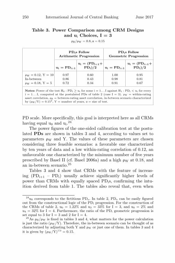
Table 3. Power Comparison among CRM Designsand ui Choices, I = 3
ρB/ρW = 0.8, α = 0.15
PDis Follow PDis FollowArithmetic Progression Geometric Progression
ui = (PDi+1+ ui = (PDi+1+ui = PDi+1 PDi)/2 ui = PDi+1 PDi)/2
ρW = 0.12, Y = 10 0.97 0.60 1.00 0.95In-between 0.86 0.43 0.98 0.81ρW = 0.18, Y = 5 0.72 0.34 0.91 0.67
Notes: Power of the test H0 : PDi ≥ ui for some i = 1. . . I against H1 : PDi < ui for everyi = 1. . . I, computed at the postulated PDs of table 2 (case I = 3). ρW = within-ratingasset correlation, ρB = between-rating asset correlation, in-between scenario characterizedby (ρW/Y) = 0.152, Y = number of years, α = size of test.
PD scale. More specifically, this goal is interpreted here as all CRMshaving equal u0 and ui.24
The power figures of the one-sided calibration test at the postu-lated PDs are shown in tables 3 and 4, according to values set toparameters ρW and Y. The values of these parameters are chosenconsidering three feasible scenarios: a favorable one characterizedby ten years of data and a low within-rating correlation of 0.12, anunfavorable one characterized by the minimum number of five yearsprescribed by Basel II (cf. Basel 2006a) and a high ρW at 0.18, andan in-between scenario.25
Tables 3 and 4 show that CRMs with the feature of increas-ing (PDi+1 – PDi) usually achieve significantly higher levels ofpower than CRMs with equally spaced PDis, confirming the intu-ition derived from table 1. The tables also reveal that, even when
24u0 corresponds to the fictitious PDo. In table 2, PDo can be easily figuredout from the constructional logic of the PDi progression. For the construction ofthe CRMs of table 2, u0 = 1.22% and u3 = 33% for I = 3, and u0 = 2% andu4 = 32% for I = 4. Furthermore, the ratio of the PDi geometric progression isset equal to 3 for I = 3 and 2 for I = 4.
25As ρB/ρW is fixed in tables 3 and 4, what matters for the power calculationis just the ratio (ρW/Y). Therefore, the in-between scenario can be thought of ascharacterized by adjusting both Y and ρW or just one of them. In tables 3 and 4it is given by (ρW/Y)1/2 = 0.15.

Vol. 13 No. 2 Joint Validation of Credit Rating PDs 251
Table 4. Power Comparison among CRM Designsand ui Choices, I = 4
ρB/ρW = 0.8, α = 0.15
PDis Follow PDis FollowArithmetic Progression Geometric Progression
ui = (PDi+1+ ui = (PDi+1+ui = PDi+1 PDi)/2 ui = PDi+1 PDi)/2
ρW = 0.12, Y = 10 0.82 0.39 0.95 0.68In-between 0.62 0.28 0.81 0.48ρW = 0.18, Y = 5 0.49 0.22 0.65 0.37
Notes: Power of the test H0 : PDi ≥ ui for some i = 1. . . I against H1 : PDi < ui for everyi = 1. . . I, computed at the postulated PDs of table 2 (case I = 4). ρW = within-ratingasset correlation, ρB = between-rating asset correlation, in-between scenario characterizedby (ρW/Y) = 0.151/2, Y = number of years, α = size of test.
solely focusing on the former, more demanding requirements for ui(cf. ui = (PDi+1+ PDi)/2) may produce overly conservative tests,with, for example, power on the level of only 37 percent. Thereforeliberal strategies for ui (cf. ui = PDi+1) seem to be necessary for real-istic validation attempts, and attention is focused on these strategiesin the remainder of this section. Further from the tables, the poweris found to be very sensitive to the within-rating correlation ρW andto the number of years Y. It can increase more than 80 percent fromthe worst to the best scenario (cf. last column of table 4).
While in previous tables the between-rating correlation param-eter ρB is held fixed, tables 5 and 6 examine its effect, along a setof feasible values, on the power of the test. Power is computed atthe postulated PDs of CRMs of table 2 with ui = PDi+1, I = 4 andfor the in-between scenario of parameters of ρW and Y. The tablesshow just a minor effect of ρB, regardless of the size of the test andthe CRM design. Therefore, narrowing down the uncertainty in thevalue of ρB value is not of great importance if just approximate levelsof power are desired at postulated PDs. The elements that indeeddrive the power of the test are unveiled in the next analysis.
Tables 7 and 8 provide insights on the relative role played bythe different ratings on the power. Power is computed at postulatedPDs for a sequence of four embedded CRMs, starting with the CRMwith equally spaced PDs of the second line of table 7 (the CRM with

252 International Journal of Central Banking June 2017
Table 5. Effect of ρB when PDis FollowArithmetic Progression
ui = PDi+1, (ρW/Y)1/2 = 0.15, I = 4
α = 5% α = 10% α = 15%
ρB/ρW = 0.6 0.32 0.47 0.58ρB/ρW = 0.7 0.35 0.50 0.60ρB/ρW = 0.8 0.38 0.52 0.62ρB/ρW = 0.9 0.41 0.55 0.65
Notes: Power of the test H0 : PDi ≥ ui for some i = 1. . . I against H1 : PDi < uifor every i = 1. . . I, computed at the postulated PDs of table 2 (case I = 4, ui =PDi+1, PDis follow arithmetic progression). ρW = within-rating asset correlation,ρB = between-rating asset correlation, Y = number of years, α = size of the test.
Table 6. Effect of ρB when PDis FollowGeometric Progression
ui = PDi+1, (ρW/Y)1/2 = 0.15, I = 4
α = 5% α = 10% α = 15%
ρB/ρW = 0.6 0.54 0.69 0.78ρB/ρW = 0.7 0.56 0.71 0.79ρB/ρW = 0.8 0.60 0.73 0.81ρB/ρW = 0.9 0.62 0.74 0.82
Notes: Power of the test H0 : PDi ≥ ui for some i = 1. . . I against H1 : PDi < uifor every i = 1. . . I, computed at the postulated PDs of table 2 (case I = 4, ui =PDi+1, PDis follow geometric progression). ρW = within-rating asset correlation,ρB = between-rating asset correlation, Y = number of years, α = size of the test.
increasing PD differences of the second line of table 8). Each nextCRM in table 7 (table 8) is built from its antecedent by droppingthe less risky (riskiest) rating. Power is computed for the in-betweenscenario and ui = PDi+1. The tables reveal that as the number ofratings diminishes, the power increases just to a minor extent, pro-vided the riskiest (less risky) ratings are always kept in the CRM.Thus it can be said that in table 7 (table 8) the highest (lowest) PDisdrive the power of the test. This is partly intuitive because the high-est (lowest) PDis correspond to the smallest differences (ui – PD i) in

Vol. 13 No. 2 Joint Validation of Credit Rating PDs 253
Table 7. Influence of Distinct PDis on PowerPDis follow arithmetic progression;
ρB/ρW = 0.6; (ρW/Y)1/2 = 0.15; ui = PDi+1
PDis α = 5% α = 10% α = 15%
2%, 9.5%, 17%, 24.5% 0.32 0.47 0.589.5%, 17%, 24.5% 0.32 0.47 0.5817%, 24.5% 0.34 0.49 0.5924.5% 0.44 0.58 0.68
Notes: Power of the test H0 : PDi ≥ ui for some i = 1. . . I against H1 : PDi < uifor every i = 1. . . I, for I = 4. . . 1, computed at the PDs of the first column. ρW =within-rating asset correlation, ρB = between-rating asset correlation, Y = numberof years, α = size of the test.
Table 8. Influence of Distinct PDis on PowerPDis follow geometric progression;
ρB/ρW = 0.6; (ρW/Y)1/2 = 0.15; ui = PDi+1
PDis α = 5% α = 10% α = 15%
2%, 4%, 8%, 16% 0.54 0.69 0.782%, 4%, 8% 0.54 0.69 0.782%, 4% 0.56 0.71 0.792% 0.65 0.77 0.84
Notes: Power of the test H0 : PDi ≥ ui for some i = 1. . . I against H1 : PDi < uifor every i = 1. . . I, for I = 4. . . 1, computed at the PDs of the first column. ρW =within-rating asset correlation, ρB = between-rating asset correlation, Y = numberof years, α = size of the test.
the CRMs of table 7 (table 8) and because distinct PDis contributeto the power differently just to the degree their differences (ui –PD i) vary.26 The surprising part of the result refers to the degree ofrelative low importance of the dropped PDis: the variation of powerbetween I = 1 and I = 4 can be merely around 10 percent. This
26It is easy to see that for the CRMs with equally spaced PDis, (ui– PDi) istrivially constant in i but the Φ−1-transformed difference (ui – PD i) decreasesin i. For the CRMs with increasing (PDi+1 – PDi,), (ui – PDi) trivially increasesin i and the Φ−1-transformed difference (ui – PD i) increases in i too.

254 International Journal of Central Banking June 2017
latter observation should be seen as a consequence of the functionalform of DRAPM, particularly the choice of the normal copula forthe (transformed) default rates and the form of Σ.27
A message embedded in the previous tables is that in some quitefeasible cases (e.g., Y = 5 years available at the database, ρW =0.18 reflecting the portfolio default volatility, α < 15% desired), theone-sided calibration test can have substantially low power (e.g.,lower than 50 percent at the postulated PD). Another related prob-lem refers to the test not being similar on the boundary betweenthe hypotheses and therefore biased (if I > 1).28 To cope with thesedeficiencies, the statistical literature contains some proposals of non-monotone uniformly more powerful tests for the same problem, suchas in Liu and Berger (1995) and McDermott and Wang (2002).The new tests are constructed by carefully enlarging the rejectionregion in order to preserve the size α. The enlargement triviallyimplies power dominance. The new tests have two main disadvan-tages though. First, from a supervisory standpoint, non-monotonerejection regions are harder to defend on an intuitive basis becausethey imply that a bank could pass from a state of validated CRMto a state of non-validated CRM if default rates for some of theratings decrease. Second, from a theoretical point of view, Perlmanand Wu (1999) note that the new tests do not dominate the orig-inal test in the decision-theoretic sense because the probability ofvalidation under H0 (i.e., when the CRM is incorrect) is also higherfor them. The authors conclude that UMP tests should not be pur-sued at any cost, particularly at the cost of intuition. This is the viewadopted in this study, so the new tests are not explored further in thispaper.
Yet, one may try to include some prior knowledge in the formula-tion of the one-sided calibration test as a strategy for power improve-ment. Notice, first, that the size α of the test is attained when all but
27Bluemke (2013) also shows situations in which the power of validation testsis driven by a single rating, but he does not address the influence of the CRMdesign in determining what this rating is.
28A test is α-similar on a set A if the probability of rejection is equal to α every-where there. A test is unbiased at level α if the probability of rejection is smallerthan α everywhere in H0 and greater than α everywhere in H1. Every unbiasedtest at level α with a continuous power function is α-similar in the boundarybetween H0 and H1 (Gourieroux and Monfort 1995).
Vol. 13 No. 2 Joint Validation of Credit Rating PDs 255
one of the PDis go to 0 while the remaining one is set fixed at ui.29
This is probably a very unrealistic scenario against which the bankor the supervisor would like to be protected. The bank/supervisormay alternatively remove by assumption this unrealistic case fromthe space of PD possibilities and rather consider that part of theinformation to be tested is true. Notably, it can be assumed that thepostulated PDi−1, not 0, represents a lower bound for PDi, for everyrating i. A natural modification of the test consists then on replacingzα with a smaller constant c > 0 to adjust to the removed unrealis-tic PD scenarios,30 with resulting enlargement of the critical regionand achievement of a more powerful test. (Recall the definition ofthe critical region in (5).) Hence, c is defined by the requirement thatthe size of the modified test (with c instead of zα) in the reducedPD space is α. Similarly to Sasabuchi (1980), the determination ofc needs the examination of only the PD vectors with all but one oftheir coordinates’ PDis equal to their lower bounds (the postulatedPDi−1s), and the remaining one, say PDj, set at uj, for j varying in1. . . I. More formally,
Max1≤j≤I(ΦI(−c + (u1 − PD0)/(ρW/Y)1/2, . . . ,−c, . . . ,
− c + (uI − PDI−1)/(ρW/Y)1/2; ρB/ρW) = α31, (9)
from which the value of c can be derived.However, produced results indicate the previous modification
approach is of limited efficacy to power improvement. More specifi-cally, computed results indicate that the power increase is relevantonly in the region of small (probably unrealistic) ratio ρB/ρW or forambitious choices of ui (i.e., close to PDi). In the latter case, theincrease is not sufficient, however, to the achievement of reasonablelevels of power because the original levels are already too low (cf.table 1, for example). Those results are consistent with the intuitionderived from the analysis of tables 7 and 8.
29Note PDi → 0 ⇒ PDi → −∞. The limiting PD vector is in H0 and, there-fore, should not be validated. It has a probability of validation equal to α.
30As the coordinates of the input to the power function cannot go to infinityas before, –c > –zα for the size to be achieved.
31PD0 is here just a lower bound to PD1. It could be −∞ or defined subjectivelybased on accumulated practical experience. Note that the new critical region willnow depend on ρB and that the calculation of c needs some computational effort.

256 International Journal of Central Banking June 2017
On the other hand, one may also try to derive the LRT based onthe restricted PD parameter space:
Ho : PDi ≥ ui for some i = 1. . . I and
PDi ≥ postulated PDi−1 for every i = 1. . . I
H1 : PDi < ui for every i = 1. . . I and
PDi ≥ postulated PDi−1 for every i = 1. . . I.32
The LRT will differ from the modification approach with respectto the information contained in the observed default rates. The LRTwill have very small observed average default rates, providing lowerrelative evidence in favor of H1 because, by assumption, they cannotbe explained by very small PDs.33 Accordingly, the null distributionof the likelihood-ratio (LR) statistic doesn’t need to put mass onthose unrealistic PD scenarios. Unfortunately, to the best of theauthor’s knowledge, the derivation of the LRT critical region forsuch a problem is lacking in the statistical literature. Its complex-ity arises from the facts that, in contrast to the original one-sidedcalibration test, H0 and H1 do not share the same boundary in �I
and that the boundary indeed shared is a limited set. Thus, it is rea-sonable to conjecture that the null distribution of the LR statisticwill be fairly complicated. And similarly to the previous strategy, ifui >> postulated PD i−1 for most ratings, the increase in power islikely to negligible again.34
4.2 Two-Sided Calibration Testing
The section now comments on two-sided calibration testing, mostlyfrom a theoretical perspective. Similarly to the one-sided version,the hypotheses of a two-sided test can be stated as follows:
32H1 need not be defined only by strict inequalities here since the union H0 UH1 does not span the full �I space.
33Very small observed average default rates in the sense that Φ−1(DRi)/(1 −ρW)1/2 < Φ−1(postulated PDi−1).
34It is important to remark that if I is large, strategies of power improvementwill generally have more chances of relative success, although they depart fromlower original levels of power.
Vol. 13 No. 2 Joint Validation of Credit Rating PDs 257
Ho : PDi ≥ ui or PD i ≤ li for some i = 1. . . I
H1 : li < PD i < ui for every i = 1. . . I.
Now the acceptable indifference region is defined by two parame-ters ui and li for each rating i, with ideally li ≥ postulated PDi−1 andui ≤ postulated PDi+1. Under that formulation, the test belongs tothe class of multivariate equivalence tests, which are tests designedto show similarity rather than difference and are widely employedin the pharmaceutical industry (under the denomination of bio-equivalent tests) to demonstrate that drugs are equivalent. Bergerand Hsu (1996) comprehensively review the recent development ofequivalence tests in the univariate case (I = 1). The standard proce-dure to test univariate equivalence is the TOST test (two one-sidedtests—called this because the procedure is equivalent to performingtwo size-α one-sided tests and concluding equivalence only if bothreject). Wang, Hwang, and Dasgupta (1999) discuss the extension ofTOST to the multivariate case, making use of the intersection-unionmethod.35 When applied to the DRAPM distribution, that extensionresults in the following critical region for the two-sided calibrationtest.36
Reject Ho (i.e., validate the CRM) if
li/(1 − ρW)1/2 + zα(ρW/(Y(1 − ρW)))1/2
≤ DRi ≤ ui/(1 − ρW)1/2 − −zα(ρW/(Y(1 − ρW)))1/2 (10)
for every i = 1 . . . I.As the maximum power of the test occurs in the middle point of
the cube [liui]I, it is reasonable to make the cube symmetric aroundthe postulated PD (in other words, to make ui – PD i = PD i − lifor every i), so that the highest probability of validating the CRMoccurs exactly at the postulated PD. Additional configurations ofthe indifference region may include, as in the one-sided test, choosingui = PD i+1 or li = PD i−1 (but not both).
35Wang, Hwang, and Dasgupta (1999) also show that TOST is basically an LRtest.
36The standard TOST is formulated assuming unknown variance, while theproposed two-sided calibration test of this paper assumes known variance. There-fore the reference to the term TOST encompasses here some freedom of notation.

258 International Journal of Central Banking June 2017
Similarly to the one-sided test, the two-sided version has prob-lems of lack of power and bias.37 In this respect, the statistical lit-erature contains some proposals for improving TOST (Berger andHsu 1996; Brown, Hwang, and Munk 1998), which are again sub-ject to criticism from an intuitive point of view by Perlman andWu (1999).38 Furthermore, an additional drawback of the two-sidedtest, in contrast to the original TOST, is its excess of conservatismbecause the test is only level α, while its size may be much smaller.39
That observation indicates the magnified difficulty in performingtwo-sided calibration testing.
Yet, two additional approaches to testing multivariate equiv-alence deserve comments. The first one is developed by Brown,Casella, and Hwang (1995). Applied to the problem of PD cali-bration testing, it consists of accepting an alternative hypothesis H1(i.e., validating the CRM) if the Brown confidence set for the PDvector is entirely contained in H1. The approach would allow thebank or the supervisor to separate the execution of the test fromthe task of defining an indifference region because H1 configurationcould be discussed at a later stage, after the knowledge of the formof the set. In particular, the confidence set can be seen as the small-est indifference region that still permits validation of the calibration.Brown, Casella, and Hwang (1995) propose an optimal confidenceset in the sense that if the true PD vector is equal to the postulatedone, then the expected volume of that set is minimal, which meansthat, in average terms, maximal precision is achieved when calibra-tion is exactly right. The cost of this optimality is larger set volumesfor PDs different from the postulated one. Munk and Pfluger (1999)show in simulation exercises that the power of Brown’s procedurecan be substantially lower than those of more standard tests, likethe TOST, for a wide range of PDs close to the postulated one.Therefore, in light of the view of this paper that ratings could more
37If I > 1, the test is not similar on the boundary between the hypotheses andis therefore biased.
38However, in the case of calibration testing with known variance, the bias isnot as pronounced as in the standard TOST with unknown variance, due to theimpossibility of making the variance go to 0 as in Berger and Hsu (1996).
39It can be shown that the degree of conservatism depends on ρB. The reasonfor the discrepancy with the standard TOST relates again to the impossibility ofmaking the variance go to 0 as in Berger and Hsu (1996).

Vol. 13 No. 2 Joint Validation of Credit Rating PDs 259
realistically be seen as PD intervals, the benefit of the optimalityat a single point is doubtful at a minimum. Consequently, Brown’sapproach is regarded here as of more theoretical than practical valueto calibration testing.40
The second different approach to testing multivariate equivalenceis developed by Munk and Pfluger (1999). So far, this paper has justconsidered rectangular sets in the H1 statements of the calibrationtests. The goal has been to show that the true PD lies in a rectan-gle or in a quadrant of the space �I. The referred authors analyzeinstead the use of ellipsoidal alternatives for the multivariate equiv-alence problem, which, for purposes of calibration testing, can beexemplified as follows:
Ho : etDe ≥ Δ
H1 : etDe < Δ,
where e = PD – postulated PD , D is a positive definite matrix,which conceives a notion of distance in �I, and Δ denotes a fixedtolerance bound. D and Δ define an indifference region for PD.
Munk and Pfluger (1999) advocate this formulation to allow thenotion of equivalence to be interpreted as a combined measure ofseveral parameters (e.g., a combination of the PDis, i = 1. . . I). As aconsequence, this implies that very good marginal equivalence (e.g.,the true PD1 is very close to the postulated PD1) should allow largerindifference regions for the other parameters (e.g., the other PDis).Conceptually, though, this point is hard to justify in the validationof CRMs unless miscalibration were necessarily derived from a sys-tematic erroneous estimation of all the PDis. Nevertheless, the viewof this paper is that miscalibration could be rather rating specific.Furthermore, note that the rectangular alternatives already permita lot of flexibility in allowing different indifference interval lengthsfor different ratings. Consequently, for purposes of calibration test-ing, ellipsoidal alternatives are regarded here more as a practicalcomplication.41
40Other confidence set approaches to calibration testing are also possible. Someof them are, however, dominated by the multivariate TOST (Munk and Pfluger1999).
41However, for purposes of power improvement, it still might be useful to inves-tigate ellipsoidal alternatives inscribed or approximating rectangular alternatives.This investigation is not addressed in this paper.
260 International Journal of Central Banking June 2017
5. Tests of Rating Discriminatory Power
One of the most traditional measures of discriminatory power isthe area under the ROC curve (AUROC).42 Let n and m be twodistinct random borrowers with probabilities of default PDn andPDm, respectively. Following Bamber (1975), AUROC is defined as
AUROC = Prob(PDn > PDm| n defaults and m doesn’t)
+ 1/2 · Prob(PDn = PDm| n defaults and m doesn’t).(11)
High values of AUROC (close to 1) are typically interpreted asevidence of good CRM discriminatory performance. However, thedefinition of AUROC as the probability of an event concerning therealizations of two (random) borrowers makes it a function not onlyof the PD vector but also of the default correlation structure.43
To the extent that the CRM should not be held accountable forthe effect of default dependency between borrowers, the AUROCmeasure of discrimination becomes distorted.44 Blochlinger (2012)shows this distortion by means of a numerical example. The propo-sition below shows formally the dependency of AUROC on the assetcorrelation parameters.
Proposition. Consider an extension of DRAPM in which (ρij) isthe matrix of asset correlations between borrowers of ratings i andj, i,j = 1. . . I. Let P(i,j) denote the probability of two random bor-rowers having ratings i and j and P(i) the probability of one randomborrower having rating i. Then
AUROC =
∑i>j Φ2 (PDi, −PDj , −ρij)P(i,j) + 1
2
∑i Φ2 (PDi, −PDi, −ρii) P(i)
∑i,j Φ2 (PDi, −PDj , −ρij) P(i,j)
(12)
42ROC = receiver operating characteristic curve (cf. Bamber 1975). 0 ≤AUROC ≤ 1.
43It is a function of the distribution of borrowers across the ratings too.44Note that, in contrast, the definition of good calibration is always purely
linked to the good quality of the PD vector, although the way to empiricallyconclude that will typically depend on the default correlation values, as shownin section 4.

Vol. 13 No. 2 Joint Validation of Credit Rating PDs 261
Proof. See appendix 2.
Blochlinger (2012) proposes a measure of discriminatory powerthat is not a function of default dependency. However, in contrastto AUROC, it is a function of the portfolio-wide true (unknown)PD and, besides, his asymptotic testing results are based on a mul-tiplicative form for the conditional PDs not obeyed by the BaselII model or DRAPM (equation (2) is not of multiplicative form).This section describes alternatives for tests of rating discrimina-tory power built upon the DRAPM distribution. The qualifyingterm rating is added purposefully to the traditional expression “dis-criminatory power” to emphasize that the property desired to beconcluded/measured here is different from that embedded in tra-ditional measures of discriminatory power. Rather than verifyingthat the ex post rating distributions of the default and non-defaultgroups of borrowers are as separate as possible, the proposed testsof rating discriminatory power aim at showing that PDi is a strictlyincreasing function of i. In other words, the discriminatory powershould be present at the rating level or, more concretely, low-qualityratings should have larger PDis. Note that this is a less stringentrequirement than correct two-sided calibration and the alternativehypothesis here will, therefore, strictly contain the H1 of the two-sided calibration test.45 In this sense, the fulfillment of good ratingdiscriminatory power is consistent with the pursuit of correct cali-bration. Furthermore, as the proposed tests are based on hypothesesinvolving solely the PD vector, they are not functions of default cor-relations; consequently, they address the two pitfalls of traditionalmeasures of discriminatory power that were discussed in the intro-duction. Finally, showing PD monotonicity along the rating dimen-sion is also useful to corroborate the assumptions of some methodsof PD inference on low default portfolios (e.g., Pluto and Tasche2005).
This section distinguishes between a test of general rating dis-criminatory power and a test of focal rating discriminatory power.The former addresses a situation where the bank or supervisor is
45Provided ui < li+1 for i = 1. . . I – 1, as expected in practical applications. Onits turn, Blochlinger (2012) investigates a less stringent requirement than correcttwo-sided calibration but a more demanding one than PD monotonicity, namelythat PD ratios between ratings equal specific constants.

262 International Journal of Central Banking June 2017
uncertain about the increasing PD behavior along the whole ratingscale, whereas the latter focuses on a pair of consecutive ratings.The formulation of the general test is proposed below.
Ho : PDi ≥ PDi+1 for some i = 1. . . I – 1
H1 : PDi < PDi+1 for every i = 1. . . I – 1.
By viewing PD i+1 – PD i as the unknown parameter to be esti-mated (up to a constant) by DRi+1 – DRi for every rating i, theprevious test involves testing strict homogeneous inequalities aboutnormal means. (The key observable variables are now default ratedifferences between consecutive ratings, rather than the default ratesthemselves, as in the one-sided calibration test.) So, similarly to theone-sided calibration test, a size-α likelihood-ratio critical region canbe derived.
Reject H0 (i.e., validate the CRM) if
DRi+1 − DRi > zα(2(ρW − ρB)/(Y(1 − ρW)))1/2
for every i = 1. . . I – 1. (13)
It is worth noting above that, differently from the calibrationtests, there is no need for the configuration of an indifference region,as the desired H1 conclusion is already defined by strict inequal-ities. On the other hand, now the critical region and—therefore,the decision itself to validate the CRM—depends on the unknownparameter ρB. The Basel II case (ρB = ρW) represents the extremeliberal situation where just an observed increasing behavior of theaverage annual default rates along the rating dimension is sufficientto validate the CRM (regardless of the confidence level α), whereasthe case ρB = 0 places the strongest requirement in the incrementalincrease of the default rate averages along the rating scale.46 In prac-tical situations, the bank or the supervisor may want to determinethe highest value of ρB such that the general test still validates theCRM and then check how this value conforms to its beliefs aboutreality.
When theoretically compared with the power of the one-sidedcalibration test, the power of the general test is notably affected by
46This is again intuitive, as low values of ρB mean that ex post informationabout one rating does not contain much information about other ratings.

Vol. 13 No. 2 Joint Validation of Credit Rating PDs 263
a trade-off of three factors.47 First, the fact that now the underlyingnormal variables are likely to have smaller variances (Var(DRi+1 –DRi) = 2(ρW − ρB)/(1− ρW) < Var(DRi) = ρW/(1− ρW), providedρB/ρW > 1/2) contributes to an increase in power. On the otherhand, the now not positive underlying correlations (Corr(DRi+1 −DRi,DRj −DRj−1) = −1/2 if i = j and 0 otherwise, compared withCorr(DRi,DRj) = ρB/ρW > 0 for i �= j) contributes to a decrease inpower.48 Finally, the presence of I – 1 statements in H1, instead of I,implies a slight increase in power too. In general, the resulting dom-inating force is to be determined by the particular choices of ρB, ρW,and I. However, computed results indicate that discrimination testpower will usually be larger than calibration power for CRM designsincluding both arithmetic and geometric progressions for the PDisand reasonable specifications for the testing parameters.49 Finally,as with calibration testing, similar comments on possible strategiesfor power improvement and their limitations apply here as well.
It is also worthwhile to discuss the situation where the bank orthe supervisor is satisfied by the “general level” of rating discrimina-tion except for a particular pair of consecutive ratings. Suppose thebank/supervisor wants to find evidence that two consecutive ratings(say ratings 1 and 2, without loss of generality) indeed distinguishthe borrowers in terms of their creditworthiness. From a supervisorystandpoint, a suspicion of regulatory arbitrage may, for instance,motivate the concern.50 To examine this issue, this section formu-lates a test of focal rating discriminatory power, whose hypothesesare stated as follows.51
47Similarly to the calibration case, the power expression can be easily derived.48Therefore, not necessarily validating rating discriminatory power is easier
than validating (one-sided) calibration.49Also, computed results in line with previous calibration findings indicate that
CRMs whose PDis follow geometric progression will generally achieve higher lev-els of power than when PDis follow arithmetic progression and their power isbasically driven by the first pairs of consecutive ratings, in the high-credit-qualitypart of the scale.
50Suspicion of regulatory arbitrage may derive from a situation where largecredit risk exposures are apparently rated with slightly better ratings so that theresulting capital charge of Basel II is diminished.
51The discussion of this section is easily generalized to the situation wheremore than one pair of consecutive ratings are to have their rating discriminatorypower verified.

264 International Journal of Central Banking June 2017
Ho : PD1 = PD2 ≤ PD3 ≤ . . . ≤ PDI
H1 : PD1 < PD2 ≤ PD3 ≤ . . . ≤ PDI .
From a mathematical point of view, the development of thelikelihood-ratio test for such a problem is more complex than themajority of the tests considered so far in this paper, because nowthe union of the null and the alternative hypotheses do not spanthe full �I, nor do the hypotheses share a common boundary. But,in contrast to the section 4 one-sided calibration LRT under PDrestriction, now both H0 and H1 are convex cones. This impliesthat the null distribution of the LR will depend on the structureof the cone C = Ho U H1, whether obtuse or acute with respect tonorm induced by
∑∑∑−1.52 In the first case, the LR statistic followsa χ2 bar distribution under H0 (Menendez, Rueda, and Salvador1992b).53 In the second case, the distribution of the LR statisticis intractable, but the test is dominated in power by a reduced testcomprised of testing just the different parts of the hypotheses Ho andH1 (Menendez and Salvador 1991; Menendez, Rueda, and Salvador1992a). It can be shown that the structure of
∑∑∑adopted in this
paper makes the cone C acute, so that the second case is the relevantone.54 The reduced dominating test takes the form below.
Ho : PD1 = PD2
H1 : PD1 < PD2.
The test above is just a particular case of the general rating dis-criminatory power test with I = 2. Accordingly, its rejection rule isgiven as follows.
52See Martın and Salvador (1988) and Menendez, Rueda, and Salvador (1992b)for the definitions of those cone types. The norm induced by
∑∑∑−1 is defined as‖x‖Σ−1 = xT Σ−1x.
53Although χ2 bar distributions are common in the theory of order-restrictedinference (Robertson, Wright, and Dykstra 1988), application of the focal testin this circumstance is not very practical, as the determination of both the LRTstatistic and the p-values are computationally intensive.
54This is true because a′iΣaj ≤ 0, i �= j, where the ai’s (ai =
(0, . . . , −1, 1, . . . , 0)’) generate the linear restrictions defining the cone C. Morespecifically, it is true that a′
iΣaj = (ρB − ρW)/(1 − ρW) if |i – j| = 1 or 0 if |i –j| ≥ 2. See the mentioned references for further details. Whether more generalbut still realistic variance structures Σ might lead to a different conclusion is aninteresting question not addressed in this paper.

Vol. 13 No. 2 Joint Validation of Credit Rating PDs 265
Reject H0 (i.e., validate the CRM) if
DR2 − DR1 > zα(2(ρW − ρB)/(Y(1 − ρW)))1/2. (14)
The dominance of the focal test by a reduced test is a surprisingresult and was long considered an anomaly of the LR principle (e.g.,Warrack and Robertson 1984). In the context of CRMs, this meansthat in order to judge the discriminatory performance of a partic-ular pair of consecutive ratings, the bank or the supervisor wouldbe in a better position if it simply disregards the prior knowledge ofthe performance of the other ratings. But how can less informationbe better? Only most recently Perlman and Wu (1999) showed thatindeed the overall picture was not so much in favor of the “dominat-ing” test, arguing that the latter presents controversial properties.For example, it rejects PDs closer to H0 than to H1.55 Nevertheless,the practitioner does not have another choice besides using the powerdominating test, because, as just observed, the null distribution ofthe LRT statistic for the focal test is unknown. Keeping that inmind, the analysis of this section provides the theoretical founda-tion to an easy-to-implement procedure that focuses solely on thesupposedly problematic pair of ratings. More interestingly, however,a generalization of the results discussed in this section suggests auniform procedure to check rating discriminatory power: select theratings whose discriminatory capacity are at stake and apply thegeneral test to them.
6. Finite-Sample Properties
All the tests discussed in this paper are based on the asymptoticdistribution of DRAPM, which assumes an infinite number of bor-rowers for each rating. This section analyzes the implications to theperformance of the one-sided calibration test of a finite but still largenumber of borrowers (N = 100 is chosen as the base case).56 Due
55Perlman and Wu (1999) conclude once again that UMP size-α tests shouldnot be pursued at any cost.
56The analysis is restricted to the one-sided calibration test not only becauseit is the main focus of this paper but also because the finite sample properties ofdiscriminatory tests are more complex to analyze when distributions of defaultrate differences are involved. Also, as perceived later in the section, the issues ofmost concern related to the finite-sample properties of the two-sided calibrationtest derive from the analysis of the one-sided case.

266 International Journal of Central Banking June 2017
to the strong reliance of the test on the asymptotic normality ofthe marginal distributions of DRAPM, it is important to verify howthe real marginals compare to the asymptotic ones. The focus on aparticular marginal allows then, for the sake of clarity, to direct theattention initially to the case I = 1. This section conducts MonteCarlo simulations of DRAPM, at the stage in which idiosyncraticrisk is not yet diversified away, for N = 100 and Y = 5, unless statedotherwise. Based on a large set of simulated average annual defaultrates and for I = 1, the effective significance level is computed as afunction of the nominal significance level α, for varying scenarios ofthe parameters true PD and ρW. In general, 200,000 simulations arerun for each scenario.
Effective confidence level = P rob
(√1 − ρW DRn − PD√
ρW /Y< −zα
),
(15)
where the probability is estimated by the empirical frequency of theevent and DRn denotes a particular simulation result.
The effective level measures the real size of the asymptotic size-αone-sided test. Alternatively, since it is expressed in the form of aprobability of rejection, the effective level can also be seen as thereal power at the postulated PD, when the asymptotic power isequal to α, of an asymptotic size-δ one-sided test, with δ < α.57
From both interpretations, the occurrence of effective levels lowerthan nominal levels means that the test is more conservative, with asmaller probability of validation in general than what is suggested bythe analysis of section 4 based on DRAPM. Effective levels higherthan nominal levels indicates the opposite: a finite-sample liberalbias.
A first general important finding derived from the performed sim-ulations for the case I = 1 is that the convergence of the lower tailsof the average (transformed) default rate distributions to their nor-mal asymptotic limits is slower and less smooth than in the case ofthe upper tails, for realistic PD values. The situation is illustratedby the pair of graphs (figure 1) calculated based on the scenarioPD = 3%, ρW = 0.20, N = 100, and Y = 5. The solid line represents
57More specifically, it is easy to see that δ = Φ(−zα − (u − PD)/(ρW/Y)1/2).

Vol. 13 No. 2 Joint Validation of Credit Rating PDs 267
Figure 1. Lower and Upper TailsPD = 3%, ρW = 0.20, N = 100, Y = 5
Notes: Solid line: Effective confidence level against the nominal size α of theasymptotic one-sided test H0 : PD ≥ u against H1 : PD < u. Dotted straightline is the identity function to ease comparison. PD = true probability of default,ρW = asset correlation, N = number of borrowers, Y = number of years.
the effective confidence level for each nominal level depicted at thex-axes, while the dotted straight line is the identity function merelydenoting the nominal level to facilitate comparison. Note that theeffective level is much farther from the nominal value in the lowertail of the distribution (depicted in the right-hand graph) than inthe upper tail (depicted in the left-hand graph). In particular, ifthe one-sided calibration test is employed at the nominal level of 10percent, the test will be much more conservative in reality, as theeffective size will be approximately only 4 percent.
Indeed, the fact that the lower tail is less well behaved isstrongly relevant to this paper’s one-sided calibration test. Underthe approach of placing the undesired conclusion in H0 (e.g., PD ≥u), rejection of the null, or equivalently validation, is obtained ifaverage default rates are small, so that the one-sided test is basedin fact on the lower tail of the distribution. On the contrary, theupper tail would be the relevant part of the distribution had theapproach of placing the “CRM correctly specified” hypothesis in H0been adopted, as in the rest of the literature. Since convergence ofthe upper tail is better behaved, the finite-sample departure from
268 International Journal of Central Banking June 2017
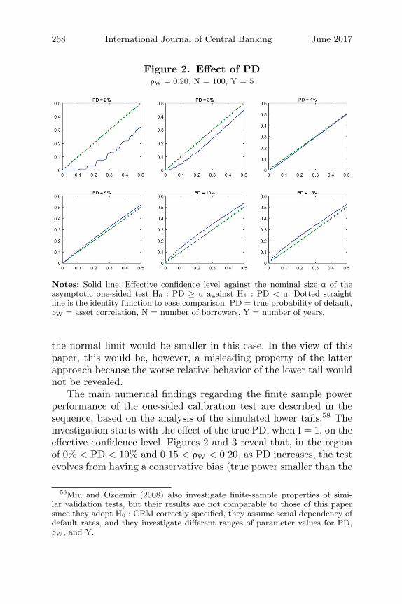
Figure 2. Effect of PDρW = 0.20, N = 100, Y = 5
Notes: Solid line: Effective confidence level against the nominal size α of theasymptotic one-sided test H0 : PD ≥ u against H1 : PD < u. Dotted straightline is the identity function to ease comparison. PD = true probability of default,ρW = asset correlation, N = number of borrowers, Y = number of years.
the normal limit would be smaller in this case. In the view of thispaper, this would be, however, a misleading property of the latterapproach because the worse relative behavior of the lower tail wouldnot be revealed.
The main numerical findings regarding the finite sample powerperformance of the one-sided calibration test are described in thesequence, based on the analysis of the simulated lower tails.58 Theinvestigation starts with the effect of the true PD, when I = 1, on theeffective confidence level. Figures 2 and 3 reveal that, in the regionof 0% < PD < 10% and 0.15 < ρW < 0.20, as PD increases, the testevolves from having a conservative bias (true power smaller than the
58Miu and Ozdemir (2008) also investigate finite-sample properties of simi-lar validation tests, but their results are not comparable to those of this papersince they adopt H0 : CRM correctly specified, they assume serial dependency ofdefault rates, and they investigate different ranges of parameter values for PD,ρW, and Y.

Vol. 13 No. 2 Joint Validation of Credit Rating PDs 269
Figure 3. Effect of PDρW = 0.15, N = 100, Y = 5
Notes: Solid line: Effective confidence level against the nominal size α of theasymptotic one-sided test H0 : PD ≥ u against H1 : PD < u. Dotted straightline is the identity function to ease comparison. PD = true probability of default,ρW = asset correlation, N = number of borrowers, Y = number of years.
asymptotic one) to having a liberal bias (true power larger than theasymptotic one). At PD = 4% for ρW = 0.20 or at PD = 3% forρW = 0.15, the finite sample bias is approximately null as the testmatches its theoretical limiting values. On the other hand, in theregion of 10% < PD < 15% and 0.15 < ρW < 0.20, as PD increases,the solid line comes back a bit closer to the dotted straight one, i.e.,the test diminishes its liberal bias (but not sufficiently so as to turnconservative).
As the asymptotic one-sided test based on DRAPM already suf-fers from problems of lack of power, this section suggests, as a pos-sible general recommendation, consideration of the real (unmodi-fied) applications of the test solely in the cases where the finite-sample analysis indicates a non-conservative bias. Indeed, if insteadan additional layer of conservatism is added to the already conser-vative asymptotic test, the resulting procedure may hardly validateat all. The restriction to the finite-sample liberal cases, when I = 1,
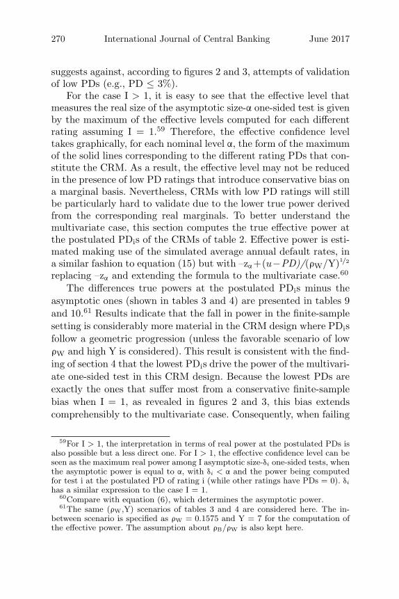
270 International Journal of Central Banking June 2017
suggests against, according to figures 2 and 3, attempts of validationof low PDs (e.g., PD ≤ 3%).
For the case I > 1, it is easy to see that the effective level thatmeasures the real size of the asymptotic size-α one-sided test is givenby the maximum of the effective levels computed for each differentrating assuming I = 1.59 Therefore, the effective confidence leveltakes graphically, for each nominal level α, the form of the maximumof the solid lines corresponding to the different rating PDs that con-stitute the CRM. As a result, the effective level may not be reducedin the presence of low PD ratings that introduce conservative bias ona marginal basis. Nevertheless, CRMs with low PD ratings will stillbe particularly hard to validate due to the lower true power derivedfrom the corresponding real marginals. To better understand themultivariate case, this section computes the true effective power atthe postulated PDis of the CRMs of table 2. Effective power is esti-mated making use of the simulated average annual default rates, ina similar fashion to equation (15) but with –zα+(u−PD)/(ρW/Y)1/2
replacing –zα and extending the formula to the multivariate case.60
The differences true powers at the postulated PDis minus theasymptotic ones (shown in tables 3 and 4) are presented in tables 9and 10.61 Results indicate that the fall in power in the finite-samplesetting is considerably more material in the CRM design where PDisfollow a geometric progression (unless the favorable scenario of lowρW and high Y is considered). This result is consistent with the find-ing of section 4 that the lowest PDis drive the power of the multivari-ate one-sided test in this CRM design. Because the lowest PDs areexactly the ones that suffer most from a conservative finite-samplebias when I = 1, as revealed in figures 2 and 3, this bias extendscomprehensibly to the multivariate case. Consequently, when failing
59For I > 1, the interpretation in terms of real power at the postulated PDs isalso possible but a less direct one. For I > 1, the effective confidence level can beseen as the maximum real power among I asymptotic size-δi one-sided tests, whenthe asymptotic power is equal to α, with δi < α and the power being computedfor test i at the postulated PD of rating i (while other ratings have PDs = 0). δi
has a similar expression to the case I = 1.60Compare with equation (6), which determines the asymptotic power.61The same (ρW,Y) scenarios of tables 3 and 4 are considered here. The in-
between scenario is specified as ρW = 0.1575 and Y = 7 for the computation ofthe effective power. The assumption about ρB/ρW is also kept here.

Vol. 13 No. 2 Joint Validation of Credit Rating PDs 271
Table 9. Difference between Effective and Asymptotic Powerfor Several CRM Designs and ui Choices, N = 100, I = 3
ρB/ρW = 0.8, α = 0.15
PDis Follow PDis FollowArithmetic Progression Geometric Progression
ui = (PDi+1+ ui = (PDi+1+ui = PDi+1 PDi)/2 ui = PDi+1 PDi)/2
ρW = 0.12, Y = 10 –0.01 –0.01 0.00 –0.03In-between –0.01 0.00 –0.05 –0.09ρW = 0.18, Y = 5 –0.01 –0.01 –0.11 –0.13
Notes: Effective and asymptotic power of the test H0 : PDi ≥ ui for some i = 1. . . Iagainst H1 : PDi < ui for every i = 1. . . I, computed at the postulated PDs of table 2(case I = 3). ρW = within-rating asset correlation, ρB = between-rating asset correlation,in-between scenario characterized by (ρW/Y) = 0.152, Y = number of years, α = asymp-totic size of test. Effective power computed based on 200,000 Monte Carlo simulations ofDRAPM.
Table 10. Difference between Effective and Asymptotic Powerfor Several CRM Designs and ui Choices, N = 100, I = 4
ρB/ρW = 0.8, α = 0.15
PDis Follow PDis FollowArithmetic Progression Geometric Progression
ui = (PDi+1+ ui = (PDi+1+ui = PDi+1 PDi)/2 ui = PDi+1 PDi)/2
ρW = 0.12, Y = 10 –0.02 –0.01 –0.03 –0.03In-between –0.02 –0.01 –0.08 –0.06ρW = 0.18, Y = 5 –0.01 –0.01 –0.11 –0.08
Notes: Effective and asymptotic power of the test H0 : PDi ≥ ui for some i = 1. . . Iagainst H1 : PDi < ui for every i = 1. . . I, computed at the postulated PDs of table 2(case I = 4). ρW = within-rating asset correlation, ρB = between-rating asset correlation,in-between scenario characterized by (ρW/Y) = 0.152, Y = number of years, α = asymp-totic size of test. Effective power computed based on 200,000 Monte Carlo simulations ofDRAPM.

272 International Journal of Central Banking June 2017
to validate CRMs with increasing PD differences because of largedefault rates of some low postulated PDis, a possible practical adviceis to apply the test only to the remainder of the postulated PDvector (e.g., ratings 3 to 7 in the example related to table 1). Alter-natively, if suspicion of PD undercalibration is particularly placed onthe low postulated PDis, a higher nominal level α could be appliedjust to them.
In the CRM design where PDis follow an arithmetic progression,the highest PDis drive the power of the test (see section 4), but theysuffer instead from a small liberal finite-sample bias. Consequently,with equally spaced PDis, the effective power of the multivariatetest is not greatly affected, as noticed in tables 9 and 10. This isparticularly useful since the asymptotic power in this CRM design isalready low compared with CRMs with increasing PD differences (asdiscussed in section 4). Tables 9 and 10 finally reveal that the choiceof the indifference region is generally of secondary importance to themagnitude of the finite-sample bias of the test in comparison withthe choice of the rating PDis, unless the favorable (ρW,Y) scenariois considered.
The influence of the within-rating asset correlation ρW under thebase case of N = 100 is analyzed in figure 4. Considering initiallythe case I = 1, one notes that when ρW increases, the test evolvestowards a more conservative bias (or towards a smaller liberal one),for every PD. Note that this represents a second channel, nowthrough the finite-sample properties, by which ρW diminishes thepower of the test. For the case I > 1, note first that the movetowards a conservative bias is greater the lower the PD in figure4. Because the lowest rating PDis tend to drive the power of the testwhen CRMs possess increasing PD differences, it is expected thatthe finite-sample power-reducing effect of ρW will be stronger in pre-cisely that type of CRM design. This is indeed the result found intables 9 and 10 when one moves in the direction from ρW = 0.12 toρW = 0.18 and PDis follow a geometric progression.62 Consequently,
62More precisely, in tables 9 and 10, Y also changes across the parameter sce-narios. However, holding Y constant and just increasing ρW produces the samesort of result.
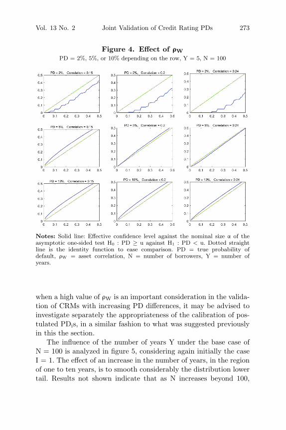
Vol. 13 No. 2 Joint Validation of Credit Rating PDs 273
Figure 4. Effect of ρWPD = 2%, 5%, or 10% depending on the row, Y = 5, N = 100
Notes: Solid line: Effective confidence level against the nominal size α of theasymptotic one-sided test H0 : PD ≥ u against H1 : PD < u. Dotted straightline is the identity function to ease comparison. PD = true probability ofdefault, ρW = asset correlation, N = number of borrowers, Y = number ofyears.
when a high value of ρW is an important consideration in the valida-tion of CRMs with increasing PD differences, it may be advised toinvestigate separately the appropriateness of the calibration of pos-tulated PDis, in a similar fashion to what was suggested previouslyin this the section.
The influence of the number of years Y under the base case ofN = 100 is analyzed in figure 5, considering again initially the caseI = 1. The effect of an increase in the number of years, in the regionof one to ten years, is to smooth considerably the distribution lowertail. Results not shown indicate that as N increases beyond 100,

274 International Journal of Central Banking June 2017
Figure 5. Effect of YPD = 5%, ρW = 0.20, N = 100
Notes: Solid line: Effective confidence level against the nominal size α of theasymptotic one-sided test H0 : PD ≥ u against H1 : PD < u. Dotted straightline is the identity function to ease comparison. PD = true probability ofdefault, ρW = asset correlation, N = number of borrowers, Y = number ofyears.
the solid and dotted lines come closer at every figure, as expected.Other produced results also indicate that, for the same Y, thelower-tail discontinuity is greater the lower the PDs. Consequently,based on the same reasoning underlying the previous analysis on theeffect of ρW, the lower-tail discontinuity propagates more stronglyto the multivariate case again when CRMs possess increasing PDdifferences.
Finally, it is important to observe that even if the one-sided testcould be totally based on the simulated distributions of this section,there would still be some extreme cases where validation is virtually

Vol. 13 No. 2 Joint Validation of Credit Rating PDs 275
impossible at traditional low confidence levels. When I = 1 andY = 1 (cf. figure 5) or true PD = 1%, for example, the lower tail ofthe distribution is quite discrete and presents significant probabil-ity of zero defaults. As a result, the effective confidence level jumpsseveral times and assumes only a small finite number of values inthe lower tail. When Y = 1 (and I = 1), the first non-zero effectivelevel is already approximately 15 percent; after that, the next valueis approximately 30 percent. Therefore, validation at the 5 percentor 10 percent significance level is not possible. Hence, the Basel IIprescription of a minimum of five years of data is important not onlyto increase the asymptotic power of the test, according to section 4,but also to remove the quite problematic finite-sample behavior ofthe lower tail.
7. Conclusion
This study contributes to the CRM validation literature by introduc-ing new ways to statistically address the validation of credit ratingPDs. Firstly, it proposes new formulations for H0 and H1 in order tocontrol the error of accepting an incorrect CRM. Secondly, it pro-vides an integrated analytical treatment of all ratings at once, in away that recognizes the effect of default correlation. Finally, it pro-vides a unified framework for testing calibration and rating discrimi-natory power. All these aspects are interlinked with the developmentof a probabilistic asymptotic normal model for the average defaultrate vector that recognizes default correlation. Important empiricaland practical consequences stem from these proposals, as outlinedin the following paragraphs.
On calibration testing, the relative roles played by the distinctelements that affect the power are unveiled for the one-sided version.The feature of increasing PD differences between consecutive rat-ings, found in many real-world CRMs, and, particularly, the choiceof liberal indifference regions are shown to be important to theachievement of reasonable levels of power. On the other hand, thecorrelation between the ratings, whose calibration is not present inBasel II, possesses only a minor effect on power. Also, appropriately

276 International Journal of Central Banking June 2017
restricting the set of PDs to be tested may do a job almost as goodas the original test in terms of power, which may offer support, inmany practical circumstances, to reduce joint validation of creditrating PDs to individual validation of a few rating PDs. Anotherimportant general message of the analysis is that the power of theone-sided calibration test is unavoidably and substantially low insome cases. Regarding this issue, strategies of power improvementare discussed, suggesting limited efficacy or inappropriateness. Addi-tionally, the paper discusses the conceptual problems of applyingmodern ideas in multivariate equivalence to two-sided calibrationtesting.
As far as discrimination is concerned, a new goal of rating dis-criminatory power is established for CRMs. In contrast to traditionalmeasures of discrimination, the new aimed property is less stringentthan the requirement of perfect calibration and is not dependenton default correlation. Results of uniform power dominance pro-vide a theoretical foundation for restricting the investigation of thedesired property just to the pairs of consecutive ratings whose dis-criminatory capacity are at stake and, therefore, lead to an easy-to-implement procedure.
Understanding the implications of DRAPM to validation alsoincludes an analysis of its properties when dealing with a finite-sample of borrowers. As a matter of fact, DRAPM has thedisadvantage of being an asymptotic model whose finite-sampleproperties may introduce a significant additional layer of test con-servatism besides the asymptotic one. Monte Carlo simulations showthat this will likely be the case for small PDs (e.g., PD ≤ 3%) or asmall number of years (e.g., Y < 5) in the one-sided calibration test.A possible recommendation in the former case may be to apply thetest just to the remaining ratings or to investigate the low postu-lated PDs at a higher nominal confidence level. On the other hand,when a liberal finite-sample bias is present, it may counterbalancethe nominal conservatism, although some caution should always beexercised in the analysis. A general more robust procedure, how-ever, would ideally try to incorporate the remaining non-systemicpart of the credit risk into the validation process. Future research iswarranted on this aspect.

Vol. 13 No. 2 Joint Validation of Credit Rating PDs 277
Above all, the bank or the regulator should not demand muchfrom statistical testing of CRMs. Even under the simplifyingassumptions of DRAPM, the power of the tests of this paper, aswell as other tests discussed in the literature, is negatively affectedby the unavoidable presence of default correlation and by the smalllength of default rate time series available in banks’ databases. Pos-sibly due to this reason, BCBS (2005b) perceives validation as com-prising not only quantitative but also somewhat qualitative tools.It is likely, for example, that the investigation of the continuousinternal use of PDs/ratings by the bank may uncover further evi-dence, although subjective, supporting or not supporting the CRMvalidation. Nonetheless, this paper supports the view that the possi-bility of reliance on qualitative aspects opened by the Basel Commit-tee should not dampen the incentives to extract as much quantitativefeedback as possible from statistical testing, including a quantitativesense of its limitations.
Appendix 1
Figure 6 should be interpreted as a result over the long run anddisplays a rating model with perfect discrimination but not per-fect calibration. The bars’ heights represent the magnitude of theex post default rate for each rating. All borrowers classified as Cto E defaulted, whereas all borrowers classified as A to B survived.If this is the regular behavior of this CRM, knowing beforehandthe rating of the obligor allows one to predict default or no defaultwith certainty (perfect discriminatory power). The thin steppedline indicates the ex ante PD estimate for each rating. Ratings Aand B had a 0 percent default rate, thus lower than the ex anteprediction. Ratings C to E had a 100 percent default rate, thushigher than the ex ante prediction. The CRM is therefore not cor-rectly calibrated. Obviously, this example represents an extreme case(because realistic CRMs do not have perfect discriminatory power),but it is useful to illustrate that although both characteristics aredesirable, they may well be inconsistent as they are aimed at theirbest.

278 International Journal of Central Banking June 2017
Figure 6. Perfect Discrimination but ImperfectCalibration
A B C D E
100%
0%
Default rate
Rating
PD estimate
Notes: The bold bar height of each rating represents the ex post long-run defaultrate of that rating, whereas the thin stepped line represents the ex ante PDestimates of the ratings.
Appendix 2
Proof of Proposition
The first parcel of the AUROC definition can be expressed as follows.
Prob(PDn > PDm|n defaults and m doesn’t)
=Prob(n defaults and m doesn’t, PDn > PDm)
Prob(n defaults and m doesn’t)
=
∑Ii,j=1 Prob(n defaults and m doesn’t, PDn > PDm|
n has rating i and m has rating j)P(i,j)∑Ii,j=1 Prob(n defaults and m doesn’t|
n has rating i and m has rating j)P(i,j)
=
∑Ii,j=1, i>j Prob(n defaults and m doesn’t |n has rating i and m has rating j)P(i,j)∑I
i,j=1 Prob(n defaults and m doesn’t|n has rating i and m has rating j)P(i,j)
=
∑Ii,j=1, i>j Φ2
(Φ−1 (PDi) , −Φ−1 (PDj) , −ρij
)P(i,j)
∑Ii,j=1 Φ2
(Φ−1 (PDi) , −Φ−1 (PDj) , −ρij
)P(i,j)
.

Vol. 13 No. 2 Joint Validation of Credit Rating PDs 279
where the last equality derives from the expression for a joint prob-ability of default and non-default implicit in a DRAPM-style model(e.g., Gordy 2000). Similarly, the second parcel of the AUROC def-inition can be expressed as
1/2 Prob(PDn = PDm|n defaults and m doesn’t)
=
I∑i=1
Φ2(Φ−1 (PDi) , −Φ−1 (PDi) , −ρii
)P(i)
2I∑
i,j=1Φ2 (Φ−1 (PDi) , −Φ−1 (PDj) , −ρij) P(i,j)
.
and the proposition is proved, observing the convention PDi ≡Φ−1(PDi).
References
Balthazar, L. 2004. “PD Estimates for Basel II.” Risk (April): 84–85.Bamber, D. 1975. “The Area Above the Ordinal Dominance Graph
and the Area Below the Receiver Operating CharacteristicGraph.” Journal of Mathematical Psychology 12 (4): 387–415.
Basel Committee on Banking Supervision. 2005a. “An ExplanatoryNote on the Basel II IRB Risk Weight Functions.” Bank forInternational Settlements.
———. 2005b. “Studies on the Validation of Internal Rating Sys-tems.” Bank for International Settlements.
———. 2006a. “Basel II: International Convergence of Capital Meas-urement and Capital Standards: A Revised Framework — Com-prehensive Version.” Bank for International Settlements.
———. 2006b. “The IRB Use Test: Background and Implementa-tion.” Bank for International Settlements.
———. 2011. “Basel III: A Global Regulatory Framework for MoreResilient Banks and Banking Systems — Revised Version.” Bankfor International Settlements.
Berger, R. L. 1989. “Uniformly More Powerful Tests for HypothesesConcerning Linear Inequalities and Normal Means.” Journal ofthe American Statistical Association 84 (405): 192–99.
Berger, R. L., and J. C. Hsu. 1996. “Bioequivalence Trials,Intersection-Union Tests and Equivalence Confidence Sets.” Sta-tistical Science 11 (4): 283–319.

280 International Journal of Central Banking June 2017
Black, F., and M. Scholes. 1973. “The Pricing of Options and Cor-porate Liabilities.” Journal of Political Economy 81 (3): 637–54.
Blochlinger, A. 2012. “Validation of Default Probabilities.” Journalof Financial and Quantitative Analysis 47 (5): 1089–1123.
Blochlinger, A., and M. Leippold. 2006. “Economic Benefit of Pow-erful Credit Scoring.” Journal of Banking and Finance 30 (3):851–73.
Blochwitz, S., S. Hohl, D. Tasche, and C. When. 2004. “ValidatingDefault Probabilities on Short Time Series.” Working Paper.
Bluemke, O. 2013. “Probability of Default Validation: Introducingthe Likelihood-Ratio Test and Power Considerations.” Journalof Risk Model Validation 7 (2): 29–59.
Brown, L. D., G. Casella, and G. Hwang. 1995. “Optimal ConfidenceSets, Bioequivalence and the Limacon of Pascal.” Journal of theAmerican Statistical Association 90 (431): 880–89.
Brown, L. D., G. Hwang, and A. Munk. 1998. “An Unbiased Testfor the Bioequivalence Problem.” Annals of Statistics 25 (6):2345–67.
Demey, P., J. F. Jouanin, C. Roget, and T. Roncalli. 2004.“Maximum Likelihood Estimate of Default Correlations.” Risk(November): 104–8.
Engelmann, B., E. Hayden, and D. Tasche. 2003. “Testing RatingAccuracy.” Risk (January).
Gordy, M. B. 2000. “A Comparative Anatomy of Credit Risk Mod-els.” Journal of Banking and Finance 24 (1–2): 119–49.
———. 2003. “A Risk-Factor Model Foundation for Ratings-BasedBank Capital Rules.” Journal of Financial Intermediation 12 (3):199–232.
Gourieroux, C., and A. Monfort. 1995. Statistics and EconometricModels, Vol. 2 (Themes in Modern Econometrics). CambridgeUniversity Press.
Hochberg, Y., and A. C. Tamhane. 1987. Multiple Comparison Pro-cedures. John Wiley & Sons, Inc.
Laska, E. M., and M. J. Meisner. 1989. “Testing Whether an Iden-tified Treatment Is Best.” Biometrics 45 (4): 1139–51.
Leland, H. E. 2004. “Predictions of Default Probabilities in Struc-tural Models of Debt.” Journal of Investment Management 2 (2):5–20.

Vol. 13 No. 2 Joint Validation of Credit Rating PDs 281
Liu, H., and R. L. Berger. 1995. “Uniformly More Powerful, One-Sided Tests for Hypotheses about Linear Inequalities.” Annalsof Statistics 23 (1): 55–72.
Martın, M., and B. Salvador. 1988. “Validity of the ‘Pool-Adjacent-Violator’ Algorithm.” Statistics and Probability Letters 6 (3):143–45.
McDermott, M. P., and Y. Wang. 2002. “Construction of UniformlyMore Powerful Tests for Hypotheses about Linear Inequalities.”Journal of Statistical Planning and Inference 107 (1–2): 207–17.
Menendez, J. A., C. Rueda, and B. Salvador. 1992a. “Dominanceof Likelihood Ratio Tests under Cone Constraints.” Annals ofStatistics 20 (4): 2087–99.
———. 1992b. “Testing Non-Oblique Hypotheses.” Communica-tions in Statistics — Theory and Method 21 (2): 471–84.
Menendez, J. A., and B. Salvador. 1991. “Anomalies of the Likeli-hood Ratio Test for Testing Restricted Hypotheses.” Annals ofStatistics 19 (2): 889–98.
Merton, R. C. 1974. “On the Pricing of Corporate Debt: The RiskStructure of Interest Rates.” Journal of Finance 29 (2): 449–70.
Miu, P., and B. Ozdemir. 2008. “Estimating and Validating Long-Run Probability of Default with Respect to Basel II Require-ments.” Journal of Risk Model Validation 2 (2): 3–41.
Munk, A., and R. Pfluger. 1999. “1-α Equivariant Confidence Rulesfor Convex Alternatives are α/2-Level Tests — With Applica-tions to the Multivariate Assessment of Bioequivalence.” Journalof the American Statistical Association 94 (448): 1311–19.
Perlman, M. D., and L. Wu. 1999. “The Emperor’s New Tests.”Statistical Science 14 (4): 355–69.
Pluto, K., and D. Tasche. 2005. “Thinking Positively.” Risk(August): 72–78.
Robertson, T., F. T. Wright, and R. L. Dykstra. 1988. OrderRestricted Statistical Inference. John Wiley & Sons.
Sasabuchi, S. 1980. “A Test of a Multivariate Normal Mean withComposite Hypotheses Determined by Linear Inequalities.” Bio-metrika 67 (2): 429–39.
Shapiro, A. 1988. “Towards a Unified Theory of Inequality Con-strained Testing in Multivariate Analysis.” International Statis-tical Review 56 (1): 49–62.
Vasicek, O. 2002. “Loan Portfolio Value.” Risk (December).

282 International Journal of Central Banking June 2017
Wang, W., J. T. G. Hwang, and A. Dasgupta. 1999. “Statistical Testsfor Multivariate Bioequivalence.” Biometrika 86 (2): 395–402.
Warrack, G., and T. Robertson. 1984. “A Likelihood Ratio TestRegarding Two Nested but Oblique Order-Restricted Hypothe-ses.” Journal of the American Statistical Association 79 (388):881–86.
Watt, M. 2013. “Mending the RWA Machine.” Risk 26 (1, January):17–20.