sensors

Article

Joint Estimation of Source Range and Depth Using aBottom-Deployed Vertical Line Array in Deep Water

Hui Li 1,2, Kunde Yang 1,2,*, Rui Duan 1,2 and Zhixiong Lei 1,2

1 School of Marine Science and Technology, Northwestern Polytechnical University, Xi’an 710072, China;ddstc2008@163.com (H.L.); duanrui@nwpu.edu.cn (R.D.); leizhixiong@163.com (Z.L.)

2 Key Laboratory of Ocean Acoustics and Sensing (Northwestern Polytechnical University),Ministry of Industry and Information Technology, Xi’an 710072, China

* Correspondence: ykdzym@nwpu.edu.cn; Tel.: +86-029-8846-0586

Academic Editors: Xiaoning Jiang and Chao ZhangReceived: 22 March 2017; Accepted: 5 June 2017; Published: 7 June 2017

Abstract: This paper presents a joint estimation method of source range and depth using abottom-deployed vertical line array (VLA). The method utilizes the information on the arrivalangle of direct (D) path in space domain and the interference characteristic of D and surface-reflected(SR) paths in frequency domain. The former is related to a ray tracing technique to backpropagate therays and produces an ambiguity surface of source range. The latter utilizes Lloyd’s mirror principleto obtain an ambiguity surface of source depth. The acoustic transmission duct is the well-knownreliable acoustic path (RAP). The ambiguity surface of the combined estimation is a dimensionless adhoc function. Numerical efficiency and experimental verification show that the proposed method is agood candidate for initial coarse estimation of source position.

Keywords: joint localization; vertical line array; reliable acoustic path

1. Introduction

The features of reliable acoustic path (RAP) as a stable acoustic transmission duct in the deep oceanhave been studied extensively [1–3]. The definition of RAP requires a positive critical depth, whichspecifies that the ocean environment supports long-range propagation without bottom interaction.However, in practice, when the positive critical depth does not exist but the ocean is sufficiently deep,the near-bottom hydrophone can also receive the strong direct (D) signals from the moderate sourcerange. In addition, the interference signals from the long-distance source can also be weakened due tothe multireflection with the ocean interface. Generally, such acoustic transmission duct is also calledgeneralized RAP. The present study is under the generalized RAP environment.

Under RAP environment conditions, our previous work proposed two single-hydrophonelocalization methods for a moving radial source [4,5] and a two-hydrophone localization methodwith cross-correlation function matching [6]. Nevertheless, these methods commonly require that thesignal-to-noise ratio (SNR) is higher than 0 dB. McCargar et al. [7] introduced a source depth estimationmethod with a vertical line array (VLA) by exploiting the coherent addition structure of the D andsurface-reflected (SR) arrivals; Kniffin et al. investigated the performance metrics of this method [8].The method also requires long duration for observation, and it is vulnerable to ocean fluctuation.All these methods are associated with the multipath arrival structure at the receiver hydrophone orarray. Specifically, research only focused on the D and SR arrivals because the bottom-reflected (BR)arrivals are often not available due to the weak arrival amplitude and considerable spread in time.Other relevant studies related with source localization by employing the information of multipatharrival structure are reported in Refs. [9–12] and references therein.

Sensors 2017, 17, 1315; doi:10.3390/s17061315 www.mdpi.com/journal/sensors

Sensors 2017, 17, 1315 2 of 12

The previous methods commonly do not work well for passive detection in actual oceanenvironments due to the lack of available stable information. In practice, the VLA is a commonreceiving geometry, and it can sufficiently sample the acoustic field information for source localization.For example, matched filed processing (MFP) is a typical generalized beamforming method that usesspatial complexities of acoustic fields to localize source [13]. Generally, the signals received by a VLAinclude three kinds of source information: direction of arrival (DOA) in space domain, time delay intime domain, and interference characteristic in frequency domain. Any of them cannot accuratelylocalize the source alone. According to the ray propagation point of view, the ray paths under RAPenvironment are clear and stable. The distinct property of RAP provides very reliable information forsource localization. On the basis of the space-frequency features of RAP, we propose a joint sourcelocalization method in this paper. We utilize the spatial information in the form of arrival angle ofthe D path and the frequency-dependent interference characteristic between the D and SR paths; theformer is based on a ray backpropagation procedure, and the latter is related to Lloyd-mirror effect [14].The advantages of the proposed method include the sufficient utilization of the array aperture toestimate the DOA of the D path and the high output SNR after beamforming, which enhances theinterference characteristics in frequency domain. Finally, a dimensionless range/depth ambiguitysurface is provided. The localization results are robust. Moreover, the beamforming technique canalso potentially suppress the interference source outside the main lobe in complex environments.In Section 2, a detailed description of the method and the simulation results are given. In Section 3, theproposed method is verified using experimental data. Localization errors are discussed in Section 4.Section 5 summarizes this paper.

2. Theory and Simulation

The source localization method consists of three steps. The first step uses the VLA to estimatethe DOA of the source signal using conventional beamforming (CBF). Figure 1a shows the soundspeed profile (SSP) used in numerical simulation, this profile was obtained from an experimentalmeasurement that will be introduced in Section 3. The rays emitting from a source at 4188 m arepresented in Figure 1b. The ray bending effect obeys Snell’s law. When the arrival angle of the Dpath is obtained by CBF, the stable ray model is used to trace the possible source locations and obtaina range ambiguity surface. The second step utilizes the interference characteristic of beamformingoutput. The geometry of Lloyd’s mirror effect is illustrated in Figure 1c.

Sensors 2017, 17, 1315 2 of 11

The previous methods commonly do not work well for passive detection in actual ocean environments due to the lack of available stable information. In practice, the VLA is a common receiving geometry, and it can sufficiently sample the acoustic field information for source localization. For example, matched filed processing (MFP) is a typical generalized beamforming method that uses spatial complexities of acoustic fields to localize source [13]. Generally, the signals received by a VLA include three kinds of source information: direction of arrival (DOA) in space domain, time delay in time domain, and interference characteristic in frequency domain. Any of them cannot accurately localize the source alone. According to the ray propagation point of view, the ray paths under RAP environment are clear and stable. The distinct property of RAP provides very reliable information for source localization. On the basis of the space-frequency features of RAP, we propose a joint source localization method in this paper. We utilize the spatial information in the form of arrival angle of the D path and the frequency-dependent interference characteristic between the D and SR paths; the former is based on a ray backpropagation procedure, and the latter is related to Lloyd-mirror effect [14]. The advantages of the proposed method include the sufficient utilization of the array aperture to estimate the DOA of the D path and the high output SNR after beamforming, which enhances the interference characteristics in frequency domain. Finally, a dimensionless range/depth ambiguity surface is provided. The localization results are robust. Moreover, the beamforming technique can also potentially suppress the interference source outside the main lobe in complex environments. In Section 2, a detailed description of the method and the simulation results are given. In Section 3, the proposed method is verified using experimental data. Localization errors are discussed in Section 4. Section 5 summarizes this paper.

2. Theory and Simulation

The source localization method consists of three steps. The first step uses the VLA to estimate the DOA of the source signal using conventional beamforming (CBF). Figure 1a shows the sound speed profile (SSP) used in numerical simulation, this profile was obtained from an experimental measurement that will be introduced in Section 3. The rays emitting from a source at 4188 m are presented in Figure 1b. The ray bending effect obeys Snell’s law. When the arrival angle of the D path is obtained by CBF, the stable ray model is used to trace the possible source locations and obtain a range ambiguity surface. The second step utilizes the interference characteristic of beamforming output. The geometry of Lloyd’s mirror effect is illustrated in Figure 1c.

Figure 1. (a) Sound speed profile from an experimental measurement. (b) Ray propagation with source depth of 4188 m. (c) Geometry for Lloyd’s mirror effect.

The beamforming output contains the information about D and SR arrivals, the interference oscillation of which along frequency is used to obtain a depth ambiguity surface. The last step

Figure 1. (a) Sound speed profile from an experimental measurement. (b) Ray propagation with sourcedepth of 4188 m. (c) Geometry for Lloyd’s mirror effect.

Sensors 2017, 17, 1315 3 of 12

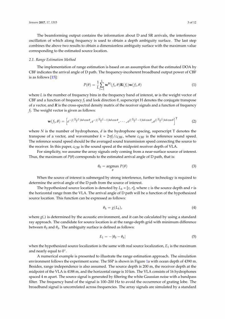
The beamforming output contains the information about D and SR arrivals, the interferenceoscillation of which along frequency is used to obtain a depth ambiguity surface. The last stepcombines the above two results to obtain a dimensionless ambiguity surface with the maximum valuecorresponding to the estimated source location.

2.1. Range Estimation Method

The implementation of range estimation is based on an assumption that the estimated DOA byCBF indicates the arrival angle of D path. The frequency-incoherent broadband output power of CBFis as follows [15]:

P(θ) =1L

L

∑l=1

wH( fl , θ)R( fl)w( fl , θ) (1)

where L is the number of frequency bins in the frequency band of interest, w is the weight vector ofCBF and a function of frequency fl and look direction θ, superscript H denotes the conjugate transposeof a vector, and R is the cross-spectral density matrix of the receiver signals and a function of frequencyfl. The weight vector is given as follows:

w( fl , θ) =[e−j( N−1

2 )kd cos θ , e−j( N−12 −1)kd cos θ , · · · , ej( N−1

2 −1)kd cos θ , ej( N−12 )kd cos θ

]T(2)

where N is the number of hydrophones, d is the hydrophone spacing, superscript T denotes thetranspose of a vector, and wavenumber k = 2πfl/cCBF, where cCBF is the reference sound speed.The reference sound speed should be the averaged sound transmission speed connecting the source tothe receiver. In this paper, cCBF is the sound speed at the midpoint receiver depth of VLA.

For simplicity, we assume the array signals only coming from a near-surface source of interest.Thus, the maximum of P(θ) corresponds to the estimated arrival angle of D path, that is:

θ0 = argmaxθ

P(θ) (3)

When the source of interest is submerged by strong interference, further technology is required todetermine the arrival angle of the D path from the source of interest.

The hypothesized source location is denoted by Lh = [z, r], where z is the source depth and r isthe horizontal range from the VLA. The arrival angle of D path will be a function of the hypothesizedsource location. This function can be expressed as follows:

θh = g(Lh), (4)

where g(.) is determined by the acoustic environment, and it can be calculated by using a standardray approach. The candidate for source location is at the range-depth grid with minimum differencebetween θ0 and θh. The ambiguity surface is defined as follows:

E1 = −|θ0 − θh| (5)

when the hypothesized source localization is the same with real source localization, E1 is the maximumand nearly equal to 0◦.

A numerical example is presented to illustrate the range estimation approach. The simulationenvironment follows the experiment scene. The SSP is shown in Figure 1a with ocean depth of 4390 m.Besides, range independence is also assumed. The source depth is 200 m, the receiver depth at themidpoint of the VLA is 4188 m, and the horizontal range is 10 km. The VLA consists of 16 hydrophonesspaced 4 m apart. The source signal is generated by filtering the white Gaussian noise with a bandpassfilter. The frequency band of the signal is 100–200 Hz to avoid the occurrence of grating lobe. Thebroadband signal is uncorrelated across frequencies. The array signals are simulated by a standard

Sensors 2017, 17, 1315 4 of 12

ray approach [16]. Figure 2a shows the normalized output power of CBF, whose peaks indicate themultipath arrival angles. The maximum power occurs at 68.8◦, which corresponds to the arrival angleof D path. The D and SR arrivals cannot be resolved on the basis that the difference of D and SR arrivalangles is too small to distinguish for CBF. The second peak at 113.7◦ is due to the arrivals relatedwith BR, whose intensity is affected by bottom parameters. Although CBF is not an optimal choice indistinguishing all the multipath arrivals, the range estimation error induced by the angle estimationerror (measurement error) is tolerated in our current study. Moreover, CBF exhibits a wide main lobethat allows the simultaneous beamforming output of D and SR paths, which is also necessary for thedepth estimation in the next subsection.

Sensors 2017, 17, 1315 4 of 11

arrivals related with BR, whose intensity is affected by bottom parameters. Although CBF is not an optimal choice in distinguishing all the multipath arrivals, the range estimation error induced by the angle estimation error (measurement error) is tolerated in our current study. Moreover, CBF exhibits a wide main lobe that allows the simultaneous beamforming output of D and SR paths, which is also necessary for the depth estimation in the next subsection.

Figure 2. (a) Norlimalized output power of CBF for the source at 200 m depth and 10 km range. (b) Ambiguity surface for range estimation with θ0 = 68.8°.

The ambiguity surface using Equation (5) is shown in Figure 2b, where the real source location is denoted by a white asterisk. The unit of the ambiguity surface is degree. The ambiguity surface presents sloping straight striation across the real source location. The average arrival angle of D and SR paths is weakly dependent on source depth [17]. Thus, Equation (5) can only provide a preliminary estimation of source range, but it fails to estimate the source depth.

2.2 Depth Estimation Scheme

The received array signal is assumed as x(t). When the estimation of arrival angle θ0 is completed, the time series y(t) is subsequently obtained after broadband CBF steering at θ0. According to image theory, the complex acoustic pressure g(f), the Fourier transform of y(t), are oscillating with frequency, and the oscillatory period is associated with the source location. The amplitude variation of g(f) takes the following simple form [14]:

2 2sin sins

fg f zR c

, (6)

where 2 2rR z r , c is the sound speed for the ideal constant SSP, zs is the source depth, and

arctan /rz r . The sinusoidal structure in Equation (6) results from the constructive or destructive addition of D and SR arrivals, whose periodicity is strongly related with the source depth and source range. The sinusoidal modulation exhibits periods of π, which yields the following:

2 sinsczf

, (7)

where Δf is the width of the modulation between nulls. The interference pattern can be transformed into source depth information by the Fourier transform scheme [18,19]. The process involves the following steps: (a) obtaining of the time series y(t) by CBF, (b) Fourier transforming y(t) to frequency domain g(f), and (c) Fourier transforming g(f) to the depth and range domain:

CBF

,sfft fftt y t g f h z r x (8)

According to Equation (8), the final step involves two variables, namely, c and φ. c is the sound speed at the receiver depth zr, and φ relies on the search range r. For different r values, Δf indicates

Figure 2. (a) Norlimalized output power of CBF for the source at 200 m depth and 10 km range.(b) Ambiguity surface for range estimation with θ0 = 68.8◦.

The ambiguity surface using Equation (5) is shown in Figure 2b, where the real source locationis denoted by a white asterisk. The unit of the ambiguity surface is degree. The ambiguity surfacepresents sloping straight striation across the real source location. The average arrival angle of D andSR paths is weakly dependent on source depth [17]. Thus, Equation (5) can only provide a preliminaryestimation of source range, but it fails to estimate the source depth.

2.2. Depth Estimation Scheme

The received array signal is assumed as x(t). When the estimation of arrival angle θ0 is completed,the time series y(t) is subsequently obtained after broadband CBF steering at θ0. According to imagetheory, the complex acoustic pressure g(f ), the Fourier transform of y(t), are oscillating with frequency,and the oscillatory period is associated with the source location. The amplitude variation of g(f ) takesthe following simple form [14]:

|g( f )| = 2R

∣∣∣∣sin(

2π fc

zs sin ϕ

)∣∣∣∣, (6)

where R =√

zr2 + r2, c is the sound speed for the ideal constant SSP, zs is the source depth, andϕ = arctan(zr/r). The sinusoidal structure in Equation (6) results from the constructive or destructiveaddition of D and SR arrivals, whose periodicity is strongly related with the source depth and sourcerange. The sinusoidal modulation exhibits periods of π, which yields the following:

zs =c

2∆ f sin ϕ, (7)

where ∆f is the width of the modulation between nulls. The interference pattern can be transformedinto source depth information by the Fourier transform scheme [18,19]. The process involves the

Sensors 2017, 17, 1315 5 of 12

following steps: (a) obtaining of the time series y(t) by CBF, (b) Fourier transforming y(t) to frequencydomain g(f ), and (c) Fourier transforming g(f ) to the depth and range domain:

x(t) →CBF

y(t) →f f t

g( f ) →f f t

h(zs, r) (8)

According to Equation (8), the final step involves two variables, namely, c and ϕ. c is the soundspeed at the receiver depth zr, and ϕ relies on the search range r. For different r values, ∆f indicatesdifferent source depth zs. Hence, the ambiguity surface h(zs,r) will be a function of search range andsearch depth.

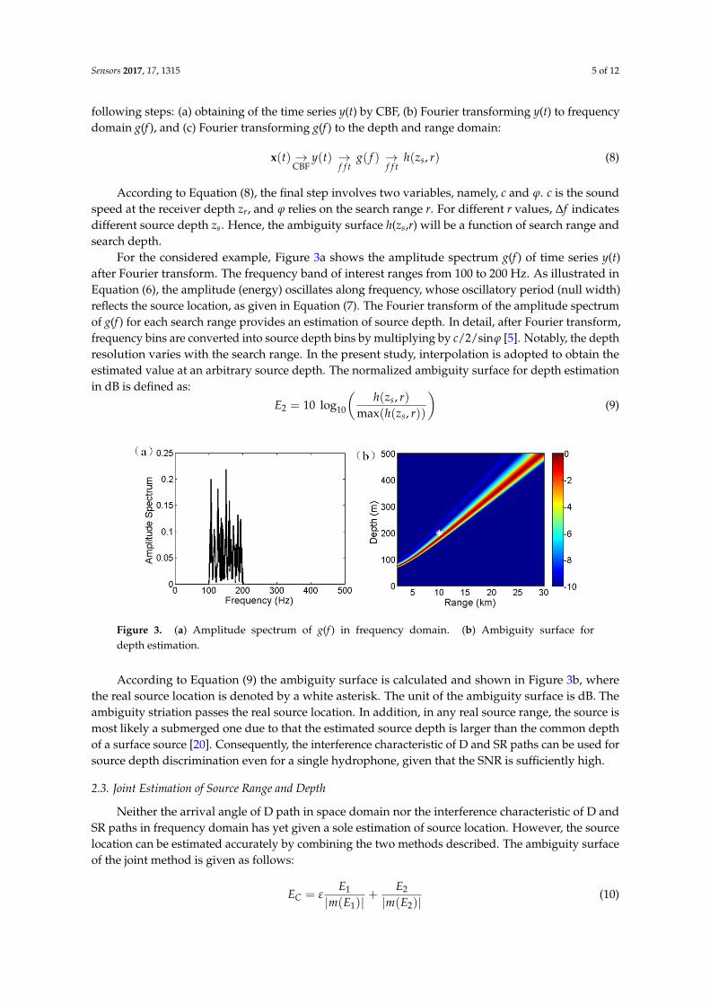
For the considered example, Figure 3a shows the amplitude spectrum g(f ) of time series y(t)after Fourier transform. The frequency band of interest ranges from 100 to 200 Hz. As illustrated inEquation (6), the amplitude (energy) oscillates along frequency, whose oscillatory period (null width)reflects the source location, as given in Equation (7). The Fourier transform of the amplitude spectrumof g(f ) for each search range provides an estimation of source depth. In detail, after Fourier transform,frequency bins are converted into source depth bins by multiplying by c/2/sinϕ [5]. Notably, the depthresolution varies with the search range. In the present study, interpolation is adopted to obtain theestimated value at an arbitrary source depth. The normalized ambiguity surface for depth estimationin dB is defined as:

E2 = 10 log10

(h(zs, r)

max(h(zs, r))

)(9)

Sensors 2017, 17, 1315 5 of 11

different source depth zs. Hence, the ambiguity surface h(zs,r) will be a function of search range and search depth.

Figure 3. (a) Amplitude spectrum of g(f) in frequency domain. (b) Ambiguity surface for depth estimation.

For the considered example, Figure 3a shows the amplitude spectrum g(f) of time series y(t) after Fourier transform. The frequency band of interest ranges from 100 to 200 Hz. As illustrated in Equation (6), the amplitude (energy) oscillates along frequency, whose oscillatory period (null width) reflects the source location, as given in Equation (7). The Fourier transform of the amplitude spectrum of g(f) for each search range provides an estimation of source depth. In detail, after Fourier transform, frequency bins are converted into source depth bins by multiplying by c/2/sinφ [5]. Notably, the depth resolution varies with the search range. In the present study, interpolation is adopted to obtain the estimated value at an arbitrary source depth. The normalized ambiguity surface for depth estimation in dB is defined as:

2 10

,10log

max( , )s

s

h z rE

h z r

(9)

According to Equation (9) the ambiguity surface is calculated and shown in Figure 3b, where the real source location is denoted by a white asterisk. The unit of the ambiguity surface is dB. The ambiguity striation passes the real source location. In addition, in any real source range, the source is most likely a submerged one due to that the estimated source depth is larger than the common depth of a surface source [20]. Consequently, the interference characteristic of D and SR paths can be used for source depth discrimination even for a single hydrophone, given that the SNR is sufficiently high.

2.3 Joint Estimation of Source Range and Depth

Neither the arrival angle of D path in space domain nor the interference characteristic of D and SR paths in frequency domain has yet given a sole estimation of source location. However, the source location can be estimated accurately by combining the two methods described. The ambiguity surface of the joint method is given as follows:

1 2

1 2

CE EE

m E m E (10)

where 1m E and 2m E are the absolute values of the averages of E1 and E2, respectively, and ε is

an adjusting factor to balance the dynamic range of E1 and E2. In this paper, ε is given as follows:

2

1

min

min

EE

(11)

Figure 3. (a) Amplitude spectrum of g(f ) in frequency domain. (b) Ambiguity surface fordepth estimation.

According to Equation (9) the ambiguity surface is calculated and shown in Figure 3b, wherethe real source location is denoted by a white asterisk. The unit of the ambiguity surface is dB. Theambiguity striation passes the real source location. In addition, in any real source range, the source ismost likely a submerged one due to that the estimated source depth is larger than the common depthof a surface source [20]. Consequently, the interference characteristic of D and SR paths can be used forsource depth discrimination even for a single hydrophone, given that the SNR is sufficiently high.

2.3. Joint Estimation of Source Range and Depth

Neither the arrival angle of D path in space domain nor the interference characteristic of D andSR paths in frequency domain has yet given a sole estimation of source location. However, the sourcelocation can be estimated accurately by combining the two methods described. The ambiguity surfaceof the joint method is given as follows:

EC = εE1

|m(E1)|+

E2

|m(E2)|(10)

Sensors 2017, 17, 1315 6 of 12

where |m(E1)| and |m(E2)| are the absolute values of the averages of E1 and E2, respectively, and ε isan adjusting factor to balance the dynamic range of E1 and E2. In this paper, ε is given as follows:

ε =

∣∣∣∣min(E2)

min(E1)

∣∣∣∣ (11)

The existence of ε will not cause any variation to the estimation results, but will provide a gooddemonstration. Equation (10) is an ad hoc cost function, and EC is dimensionless. The maximum in theambiguity surface indicates the estimated source location.

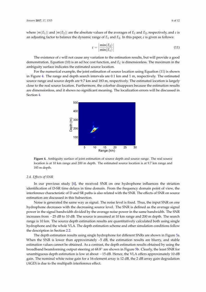
For the numerical example, the joint estimation of source location using Equation (11) is shownin Figure 4. The range and depth search intervals are 0.1 km and 1 m, respectively. The estimatedsource range and source depth are 9.7 km and 183 m, respectively. The estimated location is largelyclose to the real source location. Furthermore, the colorbar disappears because the estimation resultsare dimensionless, and it shows no significant meaning. The localization errors will be discussed inSection 4.

Sensors 2017, 17, 1315 6 of 11

The existence of ε will not cause any variation to the estimation results, but will provide a good demonstration. Equation (10) is an ad hoc cost function, and EC is dimensionless. The maximum in the ambiguity surface indicates the estimated source location.

For the numerical example, the joint estimation of source location using Equation (11) is shown in Figure 4. The range and depth search intervals are 0.1 km and 1 m, respectively. The estimated source range and source depth are 9.7 km and 183 m, respectively. The estimated location is largely close to the real source location. Furthermore, the colorbar disappears because the estimation results are dimensionless, and it shows no significant meaning. The localization errors will be discussed in Section 4.

Figure 4. Ambiguity surface of joint estimation of source depth and source range. The real source location is at 10 km range and 200 m depth. The estimated source location is at 9.7 km range and 183 m depth.

2.4 Effects of SNR

In our previous study [4], the received SNR on one hydrophone influences the striation identification of D-SR time delays in time domain. From the frequency domain point of view, the interference characteristic of D and SR paths is also related with the SNR. The effects of SNR on source estimation are discussed in this Subsection.

Noise is generated the same way as signal. The noise level is fixed. Thus, the input SNR on one hydrophone decreases with the decreasing source level. The SNR is defined as the average signal power in the signal bandwidth divided by the average noise power in the same bandwidth. The SNR increases from −25 dB to 10 dB. The source is assumed at 10 km range and 200 m depth. The search range is 10 km. The source depth estimation results are quantitatively calculated both using single hydrophone and the whole VLA. The depth estimation scheme and other simulation conditions follow the description in subsection 2.2.

The depth estimation results using single hydrophone for different SNRs are shown in Figure 5a. When the SNR is lower than approximately –5 dB, the estimation results are blurry, and stable estimation values cannot be obtained. As a contrast, the depth estimation results obtained by using the broadband beamforming output steering at 68.8° are shown in Figure 5b. Clearly, the least SNR for unambiguous depth estimation is low at about −15 dB. Hence, the VLA offers approximately 10 dB gain. The nominal white noise gain for a 16-element array is 12 dB, the 2 dB array gain degradation (AGD) is due to the multipath interference effect.

Consequently, for the VLA used in this study, as long as the input SNR on one hydrophone is higher than −15 dB, the interference characteristic of D and SR paths can be used for depth estimation.

In addition, increasing the array length can improve the array gain (AG). However, the AG is also closely related to the vertical coherence of the acoustic field at the array receiver depth. The coherence loss of the acoustic field will cause AGD for large aperture array. Besides, increasing the array length may cause other issues, for example, the D and SR paths are not in the same beam of the beamforming output. The further discussion on array size is beyond the scope of this paper.

Figure 4. Ambiguity surface of joint estimation of source depth and source range. The real sourcelocation is at 10 km range and 200 m depth. The estimated source location is at 9.7 km range and183 m depth.

2.4. Effects of SNR

In our previous study [4], the received SNR on one hydrophone influences the striationidentification of D-SR time delays in time domain. From the frequency domain point of view, theinterference characteristic of D and SR paths is also related with the SNR. The effects of SNR on sourceestimation are discussed in this Subsection.

Noise is generated the same way as signal. The noise level is fixed. Thus, the input SNR on onehydrophone decreases with the decreasing source level. The SNR is defined as the average signalpower in the signal bandwidth divided by the average noise power in the same bandwidth. The SNRincreases from −25 dB to 10 dB. The source is assumed at 10 km range and 200 m depth. The searchrange is 10 km. The source depth estimation results are quantitatively calculated both using singlehydrophone and the whole VLA. The depth estimation scheme and other simulation conditions followthe description in Section 2.2.

The depth estimation results using single hydrophone for different SNRs are shown in Figure 5a.When the SNR is lower than approximately –5 dB, the estimation results are blurry, and stableestimation values cannot be obtained. As a contrast, the depth estimation results obtained by using thebroadband beamforming output steering at 68.8◦ are shown in Figure 5b. Clearly, the least SNR forunambiguous depth estimation is low at about −15 dB. Hence, the VLA offers approximately 10 dBgain. The nominal white noise gain for a 16-element array is 12 dB, the 2 dB array gain degradation(AGD) is due to the multipath interference effect.

Sensors 2017, 17, 1315 7 of 12Sensors 2017, 17, 1315 7 of 11

Figure 5. Comparison of the effects of SNR on depth estimation by using (a) single hydrophone and (b) the whole VLA.

3. Experimental Verification

The localization method was validated through an experiment. The experiment was performed in the South China Sea. In the experimental area, the ocean bottom is almost flat and the ocean depth is 4390 m. A VLA of 16 hydrophones spaced at 4 m was deployed near the ocean bottom. The shallowest hydrophone was 4158 m. The measured SSP at the array location is shown in Figure 1a. The acoustic signals were obtained from the measurements of the sound exposure levels of explosive charges. The receiver range was between 17 and 19 km. The mass of trinitrotoluene (TNT) in the explosive charges was 100 g. Two kinds of explosive sources were used, and the nominal explosive depths were 50 and 300 m.

Figure 6. Experiment results for a 300 m explosive charge. (a) Received multipath signals on all the hydrophones. (b) DOA estimation using broadband CBF with frequency band ranging from 100 to 200 Hz. (c) Amplitude spectra of the time series of beamforming output in frequency domain. The frequency band of interest is limited between 100 and 200 Hz. (d) Ambiguity surface of joint estimation of source depth and source range. The real source location is at 17 km range and 310 m depth. The estimated source location is at 16.5 km range and 293 m depth.

Figure 5. Comparison of the effects of SNR on depth estimation by using (a) single hydrophone and(b) the whole VLA.

Consequently, for the VLA used in this study, as long as the input SNR on one hydrophone ishigher than −15 dB, the interference characteristic of D and SR paths can be used for depth estimation.

In addition, increasing the array length can improve the array gain (AG). However, the AG is alsoclosely related to the vertical coherence of the acoustic field at the array receiver depth. The coherenceloss of the acoustic field will cause AGD for large aperture array. Besides, increasing the array lengthmay cause other issues, for example, the D and SR paths are not in the same beam of the beamformingoutput. The further discussion on array size is beyond the scope of this paper.

3. Experimental Verification

The localization method was validated through an experiment. The experiment was performed inthe South China Sea. In the experimental area, the ocean bottom is almost flat and the ocean depth is4390 m. A VLA of 16 hydrophones spaced at 4 m was deployed near the ocean bottom. The shallowesthydrophone was 4158 m. The measured SSP at the array location is shown in Figure 1a. The acousticsignals were obtained from the measurements of the sound exposure levels of explosive charges. Thereceiver range was between 17 and 19 km. The mass of trinitrotoluene (TNT) in the explosive chargeswas 100 g. Two kinds of explosive sources were used, and the nominal explosive depths were 50 and300 m.

The waveforms from a 300 m explosive source are shown in Figure 6a. The multipath arrivalstructure was clear and the time delays among hydrophones were also evident. The positions of bubblepulses were dependent on the source depth and the TNT weight [21]. Although the bubble pulseswere evident, these pulses are not eliminated in time domain because no distinct degradation occurredin the localization performance. In addition, the signal on the ninth hydrophone was abnormal andremoved in the following analysis. The length of the extracted signal is 1 s. The estimation of DOAby using the broadband CBF is shown in Figure 6b. The frequency band of interest is limited in therange of 100–200 Hz to avoid the occurrence and effect of grating lobes. As shown in Figure 6b, theestimated source bearing is located at θ0 = 78.7◦. In practice, when the source is a weak target, and thereceived array signals are polluted by other interferences, Equation (3) is no longer applicable, and thearrival angle of D path should be identified by other means. The amplitude spectra of beamformingoutput in frequency domain is shown in Figure 6c. The frequency band is limited between 100 and200 Hz. Oscillatory features are evident, as predicated by Equation (6). The joint localization resultby using Equation (11) is shown in Figure 6d. The peak appears at a range of 16.5 km and depth of293 m. According to the time delays of bubble pulses, the actual trigger depth of explosive charge wasapproximately 310 m [21]. According to the GPS recording, the actual source range was about 17 km.Consequently, the range and depth estimation are biased by about 3% and 5%, respectively.

Sensors 2017, 17, 1315 8 of 12

Sensors 2017, 17, 1315 7 of 11

Figure 5. Comparison of the effects of SNR on depth estimation by using (a) single hydrophone and (b) the whole VLA.

3. Experimental Verification

The localization method was validated through an experiment. The experiment was performed in the South China Sea. In the experimental area, the ocean bottom is almost flat and the ocean depth is 4390 m. A VLA of 16 hydrophones spaced at 4 m was deployed near the ocean bottom. The shallowest hydrophone was 4158 m. The measured SSP at the array location is shown in Figure 1a. The acoustic signals were obtained from the measurements of the sound exposure levels of explosive charges. The receiver range was between 17 and 19 km. The mass of trinitrotoluene (TNT) in the explosive charges was 100 g. Two kinds of explosive sources were used, and the nominal explosive depths were 50 and 300 m.

Figure 6. Experiment results for a 300 m explosive charge. (a) Received multipath signals on all the hydrophones. (b) DOA estimation using broadband CBF with frequency band ranging from 100 to 200 Hz. (c) Amplitude spectra of the time series of beamforming output in frequency domain. The frequency band of interest is limited between 100 and 200 Hz. (d) Ambiguity surface of joint estimation of source depth and source range. The real source location is at 17 km range and 310 m depth. The estimated source location is at 16.5 km range and 293 m depth.

Figure 6. Experiment results for a 300 m explosive charge. (a) Received multipath signals on allthe hydrophones. (b) DOA estimation using broadband CBF with frequency band ranging from 100to 200 Hz. (c) Amplitude spectra of the time series of beamforming output in frequency domain.The frequency band of interest is limited between 100 and 200 Hz. (d) Ambiguity surface of jointestimation of source depth and source range. The real source location is at 17 km range and 310 mdepth. The estimated source location is at 16.5 km range and 293 m depth.

Sensors 2017, 17, 1315 8 of 11

The waveforms from a 300 m explosive source are shown in Figure 6a. The multipath arrival structure was clear and the time delays among hydrophones were also evident. The positions of bubble pulses were dependent on the source depth and the TNT weight [21]. Although the bubble pulses were evident, these pulses are not eliminated in time domain because no distinct degradation occurred in the localization performance. In addition, the signal on the ninth hydrophone was abnormal and removed in the following analysis. The length of the extracted signal is 1 s. The estimation of DOA by using the broadband CBF is shown in Figure 6b. The frequency band of interest is limited in the range of 100–200 Hz to avoid the occurrence and effect of grating lobes. As shown in Figure 6b, the estimated source bearing is located at θ0 = 78.7°. In practice, when the source is a weak target, and the received array signals are polluted by other interferences, Equation (3) is no longer applicable, and the arrival angle of D path should be identified by other means. The amplitude spectra of beamforming output in frequency domain is shown in Figure 6c. The frequency band is limited between 100 and 200 Hz. Oscillatory features are evident, as predicated by Equation (6). The joint localization result by using Equation (11) is shown in Figure 6d. The peak appears at a range of 16.5 km and depth of 293 m. According to the time delays of bubble pulses, the actual trigger depth of explosive charge was approximately 310 m [21]. According to the GPS recording, the actual source range was about 17 km. Consequently, the range and depth estimation are biased by about 3% and 5%, respectively.

Figure 7. Experiment results for a 50 m explosive charge. (a) Received multipath signals on all the hydrophones. (b) DOA estimation using broadband CBF with frequency band ranging from 100 to 200 Hz. (c) Amplitude spectra of the time series of beamforming output in frequency domain. (d) Ambiguity surface of joint estimation of source depth and source range. The real source location is at 19 km range and 55 m depth. The estimated source location is at 18.5 km range and 35 m depth.

The processing approach and results for a 50 m explosive source are shown in Figure 7. Two differences are illustrated as follows. First, as shown in Figure 7a, the bubble pulse arrivals are after D and SR arrivals. Second, the interference period in frequency domain is large, as shown in Figure 7c, due to the shallow explosive depth. For the depth estimation, the frequency band ranging from 100 to 1000 Hz is used. In the ambiguity surface, the peak appears at a range of 18.5 km and depth of 35 m. According to the time delays of bubble pulses, the actual trigger depth of explosive charge was approximately 55 m. According to the GPS recording, the actual source range was about

Figure 7. Experiment results for a 50 m explosive charge. (a) Received multipath signals on all thehydrophones. (b) DOA estimation using broadband CBF with frequency band ranging from 100to 200 Hz. (c) Amplitude spectra of the time series of beamforming output in frequency domain.(d) Ambiguity surface of joint estimation of source depth and source range. The real source location isat 19 km range and 55 m depth. The estimated source location is at 18.5 km range and 35 m depth.

Sensors 2017, 17, 1315 9 of 12

The processing approach and results for a 50 m explosive source are shown in Figure 7.Two differences are illustrated as follows. First, as shown in Figure 7a, the bubble pulse arrivalsare after D and SR arrivals. Second, the interference period in frequency domain is large, as shown inFigure 7c, due to the shallow explosive depth. For the depth estimation, the frequency band rangingfrom 100 to 1000 Hz is used. In the ambiguity surface, the peak appears at a range of 18.5 km and depthof 35 m. According to the time delays of bubble pulses, the actual trigger depth of explosive chargewas approximately 55 m. According to the GPS recording, the actual source range was about 19 km.Consequently, the range and depth estimation are biased by about 3% and 36%, respectively. Therefore,the depth estimation error is not tolerated. The depth estimation is restricted by the applicability ofLloyd’s mirror principle. The localization error and the applicability of the proposed method will bediscussed in the next section.

4. Performance Metrics

This section discusses the localization errors of the proposed method. Errors are the cumulativeresults of range and depth estimation errors.

First, the range estimation errors are the cumulative results of modeling and measurement errors.Modeling errors are mainly caused by the assumption that the maximum of the beamforming poweroutput corresponds to the arrival angle of D path. In fact, the maximum is the comprehensive resultof the D and SR arrival angles. The arrival angel of SR path is smaller than that of the D path. Thedeep source depth results in large difference between those two angles. Thus, the estimated arrivalangel θ0 by CBF is commonly smaller than the real one of D path. Consequently, the estimated sourcerange by ray backpropagation will be smaller than the real value. At ranges larger than 20 km, the Dpath will not arrive at the VLA for the source shallower than 100 m. Therefore, Table 1 only provides alist of some simulated localization results for different source-receiver geometries with source rangeshorter than 20 km. The estimated source ranges for all kinds of source-receiver geometries are smallerthan the theoretical values. The modeling errors also include the accuracy of the SSP used in theray approach. However, the SSP in deep water is relatively stable, especially for RAP environment.The error introduced by the bias of SSP can be ignored in most cases.

Table 1. Numerical simulation results for different source positions using the proposed method.

Theoretical Value Estimated Value

Range (km) Depth (m) Range (km) Depth (m)

5100 4.9 97200 4.8 196300 4.7 295

10100 9.9 90200 9.7 183300 9.7 289

15100 14.9 85200 14.8 180300 14.7 280

20100 19.8 50 *200 19.8 145 *300 19.7 255 *

* indicate that the estimated source depths are doubtful due to the big model error.

Other important factors on range localization error include the measurement errors caused by theselection of reference sound speed cCBF in CBF, array tilt, and ocean fluctuation, etc. cCBF should bethe averaged sound transmission speed connecting the source to the receiver. In our study, the sound

Sensors 2017, 17, 1315 10 of 12

speed at the receiver depth is appropriate, and it introduces little DOA estimation error. The array tiltis negligible in our experiment due to its short length.

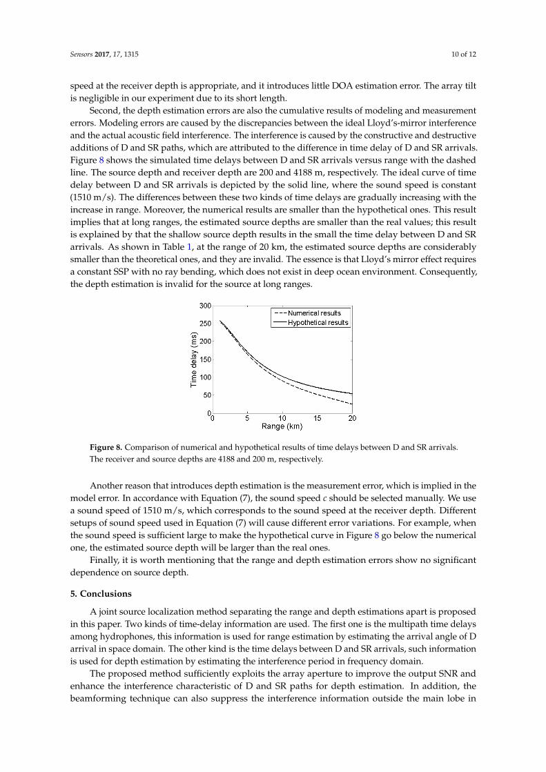
Second, the depth estimation errors are also the cumulative results of modeling and measurementerrors. Modeling errors are caused by the discrepancies between the ideal Lloyd’s-mirror interferenceand the actual acoustic field interference. The interference is caused by the constructive and destructiveadditions of D and SR paths, which are attributed to the difference in time delay of D and SR arrivals.Figure 8 shows the simulated time delays between D and SR arrivals versus range with the dashedline. The source depth and receiver depth are 200 and 4188 m, respectively. The ideal curve of timedelay between D and SR arrivals is depicted by the solid line, where the sound speed is constant(1510 m/s). The differences between these two kinds of time delays are gradually increasing with theincrease in range. Moreover, the numerical results are smaller than the hypothetical ones. This resultimplies that at long ranges, the estimated source depths are smaller than the real values; this resultis explained by that the shallow source depth results in the small the time delay between D and SRarrivals. As shown in Table 1, at the range of 20 km, the estimated source depths are considerablysmaller than the theoretical ones, and they are invalid. The essence is that Lloyd’s mirror effect requiresa constant SSP with no ray bending, which does not exist in deep ocean environment. Consequently,the depth estimation is invalid for the source at long ranges.

Sensors 2017, 17, 1315 10 of 11

than the real values; this result is explained by that the shallow source depth results in the small the time delay between D and SR arrivals. As shown in Table 1, at the range of 20 km, the estimated source depths are considerably smaller than the theoretical ones, and they are invalid. The essence is that Lloyd’s mirror effect requires a constant SSP with no ray bending, which does not exist in deep ocean environment. Consequently, the depth estimation is invalid for the source at long ranges.

Another reason that introduces depth estimation is the measurement error, which is implied in the model error. In accordance with Equation (7), the sound speed c should be selected manually. We use a sound speed of 1510 m/s, which corresponds to the sound speed at the receiver depth. Different setups of sound speed used in Equation (7) will cause different error variations. For example, when the sound speed is sufficient large to make the hypothetical curve in Figure 8 go below the numerical one, the estimated source depth will be larger than the real ones.

Figure 8. Comparison of numerical and hypothetical results of time delays between D and SR arrivals. The receiver and source depths are 4188 and 200 m, respectively.

Finally, it is worth mentioning that the range and depth estimation errors show no significant dependence on source depth.

5. Conclusions

A joint source localization method separating the range and depth estimations apart is proposed in this paper. Two kinds of time-delay information are used. The first one is the multipath time delays among hydrophones, this information is used for range estimation by estimating the arrival angle of D arrival in space domain. The other kind is the time delays between D and SR arrivals, such information is used for depth estimation by estimating the interference period in frequency domain.

The proposed method sufficiently exploits the array aperture to improve the output SNR and enhance the interference characteristic of D and SR paths for depth estimation. In addition, the beamforming technique can also suppress the interference information outside the main lobe in multiobjective scenes. However, at long ranges, Lloyd’s mirror principle does not work well, and the depth estimation error is large. Experimental results using explosive sources exhibit acceptable localization results. The proposed method can be used for the bottom-deployed VLA for underwater autonomous unmanned alerting due to its operation simplification and performance stability for near-range source localization.

Acknowledgments: This work was supported by the National Natural Science Foundation of China under Grant 11174235.

Author Contributions: Kunde Yang conceived and designed the experiments; Hui Li and Kunde Yang performed the experiments; Rui Duan and Zhixiong Lei analyzed the data; Rui Duan participated in the detailed analysis of the results; Hui Li wrote the paper.

Conflicts of Interest: The authors declare no conflict of interest.

References

Figure 8. Comparison of numerical and hypothetical results of time delays between D and SR arrivals.The receiver and source depths are 4188 and 200 m, respectively.

Another reason that introduces depth estimation is the measurement error, which is implied in themodel error. In accordance with Equation (7), the sound speed c should be selected manually. We usea sound speed of 1510 m/s, which corresponds to the sound speed at the receiver depth. Differentsetups of sound speed used in Equation (7) will cause different error variations. For example, whenthe sound speed is sufficient large to make the hypothetical curve in Figure 8 go below the numericalone, the estimated source depth will be larger than the real ones.

Finally, it is worth mentioning that the range and depth estimation errors show no significantdependence on source depth.

5. Conclusions

A joint source localization method separating the range and depth estimations apart is proposedin this paper. Two kinds of time-delay information are used. The first one is the multipath time delaysamong hydrophones, this information is used for range estimation by estimating the arrival angle of Darrival in space domain. The other kind is the time delays between D and SR arrivals, such informationis used for depth estimation by estimating the interference period in frequency domain.

The proposed method sufficiently exploits the array aperture to improve the output SNR andenhance the interference characteristic of D and SR paths for depth estimation. In addition, thebeamforming technique can also suppress the interference information outside the main lobe in

Sensors 2017, 17, 1315 11 of 12

multiobjective scenes. However, at long ranges, Lloyd’s mirror principle does not work well, andthe depth estimation error is large. Experimental results using explosive sources exhibit acceptablelocalization results. The proposed method can be used for the bottom-deployed VLA for underwaterautonomous unmanned alerting due to its operation simplification and performance stability fornear-range source localization.

Acknowledgments: This work was supported by the National Natural Science Foundation of China underGrant 11174235.

Author Contributions: Kunde Yang conceived and designed the experiments; Hui Li and Kunde Yang performedthe experiments; Rui Duan and Zhixiong Lei analyzed the data; Rui Duan participated in the detailed analysis ofthe results; Hui Li wrote the paper.

Conflicts of Interest: The authors declare no conflict of interest.

References

1. Thompson, S.R. Sound Propagation Considerations for a Deep-Ocean Acoustic Network. Master’s Thesis,Naval Postgraduate School, Monterey, CA, USA, 2009.

2. Duan, R.; Yang, K.; Ma, Y.; Lei, B. A reliable acoustic path: Physical properties and a source localizationmethod. Chin. Phys. B 2012, 21, 124301. [CrossRef]

3. Baggeroer, A.B.; Scheer, E.K.; Heaney, K.; Spain, G.D.; Worcester, P.; Dzieciuch, M. Reliable acoustic path andconvergence zone bottom interaction in the Philippine Sea 09 Experiment. J. Acoust. Soc. Am. 2010, 128, 2385.[CrossRef]

4. Duan, R.; Yang, K.; Ma, Y.; Yang, Q.; Li, H. Moving source localization with a single hydrophone usingmultipath time delays in the deep ocean. J. Acoust. Soc. Am. 2014, 136, EL159–EL165. [CrossRef] [PubMed]

5. Yang, K.; Li, H.; Duan, R.; Yang, Q. Analysis on the characteristic of cross-correlated field and its potentialapplication on source localization in deep water. J. Comp. Acoust. 2017, 25, 1750001-1–1750001-15. [CrossRef]

6. Lei, Z.; Yang, K.; Ma, Y. Passive localization in the deep ocean based on cross-correlation function matching.J. Acoust. Soc. Am. 2016, 139, EL196–EL201. [CrossRef] [PubMed]

7. McCargar, R.; Zurk, L.M. Depth-based signal separation with vertical line arrays in the deep ocean. J. Acoust.Soc. Am. 2013, 133, EL320–EL325. [CrossRef] [PubMed]

8. Kniffin, G.P.; Boyle, J.K.; Zurk, L.M.; Siderius, M. Performance metrics for depth-based signal separationusing deep vertical line arrays. J. Acoust. Soc. Am. 2016, 139, 418–425. [CrossRef] [PubMed]

9. Voltz, P.; Lu, I. A time-domain backpropagating ray technique for source localization. J. Acoust. Soc. Am.1994, 95, 805–812. [CrossRef]

10. Skarsoulis, E.K.; Kalogerakis, M.A. Ray-theoretic localization of an impulsive source in a stratified oceanusing two hydrophones. J. Acoust. Soc. Am. 2005, 118, 2934–2943. [CrossRef]

11. Jesus, S.M.; Porter, M.B.; Stephan, Y.; Demoulin, X.; Rodriguez, O.C.; Coelho, E.M.M.F. Single hydrophonesource localization. IEEE J. Ocean. Eng. 2000, 25, 337–346. [CrossRef]

12. Duan, R.; Yang, K.; Ma, Y. Narrowband source localisation in the deep ocean using a near-surface array.Acoust. Aust. 2014, 42, 36–42.

13. Baggeroer, A.B.; Kuperman, W.A.; Mikhalevsky, P.N. An overview of matched field methods in oceanacoustics. IEEE J. Ocean. Eng. 1993, 18, 401–424. [CrossRef]

14. Jensen, F.B.; Kuperman, W.A.; Porter, M.B.; Schmidt, H. Computational Ocean Acoustics; Springer: Berlin,Germany, 2011.

15. Yang, K.; Li, H.; He, C.; Duan, R. Error analysis on bearing estimation of a towed array to a far-field sourcein deep water. Acoust. Aust. 2016, 44, 429–437. [CrossRef]

16. Porter, M.B. The BELLHOP Manual and User’s Guide: Preliminary and Draft; Heat, Light and Sound ResearchInc.: La Jolla, CA, USA, 2011.

17. Sun, M.; Zhou, S.; Li, Z. Analysis of sound propagation in the direct-arrival zone in deep water with a vectorsensor and its application. Acta Phys. Sin. 2016, 65, 094302-1–094302-9.

18. Reeder, D.B. Clutter depth discrimination using the wavenumber spectrum. J. Acoust. Soc. Am. 2014, 135,EL1–EL7. [CrossRef] [PubMed]

Sensors 2017, 17, 1315 12 of 12

19. Rakotonarivo, S.T.; Kuperman, W.A. Model-independent range localization of a moving source in shallowwater. J. Acoust. Soc. Am. 2012, 132, 2218–2223. [CrossRef] [PubMed]

20. Li, Z.; Zurk, L.M.; Ma, B. Vertical arrival structure of shipping noise in deep water channels. In Proceedingsof the OCEANS 2010 MTS/IEEE, Seattle, WA, USA, 20–23 September 2010.

21. Chapman, N.R. Measurement of the waveform parameters of shallow explosive charges. J. Acoust. Soc. Am.1985, 78, 672–681. [CrossRef]

© 2017 by the authors. Licensee MDPI, Basel, Switzerland. This article is an open accessarticle distributed under the terms and conditions of the Creative Commons Attribution(CC BY) license (http://creativecommons.org/licenses/by/4.0/).