Joint Defra / Environment Agency Flood and Coastal … · This report recommends changes to the...
144
Joint Defra / Environment Agency Flood and Coastal Erosion Risk Management R&D Programme Improving the FEH statistical procedures for flood frequency estimation Science Report: SC050050 Product Code: SCHO0608BOFF-E-P
Transcript of Joint Defra / Environment Agency Flood and Coastal … · This report recommends changes to the...

Joint Defra / Environment Agency Flood and Coastal ErosionRisk Management R&D Programme
Improving the FEH statistical procedures for flood frequency estimation
Science Report: SC050050
Product Code: SCHO0608BOFF-E-P

ii Science Report – Improving the FEH statistical procedures for flood frequency estimation
The Environment Agency is the leading public body protecting and improving the environment in England and Wales.
It’s our job to make sure that air, land and water are looked after by everyone in today’s society, so that tomorrow’s generations inherit a cleaner, healthier world.
Our work includes tackling flooding and pollution incidents, reducing industry’s impacts on the environment, cleaning up rivers, coastal waters and contaminated land, and improving wildlife habitats.
This report is the result of research commissioned and funded by the Environment Agency’s Science Programme.
Published by: Environment Agency, Rio House, Waterside Drive, Aztec West, Almondsbury, Bristol, BS32 4UD Tel: 01454 624400 Fax: 01454 624409 www.environment-agency.gov.uk ISBN: 978-1-84432-920-5 © Environment Agency – June 2008 All rights reserved. This document may be reproduced with prior permission of the Environment Agency. The views and statements expressed in this report are those of the author alone. The views or statements expressed in this publication do not necessarily represent the views of the Environment Agency and the Environment Agency cannot accept any responsibility for such views or statements. This report is printed on Cyclus Print, a 100% recycled stock, which is 100% post consumer waste and is totally chlorine free. Water used is treated and in most cases returned to source in better condition than removed. Further copies of this report are available from: The Environment Agency’s National Customer Contact Centre by emailing: [email protected] or by telephoning 08708 506506.
Author(s): Thomas R. Kjeldsen, David A. Jones and Adrian C. Bayliss Dissemination Status: Released to all regions Publicly available Keywords: Flood Estimation, Extreme Values, HiFlows-UK, Index flood, Pooling-Groups, Growth Curves, Donor catchments Research Contractor: Centre for Ecology & Hydrology Maclean Building Crowmarsh Gifford Wallingford, OX10 8BB 01491 838800 www.ceh.ac.uk www.nerc.ac.uk Environment Agency’s Project Manager: Paul Webster, Hydro-Logic ltd Stefan Laeger, Environment Agency Science Department Science Project Number: SC050050 Product Code: SCHO0608BOFF-E-P

Science Report – Improving the FEH statistical procedures for flood frequency estimation iii
Science at the Environment Agency Science underpins the work of the Environment Agency. It provides an up-to-date understanding of the world about us and helps us to develop monitoring tools and techniques to manage our environment as efficiently and effectively as possible.
The work of the Environment Agency’s Science Department is a key ingredient in the partnership between research, policy and operations that enables the Environment Agency to protect and restore our environment.
The science programme focuses on five main areas of activity:
• Setting the agenda, by identifying where strategic science can inform our evidence-based policies, advisory and regulatory roles;
• Funding science, by supporting programmes, projects and people in response to long-term strategic needs, medium-term policy priorities and shorter-term operational requirements;
• Managing science, by ensuring that our programmes and projects are fit for purpose and executed according to international scientific standards;
• Carrying out science, by undertaking research – either by contracting it out to research organisations and consultancies or by doing it ourselves;
• Delivering information, advice, tools and techniques, by making appropriate products available to our policy and operations staff.
Steve Killeen
Head of Science

Science Report – Improving the FEH statistical procedures for flood frequency estimation v
Executive summary This report recommends changes to the procedures contained in the Flood Estimation Handbook (FEH), which have been adopted as standard practice by the principal bodies engaged in flood frequency estimation in the UK and, in particular, by the Environment Agency. These procedures provide estimates of the flows that will occur in rivers on moderately rare occasions: flow values that have an exceedance probability in any given year of 50 per cent (a 2-year return period) to 1 per cent (a 100-year return period), or even more rare. In the majority of cases where such estimates are required, the locations affected will be ungauged and too far from established river gauging stations to provide data records that can be immediately transferred.
The changes recommended arise, in part, because the HiFlows-UK project has led to the creation of a much-improved database of systematically recorded flood data. Not only are the data records now much longer than those used previously but the HiFlows-UK project put substantial effort into the quality control and assessment of the whole data-set. This means that the data available for analysis have been dramatically improved. Another influence on the renewed procedures has been feedback from users of the FEH, both informal and formal. Without substantially changing the overall framework of the methodology, most technical details of the method have been updated to improve the performance of the procedure. The updates include significant improvements to the theoretical statistical framework underlying the method.
In addition, it has been possible to consider some new descriptors of catchment topography and local climate that have been proposed since the FEH study. In particular, a new descriptor that measures floodplain extent has been devised and is now included in the improved procedures.
This report is largely a technical description of the studies that have led to the new recommendations. The folllowing are the key improvements.
• A new regression model for estimating the median annual maximum flood (QMED) at ungauged catchments (Chapter 4).
• An improved procedure for the use of donor catchments for estimation of QMED at ungauged catchments (Chapter 5).
• An improved procedure for formation of pooling groups and estimation of pooled growth curves (Chapter 6).
Flood estimates produced by the new procedures can be substantially different from those produced using the original FEH procedures. On taking the catchments whose data have been analysed as typical examples, and treating them as if they were ungauged, the ratios of the new estimates to the FEH estimates indicate the following changes.
• The changes in QMED range from 0.55 to 2.01, with half being greater than 1.15 (25 per cent of the ratios are less than 1.00, and 25 per cent are greater than 1.24).
• For floods with an annual probability of exceedance of 1 per cent (the 1 per cent flood), the changes range from 0.48 to 2.24, with half being greater than 1.14 (25 per cent of the ratios are less than 0.97 and 25 per cent are greater than 1.32).
For both QMED and the 1 per cent flood, the new procedure produced lower estimates than the FEH in the East of England, whereas increases in both quantities were generally observed in West England, Wales and Scotland.

vi Science Report – Improving the FEH statistical procedures for flood frequency estimation
Acknowledgements The Centre for Ecology and Hydrology (CEH) project team wishes to acknowledge the following people and organisations for assistance provided during the project:
• The Environment Agency HiFlows-UK project for making available the HiFlows-UK data set of annual maximum peak flow and peaks-over-threshold series.
• The Project Steering Group: Paul Webster (Hydro-Logic Ltd), David MacDonald (Black & Veatch), Peter Spencer (Environment Agency), and Kate Marks (Environment Agency).
• Reviewers of the draft report: The Project Steering Group, Stefan Laeger (Environment-Agency), Rob Lamb (JBA Consulting), Duncan Faulkner (JBA Consulting), and Eleanor Heron (Environment Agency).
• Colleagues at CEH, in particular Lisa Stewart and David Morris.

Science Report – Improving the FEH statistical procedures for flood frequency estimation vii
Contents 1 Introduction 1 1.1 Statistical flood frequency estimation in the UK 1 1.2 Why is an update needed? 4 1.3 Outcome of the present study 5 1.4 Structure of the report 6
2 Appraisal and selection of data 7 2.1 Flood peak data 7 2.2 Catchment descriptors 10
3 Floodplain descriptors 14 3.1 Choice of data 14 3.2 Revision of IH130 flood depth data 15 3.3 Key characteristics 16 3.4 Definition of the descriptors 16 3.5 Deriving descriptor values 17 3.6 The FPEXT, FPLOC and FPDBAR data 17
4 Improving QMED estimation 21 4.1 Review of previous models (QBAR and QMED) 21 4.2 QMED estimation at gauged sites 23 4.3 Regression model description 26 4.4 Variable selection 31 4.5 Estimating a new QMED model 35 4.6 Comparison between the new model and the FEH model 38
5 Use of donor sites 42 5.1 FEH donor adjustment 42 5.2 New data transfer scheme 42 5.3 Using the network structure 43 5.4 Performance 44 5.5 Discussion of data transfer 46 5.6 Example: donor transfer 46
6 Improving the FEH pooling procedure 51 6.1 Pooled frequency analysis 52 6.2 Performance measure 53 6.3 Formation of pooling-groups 54 6.4 Weight of L-moments within pooling-groups 56 6.5 Size of pooling-groups 62 6.6 Performance of pooling-groups 64

viii Science Report – Improving the FEH statistical procedures for flood frequency estimation
6.7 Example: a pooling-group 66 6.8 Comparison of results for 100-year return period 74
7 Default distribution 79 7.1 The Hosking and Wallis test 79 7.2 Revision of the Hosking and Wallis test 80 7.3 The test procedure 81 7.4 Results 82
8 Summary of new flood estimation procedures 84 8.1 Estimation of QMED 84 8.2 Estimation of the growth curve 85 8.3 Estimation of the flood frequency curve 88
9 Conclusions 89 9.1 Improved modelling techniques 89 9.2 HiFlows-UK 90 9.3 Future direction of research and development 90
References 95
Appendix A QMED values and gauge details 98
Appendix B FPEXT, FPLOC and FPDBAR values 111
Appendix C GLS regression details 125
Appendix D Details of weighting scheme 128
Glossary 133
List of Symbols 136

Science Report – Improving the FEH statistical procedures for flood frequency estimation 1
1 Introduction
This report presents the results of the R&D project SC050050 Improving the FEH statistical procedures for flood frequency estimation, funded by the Joint Department for Environment, Food and Rural Affairs (Defra)/Environment Agency Flood and Coastal Erosion Risk Management R&D Programme.
1.1 Statistical flood frequency estimation in the UK The use of statistical extreme value techniques for flood frequency analysis is a long-established practice in applied hydrology, both in the UK and elsewhere. This section sets the research conducted in the present project in context with regard to the developments of this particular branch of hydrology. For the UK, two key milestones were the Flood Studies Report (FSR) published by the Natural Environment Research Council (NERC, 1975) and the Flood Estimation Handbook (FEH) (Institute of Hydrology, 1999). The hydrological literature contains a vast number of references to the application of various statistical distributions to model annual maximum (AMAX) series of peak flow and, due to the subject’s importance, this literature is constantly growing.
1.1.1 Pre-FSR
An excellent overview of the state of flood frequency analysis in the UK before the publication of the FSR was provided by Wolf (1965), who traced the use of statistical methods in flood frequency analysis back to the early 20th century (Gore and Thomson, 1909; Horton, 1913, both cited by Wolf, 1965). However, the first systematic application of extreme value theory and models in hydrology is often attributed to Gumbel (1941), who successfully fitted extreme value distributions of Type 1 (Gumbel distributions) to AMAX series of daily mean flow from many countries. Other methodological milestones of importance to the subsequent development of national UK procedures include the publication of the Generalised Extreme Value (GEV) distribution (Jenkinson, 1955) and the development of the index-flood method at the United States Geological Survey (USGS) reported by Dalrymple (1960).
1.1.2 Flood Studies Report
The Flood Studies Report (FSR) provided the first unified framework for conducting flood frequency analysis at both gauged and ungauged catchments in the UK, and it has been instrumental in the continued development of flood frequency methodologies worldwide. The FSR procedure is based on the index-flood method, where a flood frequency curve is represented by the product of the following two elements.
• An index flood, defined as the mean annual maximum flood (QBAR).
• A dimensionless growth curve, derived through the fitting of a GEV distribution to normalised AMAX data within a specified geographical region.
The FSR divided the British Isles into eleven different regions and estimated a growth curve for each region as shown in Figure 1.1.

2 Science Report – Improving the FEH statistical procedures for flood frequency estimation
Figure 1.1 Geographical regions and the associated growth curves for flood frequency analysis in the UK, as defined by the FSR (From Sutcliffe, 1978).
The individual growth curves were fitted to the regional data by manually adjusting the growth curve parameters. As well as growth curves, the FSR provided a set of regression models for predicting the index flood in each region. The regression models linked QBAR to a set of catchment characteristics which a user would need to obtain from both Ordnance Survey and FSR thematic maps. The catchment characteristics required were the following nine variables: AREA, MSL, S1085, STMFRQ, SOIL, LAKE, URBAN, SAAR and RSMD,
Subsequent research by Hosking et al. (1985) suggested that the algorithm used to derive a FSR growth curve for a given catchment did not perform as well as a new procedure which was still based on the GEV distribution, but which derived the growth curve by using probability-weighted moments (PWM), as described by Wallis (1981). Some researchers developed methods allowing the FSR approach to be used for dealing with flood frequency analysis in urban areas (Packman, 1980) while others placed an increased focus on the use of data transfer from gauged (donor) catchments to ungauged catchments as a possible method for enhancing estimates at the ungauged catchments (Institute of Hydrology, 1983).
1.1.3 Flood Estimation Handbook (FEH)
Rather than dissatisfaction with the performance of the FSR method, it was methodological developments in regional flood frequency analysis that led to a re-evaluation of the FSR methodology as presented in the FEH. In particular, two developments that have been influential both in the UK and elsewhere are the seminal

Science Report – Improving the FEH statistical procedures for flood frequency estimation 3
work by Hosking and Wallis (1997), who popularised the L-moment approach to regional frequency analysis, and the introduction of the region of influence (ROI) approach by Burn (1990).
In the time that passed between the publication of the FSR and the onset of the FEH development, advances in digital mapping techniques, statistics and hydrological modelling combined with the widespread availability of desktop computing to make the development of new system for flood estimation possible. This was a more flexible but, at the same time, a more complex and computationally burdensome system than the FSR. While retaining the index-flood method as the basis of the procedure, the FSR method of dealing with the growth curve component using geographical regions was replaced in the FEH by the concept of pooling-groups. Here, for each site of interest, a unique ‘region’ (pooling-group) is created based on ‘hydrological similarity’. The pooling-group for a given site of interest was defined by searching a database of 1,000 potential sites to find catchments judged to be ‘hydrologically similar’. This judgement was based on similarity of catchment area (AREA), annual average rainfall (SAAR) and hydrological soil properties as defined by the HOST classes (BFIHOST). An example of a pooling-group is shown in Figure 1.2.
Figure 1.2 Example of a subject site (red cross) and the most hydrologically similar gauged catchments (black squares) included in the FEH pooling-group.
The use of fixed geographical regions had been criticised for pooling together data from catchments with very different sizes and soil types (Institute of Hydrology, 1999), as well as being counter-intuitive when a particular site of interest is located close to the border between two geographical regions. While the pooling approach addresses both these problems, it should be noted that there may be locations with catchment characteristics outside the normal range of values that might still be perceived as being

4 Science Report – Improving the FEH statistical procedures for flood frequency estimation
lon a boundary (i.e. be adjacent to an empty region in catchment descriptor space). In comparison to using geographical space, such a boundary problem might not be as easily identified.
The FEH changed the index flood from the mean annual flood (QBAR) to the median annual flood (QMED), as the latter was considered to be more robust to outliers in short series. A single regression model linking the QMED to a set of six catchment descriptors was developed for general use in the UK. The resulting equation is often referred to as ‘the QMED equation’. Additional calculation steps were introduced with the aim of improving the estimates from the QMED equation by making use of information at gauged sites that were either geographically close or judged to be hydrologically similar to the target catchment (termed donor and analogue catchments, respectively).
The FEH also recommended that the Generalised Logistic (GLO) distribution, rather than the GEV distribution, should be adopted as default distribution in the UK.
A key advance in the FEH was the use of digitally derived catchment descriptors and the release of the accompanying FEH CD-ROM. The digital catchment descriptors replaced the catchment characteristics that previously had to be derived manually from maps.
1.1.4 Post-FEH
A comprehensive assessment of the FEH statistical method was reported by Morris (2003) based on results obtained by generalising the method to the entire river network in the UK. Many of the recommendations made by Morris to improve the FEH have been addressed in the work undertaken in this project.
More recently, a series of publications by Kjeldsen and Jones (2006, 2007, 2008) have identified the link between the model error structure of the QMED regression model and the benefit obtained from the use of data transfer from donor and analogue catchments. The results of these studies have informed the development of both the new QMED equation and the revised data transfer procedure presented in this study.
1.2 Why is an update needed? While the FEH has served the hydrological community well, the additional ten years of peak flow data generated by the HiFlows-UK project (see Table 2.1) needs to be taken into account. In addition to the extended record lengths, the HiFlows-UK project put substantial effort into reconsidering the level-discharge rating curves, general quality control and assessing the reliability of the data-records. Given that the new database provides substantially longer records while enabling the avoidance of poor-quality data, an update of the FEH procedures was considered necessary.
This project also provides an opportunity to disseminate the result of research into flood frequency analysis, undertaken at the Centre for Ecology and Hydrology (CEH) since the publication of the FEH in late 1999.

Science Report – Improving the FEH statistical procedures for flood frequency estimation 5
1.3 Outcome of the present study As outlined above, the present study has examined a number of aspects of the FEH methodology. Details of these analyses are given in later chapters. In order to provide an indication of the scope of this work, Table 1.1 provides a summary of the recommendations being made as a result of this project
Table 1.1 Recommendations from the present study.
Component of FEH methodology
Recommendations Comments
QMED equation. Equation using revised set of catchment descriptors.
• Fitted to updated data-set. • Improved representation of relation to catchment descriptors. • Outperforms the FEH equation.
Using gauged data to adjust initial estimate of QMED.
• Discontinue use of “analogue” (hydrologically similar) catchments. • Weight donor catchments using geographical distance.
• Adjustments based on FEH donor catchments likely to make estimates worse. • New donor scheme Improves estimates of QMED.
Pooling-groups: selection of similar catchments.
New set of catchment descriptors used to measure hydrological similarity.
Includes a new catchment descriptor for floodplain extent not available for FEH.
Pooling-groups: weighting within pooling-group.
• New weighting scheme making direct use of both a new measure of hydrological similarity and record lengths. • Explicit treatment of case where target catchment is gauged.
• New weights avoid pitfalls in FEH formulation as noted by users. • FEH used the same weights for both gauged and ungauged subject catchments. • Improved performance demonstrated.
Default distribution. Retain GLO as default. Assessment based on improved methodology and gave same conclusion as FEH.
Catchment descriptors. • Digital data-sets for new descriptors constructed, most importantly for flood plains. • Possible usefulness of new descriptors assessed throughout procedures.
New flood plain descriptor contributes to revised pooling-group methodology.

6 Science Report – Improving the FEH statistical procedures for flood frequency estimation
1.4 Structure of the report This report presents the results of the analysis undertaken as part of the current project.
Chapter 2 contains a summary of the data used in this study, both flood data and catchment descriptor data.
Chapter 3 details the development of a new range of catchment descriptors quantifying the extent of floodplains in the catchment.
Chapter 4 presents the development of a new QMED equation.
Chapter 5 introduces a new procedure for data transfer from gauged donor sites to an ungauged target site.
Chapter 6 presents the new procedure for forming pooling-groups and estimating the pooled growth curve.
Chapter 7 is concerned with finding a suitable distribution type for use as the default distribution in the UK.
Chapter 8 provides a short summary of the findings of this study and how the new procedure relates to the existing FEH statistical procedure.
Chapter 9 presents the general conclusions of the project and outlines some ideas as to how research into statistical methods for flood frequency estimation might be progressed in future.
Appendices A and B provide details of the data used for this study.
Appendices C and D provide mathematical details that were not appropriate in the main text.

Science Report – Improving the FEH statistical procedures for flood frequency estimation 7
2 Appraisal and selection of data
The development of statistical models for flood frequency analysis requires two types of data: i) observed flood peak data, and ii) data on physical catchment descriptors. The following sections describe the data that have been collected and analysed in this study. This study also developed a new set of catchment descriptors measuring the extent of floodplains and washlands in catchments. The details of how these descriptors were derived are reported in Chapter 3.
2.1 Flood peak data Two types of flood peak data have traditionally been used in statistical flood frequency analysis: annual maximum (AMAX) series and peaks-over-threshold (POT) series of instantaneous flow. AMAX series consist of the largest value observed within each water-year, whereas POT series consist of the peak flow of all independent peaks exceeding a specified threshold. A comprehensive review of how to extract these flow series was provided as part of the FEH (see Vol.3, Chapter 23) and is not repeated here. Both the AMAX and POT series used in this study were obtained from the HiFlows-UK project. The final water-year in the flow series available for the present project is 2002 (October 2002 to September 2003).
2.1.1 Annual maximum series
The HiFlows-UK database contains AMAX series from 962 gauging stations located throughout the UK. Initial screening of the data, combined with further amendments received from the HiFlows-UK team, and liaison with scientific staff at the National River Flow Archive (NRFA) introduced a number of corrections to the initial data set. Further adjustments were made based on anomalies identified as part of the subsequent modelling of the data.
A total of 112 records were found to be unsuitable for use in this project. The majority of these records had already been identified by the HiFlows-UK team as unsuitable for estimation of QMED and unsuitable for inclusion in a pooled analysis. A further 42 gauges were discarded as no suitable set of catchment descriptors could be identified. (Note that similar cases arose in the FEH study.) These exceptional cases relate to catchments where the catchment-areas calculated from the present version of digital map information have an unacceptable disagreement with the areas generally accepted for those catchments. Finally, 206 gauges were omitted from the analysis as the degree of urbanisation on these catchments was sufficiently high (URBEXT2000 > 0.030) for them to be considered non-rural. For a more in-depth discussion of the revised definition of an urban catchment using URBEXT2000 compared to that used in FEH, please refer to Bayliss et al. (2006).
The following paragraphs summarise some quantitative differences between the updated data set and that used in the FEH. As well as these differences, one should recall that the HiFlows-UK project attempted a coordinated quality-control assessment of the data, including an assessment of the rating curves. There is therefore an expectation that the dataset analysed here will be of a higher reliability than that available for the FEH.

8 Science Report – Improving the FEH statistical procedures for flood frequency estimation
Figure 2.1 Location of 602 gauging stations on rural catchments providing instantaneous annual maximum flood peak data.
The final data set consisted of 602 rural catchments. The locations of the gauging stations are shown in Figure 2.1. Appendix A provides details of these 602 catchments. A summary of the data-set is shown in Table 2.1. The statistical methodology established in the FEH project was based on a total of 728 rural catchments, 126 more than used in this study.
0
0
100000
100000
200000
200000
300000
300000
400000
400000
500000
500000
600000
600000
700000
700000
0 0
100000 100000
200000 200000
300000 300000
400000 400000
500000 500000
600000 600000
700000 700000
800000 800000
900000 900000
1000000 1000000
Science Report – Improving the FEH statistical procedures for flood frequency estimation 9
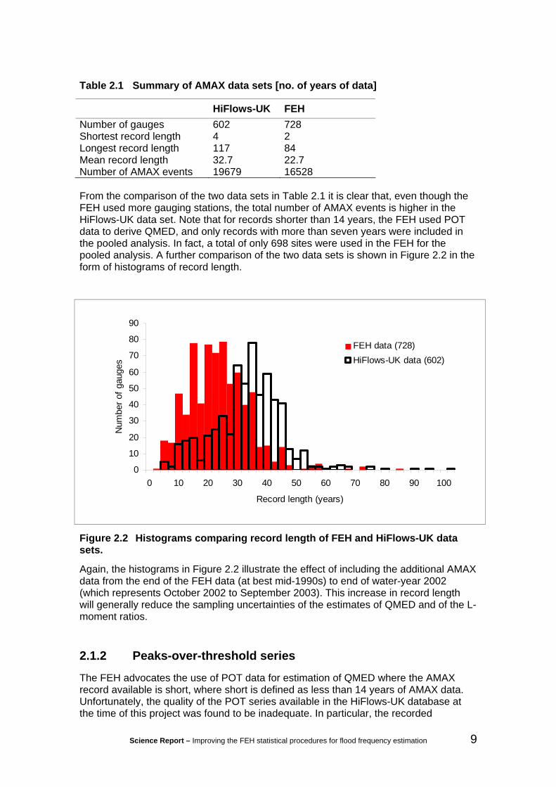
Table 2.1 Summary of AMAX data sets [no. of years of data]
HiFlows-UK FEH Number of gauges 602 728 Shortest record length 4 2 Longest record length 117 84 Mean record length 32.7 22.7 Number of AMAX events 19679 16528 From the comparison of the two data sets in Table 2.1 it is clear that, even though the FEH used more gauging stations, the total number of AMAX events is higher in the HiFlows-UK data set. Note that for records shorter than 14 years, the FEH used POT data to derive QMED, and only records with more than seven years were included in the pooled analysis. In fact, a total of only 698 sites were used in the FEH for the pooled analysis. A further comparison of the two data sets is shown in Figure 2.2 in the form of histograms of record length.
0
10
20
30
40
50
60
70
80
90
0 10 20 30 40 50 60 70 80 90 100
Record length (years)
Num
ber o
f gau
ges
FEH data (728)HiFlows-UK data (602)
Figure 2.2 Histograms comparing record length of FEH and HiFlows-UK data sets.
Again, the histograms in Figure 2.2 illustrate the effect of including the additional AMAX data from the end of the FEH data (at best mid-1990s) to end of water-year 2002 (which represents October 2002 to September 2003). This increase in record length will generally reduce the sampling uncertainties of the estimates of QMED and of the L-moment ratios.
2.1.2 Peaks-over-threshold series
The FEH advocates the use of POT data for estimation of QMED where the AMAX record available is short, where short is defined as less than 14 years of AMAX data. Unfortunately, the quality of the POT series available in the HiFlows-UK database at the time of this project was found to be inadequate. In particular, the recorded

10 Science Report – Improving the FEH statistical procedures for flood frequency estimation
information concerning start and end dates was generally poor, as was the recording of periods of missing data. The decision was therefore made not to use POT data in this project. Because of the relatively long data series in HiFlows-UK, only a relatively small percentage of stations were affected by this decision.
2.2 Catchment descriptors The digital catchment descriptors used in this study were mainly extracted from the FEH CD-ROM Version 2 (CEH, 2007) for each of the 602 gauged catchments. The number of catchment descriptors potentially available is large, but only a subset of variables previously found to be useful in flood studies were included in this study. In addition to the existing descriptors available from the FEH CD-ROM, a series of additional descriptors were developed for this project. These are as follows.
• The extent of floodplains (FPEXT, FPBAR, FPLOC).
• The steepness of design rainfall growth curves (PRAT).
• The annual evaporation (EVAP).
The last two were easily derived from data-sets already available, while the floodplain descriptors required more work. A comprehensive description of the floodplain descriptors is the focus of the next chapter, while the other two descriptors are described in this Section (2.2.2-3). It should be noted that the SPRHOST descriptor is not included in the final set of descriptors used for this study (Table 2.2). Instead, BFIHOST is used as a measure of hydrological soil properties. The BFIHOST descriptor is considered more reliable (Kjeldsen et al., 2005) as it is derived from a significantly larger data set than SPRHOST. When SPRHOST was considered as a candidate variable for modelling purposes, it provided no extra benefit once use had been made of BFIHOST.
Table 2.2 Summary of catchment descriptors used in this study
Descriptor name Unit Range Note AREA km2 [0;∞[ Catchment area as defined by DTM. SAAR mm [0;∞[ Standard annual average rainfall 1961-1990. FARL [0;1] Index of flood attenuation due to reservoirs
and lakes. BFIHOST [0;1] Baseflow index derived from HOST data. PROPWET [0;1] Proportion of time when soil moisture deficit
≤ 6 mm during 1961-90, defined using MORECS.
DPSBAR m.km-1 [0;∞[ Mean catchment slope. FPEXT [0;1] Floodplain extent. PRAT [0;∞[ Ratio between P100 and P2 for 1-day rainfall
(FEH DDF model). RMED(1day) mm [0;∞[ Median annual maximum 1-day rainfall
(derived using FEH DDF model). EVAP mm [0;∞[ Average annual potential evaporation.
A summary of the catchment descriptors for the 602 catchments is given in Table 2.2. Note that the values used in the FEH project were directly equivalent to those included in Version 1 of the FEH CD-ROM and are therefore likely be less reliable than the values used in this study. Relevant improvements to the data in the upgrade from

Science Report – Improving the FEH statistical procedures for flood frequency estimation 11
Version 1 to 2 will have been derived from improved catchment boundary and drainage path definitions: these form the basis of all the catchment descriptors.
All variables were screened by plotting against QMED (all in log-space) to check for outliers, non-linear relationships and for possible cross-correlation between the descriptors. Figure 2.3 shows a matrix of scatter plots of the catchment descriptors and it also includes the cross-correlations between the descriptors. Figure 2.4 is intended as a guide to the interpretation of Figure 2.3.
2.2.1 Adjustment of FARL values
The FARL values available from the FEH CD-ROM Version 2 relate to a fixed time-point determined by the reservoirs and lakes present in the underlying data set, which represents the current catchment configuration. However, some flood peak data may have been gauged during a period prior to the construction of a particular reservoir. It has therefore been necessary to adjust the initial FARL values to a set of values that represents the actual FARL values experienced during the period of recording. In some cases where the AMAX record spans a period from before and after the construction of a reservoir, part of the record was removed to obtain an AMAX record associated with a representative FARL value.
2.2.2 Steepness of design rainfall growth curves
The ratio between the 100-year and the 2-year rainfall (PRAT) is used in this project as a measure of the steepness of the design rainfall growth curve. Values have been calculated for each catchment under consideration using the FEH DDF model for rainfall frequencies. From Equations (2.2) to (2.4) in FEH Vol.2 (Faulkner, 1999), it is possible to derive the ratio between the 100- and 2-year design rainfall depths (for any duration) as
( ) ( ) ( )[ ]210021002
100 lnexp yyEDyyCP
P−+−==PRAT . (2.1)
Here PT is rainfall depth for return period T, D is rainfall duration, yT is the Gumbel reduced variate and both C and E are catchment average FEH DDF model parameters. In his appraisal of the FEH statistical method, Morris (2003, see page 113, line 5-7) stressed that any catchment descriptor reflecting the rainfall growth factors should reflect the relationship between the duration of flood-producing rainfall and catchment size. To allow for this, the descriptor PRAT was calculated based on 24-hour rainfall.
2.2.3 Annual evaporation
The opportunity to explore the value of potential evaporation (PE) as an explanatory value arose from the availability of a grid of PE values at CEH. This is based on a preliminary map of annual average total PE for short grass produced by the Met Office for previous studies. While evaporation might be used as a ‘stand alone’ variable, there is also the possibility that it might be useful in combination with SAAR so as to create a crude measure of “surplus rainfall”. Catchment-average values of PE have been derived for the catchments in the calibration data set. Evaporation was not considered as part of the FEH, but it has been found to be a useful predictor in a regression model linking QMED to catchment descriptors in south-east Australia (Rijal and Rahman, 2005).

12 Science Report – Improving the FEH statistical procedures for flood frequency estimation
lnQMED
2 4 6 8
++++
++++
+
++
+++
++++
++
+++
+++
++++++++
+
+++++
++++
+++
+++ +++ +
+++++
+
++++
++++
+
++
++++++
+
+++++
+ +++
+
++++++
+
+
++++
+++
++++
+++
+++
++
+++
++
++
+
++
++
++++
+
+++++
+
++
+
+
++++ +
++++++
+++
+
++
++++
++++
++
++++++
+++
+
+ ++
++++
++++++
+
++
+
+
+
+
+
++++
+++
++
++++
++
++
+++
+
++++++++++
+++
+
+
++
+++
++
++
+
+
+
++++++++++
+
+ +++
+
++
+
++++
++++
+
++
+
+
+
++++++
++
+++ +
++
++
+
++++++++
++
++
+
+
+++
+
+++
++
+++
++
+++
++ +++++++
+
+++
+
+++
++
+
+++
+
+++
++++++++++++
+++ ++
++++
+
++
++++
+
++++ +
++
++
+
++
+++
+
+++
+
++
++++
+
+++
+
+
++
+ +++
+
+
++
+
++++
++
+++
+++++
+++
+++ ++
+++
+
++++
+++
++
++
+
++
++
++
++++
++
+
+
+
+
++++
+
+++++++
++++
+++
+++++
++
++++
++
+
+
++++
+
+
++++ +
+
++++
+++++
+++
++
+++
++
++
++
++++ ++
+
+ ++++
++
+++++++
+++ ++++
++
+++
++++++++
++
++++
++
++
++ +++ ++
+
+
++
+++
++++
++++
+
+++
+++++++++
+++++++
++
+++
++ + ++ ++
+++++
+
+++ +
++++
+
++
+++ +++
+
++++ +
+++ ++
++++++
+
+
++++
++ +++++
++ +
+ ++
++
++ +
++
++
+
++
++
++++
+
+++++
+
++
+
+
+++++
++++++
++ +
+
++
++++
++++
++
+++++
+
+++
+
+++
++++++++++
+
++
+
+
+
+
+
+++++++
++
++++++
++++++
+++++++++++++
+
+
++
+++++
++
+
+
+
+++
+++++++
+
++++
+
+++
++++
++++
+
++
+
+
+
++++++++
++++
++++
+
++++++ ++
+++++
+
+++
+
++++
+
++
++++
++++ +++++
++
+
+++
+
+++
++
+
++++
++++
+ ++++++++
+ +++++ +++
++
+
++
+ ++
+
+
+++ ++
++
++
+
+++
++
+
+ ++
+
++
++++
+
+++
+
+
++
+++++
+
++
+
++
+++++
++++++
+
++
++
+++ +
++
+
+
+++
++
++
++
+++
+++
+++
+++++++
+
+
+
++
++
+
++ +
+++ +
++++
++++++++
++
+++
++
++
+
+ ++++
+
++++++
++++
++++
+++++
+
+++
++
++
++
++ ++++
+
+++
+ ++
++++++
+++++++
++++++
+
++++++++
++
+++++ +
++
−1.5 −0.5
++++++++
+
++
+++
+++++
++++
+++
+++++++++
+++++
++++
+++
+++++++
+++++
+
++++
+++++
++
++++++
+
+++ ++
+ +++
+
++++
++
+
+
++++
+++++++
+++
+++
++
+++
++
++
+
++
++
++++
+
+++++
+
++
+
+
+++ + +
+++ +++
+++
+
++
++++
++++
++
++ +
+++
+++
+
+ ++
+++
++ ++ ++
+
+
++
+
+
+
+
+
+++++ ++
++
++++
++
+++++
+
++++++ +++++++
+
+
++
+++
++
++
+
+
+
+++
++ +++ ++
+
+++ +
+
++
+
++++
++++
+
++
+
+
+
++++++++
++++
++
+ +
+
++++++++
+++++
+
++ +
+
++++
+
++
++
++
+ ++++++ +++ +
+
+++
+
++ +
++
+
++
++
++++
+++++++++++
+++++++++
+
++
++++
+
++++ +
+ +
++
+
+++
+ +
+
+++
+
++
++++
+
++ +
+
+
++
+++++
+
+++
+++++
++++
+++++
++++++ ++
++
+
+
++
+++
+ +
++
+++
++
++
+ +
+++++++
+
+
+
+++
++
+++
++++
++++
+++++
+++++
+++++
++
+
+++++
+
++ ++++
+ ++++
++ ++
++++
+
+++
++
++
+++++
+++
+
+++
+++
++ ++++
+++
+++ +++
++++
+
+++++++
+
++
+++ +
++
++
++ +++++
+
+
++
+++
++ ++++
+ ++
+++
+++++++++
++++ +
++++
+++
++++ + ++
+++++
+
++++
+++ +
+
++++++++
+
++++++++++
++++
++
+
+
++++
+++++++
+++
+++
++
+++
++
++
+
++
++
++++
+
++++
+
+
++
+
+
+++++
+ +++++
+++
+
++
++++
++++++
+++
+++
+++
+
+++
+ +++++ ++++
+
++
+
+
+
+
+
++++
+++
++
++++++
++++++
++++++ +++++++
+
+
+++++++
++
+
+
+
++++++ ++++
+
++++
+
+++
++++
++++
+
++
+
+
+
++++++++
++++
++
+ +
+
++++++++
++++
+
+
++++
+++++
+++
++++++++++++++
+
++ +
+
+++
++
+
++++
+++++++++++++++
+ +++
+++++
+
++
+++
+
+
+++++
++
++
+
+++
+ +
+
+++
+
++
++++
+
++++
+
++
+++
++
+
+++
++++++++++++++
++
++
+ +++
+++
+
++
+++++
++
+++
++
++++
+++++++
+
+
+
++
+++
+++
+ +++
+++ +
+++
+++ ++
++
+++
++++
+
++++
+
+
++++++
++++
++++
++++++
+++
++
++
++
+ ++++ +
+
+++
+++
++ ++++
+ ++++++++++++
+
++++++++
++
++++
+ +
++
−1.4 −0.8 −0.2
++ +++ ++
+
+
++
+++
++++
+++++
++
+
+ ++++++++
+++++++
++
+++
++++++++++++
+
+++ +
++++
+
++
+++ +++
+
++++ +
+++ ++
++++++
+
+
++++
++ +
++++
++ +
+++
++
++ +
++
++
+
++
++
++++
+
+++++
+
++
+
+
++ +++
+ +++++
++ +
+
++
++++
++++
++
+++++
+
+++
+
+++
+++
++++++
+
+
++
+
+
+
+
+
++++++
+
++
+++++
+
++++
++
+++++++++++++
+
+
+++++++
++
+
+
+
++++++++++
+
++++
+
+++
++++
++++
+
++
+
+
+
++++++++
++++
++++
+
++++++ ++
++
++
+
+
++++
+++++
+++++++++++++++
++
+
+++
+
+++
++
+
++++
+++
++ +++
++++++++++++++++
+
++
+ +++
+
+ ++ ++
++
++
+
+++
++
+
+ ++
+
++
++++
+
++++
+
++
+++++
+
++
+
++
+ ++++
++++++
+
++
++
+++ +
++
+
+
++
+++
++
++
+++
++++
++
+++++++
+
+
+
++
+++
+++++++
++++++
++++++++
+++++++
+
+++++
+
++++++
++++++++
++
++++
+++
++++
++
++++++
+
+++
+++
+++++++++++++
+++
+++
+
++++++++
++
++++++
++
++ +++ +++
+
++
+++
++++++++
+
++
+
++++++++
+
+++++++
++
+++
+++++++
+++++
+
+++ +
++++
+
+++++ +
++
+
++++ +
++++
+
++++
+ +
+
+
++++
+++++++
+++
+++
++
+++++
++
+
++
++
++++
+
++++
+
+
++
+
+
++ +++
++++++
++ +
+
++
++++
++++
++
+++
+++
+++
+
+++
+++
+++ +++
+
+
++
+
+
+
+
+
++++++
+
++
++++++
++
+ +++
+++++++++++++
+
+
++
+++++
+ +
+
+
+
+++
++ +++++
+
+++ +
+
++
+
++
++
++++
+
++
+
+
+
+++++++
+
++ ++
++++
+
++++++ ++
++
+++
+
++++
+++++
++
++++++
+++++++++
+
+++
+
+++
++
+
++++
+ ++
++ +++
++++++ +
+ ++++
++++
+
++
+++
+
+
+ ++ ++
++
++
+
+++
+ +
+
+ ++
+
++
++++
+
++++
+
++
+++++
+
++
+
++
+ ++++
++++++
+
++
++
++++
+++
+
++
++++ +
++
+++
++
++
++
+++++++
+
+
+
++
+++
++ +
++++
++++++++++++++
+++
++
++
+
+ ++++
+
+++++
+
++++
+++++
++++
+
+++
+++
+
++++ +
+++
+
+++
+ ++
++ ++++
+ ++++++
+++
+++
+
++ +++ +++
+++
++++ +
++
0.00 0.10 0.20
++++++++
+
++
+++
+++ +++
+++
+++
+++ +++++
+
+++++++
+ +
+++
+++
+++++++++
+
++++
+++++
++++++++
+
++ +++
+ ++++
+++ +++
+
+
++++
+++
++++
+++
+++
++
+++
+ +
++
+
++
++
++ ++
+
++++
+
+
++
+
+
++++ +
+++++ +
+++
+
++
++++
++++
++
++++ +
+
+++
+
+ ++
++++
+ +++++
+
++
+
+
+
+
+
++ ++++
+
++
++++
++
++
++++
++++++++++++ +
+
+
++
+++
++
++
+
+
+
+++
+ ++ ++ ++
+
+ +++
+
+++
++++
++++
+
++
+
+
+
++ +++++
+
++++
++++
+
++++++++
+++
++
+
++++
+++++
++
++
++++
++ +++++++
+
+++
+
+++
++
+
+++
+
+++
++++ +
+++++++
+++ ++
+ +++
+
++
+++
+
+
+++++
++
+ +
+
++
+++
+
+++
+
++
++++
+
++++
+
++
++++
+
+
+++
++++
++
+++++++
+
++++++++
+++
+
++++
+++
++
+++
++
++
++
+++ +
+++
+
+
+
+++++
+++
++++
++++++++
+++++
+
+++++++
+
+++++
+
++ ++++
++++
+++++
++++
+
+++
++
++
+++++
+++
+
+++
+++
++++++
+++
++ ++++
++
+++
+++++++
+
++
++ ++
++
++
++++
++++
+
++
+++
++++
+++++
++
+
+++++++++
+++++++
++
+++
++++++++++++
+
+++ +
++++
+
++
+++ +++
+
++++ +
+++++
+++ +++
+
+
++++
++++ +++
+++
+++
++
+++++
++
+
++
++
++++
+
+++++
+
++
+
+
+++++
++++++
+++
+
++
++++
++++++
++++++
+++
+
+++
+++
+++++++
+
++
+
+
+
+
+
+++++++
++
++++++
++++++
+++++++++++++
+
+
++
+++
++
+ +
+
+
+
+++
+++++++
+
++++
+
++
+
++++
++++
+
++
+
+
+
++++++
++
++++
++++
+
++++++++
++++
+
+
+++
+
++++
+
++
+++
++++++++++++
+
+++
+
+++
++
+
++++
++++
++++++ +++++++
+++++
++
+
++
++++
+
+++ ++
++
++
+
+++++
+
+++
+
++
++++
+
++++
+
++
+++++
+
+++
++
+ ++++
+++++++
++++++++
+++
+
+++++++
+++++
++++
++
+++++
++
+
+
+
++
+++
+++
++++
++++++++++++++
+++++++
+
+++++
+
+++++
+
+++++
+++++++++
+++
++
++
++++++++
+
+ ++
+++
+++++ ++ +
+++++
++++
+++
+ +++++++
++
++++++
++
1.25 1.40
++ +++ ++
+
+
++
+++
++++++++
+
++
+
+++++++++
+++++++
++
+++
+++ ++++
+++++
+
++++
++++
+
+++++ +++
+
++++ +
++++
+
++++++
+
+
++++
++ +++++
+++
+++
++
++ +
++
++
+
++
++
++++
+
++++
+
+
++
+
+
+++++
++++++
+++
+
++
++++
++++
++
++++++
+++
+
+++
+++
++++++
+
+
++
+
+
+
+
+
+++++++
++
++++++
++
++++
+++++++++++++
+
+
+++++++
++
+
+
+
++++++++++
+
++++
+
+++
++++
++++
+
++
+
+
+
++++++++
++++
++++
+
++++++ ++
+++++
+
+++
+
++++
+
++
+++
+++
++ +++++
++
+
+++
+
+++
++
+
++++
+ ++
++ ++++++++
+ +++
++ +++
++
+
++
+++
+
+
+++ ++
++
++
+
+++
++
+
+ ++
+
++
++++
+
++++
+
++
+++++
+
++
+
++
+++
++
++++++
+
++
++
+++ +
++
+
+
+++
++
++
++
+++
++++
++
+ +++
+++
+
+
+
++
++
+
++ +
++++
++++
+++
++
+++++
+++
++
++
+
+ +++
+
+
++++++
++++
++++
+++++
+
+++
++
++
++
++ +++ +
+
+++
+ ++
++++++
++++++ +
++++
+++
++ ++++++
++++++
+ +
++
−2
02
46
++++++++
+
+ +
+++
+++++
++++
++
+
++ +++++++
++++++ +
++
+++
+++
+ ++++++++
+
++++
+++++
++
++++++
+
+++++
+++++
++++++
+
+
++++
+++++++
+++
+++
++
+++
+ +
++
+
++
++
++++
+
++++
+
+
++
+
+
+++++
++++++
+++
+
++
++++
++++++
++++++
+++
+
+++
++++
++++++
+
++
+
+
+
+
+
+++++++
++
++++++
++++++
+++++++++++++
+
+
+++++++
++
+
+
+
++++++++++
+
++++
+
+++
++++
++++
+
++
+
+
+
+++++++
+
++++
++++
+
+++++++ +
+++++
+
++ +
+
+++++
++
+++++++++++++++
+
+++
+
+++
++
+
++++
+++
+++++++++++++++++++++
+
++
+++
+
+
+++++
++
++
+
+++
++
+
+++
+
++
++++
+
++ +
+
+
++
+ +++
+
+
++
+
++
+++
++
++++++
+
++
++
+ +++
+++
+
+++
++
++
++
+++
++++
++
+++ ++
++
+
+
+
++
+++
+++
++++
++++
+++
+++ ++
++
+++++++
+
+++++
+
+++++
+
++++
++ ++
++
+++
+
+++
++++
++
++++++
+
+++
+++
+++++ ++++
++++++++
+++
++++++++
+++
+++++
++
24
68
0.72 lnAREA
+++++ ++
+++
++++
++
++
+
++
+
+
+
++
+++++++++
+++
++++
++
+++
++
+++
+
+
+++++
+
++++
+++
++
+++++++
+
+
++++
++
++ +
+
++
++++
+
+
++++++
+++++
+++
+++
++
+
++
++
++
+
++++
++++
+
+++++
+
++
+
+++++
+ +++
+++
++
+
+
+
++++
+
+
+++++
++++
+
+
++
+
+
++
++++++
++++++
+++
+
++++
++++++
++++++++
++
+++
+
+++++++++++++
+
+
++++
+++
++
++
+
+++ ++
+++++
+++++++
++
++++
+
++
+
+++
+++
+++++
+++
+++
+
++++
+
++++++ +
+
+
++
+
++
++
+
+
++++
+++ +
++
+++
+++
++++++
+
+++
+
++
+
++
+
+
+++
+++
+
++
+++++
+++ ++++
+ +++
++
+
++
++
++ ++++
+
+
++
++
++++++
++
++
+
++
++++
+
+ ++
+
+
++
++ +++
+
++
+
+++++
+
+++
++++
+
+ +++
++
++
+++
+
+
++++
++
+
+
+++ ++
+
++++++++
++
+
+
+
++ +++
+
++
+++
+++
++ ++
++++
+++
+
+++
++
++
+
++++
+
+
+++
+++
++++
++
+++
++++
+
+++
+ ++
+
+
+
++
++
++
+
++++
++ ++
++++
+++
+++
+++++++
+++++
++++
++
+++++
+
++
+++++++
++++
+++
+++++
+++
+
+
++
+++++++++
+++
++++
++
+++
++
+++
+
+
+ ++++
+
++++
+++
++
++++++++
+
+++ +
++
+++
+
++
++++
+
+
+++++++++++
+++
+++
++
+
++
++
++
+
++++
++++
+
+++++
+
++
+
+++
++
++++
+++
+++
+
+
++++
+
+
+++++
++
++
+
+
++
+
+
++
++++ ++
++ ++ ++
+++
+
++
++
++++ +
+
+ +++ +++
+
++
+++
+
+++
+++ +++++++
+
+
+++ +
+++++
++
+
+++++ +++ +
+
++
++ + ++
++
++++
+
++
+
+++
+++
+++++
+++
++
+
+
+++ +
+
+++++
+++
+
++
+
++
++
+
+
++++
++
+ +
++
++ +
+++
++ +++ +
+
+++
+
++
+
++
+
+
+++
+++
+
+++++
++++++
+++
+++++
+
+
++
++
+++++ +
+
+
++
+++++++ +
++
++
+
++
++++
+
++++
+
++
+++++
+
++
+
+++++
+
+++
+++++
++++++
++
+++
+
+
++ ++
++
+
+
+++++
+
++
++++++
++
+
+
+
+++ ++
+
++
+++
+++
++++
+++
++++
+
++
+++
++
+
++++
+
+
+++
+++
+ ++++
++ ++++++
+
+++
+++
+
+
+
++
++
++
+
++++
++++
++++++
+
+++
+++++++
++
+++++
++
++
+++ +
++
++
++++++++
+++++
+
++
++
+
++
+
+
+
++
+++++++++
+++
+ +++++
+++
++
++ +
+
+
+ ++ ++
+
++++
+++++
+ ++++++
+
+
++++
++
+++
+
++
++++
+
+
+++++ ++++++
++++++
++
+
++
++
++
+
++++
++++
+
+++++
+
++
+
++++
+++ +
++++
++
+
+
+
++++
+
+
+++++
+++
+
+
+
++
+
+
++
++ +++++ +++++
+++
+
++
++
+++++
+
++++++++
++
+++
+
++++++ +++++++
+
+
+++++++++
++
+
++++++ +++
+
+++++++++++++
+
++
+
+++
+++
+++++
+++
+++
+
+++ +
+
++++++++
+
++
+
++
+++
+
++++++
++
++
+++
+++
++++ ++
+
++ +
+
+++
++
+
+
+++
+++
+
+++++++++++
+ ++
++++++
+
++
++++++++
+
+
++
+++++++ +
++
++
+
++++++
+
++++
+
++
+++ +
+
+
++
+
+++++
+
+++
+++++
++++
+ +
++++++
+
++ ++
++
+
+
+++++
+
++
++++++
++
+
+
+
+++ ++
+
++
++++
+++
+++
++
++
++ +
+
++
++
+
++
+
++ ++
+
+
+++
+++
++++
++
+++++++
+
+++
+++
+
+
+
++++
++
+
+++ +
+++
+++++
+ ++
++++++++++
+++++++++
++
+ +++
++
++
+++++ ++
+++
+++
+
++
++
+
+++
+
+
++
+ ++++
++++
+++
++++
++
+++
++
+++
+
+
+++++
+
++++
+++
++
++++++++
+
++++
++
++ +
+
++
++++
+
+
+++++++++++
++++++
++
+
++
++
++
+
++++
++++
+
+++++
+
++
+
+++
+++ + +
++++
++
+
+
+
+++++
+
+++++
++
++
+
+
++
+
+
++
++++++
++++++
+++
+
++
+++++
+++
+++++++
+
++
+++
+
+++
++++++++++
+
+
++++++
+++
++
+
++++++++++
+++++++++++++
+
++
+
+++
+++
+++++
+++
+++
+
++++
+
++++++ +
+
+
++
+
++
+++
+
++++++++
++
+++
+++++++++
+
+++
+
+++
++
+
+
+++
+++
+
++
++++++++++++
++++++
+
++
++
++ ++ ++
+
+
++
++
++++++
++
++
+
++
++++
+
+++
+
+
++
+++++
+
++
+
++++
+
+
+++
+++++
++++
++
++
+ ++
+
+
+ +++
++
+
+
+++ ++
+
+++
+++++
++
+
+
+
+++++
+
++
++++++++++
++++++++
+++++
++
+
++++
+
+
+++
+++
++++++
++++
+++
+
+++
++++
+
+
++
++
++
+
++
+++
+ +++++++++
+++++++
++++
++++
++++
++
++++++
++
+++++ +++
+++
+++
+++++
++
+
+
+
++
+++++
++++
+++
++++
++
+++
+++++
+
+
+++++
+
++++
+++
++
+++++
+++
+
++++
++
+++
+
++
+++ +
+
+
+++++++++++
+++
+++
++
+
++
++
++
+
++++
++++
+
+++++
+
++
+
++++
++++
+++
+
++
+
+
+
++++
+
+
+++++
++
++
+
+
++
+
+
++
+++++ +
+ ++++ +
+ ++
+
++
+++++
+++
++++++++
++
+ ++
+
+++++++++++++
+
+
+++ +
++++ +
++
+
+++ ++
+++++
++
++ ++++
++ +++
+
++
+
+++
+++
+++++
+++
++
+
+
++++
+
++++++ ++
+
++
+
++
++
+
+
++++++
+ +
++
+++
+++++++++
+
+++
+
+++
++
+
+
+++
+++
+
+++
++++
+++ ++ ++
++++
++
+
++
++++ +
+ ++
+
+
++
++
++++++
++
++
+
++
+++
+
+
+ +++
+
++
+++++
+
++
+
++++
+
+
+++
++++
+
++++
++
++
++++
+
++++
++
+
+
+++ ++
+
+++
+++++
++
+
+
+
++ +++
+
++
++++
++++++
++++
++++
++
+++
++
+
++++
+
+
+++
++
+
++++
++
+++++++
+
+++
+++
+
+
+
++
++
++
+
++++
++ +
++++
++ ++
+++
++++
++++++ ++
+ +++
++++++
++
++
+++++++++++
+++
++
+++
+++
+
+
++
+++ +++++
+
+++
++++
++
+++
++
+++
+
+
+++++
+
++++
+++++
++++++++
+
++ ++
++
+++
+
++
+ +++
+
+
+++++++++++
++++++
++
+
++
++
++
+
++
++
++ ++
+
+++++
+
++
+
+++++
++++++
+
++
+
+
+
++++
+
+
+++ ++
++
++
+
+
++
+
+
++
++++++
++++++
+++
+
++
++
+ +++++
++++ ++++
++
+++
+
+++
+++++++++ +
+
+
++++
+ ++++
++
+
++++ +
+ ++ ++
++
+++
+ +++
++++
+
++
+
+++
++ +
++ +++
+++
++
+
+
++++
+
+++++
+++
+
++
+
++
++
+
+
+++++
+++
++
+++
++++
+++++
+
+++
+
++
+
++
+
+
+++
+++
+
+++
++++++ ++
+++
+++ ++
+
+
++
++
+ ++++ +
+
+
++
++
+ +++++
++
++
+
++++
++
+
+++
+
+
++
++++
+
+
++
+
++++
+
+
+++
++++
+
++++++
++++++
+
+++
+
++
+
+
++++ +
+
+++
++ + ++
++
+
+
+
+++++
+
++
+++
+++
++++
++
+++++
+
+++++
++
+
++++
+
+
+++
++
+
++++
+++++
++++
+
+++
+ +++
+
+
++
++
++
+
+++ +
+++
++++
++++
+++
++++
++++++++++
++
++
++++
++
++
+++ ++++++
++
+ ++
++
++
+
+++
+
+
++
+++++
++++
+++
++++
++
+++
+++++
+
+
+++++
+
++++
+++
++
+ ++++++
+
+
++++
++
+++
+
++
+ +++
+
+
++++++++ +++
++++++
++
+
++
++
++
+
++++
++++
+
+++++
+
++
+
++++++++
++++
+++
+
+
+++++
+
+++++
++++
+
+
++
+
+
++
++++++++++++
+++
+
+++
+++++++
++++++++
++
+++
+
+++++++++++++
+
+
+++++ +++ +
++
+
+++++++++
+
++++++++
+++++
+
++
+
+++
+++
+++++
+++
+++
+
++++
+
++++++++
+
++
+
++
+++
+
+++
++
++ +
++
+++
+++++++++
+
+++
+
+++
++
+
+
+++
+++
+
+++++
+ ++
++++++
++++
++
+
++
++++++++
+
+
++
++
++++++
++
++
+
++
++++
+
++++
+
++
+++++
+
++
+
++++
+
+
+++
+++++
++++++
++++++
+
++++
++
+
+
+++++
+
++
++++++
++
+
+
+
+ ++++
+
++
+++
+++++++
++++++++
+++++
++
+
++++
+
+
+++
++
+
+++++
++++++++
+
+++
++++
+
+
++
++
++
+
++++
++ +++++
++ +
+
++++++
++++
++
+++++++
++
++++++
++
+++++ ++
++
++
+++
+++
++
++
+
+
+
++
+++++++++
+++
++++
++
+++
+++
++
+
+
+++++
+
++++
+++
++
+++++++
+
+
++++
++
+++
+
++
++++
+
+
++++++
+++++
+++
+++
++
+
++
++
++
+
++++
++++
+
+++++
+
++
+
+++++
++++
+++
++
+
+
+
++++
+
+
+++++
++++
+
+
++
+
+
++
+++++ +++++++
+++
+
++++++++++
++++++++
++
+++
+
+++++++++++++
+
+
+++++++
++
++
+
++++++++++
+++++++
++
++++
+
++
+
+++
+++
+++++
+++
+++
+
++++
+
+++++
+ ++
+
++
+
++
++
+
+
++++
++
+ +
++
+++
+++
++++++
+
+++
+
++
+
++
+
+
+++
+++
+
++
++++++
++ ++++
+ +++
++
+
++
++
++ ++++
+
+
++
++
++++++
++
++
+
++
++++
+
+ ++
+
+
++
++ +++
+
++
+
+++++
+
+++
++++
+
++++
++
++
+++
+
+
++++
++
+
+
+++++
+
++++ +++
+
++
+
+
+
++ +++
+
++
+++
+++
++ ++
++
++
+++
+
+++
++
++
+
++++
+
+
+++
++
+
++++
++
+++
++++
+
+++
+ ++
+
+
+
++
++
++
+
++
+++
+ ++++++
+++
+++
+++++++++
+ ++++++
+++++++
+
++
++++++++
++
+++
+
+++++
+++
+
+
++
+++++
++++
+++
+++ +
++
+++
+++
+ +
+
+
+++++
+
++++
+++++
++++++++
+
++++
++
+++
+
++
++++
+
+
++++ ++
+ ++++
+++
++ +
++
+
++
++
++
+
++++
++++
+
+++++
+
++
+
+++++++++
+++
++
+
+
+
++++
+
+
+++++
++++
+
+
++
+
+
++
++++++++++++
+++
+
++++++++++
++++++++
++
+++
+
+++++++++++++
+
+
++++
+++++
++
+
++++++++++
+++++++++++++
+
++
+
+++
+++
+++++
+++
+++
+
++++
+
++++++++
+
++
+
++
++
+
+
++++++++
++
+++
+++
++++++
+
+++
+
++
+
++
+
+
+++
+++
+
++++++++++++++
++++++
+
++
+++ ++
+++
+
+
++
++
+ +++++
++
++
+
++++++
+
+++
+
+
++
++++
+
+
++
+
++ ++
+
+
+ ++
++++
+
++ ++
+ +
++++
++
+
+++
+
++
+
+
++++ +
+
++++++ +
+
++
+
+
+
+ ++++
+
++
+++
+++++++
++++
++ +
+
+++++
++
+
++++
+
+
+++
++
+
++++
++
+++++++
+
+++
++++
+
+
++
++
++
+
++
+ ++
++++++
++++
++++++
+++++
++++++++
+++++++
+
++
0.48 0.053 lnSAAR ++
++
+
+++
+++
+++
+++++
++
+++++++
+++++++
+++++
++
++
++
+
++
+
+
++
++
++++++++
+
+++
++
++
+++
+++
+++++
++
++
+
+++
+++++++
+++
++
+
++++++
+
++
+++
+
+
++
+
+++
++++
++++
++
++++
++
+
+
+
+++
++
+++
++++
+
++
+ + +++++
+++++++ +++ +++ +++ ++ +++ ++ ++ ++ ++++ +++ ++
+++++ +++ +
++ ++++++++++++++++ ++++++++++++
++++
+++
+++++
++
+++ ++ ++++ + +
+ ++ +++++++ +++
++ ++ ++++++ +++++++++
++++
+++++
++++++
+++
+++
+++
+ ++
++ +++
+++
+
++
+++
+++++
++
+
+++
+
++++++++
+
++
+++++++
++++
+
+++++++++
+
++
+
++ +
+
++
+++
+
++++ +
+
+
++++
+
++++++
+
+
+++
++
+
++++ ++++++++++
+++++
+++
++
+
++
++
+++
+
+ ++
++
+++
+
+
++
++++
+ ++
+++++++
+
+
++
++++
+
++
+++++
++++
++++++
+
+
+
++
++++
+
+
+
++++++ +++++ ++++
++ ++++++
+
++++
+
+
+
+++
+
+++
+++++
++
+
+
+++++
++ ++++
++++++
++++++
++++ +++++ ++
+
++
++
++
+
++ +
+ +++
+++
++
++++
++
+++++++++++++++++++++
++
+
++
+
+
++
++
++ ++++++
+
+++
++
+++++
+++
+++
++
++
++
+
+++
++++++++++
+ +
+
++++++
+
++
+++
+
+
++
+
+++
++++
++++++
++++
++
+
+
+
+++
++
+ ++
++++
+
++++ +++
+ +
++++++++++++++++++++++++ +++++
++++++ ++
++++++++++++++++++++++++++ +++++++
+++++++++++
++ +++
+++
+ ++++++++++++++++++++++++++++++++++++++++++++++
+++++
++++++++++++++++++
++++++++
+
+++++++++ +++
+
+++
+
++++++++
+
++
+++++++
++ ++
+
+ +++++
+++
+
++
+
+++
+
++
+++
+
++++ +
+
+
++++
+
++++++
+
+
++
+++
+
+ ++++++++++++++
+++++ +
++
+
+
+ +
+++++
+
+++
++
++
+
+
+
++
+++
+
+++
++++++++
+
++
++++
+
++
+++
++
+ +++
+++
++
+
+
+
+
++
+++++
+
+
+++++++++++++++
++++++++
+
++++
+
+
+
++
+
+
+++ +++
++
++
+
+
+++++
++++++++++++++++++++++++
+ ++++
+
++
++
++
+
+++
+++
+++
++
++
+++
++
++++ ++++ ++++
++++++
+++
++
+
++
+
+
++
++
++++
++++
+
+++
++
++
+++
+++
++ ++
+
++
++
+
+++
+++++++++
+
++
+
++++++
+
++
+++
+
+
++
+
+++
++++
+++++
+
++++
++
+
+
+
+++
++
+ ++
++++
+
++
+++++
++
++++++++++ ++++++++++++++++++
++++++++
++++++++++++++++++++++++++++++++++
++++++++++++++++++++++++++++++++++++++++++++++++++++++++++++++++
++
+++++
+++ +++
++++++++++++
++++++++
+
++++++++++++
+
+++
+
++++++++
+
++
+++++++
++++
+
+++++++
+++
++
+
+ ++
+
++
+++
+
+++++
+
+
+++
+
+
+++++ +
+
+
+++++
+
++++++++++ ++++
+++++
++++
+
+
++
++
+ ++
+
++ +
++
++
+
+
+
++
++++
+++++
+++++
+
+
++
++++
+
++
+++++
++++
++++++
+
+
+
++
+++++
+
+
++++++++++++++++
+++++++
+
++++
+
+
+
++
+
+
++++++++
++
+
+
++++++++++
+++++++
++++++
+++++++++++
+
++
++
++
+
+++
+++
+++
+++++++
+++++++
+++ ++++++++
++
+++
++
+
+++
+
++
++
++++
++++
+
+++
++
++++
+
+++
++++
+
++
++
+
+++
+++
+++++++
++
+
++
++++
+
++
+++
+
+
++
+
+++
++++
++++
++
++++
+ +
+
+
+
+++
++
+++
++++
+
++
+ ++++++
+++++ ++++++ ++++ +++++++ ++ ++++ +
+ +++++ +++++++
++++++++++++ ++++ ++++++++++++
+ ++++
+++++ ++
+++++
++
+++++ ++++ +++++++++++++++++++++++
++++++ +++++++++
+++++
++++++
++++
++
++++++
++++++
++
+
++
++++++++
++
+
+++
+
++++++++
+
++
++++++
+
++ ++
+
+++ ++
++++
+
++
+
+ ++
+
++
+++
+
++++ +
+
+
++++
+
++++++
+
+
++++
+
+
++++ ++++++ ++++
+++++
++++
+
+
++
++
+++
+
+ ++
++
++
+
+
+
++
+++
+
+++++
++++++
+
++
++++
+
++
+++
++
++++
++++
++
+
+
+
++
+++++
+
+
++++ ++++++++++++
+++++++
+
++++
+
+
+
+++
+
++++++
++
++
+
+
++++++
+++++
++++++++
++ +++ ++++++++++
+
++
++
++
+
+++
+++
+++
++
+++++
++
++++++ ++++++++++++++ +
++
+
++
+
+
++
++
++++
++++
+
+++
++
+++++
+++
+++ +
+
++
++
+
+++
+ ++
+++++++
++
+
++++++
+
++
+++
+
+
++
+
+++
++++
++++
++
++++
++
+
+
+
++++
+
+++++ +
+
+
++
+++++
++
+++++++++
+++++++ + +++++
+ ++++++++ +++++
++ ++++ +++
++ ++++++ ++++ ++++++++++++ +++ +++
++ ++
+++++ ++
++
++ ++ +
+++ ++++++++
++++++++++ ++ +++
+++++
+ +++++++++++
+++++
++++++
+++
+++++
+++ +
++++++
++
+
++++
++++++++
+
+++
+
++++++++
+
++
++++++
+
++++
+
+++++ +
++ +
+
++
+
++ +
+
++
++ +
+
+++++
+
+
+++
+
+
++++++
+
+
+++++
+
+++++ ++++++
+ ++++++++++++
+
++
+++++
+
+++
++
++
+
+
+
++
++ +
+
+++
+ ++
++++
+
+
++
++++
+
++
+++
++
++++
+++
+++
+
+
+
++
+++++
+
+
++++++ ++++++++++++++ +++
+
++++
+
+
+
+++
+
+++++ +++
+++
+
+++++
++ +++
++++ +++
+++++++++++ +++ +++
+
++
++
+ +
+
+++
+++
+++
++
++
+++
++
++++++++ ++++
++++++
+++
++
+
+++
+
++
++
++++++++
+
+++
++
++
+++
+++
++ +++
++
++
+
+++
+ +++++++
++
++
+
++
++++
+
++
+++
+
+
++
+
+++
++++
++++
++
++++
++
+
+
+
+++
++
+++
++++
+
+++++
++++
+++++++++
+++++++++++++++++++++++++++++++++++++++++++++++++++++++++++++
+++++++ +++ +
++ ++++
+++++
++++++++++++++++++++++++++++++++
++++++++++++
+++++
++++++
+++
+++
+++
+++
++++++
++
+
++++++++++
++
+
+++
+
++++++
++
+
++
+++ ++++
++++
+
++++++++++
++
+
+++
+
++
+++
+
+++++
+
+
++++
+
++++++
+
+
+++++
+
++++++++++ ++++
++ +++
+++
++
+
++
+++++
+
+++
++
+++
+
+
++
++++
+++++++++++
+
+ +
++++
+
++
+++
++
++++
++++++
+
+
+
++
+++++
+
+
++++++++++++
++++
+++++++
+
++++
+
+
+
+++
+
+++
+ ++++
++
+
+
++++ +
+++ ++
++++ +++
+++ ++++++++ +
+++++
+
++
++
++
+
+++
+++
++++++
++++
+++++++++++
+++++++
+++
++
++
+
+++
+
++
++
++++
++++
+
+++
++
+++++
+++
++++
+
++
++
+
+++
+++++ ++++
+
++
+
++++++
+
++
+++
+
+
++
+
+++
++++
+++++
+
++++
++
+
+
+
++++
+
+++
++++
+
++
++++++ +
+++++ +++++++++++++++++ +++++++
++++++++++++++++++++++++++++++++++++++++++++++++++
+++++++
+++++++
+++++++++++++++++++++++++++++++++++++++++
++
+++++
++++++
+++
++
+++
++++
+++++
+++
+
+++++
++++++
+
+
+++
+
++++++
++
+
++
++++++
+
++++
+
++++++
++++
++
+
+++
+
++
+++
+
+++++
+
+
+++
+
+
++++++
+
+
++
++
+
+
++++++++++++++
+++++
+++
++
+
++
++
+++
+
+++
++
++
+
+
+
++
++++
+++
+++
++++
+
+
++
++++
+
++
+++
++
++++
++++
++
+
+
+
++
++++
+
+
+
+++++++
+++++++++
+++++++
+
++++
+
+
+
++
+
+
+++
+++++
++
+
+
+++++
+++++
+++++++
++++ +++++++++++++
+
++
−0.
50.
00.
51.
0
++
++
+
++ +
+++
+++
+++++
++
+++ + +++
++++++ +++
++++
+++
++
+
+++
+
++
+ +
++++++++
+
+++
++
++
+++
+++
+++++
++
++
+
+++
+++
+++++++
++
+
++++++
+
++
+++
+
+
++
+
+++
++++
++++++
++++
++
+
+
+
+++++
+++
++++
+
++
+++++++
++++++++++++++++++++++
++++++++++++++++++++++++++++++++++++++++++++++++++++++++
+++++++++++
+++++++++++++++++++++++++++++++++++
++++++++++++
+++++
+++++++
+++++++++++
++++++++
+
++++
++++++++
+
+++
+
++++++++
+
++
+++++++
++++
+
+++++++++
+
++
+
+++
+
++
+++
+
+++++
+
+
+++
+
+
++++++
+
+
++++
+
+
++++ +++++ ++++++
++++++
++
+
+
+ +
++++
+
+
+++
++
+++
+
+
++
++++
++++++
++++
+
+
+ +
++++
+
++
+++
++
++++
++++
++
+
+
+
++
++++
+
+
+
++++++++++++++ ++
+++++++
+
++++
+
+
+
++
+
+
+++
+++++
++
+
+
++++ +++++++++++++++
++++++++
+++++++
+
++
−1.
5−
1.0
−0.
50.
0
0.49 0.029 0.42 lnBFIHOST
+++
++++ ++ ++
++
+
++ +++++ ++ +
++++++++++++++++++++
+++
++
+++
++
+
++ ++++++
+++
+ +++ ++++
++
++++++
++++
+ ++
+
++++
+++++++ +
+++++++++++++
+
+
++
+
+++
+
+++
+++++
+
++++
++
++
+
+
++
+
+
+ ++
++++
+++
+
+
+
+++ +
+++
++++
++
+
+
++
+
++
++
++
+
+
+
+
+
++
++
+
+
+++
+
+
+
++++
++
+
+
++
+++++++++++++++
+
+++++++
+++++++
++
++
++ +++
+
+++ ++
+
+
+
+++
+
+
+
++
++++++
+
+++++
+
+
+++++
+
++++++
++
+++
++++++++++++++
++
+++++++
+
++
+
+++
+
+++++
++
++
+++ +++
+
++++
++++++++
+++++++++++
+++++ +++++
++
++++
+
++
+
+
++
++++
+++
++++
+++++++++++
+
+++++++
+ +++
++++++++++++++++ ++++ +
++
++
+
++++
++
++
+
++
+
++++
+++
++
+++++++++
++
++
++++
++++
+++
+++
+
++++ ++
+
+
+++
++
+
+
+
++ ++++++
++++
+++++++
+++++++
++++++
+ +++ ++++ +++++
++
++
+
++++
+
+++++++++++++++
+++
+++++
+ ++++
++
+
+++++ +++
+++++
+
+++++++
++++++++
++ +++++++++
++++
++ +
++
+++++
+
+++++ +++
+++
+++ ++++
+
+++
++++
+
++++
+++
+
++++++++++
+++
++++++ +
+++++
+
+
++
+
+++
+
+++
+++++
+
++++
++
++
+
+
++
+
+
+ ++
++++
++
+
+
+
+
++ ++
+++
++++
++
+
+
++
+
++
++
++
+
+
+
+
+
++
++
+
+
+++
+
+
+
++
++
+++
+
++
+++
++++++++++++
+
+++++++
+++++++
++
++
+++++
+
+++++
+
+
+
+++
+
+
+
++
++++++
+
+++++
+
+
+++++
+
++++++++
+++
++++++ ++++ ++++
++
+++++++
+
+++
+++
+
+++++
++
++++++++
+
++++
++++++++
++++
+++++++++++++++++++
++
++
+
+++
+
++
+++ ++++
++ ++
++++ ++++++ +
+
+ ++++++
++++
+++++
+++++
+++++++++++
++
++
+
++++
++
++
+
++
+
++++
+++
++
+++++++++++
++++++++++
+++++++
+++++++
+
+++++
+
+
+
++++++++
++++++++++
+
++++++
+
+++++++++ ++
++++++++
++
++
+
+++++
+++++++
++++++
++
+++++
+++
+++++
+++
+++
++ +++
+++++
+
+++++++++++++++
++ ++++ +++++
++++
+++
++++++
+
+
+++++ +++
++++++++
+++
++
+++
+++
++++
++ +
+
+++
++++++++++
+++++++++
+++
+
+
++
+
+++
+
+++
++++
+
+
++++
++
++
+
+
++
+
+
+++
++++
++
+
+
+
+
++++
+++
++++
++
+
+
++
+
+ +
++
++
+
+
+
+
+
++
+ +
+
+
+++
+
+
+
++
++
+++
+
++
+++++++ ++++++++
+
++++++
+
++
+++
++
++
++
+++
++
+
+++++
+
+
+
+++
+
+
+
++
+ +++++
+
++++
+
+
+
+++++
+
++++ ++
++
+++
++++++ ++++++++
++
+++
++++
+
++
+
+++
+
+++++
++
+++
+++++
+
+++
+
+++++
+++
+++
++
+++++ ++
++++++ ++
+++
++++
+
++
+
+
++
+++ +
+++
++ +
+
+++++++++++
+
+++++++
++++
++++++
+++++++++
+++++++
+
++
+
+++
+
++
++
+
++
+
++++
++
+
++
++++ ++++ +++
+++++
+++
++
+ ++
+++
+
+++++++
+
+++
++
+
+
+
+ ++++++
+
+++++
+++++
+
+++++++
+++++++++++
++++++++
++
++
+
+++++
+++++
++++++
++++
+++
++++
++++++
+++
+++++++++++
++
+
+++ +++++++
+++++ +++++++++++
+++ +
+++
++
+++
++
+
++++ ++++
+++
++++++++
++
+++
+ ++
++++
+++
+
+++
+++++++
++++++++++
+++++
+
+
++
+
+++
+
+++
++++
+
+
++++
++
+++
+
++
+
+
+++
++ ++
++
+
+
+
+
++++
++
+
+++
+
++
+
+
++
+
++
++
++
+
+
+
+
+
++
++
+
+
+++
+
+
+
++++
++
+
+
++
+++++
+ ++++ +++++
+
+++++++
++
+++
++
++
++
+++ ++
+
+ ++ ++
+
+
+
+++
+
+
+
++
++++++
+
++++
+
+
+
++ +++
+
++++
++++
+++
+++
+++++++++++
++
+++++
++
+
++
+
+++
+
++ +++
++
++++++++
+
+++
+
+++++
+++
+++
++
++++ +++
++ +++ +++
+++
++
+ +
+
++
+
+
++
++++
+++
+++
+
+++++++++ ++
+
+++++++
++++
+ +++++++ +++++++++++++++
++
+
+++
+
++
++
+
++
+
+ +++
++
+
++
+++ ++++
++++
+++++
+++++
+++
++++
+++++++
+
+++++
+
+
+
++++++
++
+++++
++++++
+++ ++++
++++ ++++++++++++ +++
+++
++
+++++
++++ +
+++ +++
++++
+++
++++
+++ +
++
++
+
+++
++++++++
+ +
+
++++++++++
+++++
++ ++++ +++++
++++
+++
+++++++
+
++++++++
+++
++++ ++++
+++++
+++
++++
+++
+
+++
+++++++++
++ +++++++++++
+
+
+++
+++
+
+++
++++
+
+
++++
++
++
+
+
++
+
+
++ +
++++
+++
+
+
+
++++
+++
++++
++
+
+
++
+
++
++
++
+
+
+
+
+
++
++
+
+
+++
+
+
+
++
++
+++
+
++
+++++++++++++++
+
++++++
+
+++++++
++
++
++ +++
+
++++
+
+
+
+
+++
+
+
+
++
++++++
+
+++++
+
+
+++++
+
++++++++
+++
+++++++++
++++ +
++
+++
+++
+
+
++
+
+++
+
+++++
++
++++++++
+
++++
++++++++
++++++ +++++
++++++++++++
++++
+
+++
+
++
+++++++
++++
+++++++++++
+
+++++++
++++
+++++
+++++
++ +++++++++++
++
+
+++
+
++
++
+
++
+
++++
+++
++
+++++++
++++
+++++
+++++
+++++++
+++++++
+
+++++
+
+
+
++++++
++
++++
+++
++++
+++++++
++++++++++++ +++ ++ ++
++
++
+
+++ ++
++ +++
+++ ++++++
+++
+++++
++++++
++
+
+++++ +
+++++++
+
+++++++
+++++++++
++++++++++
++++
++ +
+++ ++
++
+
++++++++
++++++++
+++
++
+++
+++
++++
+++
+
+++++ +++++
+++
+++++++
++
+++
+
+
++
+
+++
+
+++
+++++
+
++++
++
++
+
+
++
+
+
+++
++++
++
+
+
+
+
+++ +
+++
++++
++
+
+
++
+
++
++
++
+
+
+
+
+
++
++
+
+
+++
+
+
+
++++
+++
+
++
+++++++++++++++
+
+++++++
+++++++
++
++
+++
++
+
+++++
+
+
+
+++
+
+
+
++
++++++
+
+++++
+
+
+++++
+
++++++++
+++
++++++ +++
++++ +
++
++
+++
++
+
+++
+++
+
++ +++
++
+++++++
+
+
+++
+
+++++
+++
++++
++++++ +
++++ ++++
++
++
++
++
+
++
+
+
++
+++ +
+++
++ +
+
++++ +++++++
+
+ ++ +
+++
++++
+++++++++++++++++++++
++
++
+
+ ++
+
++
++
+
++
+
++++
+++
+++ +++ ++++ +
+ +
+++++
+++
++
+ ++
++ +
+
+++++++
+
+++
++
+
+
+
+ ++++++
+
++++
+++++ ++
++++++
+
++++ ++
++++++++ +++++
++
++
+
++++ +
+++++++++++
+++
+++
++++
+++++++
+++
++++++
+ +++ +
++
+
++++++++++
+ +++ +
+++++ ++++++
+ +++
+++
++++++
+
+
++++++++
++++++++
+++
+++++++
+
++++
+++
+
+++
+++++++++
+++++++
++
++++
+
+
++
+
+++
+
+++
+++++
+
++++
++
+++
+
++
+
+
+++
++++
++
+
+
+
+
++++
+++
++++
++
+
+
++
+
++
++
++
+
+
+
+
+
++
++
+
+
+++
+
+
+
++++
+++
+
++
+++++++++++++++
+
+++++++
+++++++
++
+++++++
+
+++++
+
+
+
+++
+
+
+
++
++++++
+
+++++
+
+
+++++
+
++++++++
+++
+++++++ ++
+++++
++
+++++++
+
+++
+++
+
+++++
++
++++++++
+
+++
+
+++++
+++
+++
++++++++++++++++++++
+++ +
+
++
+
+
++
+++++++
+++
+
+++++++++++
+
++++++ +
++++
++++++
+++++++++++++ + +
++
++
+
++++
++
++
+
++
+
+ +++
+++
++++
+ ++++++++
++
++++
++++
+++
+++
+
++++ +++
+
+++++
+
+
+
++++++++
++++
++++ ++
+
++++++
+
+++++++++++
+ +++++++
++
++
+
+++ ++
+++++++++++++
++
++++++
+++++++
+++
0.093 0.10 0.34 0.097 lnFARL++
+++ +
+
+
+
+++++
++++
+++
++
++++ ++++ +++++++
+
+++++
++ +
++
+
+
+
+
+
+
+
+
+++ +++ ++++
+++
++++ ++
+
++ ++
+ ++++
+
+++++++++++++
++ +++++++ ++++++
++ +
++
+++
++++++++++ ++++++ ++
+
++ ++++
++
+++ +++++
+
++++
++++
++++++
+ ++++++++
++++++
+++++ ++++++
+++++++
++++++++++++++++++++
+
+++++++++++++++++
+
+
+++++++
+++++++++++++++++++++++++++++++++++++++++
+
+
++ +++++++
+++ +++++++++++++++++++++++++++
+
++++++++++++++++++++++ ++++++
++++++++
+
++++++
++ +++ ++ ++
++++++ +++++
+ ++ +++
+ ++++++ +++ ++++++
+
+++++++++ +++++++++
+
+++
+
+
+
++ ++ +++++
+
++ +++
++++ ++++ +
+
++++++++++++
+
++
+
++
+
+++
++
+
+++
++++
+
++
+
+
++
++++++
+
++++++++++++++++
++++++++++++++
+
++
+
+++
+
++
+
++
+
+
++
+
++++
+
+++++++++++++
+++
++++++++++++++
+++
+++ +
+
+
+
+++++
+++++++
++++++++++ ++++ +++
+
+++++
+++
+++
+
+
+
+
+
+
+
+++ +++ ++++
+++
++++ ++
+
++++
+ ++++
+
+ +++++ +++++++
++++++++++++++++++
++
+++++++++++ +++++++ + ++
+
++ ++++++
++++++++
+
+++++
+++++
++++++
++++ +++
++++ +
+++++ ++ ++
+++
+++++++
++++++++++++ ++++ ++++
+
++++++++ ++++ +++++
+
+
++
+++ ++
++
+++ +++
+++
++++ +++++++++++++++++++++
++ ++++
+
+++++++++
++++++++++++++++++ +
+++++++++++
+
+++
+++++++++ ++++++ ++++ ++++++
++++++++
+
++ +++++++++ ++ +
+++++++ +
++++
+ ++ +++++++++++++++++++
+
+++ ++++++ +++++++++
+
+++
+
+
+
++++++++ +
+
+++ ++++++ +
++ + +
+
++++++++ +++
+
+
++
+
++
+
+++
++
+
+++
++++
+
++
+
+
++
+++++ +
+
+++
+ ++++++++++++
+++++++++++++
+
+
++
+
+ ++
+
++
+
++
+
+
++
+
++++
+
+++++++++++++++
+++ +++++
++
+++
++
+++
++++
+
+
+
+++++
+++
+++
+
++
++++++ +++++++++
+
++++ +
+++
++
+
+
+
+
+
+
+
+
++ +++++ +++++
+++++++
+
+++++++ ++
+
+++ + ++++
+++++
++++++++++++++++ ++
++
+++
+ +++++ +++ +++++ ++++
+
++++ ++
++++ ++ ++++
+
++++
++++
++++++
+++++++ + +
+++++
++++++ ++ ++++
++
+ +++++
++++ ++++++ ++++ +++++
+
++++++ +++ ++ +++ ++
+
+
+
++
++ ++ +
++
+++++ ++
++
++++++
++++++++ ++ +++ ++++++
++++++
+
++++ +++++
++++++++++++++++++++++++++
++++
+
++++
++++ +++++++++++++ +++ ++++
++ ++ +
++ +
+
+ +++ ++
+ +++ ++ +++
+++++ +++++
+
++ ++++
++++++ ++++++++++
+
++++ +++++++ +++++++
+
++++
+
+
+++++++++
+
++++++ + +++
++++
+
++ ++
+++++ +++
+
++
+
++
+
+++
++
+
+++
++
++
+
++
+
+
++
++++++
+
++++++ ++++++++++++++ +++++++++
+
+
++
+
+++
+
++
+
++
+
+
++
+
++++
+
+ +++ ++++ +++++++
++++++ + +
++
+++
+ +
+++
++++
+
+
+
+++++
+++
++++
++
++++++++ ++++ +++
+
+++++
+++
+++
+
+
+
+
+
+
+
++++++ ++++++
+++++ ++
+
++ ++
+ ++++
+
++++ +++++++++
++++ +++++++++++
+++
++
+++++++
++++++++++++++
+
++++++
++
++++++++
+
++++
++++++++++
+++++++++++++++++++++++
+++
+++++++++++++++++++++++++++
+
++++++++++++++ +++
+
+
++
+++++
+++++++++++++
+++++++++++++++++++++++++++++
+
+++++++++++++++ ++++++++ ++++ +
+++++++++++
+
+++++++++++++++++++++++++++ ++++
+++++
+
++++++++++++++++++++++++++
++++++++++++++++++++++
+
+++++++++ ++++++ +++
+
++
++
+
+
+++++++++
+
+++++++++++++ +
+
++++++++++++
+
++
+
++
+
+++
++
+
+++
++++
+
++
+
+
++
++++++
+
+++++++++++++++
++++++++++++++
+
+
++
+
++ +
+
+ +
+
++
+
+
++
+
+++ +
+
++ ++++++ ++++++ ++++++++ +
+++++++
+++
+++ +
+
+
+
++++++++
++++
+++++++++++++++++
+
+++++
++ +
+++
+
+
+
+
+
+
+
++++++++++
+++
++++ ++
+
+++++ ++++
+
+++++++++++++
++ +++++++++++++
++ +
++
+++
++++++++++ ++++++ ++
+
++++++++
++++++++
+
++++
++++
+++++++++++++++
++++ ++
+++++++++++
+++++++++++++++++++++++++++
+
+++++++++++++++++
+
+
++
+++++
++++++++
+++++++++
++++++++++++++++++++++++
+
+
+++++++++
++ ++++ ++++++++++++ +
++++++++
+++
+
++++
++++ ++++ ++++++ ++++ ++++++++++++++
+
++++++
+++++ ++++
++++++ +++++
+ ++ +++
+ +++++++++ ++ ++
++
+
++++++++++++++++++
+
++
++
+
+
++ +++ + +++
+
++ +++
++++++++ +
+
+ +++
++++ ++ ++
+
++
+
++
+
+++
++
+
+++
++
++
+
++
+
+
++
++++ + +
+
++++++++++++++++
+++++++ +++++ +
+
+
++
+
+ ++
+
++
+
++
+
+
++
+
++++
+
+++++ ++++++++++
++++++++
+++++
++
+
−0.
4−
0.2
0.0
++
++++
+
+
+
+ + +++
++++++
+
+++ + +++ ++++++ ++++
+
++ + ++
+++
+++
+
+
+
+
+
+
+
++++++++++++
+++++++
+
+++++++++
+
+++ ++++++++++
+++ +++++++ ++ +++
+ ++
++
+++
++++++++++++++++++
+
++++++
++
++++ +++ +
+
++++
++++++++++++++++++++++++++++++++++++
+++++++++++++++++++++++++++
+
+++++++++++++++++
+
+
+++++++
++++++++++++++++++++++++++++++++++++++++++
+
++++ +++++
+++++++++ ++++++++++
++++++++
+++
+
+++++++++++++ +++++++++++++++
++++++++
+
++++++++++ ++ +++
+++++++++++
++++++
+++++++++ +++++
+ +
+
+++ ++ +++ +++++ +++++
+
++
++
+
+
+++++++++
+
+++++
+ + +++++++
+
++++
+++ ++ +++
+
++
+
++
+
+++
++
+
+++
++++
+
++
+
+
++
++++++
+
++++++++++++++ ++
++++++++++++++
+
++
+
++ +
+
++
+
++
+
+
++
+
+++ +
+
+++++++++++++
++++++++++
+++++
++
+
−1.
4−
1.0
−0.
6−
0.2
0.63 0.12 0.85 0.52 0.26 lnPROPWET
++
++
+++
++++
+++
++++++++++
++++
+++++++
++++++
+++
+++
+
+++
+++++++
+
+
+++
+
+++
++
++
++
+
+++
+
+
++
+
++
++
+
+ +++++ +++++++++
+++++++
+++++++
+
++
+
+++
++++
++++ ++
++++
++
+
+
+
++
+
+++
++
++++
+
++
+ ++
++++
+++++++++
++ ++++
++++++
+ ++
++++ ++ +++++ +
+++
+++++++++++++++ ++++
+++++
++++++++ ++++ ++++++
++++++++ +++++ ++++ ++++++ +++++++++++++++++++++++ +++++++
++++++
++
++
+
++++++++++++++ +++++++++++++++++++++++++ ++++++ ++
++
+
+++
+++++ ++ ++++++ ++++++
+
++
+
+++
+++
+++
+
++++ +
+
+
++++
+
++
+++
+ +
+
++++++++++
+++++
+
++++
++++
++++++++
+
+
+
+
++++
++
++
+ +
+
+
+++
+
++ +
++++++
+++
++
++
++++++ +++++ ++++++++++++++++++++++ + +++++ ++++++++++++
++++
+++++++++++++
++++++++++
+ ++
+
+ +++++ +++++++++++++++
++
++
+++++++++ +++ ++
++
+++++++
+++
++++++++++
+++++ ++++++
++++++++
+
++
+
+
+++++++
++++
+
+++
+
+++++
++
++
+
+++
+
+
+ +
+
++
++
+
+++ + ++++
+++++++
+++++
+++++++++
+
++
+
+++
++++
++ ++++
++++
++
+
+
+
++
+
+ ++
++
++ ++
+
++
+++
+++
+
+++++
++++
+++++
++ + +
+++++ +
+++++++ +++++
++++++ +++++ +++
++++++++
+++++
++++++ + ++ ++ +++ ++++
+++ ++ +
+ ++ ++ ++++ ++++ ++++++++++++++ ++ +++ ++++++ +++++++++++
+++++
+++
+
+++++++++++++ +++++++++ +++++++++++++ ++++++
++++++
++
+
+ ++
++++ ++ +++ +++ +++ ++++
+
+ +
+
++ +
++
+
++ +
+
+++++
+
+
+++
+
+
++
++ +
++
+
++++++++++
++++++
++
++
+++++++++++++
+
+
+
++++
++
++
++
+
+
+++
+
+ ++
++++ + +
++++
++
++++++ ++++++++ +++++++++++
+ ++++++++++++++++ +++++++++++++
++++++++
+ +++++++
+++++ +++
+++
+
+++++++ +++ ++++
+++++++
+++
+++ + +
++ ++++ + + ++
+ +
++++++
+
+++
++++
++++++
++++
+++++++
++++++
++
+
+++
+
++++++++++
+
+
+++
+
+++
++
++
++
+
+++
+
+
++
+
++
++
+
++++ +++++
+++++
+
++ ++++++++++++
+
++
+
+++
++++
++++++
++++
++
+
+
+
++
+
+++
+ +
++++
+
++++
+
+++
+
+++++++++
+++++
++++
++++++
++++++++++++
+++
+++++++++++
++++++++
+++++++++++++++++++ ++++
++++++
+++++++++++++++++++++++++++++++++++++++++++++++++++++++++
+
++ ++++++++ ++++ +++++++++++++++++++++++
+++++++++++
+
+
++++ ++++++++++++++++++
+
++
+
+++
+++
+++
+
+++++
+
+
++++
+
++
+++
++
+
++++++++++
+++++
+
++++
+++++++++
++++
+
+
+
++++
++
++
++
+
+
+++
+
+++
+++++++
+++++
++
++++++++++++++++++++++++++++++++++++++++++++++++++
+++++++++++++++++++
+ +++ ++ ++
+++
+
++++ ++ ++ +++++++++++
+ ++++++++
+++++++
++++
++
+++
++++
+++
++++++++++
++++
+++++++++++++
++
+
++
+
+
++
+++++
++++
+
+++
+
+++
++
++
++
+
+++
+
+
++
+
++
++
+
++++++++
++++++
+
+++++++
+++++++
+
++
+
+++
++++
++++++
++++
++
+
+
+
++
+
+++
++
++++
+
++
+++
+++
+
+++++++++
+++++++++
++++ ++
+++++++++++++++++++++++++++++
+++++++++++++++++++++++++++
++++++++++++++++++++++++++++++++++++++++++++++++++++++
++++++
+++ +
+
++ ++++++++++++ ++++++++ +++++++++++++ ++++ ++
++++ ++
++
+
++++++++ +++++ ++++++++
+
+
++
+
+++
+++
+++
+
+++++
+
+
+++
+
+
++
+++
+ +
+
++ ++++++++
+++++
+
++
++
+++++++++
++++
+
+
+
++
++
++
++
++
+
+
+++
+
+++
+++ +++
+++
++
++
++++++ +++++ ++++ ++
+++++++++ ++++++ + + ++++++++++++++++ +
+++++++ ++++
+ ++ +++++
++++++++
+ ++
+
+++++ ++++++ ++++++++
+++
++
++++++++++ +++
++
++
+++ + ++
+
+++
+++++
++++++
+++
++++++ +
++++++
+++
++
+
+
++
++++ +
++++
+
+++
+
+++++
++
++
+
+++
+
+
++
+
++
++
+
+++ ++++++++++ ++
+++++++
+ ++ ++++
+
++
+
+++
++++
++++++
++++
++
+
+
+
++
+
+++
++
++++
+
++
+++
+++
+
+++++++++
+++++++++++++++
++++++++++++++
++++++++++++++++++++++++++++++++++++++++++
++++++++++++++++++++++++++++++++++++++++++++++++++++++
++++++
++++
+
+++++ +++++++++++++++++++++++++++++++++++ ++++++
+++
+
+++++++++++++++++++++
+
+
+ +
+
+++
++
+
+++
+
+++++
+
+
+++
+
+
++
+++
++
+
+++++ +
++++
++ +++
+
++
++
++++
++++++ ++
+
+
+
+
++
++
++
++
++
+
+
+++
+
+++
+++++ +
+++
++
++
+++++++++++++ ++++
++++ ++ ++++++++++++++++++++++++++ ++
++++
+++++++++++++
+++ ++
++++++++
+
++++ +++++++++++++++
++++
++++++++++++++
0.52 0.084 0.81 0.29 0.24 0.77 lnDPSBAR++
+++
++++++
++
+
+++ +++++++
++++
++
+
++++
++++++++ +
+++
+
+++++
++++++
+
+++
+ +++++
+++++
++++++ +
+
++
+++
+++
+
++
+++++++++++
++++++++++
++ +++
+++++
+++++
++
++
++++
+
++
++++
++ ++++++ ++
+
++
++++++++++
++
++
++
++
++++
++
+++
++
+
++++
++
++
++++
+++ +
+++ ++++
++++++++
++++
++++++
+++++
++
++
+
+
++
+++
+
+++++
+
+
+
++
+ ++
++
+++
+++++
++++++
++++
++
+++ ++++
++ +++++
++++++
+++++
++++
++++++++++++
+
+
++++++
++++++++
+++++++ ++++
++++++
+++ +++
++++++
+
+
+++
+++
+++ +++
+++
+
+
+
+
+
+++++ +
+
++++
+
++
+++++++++ +++
++++++
+++++
++++++++ ++
++++++
++++
+
++++++++
+
+++++
+++ +
++
+
++
+
+++
+ ++
++++
+
+++
+++++
++++
+++
++++++++++
+
+
++++++++
+
+
++++
++ +++++
+++
++++++
+++
+++++ +++++++
+++++
+++
+
+
+
+
+
++++
++
++++
+++ ++++
+++
+++
+++ + +++
+++
+
++ ++
+++
++++++
++
+
++++++++++
++++
+++
+++
+
++++++
+++
+++
+
++++++++++
+
+
+++
++++++
+++
++
++++
+ +++
++
+++
+++
+
++
++++++++++
++++++
+++++++++++
++++
+++++++
++++++
+
++
+++++
++++
+++++
+
++
+++
+++++++
++
++++
++
++++
++
+++
++
+
++++
+++
+
++++
++++
++++++++++++++
+++++
++++++
++++++
+++
+
+
++
+++
+
++ ++
++
+
+
+++++++
++++++++
++++++
+++++
++++++++
+++++++++++
++
++++
+++++
++ +++
+++++ ++
+
+
++++++
+++++++++++++++++
++
++++++
++++++
+++
+++
+
+
+++
+++
+++++++++
+
+
+
+
+
++++++
+
+++++
++
+++++++++++++++++++++++
+++++
+++++
++ ++
+++++
+
+
++
++++++
+
+++++++++
++
+
++
+
++++++
+++++
++
+
+++++
++++
+++
++++++++++
+
+
++++++++
+
+
++++
++++++
++++
++
++++
++++++
+++++
++++
+ +++ ++
++
+
+
+
+
+
++++
++
+ ++++++ +
+++++ +
+++++++ ++
++++
+
++ ++
+++
+++
++++++
+++++++
+++++++
+++
+++
+
+++++++
++
+++
+
++ ++++++++
+
+
+++
++++++
+++++
++++
++++
++
+++
+++
+
++
++ +++++++ +
++++++
++++++ ++ ++
+++++
+++
++++
++
++++
+
++
+++
++++++
+++++
+
++
+++
+++ ++++
++
++++++
++++++
+++
++
+
++++
++
++
++++
++++
+++++++
++++++++
++++++++++++++++
++++
+
+++++
+
+++
+++
+
+
+++++++
++++++++
++++++
++++++++++++++++++++++++++
+++++
++ ++
++ +++
++++++++
+
++++++
++++++++
++++++
+ ++++
++++++
++++++
++++++
+
+
+++
+++
+++++++
++
+
+
+
+
+
++++++
+
++++
+
++
++++ ++++++++
+ ++ ++
++ +++
+
++
+++
+++++
++++++
++++
+
++
+ +++ ++
+
+++
+ ++
+ ++
++
+
++
+
+++
+++
++++
+
++
+
+++++
+++++
++
++++++++
++
+
+
+++
+++
+ +
+
+
++++++++++++
++
++
+++++++
+++++ +++
++++
+++ +++++
+
+
+
+
+
++++
++++++++++
++++++
++
+++++++
++++
+
++
2.5
3.5
4.5
5.5
++
+++
++ +
++ ++
++
++++++++++ + ++
+
+++
++++
++++++
+++
+++
+
+++ +++
+++++
+
+++
++++++
+++
++
++++
++++
+++++
+++
+
++
++++++
++++
+++++++ ++
++++ ++
++
+++ +
+++
++++
++
++++
+
++
+++++++
+++++++
+
++
+++
+++++++
++
+++++
+
+++++++++++
+
++++++++
++++
++++
+++++++++++++++++++++++++++++++++++
+
+++++
+
++++++
+
+
+++++++
++++++++
++++++++++++++++++++++++++++++
++
++++
+++++
+++++++++++++
+
++++++
++++++++
+++++++++
++
+ +++++
++++++
++++++
+
+
+++
+++
+++++
++++
+
+
+
+
+
++++++
+
++++
+
++
++++++++++++
+++++
+++++
+
++
+++
+++++
++++
+++++
+
+
++
++++++
+
++ +++
+++ +
++
+
++
+
++++++
++++
+
++
+
+++++
++++
+++
++++++++
++
+
+
++++++++
+
+
++++++++++++++
++
+++++
++++++++++
++++
+ +++++++
+
+
+
+
+
++++
++++++++++++++++
++
+++++++
++++
+
++
0.00
0.10
0.20
0.14 0.22 0.47 0.19 0.037 0.42 0.70 lnFPEXT
+++ ++++++++
+ +++++
++++++
++++++++ ++++ +++++++
+
+
+++
+
++++++++++
+
+
++++
++++++ ++++
+++++
+++
++
+++
++++
+
+++
+++
++++++ ++++++++++++
+
++
+
++++
+
++++
++
+
+
++++
++
+++
++++
+
++ +
++
+
+
+
++++++++
++++
++
++++
++++
++
++
+++++
+
++++
+
+
+
+
++++
+
+
+
+++
+
++
++++
+++++
+
++++
++++++
++++++
+
+
+
+
+
++
++
++
++
+
++
+
+
+
+
+
+++
++
++++
+++
+++++++++++
+
+
+
++
++
+++++++++++++++
+++++++
++++++++++++ +++
++
+++++
++++++++++++++++++++
+++++++
++++
++++++
+
+
+++
+
+++++
+
++
+++
+
+
+
+
+
++++
+
++
++++
+++
++++++++
++
++++++++++++++++++
+ ++++++ ++++++++
+++++++++
++++++++++
++
+
+
+
+
++
++
++
+++++
++ +++++
+++++
++++++++++++++
+
++++++++
++++++++
+++
++++
+++++++
+++++++
++
+++++++ +++
+
+ +++++
+
++
++
++
++
++
++++
++
++++ +++
++++
+
+
++++++
+
+
+++++ ++++++
++++++
++++
++++
+++++++++++++++++
+
+
++ +
+
++ ++
++++++
+
+
++++
++++++++++ +++
+++++
++
+++
+++
+
+
+++ +++++++ +++++
++++++++ +
+
++
+
++++
+
++++
++
+
+
+++
+
++
+++++++
+
+++
++
+
+
+
++
++++++
++++
++
++++
++++
++++
+++++
+
+++++
+
+
+
++++
+
+
+
+++
+
++
+++
++++++
+
++++++++
++++++++
+
+
+
+
+
++
++
++
++
+
++
+
+
+
+
+
+++
++
++++
+++
+++++++++++
+
+
+
++
++
++++
+++++++++++
++++
+++
+++++++++++++++
+++++
++++
++++++++++++++
+++
++++++
++++
++
++++++
+
+
+++
+
++++
+
+
++
+++
+
+
+
+
+
++++
+
++
++++
++
+
++++ ++++
++
+ ++
++ ++++ +++++
++++
+++
+++++
++++
++++ ++++++ + ++++++ +++ +
+
++
+
+
+
+
++
++
++
++++ +
+++ ++
++
++++++
+++
+++
++++++
+
+
+ ++++++ +
+ +++++++
+++
+++
++
+ ++++++++
+++++
++ +++++
++++
+
++++ ++
+
++
++
++
++++
++
++
++
+++++
++++++
+
+
+++++
+
+
+
+++++++ + ++ +
+++++++++++++ + +++ +
+++++ +++++++ ++
+
+++
+
+++++
++++++
+
++++++++++++++++++++++
++
++
++
+++
+
++++++++ +++ +++++++ ++ ++++
+
++
+
+++ +
+
++++
++
+
+
++++
++
+++++++
+
+++++
+
+
+
++
++++++
+ +++
++
++++
++++
++++
+++++
+
+++++
+
+
+
++++
+
+
+
+++
+
++
+++++++++
+
++++++++++
++++++
+
+
+
+
+
++
++
++++
+
++
+
+
+
+
+
+++
++
++++
+++
+++++++++++
+
+
+
++
++
+++++++++++++++
++++
+++
+++++++ ++++++++
+++++
++++
++
+++++++++
+++
+++
+++++
+++++
++
++++++
+
+
+++
+
+++++
+
++
+++
+
+
+
+
+
++++
+
++
++++
++
+
++++++++
++
+++
++++++++++ ++ +++
+++
++ ++++++
+++ + ++ ++
++++++++ ++++++
+
++
+
+
+
+
++
++
++
+++ ++
++ +++++
++++++
++++
++++
++ +++
+
++++++++
+++
+++++
+++
++++
+++ +++++
++++++++++++++
+ +++
+
+++++ +
+
++
++
++++
++
++++
++
+++++
++++++
+
+
+++++
+
+
+
0.35 0.21 0.17 0.19 0.11 0.40 0.27 0.13 lnPRAT ++ ++
+++
++++
++++
++
++++++
+++++
++++++
+
++++++
+++ ++ ++++ +++++++++++++
+
++++
++
+
+++
++++
+
++
+
++++
+++++++++
+++++++
+++++++++++++ ++ +++
+++++++++++
++ ++++++ ++++++++++
++++++++++++++ ++++++ ++++++++++++++
++
++++++
++++++++++++++++++++
+++++++++++++++
++++++++
+++++++
+++
+
++
+
++++++++++++++++++++++
++++++++++++++++++++++++++
++++++++ +++ ++++
+++
++
+++
+++
+
++++++++
+++++++++++++ ++++
+++++++
+++ +++++
+++++
++++ ++++++++++++ +
+++++++
++ ++++
++ ++ ++++ +++++++ ++ ++ ++++ +++++++
+++++++
++
+++++++++ ++
+ +++ ++
+++++ +++ +++++
+++++
+ +++ ++++ +
++
+++++
++++++ ++++ +++++++++ ++ ++++++ + + +++++
+++++++++++ ++++++
++ ++++++
+ ++
+++ +++
+
++++
++
+
+
++++
+
+
++++
+ +++
++++++
+
+++++++
+
+++++ +++
1.1
1.3
1.5
1.7
+++++
+++ +
+ ++
+++++
+++++++
+ +++
+++++++
++++++
+ +++++ ++++ +++ +++++++++
+
++++++
+
+++
++++
+
++
+
++++
++++ +
+++
++++++ ++
++++++
++ ++ ++++ +++ ++++ +
++++++++++++++++++++++++++++++ +++ +++++++ ++++++++++
++++++++++++
++++++++++++++++
+++++++++++++++++++++++++++++
++++++++++
+++
+
++
+
++++++++++++++++++++++++++++++++++++++++++++++++++
++ +++++ ++++++
+++
++++++++
+
+++++++++++++++++++++++++
+ ++++++++++++++++++
+++++
+++++++++++ +++++
++++++++++
+++++++++
+++++++ ++++++ +++++ ++ +++
+++++
++
+++++++ + ++ +
+++++++++ ++++++ + ++
++++
+++++ ++++
+++
++
+++++
+++++++ ++++++++ ++ ++++++++++++++++++++++++++ ++ +++++
++++++++++
+
++++++
+
++++
++
+
+
++++
+
+
++
++
++++
++++++
+
+++++++
+
++++++++
1.25
1.35
1.45
0.36 0.15 0.92 0.34 0.31 0.70 0.77 0.51 0.13 lnRMED(1d)
++
+++
++ +
++ +
+++++
++++++++ + +++ ++++++ ++++
+++ +
++
+++
+++
+++
+ ++++++++++
+++++
+++++
+
++
++
+++
++++
+
+++
++++++
++++ +
+
+
++++++
++
++++
+
+++
+
+++
+
+++++++++
++++++
+++++++++++
++++
++
++
++++++
+++
+++++++++++++++++
++
++++++++++++++++++++++++++++++++++++++++++++++++++++++++++++++++++++++++++++++++++++++++++++++++++++++++++++++++
++
++++
+
++
++++
+++
+
++++++++
++++
++++
+++++++++++
++
+
+++
+
+++++++++
+++++++++
++++
+
+++++++++
++
+
+
++
+
+
++
+++
+
+++++
+
+
+++
+
+
++++++
+
+
++++
+
+
++++ +++++ +++++ +++++
++
++
+
+
+ +
++
++
+
+
+++++
+
++
+
+
+++
+++++
++
+ ++
++
+
+
+
++
++++
+
++
++
+
++
++
++
++++
++
+
+
+
++
++++
+
++
+++
+++++++++++ ++
+++++++
+
++++
+
+
+
++
++
+++
+++++
++
+
+
+++++
+++
++++++++
+++++
+
++++++++
++++
+
++
−2 0 2 4 6
0.55 0.23
−0.5 0.5 1.0
0.58 0.43
−0.4 −0.2 0.0
0.30 0.75
2.5 4.0 5.5
0.66 0.31
1.1 1.4 1.7
0.55 0.48
5.7 5.9 6.1 6.3
5.7
5.9
6.1
6.3
lnEVAP
Figure 2.3 A matrix of scatterplots showing the relationship between pairs of catchments descriptors and QMED (log-transformed). Numbers below the diagonal indicate the correlation of the pairs shown as scatter plots above the diagonal.
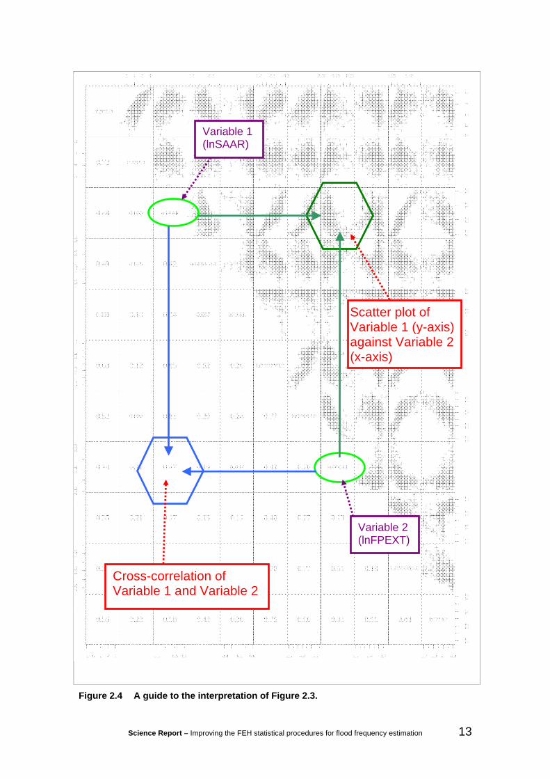
Science Report – Improving the FEH statistical procedures for flood frequency estimation 13
Figure 2.4 A guide to the interpretation of Figure 2.3.
lnQMED
2 4 6 8
++++
++++
+
++
+++
++++
++
+++
+++
++++++++
+
+++++
++++
+++
+++ +++ +
+++++
+
++++
++++
+
++
++++++
+
+++++
+ +++
+
++++++
+
+
++++
+++
++++
+++
+++
++
+++
++
++
+
++
++
++++
+
+++++
+
++
+
+
++++ +
++++++
+++
+
++
++++
++++
++
++++++
+++
+
+ ++
++++
++++++
+
++
+
+
+
+
+
++++
+++
++
++++
++
++
+++
+
++++++++++
+++
+
+
++
+++
++
++
+
+
+
++++++++++
+
+ +++
+
++
+
++++
++++
+
++
+
+
+
++++++
++
+++ +
++
++
+
++++++++
++
++
+
+
+++
+
+++
++
+++
++
+++
++ +++++++
+
+++
+
+++
++
+
+++
+
+++
++++++++++++
+++ ++
++++
+
++
++++
+
++++ +
++
++
+
++
+++
+
+++
+
++
++++
+
+++
+
+
++
+ +++
+
+
++
+
++++
++
+++
+++++
+++
+++ ++
+++
+
++++
+++
++
++
+
++
++
++
++++
++
+
+
+
+
++++
+
+++++++
++++
+++
+++++
++
++++
++
+
+
++++
+
+
++++ +
+
++++
+++++
+++
++
+++
++
++
++
++++ ++
+
+ ++++
++
+++++++
+++ ++++
++
+++
++++++++
++
++++
++
++
++ +++ ++
+
+
++
+++
++++
++++
+
+++
+++++++++
+++++++
++
+++
++ + ++ ++
+++++
+
+++ +
++++
+
++
+++ +++
+
++++ +
+++ ++
++++++
+
+
++++
++ +++++
++ +
+ ++
++
++ +
++
++
+
++
++
++++
+
+++++
+
++
+
+
+++++
++++++
++ +
+
++
++++
++++
++
+++++
+
+++
+
+++
++++++++++
+
++
+
+
+
+
+
+++++++
++
++++++
++++++
+++++++++++++
+
+
++
+++++
++
+
+
+
+++
+++++++
+
++++
+
+++
++++
++++
+
++
+
+
+
++++++++
++++
++++
+
++++++ ++
+++++
+
+++
+
++++
+
++
++++
++++ +++++
++
+
+++
+
+++
++
+
++++
++++
+ ++++++++
+ +++++ +++
++
+
++
+ ++
+
+
+++ ++
++
++
+
+++
++
+
+ ++
+
++
++++
+
+++
+
+
++
+++++
+
++
+
++
+++++
++++++
+
++
++
+++ +
++
+
+
+++
++
++
++
+++
+++
+++
+++++++
+
+
+
++
++
+
++ +
+++ +
++++
++++++++
++
+++
++
++
+
+ ++++
+
++++++
++++
++++
+++++
+
+++
++
++
++
++ ++++
+
+++
+ ++
++++++
+++++++
++++++
+
++++++++
++
+++++ +
++
−1.5 −0.5
++++++++
+
++
+++
+++++
++++
+++
+++++++++
+++++
++++
+++
+++++++
+++++
+
++++
+++++
++
++++++
+
+++ ++
+ +++
+
++++
++
+
+
++++
+++++++
+++
+++
++
+++
++
++
+
++
++
++++
+
+++++
+
++
+
+
+++ + +
+++ +++
+++
+
++
++++
++++
++
++ +
+++
+++
+
+ ++
+++
++ ++ ++
+
+
++
+
+
+
+
+
+++++ ++
++
++++
++
+++++
+
++++++ +++++++
+
+
++
+++
++
++
+
+
+
+++
++ +++ ++
+
+++ +
+
++
+
++++
++++
+
++
+
+
+
++++++++
++++
++
+ +
+
++++++++
+++++
+
++ +
+
++++
+
++
++
++
+ ++++++ +++ +
+
+++
+
++ +
++
+
++
++
++++
+++++++++++
+++++++++
+
++
++++
+
++++ +
+ +
++
+
+++
+ +
+
+++
+
++
++++
+
++ +
+
+
++
+++++
+
+++
+++++
++++
+++++
++++++ ++
++
+
+
++
+++
+ +
++
+++
++
++
+ +
+++++++
+
+
+
+++
++
+++
++++
++++
+++++
+++++
+++++
++
+
+++++
+
++ ++++
+ ++++
++ ++
++++
+
+++
++
++
+++++
+++
+
+++
+++
++ ++++
+++
+++ +++
++++
+
+++++++
+
++
+++ +
++
++
++ +++++
+
+
++
+++
++ ++++
+ ++
+++
+++++++++
++++ +
++++
+++
++++ + ++
+++++
+
++++
+++ +
+
++++++++
+
++++++++++
++++
++
+
+
++++
+++++++
+++
+++
++
+++
++
++
+
++
++
++++
+
++++
+
+
++
+
+
+++++
+ +++++
+++
+
++
++++
++++++
+++
+++
+++
+
+++
+ +++++ ++++
+
++
+
+
+
+
+
++++
+++
++
++++++
++++++
++++++ +++++++
+
+
+++++++
++
+
+
+
++++++ ++++
+
++++
+
+++
++++
++++
+
++
+
+
+
++++++++
++++
++
+ +
+
++++++++
++++
+
+
++++
+++++
+++
++++++++++++++
+
++ +
+
+++
++
+
++++
+++++++++++++++
+ +++
+++++
+
++
+++
+
+
+++++
++
++
+
+++
+ +
+
+++
+
++
++++
+
++++
+
++
+++
++
+
+++
++++++++++++++
++
++
+ +++
+++
+
++
+++++
++
+++
++
++++
+++++++
+
+
+
++
+++
+++
+ +++
+++ +
+++
+++ ++
++
+++
++++
+
++++
+
+
++++++
++++
++++
++++++
+++
++
++
++
+ ++++ +
+
+++
+++
++ ++++
+ ++++++++++++
+
++++++++
++
++++
+ +
++
−1.4 −0.8 −0.2
++ +++ ++
+
+
++
+++
++++
+++++
++
+
+ ++++++++
+++++++
++
+++
++++++++++++
+
+++ +
++++
+
++
+++ +++
+
++++ +
+++ ++
++++++
+
+
++++
++ +
++++
++ +
+++
++
++ +
++
++
+
++
++
++++
+
+++++
+
++
+
+
++ +++
+ +++++
++ +
+
++
++++
++++
++
+++++
+
+++
+
+++
+++
++++++
+
+
++
+
+
+
+
+
++++++
+
++
+++++
+
++++
++
+++++++++++++
+
+
+++++++
++
+
+
+
++++++++++
+
++++
+
+++
++++
++++
+
++
+
+
+
++++++++
++++
++++
+
++++++ ++
++
++
+
+
++++
+++++
+++++++++++++++
++
+
+++
+
+++
++
+
++++
+++
++ +++
++++++++++++++++
+
++
+ +++
+
+ ++ ++
++
++
+
+++
++
+
+ ++
+
++
++++
+
++++
+
++
+++++
+
++
+
++
+ ++++
++++++
+
++
++
+++ +
++
+
+
++
+++
++
++
+++
++++
++
+++++++
+
+
+
++
+++
+++++++
++++++
++++++++
+++++++
+
+++++
+
++++++
++++++++
++
++++
+++
++++
++
++++++
+
+++
+++
+++++++++++++
+++
+++
+
++++++++
++
++++++
++
++ +++ +++
+
++
+++
++++++++
+
++
+
++++++++
+
+++++++
++
+++
+++++++
+++++
+
+++ +
++++
+
+++++ +
++
+
++++ +
++++
+
++++
+ +
+
+
++++
+++++++
+++
+++
++
+++++
++
+
++
++
++++
+
++++
+
+
++
+
+
++ +++
++++++
++ +
+
++
++++
++++
++
+++
+++
+++
+
+++
+++
+++ +++
+
+
++
+
+
+
+
+
++++++
+
++
++++++
++
+ +++
+++++++++++++
+
+
++
+++++
+ +
+
+
+
+++
++ +++++
+
+++ +
+
++
+
++
++
++++
+
++
+
+
+
+++++++
+
++ ++
++++
+
++++++ ++
++
+++
+
++++
+++++
++
++++++
+++++++++
+
+++
+
+++
++
+
++++
+ ++
++ +++
++++++ +
+ ++++
++++
+
++
+++
+
+
+ ++ ++
++
++
+
+++
+ +
+
+ ++
+
++
++++
+
++++
+
++
+++++
+
++
+
++
+ ++++
++++++
+
++
++
++++
+++
+
++
++++ +
++
+++
++
++
++
+++++++
+
+
+
++
+++
++ +
++++
++++++++++++++
+++
++
++
+
+ ++++
+
+++++
+
++++
+++++
++++
+
+++
+++
+
++++ +
+++
+
+++
+ ++
++ ++++
+ ++++++
+++
+++
+
++ +++ +++
+++
++++ +
++
0.00 0.10 0.20
++++++++
+
++
+++
+++ +++
+++
+++
+++ +++++
+
+++++++
+ +
+++
+++
+++++++++
+
++++
+++++
++++++++
+
++ +++
+ ++++
+++ +++
+
+
++++
+++
++++
+++
+++
++
+++
+ +
++
+
++
++
++ ++
+
++++
+
+
++
+
+
++++ +
+++++ +
+++
+
++
++++
++++
++
++++ +
+
+++
+
+ ++
++++
+ +++++
+
++
+
+
+
+
+
++ ++++
+
++
++++
++
++
++++
++++++++++++ +
+
+
++
+++
++
++
+
+
+
+++
+ ++ ++ ++
+
+ +++
+
+++
++++
++++
+
++
+
+
+
++ +++++
+
++++
++++
+
++++++++
+++
++
+
++++
+++++
++
++
++++
++ +++++++
+
+++
+
+++
++
+
+++
+
+++
++++ +
+++++++
+++ ++
+ +++
+
++
+++
+
+
+++++
++
+ +
+
++
+++
+
+++
+
++
++++
+
++++
+
++
++++
+
+
+++
++++
++
+++++++
+
++++++++
+++
+
++++
+++
++
+++
++
++
++
+++ +
+++
+
+
+
+++++
+++
++++
++++++++
+++++
+
+++++++
+
+++++
+
++ ++++
++++
+++++
++++
+
+++
++
++
+++++
+++
+
+++
+++
++++++
+++
++ ++++
++
+++
+++++++
+
++
++ ++
++
++
++++
++++
+
++
+++
++++
+++++
++
+
+++++++++
+++++++
++
+++
++++++++++++
+
+++ +
++++
+
++
+++ +++
+
++++ +
+++++
+++ +++
+
+
++++
++++ +++
+++
+++
++
+++++
++
+
++
++
++++
+
+++++
+
++
+
+
+++++
++++++
+++
+
++
++++
++++++
++++++
+++
+
+++
+++
+++++++
+
++
+
+
+
+
+
+++++++
++
++++++
++++++
+++++++++++++
+
+
++
+++
++
+ +
+
+
+
+++
+++++++
+
++++
+
++
+
++++
++++
+
++
+
+
+
++++++
++
++++
++++
+
++++++++
++++
+
+
+++
+
++++
+
++
+++
++++++++++++
+
+++
+
+++
++
+
++++
++++
++++++ +++++++
+++++
++
+
++
++++
+
+++ ++
++
++
+
+++++
+
+++
+
++
++++
+
++++
+
++
+++++
+
+++
++
+ ++++
+++++++
++++++++
+++
+
+++++++
+++++
++++
++
+++++
++
+
+
+
++
+++
+++
++++
++++++++++++++
+++++++
+
+++++
+
+++++
+
+++++
+++++++++
+++
++
++
++++++++
+
+ ++
+++
+++++ ++ +
+++++
++++
+++
+ +++++++
++
++++++
++
1.25 1.40
++ +++ ++
+
+
++
+++
++++++++
+
++
+
+++++++++
+++++++
++
+++
+++ ++++
+++++
+
++++
++++
+
+++++ +++
+
++++ +
++++
+
++++++
+
+
++++
++ +++++
+++
+++
++
++ +
++
++
+
++
++
++++
+
++++
+
+
++
+
+
+++++
++++++
+++
+
++
++++
++++
++
++++++
+++
+
+++
+++
++++++
+
+
++
+
+
+
+
+
+++++++
++
++++++
++
++++
+++++++++++++
+
+
+++++++
++
+
+
+
++++++++++
+
++++
+
+++
++++
++++
+
++
+
+
+
++++++++
++++
++++
+
++++++ ++
+++++
+
+++
+
++++
+
++
+++
+++
++ +++++
++
+
+++
+
+++
++
+
++++
+ ++++ ++++++++
+ +++
++ +++
++
+
++
+++
+
+
+++ ++
++
++
+
+++
++
+
+ ++
+
++
++++
+
++++
+
++
+++++
+
++
+
++
+++
++
++++++
+
++
++
+++ +
++
+
+
+++
++
++
++
+++
++++
++
+ +++
+++
+
+
+
++
++
+
++ +
++++
++++
+++
++
+++++
+++
++
++
+
+ +++
+
+
++++++
++++
++++
+++++
+
+++
++
++
++
++ +++ +
+
+++
+ ++
++++++
++++++ +
++++
+++
++ ++++++
++++++
+ +
++
−2
02
46
++++++++
+
+ +
+++
+++++
++++
++
+
++ +++++++
++++++ +
++
+++
+++
+ ++++++++
+
++++
+++++
++
++++++
+
+++++
+++++
++++++
+
+
++++
+++++++
+++
+++
++
+++
+ +
++
+
++
++
++++
+
++++
+
+
++
+
+
+++++
++++++
+++
+
++
++++
++++++
++++++
+++
+
+++
++++
++++++
+
++
+
+
+
+
+
+++++++
++
++++++
++++++
+++++++++++++
+
+
+++++++
++
+
+
+
++++++++++
+
++++
+
+++
++++
++++
+
++
+
+
+
+++++++
+
++++
++++
+
+++++++ +
+++++
+
++ +
+
+++++
++
+++++++++++++++
+
+++
+
+++
++
+
++++
+++
+++++++++++++++++++++
+
++
+++
+
+
+++++
++
++
+
+++
++
+
+++
+
++
++++
+
++ +
+
+
++
+ +++
+
+
++
+
++
+++
++
++++++
+
++
++
+ +++
+++
+
+++
++
++
++
+++
++++
++
+++ ++
++
+
+
+
++
+++
+++
++++
++++
+++
+++ ++
++
+++++++
+
+++++
+
+++++
+
++++
++ ++
++
+++
+
+++
++++
++
++++++
+
+++
+++
+++++ ++++
++++++++
+++
++++++++
+++
+++++
++
24
68
0.72 lnAREA
+++++ ++
+++
++++
++
++
+
++
+
+
+
++
+++++++++
+++
++++
++
+++
++
+++
+
+
+++++
+
++++
+++
++
+++++++
+
+
++++
++
++ +
+
++
++++
+
+
++++++
+++++
+++
+++
++
+
++
++
++
+
++++
++++
+
+++++
+
++
+
+++++
+ +++
+++
++
+
+
+
++++
+
+
+++++
++++
+
+
++
+
+
++
++++++
++++++
+++
+
++++
++++++
++++++++
++
+++
+
+++++++++++++
+
+
++++
+++
++
++
+
+++ ++
+++++
+++++++
++
++++
+
++
+
+++
+++
+++++
+++
+++
+
++++
+
++++++ +
+
+
++
+
++
++
+
+
++++
+++ +
++
+++
+++
++++++
+
+++
+
++
+
++
+
+
+++
+++
+
++
+++++
+++ ++++
+ +++
++
+
++
++
++ ++++
+
+
++
++
++++++
++
++
+
++
++++
+
+ ++
+
+
++
++ +++
+
++
+
+++++
+
+++
++++
+
+ +++
++
++
+++
+
+
++++
++
+
+
+++ ++
+
++++++++
++
+
+
+
++ +++
+
++
+++
+++
++ ++
++++
+++
+
+++
++
++
+
++++
+
+
+++
+++
++++
++
+++
++++
+
+++
+ ++
+
+
+
++
++
++
+
++++
++ ++
++++
+++
+++
+++++++
+++++
++++
++
+++++
+
++
+++++++
++++
+++
+++++
+++
+
+
++
+++++++++
+++
++++
++
+++
++
+++
+
+
+ ++++
+
++++
+++
++
++++++++
+
+++ +
++
+++
+
++
++++
+
+
+++++++++++
+++
+++
++
+
++
++
++
+
++++
++++
+
+++++
+
++
+
+++
++
++++
+++
+++
+
+
++++
+
+
+++++
++
++
+
+
++
+
+
++
++++ ++
++ ++ ++
+++
+
++
++
++++ +
+
+ +++ +++
+
++
+++
+
+++
+++ +++++++
+
+
+++ +
+++++
++
+
+++++ +++ +
+
++
++ + ++
++
++++
+
++
+
+++
+++
+++++
+++
++
+
+
+++ +
+
+++++
+++
+
++
+
++
++
+
+
++++
++
+ +
++
++ +
+++
++ +++ +
+
+++
+
++
+
++
+
+
+++
+++
+
+++++
++++++
+++
+++++
+
+
++
++
+++++ +
+
+
++
+++++++ +
++
++
+
++
++++
+
++++
+
++
+++++
+
++
+
+++++
+
+++
+++++
++++++
++
+++
+
+
++ ++
++
+
+
+++++
+
++
++++++
++
+
+
+
+++ ++
+
++
+++
+++
++++
+++
++++
+
++
+++
++
+
++++
+
+
+++
+++
+ ++++
++ ++++++
+
+++
+++
+
+
+
++
++
++
+
++++
++++
++++++
+
+++
+++++++
++
+++++
++
++
+++ +
++
++
++++++++
+++++
+
++
++
+
++
+
+
+
++
+++++++++
+++
+ +++++
+++
++
++ +
+
+
+ ++ ++
+
++++
+++++
+ ++++++
+
+
++++
++
+++
+
++
++++
+
+
+++++ ++++++
++++++
++
+
++
++
++
+
++++
++++
+
+++++
+
++
+
++++
+++ +
++++
++
+
+
+
++++
+
+
+++++
+++
+
+
+
++
+
+
++
++ +++++ +++++
+++
+
++
++
+++++
+
++++++++
++
+++
+
++++++ +++++++
+
+
+++++++++
++
+
++++++ +++
+
+++++++++++++
+
++
+
+++
+++
+++++
+++
+++
+
+++ +
+
++++++++
+
++
+
++
+++
+
++++++
++
++
+++
+++
++++ ++
+
++ +
+
+++
++
+
+
+++
+++
+
+++++++++++
+ ++
++++++
+
++
++++++++
+
+
++
+++++++ +
++
++
+
++++++
+
++++
+
++
+++ +
+
+
++
+
+++++
+
+++
+++++
++++
+ +
++++++
+
++ ++
++
+
+
+++++
+
++
++++++
++
+
+
+
+++ ++
+
++
++++
+++
+++
++
++
++ +
+
++
++
+
++
+
++ ++
+
+
+++
+++
++++
++
+++++++
+
+++
+++
+
+
+
++++
++
+
+++ +
+++
+++++
+ ++
++++++++++
+++++++++
++
+ +++
++
++
+++++ ++
+++
+++
+
++
++
+
+++
+
+
++
+ ++++
++++
+++
++++
++
+++
++
+++
+
+
+++++
+
++++
+++
++
++++++++
+
++++
++
++ +
+
++
++++
+
+
+++++++++++
++++++
++
+
++
++
++
+
++++
++++
+
+++++
+
++
+
+++
+++ + +
++++
++
+
+
+
+++++
+
+++++
++
++
+
+
++
+
+
++
++++++
++++++
+++
+
++
+++++
+++
+++++++
+
++
+++
+
+++
++++++++++
+
+
++++++
+++
++
+
++++++++++
+++++++++++++
+
++
+
+++
+++
+++++
+++
+++
+
++++
+
++++++ +
+
+
++
+
++
+++
+
++++++++
++
+++
+++++++++
+
+++
+
+++
++
+
+
+++
+++
+
++
++++++++++++
++++++
+
++
++
++ ++ ++
+
+
++
++
++++++
++
++
+
++
++++
+
+++
+
+
++
+++++
+
++
+
++++
+
+
+++
+++++
++++
++
++
+ ++
+
+
+ +++
++
+
+
+++ ++
+
+++
+++++
++
+
+
+
+++++
+
++
++++++++++
++++++++
+++++
++
+
++++
+
+
+++
+++
++++++
++++
+++
+
+++
++++
+
+
++
++
++
+
++
+++
+ +++++++++
+++++++
++++
++++
++++
++
++++++
++
+++++ +++
+++
+++
+++++
++
+
+
+
++
+++++
++++
+++
++++
++
+++
+++++
+
+
+++++
+
++++
+++
++
+++++
+++
+
++++
++
+++
+
++
+++ +
+
+
+++++++++++
+++
+++
++
+
++
++
++
+
++++
++++
+
+++++
+
++
+
++++
++++
+++
+
++
+
+
+
++++
+
+
+++++
++
++
+
+
++
+
+
++
+++++ +
+ ++++ +
+ ++
+
++
+++++
+++
++++++++
++
+ ++
+
+++++++++++++
+
+
+++ +
++++ +
++
+
+++ ++
+++++
++
++ ++++
++ +++
+
++
+
+++
+++
+++++
+++
++
+
+
++++
+
++++++ ++
+
++
+
++
++
+
+
++++++
+ +
++
+++
+++++++++
+
+++
+
+++
++
+
+
+++
+++
+
+++
++++
+++ ++ ++
++++
++
+
++
++++ +
+ ++
+
+
++
++
++++++
++
++
+
++
+++
+
+
+ +++
+
++
+++++
+
++
+
++++
+
+
+++
++++
+
++++
++
++
++++
+
++++
++
+
+
+++ ++
+
+++
+++++
++
+
+
+
++ +++
+
++
++++
++++++
++++
++++
++
+++
++
+
++++
+
+
+++
++
+
++++
++
+++++++
+
+++
+++
+
+
+
++
++
++
+
++++
++ +
++++
++ ++
+++
++++
++++++ ++
+ +++
++++++
++
++
+++++++++++
+++
++
+++
+++
+
+
++
+++ +++++
+
+++
++++
++
+++
++
+++
+
+
+++++
+
++++
+++++
++++++++
+
++ ++
++
+++
+
++
+ +++
+
+
+++++++++++
++++++
++
+
++
++
++
+
++
++
++ ++
+
+++++
+
++
+
+++++
++++++
+
++
+
+
+
++++
+
+
+++ ++
++
++
+
+
++
+
+
++
++++++
++++++
+++
+
++
++
+ +++++
++++ ++++
++
+++
+
+++
+++++++++ +
+
+
++++
+ ++++
++
+
++++ +
+ ++ ++
++
+++
+ +++
++++
+
++
+
+++
++ +
++ +++
+++
++
+
+
++++
+
+++++
+++
+
++
+
++
++
+
+
+++++
+++
++
+++
++++
+++++
+
+++
+
++
+
++
+
+
+++
+++
+
+++
++++++ ++
+++
+++ ++
+
+
++
++
+ ++++ +
+
+
++
++
+ +++++
++
++
+
++++
++
+
+++
+
+
++
++++
+
+
++
+
++++
+
+
+++
++++
+
++++++
++++++
+
+++
+
++
+
+
++++ +
+
+++
++ + ++
++
+
+
+
+++++
+
++
+++
+++
++++
++
+++++
+
+++++
++
+
++++
+
+
+++
++
+
++++
+++++
++++
+
+++
+ +++
+
+
++
++
++
+
+++ +
+++
++++
++++
+++
++++
++++++++++
++
++
++++
++
++
+++ ++++++
++
+ ++
++
++
+
+++
+
+
++
+++++
++++
+++
++++
++
+++
+++++
+
+
+++++
+
++++
+++
++
+ ++++++
+
+
++++
++
+++
+
++
+ +++
+
+
++++++++ +++
++++++
++
+
++
++
++
+
++++
++++
+
+++++
+
++
+
++++++++
++++
+++
+
+
+++++
+
+++++
++++
+
+
++
+
+
++
++++++++++++
+++
+
+++
+++++++
++++++++
++
+++
+
+++++++++++++
+
+
+++++ +++ +
++
+
+++++++++
+
++++++++
+++++
+
++
+
+++
+++
+++++
+++
+++
+
++++
+
++++++++
+
++
+
++
+++
+
+++
++
++ +
++
+++
+++++++++
+
+++
+
+++
++
+
+
+++
+++
+
+++++
+ ++
++++++
++++
++
+
++
++++++++
+
+
++
++
++++++
++
++
+
++
++++
+
++++
+
++
+++++
+
++
+
++++
+
+
+++
+++++
++++++
++++++
+
++++
++
+
+
+++++
+
++
++++++
++
+
+
+
+ ++++
+
++
+++
+++++++
++++++++
+++++
++
+
++++
+
+
+++
++
+
+++++
++++++++
+
+++
++++
+
+
++
++
++
+
++++
++ +++++
++ +
+
++++++
++++
++
+++++++
++
++++++
++
+++++ ++
++
++
+++
+++
++
++
+
+
+
++
+++++++++
+++
++++
++
+++
+++
++
+
+
+++++
+
++++
+++
++
+++++++
+
+
++++
++
+++
+
++
++++
+
+
++++++
+++++
+++
+++
++
+
++
++
++
+
++++
++++
+
+++++
+
++
+
+++++
++++
+++
++
+
+
+
++++
+
+
+++++
++++
+
+
++
+
+
++
+++++ +++++++
+++
+
++++++++++
++++++++
++
+++
+
+++++++++++++
+
+
+++++++
++
++
+
++++++++++
+++++++
++
++++
+
++
+
+++
+++
+++++
+++
+++
+
++++
+
+++++
+ ++
+
++
+
++
++
+
+
++++
++
+ +
++
+++
+++
++++++
+
+++
+
++
+
++
+
+
+++
+++
+
++
++++++
++ ++++
+ +++
++
+
++
++
++ ++++
+
+
++
++
++++++
++
++
+
++
++++
+
+ ++
+
+
++
++ +++
+
++
+
+++++
+
+++
++++
+
++++
++
++
+++
+
+
++++
++
+
+
+++++
+
++++ +++
+
++
+
+
+
++ +++
+
++
+++
+++
++ ++
++
++
+++
+
+++
++
++
+
++++
+
+
+++
++
+
++++
++
+++
++++
+
+++
+ ++
+
+
+
++
++
++
+
++
+++
+ ++++++
+++
+++
+++++++++
+ ++++++
+++++++
+
++
++++++++
++
+++
+
+++++
+++
+
+
++
+++++
++++
+++
+++ +
++
+++
+++
+ +
+
+
+++++
+
++++
+++++
++++++++
+
++++
++
+++
+
++
++++
+
+
++++ ++
+ ++++
+++
++ +
++
+
++
++
++
+
++++
++++
+
+++++
+
++
+
+++++++++
+++
++
+
+
+
++++
+
+
+++++
++++
+
+
++
+
+
++
++++++++++++
+++
+
++++++++++
++++++++
++
+++
+
+++++++++++++
+
+
++++
+++++
++
+
++++++++++
+++++++++++++
+
++
+
+++
+++
+++++
+++
+++
+
++++
+
++++++++
+
++
+
++
++
+
+
++++++++
++
+++
+++
++++++
+
+++
+
++
+
++
+
+
+++
+++
+
++++++++++++++
++++++
+
++
+++ ++
+++
+
+
++
++
+ +++++
++
++
+
++++++
+
+++
+
+
++
++++
+
+
++
+
++ ++
+
+
+ ++
++++
+
++ ++
+ +
++++
++
+
+++
+
++
+
+
++++ +
+
++++++ +
+
++
+
+
+
+ ++++
+
++
+++
+++++++
++++
++ +
+
+++++
++
+
++++
+
+
+++
++
+
++++
++
+++++++
+
+++
++++
+
+
++
++
++
+
++
+ ++
++++++
++++
++++++
+++++
++++++++
+++++++
+
++
0.48 0.053 lnSAAR ++
++
+
+++
+++
+++
+++++
++
+++++++
+++++++
+++++
++
++
++
+
++
+
+
++
++
++++++++
+
+++
++
++
+++
+++
+++++
++
++
+
+++
+++++++
+++
++
+
++++++
+
++
+++
+
+
++
+
+++
++++
++++
++
++++
++
+
+
+
+++
++
+++
++++
+
++
+ + +++++
+++++++ +++ +++ +++ ++ +++ ++ ++ ++ ++++ +++ ++
+++++ +++ +
++ ++++++++++++++++ ++++++++++++
++++
+++
+++++
++
+++ ++ ++++ + +
+ ++ +++++++ +++
++ ++ ++++++ +++++++++
++++
+++++
++++++
+++
+++
+++
+ ++
++ +++
+++
+
++
+++
+++++
++
+
+++
+
++++++++
+
++
+++++++
++++
+
+++++
++++
+
++
+
++ +
+
++
+++
+
++++ +
+
+
++++
+
++++++
+
+
+++
++
+
++++ ++++++++++
+++++
+++
++
+
++
++
+++
+
+ ++
++
+++
+
+
++
++++
+ ++
+++++++
+
+
++
++++
+
++
+++++
++++
++++++
+
+
+
++
++++
+
+
+
++++++ +++++ ++++
++ ++++++
+
++++
+
+
+
+++
+
+++
+++++
++
+
+
+++++
++ ++++
++++++
++++++
++++ +++++ ++
+
++
++
++
+
++ +
+ +++
+++
++
++++
++
+++++++++++++++++++++
++
+
++
+
+
++
++
++ ++++++
+
+++
++
+++++
+++
+++
++
++
++
+
+++
++++++++++
+ +
+
++++++
+
++
+++
+
+
++
+
+++
++++
++++++
++++
++
+
+
+
+++
++
+ ++
++++
+
++++ +++
+ +
++++++++++++++++++++++++ +++++
++++++ ++
++++++++++++++++++++++++++ +++++++
+++++++++++
++ +++
+++
+ ++++++++++++++++++++++++++++++++++++++++++++++
+++++
++++++++++++++++++
++++++++
+
+++++++++ +++
+
+++
+
++++++++
+
++
+++++++
++ ++
+
+ +++++
+++
+
++
+
+++
+
++
+++
+
++++ +
+
+
++++
+
++++++
+
+
++
+++
+
+ ++++++++++++++
+++++ +
++
+
+
+ +
+++++
+
+++
++
++
+
+
+
++
+++
+
+++
++++++++
+
++
++++
+
++
+++
++
+ +++
+++
++
+
+
+
+
++
+++++
+
+
+++++++++++++++
++++++++
+
++++
+
+
+
++
+
+
+++ +++
++
++
+
+
+++++
++++++++++++++++++++++++
+ ++++
+
++
++
++
+
+++
+++
+++
++
++
+++
++
++++ ++++ ++++
++++++
+++
++
+
++
+
+
++
++
++++
++++
+
+++
++
++
+++
+++
++ ++
+
++
++
+
+++
+++++++++
+
++
+
++++++
+
++
+++
+
+
++
+
+++
++++
+++++
+
++++
++
+
+
+
+++
++
+ ++
++++
+
++
+++++
++
++++++++++ ++++++++++++++++++
++++++++
++++++++++++++++++++++++++++++++++
++++++++++++++++++++++++++++++++++++++++++++++++++++++++++++++++
++
+++++
+++ +++
++++++++++++
++++++++
+
++++++++++++
+
+++
+
++++++++
+
++
+++++++
++++
+
+++++++
+++
++
+
+ ++
+
++
+++
+
+++++
+
+
+++
+
+
+++++ +
+
+
+++++
+
++++++++++ ++++
+++++
++++
+
+
++
++
+ ++
+
++ +
++
++
+
+
+
++
++++
+++++
+++++
+
+
++
++++
+
++
+++++
++++
++++++
+
+
+
++
+++++
+
+
++++++++++++++++
+++++++
+
++++
+
+
+
++
+
+
++++++++
++
+
+
++++++++++
+++++++
++++++
+++++++++++
+
++
++
++
+
+++
+++
+++
+++++++
+++++++
+++ ++++++++
++
+++
++
+
+++
+
++
++
++++
++++
+
+++
++
++++
+
+++
++++
+
++
++
+
+++
+++
+++++++
++
+
++
++++
+
++
+++
+
+
++
+
+++
++++
++++
++
++++
+ +
+
+
+
+++
++
+++
++++
+
++
+ ++++++
+++++ ++++++ ++++ +++++++ ++ ++++ +
+ +++++ +++++++
++++++++++++ ++++ ++++++++++++
+ ++++
+++++ ++
+++++
++
+++++ ++++ +++++++++++++++++++++++
++++++ +++++++++
+++++
++++++
++++
++
++++++
++++++
++
+
++
++++++++
++
+
+++
+
++++++++
+
++
++++++
+
++ ++
+
+++ ++
++++
+
++
+
+ ++
+
++
+++
+
++++ +
+
+
++++
+
++++++
+
+
++++
+
+
++++ ++++++ ++++
+++++
++++
+
+
++
++
+++
+
+ ++
++
++
+
+
+
++
+++
+
+++++
++++++
+
++
++++
+
++
+++
++
++++
++++
++
+
+
+
++
+++++
+
+
++++ ++++++++++++
+++++++
+
++++
+
+
+
+++
+
++++++
++
++
+
+
++++++
+++++
++++++++
++ +++ ++++++++++
+
++
++
++
+
+++
+++
+++
++
+++++
++
++++++ ++++++++++++++ +
++
+
++
+
+
++
++
++++
++++
+
+++
++
+++++
+++
+++ +
+
++
++
+
+++
+ ++
+++++++
++
+
++++++
+
++
+++
+
+
++
+
+++
++++
++++
++
++++
++
+
+
+
++++
+
+++++ +
+
+
++
+++++
++
+++++++++
+++++++ + +++++
+ ++++++++ +++++
++ ++++ +++
++ ++++++ ++++ ++++++++++++ +++ +++
++ ++
+++++ ++
++
++ ++ +
+++ ++++++++
++++++++++ ++ +++
+++++
+ +++++++++++
+++++
++++++
+++
+++++
+++ +
++++++
++
+
++++
++++++++
+
+++
+
++++++++
+
++
++++++
+
++++
+
+++++ +
++ +
+
++
+
++ +
+
++
++ +
+
+++++
+
+
+++
+
+
++++++
+
+
+++++
+
+++++ ++++++
+ ++++++++++++
+
++
+++++
+
+++
++
++
+
+
+
++
++ +
+
+++
+ ++
++++
+
+
++
++++
+
++
+++
++
++++
+++
+++
+
+
+
++
+++++
+
+
++++++ ++++++++++++++ +++
+
++++
+
+
+
+++
+
+++++ +++
+++
+
+++++
++ +++
++++ +++
+++++++++++ +++ +++
+
++
++
+ +
+
+++
+++
+++
++
++
+++
++
++++++++ ++++
++++++
+++
++
+
+++
+
++
++
++++++++
+
+++
++
++
+++
+++
++ +++
++
++
+
+++
+ +++++++
++
++
+
++
++++
+
++
+++
+
+
++
+
+++
++++
++++
++
++++
++
+
+
+
+++
++
+++
++++
+
+++++
++++
+++++++++
+++++++++++++++++++++++++++++++++++++++++++++++++++++++++++++
+++++++ +++ +
++ ++++
+++++
++++++++++++++++++++++++++++++++
++++++++++++
+++++
++++++
+++
+++
+++
+++
++++++
++
+
++++++++++
++
+
+++
+
++++++
++
+
++
+++ ++++
++++
+
++++++++++
++
+
+++
+
++
+++
+
+++++
+
+
++++
+
++++++
+
+
+++++
+
++++++++++ ++++
++ +++
+++
++
+
++
+++++
+
+++
++
+++
+
+
++
++++
+++++++++++
+
+ +
++++
+
++
+++
++
++++
++++++
+
+
+
++
+++++
+
+
++++++++++++
++++
+++++++
+
++++
+
+
+
+++
+
+++
+ ++++
++
+
+
++++ +
+++ ++
++++ +++
+++ ++++++++ +
+++++
+
++
++
++
+
+++
+++
++++++
++++
+++++++++++
+++++++
+++
++
++
+
+++
+
++
++
++++
++++
+
+++
++
+++++
+++
++++
+
++
++
+
+++
+++++ ++++
+
++
+
++++++
+
++
+++
+
+
++
+
+++
++++
+++++
+
++++
++
+
+
+
++++
+
+++
++++
+
++
++++++ +
+++++ +++++++++++++++++ +++++++
++++++++++++++++++++++++++++++++++++++++++++++++++
+++++++
+++++++
+++++++++++++++++++++++++++++++++++++++++
++
+++++
++++++
+++
++
+++
++++
+++++
+++
+
+++++
++++++
+
+
+++
+
++++++
++
+
++
++++++
+
++++
+
++++++
++++
++
+
+++
+
++
+++
+
+++++
+
+
+++
+
+
++++++
+
+
++
++
+
+
++++++++++++++
+++++
+++
++
+
++
++
+++
+
+++
++
++
+
+
+
++
++++
+++
+++
++++
+
+
++
++++
+
++
+++
++
++++
++++
++
+
+
+
++
++++
+
+
+
+++++++
+++++++++
+++++++
+
++++
+
+
+
++
+
+
+++
+++++
++
+
+
+++++
+++++
+++++++
++++ +++++++++++++
+
++
−0.
50.
00.
51.
0
++
++
+
++ +
+++
+++
+++++
++
+++ + +++
++++++ +++
++++
+++
++
+
+++
+
++
+ +
++++++++
+
+++
++
++
+++
+++
+++++
++
++
+
+++
+++
+++++++
++
+
++++++
+
++
+++
+
+
++
+
+++
++++
++++++
++++
++
+
+
+
+++++
+++
++++
+
++
+++++++
++++++++++++++++++++++++++++++++++++++++++++++++++++++++++++++++++++++++++++++
+++++++++++
+++++++++++++++++++++++++++++++++++
++++++++++++
+++++
+++++++
+++++++++++
++++++++
+
++++
++++++++
+
+++
+
++++++++
+
++
+++++++
++++
+
+++++++++
+
++
+
+++
+
++
+++
+
+++++
+
+
+++
+
+
++++++
+
+
++++
+
+
++++ +++++ ++++++
++++++
++
+
+
+ +
++++
+
+
+++
++
+++
+
+
++
++++
++++++
++++
+
+
+ +
++++
+
++
+++
++
++++
++++
++
+
+
+
++
++++
+
+
+
++++++++++++++ ++
+++++++
+
++++
+
+
+
++
+
+
+++
+++++
++
+
+
++++ +++++++++++++++
++++++++
+++++++
+
++
−1.
5−
1.0
−0.
50.
0
0.49 0.029 0.42 lnBFIHOST
+++
++++ ++ ++
++
+
++ +++++ ++ +
++++++++++++++++++++
+++
++
+++
++
+
++ ++++++
+++
+ +++ ++++
++
++++++
++++
+ ++
+
++++
+++++++ +
+++++++++++++
+
+
++
+
+++
+
+++
+++++
+
++++
++
++
+
+
++
+
+
+ ++
++++
+++
+
+
+
+++ +
+++
++++
++
+
+
++
+
++
++
++
+
+
+
+
+
++
++
+
+
+++
+
+
+
++++
++
+
+
++
+++++++++++++++
+
+++++++
+++++++
++
++
++ +++
+
+++ ++
+
+
+
+++
+
+
+
++
++++++
+
+++++
+
+
+++++
+
++++++
++
+++
++++++++++++++
++
+++++++
+
++
+
+++
+
+++++
++
++
+++ +++
+
++++
++++++++
+++++++++++
+++++ +++++
++
++++
+
++
+
+
++
++++
+++
++++
+++++++++++
+
+++++++
+ +++
++++++++++++++++ ++++ +
++
++
+
++++
++
++
+
++
+
++++
+++
++
+++++++++
++
++
++++
++++
+++
+++
+
++++ ++
+
+
+++
++
+
+
+
++ ++++++
++++
+++++++
+++++++
++++++
+ +++ ++++ +++++
++
++
+
++++
+
+++++++++++++++
+++
+++++
+ ++++
++
+
+++++ +++
+++++
+
+++++++
++++++++
++ +++++++++
++++
++ +
++
+++++
+
+++++ +++
+++
+++ ++++
+
+++
++++
+
++++
+++
+
++++++++++
+++
++++++ +
+++++
+
+
++
+
+++
+
+++
+++++
+
++++
++
++
+
+
++
+
+
+ ++
++++
++
+
+
+
+
++ ++
+++
++++
++
+
+
++
+
++
++
++
+
+
+
+
+
++
++
+
+
+++
+
+
+
++
++
+++
+
++
+++
++++++++++++
+
+++++++
+++++++
++
++
+++++
+
+++++
+
+
+
+++
+
+
+
++
++++++
+
+++++
+
+
+++++
+
++++++++
+++
++++++ ++++ ++++
++
+++++++
+
+++
+++
+
+++++
++
++++++++
+
++++
++++++++
++++
+++++++++++++++++++
++
++
+
+++
+
++
+++ ++++
++ ++
++++ ++++++ +
+
+ ++++++
++++
+++++
+++++
+++++++++++
++
++
+
++++
++
++
+
++
+
++++
+++
++
+++++++++++
++++++++++
+++++++
+++++++
+
+++++
+
+
+
++++++++
++++++++++
+
++++++
+
+++++++++ ++
++++++++
++
++
+
+++++
+++++++
++++++
++
+++++
+++
+++++
+++
+++
++ +++
+++++
+
+++++++++++++++
++ ++++ +++++
++++
+++
++++++
+
+
+++++ +++
++++++++
+++
++
+++
+++
++++
++ +
+
+++
++++++++++
+++++++++
+++
+
+
++
+
+++
+
+++
++++
+
+
++++
++
++
+
+
++
+
+
+++
++++
++
+
+
+
+
++++
+++
++++
++
+
+
++
+
+ +
++
++
+
+
+
+
+
++
+ +
+
+
+++
+
+
+
++
++
+++
+
++
+++++++ ++++++++
+
++++++
+
++
+++
++
++
++
+++
++
+
+++++
+
+
+
+++
+
+
+
++
+ +++++
+
++++
+
+
+
+++++
+
++++ ++
++
+++
++++++ ++++++++
++
+++
++++
+
++
+
+++
+
+++++
++
+++
+++++
+
+++
+
+++++
+++
+++
++
+++++ ++
++++++ ++
+++
++++
+
++
+
+
++
+++ +
+++
++ +
+
+++++++++++
+
+++++++
++++
++++++
+++++++++
+++++++
+
++
+
+++
+
++
++
+
++
+
++++
++
+
++
++++ ++++ +++
+++++
+++
++
+ ++
+++
+
+++++++
+
+++
++
+
+
+
+ ++++++
+
+++++
+++++
+
+++++++
+++++++++++
++++++++
++
++
+
+++++
+++++
++++++
++++
+++
++++
++++++
+++
+++++++++++
++
+
+++ +++++++
+++++ +++++++++++
+++ +
+++
++
+++
++
+
++++ ++++
+++
++++++++
++
+++
+ ++
++++
+++
+
+++
+++++++
++++++++++
+++++
+
+
++
+
+++
+
+++
++++
+
+
++++
++
+++
+
++
+
+
+++
++ ++
++
+
+
+
+
++++
++
+
+++
+
++
+
+
++
+
++
++
++
+
+
+
+
+
++
++
+
+
+++
+
+
+
++++
++
+
+
++
+++++
+ ++++ +++++
+
+++++++
++
+++
++
++
++
+++ ++
+
+ ++ ++
+
+
+
+++
+
+
+
++
++++++
+
++++
+
+
+
++ +++
+
++++
++++
+++
+++
+++++++++++
++
+++++
++
+
++
+
+++
+
++ +++
++
++++++++
+
+++
+
+++++
+++
+++
++
++++ +++
++ +++ +++
+++
++
+ +
+
++
+
+
++
++++
+++
+++
+
+++++++++ ++
+
+++++++
++++
+ +++++++ +++++++++++++++
++
+
+++
+
++
++
+
++
+
+ +++
++
+
++
+++ ++++
++++
+++++
+++++
+++
++++
+++++++
+
+++++
+
+
+
++++++
++
+++++
++++++
+++ ++++
++++ ++++++++++++ +++
+++
++
+++++
++++ +
+++ +++
++++
+++
++++
+++ +
++
++
+
+++
++++++++
+ +
+
++++++++++
+++++
++ ++++ +++++
++++
+++
+++++++
+
++++++++
+++
++++ ++++
+++++
+++
++++
+++
+
+++
+++++++++
++ +++++++++++
+
+
+++
+++
+
+++
++++
+
+
++++
++
++
+
+
++
+
+
++ +
++++
+++
+
+
+
++++
+++
++++
++
+
+
++
+
++
++
++
+
+
+
+
+
++
++
+
+
+++
+
+
+
++
++
+++
+
++
+++++++++++++++
+
++++++
+
+++++++
++
++
++ +++
+
++++
+
+
+
+
+++
+
+
+
++
++++++
+
+++++
+
+
+++++
+
++++++++
+++
+++++++++
++++ +
++
+++
+++
+
+
++
+
+++
+
+++++
++
++++++++
+
++++
++++++++
++++++ +++++
++++++++++++
++++
+
+++
+
++
+++++++
++++
+++++++++++
+
+++++++
++++
+++++
+++++
++ +++++++++++
++
+
+++
+
++
++
+
++
+
++++
+++
++
+++++++
++++
+++++
+++++
+++++++
+++++++
+
+++++
+
+
+
++++++
++
++++
+++
++++
+++++++
++++++++++++ +++ ++ ++
++
++
+
+++ ++
++ +++
+++ ++++++
+++
+++++
++++++
++
+
+++++ +
+++++++
+
+++++++
+++++++++
++++++++++
++++
++ +
+++ ++
++
+
++++++++
++++++++
+++
++
+++
+++
++++
+++
+
+++++ +++++
+++
+++++++
++
+++
+
+
++
+
+++
+
+++
+++++
+
++++
++
++
+
+
++
+
+
+++
++++
++
+
+
+
+
+++ +
+++
++++
++
+
+
++
+
++
++
++
+
+
+
+
+
++
++
+
+
+++
+
+
+
++++
+++
+
++
+++++++++++++++
+
+++++++
+++++++
++
++
+++
++
+
+++++
+
+
+
+++
+
+
+
++
++++++
+
+++++
+
+
+++++
+
++++++++
+++
++++++ +++
++++ +
++
++
+++
++
+
+++
+++
+
++ +++
++
+++++++
+
+
+++
+
+++++
+++
++++
++++++ +
++++ ++++
++
++
++
++
+
++
+
+
++
+++ +
+++
++ +
+
++++ +++++++
+
+ ++ +
+++
++++
+++++++++++++++++++++
++
++
+
+ ++
+
++
++
+
++
+
++++
+++
+++ +++ ++++ +
+ +
+++++
+++
++
+ ++
++ +
+
+++++++
+
+++
++
+
+
+
+ ++++++
+
++++
+++++ ++
++++++
+
++++ ++
++++++++ +++++
++
++
+
++++ +
+++++++++++
+++
+++
++++
+++++++
+++
++++++
+ +++ +
++
+
++++++++++
+ +++ +
+++++ ++++++
+ +++
+++
++++++
+
+
++++++++
++++++++
+++
+++++++
+
++++
+++
+
+++
+++++++++
+++++++
++
++++
+
+
++
+
+++
+
+++
+++++
+
++++
++
+++
+
++
+
+
+++
++++
++
+
+
+
+
++++
+++
++++
++
+
+
++
+
++
++
++
+
+
+
+
+
++
++
+
+
+++
+
+
+
++++
+++
+
++
+++++++++++++++
+
+++++++
+++++++
++
+++++++
+
+++++
+
+
+
+++
+
+
+
++
++++++
+
+++++
+
+
+++++
+
++++++++
+++
+++++++ ++
+++++
++
+++++++
+
+++
+++
+
+++++
++
++++++++
+
+++
+
+++++
+++
+++
++++++++++++++++++++
+++ +
+
++
+
+
++
+++++++
+++
+
+++++++++++
+
++++++ +
++++
++++++
+++++++++++++ + +
++
++
+
++++
++
++
+
++
+
+ +++
+++
++++
+ ++++++++
++
++++
++++
+++
+++
+
++++ +++
+
+++++
+
+
+
++++++++
++++
++++ ++
+
++++++
+
+++++++++++
+ +++++++
++
++
+
+++ ++
+++++++++++++
++
++++++
+++++++
+++
0.093 0.10 0.34 0.097 lnFARL++
+++ +
+
+
+
+++++
++++
+++
++
++++ ++++ +++++++
+
+++++
++ +
++
+
+
+
+
+
+
+
+
+++ +++ ++++
+++
++++ ++
+
++ ++
+ ++++
+
+++++++++++++
++ +++++++ ++++++
++ +
++
+++
++++++++++ ++++++ ++
+
++ ++++
++
+++ +++++
+
++++
++++
++++++
+ ++++++++
++++++
+++++ ++++++
+++++++
++++++++++++++++++++
+
+++++++++++++++++
+
+
+++++++
+++++++++++++++++++++++++++++++++++++++++
+
+
++ +++++++
+++ +++++++++++++++++++++++++++
+
++++++++++++++++++++++ ++++++
++++++++
+
++++++
++ +++ ++ ++
++++++ +++++
+ ++ +++
+ ++++++ +++ ++++++
+
+++++++++ +++++++++
+
+++
+
+
+
++ ++ +++++
+
++ +++
++++ ++++ +
+
++++++++++++
+
++
+
++
+
+++
++
+
+++
++++
+
++
+
+
++
++++++
+
++++++++++++++++
++++++++++++++
+
++
+
+++
+
++
+
++
+
+
++
+
++++
+
+++++++++++++
+++
++++++++++++++
+++
+++ +
+
+
+
+++++
+++++++
++++++++++ ++++ +++
+
+++++
+++
+++
+
+
+
+
+
+
+
+++ +++ ++++
+++
++++ ++
+
++++
+ ++++
+
+ +++++ +++++++
++++++++++++++++++
++
+++++++++++ +++++++ + ++
+
++ ++++++
++++++++
+
+++++
+++++
++++++
++++ +++
++++ +
+++++ ++ ++
+++
+++++++
++++++++++++ ++++ ++++
+
++++++++ ++++ +++++
+
+
++
+++ ++
++
+++ +++
+++
++++ +++++++++++++++++++++
++ ++++
+
+++++++++
++++++++++++++++++ +
+++++++++++
+
+++
+++++++++ ++++++ ++++ ++++++
++++++++
+
++ +++++++++ ++ +
+++++++ +
++++
+ ++ +++++++++++++++++++
+
+++ ++++++ +++++++++
+
+++
+
+
+
++++++++ +
+
+++ ++++++ +
++ + +
+
++++++++ +++
+
+
++
+
++
+
+++
++
+
+++
++++
+
++
+
+
++
+++++ +
+
+++
+ ++++++++++++
+++++++++++++
+
+
++
+
+ ++
+
++
+
++
+
+
++
+
++++
+
+++++++++++++++
+++ +++++
++
+++
++
+++
++++
+
+
+
+++++
+++
+++
+
++
++++++ +++++++++
+
++++ +
+++
++
+
+
+
+
+
+
+
+
++ +++++ +++++
+++++++
+
+++++++ ++
+
+++ + ++++
+++++
++++++++++++++++ ++
++
+++
+ +++++ +++ +++++ ++++
+
++++ ++
++++ ++ ++++
+
++++
++++
++++++
+++++++ + +
+++++
++++++ ++ ++++
++
+ +++++
++++ ++++++ ++++ +++++
+
++++++ +++ ++ +++ ++
+
+
+
++
++ ++ +
++
+++++ ++
++
++++++
++++++++ ++ +++ ++++++
++++++
+
++++ +++++
++++++++++++++++++++++++++
++++
+
++++
++++ +++++++++++++ +++ ++++
++ ++ +
++ +
+
+ +++ ++
+ +++ ++ +++
+++++ +++++
+
++ ++++
++++++ ++++++++++
+
++++ +++++++ +++++++
+
++++
+
+
+++++++++
+
++++++ + +++
++++
+
++ ++
+++++ +++
+
++
+
++
+
+++
++
+
+++
++
++
+
++
+
+
++
++++++
+
++++++ ++++++++++++++ +++++++++
+
+
++
+
+++
+
++
+
++
+
+
++
+
++++
+
+ +++ ++++ +++++++
++++++ + +
++
+++
+ +
+++
++++
+
+
+
+++++
+++
++++
++
++++++++ ++++ +++
+
+++++
+++
+++
+
+
+
+
+
+
+
++++++ ++++++
+++++ ++
+
++ ++
+ ++++
+
++++ +++++++++
++++ +++++++++++
+++
++
+++++++
++++++++++++++
+
++++++
++
++++++++
+
++++
++++++++++
+++++++++++++++++++++++
+++
+++++++++++++++++++++++++++
+
++++++++++++++ +++
+
+
++
+++++
+++++++++++++
+++++++++++++++++++++++++++++
+
+++++++++++++++ ++++++++ ++++ +
+++++++++++
+
+++++++++++++++++++++++++++ ++++
+++++
+
++++++++++++++++++++++++++
++++++++++++++++++++++
+
+++++++++ ++++++ +++
+
++
++
+
+
+++++++++
+
+++++++++++++ +
+
++++++++++++
+
++
+
++
+
+++
++
+
+++
++++
+
++
+
+
++
++++++
+
+++++++++++++++
++++++++++++++
+
+
++
+
++ +
+
+ +
+
++
+
+
++
+
+++ +
+
++ ++++++ ++++++ ++++++++ +
+++++++
+++
+++ +
+
+
+
++++++++
++++
+++++++++++++++++
+
+++++
++ +
+++
+
+
+
+
+
+
+
++++++++++
+++
++++ ++
+
+++++ ++++
+
+++++++++++++
++ +++++++++++++
++ +
++
+++
++++++++++ ++++++ ++
+
++++++++
++++++++
+
++++
++++
+++++++++++++++
++++ ++
+++++++++++
+++++++++++++++++++++++++++
+
+++++++++++++++++
+
+
++
+++++
++++++++
+++++++++
++++++++++++++++++++++++
+
+
+++++++++
++ ++++ ++++++++++++ +
++++++++
+++
+
++++
++++ ++++ ++++++ ++++ ++++++++++++++
+
++++++
+++++ ++++
++++++ +++++
+ ++ +++
+ +++++++++ ++ ++
++
+
++++++++++++++++++
+
++
++
+
+
++ +++ + +++
+
++ +++
++++++++ +
+
+ +++
++++ ++ ++
+
++
+
++
+
+++
++
+
+++
++
++
+
++
+
+
++
++++ + +
+
++++++++++++++++
+++++++ +++++ +
+
+
++
+
+ ++
+
++
+
++
+
+
++
+
++++
+
+++++ ++++++++++
++++++++
+++++
++
+
−0.
4−
0.2
0.0
++
++++
+
+
+
+ + +++
++++++
+
+++ + +++ ++++++ ++++
+
++ + ++
+++
+++
+
+
+
+
+
+
+
++++++++++++
+++++++
+
+++++++++
+
+++ ++++++++++
+++ +++++++ ++ +++
+ ++
++
+++
++++++++++++++++++
+
++++++
++
++++ +++ +
+
++++
++++++++++++++++++++++++++++++++++++
+++++++++++++++++++++++++++
+
+++++++++++++++++
+
+
+++++++
++++++++++++++++++++++++++++++++++++++++++
+
++++ +++++
+++++++++ ++++++++++
++++++++
+++
+
+++++++++++++ +++++++++++++++
++++++++
+
++++++++++ ++ +++
+++++++++++
++++++
+++++++++ +++++
+ +
+
+++ ++ +++ +++++ +++++
+
++
++
+
+
+++++++++
+
+++++
+ + +++++++
+
++++
+++ ++ +++
+
++
+
++
+
+++
++
+
+++
++++
+
++
+
+
++
++++++
+
++++++++++++++ ++
++++++++++++++
+
++
+
++ +
+
++
+
++
+
+
++
+
+++ +
+
+++++++++++++
++++++++++
+++++
++
+
−1.
4−
1.0
−0.
6−
0.2
0.63 0.12 0.85 0.52 0.26 lnPROPWET
++
++
+++
++++
+++
++++++++++
++++
+++++++
++++++
+++
+++
+
+++
+++++++
+
+
+++
+
+++
++
++
++
+
+++
+
+
++
+
++
++
+
+ +++++ +++++++++
+++++++
+++++++
+
++
+
+++
++++
++++ ++
++++
++
+
+
+
++
+
+++
++
++++
+
++
+ ++
++++
+++++++++
++ ++++
++++++
+ ++
++++ ++ +++++ +
+++
+++++++++++++++ ++++
+++++
++++++++ ++++ ++++++
++++++++ +++++ ++++ ++++++ +++++++++++++++++++++++ +++++++
++++++
++
++
+
++++++++++++++ +++++++++++++++++++++++++ ++++++ ++
++
+
+++
+++++ ++ ++++++ ++++++
+
++
+
+++
+++
+++
+
++++ +
+
+
++++
+
++
+++
+ +
+
++++++++++
+++++
+
++++
++++
++++++++
+
+
+
+
++++
++
++
+ +
+
+
+++
+
++ +
++++++
+++
++
++
++++++ +++++ ++++++++++++++++++++++ + +++++ ++++++++++++
++++
+++++++++++++
++++++++++
+ ++
+
+ +++++ +++++++++++++++
++
++
+++++++++ +++ ++
++
+++++++
+++
++++++++++
+++++ ++++++
++++++++
+
++
+
+
+++++++
++++
+
+++
+
+++++
++
++
+
+++
+
+
+ +
+
++
++
+
+++ + ++++
+++++++
+++++
+++++++++
+
++
+
+++
++++
++ ++++
++++
++
+
+
+
++
+
+ ++
++
++ ++
+
++
+++
+++
+
+++++
++++
+++++
++ + +
+++++ +
+++++++ +++++
++++++ +++++ +++
++++++++
+++++
++++++ + ++ ++ +++ ++++
+++ ++ +
+ ++ ++ ++++ ++++ ++++++++++++++ ++ +++ ++++++ +++++++++++
+++++
+++
+
+++++++++++++ +++++++++ +++++++++++++ ++++++
++++++
++
+
+ ++
++++ ++ +++ +++ +++ ++++
+
+ +
+
++ +
++
+
++ +
+
+++++
+
+
+++
+
+
++
++ +
++
+
++++++++++
++++++
++
++
+++++++++++++
+
+
+
++++
++
++
++
+
+
+++
+
+ ++
++++ + +
++++
++
++++++ ++++++++ +++++++++++
+ ++++++++++++++++ +++++++++++++
++++++++
+ +++++++
+++++ +++
+++
+
+++++++ +++ ++++
+++++++
+++
+++ + +
++ ++++ + + ++
+ +
++++++
+
+++
++++
++++++
++++
+++++++
++++++
++
+
+++
+
++++++++++
+
+
+++
+
+++
++
++
++
+
+++
+
+
++
+
++
++
+
++++ +++++
+++++
+
++ ++++++++++++
+
++
+
+++
++++
++++++
++++
++
+
+
+
++
+
+++
+ +
++++
+
++++
+
+++
+
+++++++++
+++++
++++
++++++
++++++++++++
+++
+++++++++++
++++++++
+++++++++++++++++++ ++++
++++++
+++++++++++++++++++++++++++++++++++++++++++++++++++++++++
+
++ ++++++++ ++++ +++++++++++++++++++++++
+++++++++++
+
+
++++ ++++++++++++++++++
+
++
+
+++
+++
+++
+
+++++
+
+
++++
+
++
+++
++
+
++++++++++
+++++
+
++++
+++++++++
++++
+
+
+
++++
++
++
++
+
+
+++
+
+++
+++++++
+++++
++
++++++++++++++++++++++++++++++++++++++++++++++++++
+++++++++++++++++++
+ +++ ++ ++
+++
+
++++ ++ ++ +++++++++++
+ ++++++++
+++++++
++++
++
+++
++++
+++
++++++++++
++++
+++++++++++++
++
+
++
+
+
++
+++++
++++
+
+++
+
+++
++
++
++
+
+++
+
+
++
+
++
++
+
++++++++
++++++
+
+++++++
+++++++
+
++
+
+++
++++
++++++
++++
++
+
+
+
++
+
+++
++
++++
+
++
+++
+++
+
+++++++++
+++++++++
++++ ++
+++++++++++++++++++++++++++++
+++++++++++++++++++++++++++
++++++++++++++++++++++++++++++++++++++++++++++++++++++
++++++
+++ +
+
++ ++++++++++++ ++++++++ +++++++++++++ ++++ ++
++++ ++++
+
++++++++ +++++ ++++++++
+
+
++
+
+++
+++
+++
+
+++++
+
+
+++
+
+
++
+++
+ +
+
++ ++++++++
+++++
+
++
++
+++++++++
++++
+
+
+
++
++
++
++
++
+
+
+++
+
+++
+++ +++
+++
++
++
++++++ +++++ ++++ ++
+++++++++ ++++++ + + ++++++++++++++++ +
+++++++ ++++
+ ++ +++++
++++++++
+ ++
+
+++++ ++++++ ++++++++
+++
++
++++++++++ +++
++
++
+++ + ++
+
+++
+++++
++++++
+++
++++++ +
++++++
+++
++
+
+
++
++++ +
++++
+
+++
+
+++++
++
++
+
+++
+
+
++
+
++
++
+
+++ ++++++++++ ++
+++++++
+ ++ ++++
+
++
+
+++
++++
++++++
++++
++
+
+
+
++
+
+++
++
++++
+
++
+++
+++
+
+++++++++
+++++++++++++++
++++++++++++++
++++++++++++++++++++++++++++++++++++++++++
++++++++++++++++++++++++++++++++++++++++++++++++++++++
++++++
++++
+
+++++ +++++++++++++++++++++++++++++++++++ ++++++
+++
+
+++++++++++++++++++++
+
+
+ +
+
+++
++
+
+++
+
+++++
+
+
+++
+
+
++
+++
++
+
+++++ +
++++
++ +++
+
++
++
++++
++++++ ++
+
+
+
+
++
++
++
++
++
+
+
+++
+
+++
+++++ +
+++
++
++
+++++++++++++ ++++
++++ ++ ++++++++++++++++++++++++++ ++
++++
+++++++++++++
+++ ++
++++++++
+
++++ +++++++++++++++
++++
++++++++++++++
0.52 0.084 0.81 0.29 0.24 0.77 lnDPSBAR++
+++
++++++
++
+
+++ +++++++
++++
++
+
++++
++++++++ +
+++
+
+++++
++++++
+
+++
+ +++++
+++++
++++++ +
+
++
+++
+++
+
++
+++++++++++
++++++++++
++ +++
+++++
+++++
++
++
++++
+
++
++++
++ ++++++ ++
+
++
++++++++++
++
++
++
++
++++
++
+++
++
+
++++
++
++
++++
+++ +
+++ ++++
++++++++
++++
++++++
+++++
++
++
+
+
++
+++
+
+++++
+
+
+
++
+ ++
++
+++
+++++
++++++
++++
++
+++ ++++
++ +++++
++++++
+++++
++++
++++++++++++
+
+
++++++
++++++++
+++++++ ++++
++++++
+++ +++
++++++
+
+
+++
+++
+++ +++
+++
+
+
+
+
+
+++++ +
+
++++
+
++
+++++++++ +++
++++++
+++++
++++++++ ++
++++++
++++
+
++++++++
+
+++++
+++ +
++
+
++
+
+++
+ ++
++++
+
+++
+++++
++++
+++
++++++++++
+
+
++++++++
+
+
++++
++ +++++
+++
++++++
+++
+++++ +++++++
+++++
+++
+
+
+
+
+
++++
++
++++
+++ ++++
+++
+++
+++ + +++
+++
+
++ ++
+++
++++++
++
+
++++++++++
++++
+++
+++
+
++++++
+++
+++
+
++++++++++
+
+
+++
++++++
+++
++
++++
+ +++
++
+++
+++
+
++
++++++++++
++++++
+++++++++++
++++
+++++++
++++++
+
++
+++++
++++
+++++
+
++
+++
+++++++
++
++++
++
++++
++
+++
++
+
++++
+++
+
++++
++++
++++++++++++++
+++++
++++++
++++++
+++
+
+
++
+++
+
++ ++
++
+
+
+++++++
++++++++
++++++
+++++
++++++++
+++++++++++
++
++++
+++++
++ +++
+++++ ++
+
+
++++++
+++++++++++++++++
++
++++++
++++++
+++
+++
+
+
+++
+++
+++++++++
+
+
+
+
+
++++++
+
+++++
++
+++++++++++++++++++++++
+++++
+++++
++ ++
+++++
+
+
++
++++++
+
+++++++++
++
+
++
+
++++++
+++++
++
+
+++++
++++
+++
++++++++++
+
+
++++++++
+
+
++++
++++++
++++
++
++++
++++++
+++++
++++
+ +++ ++
++
+
+
+
+
+
++++
++
+ ++++++ +
+++++ +
+++++++ ++
++++
+
++ ++
+++
+++
++++++
+++++++
+++++++
+++
+++
+
+++++++
++
+++
+
++ ++++++++
+
+
+++
++++++
+++++
++++
++++
++
+++
+++
+
++
++ +++++++ +
++++++
++++++ ++ ++
+++++
+++
++++
++
++++
+
++
+++
++++++
+++++
+
++
+++
+++ ++++
++
++++++
++++++
+++
++
+
++++
++
++
++++
++++
+++++++
++++++++
++++++++++++++++
++++
+
+++++
+
+++
+++
+
+
+++++++
++++++++
++++++
++++++++++++++++++++++++++
+++++
++ ++
++ +++
++++++++
+
++++++
++++++++
++++++
+ ++++
++++++
++++++
++++++
+
+
+++
+++
+++++++
++
+
+
+
+
+
++++++
+
++++
+
++
++++ ++++++++
+ ++ ++
++ +++
+
++
+++
+++++
++++++
++++
+
++
+ +++ ++
+
+++
+ ++
+ ++
++
+
++
+
+++
+++
++++
+
++
+
+++++
+++++
++
++++++++
++
+
+
+++
+++
+ +
+
+
++++++++++++
++
++
+++++++
+++++ +++
++++
+++ +++++
+
+
+
+
+
++++
++++++++++
++++++
++
+++++++
++++
+
++
2.5
3.5
4.5
5.5
++
+++
++ +
++ ++
++
++++++++++ + ++
+
+++
++++
++++++
+++
+++
+
+++ +++
+++++
+
+++
++++++
+++
++
++++
++++
+++++
+++
+
++
++++++
++++
+++++++ ++
++++ ++
++
+++ +
+++
++++
++
++++
+
++
+++++++
+++++++
+
++
+++
+++++++
++
+++++
+
+++++++++++
+
++++++++
++++
++++
+++++++++++++++++++++++++++++++++++
+
+++++
+
++++++
+
+
+++++++
++++++++
++++++++++++++++++++++++++++++
++
++++
+++++
+++++++++++++
+
++++++
++++++++
+++++++++
++
+ +++++
++++++
++++++
+
+
+++
+++
+++++
++++
+
+
+
+
+
++++++
+
++++
+
++
++++++++++++
+++++
+++++
+
++
+++
+++++
++++
+++++
+
+
++
++++++
+
++ +++
+++ +
++
+
++
+
++++++
++++
+
++
+
+++++
++++
+++
++++++++
++
+
+
++++++++
+
+
++++++++++++++
++
+++++
++++++++++
++++
+ +++++++
+
+
+
+
+
++++
++++++++++++++++
++
+++++++
++++
+
++
0.00
0.10
0.20
0.14 0.22 0.47 0.19 0.037 0.42 0.70 lnFPEXT
+++ ++++++++
+ +++++
++++++
++++++++ ++++ +++++++
+
+
+++
+
++++++++++
+
+
++++
++++++ ++++
+++++
+++
++
+++
++++
+
+++
+++
++++++ ++++++++++++
+
++
+
++++
+
++++
++
+
+
++++
++
+++
++++
+
++ +
++
+
+
+
++++++++
++++
++
++++
++++
++
++
+++++
+
++++
+
+
+
+
++++
+
+
+
+++
+
++
++++
+++++
+
++++
++++++
++++++
+
+
+
+
+
++
++
++
++
+
++
+
+
+
+
+
+++
++
++++
+++
+++++++++++
+
+
+
++
++
+++++++++++++++
+++++++
++++++++++++ +++
++
+++++
++++++++++++++++++++
+++++++
++++
++++++
+
+
+++
+
+++++
+
++
+++
+
+
+
+
+
++++
+
++
++++
+++
++++++++
++
++++++++++++++++++
+ ++++++ ++++++++
+++++++++
++++++++++
++
+
+
+
+
++
++
++
+++++
++ +++++
+++++
++++++++++++++
+
++++++++
++++++++
+++
++++
+++++++
+++++++
++
+++++++ +++
+
+ +++++
+
++
++
++
++
++
++++
++
++++ +++
++++
+
+
++++++
+
+
+++++ ++++++
++++++
++++
++++
+++++++++++++++++
+
+
++ +
+
++ ++
++++++
+
+
++++
++++++++++ +++
+++++
++
+++
+++
+
+
+++ +++++++ +++++
++++++++ +
+
++
+
++++
+
++++
++
+
+
+++
+
++
+++++++
+
+++
++
+
+
+
++
++++++
++++
++
++++
++++
++++
+++++
+
+++++
+
+
+
++++
+
+
+
+++
+
++
+++
++++++
+
++++++++
++++++++
+
+
+
+
+
++
++
++
++
+
++
+
+
+
+
+
+++
++
++++
+++
+++++++++++
+
+
+
++
++
++++
+++++++++++
++++
+++
+++++++++++++++
+++++
++++
++++++++++++++
+++
++++++
++++
++
++++++
+
+
+++
+
++++
+
+
++
+++
+
+
+
+
+
++++
+
++
++++
++
+
++++ ++++
++
+ ++
++ ++++ +++++
++++
+++
+++++
++++
++++ ++++++ + ++++++ +++ +
+
++
+
+
+
+
++
++
++
++++ +
+++ ++
++
++++++
+++
+++
++++++
+
+
+ ++++++ +
+ +++++++
+++
+++
++
+ ++++++++
+++++
++ +++++
++++
+
++++ ++
+
++
++
++
++++
++
++
++
+++++
++++++
+
+
+++++
+
+
+
+++++++ + ++ +
+++++++++++++ + +++ +
+++++ +++++++ ++
+
+++
+
+++++
++++++
+
++++++++++++++++++++++
++
++
++
+++
+
++++++++ +++ +++++++ ++ ++++
+
++
+
+++ +
+
++++
++
+
+
++++
++
+++++++
+
+++++
+
+
+
++
++++++
+ +++
++
++++
++++
++++
+++++
+
+++++
+
+
+
++++
+
+
+
+++
+
++
+++++++++
+
++++++++++
++++++
+
+
+
+
+
++
++
++++
+
++
+
+
+
+
+
+++
++
++++
+++
+++++++++++
+
+
+
++
++
+++++++++++++++
++++
+++
+++++++ ++++++++
+++++
++++
++
+++++++++
+++
+++
+++++
+++++
++
++++++
+
+
+++
+
+++++
+
++
+++
+
+
+
+
+
++++
+
++
++++
++
+
++++++++
++
+++
++++++++++ ++ +++
+++
++ ++++++
+++ + ++ ++
++++++++ ++++++
+
++
+
+
+
+
++
++
++
+++ ++
++ +++++
++++++
++++
++++
++ +++
+
++++++++
+++
+++++
+++
++++
+++ +++++
++++++++++++++
+ +++
+
+++++ +
+
++
++
++++
++
++++
++
+++++
++++++
+
+
+++++
+
+
+
0.35 0.21 0.17 0.19 0.11 0.40 0.27 0.13 lnPRAT ++ ++
+++
++++
++++
++
++++++
+++++
++++++
+
++++++
+++ ++ ++++ +++++++++++++
+
++++
++
+
+++
++++
+
++
+
++++
+++++++++
+++++++
+++++++++++++ ++ +++
+++++++++++
++ ++++++ ++++++++++
++++++++++++++ ++++++ ++++++++++++++
++
++++++
++++++++++++++++++++
+++++++++++++++
++++++++
+++++++
+++
+
++
+
++++++++++++++++++++++
++++++++++++++++++++++++++
++++++++ +++ ++++
+++
++
+++
+++
+
++++++++
+++++++++++++ ++++
+++++++
+++ +++++
+++++
++++ ++++++++++++ +
+++++++
++ ++++
++ ++ ++++ +++++++ ++ ++ ++++ +++++++
+++++++
++
+++++++++ ++
+ +++ ++
+++++ +++ +++++
+++++
+ +++ ++++ +
++
+++++
++++++ ++++ +++++++++ ++ ++++++ + + +++++
+++++++++++ ++++++
++ ++++++
+ ++
+++ +++
+
++++
++
+
+
++++
+
+
++++
+ +++
++++++
+
+++++++
+
+++++ +++
1.1
1.3
1.5
1.7
+++++
+++ +
+ ++
+++++
+++++++
+ +++
+++++++
++++++
+ +++++ ++++ +++ +++++++++
+
++++++
+
+++
++++
+
++
+
++++
++++ +
+++
++++++ ++
++++++
++ ++ ++++ +++ ++++ +
++++++++++++++++++++++++++++++ +++ +++++++ ++++++++++
++++++++++++
++++++++++++++++
+++++++++++++++++++++++++++++
++++++++++
+++
+
++
+
++++++++++++++++++++++++++++++++++++++++++++++++++
++ +++++ ++++++
+++
++++++++
+
+++++++++++++++++++++++++
+ ++++++++++++++++++
+++++
+++++++++++ +++++
++++++++++
+++++++++
+++++++ ++++++ +++++ ++ +++
+++++
++
+++++++ + ++ +
+++++++++ ++++++ + ++
++++
+++++ ++++
+++
++
+++++
+++++++ ++++++++ ++ ++++++++++++++++++++++++++ ++ +++++
++++++++++
+
++++++
+
++++
++
+
+
++++
+
+
++
++
++++
++++++
+
+++++++
+
++++++++
1.25
1.35
1.45
0.36 0.15 0.92 0.34 0.31 0.70 0.77 0.51 0.13 lnRMED(1d)
++
+++
++ +
++ +
+++++
++++++++ + +++ ++++++ ++++
+++ +
++
+++
+++
+++
+ ++++++++++
+++++
+++++
+
++
++
+++
++++
+
+++
++++++
++++ +
+
+
++++++
++
++++
+
+++
+
+++
+
+++++++++
++++++
+++++++++++
++++
++
++
++++++
+++
+++++++++++++++++
++
++++++++++++++++++++++++++++++++++++++++++++++++++++++++++++++++++++++++++++++++++++++++++++++++++++++++++++++++
++
++++
+
++
++++
+++
+
++++++++
++++
++++
+++++++++++
++
+
+++
+
+++++++++
+++++++++
++++
+
+++++++++
++
+
+
++
+
+
++
+++
+
+++++
+
+
+++
+
+
++++++
+
+
++++
+
+
++++ +++++ +++++ +++++
++
++
+
+
+ +
++
++
+
+
+++++
+
++
+
+
+++
+++++
++
+ ++
++
+
+
+
++
++++
+
++
++
+
++
++
++
++++
++
+
+
+
++
++++
+
++
+++
+++++++++++ ++
+++++++
+
++++
+
+
+
++
++
+++
+++++
++
+
+
+++++
+++
++++++++
+++++
+
++++++++
++++
+
++
−2 0 2 4 6
0.55 0.23
−0.5 0.5 1.0
0.58 0.43
−0.4 −0.2 0.0
0.30 0.75
2.5 4.0 5.5
0.66 0.31
1.1 1.4 1.7
0.55 0.48
5.7 5.9 6.1 6.3
5.7
5.9
6.1
6.3
lnEVAP
Variable 1 (lnSAAR)
Variable 2 (lnFPEXT)
Cross-correlation of Variable 1 and Variable 2
Scatter plot of Variable 1 (y-axis) against Variable 2 (x-axis)

14 Science Report – Improving the FEH statistical procedures for flood frequency estimation
3 Floodplain descriptors
Catchment floodplains and washlands provide temporary storage for flood water which, when flood levels are sufficiently high and inundation of these areas occurs, often affects the flood hydrograph by both reducing and delaying the peak flow. An examination of the flood growth curve for such catchments will typically show a flattening of the curve above the threshold flow at which inundation begins.
During the FEH research programme, a catchment descriptor was developed to index flood attenuation resulting from reservoirs and lakes (FARL). Although the importance of floodplains was recognised and noted in the FEH, a descriptor quantifying their effect was not defined. The current project seeks to re-examine the use of catchment descriptors to improve both the estimation of the median annual maximum flood (QMED) and the pooling of data to form estimates of the growth curve. Since catchment descriptors are pivotal in both these procedures, the present commission has provided an opportunity to develop an index, or indices, describing floodplains, to derive catchment values, and to test the usefulness of these values in subsequent analyses.
3.1 Choice of data The choice of data on which to base indices describing floodplains was influenced by the need for the data to be:
• In digital format.
• At an appropriate resolution.
• Compatible with the DTM used to define other FEH catchment descriptors.
• Of good quality.
• Available for all parts of the UK.
• Accessible without delay.
Institute of Hydrology Report No. 130 (IH130) (Morris and Flavin, 1996) describes how flood depth data for a 100-year return period were derived in order to produce a flood risk map of England and Wales. The data fulfil the requirements listed above since they are:
• Available in digital format.
• Stored at a horizontal resolution of 50m and a vertical resolution of 0.1m. The original data described in IH130 were only provided where the catchment area exceeded 10km2, as computation of values at every point (approximately three million in England and Wales) was judged to be impractical given the computer processing power available at that time. Consequently, in order for the data to be suitable for deriving catchment values in this study, where the required points can have a drainage area as small as 0.5km2, flood depth values were derived for all nodes where the catchment area exceeded 0.2km2 (again chosen to avoid unnecessary computation since few floodplains are located close to the watershed).

Science Report – Improving the FEH statistical procedures for flood frequency estimation 15
• Derived using the DTM developed at CEH Wallingford. Additionally, since the FEH catchment descriptors used in this study were redefined using improved digitised river data and the latest version of the DTM, the flood depth data were also redefined to the same standard.
• Consistent with independent map sources and therefore judged to be of good quality. The IH130 flood depth data were produced by generalised procedures based on catchment characteristics in order that data could be generated for all locations. Accordingly it should be recognised that the data represent estimates of flood depth. However, Morris and Flavin (1996) report how comparisons with Section 24 mapping indicated that there was good agreement between mapped and modelled flood extent.
• Provided for the whole of the UK. Data were originally defined for England and Wales only, but subsequently also derived for Northern Ireland and the Scottish mainland. The more recent extension of the CEH DTM to include Scottish islands meant that UK-wide coverage of flood depth data was achieved.
• Stored at CEH Wallingford and, therefore, available for immediate use within the project. The data are free for use in the development of floodplain indices as part of the research programme.
3.2 Revision of IH130 flood depth data The IH130 methodology defines floodplains as those points where the depth is greater than zero based on the estimated 100-year flood level. The procedures do not exclude parts of the catchment occupied by lakes and reservoirs, and consequently flood depth values are stored at these locations if they are estimated to have been inundated by the 100-year flood.
The attenuation of floods by on-line reservoirs and lakes is described numerically by the FARL index. The computation of FARL index values excludes those reservoirs and lakes that are off-line as they typically have, as water bodies, a minor role in attenuating floods. Since floodplain indices are likely to be used alongside the FARL index in the research programme, and potentially in new procedures, it is important that they compliment each other and avoid any ‘double counting’ of areas of the catchment likely to contribute to flood attenuation. Since FARL already takes account of the attenuation effect of on-line reservoirs and lakes, flood depth values attributed to these areas should be excluded from the computation of floodplain index values. Conversely, values assigned to areas of off-line reservoirs and lakes that lie within the floodplain, need to be included in the computation of floodplain index values since they are ignored in the derivation of the FARL values.
In order for flood depth values assigned to areas of on-line lakes and reservoirs to be excluded from the computation of floodplain indices, and those values attributed to areas of off-line water bodies to be included, a revised grid of flood depth values was produced. Firstly, a 50m square grid of flags was derived, indicating the on-line/off-line status of all lakes and reservoirs. Secondly, this grid was combined with flood depth values so that the resultant dataset excluded flood depth values assigned to areas of on-line lakes and reservoirs.

16 Science Report – Improving the FEH statistical procedures for flood frequency estimation
3.3 Key characteristics If the indices developed to describe the attenuation effect from floodplains are to be successful in contributing to the FEH procedures, it is important that they describe the characteristics of floodplains that often result in reduced and delayed flood peaks. The extent to which a floodplain influences downstream flood flows will often depend on relatively subtle changes in riparian elevation. However, given the understandable approximations of the IH 130 methodology and the relatively coarse resolution of both the underlying data and resultant flood depth values, descriptors based on these values can only describe floodplain characteristics in a generalised way. Nevertheless, the flood depth data-set is able to provide information on three key characteristics of floodplains; extent, storage capability and location in the catchment.
3.4 Definition of the descriptors The FARL index describes the catchment’s capability to attenuate floods by evaluating the extent and location of each lake and reservoir in the catchment. Consequently, the initial thought was to adopt the principles applied in the derivation of FARL values to calculate a floodplain index. However, the representations of water bodies and floodplains in the available datasets had significant differences to those of the IH130 scheme. Lakes and reservoirs are recorded as discrete entities with, in the vast majority of cases, a single defined outlet for each water body. Conversely, floodplains defined by the IH130 procedures are often narrow features that follow the river, sometimes connecting wider areas, but typically with no clear single end point or ‘outlet’ to the floodplain within the defined catchment. This is a crucial difference since the computation of the FARL index relies on finding a single outlet for each lake and reservoir. Accordingly, the proposal to adopt the principles employed to define FARL values in the derivation of floodplain index values was rejected.
Since it was impractical to follow the procedures used to define FARL values, derivation software was written to describe floodplain extent and location independently. Additionally, since depth values were available, an index of floodplain storage could also be defined.
3.4.1 Floodplain extent (FPEXT)
Floodplain extent is defined as the fraction of the catchment that is estimated to be inundated by a 100-year flood. Index values are calculated by summing the number of 50m x 50m squares in the catchment where the assigned 100-year flood depth is greater than zero (use of the revised flood depth data means that any nodes located within on-line lakes or reservoirs are ignored (see Section 3.2)). The total area of floodplain in the catchment is divided by the drainage area to give an index value between 0 and 1.
3.4.2 Floodplain location (FPLOC)
The location of floodplains within the catchment is described using the same principles employed to derive values of the FEH index URBLOC (see the glossary). In this evaluation, the position of urban and suburban areas relative to the catchment outlet is calculated (Bayliss, 1999). In the case of URBLOC, a composite index was defined with a different weighting applied to the proportion of the catchment subject to suburban development compared to that defined as urban. Compared to this, the

Science Report – Improving the FEH statistical procedures for flood frequency estimation 17
computation of floodplain location (FPLOC) is more straightforward, since only one variable (flood depth) is involved. Firstly, “floodplain nodes” are defined as those nodes assigned a flood depth greater than zero. Then, following the procedures employed to define URBLOC, the distance along the DTM-derived drainage path from each floodplain node to the catchment outlet is calculated. The mean of these distances from floodplain nodes is then divided by the mean distance from all nodes to the catchment outlet. FPLOC is not defined when there are no floodplains in the catchment, and poorly defined when only very small areas of floodplain are present. Therefore, when FPEXT is less than 0.005, FPLOC is not calculated.
3.4.3 Mean flood depth (FPDBAR)
The IH130 flood depth dataset not only provides an estimate of the extent of the 100-year floodplain, but also supplies, for each node, an estimate of the flood depth (i.e. flood level minus elevation). This provided an opportunity to estimate the volume of water stored on catchment floodplains for a 100-year event rather than just its extent, and therefore an opportunity to characterise the attenuation effect on flood flows more accurately.
The first stage in the computation of FPDBAR is to estimate the total storage on catchment floodplains based on the sum of the flood depth recorded at each 50m x 50m square. The second stage in the calculation is the standardisation of the sum of flood depth values. Without standardisation the sum would increase as the catchment area increased, and AREA is a descriptor in its own right. In order that index values can be compared for catchments of any size, the sum of the flood depths was divided by area. Consequently, to characterise the effect of the floodplain(s) on the whole catchment, the sum of the flood depths was divided by the catchment area (which can be thought of as the mean flood depth (in cm) over the entire catchment).
3.5 Deriving descriptor values Catchment descriptor values used in the research programme have been derived using the latest version of the CEH DTM (i.e. that used to derive values presented on Version 2.0 of the FEH CD-ROM). Accordingly, the same DTM was used to define catchment boundaries and drainage paths in the derivation of values for the new descriptors FPEXT, FPLOC and FPDBAR. Values were derived for the whole of the UK, including the Isle of Man. The data were stored in compressed format in Oracle tables. The completeness and integrity of the data were checked by mapping values at 1:250,000 scale and in comparison with flood depth maps.
3.6 The FPEXT, FPLOC and FPDBAR data Values for 920 of the 962 HiFlows-UK catchments were retrieved from the compressed format tables and stored in a standard format table for use in the study. Descriptor values for the other 42 catchments were not used as they were either smaller than 0.5 km2 or the DTM-derived drainage area differed by more than a factor of 1.1 from the published area. Appendix B presents a table giving values of FPEXT, FPLOC and FPDBAR for the smaller set of catchments consisting of the 602 non-urban catchments used in this study. This matches the table in Appendix A, which shows gauge details together with values for QMED and information about the highest flow in the data-record.

18 Science Report – Improving the FEH statistical procedures for flood frequency estimation
3.6.1 FPEXT
Figure 3.1 indicates that the 100-year floodplain is a relatively minor feature for the majority of these catchments. However, for a significant proportion (19 per cent) the floodplain occupies more than 10 per cent of the catchment, and for 17 sites represents more than 20 per cent of the catchment.
Of the 602 non-urban catchments, the largest values of FPEXT occur for Arley Brook at Gore Farm (Gauge No. 68011, AREA=33.76 km2, FPEXT=0.2498) and the River Ancholme at Bishopbridge (Gauge No. 29004, AREA=59.03 km2, FPEXT=0.2478). The lowest values of FPEXT occur for the River Yeo at Parkham (Gauge No. 50801, AREA=7.51 km2,FPEXT=0.0023) and Horner Water at West Luccombe (Gauge No. 51002, AREA=20.38 km2,FPEXT=0.0028).
0
50
100
150
200
250
300
350
0 - 0.
025
0.025
- 0.05
0.05 -
0.07
5
0.075
- 0.1
0.1 - 0
.125
0.125
- 0.15
0.15 -
0.17
5
0.175
- 0.2
> 0.2
Floodplain Extent - FPEXT
Num
ber o
f cat
chm
ents
Figure 3.1 Numerical distribution of FPEXT values
3.6.2 FPLOC
FPLOC has been calculated for 915 HiFlows-UK catchments where floodplain extent (FPEXT) is greater than 0.005 (0.5 per cent) of the catchment. The index describes the mean distance along drainage paths from floodplain areas to the catchment outlet, relative to the mean from all points in the catchment. Since the mean distance is generally a point half-way between the catchment outlet and the most distant watershed, a floodplain close to the gauged point will give FPLOC values close to zero. At the opposite extreme, a floodplain in the most distant part of the catchment will give a value approaching two. Figure 3.2 confirms what one might expect; that floodplains are generally found in the lower part of the catchment.
Of the 602 non-urban catchments for which FPLOC has been defined (598 catchments), the largest values of FPLOC occur for Burbage Brook at Burbage (Gauge No. 28070, AREA=8.45 km2, FPLOC=1.242, FPEXT=0.0310) and the River Witham at

Science Report – Improving the FEH statistical procedures for flood frequency estimation 19
Saltersford (total) (Gauge No. 3005, AREA=123.5 km2, FPLOC=1.203, FPEXT=0.0925). The lowest values of FPLOC occur for Costa Beck at Gatehouses (Gauge No. 27038, AREA=7.98 km2, FPLOC=0.383, FPEXT=0.1253) and Foston Beck at Foston Mill (Gauge No. 26003, AREA=59.4 km2, FPLOC=0.409, FPEXT=0.1057).
0
50
100
150
200
250
300
350
< 0.50
0
0.500
- 0.62
5
0.625
- 0.75
0
0.750
- 0.87
5
0.875
- 1.00
0
1.000
- 1.12
5
1.125
- 1.25
0
1.250
- 1.50
0
> 1.50
0
Location of floodplain in the catchment - FPLOC
Num
ber o
f cat
chm
ents
Figure 3.2 Numerical distribution of FPLOC values
3.6.3 FPDBAR
Although FPDBAR values are given as a flood depth in centimetres over the catchment, the absolute amounts themselves are unimportant. Since the storage on the catchment floodplains is already standardised by dividing by the catchment area, it is the relative differences between FPDBAR values that indicate the importance of floodplains on one catchment compared to another. The numerical distribution of FPDBAR values (Figure 3.3) is similar to that of FPEXT values (Figure 3.1) – both are positively skewed. Indeed, Figure 3.4 shows that the two descriptors show some correlation (r2 = 0.52) and intuitively this would seem to be correct. Typically the estimated depth of floodwater on the floodplain for the 100-year event will be within a relatively limited range. In general, only on those catchments where there is significant floodplain extent and therefore appreciable flood storage, will there be correspondingly high values of FPDBAR.
Of the 602 non-urban catchments, the largest values of FPDBAR occur for the Ribble at Arnford (Gauge No. 71011, AREA=203.22 km2, FPDBAR=3.793 cm, FPEXT=0.0987) and the Ribble at Henthorn (Gauge No. 71006, AREA=446.28 km2, FPDBAR=2.348 cm, FPEXT=0.0925). The lowest values of FPDBAR occur for the River Yeo at Parkham (Gauge No. 50801, AREA=7.51 km2,FDBBAR=0.023 cm, FPEXT=0.0023) and Horner Water at West Luccombe (Gauge No. 51002, AREA=20.38 km2,FDBBAR=0.038 cm, FPEXT=0.0028): these are also the two catchments with the lowest values of FPEXT.

20 Science Report – Improving the FEH statistical procedures for flood frequency estimation
0
50
100
150
200
250
300
0 - 0.
25
0.25 -
0.5
0.5 - 0
.75
0.75 -
1.0
1.0 - 1
.25
1.25 -
1.5
1.5 - 1
.75
1.75 -
2.0>2.0
Mean flood depth over the catchment - FPDBAR (cm)
Num
ber o
f cat
chm
ents
Figure 3.3 Numerical distribution of FPDBAR values
0
1
2
3
4
5
6
0 0.05 0.1 0.15 0.2 0.25 0.3 0.35
FPEXT
FPD
BA
R (c
m)
Figure 3.4 Relationship between FPDBAR and FPEXT values
Science Report – Improving the FEH statistical procedures for flood frequency estimation 21
4 Improving QMED estimation The use of regression models to forge links between an index flood parameter (QBAR or QMED) and a set of lumped catchment descriptors is a long-established practice in engineering hydrology, both in the UK and elsewhere. This is partly due to the simple nature of the regression models, and partly due to the relatively limited data requirements when compared to more detailed hydrological models.
The selection of catchment descriptors to be included in a revised QMED equation is a complex task and requires a balance to be struck between the following tasks.
• Obtaining the best possible fit to the data using a reasonable number of descriptors.
• Ensuring a reasonable hydrological interpretation of the final model.
As described in the FEH, the final choice has evolved as part of an iterative procedure where models were tested, residuals investigated and, as a result, new models developed. Unlike both the FSR and the FEH, the present study does not start with a ’blank canvas’. A comprehensive data analysis was undertaken as part of the FEH to investigate the optimal regression model for linking the QMED to the digital catchment descriptors, and the work undertaken in this project does build on the findings of the FEH to some extent. In fact, initial investigations suggested that a regression model using the same catchment descriptors used in the FEH QMED model, but fitted to the HiFlows-UK data, performed relatively well.
The next section presents a review of similar models that have been published previously for use in the UK (Section 4.1). The later sections (4.2 to 4.6) are concerned with various aspects of the development of the statistical model underlying the QMED equation.
4.1 Review of previous models (QBAR and QMED) This section is a review of the models and results obtained in previous studies linking an index flood (QBAR or QMED) to catchment characteristics or descriptors in the UK. The review is organised so that a general summary of previous studies is followed by a more in-depth discussion of the QMED equation developed as part of the FEH (Institute of Hydrology, 1999). More emphasis is given to the latter, as this study is an extension of the work undertaken in the FEH. Specifically, they both use QMED as the index flood and they use digital catchment descriptors rather than the FSR catchment characteristics (catchment descriptors in FSR terminology) that had to be obtained manually from thematic and 1:25000 OS maps.
In a separate study Dawson et al. (2006) attempted to link QMED to the FEH catchment descriptors using artificial neural networks (ANN). The results seemed to indicate that the performance of the ANN models were comparable to the regression models developed in the FEH.
4.1.1 Pre-FEH models
A summary of regression models from the literature relating to UK-based studies is shown in Table 4.1. These models link QBAR or QMED to either catchment characteristics or catchment descriptors.

22 Science Report – Improving the FEH statistical procedures for flood frequency estimation
Table 4.1 Regression models previously used in the UK for linking the index flood to catchment descriptors
Source Index flood
Descriptor source Equation r2 fse N*
Cole (1965) QBAR OS maps 85.0AREACQBAR ×= 56
Nash & Shaw (1965) QBAR OS maps 74.076.0 AREAQBAR = 0.60 1.499 57
Nash & Shaw (1965) QBAR
OS and thematic maps
2.285.081065.9 SAARAREAQBAR −×= 0.92 1.196 57
FSR (NERC, 1975) developed an equation for each different hydrometric region#
QBAR OS and thematic maps
$ ( ) 85.003.123.116.027.094.0 110850201.0 −+= LAKERSMDSOILSSTMFRQAREAQBAR 0.911 1.472 532
FEH (IH, 1999) QMED Digital data on FEH CD-ROM
RESHOSTAE SPRHOSTFARLSAARAREAQMED 0198.01001000
172.1211.1
642.2560.1
⎟⎠⎞
⎜⎝⎛
⎟⎠⎞
⎜⎝⎛= 0.916 1.549 728
Notes: *N = number of catchments
# Equations with different intercepts were developed for different regions
$ Example shown gives the average intercept. A different three-variable equation was provided for Essex, Lee and Thames catchments
Science Report – Improving the FEH statistical procedures for flood frequency estimation 23
It is interesting to observe the apparent similarities between the models listed in Table 4.1, especially the similarity of the coefficients of the AREA term. Note that the FEH model was fitted under constraints as the combination of the ln[AREA] and ln[AREA]2 terms could lead to unrealistic behaviour for certain parameter values.
4.1.2 The QMED equation in the Flood Estimation Handbook
Chapter 13 in Volume 3 of the Flood Estimation Handbook (Institute of Hydrology, 1999) describes how the final selection of catchment descriptors to be included in the FEH QMED equation was based on the results from three main investigations.
• A comprehensive search over all possible combinations.
• The use of additional artificial variables to indicate the upper limit of the number of descriptors to include.
• In-depth investigations of partial residuals plots of selected candidate models.
The comprehensive search procedure was based on identifying the models with the highest r 2 values using from one to nine different catchment descriptors. Starting with a one-variable equation, the r 2 value was found to increase significantly as new descriptors were added. However, the improvement was more modest when using six to seven variables and with only marginal increases observed when using more than seven variables. In addition, models using more than seven variables were found to be hydrologically unacceptable (did not reflect the prevailing understanding of the flood generating mechanisms) and sensitive to which sites were excluded.
By including a number of randomly generated variables among the catchment descriptors, it was possible to identify the upper level of model complexity in terms of number of descriptors included in the model. It was found that the third best model (in terms of r 2) based on seven variables included a random variable. This, in combination with the behaviour described above, led to the largest number of variables allowed in the final QMED model being set at six.
Finally, inspection of the partial residual plots derived from a model containing five variables (ln[AREA], ln[SAAR], ln[FARL], ln[SPRHOST] and RESHOST) suggested that a term (ln[AREA])2 should be included in the model because of a perceived non-linear effect due to catchment size.
4.2 QMED estimation at gauged sites The FEH methodology described methods for estimating QMED from gauged records based on both annual maximum (AMAX) and peaks-over threshold (POT) series. It was recommended that POT data should be used where less than 14 years of AMAX data are available. However, as the quality of the POT series in the HiFlows-UK data base has been found to be inadequate for the current project, the estimation of QMED is based solely on AMAX series, regardless of record length. For the purpose of developing the QMED equation this is not considered problematic. In the regression model, each gauged site will be given a weight based on its sampling uncertainty, which means that sites with a short record length will be given little weight in the analysis.

24 Science Report – Improving the FEH statistical procedures for flood frequency estimation
4.2.1 Calculation of the median annual flood
Estimation of the QMED values based on annual maximum series is very straightforward. The median is the middle-ranking value in an ordered sample with n observations ( [ ] [ ]nQQ ≥≥ ...1 ) and is given as
[ ]
[ ] [ ]( )⎩⎨⎧
=++=
=+ even for ,2/ where2/
odd for ,2/)1( where
1 nnmQQnnmQ
QMEDmm
m . (4.1)
4.2.2 Uncertainty in QMED
As part of the FEH studies, the sampling uncertainty of QMED estimates obtained from both AMAX and POT data were obtained using a distribution-free resampling technique. The results were presented in FEH Vol.3 (Table 12.3) as a set of fse (factorial standard error) values depending only on record length. In the present study, the sampling uncertainty of the median is estimated based on asymptotic results assuming that the AMAX series originate from underlying GLO distributions. A general result allows the asymptotic sampling uncertainty of the median for any distribution to be estimated as
( )( )5.041
122
−≈Fnf
σ (4.2)
where n is the record length, f is the probability density function of the distribution, F is the distribution function and F -1(0.5) is the median quantile (0.5 point) of the distribution. Considering the logarithm of the median for a GLO distribution, equation (4.2) reduces to:
n
22 4βσ ≈ (4.3)
where β is the scale parameter of the GLO distribution, as defined by the FEH Vol.3 (Section 15.3.2).
4.2.3 Adjusting QMED for climate variation
In the FEH a comprehensive analysis was conducted to assess the impact of climate variability and climate change on the flood hydrology of the UK, as observed using AMAX and POT data. No clear evidence of an impact due to climate change was identified, but there were indications of effects that were described as “climate variability”. A framework was developed for adjusting QMED values estimated from gauged records obtained over short periods. The rationale for a procedure adjusting for climatic variability is that values obtained using short records might reflect particular ‘flood rich’ or ‘flood poor’ periods and thus require adjustment to be representative of the true long-term QMED value. The FEH recommended that all records with less than 30 years of AMAX data be adjusted. The process described in FEH Vol. 3 (Chapter 20) for adjusting QMED according to climatic variability is rather complicated, and the results indicate a slight adjustment of values obtained for series less than 10 years long, but little systematic impact on longer series. Figure 4.1 compares the results obtained in the FEH Vol. 3 (Figure 20.2) with the corresponding results obtained in this study.

Science Report – Improving the FEH statistical procedures for flood frequency estimation 25
0
400
800
1200
0 400 800 1200
QMED (m3/s)
Adj
uste
d Q
MED
(m3 /s
)
0.8
0.9
1
1.1
1.2
1.3
0 10 20 30
Record length (years)
QM
ED/Q
ME
D Adj
uste
d
Figure 4.1 Results of climate adjustment on QMED for a) this study using HiFlows-UK, and b) FEH Vol. 3 (Figure 20.2). Figures compare estimates of QMED with the adjusted QMED values. The right hand graphs show the ratio of the two estimates plotted against record length.
The adjustment procedure is relatively complex since it relies on transfer of data from multiple other sites. This makes it difficult to estimate the sampling variance of the resulting adjusted QMED values, and this sampling variance plays an important part in the regression model (Section 4.3). In addition, the regression analysis needs the covariance of the sampling errors in the QMED values supplied for different sites. This is regarded as a significant problem given the reliance on estimates of variance and covariance of QMED to provide information on the weights assigned to each site in the regression analysis. In fact, if adjusted QMED values were required for other purposes, the preferred approach would be to derive these from the regression model presented here. In particular, the regression model would be supplied with unadjusted QMED values, and could be used to provide “optimal” adjusted QMED values for any and all catchments which would take account of both the information available via the relation to catchment descriptors and cross-correlation of the overall errors, which implicitly
(a)
(b)

26 Science Report – Improving the FEH statistical procedures for flood frequency estimation
makes the adjustments for climatic variation included in the FEH study. The theory exists for doing this, but was outside the scope of the present study. However, because the full regression model does include all this structure, these implicit adjustments for climatic variation are included when constructing the regression-based estimates for ungauged catchments. The conclusion here is that, provided the regression model includes a good statistical description of the modelling errors, it is unnecessary to use additional models to pre-construct adjusted QMED values as was done for the FEH study.
The present study has not undertaken any major analysis to look for climate change effects, as distinct from climatic variation. The FEH study illustrated the difficulty of distinguishing between the two (FEH, Vol. 3, Chapter 20). However, part of the initial screening of the data (Section 2.1.1) involved examining time-series plots of the AMAX data looking for changes in the properties of the series. As for the FEH study, such changes could be associated with changes to the gauging structure, or to the catchment itself, rather than being obviously associated with climate change.
4.3 Regression model description To relate the index flood variable from n different catchments to a set of catchment descriptors, consider a vector of sample (log transformed) median annual maximum floods, y, where individual sites are denoted with a subscript i. Each sample value is described in terms of a population regression model and two individual error components representing the sampling and modelling errors, iε and iη respectively so that
iTiii
Tiiy ωεη +=++= θxθx , (4.4)
where θ is a vector of regression model parameters and ix is a vector of catchment descriptors with a value of one in the first location. Both errors are assumed normally distributed with zero mean values. The covariance of the sampling errors is denoted by
εΣ and the corresponding covariance of the modelling errors is denoted by ηΣ , with the two errors assumed to be mutually independent. It is assumed that the elements along the diagonal of the modelling error covariance are identical and equal to 2
ησ . The covariance matrix of the vector of total errors, ω , is defined as
( ) GΣRΣΣΣ εηεηω222ηηη σσσ =+=+= , (4.5)
where ηR is the modelling error correlation. The matrix G is introduced for computational convenience and is derived from values of 2
ησ and ηR . In pioneering the use of the Generalised Least Square (GLS) procedure in hydrology, Stedinger and Tasker (1989) assumed the modelling covariance matrix to be of the form IΣη
2ησ= ,
meaning that they assumed there to be no cross correlation between the modelling errors. In contrast, the model formulated here is more general and assumes the cross correlation to be represented by the associated modelling error correlation matrix ηR .
The sampling and model error components represent two distinctly different sources of error in the regression model. Start by assuming that a ‘true’ value of QMED could be estimated for each catchment if an infinite long series of AMAX data was available. In practice, QMED for a catchment has to be estimated from a finite series, which introduces a sampling error representing the difference between this sample estimate and the notional true value. The modelling error represents the inability of a particular regression model to adequately predict the true value of QMED. For hydrological models such as the QMED equation, the model error is often much larger than the sampling error if a reasonable number of years have been used to estimate QMED.

Science Report – Improving the FEH statistical procedures for flood frequency estimation 27
The between-catchment correlations of the individual error terms have very different interpretations for the two types of error. Correlation between sampling errors is a result of rainfall events causing increased flow in neighbouring catchments at the same time. The existence of correlation in model errors, on the other hand, signifies an inability of a particular regression model to adequately represent the true QMED values in neighbouring catchments, that is, the existence of regional clusters of under and over prediction. Notionally, some local geographical effect “causes” the clustering, but this effect is not adequately represented in the catchment characteristics.
While the sampling errors are related to the data-set used for estimation of the QMED values at each individual site, the model errors are specific to a particular regression model. Thus each choice of catchment descriptors will result in its own specific model error structure. Therefore, while the statistical properties of the sampling error can be estimated once and used in all regression models, those of the model error need to be estimated for each regression model tested. Kjeldsen and Jones (2007) showed that the performance of the donor transfer scheme for estimation of QMED is closely related to the model error correlation associated with the QMED equation, hence it was considered important to specify a correct model error structure for the revised QMED equation. The donor transfer scheme for estimation of QMED will be further discussed in Chapter 5.
Estimation of the regression model parameters θ can be based on, for example, a GLS procedure or the maximum likelihood method. As part of this study, a GLS procedure was developed that enables an exploratory analysis to identify a suitable generic description of the model error correlation. The analysis was based on an iterative procedure involving re-weighting of the regression residuals as detailed in Appendix C and in Kjeldsen and Jones (2008).
Having identified a suitable description of the regression model error structure, estimation of the regression model parameters was based on the maximum likelihood (ML) method. ML estimation was found to be more stable than the GLS procedure. These issues are further discussed in the following two sections, which develop the models used to describe the two types of error.
Sampling error
Both the diagonal as well as the off-diagonal elements of the sampling error covariance matrix εΣ are estimated based on consideration of the asymptotic variance of the sampling median, and are given as
⎪⎩
⎪⎨
⎧
≠
==Σ jir
nnn
jin
ijji
ijji
ii
ij,
2
, 4
/4
εε ββ
β (4.6)
where iβ is the scale parameter of the GLO distribution, standardised to have unit median, estimated using L-moments as described by Institute of Hydrology (1999). Here nij denotes the number of years for which catchments i and j both have data, while ni and nj are the total numbers of years of data for the two catchments separately. In addition, estimation of the off-diagonal elements requires estimates of the correlation coefficient between the log-transformed median annual maximum flood for each pair of sites, ijr ,ε .
A bootstrap experiment was carried out to investigate the cross-correlation between L-moment ratios at different sites. Bootstrapping is a technique where new samples are created from an original sample by randomly selecting (with replacement) observations from the original sample. Considering the annual maximum series of peak flow from the
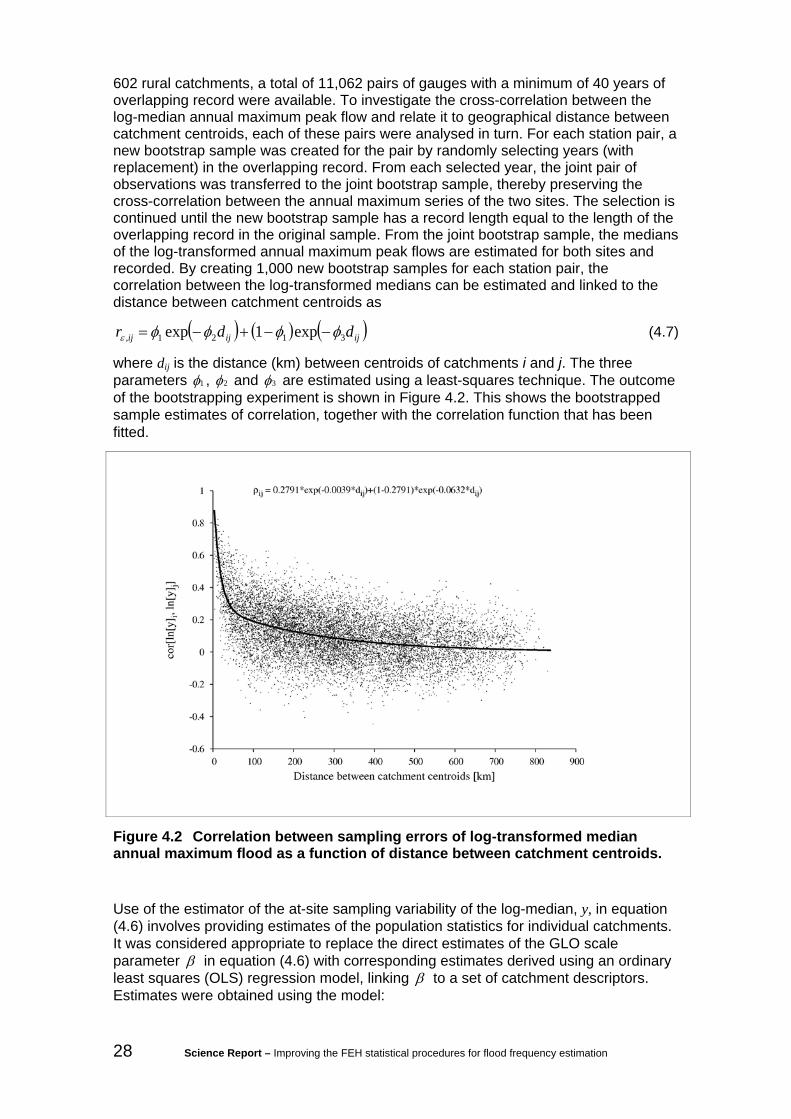
28 Science Report – Improving the FEH statistical procedures for flood frequency estimation
602 rural catchments, a total of 11,062 pairs of gauges with a minimum of 40 years of overlapping record were available. To investigate the cross-correlation between the log-median annual maximum peak flow and relate it to geographical distance between catchment centroids, each of these pairs were analysed in turn. For each station pair, a new bootstrap sample was created for the pair by randomly selecting years (with replacement) in the overlapping record. From each selected year, the joint pair of observations was transferred to the joint bootstrap sample, thereby preserving the cross-correlation between the annual maximum series of the two sites. The selection is continued until the new bootstrap sample has a record length equal to the length of the overlapping record in the original sample. From the joint bootstrap sample, the medians of the log-transformed annual maximum peak flows are estimated for both sites and recorded. By creating 1,000 new bootstrap samples for each station pair, the correlation between the log-transformed medians can be estimated and linked to the distance between catchment centroids as
( ) ( ) ( )ijijij ddr 3121, exp1exp φφφφε −−+−= (4.7)
where dij is the distance (km) between centroids of catchments i and j. The three parameters 1φ , 2φ and 3φ are estimated using a least-squares technique. The outcome of the bootstrapping experiment is shown in Figure 4.2. This shows the bootstrapped sample estimates of correlation, together with the correlation function that has been fitted.
Figure 4.2 Correlation between sampling errors of log-transformed median annual maximum flood as a function of distance between catchment centroids.
Use of the estimator of the at-site sampling variability of the log-median, y, in equation (4.6) involves providing estimates of the population statistics for individual catchments. It was considered appropriate to replace the direct estimates of the GLO scale parameter β in equation (4.6) with corresponding estimates derived using an ordinary least squares (OLS) regression model, linking β to a set of catchment descriptors. Estimates were obtained using the model:

Science Report – Improving the FEH statistical procedures for flood frequency estimation 29
[ ] [ ] i
P
ppipi x γααβ ++= ∑
=1,0 lnln (4.8)
where P is the total number of catchment descriptors used in the regression model, xi,p is the value of the p’th catchment descriptor for the i’th catchment, and pα is the p’th regression model parameter. Only a limited investigation has been made of the errors,
iγ . It should be noted that the results of the OLS regression are reported (Table 4.2) as if these errors can be assumed to be independent and normally distributed with mean zero and variance 2
γσ , whereas the errors are very likely to be correlated between catchments. Thus the estimates of the standard errors of the regression parameters are likely to be too small. The use of OLS estimates rather than GLS estimates at this stage is not thought to be important.
Table 4.2 Summary statistics for the regression model describing [ ]iβln which is used to model the variance of the sampling error of the median.
Variable Coefficient ( pα ) Standard error t-value p-value
Intercept ( 0α ) -1.1221 0.0664 -16.91 0.000Ln[AREA] -0.0816 0.0105 -7.78 0.000Ln[SAAR/1000] -0.4580 0.0401 -11.43 0.000Ln[BFIHOST] 0.1065 0.0520 2.05 0.041
28.0598107.0 22 === rdfγσ
The regression model has an r 2 value of only 28 per cent, which indicates less predictive power than could have been hoped for, but relates to the substantial sampling error in the estimates of the GLO scale parameters. To estimate the sampling covariance εΣ , estimates of β obtained through equation (4.8) are substituted into equation (4.6). Using these instead of the sample estimates of β substantially reduces the noise that would otherwise be included. The general effect of this unwanted noise is unclear. It is thought that it will have little effect on the performance of the estimated regression coefficients in the model for the log-median flood, but also that it could have a more important effect on the outcome of procedures for the use of donor sites (Chapter 5) in cases where these might be used for donor catchments with short records.
The outcome of the analysis summarised in Table 4.2 is a route to the construction of the covariance matrix of the sampling errors, εΣ , which plays an important role in the GLS procedure.
Model error
As the true values of QMED are unknown, properties of the model error cannot be estimated directly from the data in the same way in which properties of the sampling error were estimated. In the FEH, the existence of the model error correlation was acknowledged and set equal to the correlation between AMAX events using the formula
( )dr d 016.0exp, −=η , (4.9)
where d is the geographical distance (in km) between catchment centroids. While this might be a reasonable first approximation, the model error should ideally be estimated separately for each particular regression model under consideration rather than set to a

30 Science Report – Improving the FEH statistical procedures for flood frequency estimation
pre-defined value. The issue of a correct description of the model error correlation becomes an important issue when considering the effect of data transfer from donor catchments, as illustrated by Kjeldsen and Jones (2007), and discussed in detail in Chapter 5 of this report.
Therefore, a very important advance in the FEH methodology has been the development of an advanced recursive procedure to identify and specify a suitable model linking the model error correlation to the geographical distance between catchment centroids. An in-depth discussion of the method and application to the HiFlows-UK data set used in this study can be found in Appendix C and in Kjeldsen and Jones (2008). It was found that the relationship between model error correlation and geographical distance could reasonably be described using the same type of function as used to describe the correlation of the sampling errors, i.e. a mixture of two exponential functions:
[ ] ( ) [ ]ddr d 321, exp1exp ϕψϕϕη −−+−= , (4.10)
where 1ϕ , 2ϕ and 3ϕ are model parameters that must be estimated for each individual regression model.
Final estimation of regression parameters
Having specified the error structure, the regression model parameters can be estimated using a maximum-likelihood procedure, which incorporates what are essentially the steps involved in calculating the GLS estimates of the regression parameters. If it is assumed that the regression residuals are normally distributed with mean zero and a total covariance matrix, G2
ησ , described in equation (4.5), the objective of the overall estimation procedure is to minimise the negative log-likelihood function
( ) ( )[ ] ( ) ( ) ( )XθyGXθyG T −−+=−−122
21detln
21ln ηη σσkL (4.11)
with respect to the three model error correlation parameters ( 1ϕ , 2ϕ and 3ϕ ), the model error variance ( 2
ησ ) and the regression parameters (θ ). The problem is simplified by noting that, for given values of 2
ησ , 1ϕ , 2ϕ and 3ϕ (which between them determine G), the value of θ which minimises (4.11) is given the least squares estimator (specifically the GLS estimator)
( ) yGXXGXθ 1T11T −−−=ˆ . (4.12)
Thus, estimation by maximum likelihood can be implemented as a search over the four parameters 2
ησ , 1ϕ , 2ϕ and 3ϕ .
In reporting the results of the estimation, in particular for the uncertainties of the regression coefficients, the course adopted here has been to quote results from a final GLS analysis that is based on the optimised parameter values. The consequence of this is that the uncertainties reported (the standard errors and the implied tests of significance related to these) ignore the effects that derive from the estimation of the other parameters. This has the advantage of simplicity and should not prove too misleading in the present context where the uncertainties are used for guidance only. It also has the advantage of allowing a simple summary of the model which can be compared to the equivalent from other models. However, when undertaking the search of the variables to be included in the model for QMED, checks of the improvement (or otherwise) of the model by including selected candidate variables were made in the

Science Report – Improving the FEH statistical procedures for flood frequency estimation 31
form of a likelihood-ratio test comparing the optimised values of the log-likelihood (equation (4.11)) for models including and excluding the candidate. Thus the variable selection analysis has not relied on the approximation used to report and summarise the final model.
4.4 Variable selection Selecting the combination of catchment descriptors to be included in the final QMED model was a lengthy iterative process and, just as in the FEH, not every stage of the procedure is reported here. Throughout the process, the FEH QMED equation has been used as a benchmark against which other possible candidates could be judged.
4.4.1 The FEH QMED equation
The FEH QMED equation was developed based on a comprehensive analysis as reported in the FEH (Institute of Hydrology, 1999). For the present study, the first step in the search for an improved model was to re-estimate the parameters using the GLS method based on the 602 catchments taken from the HiFlows-UK dataset as desribed in Chapter 2. The summary statistics for the regression model are shown in Table 4.3.
Table 4.3 Summary statistics for the FEH regression model for ln[QMED].
Variable Coefficient ( pθ ) Standard error t-value p-value
Intercept 0.1066 0.1802 0.59 0.554Ln[AREA] 0.9775 0.0572 17.08 0.000Ln[AREA]2 -0.0122 0.0056 -2.16 0.031Ln[SAAR/1000] 1.7612 0.0913 19.29 0.000Ln[FARL] 3.7940 0.2753 13.78 0.000Ln[SPRHOST/100] 1.0864 0.0479 22.70 0.000RESHOST -3.7266 0.4020 -9.27 0.000
1543.02 =ησ , df = 595, r2 = 0.938 (log scale)
From the results in Table 4.3 it appears that the (ln[AREA])2 term added to the FEH QMED equation is less significant when estimating the QMED model using the updated HiFlows-UK data than with the dataset used in the FEH study (FEH, Vol. 3, Table 13.7). The rationale for adding the term was that early investigations of model residuals in the FEH study suggested a non-linear effect due to catchment size. A similar effect was not detected in this study, but rather a non-linearity effect due to catchment average annual rainfall, which was also evident from the residual plots reported in the FEH (Vol. 3, Figure 13.8), as will be discussed later.
4.4.2 Comprehensive search results
An exhaustive search procedure was used as a screening tool to identify potentially useful combinations of catchment descriptors. The search was based on ordinary least squares (OLS) rather than the more comprehensive GLS methodology developed in this study The search was restricted to a relatively small set of descriptors, where selection was based on the variables reported as most useful by the FEH study, together with the new descriptors developed for the present study. A summary of the results is presented in Table 4.4, and a discussion of these results follows.

32 Science Report – Improving the FEH statistical procedures for flood frequency estimation
Table 4.4 Best fitting OLS models using from one to 12 catchment descriptors
LnAREA lnSAAR lnBFIHOST BFIHOST lnFARL lnPROPWET lnDPSBAR lnFPEXT lnPRAT lnRMED(1day) lnEVAP R2
1 **** - - - - - - - - - - 0.520 1 - - - - - **** - - - - - 0.393 1 - - - **** - - - - - - - 0.301 2 **** - - - - **** - - - - - 0.818 2 **** - - **** - - - - - - - 0.804 2 **** **** - - - - - - - - - 0.794 3 **** **** - **** - - - - - - - 0.912 3 **** - - **** - - - - - **** - 0.904 3 **** - - **** - **** - - - - - 0.901 4 **** **** - **** **** - - - - - - 0.936 4 **** - - **** **** - - - - **** - 0.923 4 **** **** **** - **** - - - - - - 0.923 5 **** - - **** **** **** - - - **** - 0.941 5 **** **** - **** **** - **** - - - - 0.940 5 **** **** - **** **** - - - **** - - 0.940 6 **** - **** **** **** **** - - - **** - 0.944 6 **** **** **** **** **** - **** - - - - 0.943 6 **** **** **** **** **** - - - **** - - 0.943 7 **** **** **** **** **** **** - - - **** - 0.946 7 **** **** **** **** **** - **** - **** - - 0.946 7 **** - **** **** **** **** **** - - **** - 0.945 8 **** **** **** **** **** **** - **** - **** - 0.947 8 **** **** **** **** **** **** **** - - **** - 0.947 8 **** **** **** **** **** **** - - **** **** - 0.947 9 **** **** **** **** **** **** - **** **** **** - 0.948 9 **** **** **** **** **** **** **** - **** **** - 0.948 9 **** **** **** **** **** **** **** **** - **** - 0.947 10 **** **** **** **** **** **** **** - **** **** **** 0.948 10 **** **** **** **** **** **** **** **** **** **** - 0.948 10 **** **** **** **** **** **** - **** **** **** **** 0.948

Science Report – Improving the FEH statistical procedures for flood frequency estimation 33
Note that the two variables Ln[SPRHOST] and RESHOST used in the FEH QMED equation are not included in the results reported here although they did feature in earlier stages of this study. Previous studies (Kjeldsen et al. 2005) have found SPRHOST to be a less efficient descriptor of hydrological soil properties than BFIHOST, and RESHOST was found to lack a clear physical interpretation. Hence Ln[BFIHOST] and BFIHOST have been included as candidate descriptors in preference to the variables appearing in the FEH QMED equation.
The search procedure tests every possible combination of catchment descriptors by fitting the OLS regression and notes the resulting coefficient of determination (r2) for each combination. Table 4.4 shows the three best models, in terms of r2, that use from one to 10 different catchment descriptors
From the results in Table 4.4 it can be observed that the first five catchment descriptors (ln[AREA], ln[SAAR], ln[BFIHOST], BFIHOST and ln[FARL]) seem to occur more frequently in the model selection than the remaining descriptors. While it can be argued that ln[PROPWET] and ln[RMED(1day)] also occur relatively frequently, both these descriptors are highly correlated with ln[SAAR].
4.4.3 Investigation of residuals
Figure 4.3 shows some scatter plots that relate to development of the final model for QMED, in terms of selecting which descriptors should be included in the model equation and the form that this inclusion should take. Each scatter plot shows (on the y-axis) the residuals from a given model (fitted using GLS) plotted against (on the x-axis) selected individual catchment descriptors. In these plots, interest centres on the following features.
• The extent of any relationship between the residuals and descriptors not already included in the model, since this would indicate that that descriptor would improve the predictions.
• The possible presence of a curved pattern in the residuals when plotted against any descriptors (included or not in the model), since this would indicate the potential usefulness of considering other transformations of the descriptors.
The present study has examined more complete sets of such plots, but Figure 4.3 presents a simplified set that relates specifically to the final model selected, as described below.
The results from the initial analysis strongly suggest that a QMED equation based on the four descriptors ln[AREA], ln[SAAR], ln[FARL] and ln[BFIHOST] (row 3 in Figure 4.3) fits the data well without using too many spurious parameters. However, a visual inspection of the residuals from this particular model suggested a non-linear effect in the relation of the residuals to both ln[SAAR] and ln[BFIHOST]. Both of these effects were further investigated by estimating regression models of increasing complexity and plotting the resulting residuals against the different catchment descriptors, as shown in Figure 4.3. The first model in Figure 4.3 (row 1) is based on ln[AREA] only, and illustrates the need for including rainfall (SAAR), soil properties (BFIHOST) and upstream reservoir influence (FARL) in the model, as strong patterns can be observed when the model residuals are plotted against these catchment descriptors.

34 Science Report – Improving the FEH statistical procedures for flood frequency estimation
QMED Model lnAREA lnSAAR lnFARL lnBFIHOST BFIHOST SAAR−1
1.
lnAREA
2.
lnAREAlnFARL
lnBFIHOST
3.lnAREAlnSAARlnFARL
lnBFIHOST
4.lnAREASAAR−1
lnFARLlnBFIHOST
5.lnAREASAAR−1
lnFARLlnBFIHOSTBFIHOST
6.lnAREASAAR−1
lnFARLBFIHOST2
++++
+++ ++
+++++ +++
+++++
++ +++++++++++
+++++++
++
+++
++
+++
+
++
++++
++++
+++++ ++
++++
+
+ + +++++
++
+++ +++
++++
++
++++
++
++
+++ ++
++
++
+++
+
+ ++++ +
+
+
++
++++
++
++++
+ +
++ +
+++
+
+
++
++++
+ +
+++
++
++ ++
++++
+++
++
+ + +++
+ +
++
++
+
+
+
++++
+
+
+
+
+++
+
+
++++++ ++
+
++++ + ++ ++
+ ++
+ ++++++++++++
++
+++
++
++
+++
++ ++ +
+++++++
+
++++
+
++ +
++++
+
+++
+
++
+
+
+
+++++
+
++
++
++
+
+
++ +
+++++++++++ +
+
++++ ++++++
++
++ + +++
+++
++++
++
+
+++
+
+
++ ++
+++
++ +++
+
+
+
++++++++
++++
+++++
+ +++
+++
+
+
+++
++ +
++++
+++
++
+
+
++ +++
++++ ++++ +
++++
++++
++++
+++
++++
++
++++
+++
++ ++
++
+
+
+
+
+++
++
+++
+
++
+
+
++ +
++
++++ +++
++
+
++
+
+ +
+ +
++
+ ++
++ ++++
++++++++
+++ + +++
++
+++ +
+ +++
++ +
++++
+++
+++++
++
+++++ ++ +
+
++
++
++
++
+++
++
+
+++++++ +++
++++++
++++++
++++
+ +++
++++
++
+
++
++
+
+
+
+
+
++
++
+ ++
+
+++
++
++
+++++++++
++
+++++++++
+++++
+
+
+
+
+++++
+
+
++++
++++ +++
+++
+
+
+
+++
++
++
+++
+++ +
+++ ++ +
+++
+
++++++ ++
+++
+
++++
+ ++++ ++
+
+
+
++
+++ +
+++
++
+
+
+ +++++
+
+
+++
+++
+
++ ++
++++
+
++
+++
++++++
++
++ ++
++++++++
+++
+
+++++
+
+++++
+
+ +++++++ + ++ +
++ +
++ ++
++
+
+++++++ ++
++++
++
++++
+++
++++
++++
++
+
+++
+
++
+++
++
+
+
+ +
+
++
+
+
++++++
+++ ++
+
++
+
++
+++++++
+++
+++
+
++++
++++++
++
++
+ ++++
+
++
+++
++ ++++
+
+
++
+++
++++
+
+
++
+
+
+++++++
++++
+
++
+++
+ +++
+++
+
+
+++
++ +
++
+
+
+
++++
+
+
++++
+
++++
+++
+ ++
+++
++++
+
+++
+++
++
++++
++++
+++
++ +
+
++
++
++
+ ++++
++
++
++
+
+
++ +
++
+++++
++
+
+
+
+
+
+
+ +
+
+
+
+
+ ++
++
+++
+
++
++
+++
+
++++ +
++
+
+
+
++ +
+ ++ ++
+ +
+
+++
+++++
+++++ +++
++
+
++
+
+
+
++
+
++ +
++
+++
+
+
++++++ +++
+
++
+++
+++
++++++
++ ++
++
+++
++
+
++++++++
+ +++
+
++
+
+
++
+
++
++
+++++++++
++
+++
+
+++++ ++
++++
++
++
+++++
+
+++
+++++
+++
++
++
++
+++
+
+++
+++ ++++
+
++ ++ +++++
+++++
+ ++++++
++
+
++ ++
++ +
+
+
+
+
+++
++ ++++
+
+
+
++ ++
++ +
+
++
+++++ +++ + +
+++
++
++
+++
++++++
++
++ ++
+++++++
+
+++
+
++
++
+
+
+++++
+
+ ++
+
++++ + ++
+++
++
+++
+++++++++
++
++
++
+
+++
+
+ ++
+ +
++++
+++++
+
+
++
+
+
++
+
++
++
+
+
+ +
+
++
+
+
+
+++++
+
+
+ ++
+
++
+
++
+ ++
++++++
++
+
+
+
+++
+++
++++
++
+
+
+ +++
++
++
++
+
+++
+
+
++
++
++++ ++
++
+
+
+
+++
++++
+++
+++
+
+
+
+++++
+++
++
+
+
++
+++
+ ++
+
+ +
+
++++ +
+
++ +++++++
+
+
+
++
++++ ++
++
+
++
+
+++
++
++++
++
+++++
++
++ +
+
++++
+ ++
++++ ++ +
++
+++ +
++++++ +++
+++
+
+
+
+ ++++ +
++
++
+ +++
+++
++
+++++++
+ +++
+
++++ +
+ ++ ++
+ +
+
++++++++++
+++
+++++ ++ ++
+++
+ +++
++++++
+
++++
++
+ +++
+
++
++++
++
+++
+++
++ ++++++
+
+ ++
+++++
+++
+ +++
+
+
++
+
++
+
++
++
++++
++++++
+
+++
+
+++++ +++
+++++
++
+++++
+++
+
+++++
+++++
+
+
++
+++
+
+
++
+++
+++
+
+++ +
+ +++++++
+++
+ ++++++++
+
++ +
+
++ +
+
+
+
+
+++
++ ++++
+
+
+++ +
+
++ +
+
++
++++
+++
+ + ++
+++
+
++
+++
++++
++
++
++ ++
+++++++
+
+++
+
++
++
+
+
+
++++
+
+ ++
+
++++
+ ++
+++
++
+++
+++++++
++
++
++
++
+
+++
+
+ ++
+ +
+ +++++++
+
+
+
++
+
+
++
+
++
++
+
+
+ +
+
+++
+
+
+++++
++
+ ++
+
++
+
++
+ ++
+++++
++
++
+
+
+++
+++
++++
++
+
+
+ +++
++
+
+++
+
+++
+
+
++
++
++++ ++
++
+
+
+
+++
++++
+++
+++++
++++++
+++++
++
++
+++ + ++
+
++
+
++++ +
+++ ++++
+++
+
+
+
++
++++
++++
+
+++
+++
++
++++
++
++++
+
+++
+ ++
++++
+ +++++
++++
++
+++
+++++++ +++
+
++
+
+
+
+ +++
+ ++ +++
+ +++
+ ++++
++++ +++ + ++
+
+
++++ +
+ ++ ++
+ +
+
++++++++++++++++
++
++ ++
+++
+ +++
++++++
+
++++
++
+ +++
+
+
+++++
++
+++
+++
++ ++++++
++ +
+
++++
+++
+
+ +++
+
+
++
+
++
++
+
++
++++
+++++++
+++
+
+++++ ++
++++
+++
++
++++
++
++
+++++
+++
++
+
+
+ +
+++
+
+++
+++
+++
++++ +
+ ++++++++
+++ +
++++
+++
++
+++++ ++ +
+
+ +++
++ +
+++
+
+
+++ +
+
++ ++
+
+
+++++
++
+
+++
++ ++ ++
++
+
+
++++
+
++++
+
+
+++++++
+
+++
+
+++
+
++ ++++++
+ +
++++++ + ++ ++
++
++
++
+++++++++
++
+++
++
+++
+
+ ++++
+
+++
++++
++
+
+++
+
++
+++
++
++
+
+
+
++ ++++
++
++
+
+
+++
+
++
+
+
+
+
++
+++++
+
+++
+
+
++++
++++
++
++
+
+
+ +++
++
+
+++
+
++
+
+
+
+
+
++
++++ ++
++
++
+
+ +++
+++
+++
+++
+
+++++++ +++
++
+++++++ +++
+
++
+
++++ +
+++
+++++++
+
+
+
++
+
+++++++
+
+++
+++
++
++++
++
++++
+
+++
+ ++++
++
++
+++
++ ++
++
+
+++
+++++
++ +++
++
+
++
+
+ +++
+ ++ +++
+ +++
+ ++++
++++ ++++ +++
++
+++ ++ ++
++
+ +
+
+++
++
+
+++++
++ +++++ ++ +
+++
+
+ ++
+
+++
+++
+
++++
+++ ++
+
++
++++++
++
++
+
+
+++
++++
+++
+ +
+
++++
+++
+
+ +++
+
+
++
+
++
+
++
++
++++
+++++++
+++
+
+++++ ++
++++
+++
++
++++
+++
+
+++++
+++
++
+
+
+ +
+++
+
+++
+++
+++++++ +
+ ++++++++
++
+ ++++++
++
+++ ++
++ +++
+
+ +++
++ +
+++
+
+
+++ +
+
++ +
+
+
+
+++++
+++
+ ++
++ ++ ++
++
+
+
++++
+
++
++ +
+
+++++++
+
+++
+
+++
+
++++++++
+ +
++++++ + +
+ +++
++
+++
+++++++++
++
+++
++
+++
+
+ ++++
+
+++++++
++
+
+++
+
+++++
++
++
+
+
+
++ ++++
++
++
+
+
+++
+
++
+
+
+
+
++
++++
+
++++
+
+
++++
++++
++
++
+
+
+ +++
++
+
+++
+
++
+
+
+
+
+
++
++++ ++
++
++
+
+ +++
+++
+++
+++
+
+++++++ +++
++
+++++++ + ++
+
++
+
++++ +
+++ +++++++
+
+
+
++
+
+++++++
+
+++
+++
++
++++
++
++++
+
+++
+ ++
++++
++
+++
++ +++
++
+++
+++++
++ +++
++
+
+
+
+
+ +++
+ ++ +++
++
++
+ ++++
++++ ++++ ++++
++++ ++ ++
++
+ +
+
+++
++++++++
+++++
++ ++ +
+++
+
+ ++
+
++++++
+
++++
+++ ++
+
++
++++++
++
++
+
+++
++++
+++
++ +
+
++++
+++
+
+ +++
+
+
++
+
++
+
++
++
++++
+++++++
+++
+
+++++ ++
++++
+++
++
++++
+++
+
+++++
+++
++
+
+
+ +
+++
+
+++
+++
+++++++ +
+ ++++++++
++
+ ++++++
++
+++ ++
++ +++
+
+ +++
++ +
+++
+
+
+++ +
+
++ +
+
+
+
+++++
+++
+ ++
++ ++ ++
++
+
+
++++
+
++
++ +
+
+++++++
+
+++
+
+++
+
++++++++
+ +
++++++ + +
+ +++
++
+++
+++++++++
++
+++
++
+++
+
+ ++++
+
+++++++
++
+
+++
+
+++++
++
++
+
+
+
++ ++++
++
++
+
+
+++
+
++
+
+
+
+
++
++++
+
++++
+
+
++++
++++
++
++
+
+
+ +++
++
+
+++
+
++
+
+
+
+
+
++
++++ ++
++
++
+
+ +++
+++
+++
+++
+
+++++++ +++
++
+++++++ + ++
+
++
+
++++ +
+++ +++++++
+
+
+
++
+
+++++++
+
+++
+++
++
++++
++
++++
+
+++
+ ++
++++
++
+++
++ +++
++
+++
+++++
++ +++
++
+
+
+
+
+ +++
+ ++ +++
++
++
+ ++++
++++ ++++ ++++
++++ ++ ++
++
+ +
+
+++
++++++++
+++++
++ ++ +
+++
+
+ ++
+
++++++
+
++++
+++ ++
+
++
++++++
++
++
+
+++
++++
+++
++ +
+
2 4 6 8
++++
++++
+++
+++ ++
+
++ ++++++++
+++++++
+
+++++++
++
++ +
++
+++
+
++
++++
++++
++++++ +
++++
+
+++++++
++
+++++
++
+++
++++++
++
++
+++++
++
++
++ +
+
++++++
+
+
++
++++
++
++++
++
++ +++
++
+
++
++++++
+ ++++
++++
+++
++++++
+++++++
++
++
+
+
+
+++++
+
+
+
+++
+
+
+++
+++++
+
++++++++++++++++++++++++++++++
++
++
+++
+++++
+++++++
+
++++
+
+++
++++
+
+++
+
+++
+
+
+++++
+
++++
+++
+
+++
++++++ +++ ++++
++++++++++
++
++++++
+++
++
+++
++
+++
+
+
++++
+++
+++ +++
+
+
+++++++
++
+++
+++
++++ +++
++
+
+
+++
+++
++++
+++
++
+
+
+++++
++++++
++ ++
++++
+++++++
+++++++
+++++ +
++
+
++ ++
++
+
+
+
+
+++
++
+++
+
+++
+
+++
++
++++ ++++
+
+
++
+
++
++
++
+++
++++
++
++++++
+ ++ +++++
++
+
++++++
++++++
+++
+++
+++++
++
++++++++
+
++
++++
++
+++
++
+
+ ++++++
+++
+++++++++++++
+++++++
++++
+++
++
++
+
+
+
+
+
++
++
+ ++
+
++ +
++
++++
+++++++++
+++++++
++
++ ++ +
+
+
+
+
+++++
+
+
++++
+++++ ++
+++
+
+
+
+++
++
++
++ ++
+++
++++++
+++
+
+++++
++++
+ +
+
++ ++
+++ ++++
+
+
+
++
++++
+++
++
+
+
+ +++ ++
+
+
+++
++ +
+
+ ++++++
+
+
++++
+
+++++
+
++
+++++++++++
+
+++
+
+++++
+
+++++
+
+++++++++++++++++++
++
+
+++++++++
++++
++
++++
++++
++
+++++
++
+
+++
+
+++
++
++
+
+
++
+
+++
+
++++
++
++
+++
+
++
+
+++
++++++ +++
+++
+
++++
+++++++
+
++
+++ +++
++
+++
++++
++
+
+
++++
+++
++
+
+
++
+
+
+++++++
++++
+
+ +
+++++
+++ +
+
+
+
+++
+++
++
+
+
+
++++
+
+
+++++
++++++ ++ +
+
+++
+++++
+++
++
+++
++
+++++
+
++
+
++ +
+
++
++
++
+++++
++
++
+++
+
+++
++
+++++++
+
+
+
+
+
+
++
+
+
+
+
++ +
++
++
++
++++
+++
+
+++
++++
+
+
+
+++
+++++++
+
+++
+ ++++
++++++++
++
+
++
+
+
+
++
+
+++
++
+++
+
+
++++ +++++
+
++++++
++
+++++
+++++
+++++
++
+
++ +++ ++
+
++++
+
++
+
+
++
+
++
++++++++++++
+
+++
+
+ +++
+ +++
+ + ++
++
++
++++
+
+++
+++++
+ ++
++
++
++
+++
+
+++
++ +++++
+
+++++
+++++ ++++
+++ ++ ++
++
+
+ +++
+++
+
+
+
+
++++++ +++
+
+
+
++ ++
+ ++
+
++
+++++++ ++++
++++
++++
+
+++++
+
++
+++++++++++
+
+++
+
++++
+
+
+++++
+
+++
+
+++++++++++++++
+++++++++
++++++
+
++
+
+
+++++
++
++
+++++
+
+
++
+
+
++
+
++
++
+
+
++
+
+++
+
+
+++++
+
+
+++
+
++
+
+++ ++
+++++
++
++
+
+
+++
+++++++
++
+
+
+++ +
++
++
++
+
+++
+
+
++
++
+++ +++++
+
+
+
++ +
+++++++
+++
+
+
+
++++++
+++ +
+
+
++++ +
+++
+
+ +
+
++++ +
+
++++ ++
+++
+
+
+
++
+++++ +
++
+
++
+
++
+++
++++
++
+ +++
+
++
+++
+
++
+ ++++
++ +++ ++
++
++++
++++++ +
+++
++
+
+
+
++++ ++
++
++
+++
+
+++++
+++ ++ ++
++++
+
++
+++
+++++++
+
++++ ++++++++
+
++++ ++ ++
+
++ +
++++
++++ +++
++
+++
+
++++
+
++++++
++
+++
+++++++
+++++
+++
++++
++++
++++
+
+
++
+
++
+
++
++++++
++++++
+
+++
+
+ +++
+ ++ ++ + +
+++
++
++++
++++
+++++
+ +++
+
+
+
++
+++
+
+
++
++ ++++
+
++++
+++++++ ++++
+++ ++ ++++
+
+++
+
+++
+
+
+
+
++++++ +++
+
+
+++ +
+
+ ++
+
++
+++++
+ +++++
++++
++++
+
++++
++
++
++++
+++++++
+
+++
+
++++
+
+
+
+++++
+++
+
+++++++++++++++
+++++++++
++++++
+
+++
+
+++++
++ +++++++
+
+
++
+
+
++
+
++
++
+
+
++
+
+++
+
+
+++++
++
+++
+
++
+
+++ ++
+++++
++
++
+
+
+++
+++++++
++
+
+
+++ +
++
+
+++
+
+++
+
+
++
++
+++ +++++
+
+
+
++ +
+++++++
+ ++++
+++++++ ++
+ +
++
++++ ++++
+
++
+
++++ +
+++
++ ++++
+
+
+
+
++
++++
+ +++
+
+++
++
+++
++++
++
+ +++
+
+++
++ +
++
+ +
+++
++ ++
+ ++
++
+++
+ ++++++ +
++
+
++
+
+
+
++++
++++ +
+
+++
+
+++++
+++ ++ +++++
+
+
++
+++
+++++++
+
++++ ++++++++ +
++++
++ ++
+++
+++++
++++ ++
+
++
+++
+
++++
+
+
+++++
++
+++
++++++++++++
+++
++ ++
++++
++++
+
+
++
+
++
++
+
++++++
+++++++
+++
+
+ ++++ ++
++ + +
+++
++
++++
++++
+++++
++
++
+
+
+
++
+++
+
+++
++ +++
++
++++
+++++
++ ++++
+++ ++ +
+++
++
+++ +++++
+
+ ++++++
+++
+
+
+++ +
+
+ +++
+
+
+++++
++
+
+++
++++++
+++
+
+++++
+++++
+
++
+++++
+
+++
+
+++
+
++++
++++
++
++
+++++++++++++++
+++++++++
+++++
++
+++
+
++++
++
+ ++
++++
++
+
+++
+
+++++
++
++
+
+
+
++++++++
+++
+
+++
+
++
+
+
+
+
++
+++++
+
+ ++
+
+
++++
++++
++
++
+
+
+++
+
++
+
+++
+
++
+
+
+
+
+
++
+++ +++++
++
+
++ ++
++++++
+ ++
+
++
++++++ ++
+ +
++ ++++ ++
++
+
++
+
++++ +
+++
++ ++++++
+
+
++
+
++++
+++
+
+++
++
+++
++++
++
+ +++
+
+++
++ +++
++
++
+++
+++ +
+++
+++
+++++
++ +
+++
++
++
+
++++
++++ +
+
+++
++++
++
+++ ++ +++++++
++
++++++
++++
+
+++
++
+
+++++
+ +++++++++
+++
+
+++
+
+++
+++
+
++
+++
++++
+
++
++++++
++++
+
+
++++++
++++
++
+
++ ++
++++
++++
+
+
++
+
++
+
++
++++++
+++++++
+++
+
+ +++
+ +++
+ + +++
+++
++++
++++
+++++
++
++
+
+
+
++
+++
+
+++
++ ++++
+++++
+++++
++ ++++
+++ ++ ++
++
++ +++
++++
+
+
+ ++++++
+++
+
+
+++ +
+
+ ++
+
+
+
+++++
+ ++
+++
++++++
+++
+
+++++
++
+++
+
++
+++++
+
+++
+
+++
+
++++++++
++
++
+++++++++++++++
+++++++++
+++++
++
+++
+
++++
++
+ ++++++
++
+
+++
+
+++++
++
++
+
+
+
++++++++
+++
+
+++
+
++
+
+
+
+
++
++++
+
++ ++
+
+
++++
++++
++
++
+
+
+++
+
++
+
+++
+
++
+
+
+
+
+
++
+++ +++++
++
+
++ ++
++++++
+ +++
++
++++++ ++
+ +
++ ++++ +++
+
+
++
+
++++ +
+++
++ ++++++
+
+
++
+
++++
+++
+
+++
++
+++
++
++
++
+ +++
+
+++
++ +
+++
++
+
+++
+++ ++
++
+++
+++++
++ +
+++
++
+
+
+
++++
++++ +
+
+++
++++
++
+++ ++ +++++++
++
++++++++++
+
+++
+ ++
+++++
+ +++++
++++
+++
+
+++
+
++++
+++
+ ++++
++++
+
++
++++++
++++
+
+++++++
++++
++
+
++ ++
++++
++++
+
+
++
+
++
+
++
++++++
+++++++
+++
+
+ +++
+ +++
+ + +++
+++
++++
++++
+++++
++
++
+
+
+
++
+++
+
+++
++ ++++
+++++
+++++
++ ++++
+++ ++ ++
++
++ +++
++++
+
+
+ ++++++
+++
+
+
+++ +
+
+ ++
+
+
+
+++++
+ ++
+++
++++++
+++
+
+++++
++
+++
+
++
+++++
+
+++
+
+++
+
++++++++
++
++
+++++++++++++++
+++++++++
+++++
++
+++
+
++++
++
+ ++++++
++
+
+++
+
+++++
++
++
+
+
+
++++++++
+++
+
+++
+
++
+
+
+
+
++
++++
+
++ ++
+
+
++++
++++
++
++
+
+
+++
+
++
+
+++
+
++
+
+
+
+
+
++
+++ +++++
++
+
++ ++
++++++
+ +++
++
++++++ ++
+ +
++ ++++ +++
+
+
++
+
++++ +
+++
++ ++++++
+
+
++
+
++++
+++
+
+++
++
+++
++
++
++
+ +++
+
+++
++ +
+++
++
+
+++
+++ ++
++
+++
+++++
++ +
+++
++
+
+
+
++++
++++ +
+
+++
++++
++
+++ ++ +++++++
++
++++++++++
+
+++
+ ++
+++++
+ +++++
++++
+++
+
+++
+
++++
+++
+ ++++
++++
+
++
++++++
++++
+
+++++++
++++
++
+
−0.5 0.0 0.5 1.0
++++
+++ +
++++
+++++
++++ +
+ ++++++++++++
+++++++++
+++
++
++ +
+
++
+++++++++
+++ +++
++++
+
++ +++++
++
+++ ++
+++++++++++
++++++++
+++++
++ +
+
++++++
+
+
++
+ +++++
++++
++
++++++
+
+
++
++++++
+++
+++++ +
+++
++
+++
+
+++++++
++
+ +
+
+
+
+++++
+
+
+
+++
+
+
++++++++
+
++++++++++++++++++ +++++++
+++++
++
++
+++
+ ++++
++++
+ ++
+
++++
+
+++
++++
+
+++
+
+++
+
+
+++++
+
++
++
++
+
+
+ ++
++++++++++++
+
++++++++++
++
++++++++
+
++++++
+
++ +
+
+
+++++++++++++
+
+
++++++++
++ +
++
++++++++
+++
+
+
++
+
+++
++++
+++
+ +
+
+
+++++
++++++++++
++++
+ ++++++++++++++
++++++
++
+ ++ +
++
+
+
+
+
++
+
++
+++
+
+++
+
+ ++
++
+++++++++
+
++
+
++
+ +
++
+++
++ + +
++
++++++++
+++ ++++++
+++++++++++++++
++++
++++++++++
+ ++ +
+
++
++
+++
+
+++
+ +
+
+ +++++ +
+++
++++++++++++++
+++++++
+++
++
+
++
++
+
+
+
+
+
+++
+
+++
+
+++
++
+++++++++++++
+++++++++
+++ ++
+
+
+
+
++ ++
++
+
++++
+++ +++++++
+
+
+
+++
++++
+++++++
+++++++++
+
++++++++
+++
+
++ ++++++++ +
+
+
+
++
+++++++
++
+
+
++++++
+
+
++ ++++
+
++++
++++
+
+++++
++++ +
+
++
++++++ ++++++
+++
+
+++++
+
++ ++++
+++++++++++++++++++
++
+
+++++++++
++++
++
++++
+ ++
++++
++
++
++
+
+++
+
++++
+
++
+
+
++
+
+++
+
+++++
+
+++++
+
++
+
+++++++++
++++++
+
++++
+++++++
+
++
++++++
+++++++++
+ +
+
+
+++++++++
+
+
++
+
+
+++++++
+++ +
+
++
+++++
+ ++++
+
+
++
+
+++++
+
+
+
+++
+
+
+
+++++
+++++
+++++
+++
++
+++
+++
+++++
+++
++++
+
++
+
+++
+
++
++
++
+++++
++
++
+++
+
+ ++
++
+++++++
+
+
+
+
+
+
++
+
+
+
+
+++
++
++
++
++
++
++ +
+
+++
++++
+
+
+
++++++++++
+
+++
++++
++++++++++
++
++
+
+
+
++
+
+++
++
++ +
+
+
+++++ ++++
+
++++++++
++++++++++
++
+++++
+
++ +++++
+
+ +++
+
++
+
+
+++
++
+++++++++++++
+++
+
+++++++
+++ +
++
++
+++ ++
+
+++
+++
+ ++++++++
++
+++
+
+++
+++ ++++
+
++++++++++++++
+++++++
++
+
++++
+++
+
+
+
+
+ ++++++++
+
+
+
++++
+++
+
++
+ ++++++++
+++
++
+
+++++
+++
+ ++
++
+++++++++++
+
+++
+
++++
+
+
++ ++++
+++
+
+++++++++++++
++
+++
++++++
++++++
+
++
+
+
+ ++
++
++++
+ ++ ++
+
+
++
+
+
++
+
++
++
+
+
++
+
+++
+
+
++++
+
+
+
+++
+
++
+
+++++
+++++
++++
+
+
++++++++++
++
+
+
++++
++
++++
+
+++
+
+
++
++
++++++++
+
+
+
+++
+++++++
+++
+
+
+
+ +++++
++
++
+
+
+++
+++++
+
++
+
+++ ++
+
+++++++++
+
+
+
+++
+++++++
+
++
+
+++++
+++
+
++
++ ++
+
++
++++
++++++
+
+++++++
++
++++++ +++
+++++++
+
+
+
++++++
+++
+
+ ++
+
+++++
++ +++++
++++
+
++
++++++++++
+
+++
++++++++++
+++++ ++ ++
+++++ ++
+++ ++ +
+
+++++
+
++++
+
+++++++
+++
+
++
+++++
+ +++
+
+++
++++
+++
+
+ +++
+
+
++
+
+++
++
+++++++++++++
+++
+
++++++++++ +
+ ++
++
++ ++
++++
+++
+ ++++++
+
+
++
+++
+
+
++
++++++
+
+++++++++++++++
+++++++++
+
+++
+
+++
+
+
+
+
+ ++++++
+++
+
++++
+
+++
+
++
+++++
++++
++++
++
+++++
+++
+++
++
++++
++ +++++
+
+++
+
++++
+
+
+
++++
+
+++
+
+++++++++++++
++
+++
++++++
++++++
+
+++
+
+ ++
++
+++++ ++ +
+
+
+
++
+
+
++
+
++
++
+
+
++
+
+++
+
+
++++
+
++
+++
+
++
+
+++++
+++++
++++
+
+
++++++++++
++
+
+
++++
++
+
+++
+
+++
+
+
++
++
++++++++
+
+
+
+++
+++++++++++++
+ ++++++ +++
++++++++++
+
++
+
+++ ++
+++
+++++++
+
+
+
+++
+++++++
+
+++
+++++
+++
+
++
++ ++
+
+ ++
+++
++++
+++
++++
+++++
++++++ +++
++++
+
++
+
+
+
++++
++ ++++
+ ++
+
+++++
++ ++ +++ ++++
+
++
++++++++++
+
+++
++++++++++++++
+++ ++
+ ++++ ++
+++ ++ +
+
+++++
+
++++
+
+
++++++
+++
+
++
++++++ ++
++
+++
++ ++
+++
+
+ +++
+
+
++
+
+++
++
+++++++++++++
+++
+
+++++++
+++ +
+ ++
++
++ ++
++++
+++
+ ++
++++
+
+
++
+++
+
+++++++++++++++++++
+++++++++++++
+++++
+++++ ++
+
++ +++++++++
+
++++
+
++++
+
+
+ ++++
+++
++ +
+++ +++
+++
+
+++ ++
+++++
+
++
++++
++
+++
+
+++
+
++ +++++
+
++
+++++++++++++++
++
+++++++++
+++++
++
+++
+
+ ++ +
++
+++
+ +++++
+
+++
+
+++++
++
++
+
+
+
++++++++
+++
+
+++
+
++
+
+
+
+
++
+++++
+
+++
+
+
++++++++++
++
+
+
++++
++
+
+++
+
++
+
+
+
+
+
++
++++++++
++
+
++++
++++++++
+
+
++
+ ++++++ +
++
++++++++++
+
++
+
+++
+++++
++++++++
+
+
++
+
++++
+++
+
+++
+++++
+++
+
++
++ ++
+
+ ++
+++++++++
+++
++++
+++
++++++ +++
++++++
+
++
+
++++
++ ++++
+ ++
++++
++
++ ++ +++++++++
+++++++
++++
+
+++
++
+
+++++++++++
+ ++ +
++ +
+
++ +
+
+++
++ +
+
+++++
+++++
++
++++++
+++
+
+
+
+++++++
+++
++
+
++ ++
+++
+
+ +++
+
+
++
+
+++
++
+++++++++++++
+++
+
+++++++
+++ +
+ ++
++
++ ++
++++
+++
+ ++
++++
+
+
++
+++
+
+++++++++++++++++++
++++++
+++++++++
+++++++
+ ++
+
++ +++++++++
+
++++
+
+++
+
+
+
+ ++++
+++++++++ +++
+++
+
+++ ++
++
+++
+
++
++++
++
+++
+
+++
+
+++++++
+
++
+++++++++++++++
++
+++ ++++++
+++++
++
+++
+
+ ++ +
++
++++ ++
+++
+
+++
+
+++++
++
++
+
+
+
++++++++
+++
+
+++
+
++
+
+
+
+
++
++++
+
++++
+
+
++++++++++
++
+
+
++++
++
+
+++
+
++
+
+
+
+
+
++
++++++++
++
+
++++++++++++++
++
+ ++++++ +
++
++++++++++
+
++
+
+++
+++++
++++++++
+
+
++
+
++++
+++
+
+++
+++++
+++
+
++
++ ++
+
+ ++
+++
++++++
+++
+++++++
++++++ +++
++++++
+
+
+
+
++++
++ ++++
++
+++++
++
++ ++ ++++++++
++
++++++++++
+
+++
+++
+++++++++++
+ ++ +
++ +
+
++ +
+
+++ +
+ ++
+ ++++
+++++
++
++++++
+++
+
+
++++++++
+++
++
+
++ ++
+++
+
+ +++
+
+
++
+
+++
++
+++++++++++++
+++
+
+++++++
+++ +
+ ++
++
++ ++
++++
+++
+ ++
++++
+
+
++
+++
+
+++++++++++++++++++
++++++
+++++++++
+++++++
+ ++
+
++ +++++++++
+
++++
+
+++
+
+
+
+ ++++
+++++++++ +++
+++
+
+++ ++
++
+++
+
++
++++
++
+++
+
+++
+
+++++++
+
++
+++++++++++++++
++
+++ ++++++
+++++
++
+++
+
+ ++ +
++
++++ ++
+++
+
+++
+
+++++
++
++
+
+
+
++++++++
+++
+
+++
+
++
+
+
+
+
++
++++
+
++++
+
+
++++++++++
++
+
+
++++
++
+
+++
+
++
+
+
+
+
+
++
++++++++
++
+
++++++++++++++
++
+ ++++++ +
++
++++++++++
+
++
+
+++
+++++
++++++++
+
+
++
+
++++
+++
+
+++
+++++
+++
+
++
++ ++
+
+ ++
+++
++++++
+++
+++++++
++++++ +++
++++++
+
+
+
+
++++
++ ++++
++
+++++
++
++ ++ ++++++++
++
++++++++++
+
+++
+++
+++++++++++
+ ++ +
++ +
+
++ +
+
+++ +
+ ++
+ ++++
+++++
++
++++++
+++
+
+
++++++++
+++
++
+
−0.4 −0.2 0.0
++++
+++++++
+++ ++
+
++++++++++++++++++
+++++++
++
+++
++
+++
+
++
++++
++++
+++
+++++
+++
+
++ ++++ +
++
+++++
++
+++
++++
++
++
++
+++++
++
++
+++
+
+ +++++
+
+
++
++++
++
++++
++
+++
+++
+
+
+++
+++++
+++
++
++++
+++
++
++++
+ +++ +
++
++
++
+
+
+
++
+++
+
+
+
+++
+
+
++
+++ +++
+
+++
++++++++
+++++++ ++ ++++
++
++++
++
++
+++
+++++
++ ++
+ ++
+
+++ +
+
+++
++++
+
+++
+
++
+
+
+
+++++
+
++
++
+++
+
+ ++
+++++++++++++
++++++++++
++
++ ++++
+++
++
+++
++
+++
+
+
++++
+++
++++++
+
+
+++++++++
+++
+++++
++++
++ +
+
+
++
+
+++
++++
+++
+ +
+
+
+++++
++++++
+ ++++++
+++++
++++++
++++++++++++
+
++++
++
+
+
+
+
++
+
++
+ ++
+
+++
+
++ +
++
+++++++
++
+
++
+
++
++
++
+++
++++++
++++++
++++++++
++
+
+++ +++++
++++++
++
+++++++
++
+++++++++
++
++++++
+++++
+
+ + +++++
+++
+++++
+++++++
++
+++ +
++++ ++
++
+
++
++
+
+
+
+
+
++
++
+ ++
+
+++
++
+++++++++++
++
+++++++ +
++++
++
+
+
+
+
++ +++
+
+
++++
+++++++
+++
+
+
+
+++
++
++
++++++ +
++++++
+++
+
+++++++++
++
+
++++
+ +++++ +
+
+
+
++
+++ ++++
++
+
+
+++
+++
+
+
++ +
++ +
+
++++
++++
+
++++
+
++ +++
+
++
+++++ +++ +
+ ++
++ +
+
++++
+
+
+++++
+
+++ +++ ++++++
+++
++++
++
+
++ +++++ + +
+++
+
++
+ +++
+++
++
++
++
++
++
+
+++
+
++
+++
++
+
+
+ +
+
++
+
+
++++
++
+++++
+
++
+
+++
++++++++++++
+
+++ +
++++++
++
++
+++ +++
++
+++
+ +++
++
+
+
++
+++
++++
+
+
++
+
+
+++++++
++ +++
++
+++
++++
+++
+
+
++
+
+++
++
+
+
+
+++
+
+
+
+++++
+++++++ ++
+
+++
++++
+
+++
+++
++
+++++++
+
++
+
+++
+
++
++
++
+ ++++
++
++
+++
+
++ +
++
+++++++
+
+
+
+
+
+
++
+
+
+
+
+++
++
+++
+
++++
++ +
+
+++++
+ +
+
+
+
++ ++++ ++++
+
+++
+++
++
+++++ +++
++
+
++
+
+
+
++
+
+++
++
+++
+
+
+ +++++ +++
+
++
++++
++
+++++
+++ + +
+++
+++
+
+
++ ++++++
+++ +
+
+++
+
++
+
++
+++++++++++++
+++
+
+++ +
++++
+++++
++
+++++
+
+++
+++
++++
++++
+
++
+++
+
+++
+++++++
+
++++++++ ++++++
+++++++
++
+
++ ++
+++
+
+
+
+
++++
+ +++++
+
+
++++
++ +
+
+++ +++
+++++ +
+++++
++++
+
++ +
+++
++
+++++ +
++ ++ +
+
++ +
+
++
++
+
+
+++++
+
+++
+
++ ++++
+++++
++
++
+++
++ ++++
++
++++
+
++
+
+
+++++
++
++
++ + ++
+
+
++
+
+
++
+
++
++
+
+
+ +
+
++
+
+
+
+++++
+
+
+++
+
++
+
+++++
++++++
+++
+
+
+++
+++++++
++
+
+
+++ +
++
++
+ +
+
+ ++
+
+
++
++
++++ ++
++
+
+
+
+++
++
+++++
++ ++
+
+
+++++
+++
++
+
+
++
+++
++ +
+
++
+
+++ ++
+
+++++ +
+++
+
+
+
++
++++++
++
+
++
+
+++
++
++++
++
++++
+
+++
+ ++
++
+++ +
+
++++++ +
++
+ ++ +
+ ++++++
++++ +
+
+
+
++++++++
++
++++
++++
+++ ++
+++++
+ +
+
++++ ++++ ++++
+
+++
+++ +++++++
+++++++++
+++
++++
+++++++
++
++++
+ +++
+
++
++++
++
++
+
++
++++ +
+++++
+ ++
++++
++++
+++ +
+
+
++
+
++
+
++
+++++++++++++
+++
+
+++ +
+++++++
+++
++
++++
++++
+++
++++
+ ++
+
+
++
+++
+
+
++
++++++
+
++++
+++++ ++++++
+++++++++
+
++ +
+
+++
+
+
+
+
++++
+ +++++
+
++++
+
++ +
+
+++
++++
++++ +
+++++
++++
+
++ +
++
+
++
++++
+ +++ +++
+
+++
+
++
++
+
+
+
++++
+
+++
+
++++
+++
++++
++
++
+++
++++++
++
++++
+
+++
+
+++++
++++++ + +
+
+
+
++
+
+
++
+
++
++
+
+
+ +
+
+++
+
+
+++++
++
+++
+
++
+
+++++
+++++
++++
+
+
+++
+++++++
++
+
+
+++ +
++
+
++ +
+
+ ++
+
+
++
++
++++ ++
++
+
+
+
+++
++
+++++++ +++
+++++++++++
++
++
+ ++ +++
+
++
+
+++ ++
++++++ +
+++
+
+
+
++
++++
++++
+
+++
+++
++
++++
++
++++
+
+++
+ ++
++
++
+ ++
+++++++++
+ ++
++ ++++++
++
+
+ +
+
+
+
++++
+++++
+
++++
+ +++
+++ ++ +++++
++
+
++++ ++++ ++++
+
+++
+++ ++++++++++
++
++++++
+++++
++++++
+
++
++++
+ +++
+
+
+++++
++
++
+
++
++++ ++++
++
+ ++
++ ++
++++
+++ +
+
+
++
+
++
+++
+++++++++++++
+++
+
+++ +++++
++++++
++
++++
++++
+++
+++++
++
+
+
++
+++
+
+++
+++++
++
++++
+++++++++++
++++++
+++
++
++++++ + +
+
+++++
+ +++++
+
++++
+
++ ++
+
+
+ ++++
++
+
++ +++++ ++
+++
+
++++
+
++++
+
+
++
++
+++
+
++
+
+
++ +
+
+ ++ ++
+++
++
++
++ +++++++++
++
++
+++++ ++
++
++
+++
++
+++
+
++++
++
+++
++ ++
++
+
+++
+
++
+ ++
++
++
+
+
+
+++ ++ +
++
++
+
+
+++
+
++
+
+
+
+
++
+++++
+
+++
+
+
+++ +
++++
++
++
+
+
+++
+
++
+
++ +
+
+ +
+
+
+
+
+
++
++++ ++
++
++
+
+ +++
+++++
+++
+
+
++++++++++
++
+++ ++ ++ +
++
+
++
+
+++
+++
+++++ +++
++
+
+
++
+
++++
+++
+
+++
+++
++
++++
++
++++
+
+++
+ ++++
++
++
+++
+++++++
+ ++
++ ++++++
++++
+
++
+
++++
+++++
+
++++
+ +++
+++ ++ +++
+++ ++
++++ ++++
++++
+
++
++
++
+++++
++ +++++++++++
+
+++
+
+++
++++
++
++++
+ +++
++
++++++
++
++
+
+
+++
+ ++++ +
++ +
+
++ ++
++++
+++ +
+
+
++
+
++
+
++
+++++++++++++
+++
+
+++ +
++++
++++++
++
++++
++++
+++
+++++
++
+
+
++
+++
+
+++
+++++++
++++
+++++++++++
+++++++++
+++ ++
+++ +
+
+
+++++
+ +++++
+
++++
+
++ +
+
+
+
+ ++++
+++
+ ++
++++ ++
+++
+
++++
+
++
+++
+
++
++
+++
+
+++
+
++ +
+
+ ++ ++
+++
++
++
++ +++++++
++
++
++
+++ ++ ++++
++
+++
++
+++
+
++++
++
+++++ +
++
+
+
+++
+
+ ++ +
+
++
++
+
+
+
+++ ++ +
++
++
+
+
+++
+
++
+
+
+
+
++
++++
+
++++
+
+
+++ +
++++
++
++
+
+
+++
+
++
+
++ +
+
+ +
+
+
+
+
+
++
++++ ++
++
++
+
+ ++++
+++++++
++
++++++++++
++
+++ ++ ++ +++
+
++
+
+++
+++
+++++ +++
++
+
+
++
+
++++
+++
+
+++
+++
++
++++
++
++++
+
+++
+ ++
+++
++
+
+++
+ ++++++
+ ++
++ ++++++
++++
+
+
+
+
++++
+++++
+
++
++
+ +++
+++ ++ +++
+++ ++
++++ ++++
++++
+
++
+++
++++++
+++++
++++++++
+
+++
+
++++
+++
+ +++
++
+ +++
++
++++++
++
++
+
+++
++ ++
++ +
++ +
+
++ ++
++++
+++ +
+
+
++
+
++
+
++
+++++++++++++
+++
+
+++ +
++++
++++++
++
++++
++++
+++
+++++
++
+
+
++
+++
+
+++
+++++++
++++
+++++++++++
+++++++++
+++ ++
+++ +
+
+
+++++
+ +++++
+
++++
+
++ +
+
+
+
+ ++++
+++
+ ++
++++ ++
+++
+
++++
+
++
+++
+
++
++
+++
+
+++
+
++ +
+
+ ++ ++
+++
++
++
++ +++++++
++
++
++
+++ ++ ++++
++
+++
++
+++
+
++++
++
+++++ +
++
+
+
+++
+
+ ++ +
+
++
++
+
+
+
+++ ++ +
++
++
+
+
+++
+
++
+
+
+
+
++
++++
+
++++
+
+
+++ +
++++
++
++
+
+
+++
+
++
+
++ +
+
+ +
+
+
+
+
+
++
++++ ++
++
++
+
+ ++++
+++++++
++
++++++++++
++
+++ ++ ++ +++
+
++
+
+++
+++
+++++ +++
++
+
+
++
+
++++
+++
+
+++
+++
++
++++
++
++++
+
+++
+ ++
+++
++
+
+++
+ ++++++
+ ++
++ ++++++
++++
+
+
+
+
++++
+++++
+
++
++
+ +++
+++ ++ +++
+++ ++
++++ ++++
++++
+
++
+++
++++++
+++++
++++++++
+
+++
+
++++
+++
+ +++
++
+ +++
++
++++++
++
++
+
+++
++ ++
++ +
++ +
+
−1.5 −1.0 −0.5 0.0
++++
+++++++
+++ ++
+
+++++++++++++ +++++
+++++++
++
+++
++
+++
+
++
++++
++++
+++
+++++
+++
+
++ ++++ +
++
+++++
++
+++++++
++
++
+++++++
++
++
+++
+
++++++
+
+
++
++++
++
++++
++
+++
+++
+
+
+++
+++++
+++
++
++++
++ +
++
+++
+
+ +++ +
++
++
++
+
+
+
++
+++
+
+
+
+++
+
+
++
+++ +++
+
+++
++++++++
+++++++ ++++++
++
++++
++
++
+ ++
+++++
++++
+ ++
+
+++ +
+
+++
++++
+
+++
+
++
+
+
+
+++++
+
++
++
++
+
+
+ + +
+++++++++++++
++++++++++
++
++ ++++
+++
++
+++
++
+++
+
+
++++
+++
++++++
+
+
+++++++++
+++
+++++
++++
++ +
+
+
++
+
+++
++++
+++
+ +
+
+
+++++
++++++
+ ++++++
+++++
+++++
+++++
++++++++
+
++++
++
+
+
+
+
++
+
++
+ ++
+
+++
+
++ +
++
+++++++
++
+
++
+
++
++
++
+++
++++++
++++++
++++++++
++
+
++++++
++
++++++
+++++++++
++
+++++++++
++
++++++
+++++
+
+ + +++++
+++
+++++
+++++++
++++++
++++ ++
++
+
++
++
+
+
+
+
+
++
++
+ ++
+
+++
++
+++++ +++ +++
++
+++++++ +
++++
++
+
+
+
+
++ ++
++
+
++++
+++++++
+++
+
+
+
+++
++
++
++++++ +
++++++
+++
+
+++++++++++
+
++++
++++++ +
+
+
+
++
+++ ++++
++
+
+
+++
+++
+
+
++ +
++ +
+
++++
++++
+
++
+++
++ +++
+
++
+++++ +++ +
+ ++
++ +
+
++++
+
+
+++++
+
+++ +++ +++++++++
++++
++
+
+++++++ + +
+++
+
++
+ + ++
+++
++
++
++
++
++
+
+++
+
++
+++
++
+
+
+ +
+
++
+
+
++++
++
++
+++
+
+ +
+
++
+++++++++++++
+
+++ +
++++++
++
++
+++ +++
++
+++
+ +++
++
+
+
++
+++
++++
+
+
++
+
+
+++++++
++ ++
+
++
+++
++++
+++
+
+
++
+
+++
++
+
+
+
+++
+
+
+
+++++
+++++++ ++
+
+++
++++
+
+++
+++
++
+++++++
+
++
+
++++
++
++
++
+ ++++
++
++
+++
+
++ +
++
+++++++
+
+
+
+
+
+
++
+
+
+
+
+++
++
+++
+
++++
+++
+
+++++
+ +
+
+
+
++++++ ++++
+
+++
+++
++
+++++ +++
++
+
++
+
+
+
++
+
+++
++
+++
+
+
+ +++++ +++
+
++
++++
++
+++++
++++ +
+++
+++
+
+
++++++++
+++ +
+
+++
+
++
+
++
++++++++ +++++
+++
+
+++ +
++++
+++++
++
+++++
+
+++
+++
++++
++++
+
++
+++
+
+++
+++++++
+
++++++++++++++
+++++++
++
+
++++
+++
+
+
+
+
++++
+ +++++
+
+
++++
++ +
+
+++ +++
+++++ +
+++++
++
+++
++ +
+++
++
+++++ +
++ ++ +
+
++ +
+
++
++
+
+
+++++
+
+++
+
++ ++++
+++++
++
++
+++
++++++
++
++
++
+
++
+
+
+++++
++
++
+++ ++
+
+
++
+
+
++
+
++
++
+
+
+ +
+
++
+
+
+
+++++
+
+
+++
+
+ +
+
++
+++
++++++
+++
+
+
+++
+++++++
++
+
+
+++ +
++
++
+ +
+
+ ++
+
+
++
++
++++ ++
++
+
+
+
+++
++
+++++
++ ++
+
+
+++++
+++
++
+
+
++
+++
++ +
+
++
+
+++ ++
+
+++++ +
+++
+
+
+
++
++++++
++
+
++
+
+++
++
++++
++
++++
+
+++
+ ++
++
+++ +
+
++++++ +
++
+ ++ +
+ ++++++++
++ +
+
+
+
++++++++
++
++++
++++
+++++
+++++
+ +
+
++++++++ ++++
+
+++
+++ +++++++
+++++++++
+++
++++
+++++++
++
++++
+ +++
+
++
++++
++
+++
++++++ +
+++++
+++
++++
++++
+++ +
+
+
++
+
++
+
++
++++++++ +++++
+++
+
+++ +
+++++++
+++
++
++++
++++
+++
++++
+ ++
+
+
++
+++
+
+
++
++++++
+
+++++++++++++++
+++++++++
+
+++
+
+++
+
+
+
+
++++
+ +++++
+
++++
+
++ +
+
+++
++++
++++ +
+++++
++
+++
++ +
++
+
++
++++
+ +++ +++
+
+++
+
++
++
+
+
+
++++
+
+++
+
++++
+++
++++
++
++
+++
++++++
++
++
++
+
+++
+
+++++
+++++++ +
+
+
+
++
+
+
++
+
++
++
+
+
+ +
+
+++
+
+
+++++
++
+++
+
+ +
+
++
+++
+++++
++
++
+
+
+++
+++++++
++
+
+
+++ +
++
+
++ +
+
+ ++
+
+
++
++
++++ ++
++
+
+
+
+++
++
+++++
++ +++
+++++++++++
++
++
+ ++ +++
+
++
+
+++ ++
++++++ +
+++
+
+
+
++
++++
++++
+
+++
+++
++
++++
++
++++
+
+++
+ ++
++
++
+ ++
+++++++++
+ ++
++ ++++++++
+
+ +
+
+
+
++++
+++++
+
++++
+ +++
+++++ ++++++
+
+
++++++++ ++++
+
+++
+++ ++++++++++
++
++++++
+++++
++++++
+
++
++++
+ +++
+
+
+++++
++
+++
++++++ ++++
++
+++
++++
++++
+++ +
+
+
++
+
++
+++
++++++++ +++++
+++
+
+++ +++++
++++++
++
++++
++++
+++
+++++
++
+
+
++
+++
+
+++
+++++
++
+++++++++++++
+++++++++++
++
++++++ + +
+
+++++
+ +++++
+
++++
+
++ ++
+
+
+ ++++
++
+
++ +++++ ++
+++
+
++++
+
++++
+
+
++
++
+++
+
++
+
+
++ +
+
+ ++ ++
+++
++
++
++ +++++++++
++
++
+++++++
++
++
+++
++
+++
+
++++
++
+++
++++
++
+
+++
+
++
+ ++
++
++
+
+
+
+++ ++ +
++
++
+
+
+++
+
+ +
+
+
+
+
++
+++++
+
+++
+
+
+++ +
++++
++
++
+
+
+++
+
++
+
++ +
+
+ +
+
+
+
+
+
++
++++ ++
++
++
+
+ +++
+++++
+++
+
+
++++++++++
++
+++ ++ ++ +
++
+
++
+
+++
+++
+++++ +++
++
+
+
++
+
++++
+++
+
+++
+++
++
++++
++
++++
+
+++
+ ++++
++
++
+++
+++++++
+ ++
++ ++++++++
++
+
++
+
++++
+++++
+
++++
+ +++
+++++ +++
+++ ++
+++++++
+
++++
+
++
+++
+
+++++
++ +++++++++++
+
+++
+
+++
++++
++
++++
+ +++
++
++++++
++
++
+
+
+++
+ ++++ +
+++
+
++++
++++
+++ +
+
+
++
+
++
+
++
++++++++ +++++
+++
+
+++ +
++++
++++++
++
++++
++++
+++
+++++
++
+
+
++
+++
+
+++
+++++++
+++++++++++++
++
+++++++++
+++++++
+ ++
+
+++++
+ +++++
+
++++
+
++ +
+
+
+
+ ++++
+++
+ ++
++++ ++
+++
+
++++
+
++
+++
+
++
++
+++
+
+++
+
++ +
+
+ ++ ++
+++
++
++
++ +++++++
++
++
++
+++ ++++++
++
+++
++
+++
+
++++
++
++++++
++
+
+
+++
+
+ ++ +
+
++
++
+
+
+
+++ ++ +
++
++
+
+
+++
+
+ +
+
+
+
+
++
++++
+
++++
+
+
+++ +
++++
++
++
+
+
+++
+
++
+
++ +
+
+ +
+
+
+
+
+
++
++++ ++
++
++
+
+ ++++
+++++
+++
+
++++++++++
++
+++ ++ ++ +++
+
++
+
+++
+++
+++++ +++
++
+
+
++
+
++++
+++
+
+++
+++
++
++++
++
++++
+
+++
+ ++
+++
++
+
+++
+ ++++++
+ ++
++ ++++++++
++
+
+
+
+
++++
+++++
+
++
++
+ +++
+++++ +++
+++ ++
+++++++
++
+++
+
++
+++
++++++
+++++
++++++++
+
+++
+
+++++++
+ +++
++
+ +++
++
++++++
++
++
+
++++
+ ++++ +
+++
+
0.2 0.4 0.6 0.8 1.0
++++
++++
+++
+++++
+
++++ ++++++
++++++++
+++++++
++
+++
++
++ +
+
++
+++ +
++++
+++
+ ++++
++ +
+
++ + +++ +
++
+++ ++
+++
++++
++++
++
++
+++++
++
++
+++
+
++ ++++
+
+
++
++++
++
++++
++
+++++
++
+
++
+++ +
+ +
+++
++
++++
+++
++
+++
+
+++++++
++
+ +
+
+
+
+++++
+
+
+
+++
+
+
++
++++++
+
+++
++++++++++++++++++++++
++++ +
++
+ +
+++
++++ +
+ ++++++
+
++++
+
+++
++++
+
+++
+
+++
+
+
++ +++
+
++++
+++
+
+++
++ +++++ ++++++
++++ +++++ +
++
++++ ++
+++
++
+++++
+++
+
+
+++
++
++++++
++
+
+
+ ++++++
++
+++
+++
++++++
++ +
+
+
+++
+++
+ +++
+++
++
+
+
+++ ++
++++++
+ +++
++++
+++++++
++++++++
+++++
++
+
+ +++
++
+
+
+
+
++
+
++
+++
+
+++
+
+++
++
++++++++
+
+
++
+
++
+ +
++
+++
++ ++++
++++++
+++++ +++
++
+
++++
++++++++
++++
+++
+++++
+++++
+ ++ ++
++
++++++
+++
+ +
+
++++++++++
+++++++++++++
+++
++++++++
++
+
++++
++++
+++
+++++
+
++++ ++++++
++++++++
+++++++
++
+++
++
++ +
+
++
+++ +
++++
+++
+ ++++
++ +
+
++ + +++ +
++
+++ ++
+++
++++
++++
++
++
+++++
++
++
+++
+
++ ++++
+
+
++
++++
++
++++
++
+++++
++
+
++
+++ +
+ +
+++
++
++++
+++
++
+++
+
+++++++
++
+ +
+
+
+
+++++
+
+
+
+++
+
+
++
++++++
+
+++
++++++++++++++++++++++
++++ +
++
+ +
+++
++++ +
+ ++++++
+
++++
+
+++
++++
+
+++
+
+++
+
+
++ +++
+
++++
+++
+
+++
++ +++++ ++++++
++++ +++++ +
++
++++ ++
+++
++
+++++
+++
+
+
+++
++
++++++
++
+
+
+ ++++++
++
+++
+++
++++++
++ +
+
+
+++
+++
+ +++
+++
++
+
+
+++ ++
++++++
+ +++
++++
+++++++
++++++++
+++++
++
+
+ +++
++
+
+
+
+
++
+
++
+++
+
+++
+
+++
++
++++++++
+
+
++
+
++
+ +
++
+++
++ ++++
++++++
+++++ +++
++
+
++++
++++++++
++++
+++
+++++
+++++
+ ++ ++
++
++++++
+++
+ +
+
++++++++++
+++++++++++++
+++
++++++++
++
+
−3
−2
−1
01
2
++
++
+
+
+
+
+
++
++
+++
+
+++
++
+++++++++++++
+++++++
++
+++ ++
+
+
+
+
++ +++
+
+
++++
+++ ++++
+++
+
+
+
+ ++
++
++
++++
++ +
++
+++++++
+
++ +++
++++
++
+
++++
++ ++++ +
+
+
+
++
+++ +
+++
++
+
+
+++
+++
+
+
++ +
+ ++
+
++ +++ +++
+
+++ +
+
++++ ++
++
++++
++ +++++
+
+++
+
+++++
+
++ ++++
++++++++++++
+++++++
++
+
+++++++++
+++
+
++
++++
++++
++
++++
+
++
+
+++
+
++++
+
++
+
+
++
+
+++
+
+++ +
++
++
+++
+
++
+
++
+++ +++++ +
++++
+
++++
++++++
++
++
++++++
++
+++
++++++
+
+
++
+++
++++
+
+
++
+
+
+ ++++++
++ +++
++
+++++
+ ++++
+
+
+++
+++
++
+
+
+
++++
+
+
+++ ++
++++
+++ ++
+
+++
+++++
+++
+++++
++
+++++
+
++
+
+++
+
++
++
++
+++++
++
++
+++
+
+++
++
+++++++
+
+
+
+
+
+
++
+
+
+
+
+++
++
++
++
++++
++ +
+
+++
++++
+
+
+
+++
+++++++
+
+++
+++++++++
+ ++++
++
++
+
+
+
++
+
+++
++
++ +
+
+
+++++++++
+
++++
++++
++++ +
+++++
+++++
++
+++
++
+
+
+
+
+
++
++
+++
+
+++
++
+++++++++++++
+++++++
++
+++ ++
+
+
+
+
++ +++
+
+
++++
+++ ++++
+++
+
+
+
+ ++
++
++
++++
++ +
++
+++++++
+
++ +++
++++
++
+
++++
++ ++++ +
+
+
+
++
+++ +
+++
++
+
+
+++
+++
+
+
++ +
+ ++
+
++ +++ +++
+
+++ +
+
++++ ++
++
++++
++ +++++
+
+++
+
+++++
+
++ ++++
++++++++++++
+++++++
++
+
+++++++++
+++
+
++
++++
++++
++
++++
+
++
+
+++
+
++++
+
++
+
+
++
+
+++
+
+++ +
++
++
+++
+
++
+
++
+++ +++++ +
++++
+
++++
++++++
++
++
++++++
++
+++
++++++
+
+
++
+++
++++
+
+
++
+
+
+ ++++++
++ +++
++
+++++
+ ++++
+
+
+++
+++
++
+
+
+
++++
+
+
+++ ++
++++
+++ ++
+
+++
+++++
+++
+++++
++
+++++
+
++
+
+++
+
++
++
++
+++++
++
++
+++
+
+++
++
+++++++
+
+
+
+
+
+
++
+
+
+
+
+++
++
++
++
++++
++ +
+
+++
++++
+
+
+
+++
+++++++
+
+++
+++++++++
+ ++++
++
++
+
+
+
++
+
+++
++
++ +
+
+
+++++++++
+
++++
++++
++++ +
+++++
+++++
++
+
−2
−1
01
+++++++
+
+++ +
+
++
+
+
++
+
++
+++++++++++++
+++
+
+++ +
++++
++++
++
++
+++ +
+
+++
+++
+ +++
+++
++
++
+++
+
+++
+++ ++++
+
+++++
+++ ++++++
++++ +++
++
+
+++ +
+++
+
+
+
+
+++
++ ++++
+
+
+
+ +++
++ +
+
++
+ ++ ++ +++ +++
++
++
+++ +
+
++++ ++
++
++++
++ +++++
+
+++
+
++++
+
+
++ ++++
+++
+
+++++++
++++++++
+++
++++++
++
+++ +
+
++
+
+
+ ++++
++
+ +
+++++
+
+
++
+
+
++
+
++
++
+
+
++
+
+++
+
+
++ ++
+
+
+
+++
+
++
+
++
+++
+++++
++
++
+
+
+++
++++++ +
++
+
+
++ ++
++
++
++
+
+++
+
+
++
++
++++ ++++
+
+
+
+++
+++++++
++ +
+
+
+
++++++
++
++
+
+
++
+++
++ +
+
++
+
+++++
+
+++ ++ +
+++
+
+
+
+++
+++ ++++
+
++
+
+++++
++++
++
++++
+
++
++ +
+
++
+++++
++++++ +
++
+ +++
+++++++
+++
+ +
+
+
+
++++++
++
++
+ ++
+
+++++
++ +++++++++
+
++
+++
+++++++
+
+++++++
++++++
+++++ ++ +
+
+++
++++
+++ ++ ++
+++++
+
++++
+
++++
++++
+++
+++++++++++
+
+ ++
+++++++
+
+++ +
+
++
+
+
++
+
++
+++++++++++++
+++
+
+++ +
++++
++++
++
++
+++ +
+
+++
+++
+ +++
+++
++
++
+++
+
+++
+++ ++++
+
+++++
+++ ++++++
++++ +++
++
+
+++ +
+++
+
+
+
+
+++
++ ++++
+
+
+
+ +++
++ +
+
++
+ ++ ++ +++ +++
++
++
+++ +
+
++++ ++
++
++++
++ +++++
+
+++
+
++++
+
+
++ ++++
+++
+
+++++++
++++++++
+++
++++++
++
+++ +
+
++
+
+
+ ++++
++
+ +
+++++
+
+
++
+
+
++
+
++
++
+
+
++
+
+++
+
+
++ ++
+
+
+
+++
+
++
+
++
+++
+++++
++
++
+
+
+++
++++++ +
++
+
+
++ ++
++
++
++
+
+++
+
+
++
++
++++ ++++
+
+
+
+++
+++++++
++ +
+
+
+
++++++
++
++
+
+
++
+++
++ +
+
++
+
+++++
+
+++ ++ +
+++
+
+
+
+++
+++ ++++
+
++
+
+++++
++++
++
++++
+
++
++ +
+
++
+++++
++++++ +
++
+ +++
+++++++
+++
+ +
+
+
+
++++++
++
++
+ ++
+
+++++
++ +++++++++
+
++
+++
+++++++
+
+++++++
++++++
+++++ ++ +
+
+++
++++
+++ ++ ++
+++++
+
++++
+
++++
++++
+++
+++++++++++
+
+ ++
−2.
0−
1.0
0.0
0.5
1.0
++++
++++
+++ +
+
+
++
+
++
+
++
++++++
+++++++
+++
+
+++ +
+++++++
+ ++
++
+++ +
+++
+
+++
+ +++
+ ++
+
+
++
+++
+
+
++
++++++
+
++++
+++++ ++++++
++++ ++ +++
+
+++
+
+++
+
+
+
+
+++
++ ++++
+
+
++ ++
+
++ +
+
++
+++ +
+++
+ +++++
++
+++ +
+
++++
++
++
++++
++ +++++
+
+++
+
++++
+
+
+
++++
+
+++
+
+++++++
++++++++
+++
++++
++
++
+++ +
+
++ +
+
+ ++++
+ ++ ++++++
+
+
++
+
+
++
+
++
++
+
+
++
+
+++
+
+
++++
+
++
+++
+
++
+
++
+++
+++++
++
++
+
+
+++
++++++ +
++
+
+
++++
++
+
+++
+
+++
+
+
++
++
++++ ++++
+
+
+
+++
+++++++
++ ++
++
++ +++++ +
++
++
++
+++ +++
+
++
+
+++++
+++
+ ++ ++++
+
+
+
+++
+++++
++
+
+++
+++++
++++
++
++++
+
+ +++ ++
++
++
+++
++++
+++
++
+ ++
++++++++
++
+
+ +
+
+
+
++++
+++++
+
+ ++
+
+++++
++ ++ +++ +++
+
+
++
+++
+++++++
+
+++++++
++++++++++
+++ +
++ +
+++++
+++ ++ +
+
+++++
+
++++
+
+
+++
++++
+++
+++++++++++
++ +
+++
+++
+++
+++ +
+
+
++
+
++
+
++
++++++
+++++++
+++
+
+++ +
+++++++
+ ++
++
+++ +
+++
+
+++
+ +++
+ ++
+
+
++
+++
+
+
++
++++++
+
++++
+++++ ++++++
++++ ++ +++
+
+++
+
+++
+
+
+
+
+++
++ ++++
+
+
++ ++
+
++ +
+
++
+++ +
+++
+ +++++
++
+++ +
+
++++
++
++
++++
++ +++++
+
+++
+
++++
+
+
+
++++
+
+++
+
+++++++
++++++++
+++
++++
++
++
+++ +
+
++ +
+
+ ++++
+ ++ ++++++
+
+
++
+
+
++
+
++
++
+
+
++
+
+++
+
+
++++
+
++
+++
+
++
+
++
+++
+++++
++
++
+
+
+++
++++++ +
++
+
+
++++
++
+
+++
+
+++
+
+
++
++
++++ ++++
+
+
+
+++
+++++++
++ ++
++
++ +++++ +
++
++
++
+++ +++
+
++
+
+++++
+++
+ ++ ++++
+
+
+
+++
+++++
++
+
+++
+++++
++++
++
++++
+
+ +++ ++
++
++
+++
++++
+++
++
+ ++
++++++++
++
+
+ +
+
+
+
++++
+++++
+
+ ++
+
+++++
++ ++ +++ +++
+
+
++
+++
+++++++
+
+++++++
++++++++++
+++ +
++ +
+++++
+++ ++ +
+
+++++
+
++++
+
+
+++
++++
+++
+++++++++++
++ +
+
−2.
0−
1.0
0.0
0.5
1.0
++++
++++
+++ +
+
+
++
+
++
++
+
++++++
+++++++
+++
+
+++ ++++
++++
+ ++
++
+++ +
++
++
+++
+ ++
++
++
+
+
++
+++
+
+++
+++++
+++
+++++
++++
++ +++++
++++
+++
++
++ ++++ + +
+
++++
++ +
++++
+
++ ++
+
++ ++
+
+
+ ++ ++
++
+
+++
++++ ++
+++
+
+++ ++
+++++
+
++
++++
++
++
+
+
+++
+
+++++
+++
++
++
+++++++++
++++++
+++++++++
++
+++
++
++ +
+
+ +++++
+++
++++
++
+
+++
+
+++++
++
++
+
+
+
+++++++ +
+++
+
+++
+
++
+
+
+
+
++
+++++
+
+++
+
+
++++
++++
+ +
++
+
+
+++
+
++
+
+++
+
++
+
+
+
+
+
++
++++ ++++
++
+
+ +++
++++++
+++
+
++
++ +++++ +
++
+++ ++++ +
++
+
++
+
+++++
+++
+ ++ ++++
+
+
+
++
+
++++
+++
+
+++
+++++
++++
++
++++
+
+ +++ ++
+++
+++
+++
++++
+++
+ ++
+++++
+++
+++
++
++
+
++++
+++++
+
+ ++
++++++
++ ++ ++++++++
++
++++++
++++
+
++++
++
+++++
++ +++++ ++ ++
+ ++
+++
+
+++
++ +
+
+++++
+++++
++
+++
++++
+++
+
+
+++++++++
++ +
+
++++
++++
+++ +
+
+
++
+
++
++
+
++++++
+++++++
+++
+
+++ ++++
++++
+ ++
++
+++ +
++
++
+++
+ ++
++
++
+
+
++
+++
+
+++
+++++
+++
+++++
++++
++ +++++
++++
+++
++
++ ++++ + +
+
++++
++ +
++++
+
++ ++
+
++ ++
+
+
+ ++ ++
++
+
+++
++++ ++
+++
+
+++ ++
+++++
+
++
++++
++
++
+
+
+++
+
+++++
+++
++
++
+++++++++
++++++
+++++++++
++
+++
++
++ +
+
+ +++++
+++
++++
++
+
+++
+
+++++
++
++
+
+
+
+++++++ +
+++
+
+++
+
++
+
+
+
+
++
+++++
+
+++
+
+
++++
++++
+ +
++
+
+
+++
+
++
+
+++
+
++
+
+
+
+
+
++
++++ ++++
++
+
+ +++
++++++
+++
+
++
++ +++++ +
++
+++ ++++ +
++
+
++
+
+++++
+++
+ ++ ++++
+
+
+
++
+
++++
+++
+
+++
+++++
++++
++
++++
+
+ +++ ++
+++
+++
+++
++++
+++
+ ++
+++++
+++
+++
++
++
+
++++
+++++
+
+ ++
++++++
++ ++ ++++++++
++
++++++
++++
+
++++
++
+++++
++ +++++ ++ ++
+ ++
+++
+
+++
++ +
+
+++++
+++++
++
+++
++++
+++
+
+
+++++++++
++ +
+
−1.
5−
0.5
0.0
0.5
1.0
++++
++++
+++ +
+
+
++
+
++
+
++
++++++
+++++++
+++
+
+++ +
++++
++++ ++
++
+++ +
+++
+
+++
+ ++
++
++
+
+
++
+++
+
+++
++++++
++
+++++
++++
++ +++
++++ +++
++
++++ +
+++ +
+
+
++++
++ +
++++
+
++ ++
+
++ +
+
+
+
+ ++ ++
+++
+++
++++ ++
+++
+
+++ ++
++
+++
+
++
++++
++
+++
+
+++
+
+++++
+++
++
++
+++++++++
++++++
+++++++++
++
+++
++
++ +
+
+ +++++
++ ++++
++
+
+
+++
+
+++++
++
++
+
+
+
+++++++ +
+++
+
+++
+
++
+
+
+
+
++
++++
+
++++
+
+
++++
++++
+ +
++
+
+
+++
+
++
+
+++
+
++
+
+
+
+
+
++
++++ ++++
++
+
+ +++
++++++
++ ++
++
++ +++++ +
++
+++ ++++ ++
+
+
++
+
+++++
+++
+ ++ ++++
+
+
+
++
+
++++
+++
+
+++
+++++
++
++
++
++++
+
+ +++ ++
+++
+++
+++
+++++
++
+ ++
+++++
+++
+++
++
+
+
+
++++
+++++
+
+++
++++++
++ ++ ++++++++
++
++++++++++
+
+++++
++
++++++++++
+ ++ ++
+ ++
+++
+
+++ +
+ ++
+++++
+++++
++
+++
++++
+++
+
+++
+++++++
++ +
+
++++
++++
+++ +
+
+
++
+
++
+
++
++++++
+++++++
+++
+
+++ +
++++
++++ ++
++
+++ +
+++
+
+++
+ ++
++
++
+
+
++
+++
+
+++
++++++
++
+++++
++++
++ +++
++++ +++
++
++++ +
+++ +
+
+
++++
++ +
++++
+
++ ++
+
++ +
+
+
+
+ ++ ++
+++
+++
++++ ++
+++
+
+++ ++
++
+++
+
++
++++
++
+++
+
+++
+
+++++
+++
++
++
+++++++++
++++++
+++++++++
++
+++
++
++ +
+
+ +++++
++ ++++
++
+
+
+++
+
+++++
++
++
+
+
+
+++++++ +
+++
+
+++
+
++
+
+
+
+
++
++++
+
++++
+
+
++++
++++
+ +
++
+
+
+++
+
++
+
+++
+
++
+
+
+
+
+
++
++++ ++++
++
+
+ +++
++++++
++ ++
++
++ +++++ +
++
+++ ++++ ++
+
+
++
+
+++++
+++
+ ++ ++++
+
+
+
++
+
++++
+++
+
+++
+++++
++
++
++
++++
+
+ +++ ++
+++
+++
+++
+++++
++
+ ++
+++++
+++
+++
++
+
+
+
++++
+++++
+
+++
++++++
++ ++ ++++++++
++
++++++++++
+
+++++
++
++++++++++
+ ++ ++
+ ++
+++
+
+++ +
+ ++
+++++
+++++
++
+++
++++
+++
+
+++
+++++++
++ +
+
−1.
5−
0.5
0.0
0.5
1.0
++++
++++
+++ +
+
+
++
+
++
++
+
++++++
+++++++
+++
+
+++ ++++
++++
+ ++
++
+++ +
++
++
+++
+ ++
++
++
+
+
++
+++
+
+++
+++++
+++
+++++
++++
++ +++++
++++
+++
++
++ ++++ + +
+
++++
++ +
++++
+
++ ++
+
++ ++
+
+
+ ++ ++
++
+
+++
++++ ++
+++
+
+++ ++
+++++
+
++
++++
++
++
+
+
+++
+
+++++
+++
++
++
+++++++++
++++++
+++++++++
++
+++
++
++ +
+
+ +++++
+++
++++
++
+
+++
+
+++++
++
++
+
+
+
+++++++ +
+++
+
+++
+
++
+
+
+
+
++
+++++
+
+++
+
+
++++
++++
+ +
++
+
+
+++
+
++
+
+++
+
++
+
+
+
+
+
++
++++ ++++
++
+
+ +++
++++++
+++
+
++
++ +++++ +
++
+++ ++++ +
++
+
++
+
+++++
+++
+ ++ ++++
+
+
+
++
+
++++
+++
+
+++
+++++
++++
++
++++
+
+ +++ ++
+++
+++
+++
++++
+++
+ ++
+++++
+++
+++
++
++
+
++++
+++++
+
+ ++
++++++
++ ++ ++++++++
++
++++++
++++
+
++++
++
+++++
++ +++++ ++ ++
+ ++
+++
+
+++
++ +
+
+++++
+++++
++
+++
++++
+++
+
+
+++++++++
++ +
+
0.5 1.0 1.5
Figure 4.3 Relationship between regression residuals (ln[QMEDobs]-ln[QMEDcds]) and selected catchment descriptors for regression models of increasing complexity.
The data analysis proceeded in a number of steps, illustrated here using Figure 4.3, though a wider set of variables was actually considered. Firstly, the non-linear effects of ln[SAAR] were investigated. The model defined in row 2 of Figure 4.3 illustrates the effect of not including ln[SAAR] in the QMED model by using only ln[AREA], ln[FARL] and ln[BFIHOST] to explain QMED.
In row 3 of Figure 4.3, ln[SAAR] has been added to the model in row 2, and any effect of ln[SAAR] on the residuals should be removed unless non-linear effects are present. By comparing the plots of the residuals against ln[SAAR] from the two models, it is clear that when moving from the second to the third model (i.e. adding the ln[SAAR] term) most of the structural dependence on ln[SAAR] is removed, although evidence of

Science Report – Improving the FEH statistical procedures for flood frequency estimation 35
a non-linear effect can be observed in the slight curvature of the residuals when plotted against both ln[SAAR] and SAAR-1 . A similar shape of the residuals when plotted against ln[SAAR] appears to have been produced when the FEH QMED equation was developed, as can be observed in FEH Vol.3, Figure 13.8. However, the FEH did not include the non-linear terms ln[SAAR]2 in the final QMED equation as it was found not to be significant. Comparing different options for inclusion of a non-linear SAAR term, the single term SAAR-1 was found to perform well and was subsequently introduced into the final QMED equation. The effect of introducing SAAR-1 rather than ln[SAAR] can be observed by comparing row 3 and row 4 in Figure 4.3, where using SAAR-1 (row 4) removes the tendency for the residuals to curve when plotted against ln[SAAR].
Next, the non-linear effects of ln[BFIHOST] were investigated. Using the model in row 3, it can be observed that including ln[BFIHOST] alone does not remove all the effect of BFIHOST from the residuals, especially at high values of BFIHOST, i.e. the model does not adequately describe the behaviour of QMED on permeable catchments. As with SAAR, several options for introducing a non-linear BFIHOST term were considered. The two models in row 5 and row 6 compare two options that were found to perform well. Row 5 uses both ln[BFIHOST] and BFIHOST (untransformed), which is broadly equivalent to the FEH QMED equation using both ln[SPRHOST] and RESHOST. However, a simpler model (row 6) using only BFIHOST2 (untransformed) was found to perform better and was therefore the preferred option.
It is generally considered that the QMED equation is most often applied to catchments whose areas are in the lower range of those represented in the data set used to fit the model, and indeed can be somewhat smaller. Ideally, the dataset used for model fitting would include many more catchments having areas typical of applications of the FEH methodology. In the absence of such data, all that can be done is to pay special attention to this point and consider whether the data suggests the need for some alternative structure to the regression equation that might provide a better fit for catchments having small areas. Within the present study, examination of residual plots (such as in Figure 4.3) has not indicated any such possibilities for improvement. In addition, consideration of new variables constructed as combinations (products etc) of the main set of catchment descriptors, as in the FEH study, has not yielded improvements to the model. The relevance of this is that it provides a means of looking for effects that might occur for particular combinations of catchment descriptors, for example small AREA with low BFIHOST.
4.5 Estimating a new QMED model Having decided on the four catchment descriptors to be included, the final QMED equation is estimated based on minimisation of the negative log-likelihood function in equation (4.11). The summary statistics of the resulting regression model are shown in Table 4.5.
Table 4.5 Summary statistics for the final QMED model.
Variable Coefficient ( pθ ) Standard error t-value p-value
Intercept ( 0θ ) 2.1170 0.1172 18.06 0.000 Ln[AREA] 0.8510 0.0114 74.35 0.000 (SAAR/1000)-1 -1.8734 0.0968 -19.35 0.000 Ln[FARL] 3.4451 0.2654 12.98 0.000 BFIHOST2 -3.0800 0.1158 -26.60 0.000
1286.02 =ησ , df = 597, r2 = 0.945

36 Science Report – Improving the FEH statistical procedures for flood frequency estimation
The results in Table 4.5 show that all the variables are highly significant (very low p-values). The final model for prediction of QMED at ungauged sites is given by
[ ] [ ] [ ] 2080.3ln4451.310008734.1ln8510.01170.2ln BFIHOSTFARLSAAR
AREAQMED −+⎟⎠⎞
⎜⎝⎛−+=
2
0460.01536.03062.8 4451.31000
8510.0 BFIHOSTSAAR FARLAREAQMED⎟⎠⎞
⎜⎝⎛
= . (4.13)
This model has a factorial standard error (fse) of
( ) ( ) 431.11286.0expexp === ησfse . (4.14)
The original FEH QMED model reported an fse value of 1.546. Fitting the six variables used in the original FEH model, but using the HiFlows-UK dataset gives a factorial standard error of 1.480. Using the QMED model results in an improvement of about 7.5 per cent in fse compared to the original FEH model. The effect of this reduction on the widths of confidence intervals for QMED is discussed in Section 4.6.2.
The pattern of the coefficients and transformations in equation (4.13) can be given a simplified interpretation as follows.
• QMED rises with increasing AREA.
• QMED rises with increasing SAAR.
• QMED rises with increasing FARL (which means it increases with decreasing flood attenuation, and decreases with more attenuation of flood peaks).
• QMED drops with increasing BFIHOST, and decreases more strongly when the baseflow component is highest.
Thus the general interpretation of the model is hydrologically acceptable.
The model error correlation, which will be used later when discussing the use of data transfer from donor and analogue catchments, is estimated as part of the maximum likelihood procedure and given as
( ) ( ) ( )ijijij ddr 4785.0exp4598.010200.0exp4598.0, −−+−=η , (4.15)
where dij is the geographic distance between the centroids of two catchments. The modelling error represents the inability of the relatively simple regression type model used here to represent the complex behaviour of real catchments. Describing the correlation between the model errors as a function of geographical distance therefore represents regional patterns of the model’s inability, which would lead to regional clusters of positive and negative QMED residuals. It is important to note that the regression modelling error can only be removed or, more likely, reduced by introducing more and better catchment descriptors in the regression model.
A pair of regression diagnostics plots investigating the assumption of Normally distributed residuals is shown in Figure 4.4. This allows a comparison to be made between the results obtained by analysising the HiFlows-UK data with those from the FEH. On comparing these residual plots, it is clear that the assumption of Normally distributed residuals is a better match to the observations using the HiFlows-UK data than in the original FEH study. Note that the FEH plot shows GLS residuals derived as part of the GLS procedure while that for the present study shows raw residuals. However, this makes little numerical difference and the visual comparison is still informative. One low outlier can be identified on the regression diagnostics plot in

Science Report – Improving the FEH statistical procedures for flood frequency estimation 37
Figure 4.4 for this study. The particular gauging station is 44008 (South Winterbourne at Winterbourne Steepleton), where, following the project’s review of the HiFlows-UK data for this site, the early part of the record was rejected and only the more recent part of the record was used (12 annual maximum flood peaks in all). However, compared to the magnitude of the residuals at the tail-end of the corresponding regression diagnostic plot from the FEH, the outlying residual value for catchment 44008 does not cause particular concern.
-3
-2
-1
0
1
2
3
4
-4 -2 0 2 4Quantile of standard normal
Res
idua
ls (l
og s
cale
)
Figure 4.4 Regression diagnostic plot investigating normality of residuals: a) QMED model developed in this study, and b) Figure 13.6 FEH Vol.3 (Institute of Hydrology, 1999).
To further compare the model derived using the HiFlows-UK data with the original FEH study, Figure 4.5 shows the fitted values and residuals for the fitted model (log scale) and the corresponding figures from FEH Vol.3.The similarity between the two sets of plots in Figure 4.5 indicates that the results obtained in this study compare well with the findings of the FEH. While the two sets of plots relate to different sets of catchments, the ranges of values of ln[QMED] are very similar between the two sets.
a)
b)

38 Science Report – Improving the FEH statistical procedures for flood frequency estimation
-2
-1.5
-1
-0.5
0
0.5
1
1.5
-2 0 2 4 6 8
fitted lnQMED
resi
dual
(log
scl
e)
-2-1
01
23
45
67
8
-2 3 8
fitted lnQMED
Obs
erve
d ln
QM
ED
Figure 4.5 Fitted values and residuals for the fitted model (log scale): a) HiFlows-UK data and b) reproduction of Figure 13.7 FEH Vol. 3 (Institute of Hydrology, 1999).
4.6 Comparison between the new model and the FEH model
The differences between the new QMED model developed in this study and the FEH QMED model are assessed by investigating the difference in i) estimates of QMED and ii) the uncertainty of the estimates.
4.6.1 Comparison of QMED estimates
A comparison between estimates of QMED obtained using the new QMED equation, equation (4.13), and the original FEH QMED equation, is presented in Figure 4.6. This shows the ratio of the two estimates for each of the 602 catchments used in this study.
Note that the catchments included in Figure 4.6 include only rural catchments, hence the relatively large geographical regions in England without any coverage. From this figure it is clear that the new QMED equation gives lower estimates of QMED in the East and South Eastern parts of England, but generally higher estimates in the Western and Northern parts of the UK.
a)
b)

Science Report – Improving the FEH statistical procedures for flood frequency estimation 39
Change in QMED
Ratio QMED_NEW / QMED_FEH
> 1.25
1.00 to 1.25
0.80 to 1.00
< 0.800
Figure 4.6 Comparison of QMED estimates obtained from catchment descriptors only using i) the new QMED equation and ii) the FEH QMED equation.

40 Science Report – Improving the FEH statistical procedures for flood frequency estimation
The results in Figure 4.6 can be summarised by the statement that the changes in QMED range from factors of 0.55 to 2.01, with half being greater than 1.15 (25 per cent of the ratios are less than 1.00 and 25 per cent are greater than 1.24). Here a factor greater than one means that estimates of QMED from the new equation are greater than the estimates given by the equivalent FEH equation. Overall, the new estimates are larger than the FEH estimates in 75 per cent of catchments.
4.6.2 Comparison of uncertainty of QMED
As ln[QMED] can be considered log-Normally distributed, the 68 per cent and 95 per cent confidence intervals are as follows.
• 68% confidence interval (QMED/fse, QMED× fse)
• 95% confidence interval (QMED/fse2, QMED× fse2)
While a 7.5 per cent reduction in fse might appear small, the effects on the relative width (width/QMED) of the 68 per cent and 95 per cent confidence intervals are reductions of 19 and 21 per cent, respectively, when comparing the new model with the FEH model.
Consider an example where the value of QMED is predicted at a location with grid coordinates (580550, 223300) where the FEH CD-ROM version 2.0 gives the following catchment descriptors:
AREA = 150 km2, SAAR = 578 mm, FARL = 0.994,
BFIHOST = 0.496, SPRHOST = 38.9%, RESHOST = 0.0147.
The resulting estimates of QMED and upper and lower bounds for both the 68 per cent and 95 per cent confidence intervals are shown in Table 4.6.
Table 4.6 Comparison of catchment descriptor estimates of QMED using the new and the FEH models. All units are m3s-1.
68% 95%
QMED model QMED [m3s-1] Lower Upper Lower Upper
FEH model 16.1 10.4 24.9 6.7 38.5 New model 10.7 7.5 15.3 5.2 21.8
A comparison of the uncertainties of the new and old models using Table 4.6 is complicated by the fact that the two models give different estimates of QMED. Table 4.7 provides a comparison for a notional case in which the two models happened to give the same estimate for QMED. It can be seen that the width of the 68 per cent confidence interval has been reduced from 18 m3s-1 to 14.6 m3s-1 (a reduction of 18 per cent), while the width of the 95 per cent confidence interval has been reduced from 39.4 m3s-1 to 31.2 m3s-1 (a reduction of 20 per cent).
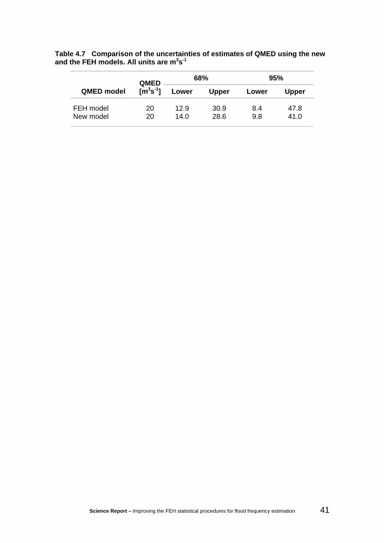
Science Report – Improving the FEH statistical procedures for flood frequency estimation 41
Table 4.7 Comparison of the uncertainties of estimates of QMED using the new and the FEH models. All units are m3s-1
68% 95%
QMED model QMED [m3s-1] Lower Upper Lower Upper
FEH model 20 12.9 30.9 8.4 47.8 New model 20 14.0 28.6 9.8 41.0

42 Science Report – Improving the FEH statistical procedures for flood frequency estimation
5 Use of donor sites When conducting a flood frequency analysis at an ungauged site, the FEH strongly recommends transferring data from catchments judged to be hydrologically similar to the target site but for which annual maximum flood data are available. However, in a comprehensive assessment of the FEH statistical method, Morris (2003) found inappropriate adjustment of QMED using donor and analogue catchments to be a major source of potential error. Morris’ study also identified regional patterns in the QMED residuals and suggested that considerations of on-line or off-line donors could potentially enhance the adjustment procedure. In a separate study, Kjeldsen and Jones (2007) analysed the benefits of using data transfer from donor sites from the perspective of reducing prediction variance at the site of interest. The results obtained by Kjeldsen and Jones (2007) enable a more analytical approach than that of Morris (2003) and the resulting improved data transfer scheme is presented below.
5.1 FEH donor adjustment Once a suitable donor site has been identified, the index flood at the site of interest is estimated as
cdsg
obsgcdssadjs QMED
QMEDQMEDQMED
,
,,, = , (5.1)
where subscript s refers to the ungauged target (or subject) site and g the gauged donor site, and the subscript cds refers to the estimates derived from catchment descriptors at the gauged and target sites, obs the observed value at the gauged site and adj the adjusted value at the target site. While this adjustment assumes the residuals from the QMED equation at both the target and the donor site exhibit the same behaviour, the recommended procedure makes no use of the distance-based relationship for the modelling-error correlation that is included in the FEH GLS-model.
5.2 New data transfer scheme A major advance from the FEH statistical method developed as part of this project is the ability to identify and estimate a separate model for the model error correlations (Kjeldsen and Jones, 2008). This is shown for the new QMED model in equation (4.15). Kjeldsen and Jones (2007) defined a revised data transfer scheme as an alternative to that suggested by the FEH study, which is introduced here as the “new data transfer scheme” and is given as
a
cdsg
obsgcdssadjs QMED
QMEDQMEDQMED ⎟
⎟⎠
⎞⎜⎜⎝
⎛=
,
,,, , (5.2)
where the new parameter a is estimated by minimising the prediction variance of (the logarithm of) QMEDs,adj, and is given by
ggsg h
ra+
= 2
2
,η
ηη σ
σ, (5.3)
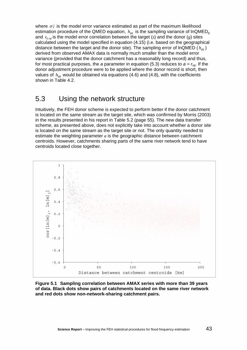
Science Report – Improving the FEH statistical procedures for flood frequency estimation 43
where 2ησ is the model error variance estimated as part of the maximum likelihood
estimation procedure of the QMED equation, ggh is the sampling variance of lnQMEDg and sgr ,η is the model error correlation between the target (s) and the donor (g) sites calculated using the model specified in equation (4.15) (i.e. based on the geographical distance between the target and the donor site). The sampling error of lnQMED ( ggh ) derived from observed AMAX data is normally much smaller than the model error variance (provided that the donor catchment has a reasonably long record) and thus, for most practical purposes, the a parameter in equation (5.3) reduces to a = rsg. If the donor adjustment procedure were to be applied where the donor record is short, then values of ggh would be obtained via equations (4.6) and (4.8), with the coefficients shown in Table 4.2.
5.3 Using the network structure Intuitively, the FEH donor scheme is expected to perform better if the donor catchment is located on the same stream as the target site, which was confirmed by Morris (2003) in the results presented in his report in Table 5.2 (page 55). The new data transfer scheme, as presented above, does not explicitly take into account whether a donor site is located on the same stream as the target site or not. The only quantity needed to estimate the weighting parameter a is the geographic distance between catchment centroids. However, catchments sharing parts of the same river network tend to have centroids located close together.
-0.6
-0.4
-0.2
0
0.2
0.4
0.6
0.8
1
0 50 100 150 200
cor[ln[m]i, ln[m]j]
Distance between catchment centroids [km]
Figure 5.1 Sampling correlation between AMAX series with more than 39 years of data. Black dots show pairs of catchments located on the same river network and red dots show non-network-sharing catchment pairs.

44 Science Report – Improving the FEH statistical procedures for flood frequency estimation
To further investigate the potential benefits of including information about the network structure, the sampling correlation between AMAX series at different sites was considered. Figure 5.1 shows the correlation between log-QMED at different sites with more than 39 years of overlapping records plotted against distance between catchment centroids.
The black dots indicate pairs of sites that are located on the same river network while the red dots indicate pairs that are not. Of course, there are far more red than black dots, but note that the black dots are mostly confined to the left side of the plot. This is because catchments sharing the same network are likely to be geographically close to each other. For the purpose of this project, it was not considered feasible to further investigate the potential for developing separate model error correlation models for the cases in which a donor is located either on the same river network as the subject site or not. However, the conclusion drawn from Figure 5.1 is that there is no clear difference in the patterns of correlation-against-distance for the two cases, and thus that the simple procedure outlined in Section 5.2 should be used in all cases.
5.4 Performance The effect of data transfer when predicting QMED for ungauged catchments has been investigated based on estimates of QMED obtained for each of the 602 catchments used in this study. The following four approaches to estimation of QMED were tested.
• Using only the regression model in equation (4.13) predicting QMED based on catchment descriptors only.
• Identifying the geographically closest (catchment centroids) out of the 601 other gauged catchments and using the new data transfer procedure in equation (5.2).
• Identifying the donor as above (i.e. the geographically closest catchment), but using the FEH data transfer procedure (equation 5.1).
• Identifying the closest of the 601 other gauged catchments in terms of hydrological similarity as defined by the FEH (i.e. using ln[AREA], ln[SAAR] and BFIHOST).
To assess the performance of each of the three data-transfer methods outlined above, the root mean square error (RMSE) was derived for each method as
( )5
lnln1
2,,,
−
−=∑=
M
QMEDQMEDRMSE
M
iigiadjs
, (5.4)
where the subscripts s, g and adj are described in a previous section. The degree of freedom is M-5 = 602 – 5 = 597 corresponding to the five regression parameters in the QMED model. The resulting RMSE values obtained for each of the three options are shown in Table 5.1, where it can be observed that, while the new data transfer method improves the RMSE when compared to using regression only, the FEH data transfer scheme has a higher RMSE than regression only. The latter finding indicates that, on average, the FEH data transfer scheme does not improve the prediction of QMED. The high RMSE value (0.475) obtained when using a donor site identified based on hydrological similarity clearly shows that this method is not performing well. In fact, it performs much worse than the regression model alone without any donor transfer.

Science Report – Improving the FEH statistical procedures for flood frequency estimation 45
Table 5.1 RMSE for each of the three methods predicting QMED in ungauged catchments.
Method RMSE Regression only, equation (4.13) 0.357 New data transfer 0.327 FEH data transfer: Geographically close 0.377 FEH data transfer: Hydrological similarity 0.475 To further investigate the structure of the RMSE values, the 602 catchments were divided into 20 groups according to the distance between a particular catchment and its closest donor catchment. Each of the 20 groups span a distance of 1 km and within each group the RMSE was estimated as
( )∑=
−=iM
jobsjjadjs
ii QMEDQMED
MRMSE
1
2,,, lnln1 , (5.5)
where Mi is the number of catchment pairs in the i’th group. For each of the first three methods in Table 5.1, the RMSE was estimated for each of the 20 groups and the results plotted on Figure 5.2.
0
0.1
0.2
0.3
0.4
0.5
0.6
0.7
0.8
0 5 10 15 20
RMSE
Distance between catchment centroids (km)
FEH Regression only
FEH data transfer
New data transfer
Figure 5.2 RMSE for 1 km intervals in distance between target and donor sites.
As observed on Figure 5.2, the RMSE derived using the regression model only is relatively independent of distance. Both the FEH and the new transfer scheme have improved the prediction of QMED compared to using a regression-only approach for very short distances less than 3 km. In general, the new transfer scheme consistently

46 Science Report – Improving the FEH statistical procedures for flood frequency estimation
performs better than both the regression-only option and the FEH data transfer scheme, whereas the FEH method often gives higher RMSE values than the regression model alone. This is confirmed by the average RMSE values reported in Table 5.1.
The FEH-related transfer methods included in Table 5.1 may not be considered immediately representative of the adjustments being made by practitioners since these often involve several catchments and a mixture of both “donors” (geographically close) and “analogues” (hydrologically similar) catchments. Given the scope for personal choice in selecting the contributing catchments, it would be impossible to construct an automatic procedure to represent this more closely. Nevertheless, the results here provide evidence that the use of “analogue” (hydrologically similar) catchments in the data transfer methodology is likely to make estimates of QMED worse, rather than better.
5.5 Discussion of data transfer The introduction in this study of a distance-based weighting scheme applied to the data transfer ratio is consistent with many of the recommendations made by Morris (2003) following a comprehensive review of the performance of the FEH statistical method. Firstly, the model in equation (4.15), describing the model error correlation as a function of geographical distance, is a direct consequence of the inability of a simple regression model using aggregated catchment descriptors to fully represent the hydrology of complex real catchments and to reflect the regional patterns in this inability. The only option for removing the model error is to improve the regression model by introducing improved catchment descriptors. Secondly, Morris (2003) suggested weighting the donor adjustment coefficients based on catchment similarity (as measured using ln[AREA], ln[SAAR] and BFIHOST). However, as shown in Table 5.1, a method where the weight is based on geographical distance (as in this study) should be the preferred option, rather than a method where the choice of donor is based on catchment similarity. Thirdly, it was suggested by Morris (2003) that consideration of whether the target and donor catchments are located on the same river network or not (on-line or off-line) could potentially help to reduce prediction errors further. While this effect has not been studied exhaustively here, the geographical distance between centroids for catchments located on the same river network is generally small, i.e. the weighting parameter derived from an on-line donor catchment is likely to be relatively high in the new transfer scheme. Further investigations would require scale considerations, such as questions as to whether data from a small unregulated tributary should be used to adjust QMED for a large regulated main river and vice versa.
5.6 Example: donor transfer In the example provided in Section 4.6.2, QMED was estimated at an ungauged site with grid coordinates (580550, 223300) and the resulting estimates of QMED with associated confidence intervals shown in Table 4.6. Here an example of the new donor transfer procedure is presented by considering a number of possible donor sites for the subject site. Figure 5.3 shows the location of the target site as well as the location of three on-line donors and four off-line donors selected based on the similarity to the subject site in terms of AREA, SAAR and BFIHOST.
Details of the subject catchment for this example and all the potential donor catchments are shown in Table 5.2.

Science Report – Improving the FEH statistical procedures for flood frequency estimation 47
SUBJECT
37016
37017
37010
37008
37020
0 2 4
km
SUBJECT
33057
SUBJECT
38004
Chelmsford
Cambridge
Colchester
0 5 10
km
River
Catchment Boundary
Gauging station
Figure 5.3 Location of target site and all potential donor sites.

Science Report – Improving the FEH statistical procedures for flood frequency estimation 48
Table 5.2 Relevant catchment descriptors (FEH CD-ROM V.2) for the subject site and the potential on- and off-line donor catchments.
National River Flow Archive (NRFA) No.
RIver Location Easting
(m)
Northing
(m)
AREA
(km2)
SAAR
(mm)
FARL
(-)
BFIHOST
(-) Subject 580550 223300 150.95 578 0.994 0.496 On-line donors 37016 Pant Copford Hall 566850 231400 63.77 588 0.997 0.404 37017 Blackwater Stisted 579250 224300 140.38 579 0.994 0.493 37010 Blackwater Appleford Bridge 584500 215800 247.09 572 0.992 0.477 Off-line donors 37008 Chelmer Springfield 571250 207050 189.65 584 0.985 0.492 37020 Chelmer Felsted 567100 219550 132.9 588 0.982 0.468 38004 Rib Wadesmill 536100 217350 136.65 625 0.999 0.469 33057 Ouzel Leighton Buzzard 491700 224050 122.39 643 0.991 0.524

Science Report – Improving the FEH statistical procedures for flood frequency estimation 49
Table 5.3 Estimation of QMED at the ungauged subject site using both: i) The FEH data transfer scheme – equation (5.1). ii) The new data transfer scheme – equation (5.2). NRFA No. River Location No. of
obs Sample
QMEDobs(m3/s)
Model QMEDcds
(m3/s)
Distance1 (km)
Weight2
a FEH
factorNew
factorFEH
QMEDadj3
(m3/s)
New QMEDadj
4
(m3/s) Subject 10.7 On-line donors 37016 Pant Copford Hall 38 8.9 7.1 15.9 0.33 1.26 1.08 13.4 11.5 37017 Blackwater Stisted 34 13.8 10.2 1.6 0.69 1.36 1.23 14.5 13.2 37010 Blackwater Appleford Bridge 41 11.3 16.5 8.5 0.40 0.69 0.86 7.3 9.2 Off-line donors 37008 Chelmer Springfield 37 14.8 13.1 18.7 0.32 1.13 1.04 12.0 11.1 37020 Chelmer Felsted 33 13.5 10.5 14.0 0.35 1.28 1.09 13.6 11.6 38004 Rib Wadesmill 44 12.1 13.8 44.8 0.19 0.88 0.98 9.4 10.4 33057 Ouzel Leighton Buzzard 22 7.6 11.2 88.9 0.08 0.68 0.97 7.2 10.3 Notes: 1 Distance between catchment centroids of subject site and donor catchment.
2 The weight a is defined as a = rsg. 3 Calculated using the FEH data transfer scheme equation (5.1). 4 Calculated using the new data transfer scheme equation (5.2).

50 Science Report – Improving the FEH statistical procedures for flood frequency estimation
Estimation of QMED at the subject site using the new data transfer scheme requires the calculation of the following quantities.
• Estimates of QMEDcds using catchment descriptors at both the subject and the target sites.
• An estimate of QMEDobs at the gauged donor site.
• The geographical distance (km) between the centroids of the subject and donor site.
Table 5.3 shows the calculation of the adjusted QMED values for each of the potential donor sites identified in Table 5.2 using both the new and the FEH data transfer methods. Note that the new data transfer method considers only a single donor site at the time.
On comparing the adjusted QMED values (QMEDadj) obtained using the two different methods, it is clear that the variation between the estimates is smaller for the new method than for the FEH method. This happens because the adjustments to the regression-only estimates are always smaller for the new adjustment method than for the FEH method. These adjustments are shown in Table 5.3 in the columns headed “FEH factor” and “New factor”. The “New factor” is the a’th power of the “FEH factor”, as shown by comparing equations (5.1) and (5.2).
In Table 5.3, one may note that the sample median for The Blackwater at Appleford Bridge is lower than the sample median for Stisted, even though the former is downstream of the latter. It might be thought that this could not be explained by attenuation effects related to flood plains between the two locations. The record lengths are different for the two catchments and this might be a partial explanation. However, examination of the HiFlows-UK records for these catchments indicates that the annual maximum flows for the same years are often such that those for the downstream catchment are lower than those for the upstream catchment, although not consistently. This may warrant further investigation.

Science Report – Improving the FEH statistical procedures for flood frequency estimation 51
6 Improving the FEH pooling procedure Use of the pooling-group method, as described by Robson and Reed (1999), was introduced in the FEH to overcome the problems often associated with the use of fixed regions such as those used in the FSR. These problems include issues of the regional memberships of catchments located on or near the boundary between two or more regions and the pooling of data that are geographically close but not necessarily similar in terms of hydrology.
A subsequent appraisal of the FEH statistical method carried out by Morris (2003) resulted in valuable feedback and highlighted a number of methodological issues in need of refinement and further research, including the following points.
• Poor performance of the pooling method for certain catchments when compared to at-site data.
• The weighting of L-moment ratios within pooling-groups depends on the rank, rather than directly on distance in catchment descriptor space. By default the rank is the ordering by distance in catchment descriptor space..
• Using a variable size of pooling-group depending on return period can lead to contradictory flood estimates.
In his appraisal, Morris (2003) found that a “single national growth factor performed better than the default FEH pooling-groups at the 10, 15 and 30-year return periods and almost as well at the 50-year (when tested at gauged locations, with the gauging station excluded from the pooling-group).”
Other issues regarding the suitability of the pooling-group heterogeneity measure (H2) and the procedure for adjusting the growth curve for the impact of urbanisation were also discussed by Morris (2003), but are outside the scope of this project. Some have already been addressed: for example, Bayliss et al. (2006) presented an improved method for the adjustment of FEH growth curves based on URBEXT2000 rather than URBEXT1990 as used in the FEH.
The FEH pooling-group method is a hybrid of the index-flood method (Stedinger et al., 1993) combined with the Region of Influence (ROI) approach for formation of pooling-group suggested by Burn (1990) on the basis of work by Acreman and Wiltshire (1987, 1989). The underlying assumption of the index-flood method is that the true distribution of the annual maximum peak flows from the different catchments in a pooling-group are identical, except for a scaling parameter denoted the index flood. By forming pooling-groups based on hydrological similarity, it is assumed that the catchment descriptors used in the distance measure can adequately explain the variability of the growth curves (L-moment ratios) between the catchments. However, by subsequently ordering the catchments within the pooling-group based on their rank (or distance), the method acknowledges that the catchments are in fact not similar, and hence the method departs from the underlying assumptions of the index-flood method. While these considerations might not affect the practical use of the method, they are important when developing the underlying statistical framework necessary for optimising the performance of the pooling-group method. The development of the method needs to consider the following aspects.
• Formation of pooling-groups.
• Weights within pooling-groups.

52 Science Report – Improving the FEH statistical procedures for flood frequency estimation
• Size of pooling-group.
• Performance of method.
These four aspects of the method are highly inter-dependent and ideally should be considered simultaneously. However, it was necessary to adopt a more sequential approach for practical reasons. Each of the first three aspects were analysed in turn and, once a decision was made, the next aspect was considered. While the reporting might give the impression of a straightforward process, in practice the analysis was very exploratory and each aspect was re-investigated several times to assess the effects of changes related to the other aspects.
6.1 Pooled frequency analysis The FEH recommends the three-parameter Generalised Logistic (GLO) distribution for flood frequency analysis in the UK. The quantile function or inverse of the cumulative distribution function for estimating the T-year event, xT, is given as
( )( ) ( )( ) TT zTTx 11111 ξκβξ
καξ κκ =⎥⎦
⎤⎢⎣⎡ −−+=−−+= −− , (6.1)
where ξ , α , and κ are GLO model parameters, T is the return period and zT is the growth curve at T defined by the square brackets in equation (6.1). The parameter estimation method used in this study is the method adopted by the FEH (Institute of Hydrology, 1999) and is a variant of the method of L-moments described by Hosking and Wallis (1997). Given a flow series from a particular gauging station with a series of n annual maximum peak flow values, the location parameter, ξ , is estimated by equating the distribution median to the sample median
( )nxxmedian ,,ˆ1 K=ξ , (6.2)
which is given more explicitly in equation (4.1).
Next, the shape parameter, κ , and the rescaled scale parameter, ξαβ = , are estimated as
( )( ) ( ) ,ˆsinˆˆ
ˆsinˆˆ
,ˆ
22
2
3
κπκπκκπκβ
κ
ttt
t
−+=
−= (6.3)
where t2 and t3 are the sample L-moment ratios L-CV and L-SKEW, respectively, as defined by Hosking and Wallis (1997).
When extending the at-site analysis to a pooled frequency analysis, the FEH uses the median-based index-flood method. This means that the T-year event is estimated as
PT
PT zx ξ= , (6.4)
which has a similar structure to the at-site case in equation (6.1), but the superscript P indicates that the factors are obtained from a pooled analysis. The pooled growth curve
PTz is estimated using information from M sites in the pooling-group that are deemed
sufficiently hydrologically similar to the catchment of interest. The parameters of the pooled growth curve are estimated by substituting the pooled L-moment ratios, Pt2 and
Pt3 , into equation (6.3). The pooled L-moment ratios themselves are calculated as the weighted average of the individual at-site L-moment ratios within the pooling-group.

Science Report – Improving the FEH statistical procedures for flood frequency estimation 53
Thus, for a pooling-group consisting of M catchments, the pooled L-moment ratios are given as
∑=
=M
iirir
pr tt
1,,ω (6.5)
where ir ,ω are the weights assigned to the i’th catchment for L-CV (r = 2) or L-SKEW (r = 3).
The FEH recommended a set of weights based on rank within the pooling-group and record length, and the same weights were used for both L-moment ratios. In the following, new sets of improved weights will be derived based on a statistical model for the underlying statistical structure of the pooling-groups.
6.2 Performance measure To assess the performance of alternative pooling procedures, the FEH developed a pooled uncertainty measure (PUM) defined as
( ) 21
1
1
2lnln
⎟⎟⎟⎟
⎠
⎞
⎜⎜⎜⎜
⎝
⎛−
=
∑
∑
=
=M
ii
M
i
pTTi
T
w
xxwPUM
ii
, (6.6)
where Tx is the at-site and PTx is the pooled T-year growth factor, and wi is the weight
assigned to the i’th catchment. The at-site values of the growth factor are obtained from a GLO distribution fitted by L-moments.
The rationale behind the PUM measure is that a good pooling method will, on average, produce growth curves that are close to the true growth curves for the site of interest where the true growth factor in this study is defined as the at-site growth factor. Two minor changes to the FEH-PUM measure have been adopted in this study. Firstly, the FEH considered only catchments with a record length exceeding 20 years whereas in this study no such censoring of the dataset was applied and all catchments were used. Secondly, the FEH defined the weights to be equal to record length. However, it was found that using record length gave too much weight to a few catchments with long record length. The present study has used a new set of weights were defined as
161 i
ii n
nw
+= , (6.7)
where ni is the record length. This has the effect of reducing the importance assigned to individual catchments with long records, while still giving average and long records more importance than very short records.
The weights in equation (6.7) were selected on the basis of simulation experiments which compared the between-site variation of at-site estimates of the growth curves with the sampling errors in these estimates for different record lengths. Some statistical theory indicates how these results can be used to derive an “optimal” weighting scheme. Somewhat different weights would notionally be required for the growth-curves (and hence for the PUM measure) for different return periods. The divisor “16” in equation (6.7) is a compromise that should be suitable for all return periods. Preference is given here to having simple, understandable weights rather than to an “optimality” that relies on an inadequate model.

54 Science Report – Improving the FEH statistical procedures for flood frequency estimation
6.3 Formation of pooling-groups As in the FEH, this study has adopted the ROI approach for creating pooling-groups tailored to each specific site of interest. By considering catchments which are similar to the site of interest (gauged or ungauged) with regard to a chosen set of catchment descriptors, it is assumed that these catchments are also ‘hydrologically similar’. The term ‘hydrologically similar’ means that a particular site does not violate the fundamental assumption of the index-flood method, i.e. that the AMAX flood series is generated from an underlying flood distribution with high order moments (L-CV and L-SKEW) equal to those at the subject site. The FEH adopted a similarity distance measure (SDM) to judge the similarity between catchment pairs. The catchment descriptors defining the SDM are called the pooling variables and the SDM itself is defined as
∑=
⎟⎟⎠
⎞⎜⎜⎝
⎛ −=
n
k k
kjkikij
xxSDM
1
2,,
σω , (6.8)
where xi,k is the k’th pooling variable at the i’th catchment, kω is the weight assigned to the k’th pooling variable, and kσ is the standard deviation between sites of the k’th catchment descriptor. Morris (2003) found that varying the weights in the FEH SDM had little effect on the overall performance of the pooling method.
6.3.1 Selecting variables for formation of pooling-groups
Linear regression models describing the L-moment ratios (L-CV and L-SKEW) as a function of catchment descriptors were used to identify potential combinations of catchment descriptors to be used in the formation of pooling-groups, i.e. to define hydrological similarity. A comprehensive search was conducted to identify the optimal combinations of catchment descriptors when using from one to ten different descriptors. Both log-transformed and non-transformed versions of the catchment descriptors were included in the search. The L-moment ratios themselves were not log-transformed in this experiment.
A similar investigation was conducted as part of the FEH development (Vol.3, §16.4.2) where it was found that 37.5 per cent and 8 per cent of the between catchment variation of L-CV and L-SKEW, respectively, could be explained using a regression model. These relatively low r2 values are in stark contrast to the 94 per cent of explained variance for the index flood (QMED) and might help to understand why discrepancies between at-site growth curves and the corresponding growth curves obtained using the pooling-group method can occur. For QMED, the descriptors AREA and SAAR have a strong explanatory power, while there are no such useful descriptors for L-CV or L-SKEW. This is partly because L-CV or L-SKEW are both standardised variables. The effects of sampling error are relatively greater for L-CV, L-SKEW and for at-site growth curves than for QMED.
The FEH based the formation of pooling-groups on three catchment descriptors (ln[AREA], ln[SAAR] and BFIHOST) which were selected on the basis of the preliminary regression analysis. It was noted that regression models using a larger number of descriptors performed only marginally better.
Possible catchment descriptors for L-CV
The FEH Vol.3 (16.4.2) found that 37.5 per cent of the variation in sample L-CV values could be explained by a log-linear regression model based on ln[AREA], ln[SAAR],

Science Report – Improving the FEH statistical procedures for flood frequency estimation 55
BFIHOST, ln[CVRI] and the seasonality vector (XFLOOD, YFLOOD). In this study, the optimal regression model based on four descriptors uses ln[AREA], ln[SAAR], FARL and 1-FPEXT. While the first two descriptors are consistently being selected in the optimal model, there is some suggestion that the log-transformed versions of FARL and 1-FPEXT might also be useful candidates. This suggests there may be some minor benefit in a fuller consideration of other non-linear transformations of these variables. Other potential descriptors selected are generally highly correlated with ln[SAAR] and have therefore not been selected. A minimum of 10 other variables were selected before BFIHOST, which contrasts strongly with the findings of the FEH.
Possible catchment descriptors for L-SKEW
The FEH Vol.3 (16.4.2) found that only 8 per cent of the variation in sample L-SKEW values could be explained by a log-linear regression model based on ln[AREA] and ln[NWET]. Clearly, the relationship between sample values of L-SKEW and the catchment descriptors is less significant than for L-CV. The optimal four-parameter regression model describing L-SKEW included: ln[AREA], ln[SAAR], 1-FPEXT and AREA (untransformed). The FARL descriptor did not appear to be strongly linked to L-SKEW. Furthermore, as for L-CV, BFIHOST also appears not to be a controlling factor for L-SKEW.
6.3.2 Final distance measure
The regression models selected for L-CV and L-SKEW share three catchment descriptors: ln[AREA], ln[SAAR] and 1-FPEXT. Based on the strong links between FARL and L-CV, it was decided to include FARL with the three other catchment descriptors in a single distance measure to be used to select a single pooling-group to be used for both L-moment ratios.
In the FEH, the weights assigned to each of the three catchment descriptors in the SDM measure was initially set to unity, but later the weight assigned to ln[AREA] was changed to 0.5 as this descriptor was found to exert “too large an influence on the final selection of site” (Institute of Hydrology, 1999) without further specifying the exact meaning of this. In this study, the weight assigned to each of the four catchment descriptors (ln[AREA], ln[SAAR], FARL and FPEXT) was investigated through an empirical procedure and was based on PUM values calculated from the data-set.
At this stage in the procedure, the set of weights used within each pooling-group to calculate the pooled L-moment ratios have not yet been defined. Instead, the L-moment ratio (either L-CV or L-SKEW) for each catchment is weighted according to its record length as shown in equation (6.7). The first step in the procedure is to set all four weights in the SDM to unity. Next, the weight assigned to the first catchment descriptor was set to vary between zero and ten (step 0.25). For each combination of weights, pooling-groups containing 17 catchments were formed for each of the 602 catchments and the resulting PUM calculated. Re-scaling of each of the trial set of weights was undertaken to ensure that the weights in the SDM measure sum up to four (the same as unity weights). Note that 17 catchments were used as a reasonable first guess of pooling-group size at this stage in the procedure.
Having identified an optimal, or near-optimal, value of the weight of ln[AREA], the weight of the second catchment descriptor, ln[SAAR], was set to vary between zero and ten, with unity weight on FARL and FPEXT but with the weight on ln[AREA] changed from unity to the optimal weight identified in the previous step. As before, the optimal weight of ln[SAAR] is noted, and the procedure then moves on to FARL and finally FPEXT. The results obtained from the procedure are illustrated in Figure 6.1. For

56 Science Report – Improving the FEH statistical procedures for flood frequency estimation
each catchment descriptor the final weight is set to the value that results in the minimum PUM value. It was found that only one run through the procedure was necessary to obtain a stable set of weights.
0.185
0.19
0.195
0.2
0.205
0.21
0.215
0 2 4 6 8 10 12
Weight
PUM
lnAREAlnSAARFARL1-FPEXT
Figure 6.1 PUM values for different combinations of weights in the SDM measure as determined by the empirical procedure. Note that the weights on the x-axis represent the unscaled weights.
The final unscaled weights are obtained from the analysis in Figure 6.1 and are as follows: ln[AREA] (7.0), ln[SAAR] (1.25), FARL (0.25) and FPEXT (0.50). For ln[AREA] the weights were relatively insensitive for values between 5 and 8, and finally a value of 7 was chosen. These weights were subsequently scaled to ensure that they sum to four and the final SDM measure is shown below:
.04.0
2.0
05.01.0
37.0lnln
5.028.1
lnln2.3
2
222
⎟⎟⎠
⎞⎜⎜⎝
⎛ −+
⎟⎟⎠
⎞⎜⎜⎝
⎛ −+⎟⎟
⎠
⎞⎜⎜⎝
⎛ −+⎟⎟
⎠
⎞⎜⎜⎝
⎛ −=
ji
jijijiij
FPEXTFPEXT
FARLFARLSAARSAARAREAAREASDM
(6.9) In Figure 6.1 it can be observed that the effect of leaving out any of the catchment descriptors (setting the weight to zero) results in a substantially higher value of PUM, except for FARL. This suggests that FARL is the least important catchment descriptor in the distance measure.
6.4 Weight of L-moments within pooling-groups A method for assigning weights to individual members of a pooling-group based on record length and rank was developed as part of the FEH statistical method. In a part of his study which concentrated mainly on the spatial coherence of the estimates obtained as part of an automated procedure, Morris (2003) identified the following problems with the FEH weighting scheme.
• It depends on rank.

Science Report – Improving the FEH statistical procedures for flood frequency estimation 57
• The weights do not diminish gradually to zero down the ranked list of catchments by the point at which they leave the pooling-group.
• Use of record length in the weights results in undesirably high weights being assigned to low ranking sites with relatively long records.
The study then went on to suggest replacing the rank-based FEH weights with a set based on a distance in catchment descriptor space between the site of interest and individual sites in the pooling-group.
When developing a revised weighting scheme in this project, a number of issues were considered. Firstly, the idea put forward by Morris (2003) that the weighting should depend on distance in catchment descriptor space has been adopted, but in a modified form. Secondly, the revised weighting scheme makes a distinction between pooling-groups for gauged and ungauged sites. Where the existing FEH weighting scheme can only include the available at-site data by assigning the first rank position to the site of interest, the new methodology assigns relatively more importance to at-site data than data from other catchments in the pooling-group. Finally, a new set of weights is developed separately for L-CV and L-SKEW, although only one pooling-group will be created for each site of interest.
In Section 6.4.1 the structure of the new weighting scheme is outlined and the associated parameters for use with the weighting scheme will be estimated in Section 6.4.2. The statistical model forming the basis of the weighting scheme is described in detail in Appendix D.
6.4.1 New weighting scheme
Based on the discussion above and in Appendix D, the suggested form of the weighting for a particular L-moment ratio was defined as
( )( ) 1−++∝ βiii SDMfcαω , i = 1,…, M, (6.10)
where ci is the sampling variance of the L-moment ratio for the i’th site , M is the total number of sites in the pooling-group and SDMi is the distance in catchment descriptor space between the subject site and the i’th site (specifically this is the similarity distance measure (SDM) of Section 6.3).
The sum ( )βiSDMf+α in equation (6.10) represents the variance of the structural error. This error represents the uncertainty arising because the true values of the L-moment ratios for each site in the pooling-group are different from the corresponding true value at the subject site. There is an assumption that these differences tend to grow with an increase in the distance in the catchment property space ( iSDM ) between the subject catchment and the i’th catchment and this is the role of the term f in the sum. The vector β contains a set of model parameters for f that need to be estimated.
It is necessary to distinguish the roles of α and f within the model, which can be done by imposing the constraint that ( ) 00 =βf . This means that the term α represents the effect of differences between the true L-moment ratios for catchments at a distance of zero in catchment descriptor space ( 0=iSDM ). That is, if two catchments had exactly the same values for the four catchment descriptors defining SDM, they would still not be expected to have exactly the same true underlying values for their L-moment ratios. Next, the term f represents the effect of the extra difference to be expected for more dissimilar catchments (i.e. larger SDM values). When catchments in the pooling-group become increasingly different from the subject catchment (as measured by the catchment properties), the values of f will become larger and the weights determined

58 Science Report – Improving the FEH statistical procedures for flood frequency estimation
from equation (6.10) will be smaller. Correspondingly, if the record length available at a catchment in the pooling-group is relatively short, then the sampling variance of the L-moment ratios, ic , will be relatively large and hence the weight will be small.
Both the functional form of f and its associated parameter vector β need to be estimated based on analysis of the observed data, which is reported in Section 6.4.2, and this also leads to the estimation of α . For convenience, the following notation is defined for use in the weighting scheme:
( )βii SDMfb +=α . (6.11)
Before estimating the model parameters, the structure of the new weighting scheme is introduced. The weight assigned to each site in the pooling-group depends on whether the subject site is gauged or ungauged. The two cases are presented separately.
No information at subject catchment (ungauged)
The weighted average L-moment ratio is calculated as
∑=
=M
iirir
pr tt
1,,ω (6.12)
for a set of weights ir ,ω which sum up to one, and where tr,i is the L-CV (r = 2) or L-SKEW (r = 3) for the i’th catchment in the pooling-group. For the ungauged catchment, the weights are defined as
{ }{ }∑
=
−
−
+
+= M
kkk
jjj
bc
bc
1
1
1
ω , (6.13)
where different sets of coefficients jc and jb for the two L-moment ratios give two different sets of weights jω .
Estimation of the model parameters is outlined in Section 6.4.2.
Data available at the subject catchment (gauged)
When data are available at the subject catchment it is considered in the form of an observed value of the L-moment ratio, tr, which has a sampling error variance as a result of being estimated from a data series of limited extent. As for the ungauged case, the weighted average L-moment ratios are calculated as
∑=
=M
iirir
pr tt
1,,ω , (6.14)
using a set of weights ir ,ω which sum up to one, and where tr,i is the L-CV (r = 2) or L-SKEW (r = 3) for the i’th catchment in the pooling-group. As the observed data at the subject catchment are considered more important than information at other catchments in the pooling-group, a set of weights have been defined reflecting this distinction. Thus the weights are
Science Report – Improving the FEH statistical procedures for flood frequency estimation 59
{ }{ }∑
=
−
−
+
++
+= M
kkk bc
bccbc
b
1
1
2111
11
11ω , (6.15a)
{ } { }{ }
Mjbc
bcbccM
kkk
jjj ,,2
1
1
11111 L=
+
++=
∑=
−
−−
ω , (6.15b)
where it is assumed that the subject catchment has subscript 1 in the list of catchments in the pooling-group.
The actual model parameters, which are used for both the gauged and ungauged cases, are estimated in Section 6.4.2. Specifically, these areα and β , which determine
jb via equation (6.11). The other quantities jc are the sampling variance of the L-moment ratios and are specified in Section 6.4.2 via equations (6.18) and (6.19).
6.4.2 Estimation of model parameters An initial attempt to estimate the parameter α and a linear form of the function f in equation (6.11) by minimising the PUM score was unsuccessful due to the relative insensitivity of the PUM scores to those model parameters. As an alternative, the parameters were estimated based on a variogram analysis. The linkage between the weights and the variogram is complex and derived through consideration of the structure of the statistical errors involved in the estimation of the pooled L-moment ratios: see Appendix D. The key-result is that the points in a sample variogram, γ , should cluster around a line defined as
( ) ( )βαγ sfs += 2 , (6.16)
where raw estimates of this function can be obtained for distances s = SDMij, and where SDMij, is the distance in catchment descriptor space between catchments i and j as defined in equation (6.9) (for a complete description please refer to Appendix D). By noting the similarity between the function defining the weights in equations (6.11) and (6.16) above, it is possible to derive a set of weights for both L-CV and L-SKEW based on a set of models fitted to sample variograms of the L-CV and L-SKEW sample values. Equation (6.16) represents the theoretical variogram of the true L-moment ratios. A raw estimate of the variogram would be affected by terms related to the variogram of the sampling errors and a correction is therefore necessary. In addition, sampling errors in the raw estimates are reduced by averaging over a number of pairs of catchments that are approximately the same distance apart. The corrected and smoothed variogram estimator is given, for r = 2,3, by
( ) ( ) ( ) { }( )∑Δ ⎪⎭
⎪⎬⎫
⎪⎩
⎪⎨⎧
⎟⎟⎠
⎞⎜⎜⎝
⎛−+−−
Δ=
ssnjrirji
ji
ijjijrirr ttcc
nnncctt
ssns
,,,
2,, ,cor2
,1γ̂ , (6.17)
where the set ( )ssn Δ, consists of the catchment pairs (i,j) for which the distance SDMi j is between s-½Δs and s+½Δs, ic is the sample variance of the r’th L-moment ratio (tr,i) for catchment i which has record length in , and ijn is the number of overlapping years between catchments i and j. Here the distance SDMi j is measured in catchment descriptor space using equation (6.9). The notation ( )ssn Δ, denotes the number of pairs in the set ( )ssn Δ, .

60 Science Report – Improving the FEH statistical procedures for flood frequency estimation
The sampling variance, jc , of the higher order L-moment ratios can be estimated using different methods. Kjeldsen and Jones (2004) developed a set of approximate analytical estimators, but they were considered too complex to be of practical use in this study, especially as part of the weighting scheme in equations (6.12) to (6.15). As an alternative, a set of simple approximations were developed based on Monte Carlo simulations from a “typical” GLO distribution, selected as representative of the whole of the UK. This study related the sampling variance of L-CV and of L-SKEW to record length only, and gave the following results:
L-CV 1
02609.0−
=k
k nc (6.18)
L-SKEW 2
2743.0−
=k
k nc (6.19)
Notionally, these sampling variances should vary with the parameters of the distribution appropriate for any given site, but the use of the “average” values should be adequate for the purpose of defining the weights used to calculate the estimated L-moment ratio for a pooling-group.
The correlation of the sample L-moment ratios between sites was obtained through a bootstrapping experiment and defined as a function of geographical distance between catchment centroids:
L-CV { } ( )ijji dttcor 030.0exp, ,2,2 −= (6.20a)
L-SKEW { } ( )ijji dttcor 050.0exp, ,3,3 −= (6.20b)
where ijd is distance between catchment centroids in kilometres. The structure of the bootstrapping experiment was similar to that used in Section 4.3 for estimating the correlation of the log-transformed QMED values between sites.
Information concerning typical distances in catchment descriptor space observed in a pooling-group is required in order to define appropriate values of s=SDM and the total number of bins for which the variogram is defined. Table 6.1 shows the average and maximum distance observed when a pooling-group consisting of 30 catchments was defined for each of the 602 catchments used in this study.
Table 6.1 Typical values for distances in catchment descriptor space observed for 602 pooling-groups consisting of 30 catchments each.
Distance Average distance within pooling-groups 0.64 Average maximum distance within pooling-groups 0.85 Maximum average distance within pooling-groups 3.46 Maximum observed distance between any two catchments 11.04 Based on the distances in Table 6.1, it was decided that the maximum distance within any pooling-group would usually be below 4.0. Based on a number of trials, the number of distance-intervals, the number of different ),( ssn Δ sets, was set to 100. Estimates of the variograms for L-CV and L-SKEW obtained using equation (6.17) are shown in Figure 6.2. The shape of the plots indicated that a functional relationship could be fitted, linking the variogram to the distance, using an empirical type function that was found to fit the data reasonably well:

Science Report – Improving the FEH statistical procedures for flood frequency estimation 61
( ) ( )δ
βββγ ⎟
⎟⎠
⎞⎜⎜⎝
⎛⎥⎦
⎤⎢⎣
⎡−−+=
321 exp1 sss (6.21)
where ( )321 ,, βββ=Tβ are model parameters and δ is a binary parameter that can be either 1 or 0, depending on whether the variogram has a nugget at distance zero (δ =0) or not (δ =1) . When using equation (6.21) for defining the parameters in equation (6.11), it should be noted that if a nugget exists then 22 βα = .
0
0.002
0.004
0.006
0.008
0.01
0.012
0.014
0 1 2 3 4 5
Distance (SDM)
γ(SD
M)
-0.015-0.01
-0.0050
0.0050.01
0.0150.02
0.0250.03
0 1 2 3 4 5
Distance (SDM)
γ(SD
M)
Figure 6.2 Variograms for L-CV (top) and L-SKEW (bottom) plotted as a function of distance in catchment descriptor space. Maximum distance is set to 4 and subdivided into 100 intervals.
Table 6.2 Model parameters for variograms as defined in Equation (6.21)
Model parameter L-CV L-SKEW
1β 0.0047 0.000
2β 0.0023 0.0219
3β n/a 0.2360
δ 0 1

62 Science Report – Improving the FEH statistical procedures for flood frequency estimation
The three parameters ( )321 ,, βββ controlling the variograms were estimated based on a least squares analysis. The resulting model parameters are shown in Table 6.2.
In terms of the weighting of the L-moment ratios within each pooling-group, the weighting parameters bj for L-CV and L-SKEW are defined as
L_CV ⎟⎠⎞
⎜⎝⎛ +=
20023.00047.0 jj SDMb (6.22a)
L-SKEW ⎟⎟⎠
⎞⎜⎜⎝
⎛⎥⎦
⎤⎢⎣
⎡−−=
2360.0exp10219.0 j
j
SDMb (6.22b)
where SDMj is the distance in catchment descriptor space from the subject site to the j’th site in the pooling-group. Note that while a nugget effect was observed in the sample variogram for L-CV, no such effect was detected for L-SKEW.
Equations (6.22a and b) are combined with the equations (6.18-9) to give the weights in the two cases of gauged or ungauged catchments (equations (6.13) and (6.15)), from which the pooled L-moment ratios can be derived through equation (6.5).
The variogram functions and the weighting scheme derived from them are considered fairly reliable in terms of stability across other choices that might have been made concerning the functional form of the variogram (including the decision whether to have a nugget effect or not), and also in terms of the range of distances over which the function is fitted. Appendix D outlines the relation between the variogram and the weights Examination of this will show that this link might be regarded as somewhat tenuous. The context here is that we are seeking to respond to FEH-users’ comments that the weights given to catchments in a pooling-group procedure should be related to the measure of hydrological similarity between catchments (SDM here). The present analysis has used the available data to suggest both what form this relationship should take and to what extent the weights should vary with SDM. The variation of the weights is illustrated later in Section 6.7.
6.5 Size of pooling-groups The final step in the development of the pooling procedure is to determine the number of catchments to be included in a pooling-group. The best size of a pooling-group is a trade-off between the bias (precision) and variance (uncertainty) of the estimated T-year flow. Too many sites in a pooling-group will increase the possibility of including sites that are markedly different from the target site, thereby increasing the bias of the T-year event. On the other hand, including too few sites will lead to estimates with a larger variance (higher uncertainty) for the T-year estimate than necessary. Based on a series of Monte Carlo experiments, Hosking and Wallis (1997) found that little could be gained, in terms of RMSE, by using regions larger than about 20 sites.
Within the context of a pooling-group procedure such as that recommended in the FEH, the size of the pooling-group used has implications for the amount of effort that would need to be expended by a “User”, since the records for catchments in the pooling-group should be brought up to date and checked. Fortunately, the size of pooling-groups that appear to be best on other grounds do not seem to lead to too onerous a task for the user.
The size of a pooling-group can be quantified either in terms of the number of sites or the total number of AMAX events. The FEH opted for the latter measure because of the large variation in record length observed in practice. While not eradicated, this problem

Science Report – Improving the FEH statistical procedures for flood frequency estimation 63
might be less severe when using the updated HiFlows-UK dataset where the average record length is approximately 10 years longer than the original FEH data set.
The FEH introduced a 5T rule, allowing the size of the pooling-group to be determined by the target return period. For example, for a target return period of T = 100 years, sites should be added to the pooling-group until 500 AMAX events has been reached. However, the FEH stated that this was indeed a ‘rule-of-thumb’, and based on intuition rather than the outcome of a particular analysis. Later, Morris (2003) found that varying pooling-group size according to the 5T rule could lead to contradictory flood estimates and cites an example where a 200-year flood is estimated as being smaller that the 10-year flood. As a result, Morris (2003) recommended using a single pooling-group size for all return periods, and used a total number of AMAX events corresponding to a 200-year target return period, i.e. 1,000 AMAX events.
In this study, the size of the pooling-group was investigated in terms of both the number of catchments and the number of AMAX events. In each case the PUM criterion (equation (6.6)) was used to assess the appropriate size. Figure 6.3 shows how the PUM criterion varies according to size for both cases.
00.050.1
0.150.2
0.250.3
0.350.4
0 200 400 600 800 1000
No. AMAX events in pooling group
PUM
T=100
T=50
T=20
00.050.1
0.150.2
0.250.3
0.350.4
0 5 10 15 20 25 30 35
No. sites in pooling group
PUM
T=100
T=50
T=20
Figure 6.3 PUM as a function of pooling-group size measured by a) number of AMAX events and b) number of sites. PUM was calculated for both T=20, T=50, and T=100.

64 Science Report – Improving the FEH statistical procedures for flood frequency estimation
For both measures of pooling-group size, the PUM decreases rapidly from high values for very small pooling-groups until a size of 10 sites (or about 300 AMAX events) is reached. Between 10 and 17 sites (or between 300 and 500 AMAX events) little change in PUM can be observed. After this point the PUM rises slowly for increasing pooling-group size. There is no evidence from the data analysed in this study that the pattern described above changes as a function of target return period. Based on these results, there seems to be no reason why one method of measuring pooling-group size should be preferred over another. It is therefore recommended that the current measure used in the FEH be retained, that is, to go on using the number of AMAX events.
With regard to the actual size of the pooling-groups, the current FEH practice recommends using the 5T rule, but the results reported here support the recommendation made by Morris (2003) that a single pooling-group size should be applied irrespective of the target return period. The results shown in Figure 6.3 suggest little effect on the PUM measure if pooling-groups are based on between 300 and 500 AMAX events. Consequently, using a default pooling-group size of 500 AMAX events is recommended for all return periods, which corresponds to the size of a pooling-group for a 100-year target return period under the current FEH guidelines.
6.6 Performance of pooling-groups The performance of the pooling-group method needs to be assessed for two different cases. Firstly, performance is assessed for the case of the ungauged site where no at-site data are available, and, secondly, for the gauged site, where the performance should be compared to the results obtained from a standard single-site flood frequency analysis. The methods used for assessing the two cases are very different and will be reported separately in the following.
6.6.1 The ungauged site
The pooling-group method derived in the previous sections is only one candidate out of many possible procedures that could have been specified. At each step in the development a range of different options could have been selected, which would have led to a modified end-product. However, the development should be reasonably close to an optimal procedure (with regards to PUM), as each step in the development was justified through careful analysis of the data. To provide further evidence of the improvements made during this project, the new method developed here is compared to the following series of alternatives.
• A simplified procedure (simple weights).
• A single UK growth factor.
• Pooling-groups based on geographical distance only.
• The FEH methodology.
• Weighted Least Squares (WLS) regression models for L-CV and L-SKEW.
Here the simple weights are defined using equation (6.7). The single UK growth factor is obtained by using the weighted average L-moment ratios, averaged for the whole of the UK. For the final option listed, the regression models are the models for L-CV and L-SKEW that are reported in Section 6.3.1, where they are used to help select the descriptors to be used in measuring the similarity between catchment: a weighted least squares (WLS) fit is used.

Science Report – Improving the FEH statistical procedures for flood frequency estimation 65
Table 6.3 Comparison of pooling methods using PUM.
T = 20 T = 50 T = 100 1 New method 0.1875 0.2576 0.3134 2 New method, simple weights 0.1886 0.2591 0.3152 3 Single UK growth curve 0.2164 0.2914 0.3501 4 Geographical proximity1 0.1926 0.2651 0.3226 5 FEH method2 0.1986 0.2718 0.3296 6 Regression models 0.1881 0.2598 0.3170 7 New method, gauged site 0.1095 0.1622 0.2062 Notes: 1Pooling-group size of 700 AMAX events. 2Pooling-group size of 500 AMAX events.
Each of the alternatives listed above has been assessed using the PUM measure by considering each of the 602 catchments, in turn, to be ungauged (i.e. the subject site is excluded from its own pooling-group), and calculating PUM for return periods of 20, 50 and 100 years. The results are summarised in Table 6.3. From this table, it is clear that the new method performs better than the existing FEH methodology. The FEH methodology included i) defining pooling-groups based on hydrological similarity as defined in the FEH (ln[AREA], ln[SAAR] and BFIHOST), and ii) calculating the weight of the individual L-moment ratios using the FEH weighting scheme (i.e. based on rank and record length). However, the analysis was based on the 602 AMAX series from HiFlows-UK data used in this study rather than the FEH dataset.
It is worth noting that the increase in performance gained by introducing the new weighting scheme is rather small compared to the method using relatively simple weights given by equation (6.7). However, the more complicated new weighting scheme is recommended as it includes an effect whereby the weights given to catchments in the pooling-group tend to decrease as the catchments become less hydrologically-similar to the subject catchment. This has previously been considered an important requirement by users commenting on the existing FEH pooling-group scheme.
The regression approach also produces competitive results. In fact, there is still some scope for improvement here since a full consideration of alternative transformations of the descriptors has not been undertaken -- specifically, the type of consideration reported in Section 4.4.3 for the QMED regressions, which led to an improved predictor of QMED.
Implementation of a regression-based approach would replace the pooling-group approach to estimating L-CV and L-SKEW with simple equations for these. There would be the possibility of extending these by adding a donor-catchment adjustment similar to that for QMED. Even if the regression approach could be improved, there is a good reason to retain the pooling-group approach in preference to it. Specifically, the pooling-group approach allows the User to incorporate up-to-date information from relevant sites without having to carry out a full investigation of all sites in the country.
6.6.2 The gauged site
At the gauged site the benefit of using pooled analysis should be compared to a direct at-site analysis of the available data, and should ideally consider aspects of variability and bias of the estimated design events. Based on a series of Monte Carlo experiments, Hosking and Wallis (1997) concluded that while pooled (or regional) analysis might be considered beneficial for a region overall, at-site analysis might still

66 Science Report – Improving the FEH statistical procedures for flood frequency estimation
be preferable at individual sites. The design of a suitable Monte Carlo experiment considering the whole of the UK was considered outside the scope of the current project. Instead, a more direct comparison was made based on the PUM criterion.
It can be argued that the PUM criterion is not suitable for a comparison of at-site and pooling procedures in the “gauged case”, as it will favour any pooling procedure giving results close to the at-site results without consideration of variability of the estimates. In particular, if a free choice of procedures were allowed, the PUM criterion would favour using only the at-site record. On the other hand, use of the PUM measure will allow a comparison between pooled analysis at a gauged and an ungauged site: the results provide a direct measure of the changes in the estimates due to the gauged-case weighting scheme introduced in this study. Furthermore, if the T-year estimates obtained through pooled analysis can be considered to have a lower variance than the corresponding at-site estimates, as shown by (for example) Kjeldsen and Jones (2006), then the PUM measure will reflect a practical consideration that the pooled estimates should not diverge too much from the at-site estimates in order to remain believable. The PUM values for the gauged case (weights calculated using equation (6.15)) are included as the bottom row of Table 6.3; the PUM values here are lower than the corresponding values at the ungauged site, indicating a closer correspondence to the at-site estimates.
6.7 Example: a pooling-group The application of the new pooling procedure for both a gauged and an ungauged subject is illustrated using catchment 37017 (Blackwater at Stisted) as an example. The gauging station (37017) is located at the grid reference (5678, 2324) where the FEH CD-ROM version 2.0 gives the following relevant catchment descriptors:
AREA = 140.38 km2 SAAR = 579 mm FARL = 0.994 FPEXT = 0.0688
Figure 6.4 AMAX events for gauging station 37017 (from HiFlows-UK).

Science Report – Improving the FEH statistical procedures for flood frequency estimation 67
The AMAX record consists of 34 observations classified as ‘suitable for pooling’ by HiFlows-UK, and the time series is shown in Figure 6.4.
This example will consider the two cases where a pooling-group is created for a gauged catchment and for an ungauged catchment.
6.7.1 Selection of the pooling-group
As the pooling-group for a gauged catchment will include the gauged record itself, and the total number of AMAX events in a pooling-group must exceed 500, the pooling-groups created for the two cases (gauged and ungauged) are slightly different and shown in Tables 6.4 and 6.5, respectively.
Both pooling-groups are created by searching through the database of 602 gauged catchments, identifying the catchments most hydrologically similar as defined by the standard distance measure (SDM) presented in equation (6.9).
6.7.2 Review of the pooling-group
The FEH suggests that an initial pooling-group should be reviewed and, possibly, adapted. In particular, the review should consider the following factors.
• Catchment location and period of AMAX record.
• Similarity in terms of flood seasonality.
• Similarity in terms of further catchment descriptors.
• Standard comments, and other information, about catchments and their AMAX records.
• Known special features of the subject catchment.
Because the FEH derives the weights of the L-moment ratios within a pooling-group based on both ranking and record length, it is recommended that, following a review, a pooling-group can be adapted by changing the relative ranking of the catchments, or by removing or adding catchments to the initial pooling-group (or possibly both).
In the new method the weights within a pooling-group are based on record length and distance from subject site in catchment descriptor space. Therefore, the relative ranking of the catchments within a pooling-group has no influence on the weights, and the only method for adapting a pooling-group is to remove or to add individual catchments.
The FEH recommends that only catchments that can be considered ‘rural’ should be included in the pooling-group, and that for an urban subject site, any adjustment should be made after the derivation of the ‘as-rural’ growth curve. Bayliss et al. (2006) updated the FEH urban-adjustment procedure to use the URBEXT2000 rather than URBEXT1990.

68 Science Report – Improving the FEH statistical procedures for flood frequency estimation
Table 6.4 Pooling-group for catchment 37017 (gauged)
j Site No. obs. AREA
[km2]
SAAR
[mm]
FARL
[-]
1-FPEXT
[-]
SDM
1 37017 34 140.38 579 0.994 0.9312 0.0000 2 37020 33 132.96 588 0.982 0.9341 0.1159 3 36005 39 155.85 580 0.994 0.9236 0.1690 4 33051 34 140.09 599 0.993 0.9482 0.2010 5 38004 44 136.69 625 0.999 0.9462 0.2277 6 33018 39 132.65 661 0.986 0.9373 0.2785 7 35008 37 126.98 577 0.996 0.9012 0.3638 8 34003 44 161.41 669 0.974 0.9149 0.4044 9 30005 35 123.50 646 0.973 0.9075 0.4046 10 33055 27 101.80 579 0.999 0.9386 0.4577 11 20003 41 162.76 724 0.987 0.9548 0.5447 12 39037 31 136.48 772 1.000 0.9237 0.5588 13 21027 29 155.39 774 0.997 0.9300 0.5731 14 54106 17 185.16 677 0.993 0.9583 0.5752 15 33012 43 137.99 585 0.992 0.8793 0.5812 Total 527
Table 6.5 Pooling-group for catchment 37017 (ungauged)
j Site No. obs. AREA [km2]
SAAR [mm]
FARL [-]
1-FPEXT [-]
SDM
1 37020 33 132.96 588 0.982 0.9341 0.1159 2 36005 39 155.85 580 0.994 0.9236 0.1690 3 33051 34 140.09 599 0.993 0.9482 0.2010 4 38004 44 136.69 625 0.999 0.9462 0.2277 5 33018 39 132.65 661 0.986 0.9373 0.2785 6 35008 37 126.98 577 0.996 0.9012 0.3638 7 34003 44 161.41 669 0.974 0.9149 0.4044 8 30005 35 123.50 646 0.973 0.9075 0.4046 9 33055 27 101.80 579 0.999 0.9386 0.4577 10 20003 41 162.76 724 0.987 0.9548 0.5447 11 39037 31 136.48 772 1.000 0.9237 0.5588 12 21027 29 155.39 774 0.997 0.9300 0.5731 13 54106 17 185.16 677 0.993 0.9583 0.5752 14 33012 43 137.99 585 0.992 0.8793 0.5812 15 54018 41 173.10 757 0.991 0.9244 0.5952 Total 534
The improved method for pooled frequency analysis derived in this study has retained the recommendation to use only rural catchments in the pooling-group, though the threshold for definition of ‘rural’ has changed following the adoption of URBEXT2000 rather than URBEXT1990. Where the FEH defined rural as catchments with URBEXT1990 values less than 0.025, this study defines rural as catchments with URBEXT2000 values less than 0.030 (Bayliss et al. ,2006) See also Section 2.1.1.

Science Report – Improving the FEH statistical procedures for flood frequency estimation 69
Table 6.6 Calculation of pooled L-moment ratios for 37017 (gauged)
L-CV L-SKEW
j Site No. obs.
SDM bj cj (bj + cj)-1 wj L-CV bj cj (bj + cj)-1 wj L-SKEW
1 37017 34 0.0000 0.00115 0.00079 515.30 0.6526 0.2232 0.00000 0.00857 116.66 0.1690 -0.0910 2 37020 33 0.1159 0.00275 0.00082 280.46 0.0327 0.2062 0.00850 0.00885 57.64 0.0835 -0.2121 3 36005 39 0.1690 0.00308 0.00069 265.32 0.0309 0.3074 0.01120 0.00741 53.72 0.0778 0.1389 4 33051 34 0.2010 0.00326 0.00079 247.06 0.0288 0.2403 0.01255 0.00857 47.34 0.0686 -0.1358 5 38004 44 0.2277 0.00339 0.00061 250.03 0.0291 0.3050 0.01356 0.00653 49.78 0.0721 0.1621 6 33018 39 0.2785 0.00363 0.00069 231.65 0.0270 0.2633 0.01517 0.00741 44.28 0.0642 0.2481 7 35008 37 0.3638 0.00398 0.00072 212.33 0.0247 0.3174 0.01721 0.00784 39.92 0.0578 0.0979 8 34003 44 0.4044 0.00414 0.00061 210.73 0.0246 0.2953 0.01795 0.00653 40.84 0.0592 0.2420 9 30005 35 0.4046 0.00414 0.00077 203.79 0.0237 0.2881 0.01796 0.00831 38.07 0.0552 0.0937 10 33055 27 0.4577 0.00433 0.00100 187.50 0.0218 0.3455 0.01875 0.01097 33.64 0.0487 0.3105 11 20003 41 0.5447 0.00462 0.00065 189.71 0.0221 0.4042 0.01972 0.00703 37.38 0.0542 0.2200 12 39037 31 0.5588 0.00466 0.00087 180.73 0.0211 0.4243 0.01985 0.00946 34.12 0.0494 0.3945 13 21027 29 0.5731 0.00471 0.00093 177.31 0.0207 0.3271 0.01997 0.01016 33.19 0.0481 0.2429 14 54106 17 0.5752 0.00471 0.00163 157.60 0.0184 0.3482 0.01999 0.01829 26.13 0.0379 0.3741 15 33012 43 0.5812 0.00473 0.00062 186.76 0.0218 0.2799 0.02003 0.00669 37.42 0.0542 0.0729 Total = 527 0.2514 0.0976

Science Report – Improving the FEH statistical procedures for flood frequency estimation 70
Table 6.7 Calculation of pooled L-moment ratios for 37017 (ungauged)
L-CV L-SKEW
j Site No. obs.
SDM bj cj (bj + cj)-1 wj L-CV bj cj (bj + cj)-1 wj L-SKEW
1 37020 33 0.1159 0.00275 0.00082 280.47 0.0886 0.2062 0.00850 0.00885 57.65 0.0945 -0.2121 2 36005 39 0.1690 0.00308 0.00069 265.34 0.0838 0.3074 0.01120 0.00741 53.73 0.0880 0.1389 3 33051 34 0.2010 0.00326 0.00079 247.05 0.0781 0.2403 0.01256 0.00857 47.33 0.0776 -0.1358 4 38004 44 0.2277 0.00339 0.00061 250.03 0.0790 0.3050 0.01356 0.00653 49.79 0.0816 0.1621 5 33018 39 0.2785 0.00363 0.00069 231.65 0.0732 0.2633 0.01517 0.00741 44.28 0.0726 0.2481 6 35008 37 0.3638 0.00398 0.00072 212.33 0.0671 0.3174 0.01721 0.00784 39.92 0.0654 0.0979 7 34003 44 0.4044 0.00414 0.00061 210.72 0.0666 0.2953 0.01795 0.00653 40.84 0.0669 0.2420 8 30005 35 0.4046 0.00414 0.00077 203.79 0.0644 0.2881 0.01796 0.00831 38.07 0.0624 0.0937 9 33055 27 0.4577 0.00433 0.00100 187.51 0.0592 0.3455 0.01875 0.01097 33.64 0.0551 0.3105 10 20003 41 0.5447 0.00462 0.00065 189.72 0.0599 0.4042 0.01972 0.00703 37.38 0.0612 0.2200 11 39037 31 0.5588 0.00466 0.00087 180.73 0.0571 0.4243 0.01985 0.00946 34.12 0.0559 0.3945 12 21027 29 0.5731 0.00471 0.00093 177.31 0.0560 0.3271 0.01997 0.01016 33.19 0.0544 0.2429 13 54106 17 0.5752 0.00471 0.00163 157.60 0.0498 0.3482 0.01999 0.01829 26.13 0.0428 0.3741 14 33012 43 0.5812 0.00473 0.00062 186.77 0.0590 0.2799 0.02003 0.00669 37.42 0.0613 0.0729 15 54018 41 0.5952 0.00478 0.00065 184.22 0.0582 0.1546 0.02014 0.00703 36.80 0.0603 0.1323 Total = 534 0.2958 0.1357

Science Report – Improving the FEH statistical procedures for flood frequency estimation 71
6.7.3 Deriving the pooling-group estimates
For the new pooling procedure developed in this study, the weights assigned to the individual values of L-CV and L-SKEW within a particular pooling-group are conditional on whether the pooling-group is formed for a gauged or an ungauged catchment. For a gauged catchment (the example in Table 6.4), the weights are calculated using equations (6.14) and (6.15), and for an ungauged catchment (the example in Table 6.5) using equation (6.13). In both cases, the parameters bi and cj are estimated using equations (6.18), (6.19) and (6.22). The resulting weights and pooled L-moment ratios for catchment 37017 for both the gauged and the ungauged pooling-groups are shown in Table 6.6 and Table 6.7 respectively. The pooled L-moment ratios are estimated as the weighted average of the individual L-moment ratios. Note that the values of the pooled L-moment ratios are highlighted in bold on the last line in each table.
6.7.4 Discussion of the pooling-group
Tables 6.6 and 6.7 contain details of some of the intermediate steps in the construction of the pooling-group estimates of L-CV and L-SKEW. Although these tables relate to only the single example, and are derived using the rules previously described, the following general points may be made.
• The coefficients jb increase with the similarity distance measure (SDM), which is the main reason why the weights for each catchment tend to decrease with distance. The increase of the coefficients jb relates to the increase of the variogram functions shown in Figure 6.2. For this example, the range of values of SDM is not large enough to show that for L-SKEW, the values of jb approach a constant value as the distance increases: this means that once the distance is large enough, each catchment of equal record length is of equal worth. In contrast, for L-CV, the values of jb would continue to increase with SDM.
• The coefficients jc are smaller for those catchments with a long record length, which means that these catchments are given a slightly greater weight jw than those at with shorter records having about the same SDM value.
• The relative numerical sizes of the coefficients are such that, except for those catchments which are very close to the subject catchment according to the SDM criterion, the values of jb dominate those of jc . This means that, apart from the four or five nearest catchments, the record length available at a particular catchment has only a modest effect on the weights jw , unless the record length is very short. However, the effect of record length will be relatively greater for L-SKEW than for L-CV. For example, one might consider what would result if, in Tables 6.4 and 6.5, catchment 54106 (position 14 or 13 in the list), which has a record length of 17, had instead had a record length of either 4 or 72. For simplicity it is easiest to consider the comparison assuming that members of the pooling-group are not re-selected because of the change in record length.
o For a record length of 4, the values of jc would have been changed to 0.00870 and 0.13715 for L-CV and L-SKEW respectively. This would lead to the raw weights ( ) 1−+ jj cb being changed to 74.6 and 6.36. Thus the effect of the change in record length on the final weights jw would be to multiply the raw weights by factors of 0.47 and 0.24.
o For a record length of 72 instead of 17, the values of jc would have been 0.00041 and 0.00392, and the raw weights would have been 195.3

Science Report – Improving the FEH statistical procedures for flood frequency estimation 72
and 41.8: thus the effect would have been to multiply the raw weights by factors of 1.23 and 1.60.
• There is a limit to how large the raw weights ( ) 1−+ jj cb can be. These weights increase as the record length for the contributing catchment increases, but can never be larger than 1−
jb . This can be used to show that, in the case of L-CV, if a very large number of catchments are included in a pooling-group, the weights
jw would tend to continue to decrease towards zero for increasing values of SDM. In contrast, in the case of L-SKEW, the weights jw would tend to fluctuate about a constant level for those catchments with high SDM values.
The sensitivity of the new weighting scheme to the record-length at the gauged catchment is further illustrated. Starting with the pooling-group for the gauged catchment (37017) in Table 6.6, the weights have been re-evaluated assuming that the gauged catchment had records of different lengths. The results in Table 6.8 show how the weight assigned to the gauged catchment for L-CV and for L-SKEW change as the record-length changes. Note that when the weight of the gauged catchment changes, the weighting assigned to all other catchments is rescaled to ensure that all weights sum up to one. This is illustrated in Table 6.8 by showing the effect of the changed record length for the gauged catchment on the weight given to the next nearest catchment (catchment 37020).
Table 6.8 Weighting of L-CV and L-SKEW for a gauged catchment as a function of the record-length at that catchment.
Weight assigned to gauged catchment 37017
Weight assigned to ungauged catchment 37020 Record length
L-CV L-SKEW L-CV L-SKEW 4 years 0.1459 0.0126 0.0840 0.0993 34 years 0.6526 0.1690 0.0327 0.0835 72 years 0.8017 0.3080 0.0187 0.0696 120 years 0.8714 0.4286 0.0121 0.0574
In this example, the gauged catchment (37017) is given much greater weight in the average for L-CV than the next most similar catchment and this is true even if the record length is quite short. In the case of L-SKEW, the special weight given to the gauged catchment is much smaller than the weight used for L-CV and, for very short records, the weight is less than that given to the next nearest catchment (which has a longer record length). This contrast in the special weights used for L-CV and L_SKEW reflects the much larger contribution of sampling error in the case of L-SKEW compared to that of L-CV. Relative to the differences between catchments, the sample estimate of L-CV for a catchment is likely to be closer to its true value than is the sample estimate of L-SKEW. It can be seen in Table 6.8 that, even if the subject catchment has a record length of 120 years, a modest total weight of 0.1286 is still being given to the other catchments in the pooling-group for L-CV, while for L-SKEW the other catchments receive a substantial total weight of 0.5714. These calculations have been done on the basis that the catchments selected for the pooling group are not changed as the record length for the subject catchment changes, whereas additional or fewer catchments should be used according to the rule on total record length. However, the effect should be small in this context.

Science Report – Improving the FEH statistical procedures for flood frequency estimation 73
6.7.5 Results from the pooling-group
By adopting a GLO distribution, the growth curve is given as
( )( )κ
κβ −−−+= 111 TzT . (6.23)
Where T is the return period and κ and β are GLO model parameters estimated from the higher order L-moments L-CV (t2) and L-SKEW (t3) as
( )( ) ( ) .ˆsinˆˆ
ˆsinˆˆ
,ˆ
22
2
3
κπκπκκπκβ
κ
ttt
t
−+=
−= (6.24)
The GLO parameters for the single site, gauged and ungauged pooling-groups are shown in Table 6.9. The L-moment ratios for the three cases can be found in Tables 6.6 and 6.7 above.
Table 6.9 GLO model parameters for catchment 37017 for single site, gauged and ungauged pooling-groups.
Method L-CV L-SKEW κ β
Single site 0.2232 -0.0908 0.0908 0.2131 Pooled (gauged) 0.2514 0.0976 -0.0976 0.2579 Pooled (ungauged) 0.2958 0.1357 -0.1357 0.3070
5001002050
-0.5
0
0.5
1
1.5
2
2.5
3
3.5
-6 -4 -2 0 2 4 6 8
Logistic reduced variable
Gro
wth
fact
or
Obs. AMAXSingle SitePooled (gauged)Pooled (ungauged)
Figure 6.5 Comparison of growth curves for catchment 37017 for: single site, gauged and ungauged pooled analysis. Also shown are the observed AMAX data from HiFlows-UK.
Figure 6.5 shows the three growth curves plotted against return period together with the AMAX series for catchment 37017, available from HiFlows-UK. The plotting positions for the observed AMAX events are calculated using a Gringorten plotting position. In Figure 6.5 it can be observed that both of the pooled growth curves are steeper than the single site growth curve. The growth curve derived from the pooling-

Science Report – Improving the FEH statistical procedures for flood frequency estimation 74
group created for the gauged site is closer to the single site curve than the corresponding curve derived from the ungauged growth curve, which is to be expected when using the new weighting scheme introduced in this study.
6.8 Comparison of results for 100-year return period When using the index-flood method the T-year event, xT or QT here, is calculated as the product of the index flood, QMED, and the T-year growth factor, zT, as described in Section 6.1. In Section 4.6, a comparison was presented between estimates of QMED (the index flood) based on catchment descriptors from the QMED equation developed in this study, equation (4.13), and from the FEH equation, respectively. This section presents a comparison of the differences between both the 100-year growth factors and the 100-year floods (i.e. zT and QT for T=100) as estimated for an ungauged site using the pooling procedure developed in this study and the FEH methodology. Both sets of estimates are based on the HiFlows-UK data-set used in this study.
The comparison assumes the subject site to be ungauged, which means that the AMAX record for each subject site is not included in its own pooling-group. For both the new method and the FEH method, the 100-year events were estimated based on the 602 AMAX series from the HiFlows-UK dataset used in this study. As in section 6.6.1, the FEH methodology forms pooling-groups based on hydrological similarity as defined in the FEH (i.e. using ln[AREA], ln[SAAR] and BFIHOST) and each pooling-group has a target size of 500 AMAX events.
The ratio between the 100-year growth factors (z100) estimated at each of the 602 catchments is shown in Figure 6.6. It can be seen that the growth factors obtained from the two methods are generally within ±25 per cent of each other. Also, no geographical pattern in the direction of change can readily be observed in Figure 6.6. However, it is worth noticing that the results in Table 6.3 indicated that the new pooling procedure performs better than the FEH procedure, i.e. gives estimates of the growth factor at the ungauged site closer to the estimates that would have been obtained if at-site data had been available. This type of comparison cannot be made using Figure 6.6.
The changes in the growth factors can be summarised as follows. Changes in the estimated 100-year growth factors range from ratios of 0.66 to 1.65, with half being greater than 1.00 (25 per cent of the ratios are less than 0.93, and 25 per cent are greater than 1.09). Here a ratio greater than one indicates that the new procedure produces estimates larger than the FEH procedure. These quantitative results indicate that the estimated growth curve shows little change for around half of the catchments.
The estimates of the 100-year flood quantiles obtained using the procedure developed in this study and the FEH procedure are compared in Figure 6.7. The new procedure (consisting of the revised regression equation for QMED and the revised pooling-group procedure) gives estimates of the 100-year flood that are lower than the FEH method in the east of England, but higher estimates in West England, Wales, Scotland and Northern Ireland. More quantitatively, changes in the estimated 100-year floods range from ratios of 0.48 to 2.24, with half being greater than 1.14 (25 per cent of the ratios are less than 0.97 and 25 per cent are greater than 1.32). Here a ratio greater than one indicates that the new procedure produces estimates larger than the FEH procedure.

Science Report – Improving the FEH statistical procedures for flood frequency estimation 75
Change in 100-year growth factors
Ratio z100_NEW / z100_FEH
> 1.25
1.00 to 1.25
0.80 to 1.00
< 0.800
Figure 6.6 Comparison of growth curve estimates, z100, for ungauged catchments using i) the new pooling method and ii) the FEH pooling method.
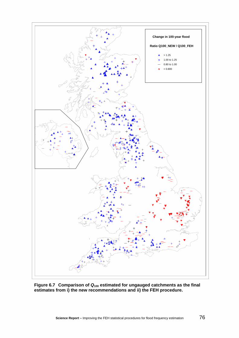
Science Report – Improving the FEH statistical procedures for flood frequency estimation 76
Change in 100-year flood
Ratio Q100_NEW / Q100_FEH
> 1.25
1.00 to 1.25
0.80 to 1.00
< 0.800
Figure 6.7 Comparison of Q100 estimated for ungauged catchments as the final estimates from i) the new recommendations and ii) the FEH procedure.

Science Report – Improving the FEH statistical procedures for flood frequency estimation 77
Change in QMED
Ratio QMED_NEW / QMED_FEH
> 1.25
1.00 to 1.25
0.80 to 1.00
< 0.800
Figure 6.8 Comparison of Q2 (QMED) estimated for ungauged catchments from i) the new recommendations and ii) the FEH procedure.

Science Report – Improving the FEH statistical procedures for flood frequency estimation 78
For comparison, Figure 6.8 is a copy of Figure 4.6, showing the changes in QMED (Q2) between the new recommendation and the FEH procedure. On comparing this map to Figure 6.7, which shows the ratios between the 100-year events, Q100, it is clear that it is the differences in the estimates of QMED that have the largest influence on the spatial pattern of the changes in Q100. This was to be expected, given the relative sizes of the changes in QMED and z100 that have been found. Table 6.10 summarises the results already quoted for the changes in QMED, the 100-year growth factor z100 and the 100-year flood, Q100.
Table 6.10 Summary of the effects of moving from the FEH procedures to the new recommendations
Percentage points of ratio (new / FEH) across 602 catchments
Quantity minimum 25% 50% 75% maximum QMED 0.55 1.00 1.15 1.24 2.01 z100 0.66 0.93 1.00 1.09 1.65 Q100 0.48 0.97 1.14 1.32 2.24

Science Report – Improving the FEH statistical procedures for flood frequency estimation 79
7 Default distribution The FEH (Vol. 3, Section 17.3.2) tested the goodness of fit of various candidate families of distributions, which suggested that the GLO distribution would be a generally applicable distribution for flood estimation in the UK. This test of fit was based on the work by Hosking and Wallis (1997: Section 5.2). A later report (Morris, 2003) raised the concern that the test of fit, as used in the FEH, was structured in such a way that the estimates of L-moment ratios used as the “pooling-group estimates” were calculated using a simple weighting scheme that was not the same as that put forward as the weighting scheme suggested to users of the FEH methodology, and concerns were raised that the results might be somewhat affected, or that at least there was some inconsistency.
7.1 The Hosking and Wallis test It should first be noted that, while Hosking and Wallis (1997) proposed their suggested test in a pooling-group context (“regionalisation” in their terminology), the test is applicable even to records for individual catchments. It is therefore of interest to consider in general terms the effect of the number of catchments in the pooling-group on this test, as this gives some guidance regarding the importance of the weighting scheme used within the test. The test is a comparison of the raw sample-based estimate of the L-Kurtosis with the value of the L-Kurtosis predicted by a fitted model. This difference is scaled by a value for the standard deviation which essentially measures how well the difference is estimated from the data contributing to the estimate of the difference. In the present circumstances, one may think of the difference in the L-Kurtosis values as being relatively fixed (if there really is a lack of fit) as more catchments are added to the pooling-group, while the variability of the difference decreases (because a better estimate of the difference is obtained by using data from extra catchments). Thus the standard deviation used for the devisor would go down and larger values of the test statistic would result, leading to more rejections of the hypothesis of an adequate fit, since the test-statistic is judged against a fixed critical value. The use of a larger pooling-group effectively increases the power of the test. However, the size of the pooling-group needs to be restricted to a size such that the assumption used within the test remains appropriate. Specifically, that it is reasonable to use a single common distribution to represent the standardised flood distribution for all catchments in the pooling-group.
The above considerations can be extended to consider the effects of spatial dependence on the test results. The values of the standard deviation used in the test are obtained by simulation of independently distributed flood-values for the catchments before these are combined, via weighted averages, into estimates of the 3rd and 4th L-moment ratios for the pooling-group. However, the presence of spatial dependence in the real data, and its absence in the simulated data, means that the simulations will under-estimate the variability of these pooled L-moment ratios. The standard deviation used as the divisor in the test will therefore be too small compared to the quantity that should ideally be used in the test. Thus (positive) spatial dependence will tend to lead to higher (more extreme) values of the test statistic, and this will lead to the null hypothesis that a given family of distribution fits being rejected too often compared to the target frequency for false rejections.
The role of the specific weighting scheme used to estimate the pooled L-moment ratios can also be considered. Firstly, it is important that exactly the same weighting scheme is used in calculating both the L-moment ratios used to calculate the difference of the L-Kurtosis values for the actual data, and for the equivalent steps when applied to the

Science Report – Improving the FEH statistical procedures for flood frequency estimation 80
simulated data. This has always been the case. Secondly, given this assumption, the effect of changing the weighting scheme for a given number of catchments will be similar to changing the number of catchments used in a fixed weighting scheme. Thus some weighting schemes may give more precise estimates of the difference of the two L-Kurtoses and lead to more power for the test. Using a weighting scheme within the test that is not “optimal” does not invalidate the test.
It should also be recalled that the test statistic suggested by Hosking and Wallis (1997) has been used not only for formal tests for whether there is enough evidence to reject the choice of a given 3-parameter family of distributions, but also as a way of indicating which of a number of families is “best”. In this instance, for a given pooling-group, equivalent test-statistics are calculated for a number of candidate families and the family for which the test-statistic is smallest (or indicates least lack-of-fit). This usage should not be badly affected by the problem relating to the inadequate representation of spatial dependence of the annual maximum values, since the statistics for each of the families should be affected roughly equally.
7.2 Revision of the Hosking and Wallis test On examining the principles behind the test of lack-of-fit as set-out by Hosking & Wallis (1997), a number of points arise. Some of these points are treated in more detail here. These considerations have led to the formulation of an alternative test-statistic which looks superficially similar to that of Hosking and Wallis, but the details of the calculations are rather different. A simulation-based study similar to that reported by Hosking and Wallis (1997; Table 5.2) has shown that the version of the statistic adopted here has properties which are superior to those of the original, in terms of having a much better match to the target acceptance rate of 90 per cent when the test is applied to cases where the distribution being tested is the same as the distribution from which the simulated data were generated
As discussed above, it seems likely that the effect of spatial dependence would mean that the variance estimated from independent samples would be too small and thus that more “rejections” of the individual tests would occur than the notional frequencies of 90 per cent acceptances and 10 per cent rejections for a critical value of Z of 1.64. The relative acceptability of the candidate distributions should be unaffected. In contrast, the effect of heterogeneity should be broadly neutral, provided that the distributions associated with each site are treated as fixed in the simulations.
Hosking and Wallis (1997) define the basis of their test-statistic in their Equation (5.3) in the following way, although a modified notation is used here. Firstly, the test is based on the idea that, for the 3-parameter distributions being treated, the theoretical value (according to the fitted distribution) of the L-Kurtosis can be evaluated and compared with the sample estimate of the L-Kurtosis obtained directly from the data. The existing methods of fitting the 3-parameter distributions that are being considered do not make any use of the sample L-Kurtosis and the basis of the test is to compare the sample L-Kurtosis with the model-derived L-Kurtosis for the fitted model. In practice, these model-derived values for the 4th L-moment ratio, DISTt4 , are obtained as a fixed (distribution-dependent) function of the L-Skewness (3rd L-moment ratio):
)( 34 tht DISTDIST =
where hDIST is the function that gives the theoretical L-Kurtosis in terms of the theoretical L-Skewness
)( 34 ττ DISTDIST h= ,

Science Report – Improving the FEH statistical procedures for flood frequency estimation 81
and where t3 is the sample L-Skewness. The basic form of the test statistic is defined as
4
44
σ
DISTDIST ttZ −
=
where 4σ represents a standard deviation to be discussed later. The sample L-Kurtosis, t4, and the sample L-Skewness, t3 (from which DISTt4 is derived) are both derived by a pooling-group scheme if more than one catchment is being considered, otherwise the usual single-catchment estimates would be used.
Note that Hosking and Wallis present a revised formulation (their equation (5.6)) which, with a reversal of sign to accord with the above, gives the final version of the test statistics as
4
444
σBttZ
DISTDIST −−
=
where B4 is a bias correction term. In the revised version used here, the bias correction term is much smaller than in the original and can be omitted without much effect. Hosking and Wallis (1997) gave a complicated expression for 4σ , involving B4, but this can be simplified to being identical to the sample variance of certain simulated quantities. In addition, Hosking and Wallis’s equation (5.6) is given with DIST
4τ instead of DISTt4 , presumably to indicate that the value is treated as fixed (see below).
According to the approach of Hosking and Wallis, 4σ should be the standard deviation of 4t . However, it is arguable that DIST
4σ should be the standard deviation of DISTtt 44 − , which might well be a rather smaller quantity. An alternative is that DIST
4σ should be the conditional variance of 4t given DISTt4 , but this would be rather more complicated to turn into a practical procedure. The question here is what should be treated as being the test statistic. The choices are 4t , ( )DISTtt 44 − or ( )DISTtt 44 . One of the revisions to the procedure that has been adopted here is to treat ( )DISTtt 44 − as the test statistic.
The Hosking and Wallis procedure is to test several families of distributions simultaneously for their lack of fit and to do so using a single base set of simulations from a Kappa distribution (which is a 4-parameter family of distributions). Thus the simulations are for a distribution which does not have theoretical L-moment ratios that correspond to ( )DISTttt 43 ,, , but rather has L-moment ratios ( )43 ,, ttt . While some arguments can be made that support this, it seems better to perform separate sets of simulations using whichever distribution is being tested to generate the simulated data. This eliminates several approximations and correction-terms that are required in the argument needed to support the use of a single common set of simulations.
7.3 The test procedure The procedure for testing the goodness of fit of a given family of distributions is as follows.
• Calculate the observed test statistic ( )DISTobs ttT 44 −= .
• Calculate a number, N, of simulated versions of the test statistic ( ){ }NiT isim ,,1; K=
using Monte Carlo simulations. Each of these simulated test statistics is calculated by constructing a set of data of the same size as the observed data (in terms of the number of sites in the pooling-group and the record lengths) independently between years and sites, from the distribution in the given family

Science Report – Improving the FEH statistical procedures for flood frequency estimation 82
which has the observed L-moment ratios ( )43 , tt and a unit mean. In particular, this means calculating simulated versions of 3t and 4t and then using the former to calculate )( 34 tht DIST
DIST = from the simulated value of 3t . Finally, the simulated values of the test statistic is calculated as ( ) ( )DISTi
sim ttT 44 −= .
• Calculate the sample mean 4B , and the sample variance, 24σ , from the set of
simulated test statistics ( ){ }NiT isim ,,1; K= .
• Calculate the test statistic 4
444
σBttZ
DISTDIST −−
= .
• Compare the absolute value DISTZ with 1.64, and count the fit as acceptable if 64.1≤DISTZ . Otherwise reject the particular family of distributions for the
particular pooling-group.
As noted earlier, the bias correction 4B is small and can be omitted. It is important that the test statistics carried over from the individual simulated data sets are the differences ( ) ( )DISTi
sim ttT 44 −= and not just the L-kurtosis 4t as used by Hosking & Wallis (1997).
7.4 Results This section summarises the results obtained by applying the test procedure outlined above in Section 7.2 to pooling-groups formed as outlined in Chapter 6 (considering the catchment to be ungauged) for each of the 602 catchments used in this study. The following five 3-parameter distributions were considered as possible candidate distributions:
• Generalised Logistic (GLO).
• Generalised Extreme Value (GEV).
• Generalised Normal (GNO), also known as the 3-parameter Log-Normal.
• Person type 3 (PE3).
• Generalised Pareto (GPA).
For a further description of each of these distributions, please refer to the FEH (Vol. 3, Chapter 15) or Hosking and Wallis (1997).
The results of the analysis are summarised in Table 7.1, where the first row (labelled “Chosen”) contains the number of times (out of 602) that a particular distribution was chosen as the preferred option (smallest value of DISTZ ). The second row (labelled “Accepted”) contains the number of times a particular distribution gave a value of the test statistic satisfying 64.1≤DISTZ . Finally, the last row (labelled “Rejected”) counts the number of times a particular distribution was rejected.
Table 7.1 Results of the goodness of fit test applied to pooling-groups formed for each of the 602 catchments.
Test GLO GEV GNO PE3 GPA Chosen 283 167 106 46 0 Accepted 364 358 339 209 0 Rejected 238 244 263 393 602

Science Report – Improving the FEH statistical procedures for flood frequency estimation 83
From the results in Table 7.1, it is clear that the GLO distribution remains the best choice for a default UK distribution as it is both chosen and accepted more often than any of the other candidate distributions. However, the results for the two distributions are somewhat closer than reported for the FEH study. The numbers of catchments for which the GLO and GEV distributions are “accepted” are almost equal, but the comparison favours the GLO marginally. While it appears that the main distinction in the results between the GLO and GEV distributions lies in the number of times that the distribution is chosen as having the “best” fit, it should be recalled that this comparison is affected by which other distributions have been included in the competing set. It is not clear how many of the catchments which have the GNO, PE3 and GPA distributions as their “chosen” distributions would select the GLO if the only options were GLO and GEV.

Science Report – Improving the FEH statistical procedures for flood frequency estimation 84
8 Summary of new flood estimation procedures This chapter provides a short summary of the new procedures introduced in this project. While maintaining the conceptual basis of the index-flood method, as implemented in the FEH, the work undertaken in the current project has improved the estimation of QMED and the growth curve at both gauged and ungauged catchments.
8.1 Estimation of QMED The recommended method for estimating the index flood (QMED) depends on whether the subject site is a gauged or an ungauged catchment.
8.1.1 Estimating QMED at a gauged catchment
Detailed guidelines for estimation of QMED from flood data were provided as part of the FEH (Vol.3 Ch. 2). No further investigation into this aspect of the method has been undertaken as part of this study. Note that for the development of the regression model linking QMED to catchment descriptors (the QMED model) in the current study, all sample values of QMED were estimated as the median of the AMAX series regardless of record length. Also, the QMED values were not subjected to adjustment for climatic variation as in the FEH.
8.1.2 Estimating QMED at an ungauged catchment
When no flood data are available at the site of interest, QMED has to be estimated either from catchment descriptors (possibly including data transfer from a nearby gauged donor catchment) or using some other method.
Catchment descriptors
The QMED for rural catchments can be estimated as
2
0460.01536.03062.8 4451.31000
8510.0 BFIHOSTSAAR FARLAREAQMED⎟⎠⎞
⎜⎝⎛
= . (8.1)
The catchment descriptors are available from the FEH CD-ROM Version 2 for all catchments in the UK larger than 0.5 km2. The factorial standard error (fse) of the estimated QMED values is 1.431, which is a 7.5 per cent reduction compared to the fse value of 1.541 reported for the original FEH QMED equation.
The FEH emphasises that the uncertainty of QMED estimated using the QMED equation is generally much larger than the uncertainty of estimates obtained directly from flood data. Consequently, the FEH recommends that data transfer from nearby gauged donor or analogue catchments should be used wherever possible. However, based on research by Kjeldsen and Jones (2007) and results obtained in this study, it is found that the benefits of donor sites are generally less than previously thought. It is therefore recommended that the data transfer procedure is revised to account for the

Science Report – Improving the FEH statistical procedures for flood frequency estimation 85
geographical distance between the centroids of the target catchment and a donor catchment as
sga
cdsg
obsgcdssadjs QMED
QMEDQMEDQMED ⎟
⎟⎠
⎞⎜⎜⎝
⎛=
,
,,, , (8.2)
where
⎟⎠⎞
⎜⎝⎛⎟
⎠⎞⎜
⎝⎛⎟
⎠⎞
⎜⎝⎛ −−+−= sgsgsg dda 4785.0exp4598.010200.0exp4598.0 ,
and where sgd is the geographical distance (km) between the subject site and the gauged donor site.
The donor adjustment in the form given in equation (8.2) will automatically reduce the influence of the donor site as the geographical distance between the two catchment centroids increases. For example, the adjustment term asg is less than 0.1 when the inter-centroid distance is greater than about 76km.
Other methods
The FEH provided tentative advice on other methods for estimating QMED when no flood data are available, including obtaining QMED from rainfall-runoff modelling and a relationship between QMED and river channel dimensions. No research has been undertaken as part of this study to further investigate and improve the usefulness of these methods.
8.2 Estimation of the growth curve The estimation of the growth curve is based on the pooling-group method and requires i) the formation of a pooling-group followed by ii) estimation of the pooled distribution parameters through the method of L-moments using the weighted average of the L-moment ratios within the pooling-group.
8.2.1 Selecting a pooling-group
As in the FEH, a pooling-group for a particular site of interest is formed by identifying a number of gauged catchments classified as hydrologically similar. The selection of catchments is based on a distance measure, measuring the distance in a catchment descriptor space defined by ln[AREA], ln[SAAR], FARL and FPEXT and calculated as
.04.0
2.0
05.01.0
37.0lnln
5.028.1
lnln2.3
2
222
⎟⎟⎠
⎞⎜⎜⎝
⎛ −+
⎟⎟⎠
⎞⎜⎜⎝
⎛ −+⎟⎟
⎠
⎞⎜⎜⎝
⎛ −+⎟⎟
⎠
⎞⎜⎜⎝
⎛ −=
ji
jijijiij
FPEXTFPEXT
FARLFARLSAARSAARAREAAREASDM
(8.3)
The FEH recommended that the size of the pooling-group should vary according to the target return period such that the total number of AMAX events should be at least 5

Science Report – Improving the FEH statistical procedures for flood frequency estimation 86
times the return period (the 5T rule). However, it was found that a default pooling-group size consisting of 500 AMAX events performed well for a range of return periods.
Detailed instructions of how to review and adapt the initial pooling-group were presented in the FEH. The main differences between the FEH and the revised method presented here are due to the new weighting scheme presented in the next section, however the main points of difference are summarised below. Firstly, the new weighting scheme assigns weight to each individual catchment in the pooling-group based on the distance in catchment space from the target site rather than on rank within the pooling-group. Hence, moving catchments up or down in the ranking order within the pooling-group will not change the weights. Secondly, the weighting scheme will differentiate between a gauged and an ungauged catchment and derive weights differently for the two cases. Finally, two separate sets of weights are used for the calculation of pooled L-CV and L-SKEW values.
8.2.2 Estimating the pooled growth curve
As in the FEH, the pooled growth curve is derived using the pooled L-moment ratios derived from the M sites in a pooling-group. For a GLO distribution, the mathematical form of the pooled growth curve is defined as
( )( )P
Tz P
PPT
κ
κβ 111 −−+= , (8.4)
where the superscript P indicates that a parameter is based on pooled data. The pooled GLO parameters are estimated using the pooled L-moment ratios as
( )( ) ( ).ˆsinˆˆ
ˆsinˆˆ
,ˆ
22
2
3
PPPP
PPPP
PP
ttt
t
κπκπκκπκβ
κ
−+=
−= (8.5)
The pooled L-moment ratios, Pt2 and Pt3 , are calculated as the weighted average of the L-moment ratios for each individual catchment in the pooling-group. For both L-CV and L-SKEW, the weighted average is defined as
∑=
=M
jjrj
Pr tt
1,ω (r = 2,3), (8.6)
where the weights depends on whether or not the site of interest is gauged or ungauged, the record length and the distance in catchment descriptor space from the target site for each individual site. Whereas the FEH used the same set of weights for both L-CV and L-SKEW, this study has developed a different set of weights for each of the two L-moment ratios.
No information at target catchment (ungauged)
For a pooling-group created for an ungauged site, the weights assigned to L-CV and L-SKEW for each catchment are defined as
L-CV ( )( )∑
=
−
−
+
+= M
kkk
jjj
bc
bc
1
1̀
1
ω , j = 1,…,M. (8.7)

Science Report – Improving the FEH statistical procedures for flood frequency estimation 87
L-SKEW ( )( )∑
=
−
−
+
+= M
kkk
jjj
bc
bc
1
1
1
ω , j = 1, …,M. (8.8)
In the above, the quantity bj is defined separately for L-CV and L-SKEW as
L-CV ⎟⎠⎞
⎜⎝⎛ +=
20023.00047.0 jj SDMb , (8.9)
L-SKEW ⎟⎟⎠
⎞⎜⎜⎝
⎛⎥⎦
⎤⎢⎣
⎡−−=
2360.0exp10219.0 j
j
SDMb , (8.10)
and the sampling variance ck is defined for L-CV and L-SKEW as
L-CV 1
02609.0−
=k
k nc (8.11)
L-SKEW 2
2743.0−
=k
k nc (8.12)
where nk is the record-length at the k’th site. Details of the development of equations (8.9) to (8.12) are provided in Chapter 6.
Data available at the subject catchment (gauged)
When data are available at the subject catchment, a special (large) weight is assigned to the at-site data (catchment number j = 1) to emphasise the importance of at-site data compared to the other catchments in the pooling-group. When conducting a pooled analysis at a gauged site, different sets of weights are used for L-CV and L-SKEW.
For L-CV, the weighting scheme for a gauged catchment is defined as
( )( )∑
=
−
−
+
++
+= M
kkk bc
bccbc
b
1
1
211
111
11ω , j = 1 (8.13)
( ) ( )( )∑
=
−
−−
+
++= M
kkk
jjj
bc
bcbcc
1
1
11111ω , j = 2,…,M (8.14)
The quantity bj is defined in equation (8.9) and the sampling variance cj is defined in equation (8.11).
For L-SKEW, the weighting scheme used for gauged catchment is similar to the scheme used for the ungauged catchment:
( )( )∑
=
−
−
+
+= M
kkk
jjj
bc
bc
1
1
1
ω , j = 1, …,M. (8.15)

Science Report – Improving the FEH statistical procedures for flood frequency estimation 88
Again, details of bj and cj can be found in equations (8.10) and (8.12), respectively. Note that for the gauged case, the first catchment (j = 1) in the pooling-group is the actual target site and therefore SDMsj is the distance from the target site to itself and therefore b1 equals zero for L-SKEW. In the ungauged case, the distance between the (ungauged) target site and the first member of the pooling-group is larger than zero (with the exception of the very unlikely case where the two catchments have identical catchment descriptor values of ln[AREA], ln[SAAR], FARL and FPEXT).
8.3 Estimation of the flood frequency curve The index-flood method constructs the flood frequency curve, xT , as a product of the index flood, QMED, and the dimensionless growth curve, zT, as
TT zQMEDx = , (8.16)
where T is the return period in years. When the growth curve is obtained using the pooling-group procedure (Section 8.2), zT is obtained as P
Tz in equation (8.4).

Science Report – Improving the FEH statistical procedures for flood frequency estimation 89
9 Conclusions The research presented in this report constitutes an improvement to the existing FEH statistical procedures for flood frequency estimation. The improvements are a result of both i) new modelling techniques and ii) an updated data set (HiFlows-UK). The statistical procedures outlined in the FEH made the region-of-influence approach operational in the UK, which was considered a major achievement and a benchmark for research and development both nationally and internationally. As a result, the new developments introduced in this project build on the foundations laid by the FEH and further improve the reliability of flood frequency estimation in the UK.
9.1 Improved modelling techniques The model developments carried out in this project focused on three main aspects: i) improving the QMED equation, ii) revising the procedure for using data transfer from gauged donor sites to ungauged sites, and iii) the pooling procedure for estimation of growth curves at both gauged and ungauged sites. All three aspects of the method have been improved while retaining the general work-flow of the original FEH methodology.
Many of the improvements introduced through the development of the new QMED equation and the associated data transfer procedure are based on research carried out at CEH, particularly that of Kjeldsen and Jones (2006, 2007), identifying the linkage between the underlying structure and estimation of the QMED regression model and an optimal procedure for transfer of data from a gauged donor catchment to an ungauged subject catchment. In particular, this project has shown that identification of potential donor catchments should be based on geographical closeness rather than being based on ‘hydrological similarity’ as defined by catchment descriptors. Consequently, it is recommended that analogue catchments should no longer be used for adjusting QMED estimates obtained using the QMED equation. This is the case for both the existing FEH methodology and the new procedure introduced in this project. This is considered an important finding that should have significant influence on the current practical FEH procedures.
Through careful examination of the regression residuals from a number of potential QMED models, it was possible to identify a new QMED model that performs better than the FEH model while using only four catchment descriptors (compared to the six used in the FEH equation). The set of four catchment descriptors in the new equation is considered a more intuitive combination than that of the FEH equation and the project has managed to remove the RESHOST variable, which is not generally well-understood.
The revised procedure for estimation of the growth curve at ungauged sites using pooling-groups showed some improvements over the existing FEH procedure. However, the improvements were less significant than those observed in the QMED modelling part of the project. This is a result of the fundamental difficulty in flood frequency analysis that the higher order statistical moments of the flood series (L-CV and L-SKEW) that determine the growth curve have large sampling variances. They thus require longer series of observations than, for example, QMED to obtain reliable estimates of the true values. The high degree of sampling variability allows only weak relationships to be formed between the growth curves and catchment descriptors, hence the poor performance. The problem is illustrated by the fact that regression models linking L-CV and L-SKEW to catchment descriptors in FEH were found to have

Science Report – Improving the FEH statistical procedures for flood frequency estimation 90
r2 values of 37.5 per cent and 8 per cent respectively, while the equivalent result for QMED was in the excess of 90 per cent.
Based on results from an extensive exploratory analysis the FEH definition of 'hydrological similarity' used for creating pooling groups was revised. The FEH definition of hydrological similarity was based on similarity of a subject site with regards to ln[AREA], ln[SAAR] and BFIHOST. The revised procedure presented in this report replaced BFIHOST with ln[FARL] and ln[FPEXT], while retaining ln[AREA] and ln[SAAR], as this combination of catchment descriptors was found to provide more accurate prediction of pooled growth curves at ungauged catchments (see Table 6.3). Also, see Section 9.2.6 for a further discussion of the problem of pooled frequency analysis on permeable catchments.
An important aspect of the improved methodology is the introduction of two separate weighting schemes for L-moment ratios within a pooling-group based on whether the pooling-group is formed for a gauged or an ungauged catchment. By first defining the statistical model underlying the pooling procedure (Appendix D), it was found that available at-site data should be given relatively more weight compared to the other sites in a pooling-group.
9.2 HiFlows-UK Underlying the research presented in this report is the annual maximum peak flow data made available from the HiFlows-UK data project. The FEH recommends that POT data should be used for deriving estimates of QMED for short record lengths, where “short” is defined as less than 14 years of data. The initial review of the HiFlows-UK data found a number of practical issues with the updated POT dataset which could not reasonably be amended within this project. Consequently, POT data were not used in this study.
Compared to the dataset used in the development of the original FEH methodology, the extra quality control checks introduced in the HiFlows-UK project led to a reduction in the total number of gauged catchments used in the development of the method; specifically a reduction from 728 in the FEH to 602 in this study. However, the general increase in record length from an average of 22.7 years in the FEH to 32.7 years in this study ensured that the total number of AMAX events used in this study is 19 per cent greater than the number used in the FEH (see Table 2.1).
The extra quality control combined with the extended record length was reflected in the model development part of this study. In particular, the model diagnostics plots used for assessing the new QMED model clearly showed a better alignment between the regression model and the underlying data than that obtained in the development of the original FEH model. While the comparisons between the new and the FEH pooling procedures were undertaken based on HiFlows-UK data, the extended record lengths in HiFlows-UK will undoubtedly have a large effect on the estimated higher order L-moment ratios (L-CV and L-SKEW) by reducing their sampling variability. This allowed for a more robust pooling procedure to be developed, since a better relationship between the growth curves and the catchment descriptors could be identified, as reflected in the comparison between the methods (see Table 6.3).
9.3 Future direction of research and development The objective of this project was to improve the existing statistical procedure outlined in the FEH Vol. 3. The current project has successfully achieved the following tasks.

Science Report – Improving the FEH statistical procedures for flood frequency estimation 91
• Improved the estimation of QMED from catchment descriptors.
• Provided a more robust method for data transfer from gauged to ungauged catchments.
• Provided an improved method to derive flood growth curves for both gauged and ungauged catchments using pooling groups.
However, the scope of this project did not encompass all aspects of the FEH methodology. Also, during the course of the project, particular parts of the methodology were identified where further research and development would be beneficial. This section provides a discussion of subjects where further research and development would provide further improvements of flood frequency estimation in the UK.
9.3.1 HiFlows-UK database
Given the importance of flood estimation to the UK in general terms, and given also the major role that the HiFlows-UK database plays in providing data for this task, there is a clear imperative to maintain and improve this resource. The FEH-based procedures have been constructed to enable good use to be made of any updates to the HiFlows-UK database, as soon as they are available.
Besides simply extending the records at the existing set of catchments included in HiFlows-UK, it is important to consider whether these catchments are sufficiently representative of catchments where flood estimation problems arise in practice. In particular, a view has been expressed by users of FEH methodology that they are often concerned with catchments that are rather smaller than those included in the HiFlows-UK data-set. Future research should pay particular attention to collection of hydrometric data and the performance of FEH methodologies on small catchments.
9.3.2 Flood peak data
While the HiFlows-UK database of AMAX events is a welcome development and while it has provided an improved dataset, it was regrettable that the general quality of the POT series was not found to be of a similar good quality. Flood frequency analysis based on AMAX series is a long established practice both in the UK and elsewhere. However, there are strong theoretical results that show that more reliable estimates of floods can be obtained when using statistical models developed for use with POT data. Furthermore, as the statistical models underlying the POT method are based on more mechanistic principles than the empirical distribution fitting used in AMAX modelling, POT models are more suitable for testing sensitivity of flood frequency to changes in flood-generating mechanisms. It is therefore recommended that research should be initiated to develop a national procedure for flood frequency estimation based on POT models. This would rely on there being a substantial improvement in the HiFlows-UK database regarding the details of the valid/invalid periods of the POT data records.
9.3.3 Flood frequency and environmental change
A very important aspect of flood frequency analysis in flood risk management is the potential effect of environmental change, such as urbanisation and climate change, on flood frequency characteristics. Traditionally, methods based on the statistical analysis of historical records have not been particularly well-suited for predicting the results of changes in the mechanisms which generate floods, and hence emphasis has been put on more conceptual hydrological models, such as the rainfall-runoff based approaches.

Science Report – Improving the FEH statistical procedures for flood frequency estimation 92
However, considering the relatively large amount of data underpinning the statistical method, it seems reasonable to develop empirical and robust measures for predicting the effect of environmental change as observed within the dataset. It is recommended that two particular aspects of environmental change of interest to flood managers should be further investigated.
Urbanisation
While the qualitative effect of increased urbanisation on flood response from a catchment is well understood (increase in the percentage runoff and decrease in the response time) the challenge in applied hydrology is to quantify these effects and to make a generally applicable model. Initial work on quantifying the effect of urbanisation using flood frequency models was reported by Packman (1980), which formed the basis for the procedure developed for the FEH statistical procedure. Later, Bayliss et al. (2006) updated the procedure to use URBEXT2000 rather than URBEXT1990 (as in the FEH) with some minor changes to the methodology as recommended by Morris (2003). To further improve the ability to predict the effect of urbanisation on the flood frequency characteristics for a particular catchment, it is necessary to undertake a critical review of the current adjustment procedures. In particular, the empirical adjustment factors should be formulated in a statistical framework to enable inference regarding the significance of any detected effects compared to the general variability observed in the flood peak data. Also, data characterising the temporal development of urbanisation should be collected and analysed for selected catchments, thereby providing detailed information on the effect of urbanisation on peak flow data. An excellent opportunity for research is provided by the HiFlows-UK database combined with measures of urbanisation derived from land cover maps such as URBEXT1990, URBEXT2000, and a potential new URBEXT measure based on new maps of land cover representing 2007.
Climate change
The current statistical method is based on assumptions of a stationary climate. The estimates from the method can, in some circumstances, be adjusted in order to make projections of the impacts of climate change. While it is generally accepted that climate change will have an impact on large-scale rainfall and runoff patterns, there is less certainty about the climate change signals detected from the analysis of observed time series of rainfall and runoff. In particular, little is known about the impact of climate change on extreme events. A comprehensive study investigating the existence of trends and shifts in the FEH dataset by Robson and Reed (1999) concluded that “Climate change cannot be clearly detected in the FEH datasets”. However, since the publication of the FEH, the need for predicting and mitigating the potential effects of climate change has become of greater concern. Thus, despite weak signals of climate change being observed in historical flood data, research is urgently needed to i) identify the likely impact of climate change on the characteristics of future hydrological extremes and, ii) to develop a framework for estimating and reporting useful measures of the future probability of occurrence of extreme events. The specific activities that need to be undertaken are:
i) To refine and apply appropriate statistical tests for an exploratory investigation of change (trends, shifts and long-term periodic cycles) in long-term time series of observed river flow. An investigation should focus on the identification of temporal variability in both mean values and variability of observed time series. In particular, the study should seek to quantify changes in different seasons.

Science Report – Improving the FEH statistical procedures for flood frequency estimation 93
ii) Develop statistical extreme value models that can be applied in non-stationary environments, such as a changing climate. These models will allow for specification of identified and projected changes in the statistical properties of the extreme processes.
9.3.4 Catchment descriptors
The existing set of descriptors is probably as good as possible given the existing underlying datasets. They are wide-ranging in terms of types of properties being measured. One set of descriptors that might possibly be useful are quantities to measure diversity within a catchment. Of course, some of the existing measures do relate to diversity within the catchment, but other aspects such as soil and geology might be brought into consideration.
Possible improvements to the underlying data sources include the following.
• An improved HOST dataset, providing better quality data at a finer spatial resolution – but this would entail a recalibration of the HOST-derived quantities (BFIHOST, SPRHOST)
• An updated set of URBEXT descriptors might be based on the forthcoming land-cover map 2007.
There is also the possibility of making some minor improvements in the formulation of some of the existing catchment descriptors in an attempt to overcome some of the problems reported by Morris (2003) relating to how these vary when moving along a river channel.
9.3.5 Use of donor catchments
A very important improvement to the FEH procedure presented in this report is the revised procedure for estimation of QMED using data transfer from a gauged donor catchment to an ungauged subject catchment. While the new donor procedure is an important improvement, it is currently limited by allowing only one potential donor site to be used. Further model development and testing is necessary to allow more than one donor catchment to be used and to assess the effect of such a methodological extension.
Within the new framework for using donor catchments, this project initiated work on distinguishing between a donor catchment located on the same river network as the subject catchment and other donor catchments. More work is needed to further classify donor catchments according to location relative to donor catchments before such a system could be made operational. However, it would be an intuitive extension to the framework and could potentially add further improvements to the method.
9.3.6 Use of pooling-groups
The pooling-group method is a flexible tool allowing new and updated data to be used as they become available through HiFlows-UK. Consequently, the pooling-group method was retained in this project.
The improved method presented in this report distinguishes between a pooling-group formed for a gauged or an ungauged catchment and defines the weights given to the L-moment ratios for each catchment accordingly. Further model development could be undertaken to account for the intermediate case where a pooling-group is created for an ungauged catchment but data from a nearby gauged catchment are available.

Science Report – Improving the FEH statistical procedures for flood frequency estimation 94
These could be used in a manner similar to the donor transfer scheme defined for estimation of QMED at ungauged catchments. Further research would be needed to identify and quantify the underlying structure of the model errors arising from use of the pooling-group method.
As in the FEH, the formation of pooling-groups in the improved method is based on the the concept of hydrological similarity as defined by a set of catchment descriptors. However, the actual definition of hydrological similarity has been changed in this study, with the substitution of BFIHOST with FARL and FPEXT (retaining ln[AREA] and ln[SAAR]). This was a reasonable choice based on a thorough investigation of predictive ability of the catchment descriptors, but it does leave the method without any special attention being paid to growth curve estimation on permeable catchments -- the effect in FEH might have been largely illusory. It has been suggested that flood peak data from permeable catchment can exhibit what could be realisations from two distinct flood-generating mechanisms. It is recommended that further research should be undertaken to investigate the existence of such multiple mechanisms and, if confirmed, to determine how to incorporate such effects into the current procedures.
The use of pooling-groups (or regional methods in general) for enhancing single-site estimation is often referred to as “substituting space for time”. Among applied hydrologists there is a very reasonable attraction in trying to extend the flood data series extracted from systematic flow records back in time with more anecdotal evidence of large flood events that occurred before the systematic recordings were initiated and often pre-dating living memory. To support such activities, efforts have been made to compile and make available, through an on-line archive (http://www.dundee.ac.uk/geography/cbhe/), information on historical flood events on UK rivers (Black and Law, 2004). Unfortunately, these endeavours have not been matched by associated methodological developments for incorporating such information into flood frequency analyses based on data from systematic records. A further development of the existing FEH methodology would to combine both types of information in an overall flood frequency analysis. This would provide a significant development and effectively bring together long-standing efforts made by the gauging authorities, the British Hydrological Society, the academic community and a myriad of individuals to provide an improved methodology.

Science Report – Improving the FEH statistical procedures for flood frequency estimation 95
References ACREMAN, M. AND WILTSHIRE, S. E., 1987. Identification of regions for regional frequency analysis (abstract), Eos Transaction. AGU, 68(44), 1262
ACREMAN, M. AND WILTSHIRE, S. E., 1989. The regions are dead; long live the regions. Methods of identifying and dispersing with regions for flood frequency analysis. In: FRIENDs in Hydrology, edited by L. Roalds et al., IAHS Publ. 187, 175-188.
BAYLISS, A. C. 1999. Catchment descriptors. Volume 5, Flood Estimation Handbook, Institute of Hydrology, Wallingford.
BAYLISS, A. C., BLACK, K. B., FAVA-VERDE, A. AND KJELDSEN, T. R., 2006. URBEXT2000 – A new FEH catchment descriptor: Calculation, dissemination and application. R&D Technical Report FD1919/TR, Department for Environment, Food and Rural Affairs, London, UK.
BLACK, A. R AND LAW, F. M., 2004. Development and utilization of a national webbased chronology of hydrological events. Hydrological Sciences Journal, 49(2), 237-246.
BURN, D. H., 1990. Evaluation of regional flood frequency analysis with a region of influence approach. Water Resources Research, 26(10), 2257-2265.
CENTRE FOR ECOLOGY & HYDROLOGY (2007) FEH CD-ROM Version 2.0. Centre for Ecology & Hydrology, Wallingford, UK.
COLE, G., 1965. An application of the regional analysis of flood flows. Institution of Civil Engineers, Symposium on River Flood Hydrology (published 1966), London, 39-57.
DALRYMPLE, T., 1960. Flood frequency analysis. Water Supply Paper 1543-A, U.S. Geological Survey, Reston, Va., USA.
DAWSON, C. W., ABRAHART, R. J., SHAMSELDIN, A. Y. AND WILBY, R. L., 2006. Flood estimation at ungauged sites using artificial neural networks. Journal of Hydrology, 319, 391-409
FAULKNER, D. S., 1999. Rainfall frequency estimation. Volume 2 Flood Estimation Handbook, Institute of Hydrology, Wallingford, UK.
GORE, W. AND THOMSON, H., 1909. Note on rainfall and stream flow statistics. Geographical Journal, vol. 34, p645.
GUMBEL, E. J., 1941 Probability interpretation of observed return period of floods, Transactions of the American Geophysical Union, Part III, 836-850.
HORTON, R. E., 1913. Flood frequency and flood control. Engrg. Record, vol. 68.
HOSKING, J. R. M. AND WALLIS, J. R., 1997. Regional Flood Frequency Analysis: an approach based on L-moments. Cambridge University Press, New York.
HOSKING, J. R. M., WALLIS, J. R. AND WOOD, E. F., 1985. An appraisal of the regional flood frequency procedure in the UK Flood Studies Report, Hydrological Sciences Journal, 30(1), 85-109.
INSTITUTE OF HYDROLOGY, 1983. Some suggestions for the use of local data in flood estimation. Flood Studies Supplementary Report No. 13, Institute of Hydrology, Wallingford, UK.

Science Report – Improving the FEH statistical procedures for flood frequency estimation 96
INSTITUTE OF HYDROLOGY, 1999. Flood Estimation Handbook, 5 Volumes, Wallingford, UK.
JENKINSON, A. F., 1955. The frequency distribution of the annual maximum (or minimum) values of meteorological elements. Quart. Jour. Roy. Met. Soc., 81, 158-171.
KJELDSEN, T. R. AND JONES, D. A., 2004. Sampling variance of flood quantiles from the generalised logistic distribution estimated using the method of L-moments. Hydrological and Earth System Sciences, 8(2), 183-190.
KJELDSEN, T. R. AND JONES, D. A., 2006. Prediction uncertainty in a median-based index flood method using L moments, Water Resources Research, 42, W07414, doi:10.1029/2005WR004069
KJELDSEN, T. R. AND JONES, D. A., 2007. Estimation of an index flood using data transfer in the UK. Hydrological Sciences Journal, 52 (1), 86-98.
KJELDSEN, T. R. AND JONES, D. A., 2008. An exploratory analysis of error components in hydrological regression modelling. To appear in Water Resources Res.
KJELDSEN, T. R., STEWART, E. J., PACKMAN, J. C., FOLWELL, S. S., AND BAYLISS, A. C. (2005) Revitalisation of the FSR/FEH rainfall-runoff method. R&D Technical Report FD1913/TR, Department for Environment, Food and Rural Affairs, London, UK.
MERZ, R. AND BLÖSCHL, G., 2005. Flood frequency regionalisation—spatial proximity vs. catchment attributes. Journal of Hydrology, 302 (1-4), 283-306.
MORRIS, D.G. (2003) Automation and appraisal of the FEH statistical procedures for flood frequency estimation. Final report to Defra. Centre for Ecology & Hydrology, Wallingford, 207pp.
MORRIS, D.G. AND FLAVIN, R.W., 1996. Flood risk map for England and Wales. IH Report No. 130, Institute of Hydrology, Wallingford, UK.
NASH, J.E. and SHAW, B.L., 1965. Flood frequency as a function of catchment characteristics. Institution of Civil Engineers, Symposium on River Flood Hydrology (published 1966), London, 115-136.
NERC (1975) Flood Studies Report. 5 Volumes, Natural Environment Research Council, London.
PACKMAN, J. C., 1980. The effect of urbanisation on flood magnitude and frequency. IH Report No. 63, Institute of Hydrology, Wallingford, UK.
RIJAL, N. AND RAHMAN, A., 2005. Design flood estimation in ungauged catchments: quantile regression technique and probabilistic rational method compared. In: MODSIM2005 International Congress on Modelling and Simulation, A. Zerger and R.M. Argent (eds), Modelling and Simulation Society of Australia and New Zealand, December 2005, 1887-1893.
ROBSON, A. AND REED, D., 1999. Statistical procedures for flood frequency estimation. Volume 3 Flood Estimation Handbook, Institute of Hydrology, Wallingford, UK.
STEDINGER, J.R., VOGEL, R.M. AND FOUFOULA-GEORGIOU, E. 1993. Frequency analysis of extreme events. Chapter 18 in Handbook of Hydrology (ed. D. R. Maidment), McGraw-Hill, USA.
SUTCLIFFE, J. V., 1978. Methods of flood estimation: A guide to the Flood Studies Report. IH Report No. 49, Institute of Hydrology, Wallingford, UK.

Science Report – Improving the FEH statistical procedures for flood frequency estimation 97
TASKER, G. D. AND STEDINGER, J. R., 1989. An operational GLS model for hydrological regression. Journal of Hydrology, 111, 361-375.
WALLIS, J.R., 1981. Risk and unceratintiesin the evaluation of flood events for the design of hydraulic structures. In: Pienne e Siccità (ed E.Guggino, G. Rossi, E. Todini), 3-36, Fondazione Politecnica del Mediterraneo, Catania, Italy.
WOLF, P. O., 1965 Comparison of methods for flood estimation. In: Institution of Civil Engineers Symposium on River Flood Hydrology (1966), 1-23.

98
Appendix A QMED values and gauge details No. River Gauging station Easting Northing No. of
years Start End Date of
maxFlow max
QMED No.
2001 Helmsdale Kilphedir 284324 929794 28 1975 2002 06-Oct-1993 272.37 169.06 2001 2002 Brora Bruachrobie 274462 916259 10 1993 2002 06-Dec-1999 205.49 143.55 2002 3002 Carron Sgodachail 240482 888010 29 1974 2002 21-Feb-2002 342.78 184.24 3002 3003 Oykel Easter Turnaig 231271 901365 25 1978 2002 05-Oct-1978 823.53 342.06 3003 4003 Alness Alness 253141 877497 29 1974 2002 07-Oct-1993 252.97 82.21 4003 4005 Meig Glenmeannie 220273 850353 18 1985 2002 16-Jan-1993 212.75 114.89 4005 4006 Bran Dosmucheran 212722 856678 14 1989 2002 02-Jan-1992 120.8 85.16 4006 6003 Moriston Invermoriston 221387 812362 14 1930 1943 20-Dec-1936 554.88 312.92 6003 6008 Enrick Mill of Tore 238353 828104 24 1979 2002 01-Mar-1997 97.17 51.33 6008 7001 Findhorn Shenachie 273215 821452 26 1977 2002 20-Sep-1981 485.52 268.21 7001 7002 Findhorn Forres 284034 830206 45 1958 2002 16-Aug-1970 1112.63 312.01 7002 7003 Lossie Sheriffmills 314502 853471 45 1958 2002 16-Nov-2002 151.35 43.43 7003 7004 Nairn Firhall 273722 837368 22 1981 2002 01-Jul-1997 314.11 105.51 7004 7005 Divie Dunphail 301689 839889 21 1982 2002 01-Jul-1997 141.65 60.44 7005 8001 Spey Aberlour 292139 810489 62 1938 2002 17-Aug-1970 1179.31 415.62 8001 8002 Spey Kinrara 270711 793742 52 1951 2002 18-Dec-1966 361.53 140.47 8002 8004 Avon Delnashaugh 316609 817588 51 1952 2002 02-Oct-1981 521.3 221.37 8004 8005 Spey Boat of Garten 275066 796799 52 1951 2002 18-Dec-1966 392.79 163.75 8005 8006 Spey Boat o Brig 294879 812741 51 1952 2002 17-Aug-1970 1059 472.09 8006 8007 Spey Invertruim 258191 791354 51 1952 2002 17-Dec-1966 274.68 100.81 8007 8008 Tromie Tromie Bridge 276489 786784 51 1952 2002 06-Sep-1958 116.54 50.92 8008 8009 Dulnain Balnaan Bridge 285086 819396 51 1952 2002 05-Feb-1990 172.26 94.4 8009 8010 Spey Grantown 279940 802927 51 1952 2002 06-Feb-1990 507.15 223.91 8010 8011 Livet Minmore 324546 823506 23 1980 2002 02-Oct-1981 51.82 31.04 8011 9001 Deveron Avochie 344243 831607 44 1959 2002 15-Nov-2002 258.22 123.32 9001 9002 Deveron Muiresk 348674 840599 44 1959 2002 12-Sep-1995 494.04 247.67 9002 9003 Isla Grange 341980 850067 44 1959 2002 01-Jul-1997 96.07 46.41 9003 9004 Bogie Redcraig 348530 829933 23 1980 2002 15-Nov-2002 95.61 27.43 9004
10001 Ythan Ardlethen 381351 839185 46 1939 1984 06-Nov-1951 104.03 50.18 10001 10002 Ugie Inverugie 396184 850658 32 1971 2002 23-Oct-2002 147.79 46.83 10002 10003 Ythan Ellon 382301 837608 20 1983 2002 10-Feb-1996 105.26 63.85 10003 11001 Don Parkhill 357673 817761 34 1969 2002 22-Nov-2002 454.27 138.51 11001 11002 Don Haughton 348552 814053 32 1971 2002 22-Nov-2002 269.15 112.72 11002 11003 Don Bridge of Alford 339397 812892 30 1973 2002 22-Nov-2002 206.91 97.84 11003 11004 Urie Pitcaple 362209 828797 15 1988 2002 12-Sep-1995 59.73 25.02 11004 12001 Dee Woodend 325598 793481 74 1929 2002 24-Jan-1937 1132.52 450.97 12001 12002 Dee Park 335381 793266 30 1973 2002 22-Nov-2002 858.33 571.23 12002 12003 Dee Polhollick 311368 790126 27 1976 2002 05-Feb-1990 484.8 302.95 12003 12005 Muick Invermuick 330719 785799 26 1977 2002 21-Sep-1999 130.13 79.66 12005 12006 Gairn Invergairn 325512 801212 25 1978 2002 13-Oct-1982 101.5 60.86 12006 12007 Dee Mar Lodge 301326 789773 22 1981 2002 05-Feb-1990 312.69 191.25 12007 12008 Feugh Heugh Head 360826 787475 18 1985 2002 07-Oct-1993 261.57 149.15 12008 13001 Bervie Inverbervie 376480 778902 24 1979 2002 01-Dec-1985 67.7 37.68 13001

99
No. River Gauging station Easting Northing No. of years
Start End Date of max
Flow max
QMED No.
14001 Eden Kemback 330237 711373 36 1967 2002 11-Feb-1977 68.95 41.49 14001 15003 Tay Caputh 268182 753767 52 1951 2002 17-Jan-1993 1877.91 821.95 15003 15006 Tay Ballathie 283585 754071 51 1952 2002 17-Jan-1993 2267.92 981.41 15006 15007 Tay Pitnacree 259167 739905 52 1951 2002 17-Jan-1993 733.6 353.62 15007 15008 Dean Water Cookston 341011 746580 50 1953 2002 11-Dec-1957 45.47 27.17 15008 15010 Isla Wester Cardean 323994 760470 22 1972 1993 17-Jan-1993 158.81 85.02 15010 15013 Almond Almondbank 288259 731392 30 1973 2002 16-Jan-1993 233.19 120.09 15013 15016 Tay Kenmore 253572 733602 28 1975 2002 17-Jan-1993 336.11 189.48 15016 16001 Earn Kinkell Bridge 275774 722833 55 1948 2002 16-Feb-1950 282.76 204.07 16001 16003 Ruchill Water Cultybraggan 269860 716406 42 1960 2002 13-Jan-1975 225.46 145.24 16003 16004 Earn Forteviot Bridge 280547 720580 30 1973 2002 17-Jan-1993 410.71 252.14 16004 17001 Carron Headswood 273125 684424 34 1969 2002 15-Nov-1978 207.38 93.09 17001 19004 North Esk Dalmore Weir 319829 657686 42 1961 2002 06-Oct-1990 53.99 19.96 19004 19008 South Esk Prestonholm 331180 655398 26 1963 1988 03-Nov-1984 82.97 19.11 19008 19011 North Esk Dalkeith Palace 321728 659964 41 1961 2002 26-Apr-2000 121.93 36.59 19011 20001 Tyne East Linton 347341 666383 44 1959 2002 07-Nov-2000 160.64 59.85 20001 20002 West Peffer Burn Luffness 352595 680164 38 1965 2002 04-Aug-1966 7.17 3.4 20002 20003 Tyne Spilmersford 342842 663792 41 1962 2002 03-Nov-1984 132.45 34.17 20003 20005 Birns Water Saltoun Hall 345090 662102 41 1962 2002 03-Nov-1984 54.44 18.69 20005 20007 Gifford Water Lennoxlove 353773 665941 30 1973 2002 26-May-1983 75.82 18.87 20007 21001 Fruid Water Fruid 310750 616956 15 1947 1961 15-Jan-1962 28.94 19.1 21001 21003 Tweed Peebles 314086 636304 57 1939 2002 07-Jan-1949 426.96 174.93 21003 21005 Tweed Lyne Ford 310348 629329 42 1961 2002 15-Jan-1962 226.61 123.49 21005 21007 Ettrick Water Lindean 330137 621040 42 1961 2002 31-Oct-1977 456.47 237.64 21007 21008 Teviot Ormiston Mill 356832 614437 43 1960 2002 22-Oct-2002 646.87 345.48 21008 21009 Tweed Norham 352257 629303 43 1960 2002 04-Jan-1982 1511.46 772.69 21009 21011 Yarrow Water Philiphaugh 327398 624661 19 1962 1980 31-Oct-1977 272.93 83.18 21011 21012 Teviot Hawick 343049 607412 40 1963 2002 17-Feb-1997 295.95 188.39 21012 21013 Gala Water Galashiels 341475 648495 40 1963 2002 03-Nov-1984 195.37 52.51 21013 21015 Leader Water Earlston 353943 650943 37 1966 2002 03-Nov-1984 227.02 61.3 21015 21016 Eye Water Eyemouth Mill 385382 663511 36 1967 2002 22-Oct-2002 114.74 37.52 21016 21017 Ettrick Water Brockhoperig 320191 610867 38 1965 2002 30-Oct-1977 159.68 59.07 21017 21019 Manor Water Cademuir 320823 631648 36 1967 2002 22-Oct-2002 50.43 26.13 21019 21020 Yarrow Water Gordon Arms 322923 622849 14 1967 1980 30-Oct-1977 136.74 47.17 21020 21021 Tweed Sprouston 340986 628413 33 1970 2002 04-Jan-1982 1452.09 770.77 21021 21022 Whiteadder Water Hutton Castle 371489 657271 33 1970 2002 22-Oct-2002 316.85 133.9 21022 21024 Jed Water Jedburgh 365676 610828 31 1972 2002 03-Nov-1984 142.89 66.11 21024 21025 Ale Water Ancrum 347712 621531 30 1973 2002 22-Oct-2002 90.17 44.97 21025 21027 Blackadder Water Mouth Bridge 371059 650492 29 1974 2002 22-Oct-2002 136.87 42.53 21027 21029 Tweed Glenbreck 305784 617310 9 1964 1973 25-Sep-1965 47.71 37.76 21029 21030 Megget Water Henderland 318923 622287 13 1969 1981 30-Oct-1977 117.56 77.67 21030 21031 Till Etal 394992 625894 28 1955 1984 28-Aug-1956 299.61 82.9 21031 21032 Glen Kirknewton 385595 625684 38 1961 2002 01-Apr-1992 117.48 43.28 21032 21034 Yarrow Water Craig Douglas 321501 621791 13 1968 1980 31-Oct-1977 113.12 39.48 21034 22001 Coquet Morwick 400758 603911 40 1963 2002 01-Apr-1992 365.71 137.38 22001 22002 Coquet Bygate 383302 611166 15 1966 1980 12-Sep-1968 33.96 25.84 22002 22003 Usway Burn Shillmoor 388728 614173 22 1966 2002 08-Sep-1995 54.58 17.14 22003 22004 Aln Hawkhill 410419 614239 20 1960 1979 13-Aug-1966 150 63.23 22004

100
No. River Gauging station Easting Northing No. of years
Start End Date of max
Flow max
QMED No.
22006 Blyth Hartford Bridge 411285 575860 43 1960 2002 07-Nov-2000 153.09 52.4 22006 22007 Wansbeck Mitford 404914 587654 41 1962 2002 07-Mar-1963 395 100.42 22007 22009 Coquet Rothbury 392511 606428 28 1973 2002 01-Apr-1992 265.73 131.49 22009 23001 Tyne Bywell 378954 572789 47 1956 2002 17-Oct-1967 1496.93 870.79 23001 23002 Derwent Eddys Bridge 396338 549462 11 1954 1964 28-Aug-1956 64.46 48.41 23002 23003 North Tyne Reaverhill 377080 589424 20 1959 1978 23-Mar-1968 750.87 411.17 23003 23004 South Tyne Haydon Bridge 373642 554530 44 1959 2002 31-Jan-1995 760.87 469.18 23004 23005 North Tyne Tarset 365543 590723 19 1960 1978 30-Aug-1975 335.6 220.57 23005 23006 South Tyne Featherstone 369209 547794 37 1966 2002 31-Jan-1995 384.07 236.7 23006 23007 Derwent Rowlands Gill 402780 551182 38 1965 2002 06-Nov-2000 136.33 40.91 23007 23008 Rede Rede Bridge 384095 596079 35 1968 2002 04-Jan-1982 266.62 131.19 23008 23009 South Tyne Alston 371823 540057 25 1969 2002 30-Jul-2002 310.78 129.6 23009 23010 Tarset Burn Greenhaugh 376212 592868 10 1970 1979 30-Aug-1975 105.63 63.97 23010 23011 Kielder Burn Kielder 366671 598858 32 1970 2002 01-Feb-2002 106.84 64.63 23011 23012 East Allen Wide Eals 383546 551702 11 1971 1981 25-Nov-1979 128.49 84.56 23012 23013 West Allen Hindley Wrae 377486 551713 12 1971 1982 25-Nov-1979 127.15 53.83 23013 23015 North Tyne Barrasford 377644 588998 22 1947 1969 02-Dec-1954 729.67 422.68 23015 24001 Wear Sunderland Bridge 404825 534972 46 1957 2002 04-Jun-2000 375.69 185.08 24001 24003 Wear Stanhope 388676 539354 45 1958 2002 31-Jan-1995 296.97 116.45 24003 24004 Bedburn Beck Bedburn 405023 530533 43 1959 2002 04-Jun-2000 58.52 23.91 24004 24006 Rookhope Burn Eastgate 391865 542746 20 1960 1979 11-Sep-1976 38.64 24.62 24006 24007 Browney Lanchester 411164 544143 15 1968 1982 27-Dec-1978 21.93 10.98 24007 24008 Wear Witton Park 398825 536850 29 1974 2002 31-Jan-1995 353.1 200.26 24008 25001 Tees Broken Scar 396415 521254 47 1956 2002 26-Aug-1986 710.12 374.85 25001 25003 Trout Beck Moor House 373799 531877 30 1962 2002 30-Jul-2002 44.63 15.16 25003 25005 Leven Leven Bridge 453156 507565 43 1959 2002 03-Nov-2000 124.46 40.3 25005 25006 Greta Rutherford Bridge 393998 510668 43 1960 2002 26-Aug-1986 210.33 73.78 25006 25008 Tees Barnard Castle 388625 525152 39 1964 2002 25-Mar-1968 506.21 228.9 25008 25009 Tees Low Moor 406923 520355 33 1969 2002 04-Jun-2000 581.55 375.79 25009 25011 Langdon Beck Langdon 385506 533451 16 1969 2002 17-Jul-1983 35.02 15.38 25011 25012 Harwood Beck Harwood 381653 533545 34 1969 2002 31-Jan-1995 63.76 31.24 25012 25018 Tees Middleton in Teesdale 383018 529931 32 1971 2002 31-Jan-1995 388.79 186.59 25018 25019 Leven Easby 460962 509663 25 1971 1995 11-Sep-1976 25.18 4.99 25019 26003 Foston Beck Foston Mill 504662 465194 43 1959 2002 10-Feb-1977 2.95 1.72 26003 26802 Foston Beck Foston Mill 488328 466463 4 1997 2002 06-Nov-2000 0.25 0.18 26802 26803 Foston Beck Foston Mill 498435 463033 4 1998 2002 15-Nov-2000 1.01 0.77 26803 27002 Wharfe Flint Mill Weir 408602 459310 67 1936 2002 15-Feb-1950 417.35 230.56 27002 27007 Ure Westwick Lock 408676 481762 48 1955 2002 01-Feb-1995 517.6 276.61 27007 27008 Swale Leckby Grange 422266 495156 29 1955 1983 07-Mar-1963 257.56 168.25 27008 27009 Ouse Skelton 422906 481304 117 1886 2002 03-Nov-2000 583 312 27009 27010 Hodge Beck Bransdale Weir 461816 498131 41 1936 1976 23-Jun-1946 31.03 9.42 27010 27014 Rye Little Habton 463598 488603 15 1958 1972 05-Nov-1967 144.92 84.72 27014 27024 Swale Richmond 397707 501071 20 1960 1979 23-Mar-1968 434.14 237.26 27024 27027 Wharfe Ilkley 398527 466714 13 1960 1972 09-Dec-1965 424.03 267.21 27027 27034 Ure Kilgram Bridge 396729 487690 36 1967 2002 01-Feb-1995 380.34 233.95 27034 27035 Aire Kildwick Bridge 393465 455405 36 1967 2002 31-Oct-2000 163.35 66.42 27035 27038 Costa Beck Gatehouses 478405 486210 32 1970 2002 15-Sep-1993 4.84 1.26 27038 27041 Derwent Buttercrambe 476234 483445 30 1973 2002 09-Nov-2000 172.08 86.88 27041

101
No. River Gauging station Easting Northing No. of years
Start End Date of max
Flow max
QMED No.
27043 Wharfe Addingham 398150 467369 30 1973 2002 03-Jan-1982 412.93 262.27 27043 27051 Crimple Burn Bridge 426492 452134 31 1972 2002 01-Nov-2000 7.61 4.51 27051 27053 Nidd Birstwith 411968 468699 27 1976 2002 31-Oct-2000 154.1 92.24 27053 27056 Pickering Beck Ings Bridge 482273 491124 26 1977 2002 02-Aug-2002 40.77 14.41 27056 27059 Laver Ripon 421740 473034 26 1977 2002 02-Nov-2000 62.68 22.01 27059 27084 Eastburn Beck Crosshills 397155 443837 15 1988 2002 04-Jun-2000 50.66 25.66 27084 27086 Skell Alma Weir 422502 471702 19 1984 2002 03-Nov-2000 76.49 27.56 27086 27087 Derwent Low Marishes 493360 484721 14 1989 2002 10-Nov-2000 28.7 14.87 27087 27089 Wharfe Tadcaster 410930 458204 12 1991 2002 01-Feb-1995 340.85 210.34 27089 27090 Swale Catterick Bridge 401958 501699 10 1992 2001 31-Jan-1995 518.55 327.12 27090 27201 Swale Catterick Bridge 395621 427036 13 1989 2001 04-Jun-2000 217.4 89.6 27201 28008 Dove Rocester Weir 412867 354822 50 1953 2002 04-Dec-1960 138.54 88.17 28008 28011 Derwent Matlock Bath 418165 376336 45 1958 2002 09-Dec-1965 407.93 113.92 28011 28018 Dove Marston on Dove 408533 349064 42 1961 2002 06-Nov-2000 186.94 121.67 28018 28023 Wye Ashford 411226 374534 37 1965 2002 27-Oct-1998 44.3 16.37 28023 28024 Wreake Syston Mill 476502 316705 33 1969 2002 11-Apr-1998 129.3 39.54 28024 28031 Manifold Ilam 407654 356758 35 1968 2002 23-Oct-1998 123.02 47.75 28031 28033 Dove Hollinsclough 404552 368129 24 1966 2002 23-Oct-1998 18.71 4.65 28033 28041 Hamps Waterhouses 405257 353971 18 1968 2002 10-Aug-1971 93.16 25.35 28041 28043 Derwent Chatsworth 418886 383582 35 1968 2002 06-Nov-2000 204.25 78.95 28043 28046 Dove Izaak Walton 411773 361404 33 1970 2002 21-Dec-1991 27.95 12.6 28046 28055 Ecclesbourne Duffield 428768 349415 24 1971 2002 26-Jan-1995 30.54 13.61 28055 28058 Henmore Brook Ashbourne 422849 349884 12 1974 1985 30-May-1979 21.45 13.88 28058 28061 Churnet Basford Bridge 396765 356765 28 1975 2002 23-Aug-1987 66.71 27.46 28061 28070 Burbage Brook Burbage 426299 382091 56 1925 1981 01-Jul-1958 27.85 4.3 28070 29001 Waithe Beck Brigsley 520771 395873 43 1960 2002 26-Apr-1981 7.17 2.04 29001 29002 Great Eau Claythorpe Mill 536273 377820 40 1963 2002 11-Jul-1968 13.3 3.25 29002 29003 Lud Louth 529502 384953 37 1966 2002 02-Nov-1968 7.21 3.11 29003 29004 Ancholme Bishopbridge 501036 386992 35 1968 2002 26-Apr-1981 22.6 6.15 29004 29009 Ancholme Toft Newton 499618 385709 28 1974 2001 26-Apr-1981 7.07 1.83 29009 30003 Bain Fulsby Lock 526134 376051 41 1962 2002 12-Oct-1993 39.53 16.3 30003 30004 Lymn Partney Mill 534402 371019 41 1962 2002 26-Apr-1981 13.32 7.13 30004 30005 Witham Saltersford total 490684 325074 35 1968 2002 09-Mar-1975 15.2 6.9 30005 30011 Bain Goulceby Bridge 523650 386241 34 1966 2002 26-Apr-1981 16.34 2.52 30011 30014 Pointon Lode Pointon 508244 329902 31 1972 2002 18-Jul-2001 12.9 2.56 30014 30017 Witham Colsterworth 491229 320258 25 1978 2002 10-Apr-1998 20.22 5.92 30017 31004 Welland Tallington 483677 298564 35 1967 2001 11-Apr-1998 94.54 37 31004 31005 Welland Tixover 477726 293382 41 1962 2002 11-Apr-1998 79.41 37.74 31005 31010 Chater Fosters Bridge 487563 303210 36 1967 2002 06-Nov-2000 27.33 10.32 31010 31023 West Glen Easton Wood 495229 325297 31 1972 2002 14-Aug-1980 7.82 1.96 31023 31025 Gwash South Arm Manton 482615 306835 25 1978 2002 02-Jun-1981 22.46 11.18 31025 32003 Harpers Brook Old Mill Bridge 491255 284601 63 1938 2002 01-Mar-1993 52.84 9.93 32003 33005 Bedford Ouse Thornborough Mill 467160 231972 28 1950 1977 01-Jan-1977 35.45 21.8 33005 33007 Nar Marham 582917 315878 35 1968 2002 12-Feb-1977 7.88 3.69 33007 33011 Little Ouse County Bridge Euston 599445 278215 42 1960 2002 05-Jan-2003 7.57 3.85 33011 33012 Kym Meagre Farm 506371 265471 43 1960 2002 10-Apr-1998 30.28 14.5 33012 33013 Sapiston Rectory Bridge 594868 268499 42 1960 2002 17-Sep-1968 15.6 5.41 33013 33018 Tove Cappenham Bridge 463136 247958 39 1963 2002 09-Apr-1998 46.86 13.86 33018

102
No. River Gauging station Easting Northing No. of years
Start End Date of max
Flow max
QMED No.
33019 Thet Melford Bridge 599012 291010 43 1960 2002 29-Apr-1981 17.11 8.2 33019 33020 Alconbury Brook Brampton 512089 276527 31 1963 1993 27-Apr-1981 16.27 12.52 33020 33021 Rhee Burnt Mill 534753 244427 41 1962 2002 03-Jan-2003 13.43 9.18 33021 33027 Rhee Wimpole 528835 243642 38 1965 2002 04-Feb-2001 9.26 5.58 33027 33029 Stringside Whitebridge 573505 305835 38 1965 2002 10-Apr-1998 4.43 2.62 33029 33032 Heacham Heacham 574858 333466 35 1966 2002 01-Aug-1980 1.2 0.47 33032 33034 Little Ouse Abbey Heath 596477 281368 34 1967 2002 04-Jan-2003 31.41 17.93 33034 33037 Bedford Ouse Newport Pagnell 470035 238160 34 1969 2002 10-Apr-1998 122 63.38 33037 33044 Thet Bridgham 600029 291906 36 1967 2002 29-Aug-1987 15.85 7.98 33044 33045 Wittle Quidenham 605154 287146 35 1967 2002 16-Sep-1968 3.4 1.17 33045 33046 Thet Red Bridge 602298 295014 36 1967 2002 16-Sep-1968 17.52 8.05 33046 33049 Stanford Water Buckenham Tofts 590032 295982 7 1966 1972 23-Sep-1968 4.14 0.79 33049 33051 Cam Chesterford 551708 236036 34 1969 2002 07-Mar-1972 14.06 9.05 33051 33054 Babingley Castle Rising 574758 325733 27 1976 2002 11-Feb-1977 2.14 1.13 33054 33055 Granta Babraham 557649 246183 27 1976 2002 22-Oct-2001 20.41 4.11 33055 33057 Ouzel Leighton Buzzard 493921 221073 22 1976 2002 12-Feb-2001 10.18 7.58 33057 33063 Little Ouse Knettishall 601051 277607 23 1980 2002 27-Aug-1987 6.64 4.34 33063 34001 Yare Colney 606922 304371 45 1958 2002 17-Sep-1968 21.8 7.98 34001 34003 Bure Ingworth 613109 333025 44 1959 2002 27-Apr-1981 17.8 6.04 34003 34004 Wensum Costessey Mill 597805 322666 34 1959 1998 15-Oct-1993 30.79 20.46 34004 34005 Tud Costessey Park 605697 311919 42 1961 2002 27-Apr-1981 11.01 2.97 34005 34012 Burn Burnham Overy 584689 337532 37 1966 2002 28-Jun-2002 2.84 0.99 34012 35008 Gipping Stowmarket 601946 259639 37 1964 2002 02-Feb-1979 34 12.18 35008 36002 Glem Glemsford 578966 252844 40 1963 2002 15-Sep-1968 23 8.17 36002 36003 Box Polstead 593948 242065 40 1963 2002 22-Nov-1974 13.26 3.84 36003 36004 Chad Brook Long Melford 586647 250956 36 1967 2002 15-Sep-1968 22.47 5.4 36004 36005 Brett Hadleigh 596377 249596 39 1963 2002 11-Oct-1987 31.35 11.56 36005 36006 Stour Langham 579555 245068 40 1963 2002 17-Sep-1968 90 29.51 36006 36007 Belchamp Brook Bardfield Bridge 581018 240358 39 1964 2002 21-Oct-2001 15.33 4.63 36007 36008 Stour Westmill 569913 247315 43 1960 2002 16-Sep-1968 85 18.95 36008 36009 Brett Cockfield 590503 255182 33 1967 2002 21-Oct-2001 6.05 4.12 36009 36010 Bumpstead Brook Broad Green 565863 241222 36 1967 2002 21-Oct-2001 27.75 6.87 36010 36012 Stour Kedington 567272 251505 36 1967 2002 19-Sep-1968 29.13 12.78 36012 36015 Stour Lamarsh 576876 247076 30 1973 2002 11-Oct-1987 40.13 31.69 36015 37003 Ter Crabbs Bridge 573430 217809 40 1963 2003 21-Oct-2001 8.89 4.88 37003 37005 Colne Lexden 581429 232555 43 1960 2002 22-Oct-2001 31.45 12.42 37005 37010 Blackwater Appleford Bridge 575177 227559 41 1962 2002 22-Oct-2001 29.22 11.3 37010 37011 Chelmer Churchend 560093 228787 40 1963 2002 21-Oct-2001 22.35 9.74 37011 37012 Colne Poolstreet 572778 237726 39 1964 2002 16-Sep-1968 22.5 8.86 37012 37013 Sandon Brook Sandon Bridge 575428 201211 37 1963 2002 08-Feb-2001 16.77 7.53 37013 37014 Roding High Ongar 558197 213815 40 1963 2002 31-Oct-2000 19.5 11.15 37014 37016 Pant Copford Hall 562345 235668 38 1965 2002 21-Oct-2001 21.35 8.92 37016 37017 Blackwater Stisted 567758 232355 34 1969 2002 22-Oct-2001 29.82 13.8 37017 37020 Chelmer Felsted 562293 226088 33 1970 2002 22-Oct-2001 19.63 13.46 37020 38002 Ash Mardock 543206 222683 62 1939 2002 22-Oct-2001 19.09 6.76 38002 38004 Rib Wadesmill 537728 228623 44 1959 2002 16-Sep-1968 42.5 12.14 38004 38026 Pincey Brook Sheering Hall 554007 216705 29 1974 2002 30-Oct-2000 19.79 11.08 38026 39002 Thames Days Weir 430925 212889 65 1938 2002 17-Mar-1947 349.19 149.59 39002

103
No. River Gauging station Easting Northing No. of years
Start End Date of max
Flow max
QMED No.
39006 Windrush Newbridge 418884 219840 53 1950 2002 04-Jan-2003 22.52 11.3 39006 39008 Thames Eynsham 414913 204780 12 1991 2002 05-Jan-2003 91.8 78.05 39008 39016 Kennet Theale 433673 170432 42 1961 2002 11-Jun-1971 71 38.5 39016 39018 Kennet Theale 437749 192940 16 1962 1977 06-Mar-1972 15.8 10.45 39018 39019 Lambourn Shaw 437599 178291 41 1962 2002 19-Dec-2000 6.74 3.55 39019 39020 Coln Bibury 405568 216076 40 1963 2002 15-Dec-2000 6.49 3.75 39020 39025 Enborne Brimpton 448699 160992 36 1967 2002 30-Oct-2000 32.28 17.14 39025 39026 Cherwell Banbury 449514 249775 36 1966 2002 10-Apr-1998 90.85 16.02 39026 39028 Dun Hungerford 425985 164944 35 1968 2002 01-Jan-2003 3.92 2.39 39028 39029 Tillingbourne Shalford 508055 146327 36 1967 2002 15-Sep-1968 6.09 2.02 39029 39034 Evenlode Cassington Mill 432691 223000 35 1970 2004 28-Dec-1979 26.7 20.4 39034 39035 Churn Cerney Wick 400043 209009 34 1969 2002 31-Jan-1971 4.76 3.53 39035 39036 Law Brook Albury 507366 144917 36 1967 2002 06-Nov-2000 0.82 0.46 39036 39037 Kennet Marlborough 410751 170291 31 1972 2002 02-Jan-2003 23.82 3.07 39037 39042 Leach Priory Mill Lechlade 415948 209471 31 1972 2002 15-Dec-2000 5.65 3.54 39042 39081 Ock Abingdon 437189 192523 24 1979 2002 03-Jan-2003 23.8 10.66 39081 40004 Rother Udiam 566051 125058 39 1962 2002 12-Oct-2000 65.73 39.29 40004 40005 Beult Stile Bridge 585642 142131 42 1958 2000 13-Oct-2000 101.82 42.1 40005 40009 Teise Stone Bridge 566350 135405 27 1975 2002 12-Oct-2000 104.39 26.9 40009 41003 Cuckmere Sherman Bridge 556551 114104 42 1959 2002 25-Nov-1982 144.87 39.69 41003 41005 Ouse Gold Bridge 535445 127422 42 1960 2002 12-Oct-2000 94.44 32.54 41005 41011 Rother Iping Mill 477884 125009 36 1967 2002 16-Sep-1968 114.69 27.6 41011 41014 Arun Pallingham Quay 507351 132316 29 1973 2002 28-Dec-1979 149.05 76.9 41014 41015 Ems Westbourne 478470 113230 36 1967 2002 09-Dec-2000 6.78 1.95 41015 41016 Cuckmere Cowbeech 560883 118771 36 1967 2002 12-Oct-2000 27.7 13.71 41016 41018 Kird Tanyards 498540 128368 32 1969 2000 04-Jan-2001 59.62 19.9 41018 41020 Bevern Stream Clappers Bridge 536753 115688 34 1969 2002 12-Oct-2000 33.6 13.57 41020 41022 Lod Halfway Bridge 491432 126898 30 1973 2002 27-Dec-1979 41.5 17.14 41022 41023 Lavant Graylingwell 487719 113373 27 1971 2002 14-Dec-2000 7.83 1.47 41023 41025 Loxwood Stream Drungewick 498040 134412 30 1973 2002 04-Mar-1997 68.08 30.96 41025 41028 Chess Stream Chess Bridge 525651 115288 39 1964 2002 21-Nov-1974 14.26 6.83 41028 42003 Lymington Brockenhurst 426184 105415 21 1982 2002 25-Dec-1999 62.15 21.19 42003 42005 Wallop Brook Broughton 428891 137030 40 1955 2002 13-Dec-2000 5.02 1.12 42005 42006 Meon Mislingford 463826 120638 44 1958 2002 13-Dec-2000 11 2.89 42006 42008 Cheriton Stream Sewards Bridge 461728 127314 33 1970 2002 13-Dec-2000 4.96 1.3 42008 42009 Candover Stream Borough Bridge 460963 141287 32 1971 2002 10-Dec-2000 4.44 1.02 42009 42010 Itchen Highbridge+Allbrook 457279 132838 45 1958 2002 13-Dec-2000 20.5 9.31 42010 42011 Hamble Frogmill 456316 119165 31 1972 2002 05-Nov-2000 12.94 7.93 42011 42014 Blackwater Ower 426272 120791 27 1976 2002 25-Dec-1999 30.58 14.74 42014 43003 Avon East Mills 405962 140935 32 1965 2002 11-Mar-1967 81.73 46.98 43003 43004 Bourne Laverstock 421744 146232 32 1964 2002 03-Jan-2003 7.96 2.26 43004 43005 Avon Amesbury 413152 155342 38 1965 2002 03-Jan-2003 28.19 11.11 43005 43006 Nadder Wilton 395753 129698 36 1966 2002 28-Dec-1979 47.88 16.45 43006 43007 Stour Throop 385102 113186 30 1973 2002 28-Dec-1979 292.52 113.71 43007 43008 Wylye South Newton 396257 142669 32 1966 2002 02-Feb-1995 29.77 12.97 43008 43009 Stour Hammoon 376203 119594 35 1968 2002 27-Dec-1979 236.57 120.53 43009 43010 Allen Loverley Mill 398756 115822 22 1971 2002 15-Dec-2000 7.42 3.82 43010 43012 Wylye Norton Bavant 385023 140062 34 1969 2002 07-Mar-1990 7.26 4.69 43012
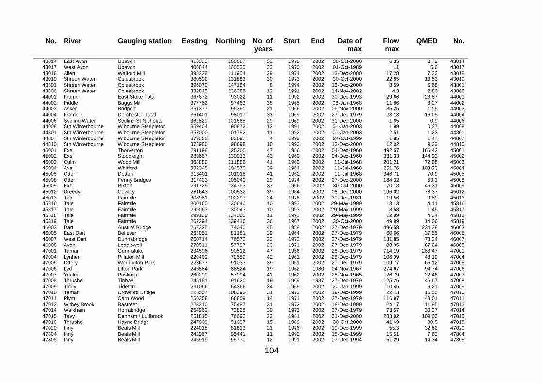
104
No. River Gauging station Easting Northing No. of years
Start End Date of max
Flow max
QMED No.
43014 East Avon Upavon 416333 160687 32 1970 2002 30-Oct-2000 6.35 3.79 43014 43017 West Avon Upavon 406844 160525 33 1970 2002 01-Oct-1989 11 5.6 43017 43018 Allen Walford Mill 398328 111954 29 1974 2002 13-Dec-2000 17.28 7.33 43018 43019 Shreen Water Colesbrook 380592 131883 30 1973 2002 30-Oct-2000 22.85 13.53 43019 43801 Shreen Water Colesbrook 396070 147184 8 1994 2002 13-Dec-2000 8.59 5.68 43801 43806 Shreen Water Colesbrook 382845 136388 12 1991 2002 14-Nov-2002 4.3 2.86 43806 44001 Frome East Stoke Total 367872 93022 11 1992 2002 30-Dec-1993 29.66 23.87 44001 44002 Piddle Baggs Mill 377762 97463 38 1965 2002 08-Jan-1968 11.86 8.27 44002 44003 Asker Bridport 351377 95390 21 1966 2002 05-Nov-2000 35.25 12.5 44003 44004 Frome Dorchester Total 361401 98017 33 1969 2002 27-Dec-1979 23.13 16.05 44004 44006 Sydling Water Sydling St Nicholas 362829 101665 29 1969 2002 31-Dec-2000 1.65 0.9 44006 44008 Sth Winterbourne W'bourne Steepleton 359404 90873 12 1991 2002 01-Jan-2003 1.99 0.37 44008 44801 Sth Winterbourne W'bourne Steepleton 352000 101792 11 1992 2002 01-Jan-2003 2.51 1.23 44801 44807 Sth Winterbourne W'bourne Steepleton 379332 82697 4 1999 2002 24-Oct-1999 1.85 1.47 44807 44810 Sth Winterbourne W'bourne Steepleton 373980 98698 10 1993 2002 13-Dec-2000 12.02 9.33 44810 45001 Exe Thorverton 291198 125205 47 1956 2002 04-Dec-1960 492.57 166.42 45001 45002 Exe Stoodleigh 289667 130913 43 1960 2002 04-Dec-1960 331.33 144.93 45002 45003 Culm Wood Mill 308880 111882 41 1962 2002 11-Jul-1968 201.21 72.08 45003 45004 Axe Whitford 332345 104570 39 1964 2002 11-Jul-1968 251.76 103.23 45004 45005 Otter Dotton 313401 101018 41 1962 2002 11-Jul-1968 346.71 70.9 45005 45008 Otter Fenny Bridges 317423 105040 29 1974 2002 07-Dec-2000 184.32 53.3 45008 45009 Exe Pixton 291729 134753 37 1966 2002 30-Oct-2000 70.18 46.31 45009 45012 Creedy Cowley 281643 100832 39 1964 2002 08-Dec-2000 196.02 78.37 45012 45013 Tale Fairmile 308981 102297 24 1978 2002 30-Dec-1981 19.56 9.89 45013 45816 Tale Fairmile 300160 130640 10 1993 2002 29-May-1999 13.13 4.11 45816 45817 Tale Fairmile 299063 130043 10 1993 2002 29-May-1999 3.58 1.45 45817 45818 Tale Fairmile 299130 134000 11 1992 2002 29-May-1999 12.99 4.34 45818 45819 Tale Fairmile 262294 139416 36 1967 2002 30-Oct-2000 49.99 14.06 45819 46003 Dart Austins Bridge 267325 74040 45 1958 2002 27-Dec-1979 496.58 234.38 46003 46005 East Dart Bellever 263051 81181 39 1964 2002 27-Dec-1979 60.66 37.56 46005 46007 West Dart Dunnabridge 260714 76572 22 1972 2002 27-Dec-1979 131.85 73.24 46007 46008 Avon Loddiswell 270511 57787 23 1971 2002 27-Dec-1979 88.95 67.24 46008 47001 Tamar Gunnislake 234596 90512 47 1956 2002 28-Dec-1979 714.19 268.47 47001 47004 Lynher Pillaton Mill 229409 72589 42 1961 2002 28-Dec-1979 106.99 48.19 47004 47005 Ottery Werrington Park 223677 91033 39 1961 2002 27-Dec-1979 109.77 65.12 47005 47006 Lyd Lifton Park 246584 88524 19 1962 1980 04-Nov-1967 274.67 94.74 47006 47007 Yealm Puslinch 260299 57994 41 1962 2002 28-Nov-1965 26.79 22.46 47007 47008 Thrushel Tinhay 245181 91620 19 1969 1987 27-Dec-1979 125.26 46.67 47008 47009 Tiddy Tideford 231066 64366 34 1969 2002 20-Jan-1999 10.45 6.21 47009 47010 Tamar Crowford Bridge 228557 108393 31 1972 2002 19-Dec-1999 22.73 16.55 47010 47011 Plym Carn Wood 256358 66809 14 1971 2002 27-Dec-1979 116.97 48.01 47011 47013 Withey Brook Bastreet 223310 75487 31 1972 2002 18-Dec-1999 24.17 11.95 47013 47014 Walkham Horrabridge 254962 73828 30 1973 2002 27-Dec-1979 73.57 30.27 47014 47015 Tavy Denham / Ludbrook 251815 76692 22 1981 2002 31-Dec-2000 283.92 109.03 47015 47018 Thrushel Hayne Bridge 247809 91097 15 1988 2002 30-Oct-2000 41.69 30.5 47018 47020 Inny Beals Mill 224015 81813 21 1976 2002 19-Dec-1999 55.3 32.62 47020 47804 Inny Beals Mill 242967 95441 11 1992 2002 18-Dec-1999 15.51 7.63 47804 47805 Inny Beals Mill 245919 95770 12 1991 2002 07-Dec-1994 51.29 14.34 47805

105
No. River Gauging station Easting Northing No. of years
Start End Date of max
Flow max
QMED No.
48001 Fowey Trekeivesteps 220765 74772 34 1969 2002 18-Dec-1999 43.2 16.97 48001 48003 Fal Tregony 194928 54536 40 1961 2002 28-Dec-1979 22.93 12 48003 48004 Warleggan Trengoffe 215277 71462 34 1969 2002 27-Dec-1979 23.64 8.91 48004 48006 Cober Helston 167298 32352 21 1968 1988 28-Dec-1979 11.94 5.53 48006 48007 Kennal Ponsanooth 172159 36762 35 1968 2002 01-Jan-2003 7.97 4.08 48007 48009 St Neot Craigshill Wood 218187 71271 12 1971 1982 27-Dec-1979 21.11 8.47 48009 48010 Seaton Trebrownbridge 227802 64417 31 1972 2002 20-Jan-1999 15.06 6.96 48010 48011 Fowey Restormel 216553 69916 18 1985 2002 19-Dec-1999 108.08 46.54 48011 48801 Fowey Restormel 168391 33697 16 1987 2002 28-Jan-1988 7.48 2.86 48801 48802 Fowey Restormel 174808 42128 9 1991 1999 18-Dec-1999 19.67 9.77 48802 48803 Fowey Restormel 173849 42260 9 1994 2002 01-Jan-2003 10.22 5.51 48803 49001 Camel Denby 207824 73231 39 1964 2002 12-Jun-1993 306.4 71.15 49001 49002 Hayle St Erth 159925 32469 46 1957 2002 01-Jan-1963 15 4.4 49002 49003 De Lank De Lank 215420 78115 37 1966 2002 21-Sep-1980 36.44 12.93 49003 49004 Gannel Gwills 186166 57381 34 1969 2002 07-Dec-2000 27.39 13.65 49004 50001 Taw Umberleigh 272169 117345 45 1958 2002 30-Oct-2000 618.24 222.45 50001 50002 Torridge Torrington 248590 107223 42 1960 2002 28-Dec-1979 516.58 230.04 50002 50005 West Okement Vellake 258022 87659 36 1967 2002 17-May-1971 53.17 21.32 50005 50006 Mole Woodleigh 274173 128743 38 1965 2002 31-Oct-1998 189.85 112.28 50006 50007 Taw Taw Bridge 264734 97339 30 1973 2002 30-Oct-2000 50.52 29.7 50007 50008 Lew Gribbleford Bridge 250125 98332 15 1988 2002 18-Dec-1999 110.34 59.64 50008 50009 Lew Norley Bridge 247497 98926 15 1988 2002 18-Dec-1999 24.68 18.89 50009 50010 Torridge Rockhay Bridge 238420 112315 15 1988 2002 19-Dec-1999 124.71 102.61 50010 50011 Okement Jacobstowe 258914 93284 20 1973 2002 27-Dec-1979 169.99 59.18 50011 50012 Yeo Veraby 282141 128002 33 1968 2002 31-Oct-1998 25.23 19.11 50012 50801 Yeo Parkham 237300 122071 32 1969 2002 27-Dec-1979 9.44 5.98 50801 51001 Doniford Stream Swill Bridge 309710 137415 37 1966 2002 10-Jul-1968 56.9 12.25 51001 51002 Horner Water West Luccombe 287466 143161 22 1973 2002 30-Oct-2000 40.8 11.6 51002 51003 Washford Beggearn Huish 300447 136965 36 1966 2002 26-May-1983 27.38 6.8 51003 52003 Halsewater Halsewater 315396 130295 42 1961 2002 09-Feb-1974 17.81 12.24 52003 52004 Isle Ashford Mill 334328 113224 40 1962 2002 30-Oct-2000 39.9 27.19 52004 52005 Tone Bishops Hull 310309 124174 42 1961 2002 30-Oct-2000 79.69 43.72 52005 52006 Yeo Pen Mill 359794 112721 41 1962 2002 15-Feb-1963 149.82 50.31 52006 52007 Parrett Chiselborough 347217 110232 37 1966 2002 30-May-1979 173.1 31.35 52007 52010 Brue Lovington 367131 135772 39 1964 2002 30-May-1979 141.57 36.28 52010 52011 Cary Somerton 355533 128169 38 1965 2002 01-Jun-1979 13.66 9.62 52011 52014 Tone Greenham 304516 127449 37 1966 2002 07-Dec-2000 26.75 13.62 52014 52015 Land Yeo Wraxall Bridge 351546 169292 24 1970 2002 16-Jul-1994 7.61 3.38 52015 52016 Currypool Stream Currypool Farm 318469 137311 33 1970 2002 01-Dec-1976 7.7 2.67 52016 52025 Hillfarrance Milverton 308310 128522 11 1992 2002 07-Dec-2000 11.34 7.63 52025 53002 Semington Brook Semington 397337 157744 27 1973 2002 14-Feb-1974 19.34 14.18 53002 53004 Chew Compton Dando 357940 160244 44 1958 2002 10-Jul-1968 226.48 18.83 53004 53007 Frome(Somerset) Tellisford 373521 146516 42 1961 2002 11-Jul-1968 113.24 57.87 53007 53008 Avon Great Somerford 388259 186712 40 1963 2002 11-Jul-1968 108.25 36.74 53008 53013 Marden Stanley 401470 172405 34 1969 2002 30-Oct-2000 43.31 15.38 53013 53017 Boyd Bitton 371777 175065 30 1973 2002 30-May-1979 27.67 12.83 53017 53018 Avon Bathford 385923 166414 34 1969 2002 30-Oct-2000 272.66 171.2 53018 53025 Mells Vallis 367966 146969 24 1979 2002 07-Oct-1993 40.27 21.54 53025

106
No. River Gauging station Easting Northing No. of years
Start End Date of max
Flow max
QMED No.
53028 By Brook Middlehill 380982 174546 22 1981 2002 02-Jan-2003 13.78 10.69 53028 54001 Severn Bewdley 336743 309876 80 1923 2002 21-Mar-1947 533.48 330.72 54001 54005 Severn Montford 310947 306938 50 1952 2002 01-Nov-2000 473.42 284.16 54005 54008 Teme Tenbury 340470 281430 47 1956 2002 03-Dec-1960 240.6 139.08 54008 54012 Tern Walcot 363754 325596 44 1959 2002 29-Jan-1990 60.02 37.6 54012 54014 Severn Abermule 300201 289855 43 1960 2002 05-Dec-1960 581.41 191.49 54014 54016 Roden Rodington 351699 328761 42 1961 2002 03-Jul-1968 28.15 14.41 54016 54018 Rea Brook Hookagate 336296 305670 41 1962 2002 06-Nov-2000 45.11 22.65 54018 54020 Perry Yeaton 337381 328873 40 1963 2002 08-Feb-1990 17.65 10.74 54020 54022 Severn Plynlimon flume 283246 288071 52 1951 2002 15-Aug-1977 32.22 13.77 54022 54025 Dulas Rhos-y-pentref 296856 278995 34 1969 2002 27-Oct-1998 46.94 23.16 54025 54028 Vyrnwy Llanymynech 307738 318661 33 1969 2002 11-Feb-2002 486.37 267.42 54028 54029 Teme Knightsford Bridge 346634 279096 33 1970 2002 28-Dec-1979 247.04 168.47 54029 54034 Dowles Brook Oak Cottage 372015 276775 32 1971 2002 10-Jun-1993 21.59 9.55 54034 54036 Isbourne Hinton on the Green 403964 231915 30 1972 2002 09-Apr-1998 37.97 13.99 54036 54038 Tanat Llanyblodwel 312711 327199 31 1972 2002 06-Nov-2000 152.09 77.14 54038 54040 Meese Tibberton 375818 322857 30 1973 2002 06-Nov-2000 9.58 5.02 54040 54041 Tern Eaton On Tern 367078 333733 31 1972 2002 07-Nov-2000 23.07 11.11 54041 54044 Tern Ternhill 372032 336285 31 1972 2002 06-Nov-2000 18.41 4.85 54044 54102 Avon Lilbourne 462407 279063 24 1974 2002 09-Apr-1998 33.15 16.46 54102 54106 Stour Shipston 424857 236671 17 1986 2002 09-Apr-1998 91.34 20.74 54106 55002 Wye Belmont 306152 255938 95 1908 2002 28-Oct-1998 607.77 380.8 55002 55003 Lugg Lugwardine 338685 257804 33 1964 2002 04-Feb-2002 60.86 44.48 55003 55004 Irfon Abernant 284965 252743 45 1937 1981 06-Aug-1973 120.41 56.54 55004 55005 Wye Rhayader 291753 277164 31 1938 1968 13-Dec-1964 279.13 115.32 55005 55007 Wye Erwood 298496 263086 64 1938 2002 02-Dec-1960 1228.83 556.22 55007 55011 Ithon Llandewi 309350 277914 15 1959 1980 03-Dec-1960 74 53.51 55011 55012 Irfon Cilmery 289393 250197 35 1966 2002 23-Oct-1998 397.74 170.27 55012 55013 Arrow Titley Mill 323594 254543 35 1966 2002 10-Jan-1986 57.66 27.25 55013 55014 Lugg Byton 324892 265277 35 1966 2002 28-Oct-1998 86.85 30.05 55014 55021 Lugg Butts Bridge 334076 264541 32 1969 2002 28-Jan-1990 64.7 44.81 55021 55022 Trothy Mitchel Troy 341042 214581 25 1970 2002 27-Dec-1979 49.1 38.28 55022 55023 Wye Redbrook 326244 248366 33 1969 2002 03-Feb-2002 904.38 530.02 55023 55025 Llynfi Three Cocks 312742 232028 32 1970 2002 27-Dec-1979 198.42 48 55025 55026 Wye Ddol Farm 292074 276803 33 1969 2001 06-Aug-1973 215.51 114.79 55026 55029 Monnow Grosmont 334942 231598 30 1973 2002 09-Apr-1998 221.91 157.37 55029 56001 Usk Chain Bridge 308051 225004 46 1957 2002 27-Dec-1979 945 387.19 56001 56003 Honddu The Forge Brecon 302453 237135 21 1963 1983 27-Dec-1979 73.04 23.46 56003 56004 Usk Llandetty 297278 229567 38 1965 2002 27-Dec-1979 774.24 328.63 56004 56006 Usk Trallong 288960 227656 38 1963 2002 23-Oct-1998 383.99 155.41 56006 56007 Senni Pont Hen Hafod 292742 221883 35 1968 2002 22-Oct-1998 53.13 27.46 56007 56013 Yscir Pontaryscir 297621 238443 31 1972 2002 06-Oct-1985 96.01 35.81 56013 57015 Taff Merthyr Tydfil 302335 214033 25 1978 2002 27-Dec-1979 313.3 93.56 57015 58002 Neath Resolven 290201 210206 42 1960 2002 16-Oct-1967 411.25 197.03 58002 58006 Mellte Pontneddfechan 294644 214977 32 1971 2002 23-Oct-1998 176.12 89.2 58006 58010 Hepste Esgair Carnau 297141 216070 18 1975 2001 22-Oct-1998 17.18 12.52 58010 58012 Afan Marcroft Weir 284377 196842 25 1978 2002 27-Dec-1979 176.79 101.74 58012 59001 Tawe Ynystanglws 277704 212026 38 1957 2002 23-Oct-1998 456.58 258.47 59001

107
No. River Gauging station Easting Northing No. of years
Start End Date of max
Flow max
QMED No.
59002 Loughor Tir-y-dail 261859 216026 36 1967 2002 26-Dec-1979 130 64.85 59002 60001 Loughor Tir-y-dail 269002 235626 29 1958 2002 27-Dec-1979 827.74 360.98 60001 60002 Cothi Felin Mynachdy 260063 237727 43 1960 2002 18-Oct-1987 498.42 156.66 60002 60003 Taf Clog-y-Fran 218991 222325 39 1964 2002 25-Aug-1986 86.39 59.77 60003 60005 Bran Llandovery 281412 241032 6 1997 2002 23-Oct-1998 51.5 41.05 60005 60006 Gwili Glangwili 240908 229292 35 1968 2002 24-Oct-1998 197.46 91.15 60006 60010 Tywi Nantgaredig 268978 235608 45 1958 2002 19-Oct-1987 890.79 308.84 60010 60013 Cothi Pont Ynys Brechfa 262036 239779 10 1971 1980 27-Dec-1979 244.1 122.9 60013 61001 Western Cleddau Prendergast Mill 195048 226904 42 1961 2002 18-Oct-1987 127.12 51.81 61001 61002 Eastern Cleddau Canaston Bridge 208851 224685 44 1959 2002 25-Aug-1986 143.21 85.97 61002 62001 Teifi Glan Teifi 248986 248171 44 1959 2002 19-Oct-1987 448.83 203.2 62001 62002 Teifi Llanfair 259932 253698 12 1971 1982 27-Dec-1979 252.51 124.98 62002 63001 Ystwyth Pont Llolwyn 271615 274267 42 1961 2002 12-Dec-1964 153.06 91.88 63001 63002 Rheidol Llanbadarn Fawr 274413 283210 28 1963 2002 29-Jun-2001 468.44 95.06 63002 64001 Dyfi Dyfi Bridge 284140 306844 41 1962 2002 06-Aug-1973 405.74 309 64001 64002 Dysynni Pont-y-Garth 269100 309379 36 1967 2002 30-Oct-2000 67.13 43.66 64002 65001 Glaslyn Beddgelert 261419 351185 36 1967 2002 19-Dec-1993 140.78 88.99 65001 65004 Gwyrfai Bontnewydd 255039 356469 32 1971 2002 21-Mar-1981 46.51 20.94 65004 65005 Erch Pencaenewydd 239274 343245 31 1972 2002 21-Aug-2000 63.39 10.85 65005 65006 Seiont Peblig Mill 257847 360309 27 1975 2002 18-Oct-1987 67.06 41.72 65006 65007 Dwyfawr Garndolbenmaen 253671 345658 29 1974 2002 18-Oct-1987 81.51 38.84 65007 66001 Clwyd Pont-y-Cambwll 309229 360668 30 1973 2002 06-Nov-2000 90.92 46.22 66001 66002 Elwy Pant yr Onen 291474 365507 12 1961 1972 12-Dec-1964 152.65 65.6 66002 66004 Wheeler Bodfari 315144 371478 29 1974 2002 06-Nov-2000 6.71 3.46 66004 66005 Clwyd Ruthin Weir 309816 351808 27 1972 2002 06-Nov-2000 21.12 14.23 66005 66006 Elwy Pont-y-Gwyddel 290505 364668 29 1974 2002 14-Oct-1976 142.31 67.4 66006 66011 Conwy Cwm Llanerch 278217 352151 38 1964 2002 11-Feb-2002 499.96 377.02 66011 67003 Brenig Llyn Brenig outflow 297273 356836 10 1964 1973 31-Jul-1972 28.82 15.28 67003 67005 Ceiriog Brynkinalt Weir 317503 336107 45 1952 2002 06-Nov-2000 66.82 29.92 67005 67006 Alwen Druid 296649 349512 43 1960 2002 12-Dec-1964 187.97 72.38 67006 67008 Alyn Pont-y-Capel 323018 359064 38 1965 2002 07-Nov-2000 58.93 22.15 67008 67009 Alyn Rhydymwyn 319019 357784 47 1956 2002 06-Nov-2000 36.33 8.62 67009 67010 Gelyn Cynefail 283514 343508 30 1966 2002 03-Jul-2001 30.08 16.36 67010 67013 Hirnant Plas Rhiwedog 296006 331068 12 1967 1978 19-Oct-1971 37.37 24.08 67013 67015 Dee Manley Hall 303096 340023 29 1974 2002 30-Oct-2000 440.57 218.11 67015 67019 Tryweryn Weir X 286121 340437 4 1960 1963 04-Dec-1960 112.7 84.19 67019 67020 Dee Chester Weir 317403 345370 75 1894 1968 09-Feb-1946 455.76 189.65 67020 68001 Weaver Ashbrook 365235 350689 66 1937 2002 08-Feb-1946 142.89 46.68 68001 68005 Weaver Audlem 359817 344402 34 1969 2002 06-Nov-2000 34.48 10.84 68005 68006 Dane Hulme Walfield 394080 365348 30 1953 1984 08-Sep-1965 113.48 53.48 68006 68007 Wincham Brook Lostock Gralam 375827 376264 41 1960 2002 03-Feb-1994 30.76 19.72 68007 68011 Arley Brook Gore Farm 366591 381600 9 1973 1981 18-Nov-1981 11.41 6.11 68011 68020 Gowy Bridge Trafford 351374 364258 24 1979 2002 06-Nov-2000 20.77 15.16 68020 68044 Dane Hugbridge 398633 367268 10 1993 2002 23-Oct-1998 177.12 46.63 68044 69017 Goyt Marple Bridge 402590 382527 33 1969 2002 16-Jul-1973 165.54 48.53 69017 71006 Ribble Henthorn 380310 457753 35 1968 2002 31-Oct-2000 494 252.38 71006 71008 Hodder Hodder Place 366843 450185 34 1969 2002 23-Oct-1980 488.14 220.16 71008 71011 Ribble Arnford 381225 469050 33 1970 2002 01-Feb-1995 149.09 115.77 71011

108
No. River Gauging station Easting Northing No. of years
Start End Date of max
Flow max
QMED No.
72002 Wyre St Michaels 354179 445967 41 1962 2002 09-Dec-1983 190.44 148.86 72002 72004 Lune Caton 366470 482803 35 1968 2002 31-Jan-1995 1181.77 606.74 72004 72005 Lune Killington New Bridge 362069 503090 32 1969 2002 06-Jan-1999 389.67 225.68 72005 72006 Lune Kirkby Lonsdale 366219 495009 16 1968 1983 02-Jan-1982 579.46 441.99 72006 72007 Brock U/S A6 356440 444787 25 1978 2002 22-Aug-1987 63.53 28.01 72007 72011 Rawthey Brigg Flatts 372441 490983 35 1968 2002 31-Jan-1995 538.65 283.26 72011 72014 Conder Galgate 351620 459069 36 1966 2002 09-Dec-1983 27.41 15.57 72014 72015 Lune Lunes Bridge 363046 505307 24 1979 2002 21-Dec-1985 387.36 228.4 72015 72016 Wyre Scorton Weir 356552 454584 35 1967 2002 22-Nov-1980 150.07 87.36 72016 73002 Crake Low Nibthwaite 329406 495149 39 1962 2002 04-Jan-1982 32.61 19.29 73002 73003 Kent Burneside 346201 501646 18 1981 1999 03-Jan-1982 89.01 65.83 73003 73005 Kent Sedgwick 350609 499239 35 1968 2002 12-Jun-1971 316.07 144.79 73005 73006 Cunsey Beck Eel House Bridge 335298 497431 30 1970 2002 04-Jan-1982 14.29 7.76 73006 73008 Bela Beetham 355394 484836 34 1969 2002 06-Jan-1999 80.07 36.57 73008 73009 Sprint Sprint Mill 349722 503242 34 1969 2002 21-Dec-1985 68.7 37.93 73009 73010 Leven Newby Bridge FMS 335814 501830 59 1938 2002 02-Dec-1954 135.26 72.56 73010 73011 Mint Mint Bridge 355566 498624 34 1969 2002 06-Jan-1999 108.37 53.67 73011 73012 Mint Mint Bridge 350452 500547 29 1974 2002 21-Dec-1985 198.69 124.52 73012 74001 Duddon Duddon Hall 321459 496418 35 1967 2002 03-Aug-1998 200.67 129.37 74001 74002 Irt Galesyke 317603 508084 34 1968 2002 06-Dec-1999 41.95 20.66 74002 74003 Ehen Bleach Green 314176 513743 30 1973 2002 24-Oct-1977 49.88 33.31 74003 74005 Ehen Braystones 307113 515094 29 1974 2002 31-Oct-1977 110.74 74.32 74005 74006 Calder Calder Hall 308073 509763 30 1973 2002 03-Aug-1998 108.08 42.05 74006 74007 Esk Cropple How 319331 501761 29 1974 2002 14-Nov-1980 127.4 102.62 74007 74008 Duddon Ulpha 323909 499065 30 1973 2002 03-Aug-1998 94.77 68.61 74008 75002 Derwent Camerton 321058 523737 43 1960 2002 09-Oct-1967 288.15 202.27 75002 75003 Derwent Ouse Bridge 327778 521979 36 1967 2002 05-Jan-1982 125.22 97.33 75003 75004 Cocker Southwaite Bridge 316121 520975 37 1966 2002 31-Oct-1977 80.88 46.59 75004 75005 Derwent Portinscale 330425 519655 31 1972 2002 31-Jan-1995 130.34 98.98 75005 75007 Glenderamackin Threlkeld 335872 526349 28 1969 2002 18-Oct-1987 83.1 60.72 75007 75009 Greta Low Briery 333182 522356 32 1971 2002 21-Dec-1985 197.02 103.97 75009 75017 Ellen Bullgill 319601 538599 27 1976 2002 05-Jan-1999 41.04 33.89 75017 76001 Haweswater Beck Burnbanks 347035 513023 25 1978 2002 04-Feb-1990 31.44 12.81 76001 76002 Eden Warwick Bridge 360654 522445 39 1959 1997 23-Mar-1968 860 397.38 76002 76003 Eamont Udford 346478 519218 42 1961 2002 24-Mar-1968 259.46 174.1 76003 76004 Lowther Eamont Bridge 350892 515622 41 1962 2002 23-Mar-1968 191.93 95.44 76004 76005 Eden Temple Sowerby 371161 515038 39 1964 2002 24-Mar-1968 347.92 244.46 76005 76007 Eden Sheepmount 355830 534240 39 1966 2004 08-Jan-2005 1520 610.75 76007 76008 Irthing Greenholme 359554 566485 36 1967 2002 06-Jan-1999 264.92 132.15 76008 76010 Petteril Harraby Green 346101 539276 33 1970 2002 28-Mar-1987 58.46 29.08 76010 76011 Coal Burn Coalburn 369386 578507 26 1966 2002 30-Aug-1975 6 1.79 76011 76014 Eden Kirkby Stephen 378419 503113 32 1971 2002 25-Nov-1979 129.62 83.06 76014 76015 Eamont Pooley Bridge 340740 517213 27 1976 2002 10-Mar-1989 74.16 59.1 76015 76806 Eamont Pooley Bridge 379229 508221 5 2000 2004 07-Jan-2005 277 164.19 76806 76809 Eamont Pooley Bridge 336376 538876 8 1997 2004 08-Jan-2005 253 139.6 76809 76810 Eamont Pooley Bridge 360686 522369 46 1959 2004 08-Jan-2005 935 405.06 76810 76811 Eamont Pooley Bridge 341782 525858 8 1997 2004 30-Jul-2002 73.4 31.25 76811 77002 Esk Canonbie 331203 593560 41 1962 2002 09-Oct-1967 570.8 346.01 77002

109
No. River Gauging station Easting Northing No. of years
Start End Date of max
Flow max
QMED No.
77003 Liddel Water Rowanburnfoot 350113 591271 29 1974 2002 17-Feb-1997 418.16 296.22 77003 78003 Annan Brydekirk 310271 593596 36 1967 2002 31-Oct-1977 486.83 314.29 78003 78004 Kinnel Water Redhall 304389 597392 37 1966 2002 30-Oct-1977 116.94 75.68 78004 78005 Kinnel Water Bridgemuir 301516 593948 24 1979 2002 21-Sep-1985 151.95 121.37 78005 79002 Nith Friars Carse 276757 605289 46 1957 2002 16-Jan-1962 908.37 443.69 79002 79003 Nith Hall Bridge 260365 610481 44 1959 2002 15-Jan-1962 219.76 71.13 79003 79004 Scar Water Capenoch 276657 598774 40 1963 2002 19-Dec-1982 192.58 132.89 79004 79005 Cluden Water Fiddlers Ford 279568 586238 40 1963 2002 31-Oct-1977 194.44 105.83 79005 79006 Nith Drumlanrig 272065 610779 36 1967 2002 30-Oct-1977 530.35 341.65 79006 80001 Urr Dalbeattie 277424 573857 40 1963 2002 21-Oct-1998 148.8 81.37 80001 81002 Cree Newton Stewart 237614 579409 40 1963 2002 25-Oct-2000 375.05 227.93 81002 81003 Luce Airyhemming 216030 569848 37 1966 2002 12-Aug-1987 295.46 163.32 81003 82001 Girvan Robstone 234068 602995 40 1963 2002 19-Dec-1982 152.74 89.27 82001 82003 Stinchar Balnowlart 224449 587731 30 1972 2002 19-Dec-1982 279.02 200.68 82003 83003 Ayr Catrine 265666 627979 33 1970 2002 10-Dec-1994 213.48 103.42 83003 83005 Irvine Shewalton 249486 638573 27 1971 2002 11-Dec-1994 398.9 212.66 83005 83006 Ayr Mainholm 256485 622724 28 1975 2002 02-Jan-1981 459.39 248.6 83006 83802 Ayr Mainholm 252528 636317 88 1913 2002 11-Dec-1994 288.71 74.7 83802 84002 Calder Muirshiel 228550 664723 21 1951 1972 09-Sep-1962 35.77 16.31 84002 84003 Clyde Hazelbank 293281 631849 48 1955 2002 12-Dec-1994 567.74 275.63 84003 84004 Clyde Sills of Clyde 295915 628161 48 1955 2002 16-Jan-1962 411.02 195.3 84004 84005 Clyde Blairston 286797 637116 47 1955 2002 12-Dec-1994 830.11 375.88 84005 84009 Nethan Kirkmuirhill 278224 637191 33 1966 2002 30-Oct-1977 80.5 35.56 84009 84011 Gryfe Craigend 232559 668504 40 1963 2002 03-Dec-1999 142.03 72.58 84011 84014 Avon Water Fairholm 268831 641740 39 1964 2002 13-Aug-1966 409.73 164.55 84014 84017 Black Cart Water Milliken Park 234786 659866 35 1968 2002 11-Dec-1994 110.14 34.82 84017 84018 Clyde Tulliford Mill 293415 628983 35 1968 2002 12-Dec-1994 575.32 247.61 84018 84020 Glazert Water Milton of Campsie 261408 679737 34 1968 2002 30-Jul-2002 90.88 56.94 84020 85001 Leven Linnbrane 240563 696549 40 1963 2002 11-Mar-1990 203.58 124.54 85001 85002 Endrick Water Gaidrew 255288 685415 40 1963 2002 01-Oct-1985 142.37 117.69 85002 85003 Falloch Glen Falloch 232804 722140 32 1971 2002 22-Dec-1991 217.06 184.25 85003 86001 Little Eachaig Dalinlongart 211516 681123 36 1967 2002 03-Nov-1979 89.83 43.46 86001 86002 Eachaig Eckford 212329 694237 19 1968 1990 10-Mar-1990 113.08 80.98 86002 89804 Eachaig Eckford 218044 733253 26 1977 2002 06-Dec-1999 75.12 58.7 89804 91802 Allt Leachdach intake 226882 776150 34 1939 1973 25-May-1953 13.3 6.35 91802 93001 Carron New Kelso 202131 848740 24 1979 2002 02-Jan-1992 313.37 174.34 93001 94001 Ewe Poolewe 199247 866278 32 1971 2002 07-Feb-1989 220.48 127.76 94001 95001 Inver Little Assynt 223040 922196 26 1977 2002 07-Feb-1989 59.13 38.7 95001 96001 Halladale Halladale 289289 947524 28 1975 2002 16-Aug-1990 191.16 106.89 96001 96002 Naver Apigill 260919 936914 25 1978 2002 04-Oct-1981 236.01 141.76 96002 96003 Strathy Strathy Bridge 280908 953653 18 1985 2002 09-Nov-2000 104.61 48.41 96003 96004 Strathmore Allnabad 242592 941764 16 1987 2002 06-Dec-1999 331.01 193.6 96004 97002 Thurso Halkirk 307125 945990 31 1972 2002 07-Oct-1993 179.22 98.09 97002
201002 Fairywater Dudgeon Bridge 45100 540100 32 1971 2002 19-Jan-1988 120.83 66.57 201002 201005 Camowen Camowen Terrace 69300 533200 31 1972 2002 22-Oct-1987 192.91 87.59 201005 201006 Drumragh Campsie Bridge 54500 526600 31 1972 2002 22-Oct-1987 246.12 106.76 201006 201007 Burn Dennet Burndennet 61300 565000 28 1975 2002 22-Oct-1987 153.02 76.63 201007 201008 Derg Castlederg 27500 547900 28 1975 2002 21-Sep-1985 244.92 200.57 201008

110
No. River Gauging station Easting Northing No. of years
Start End Date of max
Flow max
QMED No.
201009 Owenkillew Crosh 72100 550500 24 1979 2002 21-Oct-1987 508.06 286.3 201009 201010 Mourne Drumnabuoy House 54700 542000 21 1982 2002 22-Oct-1987 1063.89 593.36 201010 202001 Roe Ardnargle 86100 573500 28 1975 2002 03-Oct-1981 181.79 146.18 202001 202002 Faughan Drumahoe 70300 570100 27 1976 2002 21-Oct-1987 253.44 140.71 202002 203010 Blackwater Maydown Bridge 77000 507400 33 1970 2002 23-Oct-1987 156.99 109.25 203010 203011 Maine Dromona 125400 573800 31 1969 2002 15-Nov-2002 85.94 59.64 203011 203012 Ballinderry Ballinderry Bridge 91100 538000 34 1969 2002 22-Oct-1987 208.33 131.82 203012 203018 Six-Mile Water Antrim 139900 545000 33 1970 2002 21-Oct-1987 163.53 81.84 203018 203019 Claudy Glenone Bridge 102600 564500 32 1971 2002 23-Oct-1980 59.87 34.35 203019 203020 Moyola Moyola New Bridge 95400 554600 31 1971 2002 19-Jan-1988 155.69 113.57 203020 203022 Blackwater Derrymeen Bridge 64600 515200 24 1979 2002 22-Oct-1987 90.1 50.75 203022 203024 Cusher Gamble's Bridge 108100 494600 32 1971 2002 21-Oct-1987 73.46 47 203024 203026 Glenavy Glenavy 133400 529000 30 1971 2000 21-Oct-1987 28.72 16.29 203026 203027 Braid Ballee 133500 564700 31 1972 2002 16-Nov-1995 162.14 90.68 203027 203028 Agivey Whitehill 97000 574300 31 1972 2002 21-Oct-1987 144.09 62.99 203028 203033 Upper Bann Bannfield 133300 486500 28 1975 2002 14-Nov-2002 89.08 64.99 203033 203039 Clogh Tullynewey 130000 571900 22 1981 2002 15-Nov-1995 43.29 37.21 203039 203042 Crumlin Cidercourt Bridge 133600 533900 24 1979 2002 21-Oct-1987 79.45 37.71 203042 203043 Oonawater Shanmoy 83400 520300 22 1980 2002 25-Dec-1999 43.47 28.33 203043 203046 Rathmore Burn Rathmore Bridge 133300 546800 21 1982 2002 24-Dec-1999 15.65 11 203046 203049 Clady Clady Bridge 138000 536800 21 1982 2002 05-Dec-2001 35.41 22.74 203049 203093 Maine Shane's Viaduct 128800 564600 20 1983 2002 22-Oct-1987 298.16 211.53 203093 204001 Bush Seneirl Bridge 120800 590800 31 1972 2002 03-Oct-1981 93.96 62.25 204001 205005 Ravernet Ravernet 143900 515600 31 1972 2002 26-Nov-1997 32.5 14.49 205005 205008 Lagan Drumiller 137300 505200 29 1974 2002 28-Dec-1978 45.74 30.43 205008 205011 Annacloy Kilmore Bridge 148500 509400 24 1979 2002 08-Nov-2000 61.53 35.26 205011 206001 Clanrye Mountmill Bridge 123400 488200 32 1971 2002 20-Jan-1973 114.37 20.85 206001 206004 Bessbrook Carnbane 112900 486400 19 1984 2002 24-Oct-1998 11.91 9.29 206004 206006 Bessbrook Carnbane 142200 481400 48 1895 1942 24-Aug-1942 30.51 15.33 206006 236005 Colebrooke Ballindarragh Bridge 51300 508200 21 1982 2002 22-Oct-1987 155.28 106.47 236005 236007 Sillees Drumrainey Bridge 22600 515000 22 1981 2002 21-Dec-1991 37.32 24.14 236007

111
Appendix B FPEXT, FPLOC and FPDBAR values No. River Gauging station Easting Northing AREA
[km2]SAAR [mm]
BFIHOST [-]
FARL [-]
FPEXT FPLOC FPDBAR [cm]
No.
2001 Helmsdale Kilphedir 284324 929794 552.57 1117 0.324 0.858 0.0555 1.07 0.67 2001 2002 Brora Bruachrobie 274462 916259 423.73 1217 0.351 0.845 0.0554 1.023 0.706 2002 3002 Carron Sgodachail 240482 888010 236.84 1785 0.436 0.974 0.0376 0.864 0.632 3002 3003 Oykel Easter Turnaig 231271 901365 331.64 1896 0.359 0.915 0.0488 0.92 0.749 3003 4003 Alness Alness 253141 877497 202.32 1366 0.384 0.908 0.0373 0.999 0.541 4003 4005 Meig Glenmeannie 220273 850353 123.45 2147 0.389 0.918 0.0366 0.902 0.642 4005 4006 Bran Dosmucheran 212722 856678 117.54 2203 0.333 0.814 0.0479 0.861 0.717 4006 6003 Moriston Invermoriston 221387 812362 397.92 2117 0.362 0.985 0.0397 0.892 0.784 6003 6008 Enrick Mill of Tore 238353 828104 105.98 1292 0.43 0.839 0.0467 0.919 0.608 6008 7001 Findhorn Shenachie 273215 821452 415.59 1217 0.451 0.982 0.0392 0.763 0.625 7001 7002 Findhorn Forres 284034 830206 781.74 1065 0.434 0.973 0.0482 0.842 0.703 7002 7003 Lossie Sheriffmills 314502 853471 216.64 833 0.577 0.979 0.0741 0.684 0.679 7003 7004 Nairn Firhall 273722 837368 304.96 942 0.587 0.923 0.0682 0.821 0.787 7004 7005 Divie Dunphail 301689 839889 165.09 870 0.353 0.925 0.0566 0.968 0.542 7005 8001 Spey Aberlour 292139 810489 2645.6 1133 0.484 0.956 0.0526 0.976 0.873 8001 8002 Spey Kinrara 270711 793742 1008.94 1316 0.452 0.927 0.0565 0.825 0.966 8002 8004 Avon Delnashaugh 316609 817588 540.69 1108 0.451 0.989 0.0257 0.905 0.399 8004 8005 Spey Boat of Garten 275066 796799 1260.92 1277 0.47 0.917 0.0589 0.841 0.973 8005 8006 Spey Boat o Brig 294879 812741 2852.4 1119 0.485 0.959 0.0525 0.975 0.906 8006 8007 Spey Invertruim 258191 791354 401.59 1431 0.411 0.945 0.0539 0.803 0.807 8007 8008 Tromie Tromie Bridge 276489 786784 131.51 1437 0.447 0.898 0.0311 0.792 0.495 8008 8009 Dulnain Balnaan Bridge 285086 819396 272.2 1012 0.498 0.994 0.0505 0.677 0.576 8009 8010 Spey Grantown 279940 802927 1745.88 1194 0.484 0.938 0.0612 0.835 0.958 8010 8011 Livet Minmore 324546 823506 102.89 1001 0.449 1 0.0241 0.737 0.323 8011 9001 Deveron Avochie 344243 831607 444.8 988 0.505 0.998 0.0342 0.802 0.404 9001 9002 Deveron Muiresk 348674 840599 961.4 928 0.511 0.997 0.0412 0.878 0.469 9002 9003 Isla Grange 341980 850067 179.98 900 0.474 0.994 0.0401 0.664 0.416 9003 9004 Bogie Redcraig 348530 829933 182.4 955 0.567 0.998 0.0313 0.89 0.307 9004
10001 Ythan Ardlethen 381351 839185 456.97 830 0.614 0.992 0.0432 0.907 0.387 10001 10002 Ugie Inverugie 396184 850658 325.71 812 0.522 0.984 0.0751 0.797 0.613 10002 10003 Ythan Ellon 382301 837608 532.29 826 0.62 0.993 0.047 0.878 0.406 10003 11001 Don Parkhill 357673 817761 1269.46 884 0.584 0.996 0.0588 0.775 0.673 11001 11002 Don Haughton 348552 814053 792.65 916 0.573 0.997 0.0506 0.753 0.619 11002 11003 Don Bridge of Alford 339397 812892 509.54 967 0.565 0.996 0.0361 0.813 0.479 11003 11004 Urie Pitcaple 362209 828797 195.45 870 0.562 0.996 0.0458 0.896 0.411 11004 12001 Dee Woodend 325598 793481 1380.04 1108 0.506 0.976 0.0468 0.823 0.7 12001 12002 Dee Park 335381 793266 1833.26 1080 0.507 0.98 0.0483 0.838 0.688 12002 12003 Dee Polhollick 311368 790126 697.46 1231 0.459 0.986 0.0378 0.863 0.619 12003 12005 Muick Invermuick 330719 785799 109.39 1244 0.512 0.896 0.0293 0.762 0.403 12005 12006 Gairn Invergairn 325512 801212 145.91 1048 0.452 0.997 0.0294 0.878 0.395 12006 12007 Dee Mar Lodge 301326 789773 291.9 1334 0.4 0.989 0.0331 0.833 0.501 12007 12008 Feugh Heugh Head 360826 787475 232.84 1130 0.427 0.998 0.0381 0.608 0.456 12008 13001 Bervie Inverbervie 376480 778902 124.47 890 0.554 0.998 0.0594 0.822 0.541 13001

Science Report – Improving the FEH statistical procedures for flood frequency estimation 112
No. River Gauging station Easting Northing AREA [km2]
SAAR [mm]
BFIHOST [-]
FARL [-]
FPEXT FPLOC FPDBAR [cm]
No.
14001 Eden Kemback 330237 711373 308.72 800 0.609 0.992 0.1039 1.002 0.778 14001 15003 Tay Caputh 268182 753767 3211.11 1609 0.437 0.806 0.0406 0.938 0.847 15003 15006 Tay Ballathie 283585 754071 4586.97 1424 0.473 0.847 0.0534 0.811 0.915 15006 15007 Tay Pitnacree 259167 739905 1149.07 1950 0.442 0.836 0.0373 0.912 0.917 15007 15008 Dean Water Cookston 341011 746580 176.63 840 0.622 0.973 0.1267 0.832 1.007 15008 15010 Isla Wester Cardean 323994 760470 363.76 1086 0.532 0.94 0.0473 0.71 0.583 15010 15013 Almond Almondbank 288259 731392 173.32 1394 0.466 0.996 0.0309 0.732 0.474 15013 15016 Tay Kenmore 253572 733602 598.42 2129 0.423 0.76 0.0344 1.099 0.796 15016 16001 Earn Kinkell Bridge 275774 722833 584.7 1505 0.487 0.894 0.0561 0.723 0.729 16001 16003 Ruchill Water Cultybraggan 269860 716406 98.48 1900 0.428 1 0.0333 0.769 0.486 16003 16004 Earn Forteviot Bridge 280547 720580 783.72 1404 0.51 0.916 0.061 0.776 0.825 16004 17001 Carron Headswood 273125 684424 117.12 1530 0.372 0.844 0.0397 0.769 0.489 17001 19004 North Esk Dalmore Weir 319829 657686 79.86 949 0.561 0.975 0.0316 0.95 0.285 19004 19008 South Esk Prestonholm 331180 655398 113.44 859 0.592 0.888 0.0418 1.011 0.363 19008 19011 North Esk Dalkeith Palace 321728 659964 133.52 906 0.551 0.965 0.0329 0.879 0.327 19011 20001 Tyne East Linton 347341 666383 307.14 713 0.489 0.986 0.0503 0.87 0.404 20001 20002 West Peffer Burn Luffness 352595 680164 26.31 616 0.471 0.996 0.1279 0.832 0.851 20002 20003 Tyne Spilmersford 342842 663792 162.76 724 0.52 0.987 0.0452 0.826 0.337 20003 20005 Birns Water Saltoun Hall 345090 662102 92.61 762 0.536 0.989 0.0297 0.895 0.247 20005 20007 Gifford Water Lennoxlove 353773 665941 67.75 770 0.527 0.977 0.0293 0.681 0.245 20007 21001 Fruid Water Fruid 310750 616956 22.17 1699 0.392 1 0.0113 0.931 0.144 21001 21003 Tweed Peebles 314086 636304 698.01 1140 0.517 0.974 0.0505 0.854 0.615 21003 21005 Tweed Lyne Ford 310348 629329 377.16 1255 0.507 0.965 0.0481 0.789 0.622 21005 21007 Ettrick Water Lindean 330137 621040 502.73 1306 0.443 0.928 0.0386 0.767 0.651 21007 21008 Teviot Ormiston Mill 356832 614437 1121.49 937 0.458 0.987 0.0464 0.801 0.611 21008 21009 Tweed Norham 352257 629303 4398.66 955 0.495 0.981 0.0544 0.846 0.702 21009 21011 Yarrow Water Philiphaugh 327398 624661 232.41 1347 0.443 0.919 0.0267 0.727 0.454 21011 21012 Teviot Hawick 343049 607412 324.39 1149 0.429 0.993 0.0323 0.801 0.448 21012 21013 Gala Water Galashiels 341475 648495 205.45 930 0.531 0.999 0.0348 0.871 0.44 21013 21015 Leader Water Earlston 353943 650943 239.07 853 0.563 0.999 0.0338 0.793 0.416 21015 21016 Eye Water Eyemouth Mill 385382 663511 118.86 730 0.597 0.997 0.0356 0.854 0.313 21016 21017 Ettrick Water Brockhoperig 320191 610867 38.59 1740 0.421 1 0.012 0.721 0.213 21017 21019 Manor Water Cademuir 320823 631648 59.98 1344 0.482 0.997 0.0313 0.565 0.436 21019 21020 Yarrow Water Gordon Arms 322923 622849 153.94 1496 0.395 0.883 0.0187 0.651 0.307 21020 21021 Tweed Sprouston 340986 628413 3345.74 1014 0.496 0.978 0.046 0.9 0.651 21021 21022 Whiteadder Water Hutton Castle 371489 657271 502.24 814 0.518 0.981 0.047 0.75 0.459 21022 21024 Jed Water Jedburgh 365676 610828 139.27 915 0.436 0.997 0.0284 0.881 0.383 21024 21025 Ale Water Ancrum 347712 621531 173.94 926 0.391 0.948 0.0606 0.852 0.682 21025 21027 Blackadder Water Mouth Bridge 371059 650492 155.39 774 0.518 0.997 0.07 0.962 0.573 21027 21029 Tweed Glenbreck 305784 617310 34.37 1532 0.353 1 0.0212 0.794 0.316 21029 21030 Megget Water Henderland 318923 622287 55.97 1670 0.393 1 0.0085 0.702 0.211 21030 21031 Till Etal 394992 625894 634.78 827 0.504 0.992 0.0672 0.757 0.658 21031 21032 Glen Kirknewton 385595 625684 196.12 877 0.456 0.986 0.0395 0.793 0.436 21032 21034 Yarrow Water Craig Douglas 321501 621791 116.03 1555 0.39 0.847 0.016 0.694 0.268 21034 22001 Coquet Morwick 400758 603911 578.21 850 0.393 0.993 0.0403 0.787 0.496 22001 22002 Coquet Bygate 383302 611166 60.07 1020 0.413 1 0.0077 0.755 0.11 22002 22003 Usway Burn Shillmoor 388728 614173 21.87 1056 0.302 1 0.0061 0.937 0.083 22003 22004 Aln Hawkhill 410419 614239 202.93 758 0.427 0.997 0.0406 0.864 0.366 22004

113
No. River Gauging station Easting Northing AREA [km2]
SAAR [mm]
BFIHOST [-]
FARL [-]
FPEXT FPLOC FPDBAR [cm]
No.
22006 Blyth Hartford Bridge 411285 575860 273.62 696 0.333 0.99 0.1148 0.936 0.838 22006 22007 Wansbeck Mitford 404914 587654 282.03 794 0.347 0.973 0.0591 0.919 0.547 22007 22009 Coquet Rothbury 392511 606428 345.99 905 0.395 0.994 0.0359 0.62 0.464 22009 23001 Tyne Bywell 378954 572789 2172.36 1016 0.318 0.961 0.0504 0.839 0.719 23001 23002 Derwent Eddys Bridge 396338 549462 118.07 943 0.316 0.996 0.0203 0.863 0.234 23002 23003 North Tyne Reaverhill 377080 589424 1012.97 1023 0.31 0.993 0.0471 0.764 0.666 23003 23004 South Tyne Haydon Bridge 373642 554530 749.9 1147 0.298 0.989 0.044 0.817 0.608 23004 23005 North Tyne Tarset 365543 590723 283.38 1230 0.274 1 0.025 0.836 0.349 23005 23006 South Tyne Featherstone 369209 547794 322.97 1331 0.27 0.995 0.0303 0.77 0.459 23006 23007 Derwent Rowlands Gill 402780 551182 243.84 849 0.335 0.908 0.0264 0.842 0.33 23007 23008 Rede Rede Bridge 384095 596079 345.2 941 0.322 0.978 0.0409 0.818 0.529 23008 23009 South Tyne Alston 371823 540057 118.62 1522 0.266 0.999 0.0251 0.742 0.379 23009 23010 Tarset Burn Greenhaugh 376212 592868 95.57 993 0.305 1 0.0292 0.848 0.35 23010 23011 Kielder Burn Kielder 366671 598858 58.81 1199 0.273 1 0.0201 0.676 0.285 23011 23012 East Allen Wide Eals 383546 551702 88.18 1050 0.298 0.997 0.0268 0.848 0.371 23012 23013 West Allen Hindley Wrae 377486 551713 78.54 1156 0.28 0.998 0.0224 0.752 0.292 23013 23015 North Tyne Barrasford 377644 588998 1049.61 1013 0.311 0.989 0.0489 0.762 0.675 23015 24001 Wear Sunderland Bridge 404825 534972 661.04 933 0.342 0.978 0.0346 0.726 0.486 24001 24003 Wear Stanhope 388676 539354 173.41 1279 0.3 0.978 0.0195 0.739 0.346 24003 24004 Bedburn Beck Bedburn 405023 530533 74.13 895 0.362 0.999 0.0106 0.727 0.139 24004 24006 Rookhope Burn Eastgate 391865 542746 36.62 1126 0.293 0.994 0.0177 0.936 0.496 24006 24007 Browney Lanchester 411164 544143 44.59 797 0.333 1 0.0147 0.734 0.156 24007 24008 Wear Witton Park 398825 536850 455.1 1034 0.338 0.97 0.024 0.771 0.386 24008 25001 Tees Broken Scar 396415 521254 847.7 1122 0.354 0.945 0.0526 0.742 0.719 25001 25003 Trout Beck Moor House 373799 531877 11.46 1904 0.227 1 0.0412 0.709 0.661 25003 25005 Leven Leven Bridge 453156 507565 194.15 726 0.381 0.994 0.1067 0.933 0.835 25005 25006 Greta Rutherford Bridge 393998 510668 86.81 1127 0.241 0.999 0.0421 0.96 0.515 25006 25008 Tees Barnard Castle 388625 525152 510.17 1310 0.321 0.912 0.0345 0.944 0.53 25008 25009 Tees Low Moor 406923 520355 1267.1 966 0.374 0.958 0.0784 0.785 0.909 25009 25011 Langdon Beck Langdon 385506 533451 12.79 1463 0.237 1 0.0125 0.74 0.175 25011 25012 Harwood Beck Harwood 381653 533545 24.58 1577 0.261 1 0.0212 0.743 0.302 25012 25018 Tees Middleton in Teesdale 383018 529931 242.36 1532 0.283 0.939 0.0336 0.974 0.539 25018 25019 Leven Easby 460962 509663 15.07 830 0.525 1 0.0194 0.769 0.183 25019 26003 Foston Beck Foston Mill 504662 465194 59.4 698 0.88 0.987 0.1057 0.409 0.841 26003 26802 Foston Beck Foston Mill 488328 466463 15.85 757 0.959 1 0.0305 0.853 0.228 26802 26803 Foston Beck Foston Mill 498435 463033 32.43 721 0.949 1 0.0159 0.59 0.116 26803 27002 Wharfe Flint Mill Weir 408602 459310 759.03 1163 0.386 0.927 0.0532 0.772 0.807 27002 27007 Ure Westwick Lock 408676 481762 912.58 1120 0.42 0.981 0.0674 0.694 1.075 27007 27008 Swale Leckby Grange 422266 495156 1350.24 835 0.436 0.994 0.1182 0.699 1.105 27008 27009 Ouse Skelton 422906 481304 3300.8 899 0.439 0.983 0.1357 0.663 1.402 27009 27010 Hodge Beck Bransdale Weir 461816 498131 18.84 987 0.341 1 0.0094 1.047 0.131 27010 27014 Rye Little Habton 463598 488603 680.84 824 0.547 0.996 0.0923 0.462 0.867 27014 27024 Swale Richmond 397707 501071 377.97 1226 0.342 0.999 0.028 0.854 0.589 27024 27027 Wharfe Ilkley 398527 466714 445.22 1369 0.366 0.976 0.0362 0.89 0.523 27027 27034 Ure Kilgram Bridge 396729 487690 510.9 1338 0.386 0.99 0.0452 0.856 0.955 27034 27035 Aire Kildwick Bridge 393465 455405 283.47 1151 0.385 0.977 0.0734 0.791 0.844 27035 27038 Costa Beck Gatehouses 478405 486210 7.98 722 0.774 0.99 0.1253 0.383 0.486 27038 27041 Derwent Buttercrambe 476234 483445 1594.22 765 0.608 0.994 0.141 0.819 1.098 27041

Science Report – Improving the FEH statistical procedures for flood frequency estimation 114
No. River Gauging station Easting Northing AREA [km2]
SAAR [mm]
BFIHOST [-]
FARL [-]
FPEXT FPLOC FPDBAR [cm]
No.
27043 Wharfe Addingham 398150 467369 429.98 1385 0.366 0.975 0.035 0.909 0.501 27043 27051 Crimple Burn Bridge 426492 452134 8.15 855 0.309 1 0.0133 0.711 0.144 27051 27053 Nidd Birstwith 411968 468699 219.28 1218 0.357 0.913 0.0291 0.728 0.472 27053 27056 Pickering Beck Ings Bridge 482273 491124 67.62 834 0.691 1 0.0381 0.66 0.363 27056 27059 Laver Ripon 421740 473034 78.28 912 0.42 0.982 0.0451 0.766 0.459 27059 27084 Eastburn Beck Crosshills 397155 443837 41.01 1129 0.315 0.998 0.025 0.55 0.287 27084 27086 Skell Alma Weir 422502 471702 117.35 899 0.422 0.97 0.0458 0.759 0.457 27086 27087 Derwent Low Marishes 493360 484721 475.92 741 0.684 0.996 0.1874 0.65 1.313 27087 27089 Wharfe Tadcaster 410930 458204 815.36 1130 0.416 0.93 0.0576 0.753 0.857 27089 27090 Swale Catterick Bridge 401958 501699 497.61 1123 0.381 0.998 0.0383 0.746 0.668 27090 27201 Swale Catterick Bridge 395621 427036 172.96 1357 0.355 0.94 0.0233 0.977 0.372 27201 28008 Dove Rocester Weir 412867 354822 397.97 1022 0.555 0.991 0.0405 0.787 0.488 28008 28011 Derwent Matlock Bath 418165 376336 687.29 1114 0.565 0.947 0.0303 0.785 0.373 28011 28018 Dove Marston on Dove 408533 349064 883.12 936 0.528 0.976 0.0746 0.679 0.89 28018 28023 Wye Ashford 411226 374534 152.4 1165 0.678 0.976 0.0232 1.019 0.208 28023 28024 Wreake Syston Mill 476502 316705 417.01 634 0.403 0.953 0.0885 0.905 0.786 28024 28031 Manifold Ilam 407654 356758 148.45 1098 0.455 1 0.0327 0.912 0.424 28031 28033 Dove Hollinsclough 404552 368129 7.93 1346 0.403 1 0.0075 0.802 0.086 28033 28041 Hamps Waterhouses 405257 353971 36.97 1085 0.301 1 0.0326 0.663 0.39 28041 28043 Derwent Chatsworth 418886 383582 344.36 1170 0.461 0.909 0.0258 0.73 0.341 28043 28046 Dove Izaak Walton 411773 361404 85.7 1098 0.651 1 0.0265 0.944 0.287 28046 28055 Ecclesbourne Duffield 428768 349415 50.97 852 0.455 0.997 0.0262 0.631 0.272 28055 28058 Henmore Brook Ashbourne 422849 349884 38.48 895 0.448 0.977 0.0302 0.593 0.315 28058 28061 Churnet Basford Bridge 396765 356765 136.34 976 0.442 0.927 0.0527 0.788 0.581 28061 28070 Burbage Brook Burbage 426299 382091 8.45 1006 0.426 1 0.031 1.242 0.217 28070 29001 Waithe Beck Brigsley 520771 395873 108.14 691 0.883 0.961 0.0415 0.816 0.281 29001 29002 Great Eau Claythorpe Mill 536273 377820 80.4 692 0.713 0.952 0.0626 0.64 0.401 29002 29003 Lud Louth 529502 384953 55.72 698 0.82 0.958 0.0247 0.852 0.184 29003 29004 Ancholme Bishopbridge 501036 386992 59.03 615 0.558 0.996 0.2478 0.772 1.285 29004 29009 Ancholme Toft Newton 499618 385709 29.52 616 0.625 0.997 0.2063 0.731 0.959 29009 30003 Bain Fulsby Lock 526134 376051 199.42 667 0.757 0.963 0.0808 0.782 0.621 30003 30004 Lymn Partney Mill 534402 371019 60.24 686 0.568 0.979 0.0606 0.952 0.465 30004 30005 Witham Saltersford total 490684 325074 123.5 646 0.761 0.973 0.0925 1.203 0.485 30005 30011 Bain Goulceby Bridge 523650 386241 64.11 695 0.843 0.949 0.0521 1.022 0.308 30011 30014 Pointon Lode Pointon 508244 329902 10.94 591 0.338 1 0.1046 0.635 0.738 30014 30017 Witham Colsterworth 491229 320258 50.13 641 0.656 0.993 0.1238 1.166 0.675 30017 31004 Welland Tallington 483677 298564 708 632 0.476 0.925 0.0867 0.967 0.751 31004 31005 Welland Tixover 477726 293382 419.59 636 0.377 0.971 0.098 0.901 0.831 31005 31010 Chater Fosters Bridge 487563 303210 68.85 639 0.529 0.998 0.0318 0.808 0.293 31010 31023 West Glen Easton Wood 495229 325297 4.32 641 0.32 1 0.0516 0.966 0.3 31023 31025 Gwash South Arm Manton 482615 306835 23.93 663 0.306 0.995 0.0266 0.619 0.257 31025 32003 Harpers Brook Old Mill Bridge 491255 284601 70.46 622 0.415 1 0.0618 1.013 0.466 32003 33005 Bedford Ouse Thornborough Mill 467160 231972 387.74 655 0.48 0.983 0.1108 0.921 0.771 33005 33007 Nar Marham 582917 315878 147.47 683 0.803 0.926 0.1336 0.974 0.716 33007 33011 Little Ouse County Bridge Euston 599445 278215 130.1 596 0.653 0.985 0.1461 0.982 0.815 33011 33012 Kym Meagre Farm 506371 265471 137.99 585 0.309 0.992 0.1207 0.877 0.767 33012 33013 Sapiston Rectory Bridge 594868 268499 196.18 589 0.611 0.975 0.1367 1.03 0.78 33013 33018 Tove Cappenham Bridge 463136 247958 132.65 661 0.368 0.986 0.0627 0.798 0.562 33018
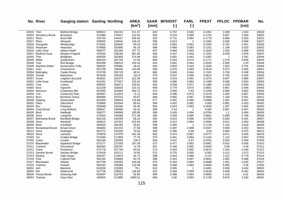
115
No. River Gauging station Easting Northing AREA [km2]
SAAR [mm]
BFIHOST [-]
FARL [-]
FPEXT FPLOC FPDBAR [cm]
No.
33019 Thet Melford Bridge 599012 291010 311.37 620 0.707 0.932 0.1901 1.039 1.024 33019 33020 Alconbury Brook Brampton 512089 276527 212.63 564 0.319 0.999 0.1742 0.807 1.065 33020 33021 Rhee Burnt Mill 534753 244427 306.06 559 0.715 0.994 0.1778 0.884 0.933 33021 33027 Rhee Wimpole 528835 243642 128.42 558 0.613 1 0.1962 0.826 0.998 33027 33029 Stringside Whitebridge 573505 305835 95.53 628 0.864 0.991 0.2263 0.782 0.951 33029 33032 Heacham Heacham 574858 333466 56.18 688 0.968 0.983 0.1161 1.199 0.533 33032 33034 Little Ouse Abbey Heath 596477 281368 707.72 607 0.694 0.959 0.1632 1.033 0.899 33034 33037 Bedford Ouse Newport Pagnell 470035 238160 801.65 648 0.437 0.943 0.1041 0.928 0.878 33037 33044 Thet Bridgham 600029 291906 274.99 620 0.681 0.942 0.1991 1 1.041 33044 33045 Wittle Quidenham 605154 287146 27.55 608 0.534 0.974 0.1771 1.079 0.859 33045 33046 Thet Red Bridge 602298 295014 143.43 624 0.581 0.944 0.2033 0.995 1.03 33046 33049 Stanford Water Buckenham Tofts 590032 295982 46.42 645 0.853 0.915 0.1649 1.063 0.791 33049 33051 Cam Chesterford 551708 236036 140.09 599 0.576 0.993 0.0518 0.973 0.406 33051 33054 Babingley Castle Rising 574758 325733 48.51 686 0.906 0.944 0.1181 0.759 0.598 33054 33055 Granta Babraham 557649 246183 101.8 579 0.637 0.999 0.0614 0.792 0.405 33055 33057 Ouzel Leighton Buzzard 493921 221073 122.39 643 0.524 0.991 0.1574 0.847 0.885 33057 33063 Little Ouse Knettishall 601051 277607 103.32 595 0.596 0.982 0.1498 0.938 0.834 33063 34001 Yare Colney 606922 304371 228.81 635 0.528 0.971 0.1386 1.028 0.849 34001 34003 Bure Ingworth 613109 333025 161.41 669 0.778 0.974 0.0851 0.967 0.495 34003 34004 Wensum Costessey Mill 597805 322666 559.72 672 0.689 0.93 0.1299 0.989 0.852 34004 34005 Tud Costessey Park 605697 311919 72.12 649 0.598 0.973 0.1578 1.094 0.867 34005 34012 Burn Burnham Overy 584689 337532 83.87 668 0.965 0.997 0.0983 1.106 0.451 34012 35008 Gipping Stowmarket 601946 259639 126.98 577 0.402 0.996 0.0988 1.062 0.567 35008 36002 Glem Glemsford 578966 252844 85.63 598 0.402 0.982 0.056 0.981 0.433 36002 36003 Box Polstead 593948 242065 56.46 566 0.554 0.993 0.0936 1.057 0.504 36003 36004 Chad Brook Long Melford 586647 250956 50.32 589 0.44 1 0.065 0.997 0.457 36004 36005 Brett Hadleigh 596377 249596 155.85 580 0.428 0.994 0.0764 1.1 0.494 36005 36006 Stour Langham 579555 245068 571.36 580 0.509 0.985 0.0861 0.848 0.768 36006 36007 Belchamp Brook Bardfield Bridge 581018 240358 58.16 560 0.523 0.996 0.0789 0.992 0.491 36007 36008 Stour Westmill 569913 247315 222.82 589 0.413 0.994 0.0684 0.912 0.582 36008 36009 Brett Cockfield 590503 255182 25.62 598 0.395 1 0.1129 1.145 0.618 36009 36010 Bumpstead Brook Broad Green 565863 241222 27.58 588 0.387 0.999 0.0447 0.905 0.352 36010 36012 Stour Kedington 567272 251505 76.64 599 0.396 0.99 0.06 0.984 0.475 36012 36015 Stour Lamarsh 576876 247076 481.29 583 0.474 0.987 0.0777 0.871 0.655 36015 37003 Ter Crabbs Bridge 573430 217809 77.76 570 0.461 0.994 0.1153 1.142 0.607 37003 37005 Colne Lexden 581429 232555 235.9 566 0.537 0.97 0.0761 0.952 0.549 37005 37010 Blackwater Appleford Bridge 575177 227559 247.09 572 0.477 0.992 0.0981 0.816 0.658 37010 37011 Chelmer Churchend 560093 228787 72.78 591 0.448 0.992 0.0595 0.99 0.46 37011 37012 Colne Poolstreet 572778 237726 64.54 574 0.403 0.992 0.0674 1.034 0.449 37012 37013 Sandon Brook Sandon Bridge 575428 201211 74.95 575 0.276 0.855 0.092 1.012 1.573 37013 37014 Roding High Ongar 558197 213815 92.74 598 0.403 0.986 0.107 1.012 0.779 37014 37016 Pant Copford Hall 562345 235668 63.78 588 0.404 0.997 0.0691 1.082 0.488 37016 37017 Blackwater Stisted 567758 232355 140.38 579 0.493 0.994 0.0688 1.001 0.535 37017 37020 Chelmer Felsted 562293 226088 132.96 588 0.468 0.982 0.0659 0.965 0.49 37020 38002 Ash Mardock 543206 222683 78.1 619 0.505 1 0.0491 0.938 0.424 38002 38004 Rib Wadesmill 537728 228623 136.69 625 0.469 0.999 0.0538 0.948 0.492 38004 38026 Pincey Brook Sheering Hall 554007 216705 52.85 599 0.388 0.984 0.0892 1.018 0.61 38026 39002 Thames Days Weir 430925 212889 3480.01 690 0.65 0.953 0.1758 0.879 1.632 39002

Science Report – Improving the FEH statistical procedures for flood frequency estimation 116
No. River Gauging station Easting Northing AREA [km2]
SAAR [mm]
BFIHOST [-]
FARL [-]
FPEXT FPLOC FPDBAR [cm]
No.
39006 Windrush Newbridge 418884 219840 361.6 744 0.79 0.951 0.075 0.589 0.647 39006 39008 Thames Eynsham 414913 204780 1626.71 730 0.686 0.946 0.1923 0.827 1.933 39008 39016 Kennet Theale 433673 170432 1037.36 758 0.766 0.965 0.0782 0.811 0.649 39016 39018 Kennet Theale 437749 192940 248.21 637 0.635 0.986 0.2001 0.862 1.157 39018 39019 Lambourn Shaw 437599 178291 235.21 736 0.839 0.979 0.034 0.88 0.231 39019 39020 Coln Bibury 405568 216076 107.29 821 0.858 0.968 0.0291 0.8 0.259 39020 39025 Enborne Brimpton 448699 160992 142.08 789 0.5 0.978 0.0755 0.79 0.731 39025 39026 Cherwell Banbury 449514 249775 204.57 664 0.41 0.95 0.1055 0.866 0.835 39026 39028 Dun Hungerford 425985 164944 100.1 786 0.768 0.988 0.0498 1.008 0.274 39028 39029 Tillingbourne Shalford 508055 146327 58.78 810 0.885 0.879 0.0289 0.664 0.291 39029 39034 Evenlode Cassington Mill 432691 223000 427.14 691 0.699 0.965 0.0682 0.996 0.541 39034 39035 Churn Cerney Wick 400043 209009 126.74 833 0.825 0.89 0.0623 0.482 0.516 39035 39036 Law Brook Albury 507366 144917 16.05 819 0.888 0.96 0.0173 0.588 0.163 39036 39037 Kennet Marlborough 410751 170291 136.48 772 0.959 1 0.0763 1.091 0.459 39037 39042 Leach Priory Mill Lechlade 415948 209471 77.57 736 0.865 0.971 0.0822 0.612 0.552 39042 39081 Ock Abingdon 437189 192523 233.6 639 0.623 0.986 0.2022 0.851 1.162 39081 40004 Rother Udiam 566051 125058 204.71 857 0.388 0.975 0.0575 0.674 0.715 40004 40005 Beult Stile Bridge 585642 142131 278.05 691 0.353 0.992 0.184 0.886 1.227 40005 40009 Teise Stone Bridge 566350 135405 134.5 812 0.443 0.904 0.0413 0.755 0.487 40009 41003 Cuckmere Sherman Bridge 556551 114104 130.45 814 0.405 0.978 0.0966 0.759 0.956 41003 41005 Ouse Gold Bridge 535445 127422 182.48 835 0.494 0.922 0.0445 0.771 0.468 41005 41011 Rother Iping Mill 477884 125009 156.9 921 0.675 0.973 0.078 0.858 0.691 41011 41014 Arun Pallingham Quay 507351 132316 382.69 805 0.39 0.958 0.0849 0.824 0.864 41014 41015 Ems Westbourne 478470 113230 57.92 899 0.904 0.976 0.0387 0.657 0.291 41015 41016 Cuckmere Cowbeech 560883 118771 19.09 855 0.471 0.966 0.0434 0.516 0.476 41016 41018 Kird Tanyards 498540 128368 67.25 820 0.36 0.961 0.1069 0.866 0.985 41018 41020 Bevern Stream Clappers Bridge 536753 115688 35.42 886 0.355 0.993 0.0757 0.953 0.688 41020 41022 Lod Halfway Bridge 491432 126898 52.44 857 0.48 0.951 0.0611 0.876 0.649 41022 41023 Lavant Graylingwell 487719 113373 86.29 922 0.935 1 0.034 0.656 0.235 41023 41025 Loxwood Stream Drungewick 498040 134412 92.96 812 0.321 0.962 0.0936 0.712 1.023 41025 41028 Chess Stream Chess Bridge 525651 115288 24.92 849 0.497 0.983 0.0971 0.722 0.779 41028 42003 Lymington Brockenhurst 426184 105415 99.67 854 0.386 0.997 0.1071 0.709 0.845 42003 42005 Wallop Brook Broughton 428891 137030 53.51 770 0.955 1 0.0537 0.951 0.266 42005 42006 Meon Mislingford 463826 120638 75.85 896 0.952 0.979 0.0488 0.907 0.359 42006 42008 Cheriton Stream Sewards Bridge 461728 127314 74.34 885 0.941 0.995 0.0403 0.824 0.259 42008 42009 Candover Stream Borough Bridge 460963 141287 72.07 819 0.951 0.93 0.0393 0.926 0.253 42009 42010 Itchen Highbridge+Allbrook 457279 132838 327.81 834 0.949 0.949 0.0513 0.8 0.373 42010 42011 Hamble Frogmill 456316 119165 55.33 838 0.746 0.991 0.0443 0.736 0.337 42011 42014 Blackwater Ower 426272 120791 102.42 837 0.479 0.979 0.0532 0.855 0.423 42014 43003 Avon East Mills 405962 140935 1459.55 807 0.894 0.985 0.0694 0.868 0.622 43003 43004 Bourne Laverstock 421744 146232 165.21 768 0.952 1 0.0561 0.918 0.358 43004 43005 Avon Amesbury 413152 155342 326.55 744 0.903 1 0.071 1.054 0.43 43005 43006 Nadder Wilton 395753 129698 215.68 875 0.763 0.976 0.0472 0.821 0.423 43006 43007 Stour Throop 385102 113186 1064.02 861 0.664 0.988 0.1124 0.921 1.024 43007 43008 Wylye South Newton 396257 142669 447.94 830 0.937 0.976 0.0518 0.887 0.366 43008 43009 Stour Hammoon 376203 119594 518.88 849 0.442 0.992 0.1227 0.851 0.953 43009 43010 Allen Loverley Mill 398756 115822 94.89 872 0.944 0.985 0.0523 0.645 0.368 43010 43012 Wylye Norton Bavant 385023 140062 114.01 925 0.885 0.975 0.0592 0.788 0.365 43012

117
No. River Gauging station Easting Northing AREA [km2]
SAAR [mm]
BFIHOST [-]
FARL [-]
FPEXT FPLOC FPDBAR [cm]
No.
43014 East Avon Upavon 416333 160687 85.83 759 0.838 1 0.1188 0.934 0.626 43014 43017 West Avon Upavon 406844 160525 84.62 744 0.872 1 0.1187 0.935 0.625 43017 43018 Allen Walford Mill 398328 111954 170.88 860 0.914 0.979 0.0675 0.712 0.452 43018 43019 Shreen Water Colesbrook 380592 131883 30.36 884 0.565 0.993 0.063 0.779 0.433 43019 43801 Shreen Water Colesbrook 396070 147184 68 807 0.974 1 0.0246 0.701 0.193 43801 43806 Shreen Water Colesbrook 382845 136388 50.04 968 0.931 1 0.0367 0.982 0.233 43806 44001 Frome East Stoke Total 367872 93022 414.4 968 0.778 0.968 0.0711 0.651 0.554 44001 44002 Piddle Baggs Mill 377762 97463 183.79 942 0.86 0.969 0.0537 0.663 0.437 44002 44003 Asker Bridport 351377 95390 48.51 924 0.696 0.994 0.0249 0.583 0.275 44003 44004 Frome Dorchester Total 361401 98017 205.67 1010 0.775 0.971 0.0348 0.66 0.305 44004 44006 Sydling Water Sydling St Nicholas 362829 101665 12.06 1030 0.879 0.944 0.0162 0.564 0.11 44006 44008 Sth Winterbourne W'bourne Steepleton 359404 90873 20.17 1012 0.811 1 0.0149 0.668 0.11 44008 44801 Sth Winterbourne W'bourne Steepleton 352000 101792 11.76 1030 0.597 0.923 0.0183 0.595 0.153 44801 44807 Sth Winterbourne W'bourne Steepleton 379332 82697 16.78 894 0.786 1 0.015 0.636 0.124 44807 44810 Sth Winterbourne W'bourne Steepleton 373980 98698 107.23 969 0.882 0.99 0.0357 0.649 0.307 44810 45001 Exe Thorverton 291198 125205 608.13 1249 0.526 0.985 0.0313 0.7 0.451 45001 45002 Exe Stoodleigh 289667 130913 420.71 1361 0.495 0.979 0.0216 0.799 0.324 45002 45003 Culm Wood Mill 308880 111882 228.88 971 0.585 0.993 0.065 0.63 0.574 45003 45004 Axe Whitford 332345 104570 288.53 994 0.498 0.996 0.0383 0.742 0.408 45004 45005 Otter Dotton 313401 101018 202.79 971 0.549 0.996 0.0502 0.746 0.504 45005 45008 Otter Fenny Bridges 317423 105040 105.29 1040 0.491 0.994 0.0361 0.701 0.363 45008 45009 Exe Pixton 291729 134753 147.85 1375 0.548 0.95 0.017 0.818 0.238 45009 45012 Creedy Cowley 281643 100832 263.63 909 0.577 0.993 0.0401 0.634 0.421 45012 45013 Tale Fairmile 308981 102297 31.4 922 0.514 0.998 0.048 0.771 0.431 45013 45816 Tale Fairmile 300160 130640 6.81 1210 0.59 1 0.0114 0.734 0.117 45816 45817 Tale Fairmile 299063 130043 1.74 1207 0.603 1 0.0172 0.718 0.141 45817 45818 Tale Fairmile 299130 134000 9.85 1270 0.578 1 0.0056 0.61 0.064 45818 45819 Tale Fairmile 262294 139416 78.06 1342 0.575 0.973 0.0113 0.782 0.144 45819 46003 Dart Austins Bridge 267325 74040 249.75 1771 0.523 0.995 0.0359 1.053 0.519 46003 46005 East Dart Bellever 263051 81181 22.27 2095 0.363 1 0.042 0.863 0.588 46005 46007 West Dart Dunnabridge 260714 76572 47.49 1987 0.367 1 0.0489 0.846 0.637 46007 46008 Avon Loddiswell 270511 57787 102.37 1549 0.554 0.986 0.0299 0.941 0.512 46008 47001 Tamar Gunnislake 234596 90512 920.16 1215 0.481 0.993 0.044 0.96 0.597 47001 47004 Lynher Pillaton Mill 229409 72589 135.29 1423 0.549 0.996 0.0339 0.987 0.457 47004 47005 Ottery Werrington Park 223677 91033 121.64 1199 0.45 0.999 0.0465 0.796 0.557 47005 47006 Lyd Lifton Park 246584 88524 220.39 1228 0.485 0.996 0.035 0.785 0.449 47006 47007 Yealm Puslinch 260299 57994 56.9 1428 0.549 0.987 0.0321 0.728 0.406 47007 47008 Thrushel Tinhay 245181 91620 112.7 1144 0.422 0.999 0.0362 0.803 0.447 47008 47009 Tiddy Tideford 231066 64366 37.37 1276 0.591 1 0.0237 0.695 0.309 47009 47010 Tamar Crowford Bridge 228557 108393 77.73 1181 0.386 0.947 0.0635 0.763 0.697 47010 47011 Plym Carn Wood 256358 66809 79.4 1618 0.481 0.95 0.0281 0.873 0.387 47011 47013 Withey Brook Bastreet 223310 75487 16.03 1684 0.367 0.998 0.0593 0.71 0.636 47013 47014 Walkham Horrabridge 254962 73828 44.31 1664 0.585 1 0.0228 0.876 0.321 47014 47015 Tavy Denham / Ludbrook 251815 76692 198.07 1555 0.553 0.999 0.0295 0.98 0.548 47015 47018 Thrushel Hayne Bridge 247809 91097 57.5 1164 0.419 0.999 0.0433 0.838 0.519 47018 47020 Inny Beals Mill 224015 81813 102.05 1429 0.576 1 0.0358 0.937 0.476 47020 47804 Inny Beals Mill 242967 95441 7.17 1150 0.398 1 0.0059 1.033 0.044 47804 47805 Inny Beals Mill 245919 95770 11.34 1188 0.411 1 0.0066 0.609 0.092 47805

Science Report – Improving the FEH statistical procedures for flood frequency estimation 118
No. River Gauging station Easting Northing AREA [km2]
SAAR [mm]
BFIHOST [-]
FARL [-]
FPEXT FPLOC FPDBAR [cm]
No.
48001 Fowey Trekeivesteps 220765 74772 36.8 1636 0.445 0.938 0.0435 0.849 0.571 48001 48003 Fal Tregony 194928 54536 89.03 1211 0.546 0.983 0.0656 1.109 0.624 48003 48004 Warleggan Trengoffe 215277 71462 25.26 1445 0.499 0.978 0.035 1.14 0.417 48004 48006 Cober Helston 167298 32352 40.83 1206 0.671 0.979 0.0337 0.879 0.291 48006 48007 Kennal Ponsanooth 172159 36762 26.83 1294 0.736 0.866 0.0258 0.946 0.196 48007 48009 St Neot Craigshill Wood 218187 71271 22.91 1512 0.463 0.982 0.0224 0.98 0.253 48009 48010 Seaton Trebrownbridge 227802 64417 38.57 1325 0.59 0.993 0.0202 0.932 0.24 48010 48011 Fowey Restormel 216553 69916 167.21 1435 0.522 0.92 0.035 1.006 0.525 48011 48801 Fowey Restormel 168391 33697 26.53 1265 0.672 0.976 0.0351 0.753 0.292 48801 48802 Fowey Restormel 174808 42128 42.69 1148 0.615 0.909 0.0165 0.722 0.168 48802 48803 Fowey Restormel 173849 42260 33.62 1161 0.623 0.984 0.0214 0.807 0.243 48803 49001 Camel Denby 207824 73231 209.94 1338 0.555 0.987 0.0338 1.142 0.402 49001 49002 Hayle St Erth 159925 32469 48.51 1076 0.642 0.977 0.0264 0.743 0.257 49002 49003 De Lank De Lank 215420 78115 21.61 1628 0.379 0.998 0.0636 0.848 0.663 49003 49004 Gannel Gwills 186166 57381 40.83 1046 0.617 0.999 0.0254 0.895 0.267 49004 50001 Taw Umberleigh 272169 117345 832.97 1153 0.472 0.997 0.0374 0.888 0.531 50001 50002 Torridge Torrington 248590 107223 664.23 1185 0.425 0.996 0.0496 0.935 0.742 50002 50005 West Okement Vellake 258022 87659 13.37 2066 0.349 0.981 0.0143 0.733 0.223 50005 50006 Mole Woodleigh 274173 128743 326.99 1306 0.502 0.999 0.0316 0.805 0.429 50006 50007 Taw Taw Bridge 264734 97339 72.16 1226 0.49 0.994 0.046 0.902 0.557 50007 50008 Lew Gribbleford Bridge 250125 98332 71.18 1192 0.406 0.999 0.0438 0.794 1.002 50008 50009 Lew Norley Bridge 247497 98926 20.16 1195 0.446 1 0.0231 0.785 0.28 50009 50010 Torridge Rockhay Bridge 238420 112315 258.42 1231 0.399 0.997 0.0487 0.894 0.66 50010 50011 Okement Jacobstowe 258914 93284 80.2 1509 0.478 0.981 0.0299 0.804 0.436 50011 50012 Yeo Veraby 282141 128002 53.88 1316 0.461 1 0.0375 0.753 0.432 50012 50801 Yeo Parkham 237300 122071 7.51 1238 0.47 1 0.0023 9.999 0.023 50801 51001 Doniford Stream Swill Bridge 309710 137415 74.22 911 0.629 0.988 0.0381 0.514 0.353 51001 51002 Horner Water West Luccombe 287466 143161 20.38 1485 0.539 0.978 0.0028 9.999 0.038 51002 51003 Washford Beggearn Huish 300447 136965 36.7 1151 0.588 0.982 0.0048 9.999 0.058 51003 52003 Halsewater Halsewater 315396 130295 88.25 851 0.625 0.991 0.0666 0.522 0.572 52003 52004 Isle Ashford Mill 334328 113224 87.41 891 0.499 0.979 0.0837 0.589 0.705 52004 52005 Tone Bishops Hull 310309 124174 203.65 964 0.562 0.977 0.0537 0.539 0.524 52005 52006 Yeo Pen Mill 359794 112721 216.18 865 0.569 0.965 0.0722 0.879 0.588 52006 52007 Parrett Chiselborough 347217 110232 74.26 886 0.537 1 0.0665 0.806 0.564 52007 52010 Brue Lovington 367131 135772 137.79 866 0.527 0.997 0.0815 0.608 0.629 52010 52011 Cary Somerton 355533 128169 84.62 715 0.532 1 0.2355 1.03 1.478 52011 52014 Tone Greenham 304516 127449 57.67 1101 0.553 0.937 0.0111 0.602 0.134 52014 52015 Land Yeo Wraxall Bridge 351546 169292 23.33 906 0.669 0.933 0.0579 0.678 0.442 52015 52016 Currypool Stream Currypool Farm 318469 137311 15.7 934 0.586 1 0.0375 0.435 0.394 52016 52025 Hillfarrance Milverton 308310 128522 27.75 1009 0.633 0.996 0.023 0.59 0.227 52025 53002 Semington Brook Semington 397337 157744 153.39 712 0.564 0.987 0.1214 0.787 0.705 53002 53004 Chew Compton Dando 357940 160244 128.9 987 0.591 0.842 0.045 0.903 0.383 53004 53007 Frome(Somerset) Tellisford 373521 146516 263.74 965 0.563 0.96 0.0545 0.899 0.506 53007 53008 Avon Great Somerford 388259 186712 305.19 804 0.622 0.988 0.0931 0.874 0.607 53008 53013 Marden Stanley 401470 172405 99.34 724 0.559 0.98 0.073 1.017 0.477 53013 53017 Boyd Bitton 371777 175065 47.71 806 0.497 0.998 0.0503 1.035 0.424 53017 53018 Avon Bathford 385923 166414 1569.29 817 0.575 0.985 0.0961 1.029 0.731 53018 53025 Mells Vallis 367966 146969 118.05 1056 0.656 0.943 0.0453 1.058 0.358 53025

119
No. River Gauging station Easting Northing AREA [km2]
SAAR [mm]
BFIHOST [-]
FARL [-]
FPEXT FPLOC FPDBAR [cm]
No.
53028 By Brook Middlehill 380982 174546 100.76 835 0.726 0.999 0.0315 1.01 0.226 53028 54001 Severn Bewdley 336743 309876 4329.83 912 0.541 0.973 0.1055 0.941 1.172 54001 54005 Severn Montford 310947 306938 2026.73 1147 0.47 0.977 0.0919 0.719 1.344 54005 54008 Teme Tenbury 340470 281430 1124.59 841 0.612 0.994 0.0635 0.85 0.662 54008 54012 Tern Walcot 363754 325596 851.65 694 0.616 0.966 0.1636 0.979 1.172 54012 54014 Severn Abermule 300201 289855 574.66 1256 0.449 0.97 0.0598 0.822 0.847 54014 54016 Roden Rodington 351699 328761 261.94 693 0.615 0.981 0.2212 1.085 1.38 54016 54018 Rea Brook Hookagate 336296 305670 173.1 757 0.508 0.991 0.0756 0.859 0.576 54018 54020 Perry Yeaton 337381 328873 188.05 739 0.654 0.954 0.19 1.02 1.427 54020 54022 Severn Plynlimon flume 283246 288071 8.69 2483 0.323 1 0.0098 0.8 0.132 54022 54025 Dulas Rhos-y-pentref 296856 278995 53.17 1268 0.439 1 0.024 0.965 0.263 54025 54028 Vyrnwy Llanymynech 307738 318661 778.96 1339 0.439 0.969 0.0519 0.817 0.814 54028 54029 Teme Knightsford Bridge 346634 279096 1483.65 818 0.6 0.994 0.0618 0.901 0.74 54029 54034 Dowles Brook Oak Cottage 372015 276775 42.1 715 0.632 0.997 0.0117 0.878 0.134 54034 54036 Isbourne Hinton on the Green 403964 231915 92.75 701 0.479 0.99 0.0694 0.596 0.543 54036 54038 Tanat Llanyblodwel 312711 327199 240.98 1274 0.476 0.996 0.0382 0.829 0.529 54038 54040 Meese Tibberton 375818 322857 159.94 700 0.588 0.931 0.1125 0.992 0.809 54040 54041 Tern Eaton On Tern 367078 333733 193.51 719 0.645 0.954 0.1198 0.9 0.999 54041 54044 Tern Ternhill 372032 336285 95.66 739 0.698 0.96 0.1004 0.861 0.812 54044 54102 Avon Lilbourne 462407 279063 109.57 668 0.354 0.906 0.0951 0.775 0.704 54102 54106 Stour Shipston 424857 236671 185.16 677 0.454 0.993 0.0417 0.764 0.374 54106 55002 Wye Belmont 306152 255938 1894.26 1230 0.472 0.967 0.0693 0.695 1.607 55002 55003 Lugg Lugwardine 338685 257804 885.11 813 0.588 0.99 0.1064 0.775 1.034 55003 55004 Irfon Abernant 284965 252743 73.06 1845 0.402 1 0.0287 0.658 0.459 55004 55005 Wye Rhayader 291753 277164 164.46 1656 0.419 0.997 0.0414 0.913 0.619 55005 55007 Wye Erwood 298496 263086 1283.4 1386 0.426 0.96 0.0412 0.894 0.612 55007 55011 Ithon Llandewi 309350 277914 110.47 1086 0.395 0.999 0.0283 0.775 0.338 55011 55012 Irfon Cilmery 289393 250197 246.4 1627 0.431 0.997 0.0418 0.789 0.611 55012 55013 Arrow Titley Mill 323594 254543 125.92 962 0.553 0.999 0.0382 0.742 0.4 55013 55014 Lugg Byton 324892 265277 202.54 977 0.593 0.996 0.0646 0.67 0.633 55014 55021 Lugg Butts Bridge 334076 264541 365.9 877 0.61 0.992 0.0902 0.658 0.812 55021 55022 Trothy Mitchel Troy 341042 214581 141.9 887 0.572 0.998 0.0451 0.909 0.445 55022 55023 Wye Redbrook 326244 248366 4016.42 1010 0.542 0.979 0.0824 0.857 1.392 55023 55025 Llynfi Three Cocks 312742 232028 131.51 999 0.576 0.95 0.0367 0.889 0.348 55025 55026 Wye Ddol Farm 292074 276803 172.17 1636 0.423 0.997 0.041 0.92 0.613 55026 55029 Monnow Grosmont 334942 231598 355.07 956 0.583 0.997 0.0723 0.788 0.745 55029 56001 Usk Chain Bridge 308051 225004 913.2 1367 0.597 0.98 0.0445 0.783 0.769 56001 56003 Honddu The Forge Brecon 302453 237135 62.5 1171 0.528 0.999 0.0268 0.907 0.325 56003 56004 Usk Llandetty 297278 229567 545.59 1478 0.547 0.974 0.037 0.865 0.547 56004 56006 Usk Trallong 288960 227656 184.74 1674 0.477 0.963 0.0365 0.865 0.511 56006 56007 Senni Pont Hen Hafod 292742 221883 19.31 1974 0.495 1 0.0432 0.776 0.573 56007 56013 Yscir Pontaryscir 297621 238443 63.26 1299 0.494 1 0.0256 0.963 0.342 56013 57015 Taff Merthyr Tydfil 302335 214033 111.18 1858 0.352 0.85 0.0273 0.807 0.374 57015 58002 Neath Resolven 290201 210206 190.8 1946 0.346 0.983 0.0428 0.831 0.637 58002 58006 Mellte Pontneddfechan 294644 214977 65.35 1981 0.322 0.975 0.0297 0.913 0.41 58006 58010 Hepste Esgair Carnau 297141 216070 10.94 2079 0.261 1 0.0397 0.917 0.557 58010 58012 Afan Marcroft Weir 284377 196842 89.42 2038 0.451 1 0.0172 0.613 0.298 58012 59001 Tawe Ynystanglws 277704 212026 227.46 1890 0.407 0.996 0.0504 0.771 0.902 59001

Science Report – Improving the FEH statistical procedures for flood frequency estimation 120
No. River Gauging station Easting Northing AREA [km2]
SAAR [mm]
BFIHOST [-]
FARL [-]
FPEXT FPLOC FPDBAR [cm]
No.
59002 Loughor Tir-y-dail 261859 216026 46.28 1500 0.467 0.998 0.0535 0.703 0.633 59002 60001 Loughor Tir-y-dail 269002 235626 1090.83 1535 0.478 0.984 0.0607 0.767 1.321 60001 60002 Cothi Felin Mynachdy 260063 237727 298.73 1551 0.5 0.997 0.0315 0.974 0.48 60002 60003 Taf Clog-y-Fran 218991 222325 216.48 1420 0.553 0.999 0.0505 0.741 0.671 60003 60005 Bran Llandovery 281412 241032 63.71 1489 0.485 0.997 0.0494 0.548 0.581 60005 60006 Gwili Glangwili 240908 229292 131.05 1603 0.536 0.999 0.0295 0.837 0.447 60006 60010 Tywi Nantgaredig 268978 235608 1092.13 1534 0.478 0.984 0.061 0.766 1.33 60010 60013 Cothi Pont Ynys Brechfa 262036 239779 243.04 1538 0.493 0.997 0.0336 0.934 0.478 60013 61001 Western Cleddau Prendergast Mill 195048 226904 197.8 1276 0.56 0.996 0.0444 0.948 0.557 61001 61002 Eastern Cleddau Canaston Bridge 208851 224685 181.9 1437 0.537 0.967 0.0414 0.83 0.55 61002 62001 Teifi Glan Teifi 248986 248171 897.26 1379 0.507 0.995 0.0485 1.168 0.757 62001 62002 Teifi Llanfair 259932 253698 517.56 1392 0.484 0.993 0.0619 1.043 0.846 62002 63001 Ystwyth Pont Llolwyn 271615 274267 174.54 1445 0.491 0.99 0.0462 0.772 0.69 63001 63002 Rheidol Llanbadarn Fawr 274413 283210 181.88 1756 0.435 0.898 0.0537 0.709 0.977 63002 64001 Dyfi Dyfi Bridge 284140 306844 464.65 1835 0.478 0.995 0.0292 0.763 0.534 64001 64002 Dysynni Pont-y-Garth 269100 309379 74.93 2166 0.448 0.951 0.0551 0.624 0.814 64002 65001 Glaslyn Beddgelert 261419 351185 67.14 2809 0.406 0.896 0.0487 0.844 1.721 65001 65004 Gwyrfai Bontnewydd 255039 356469 46.12 2153 0.412 0.862 0.0655 0.857 0.974 65004 65005 Erch Pencaenewydd 239274 343245 19.39 1477 0.439 0.991 0.0711 0.955 0.78 65005 65006 Seiont Peblig Mill 257847 360309 79.92 2258 0.499 0.85 0.0622 0.781 1.46 65006 65007 Dwyfawr Garndolbenmaen 253671 345658 51.56 2056 0.404 0.968 0.0558 0.677 0.761 65007 66001 Clwyd Pont-y-Cambwll 309229 360668 404.67 910 0.588 0.993 0.057 0.707 0.518 66001 66002 Elwy Pant yr Onen 291474 365507 218.53 1145 0.483 0.979 0.0339 0.902 0.406 66002 66004 Wheeler Bodfari 315144 371478 62.9 863 0.696 0.975 0.028 0.978 0.191 66004 66005 Clwyd Ruthin Weir 309816 351808 96.37 958 0.518 0.995 0.0371 0.733 0.348 66005 66006 Elwy Pont-y-Gwyddel 290505 364668 191.38 1185 0.476 0.98 0.0318 0.897 0.366 66006 66011 Conwy Cwm Llanerch 278217 352151 341.76 2040 0.363 0.976 0.0461 0.903 0.754 66011 67003 Brenig Llyn Brenig outflow 297273 356836 22.44 1317 0.319 0.983 0.0182 1.072 0.154 67003 67005 Ceiriog Brynkinalt Weir 317503 336107 111.76 1198 0.462 1 0.0231 0.783 0.337 67005 67006 Alwen Druid 296649 349512 185.66 1305 0.403 0.897 0.0381 0.846 0.466 67006 67008 Alyn Pont-y-Capel 323018 359064 225.76 917 0.591 0.99 0.048 0.865 0.442 67008 67009 Alyn Rhydymwyn 319019 357784 81.6 968 0.615 0.99 0.0328 1.068 0.322 67009 67010 Gelyn Cynefail 283514 343508 12.87 2000 0.251 0.969 0.0322 0.703 0.458 67010 67013 Hirnant Plas Rhiwedog 296006 331068 32.47 1756 0.415 1 0.0182 0.682 0.26 67013 67015 Dee Manley Hall 303096 340023 1008.74 1367 0.431 0.934 0.0457 0.963 0.741 67015 67019 Tryweryn Weir X 286121 340437 110.98 1840 0.312 0.982 0.0448 0.92 0.624 67019 67020 Dee Chester Weir 317403 345370 1800.92 1110 0.471 0.959 0.0819 0.697 1.115 67020 68001 Weaver Ashbrook 365235 350689 621.52 732 0.513 0.955 0.1575 0.977 1.185 68001 68005 Weaver Audlem 359817 344402 201.44 719 0.502 0.95 0.1593 1.021 1.101 68005 68006 Dane Hulme Walfield 394080 365348 149.89 1019 0.414 0.979 0.0488 0.697 0.642 68006 68007 Wincham Brook Lostock Gralam 375827 376264 148.28 818 0.508 0.942 0.1816 0.883 1.229 68007 68011 Arley Brook Gore Farm 366591 381600 33.76 831 0.437 0.998 0.2498 0.907 1.758 68011 68020 Gowy Bridge Trafford 351374 364258 148.7 729 0.538 0.994 0.1466 0.887 1.026 68020 68044 Dane Hugbridge 398633 367268 72.57 1160 0.373 0.997 0.0251 0.78 0.362 68044 69017 Goyt Marple Bridge 402590 382527 184.23 1152 0.482 0.918 0.0304 0.846 0.463 69017 71006 Ribble Henthorn 380310 457753 446.28 1343 0.367 0.997 0.0906 0.937 2.348 71006 71008 Hodder Hodder Place 366843 450185 258.14 1602 0.33 0.97 0.0549 0.864 0.843 71008 71011 Ribble Arnford 381225 469050 203.22 1446 0.382 0.998 0.0987 0.731 3.793 71011

121
No. River Gauging station Easting Northing AREA [km2]
SAAR [mm]
BFIHOST [-]
FARL [-]
FPEXT FPLOC FPDBAR [cm]
No.
72002 Wyre St Michaels 354179 445967 273.84 1251 0.368 0.958 0.1369 0.551 1.452 72002 72004 Lune Caton 366470 482803 985.37 1521 0.404 0.997 0.0689 0.779 1.259 72004 72005 Lune Killington New Bridge 362069 503090 219.21 1670 0.438 0.995 0.0483 0.975 0.703 72005 72006 Lune Kirkby Lonsdale 366219 495009 510.02 1652 0.425 0.997 0.0515 0.85 0.863 72006 72007 Brock U/S A6 356440 444787 31.53 1361 0.319 1 0.0535 0.802 0.605 72007 72011 Rawthey Brigg Flatts 372441 490983 194.15 1751 0.348 0.999 0.0372 0.759 0.597 72011 72014 Conder Galgate 351620 459069 28.99 1183 0.443 0.975 0.0822 0.748 0.917 72014 72015 Lune Lunes Bridge 363046 505307 140.83 1630 0.44 0.993 0.0549 0.823 0.7 72015 72016 Wyre Scorton Weir 356552 454584 88 1473 0.316 0.942 0.0461 0.709 0.624 72016 73002 Crake Low Nibthwaite 329406 495149 72.9 2147 0.363 0.73 0.0518 0.835 0.65 73002 73003 Kent Burneside 346201 501646 74.22 1897 0.464 0.945 0.0629 0.808 0.858 73003 73005 Kent Sedgwick 350609 499239 212.19 1726 0.514 0.976 0.0739 0.832 1.091 73005 73006 Cunsey Beck Eel House Bridge 335298 497431 18.77 1897 0.448 0.727 0.0522 0.891 0.644 73006 73008 Bela Beetham 355394 484836 127.45 1294 0.529 0.952 0.093 0.77 0.861 73008 73009 Sprint Sprint Mill 349722 503242 34.8 2011 0.453 0.997 0.0612 0.735 1.069 73009 73010 Leven Newby Bridge FMS 335814 501830 247.81 2172 0.44 0.694 0.0524 0.972 0.797 73010 73011 Mint Mint Bridge 355566 498624 65.59 1599 0.513 0.993 0.0617 0.836 0.748 73011 73012 Mint Mint Bridge 350452 500547 183.23 1787 0.496 0.972 0.0714 0.761 1.034 73012 74001 Duddon Duddon Hall 321459 496418 86.01 2261 0.338 0.985 0.0465 0.866 0.794 74001 74002 Irt Galesyke 317603 508084 43.99 2629 0.367 0.746 0.0281 0.855 0.542 74002 74003 Ehen Bleach Green 314176 513743 44.58 2542 0.417 0.74 0.0321 0.898 0.524 74003 74005 Ehen Braystones 307113 515094 129.49 1753 0.497 0.897 0.0648 0.783 0.995 74005 74006 Calder Calder Hall 308073 509763 43.93 1828 0.423 0.999 0.0314 0.603 0.447 74006 74007 Esk Cropple How 319331 501761 70.11 2307 0.417 0.964 0.0585 0.73 0.961 74007 74008 Duddon Ulpha 323909 499065 48.05 2507 0.325 0.974 0.0482 0.713 0.785 74008 75002 Derwent Camerton 321058 523737 661.92 1810 0.438 0.844 0.0746 0.878 1.38 75002 75003 Derwent Ouse Bridge 327778 521979 363.01 2064 0.439 0.789 0.0768 0.759 1.478 75003 75004 Cocker Southwaite Bridge 316121 520975 116.17 1976 0.483 0.83 0.0486 0.672 0.748 75004 75005 Derwent Portinscale 330425 519655 237.26 2238 0.408 0.846 0.0627 0.748 1.353 75005 75007 Glenderamackin Threlkeld 335872 526349 64.57 1723 0.394 0.999 0.0523 0.88 0.646 75007 75009 Greta Low Briery 333182 522356 146.97 2025 0.399 0.91 0.0522 0.795 0.834 75009 75017 Ellen Bullgill 319601 538599 102.4 1106 0.488 0.982 0.0719 0.816 0.783 75017 76001 Haweswater Beck Burnbanks 347035 513023 32.34 2438 0.345 0.645 0.0154 0.869 0.258 76001 76002 Eden Warwick Bridge 360654 522445 1374.83 1272 0.509 0.955 0.0618 0.919 0.968 76002 76003 Eamont Udford 346478 519218 407.17 1768 0.453 0.86 0.0623 0.798 1.03 76003 76004 Lowther Eamont Bridge 350892 515622 156.2 1828 0.406 0.901 0.0553 0.828 0.845 76004 76005 Eden Temple Sowerby 371161 515038 618.21 1142 0.474 0.998 0.06 0.825 0.725 76005 76007 Eden Sheepmount 355830 534240 2276.03 1182 0.489 0.971 0.0741 0.826 1.071 76007 76008 Irthing Greenholme 359554 566485 333.43 1073 0.359 0.994 0.0672 0.954 0.802 76008 76010 Petteril Harraby Green 346101 539276 157.63 940 0.59 0.993 0.0769 0.973 0.699 76010 76011 Coal Burn Coalburn 369386 578507 1.63 1096 0.196 1 0.0736 0.865 0.702 76011 76014 Eden Kirkby Stephen 378419 503113 66.84 1492 0.409 1 0.0297 0.745 0.37 76014 76015 Eamont Pooley Bridge 340740 517213 149.24 2150 0.404 0.743 0.0382 0.877 0.696 76015 76806 Eamont Pooley Bridge 379229 508221 223.1 1270 0.443 0.997 0.0472 0.682 0.549 76806 76809 Eamont Pooley Bridge 336376 538876 248.51 1213 0.419 0.998 0.0781 0.803 0.905 76809 76810 Eamont Pooley Bridge 360686 522369 1371.7 1273 0.509 0.955 0.0615 0.921 0.962 76810 76811 Eamont Pooley Bridge 341782 525858 33.97 1428 0.457 0.999 0.0724 0.97 0.797 76811 77002 Esk Canonbie 331203 593560 495.37 1423 0.405 0.994 0.035 0.925 0.568 77002

Science Report – Improving the FEH statistical procedures for flood frequency estimation 122
No. River Gauging station Easting Northing AREA [km2]
SAAR [mm]
BFIHOST [-]
FARL [-]
FPEXT FPLOC FPDBAR [cm]
No.
77003 Liddel Water Rowanburnfoot 350113 591271 319.3 1291 0.314 1 0.0333 0.839 0.605 77003 78003 Annan Brydekirk 310271 593596 925.03 1350 0.486 0.989 0.0769 0.795 1.098 78003 78004 Kinnel Water Redhall 304389 597392 76.17 1466 0.431 0.999 0.0598 0.695 0.769 78004 78005 Kinnel Water Bridgemuir 301516 593948 229.26 1397 0.434 0.996 0.0776 0.622 0.986 78005 79002 Nith Friars Carse 276757 605289 797.71 1461 0.433 0.991 0.05 0.856 0.838 79002 79003 Nith Hall Bridge 260365 610481 155.76 1512 0.357 0.973 0.0664 0.794 0.892 79003 79004 Scar Water Capenoch 276657 598774 142.76 1627 0.446 0.999 0.0319 0.883 0.499 79004 79005 Cluden Water Fiddlers Ford 279568 586238 237.23 1422 0.497 0.985 0.0622 0.836 0.87 79005 79006 Nith Drumlanrig 272065 610779 468.87 1485 0.386 0.99 0.0408 1.052 0.617 79006 80001 Urr Dalbeattie 277424 573857 197.07 1341 0.376 0.963 0.0714 0.915 0.822 80001 81002 Cree Newton Stewart 237614 579409 366.25 1757 0.341 0.932 0.0697 0.91 0.973 81002 81003 Luce Airyhemming 216030 569848 170.87 1503 0.296 0.977 0.0584 0.968 0.753 81003 82001 Girvan Robstone 234068 602995 243.63 1368 0.4 0.942 0.0547 0.893 0.741 82001 82003 Stinchar Balnowlart 224449 587731 324.54 1507 0.392 0.987 0.0613 0.935 0.843 82003 83003 Ayr Catrine 265666 627979 167.21 1292 0.327 0.991 0.0455 0.819 0.592 83003 83005 Irvine Shewalton 249486 638573 367.59 1228 0.339 0.98 0.0813 0.823 0.9 83005 83006 Ayr Mainholm 256485 622724 579.08 1212 0.33 0.992 0.0582 0.88 0.726 83006 83802 Ayr Mainholm 252528 636317 212 1222 0.348 0.986 0.0705 0.807 0.776 83802 84002 Calder Muirshiel 228550 664723 12.06 2316 0.271 0.988 0.0398 0.825 0.546 84002 84003 Clyde Hazelbank 293281 631849 1093 1165 0.45 0.97 0.0645 0.818 0.851 84003 84004 Clyde Sills of Clyde 295915 628161 741.79 1224 0.458 0.964 0.0624 0.751 0.877 84004 84005 Clyde Blairston 286797 637116 1699.42 1139 0.422 0.959 0.0643 0.88 0.843 84005 84009 Nethan Kirkmuirhill 278224 637191 67.08 1194 0.41 0.976 0.0345 0.712 0.4 84009 84011 Gryfe Craigend 232559 668504 86.87 1837 0.449 0.93 0.0759 0.872 0.921 84011 84014 Avon Water Fairholm 268831 641740 263.01 1264 0.376 0.986 0.0568 0.974 0.618 84014 84017 Black Cart Water Milliken Park 234786 659866 103.14 1790 0.445 0.786 0.0545 0.862 0.637 84017 84018 Clyde Tulliford Mill 293415 628983 938.48 1204 0.452 0.966 0.0616 0.786 0.86 84018 84020 Glazert Water Milton of Campsie 261408 679737 51.9 1561 0.414 0.991 0.0525 0.72 0.597 84020 85001 Leven Linnbrane 240563 696549 786.1 2023 0.436 0.681 0.0549 0.837 1.232 85001 85002 Endrick Water Gaidrew 255288 685415 219.24 1484 0.454 0.981 0.0632 0.758 0.781 85002 85003 Falloch Glen Falloch 232804 722140 79.62 2848 0.379 0.988 0.028 0.844 0.45 85003 86001 Little Eachaig Dalinlongart 211516 681123 31.84 2340 0.393 1 0.027 0.917 0.423 86001 86002 Eachaig Eckford 212329 694237 138.63 2470 0.379 0.836 0.0327 0.804 0.598 86002 89804 Eachaig Eckford 218044 733253 37.38 2766 0.362 0.995 0.0468 0.713 1.23 89804 91802 Allt Leachdach intake 226882 776150 6.52 2555 0.397 0.992 0.0031 9.999 0.041 91802 93001 Carron New Kelso 202131 848740 139.13 2616 0.406 0.858 0.0478 0.675 0.845 93001 94001 Ewe Poolewe 199247 866278 441.1 2273 0.365 0.664 0.0381 1.032 0.61 94001 95001 Inver Little Assynt 223040 922196 138.5 2207 0.399 0.67 0.0345 0.985 0.491 95001 96001 Halladale Halladale 289289 947524 193.75 1096 0.297 0.955 0.0741 0.934 0.785 96001 96002 Naver Apigill 260919 936914 474.08 1383 0.338 0.822 0.0698 0.911 0.955 96002 96003 Strathy Strathy Bridge 280908 953653 120.87 1090 0.289 0.895 0.0736 0.953 0.793 96003 96004 Strathmore Allnabad 242592 941764 105.31 2456 0.352 0.938 0.0413 0.789 0.637 96004 97002 Thurso Halkirk 307125 945990 414.39 1058 0.292 0.861 0.1083 0.817 1.069 97002
201002 Fairywater Dudgeon Bridge 45100 540100 158.22 1285 0.419 0.992 0.1244 0.822 1.366 201002 201005 Camowen Camowen Terrace 69300 533200 276.57 1144 0.514 0.989 0.0799 0.926 0.81 201005 201006 Drumragh Campsie Bridge 54500 526600 319.94 1163 0.441 0.998 0.0991 0.903 0.98 201006 201007 Burn Dennet Burndennet 61300 565000 147.14 1186 0.455 0.994 0.046 0.752 0.515 201007 201008 Derg Castlederg 27500 547900 335.39 1558 0.504 0.914 0.0771 0.887 0.907 201008

123
No. River Gauging station Easting Northing AREA [km2]
SAAR [mm]
BFIHOST [-]
FARL [-]
FPEXT FPLOC FPDBAR [cm]
No.
201009 Owenkillew Crosh 72100 550500 440.5 1367 0.355 0.997 0.0441 0.963 0.509 201009 201010 Mourne Drumnabuoy House 54700 542000 1844.19 1288 0.448 0.977 0.0787 0.994 0.891 201010 202001 Roe Ardnargle 86100 573500 365.69 1250 0.403 0.993 0.0595 0.786 0.705 202001 202002 Faughan Drumahoe 70300 570100 273.03 1219 0.426 1 0.0411 0.896 0.477 202002 203010 Blackwater Maydown Bridge 77000 507400 964.93 1008 0.395 0.976 0.1004 0.937 1.096 203010 203011 Maine Dromona 125400 573800 243.54 1205 0.492 0.993 0.1291 0.846 1.192 203011 203012 Ballinderry Ballinderry Bridge 91100 538000 429.2 1077 0.523 0.996 0.091 0.889 0.787 203012 203018 Six-Mile Water Antrim 139900 545000 277.83 1075 0.425 0.993 0.0894 0.881 0.871 203018 203019 Claudy Glenone Bridge 102600 564500 126.36 1131 0.463 0.992 0.1523 0.769 1.307 203019 203020 Moyola Moyola New Bridge 95400 554600 304.23 1225 0.454 0.992 0.1121 0.729 1.068 203020 203022 Blackwater Derrymeen Bridge 64600 515200 183.49 1143 0.46 0.977 0.086 0.844 0.883 203022 203024 Cusher Gamble's Bridge 108100 494600 170.94 995 0.365 0.992 0.0583 0.85 0.559 203024 203026 Glenavy Glenavy 133400 529000 44.59 987 0.376 0.939 0.0894 0.893 0.855 203026 203027 Braid Ballee 133500 564700 183 1202 0.498 0.994 0.0888 0.753 0.907 203027 203028 Agivey Whitehill 97000 574300 100.33 1270 0.404 0.999 0.0928 0.867 1.048 203028 203033 Upper Bann Bannfield 133300 486500 101.64 1261 0.471 0.951 0.0616 0.673 0.545 203033 203039 Clogh Tullynewey 130000 571900 98.37 1296 0.437 0.986 0.0742 0.747 0.756 203039 203042 Crumlin Cidercourt Bridge 133600 533900 54.47 991 0.338 1 0.0913 0.814 0.691 203042 203043 Oonawater Shanmoy 83400 520300 88.59 1003 0.4 0.974 0.0776 0.936 0.767 203043 203046 Rathmore Burn Rathmore Bridge 133300 546800 22.51 1043 0.43 1 0.0726 0.77 0.601 203046 203049 Clady Clady Bridge 138000 536800 29.38 1079 0.367 1 0.0599 0.818 0.502 203049 203093 Maine Shane's Viaduct 128800 564600 710.96 1153 0.458 0.995 0.1129 0.91 1.13 203093 204001 Bush Seneirl Bridge 120800 590800 298.98 1116 0.561 0.992 0.164 0.79 1.551 204001 205005 Ravernet Ravernet 143900 515600 73.53 947 0.422 0.934 0.1065 1.047 0.892 205005 205008 Lagan Drumiller 137300 505200 84.98 1016 0.403 0.992 0.0694 0.751 0.669 205008 205011 Annacloy Kilmore Bridge 148500 509400 186.31 968 0.44 0.96 0.1043 0.933 0.896 205011 206001 Clanrye Mountmill Bridge 123400 488200 120.54 975 0.568 0.972 0.064 0.901 0.513 206001 206004 Bessbrook Carnbane 112900 486400 34.76 1055 0.584 0.917 0.0441 0.975 0.408 206004 206006 Bessbrook Carnbane 142200 481400 13.66 1720 0.336 0.98 0.0236 0.791 0.298 206006 236005 Colebrooke Ballindarragh Bridge 51300 508200 313.59 1156 0.421 0.987 0.0821 0.81 0.883 236005 236007 Sillees Drumrainey Bridge 22600 515000 166.3 1332 0.495 0.888 0.1621 0.844 2.281 236007

Science Report – Improving the FEH statistical procedures for flood frequency estimation 125
Appendix C GLS regression details This appendix contains a description of the recursive procedure used in the exploratory analysis of a suitable description of the model error correlation. The procedure includes a re-weighting of the raw regression residuals to a set of new residuals with a covariance structure essentially similar to the model error covariance.
Model Description To relate the index flood variable from N different catchments to a set of catchment descriptors, consider a vector of sample (log transformed) median annual maximum floods, y, where individual sites are denoted with a subscript i. Each sample value iy is described in terms of a population regression model and two individual error components representing the sampling, iε , and modelling, iη , errors respectively, so that
iTiii
Tiiy ωεη +=++= θxθx ,
where θ is a vector of regression model parameters and ix is a vector of catchment descriptors with a value of one in the first location. The covariance of the sampling errors is denoted by εΣ , the corresponding covariance of the modelling errors is denoted ηΣ , and the two errors are assumed mutually independent. Further, it is assumed that the elements along the diagonal of the modelling error covariance are identical and equal to 2
ησ . In pioneering the use of the GLS procedure in hydrology, Tasker and Stedinger (1989) assumed the modelling covariance matrix to be of the form IΣη
2ησ= . Thus they made the specific assumption that there is no cross
correlation between the modelling errors. In contrast, the model formulated here assumes the cross correlation to be represented by the associated modelling error correlation matrix ηR , so that
ηη RΣ 2ησ= .
While estimates of the sampling error covariance can be obtained directly from the dataset, the covariance of the modelling errors has to be estimated as part of a recursive procedure. From an initial guess of the modelling error covariance, a set of regression residuals can be estimated. By re-weighting these residuals, it is possible to obtain a set of GLS residuals from which the modelling error variance can be estimated. By further re-weighting the GLS residuals, an estimate of the modelling error correlation matrix can be obtained. These recursive estimates can then be used to estimate a new regression model and a new set of regression residuals. This procedure is continued until the modelling error variance 2
ησ has converged.
The first step in the recursive procedure is to define the covariance matrix of the vector of total errors as
{ } ( ) GΣRΣΣΣωω εηεηωT 222
ηηη σσσ =+=+==E . (C.1)

Science Report – Improving the FEH statistical procedures for flood frequency estimation 126
To implement the procedure, the expression in equation (C.1) is interpreted as representing the covariance of the total error in terms of 2
ησ , being the value to be estimated from the present step of the recursive procedure, and of G, a known matrix derived from values of 2
ησ and ηR , which are either initial guesses or the estimates obtained in the previous step. In the expressions developed below, equation (C.1) is taken temporarily to be valid even though an estimated value of G is used.
It can be shown that the individual estimates of the overall residuals, iω̂ , can be expressed in terms of the true underlying residuals as
Vωω =ˆ , ( ) 111 −−−−= GXXGXXIV TT .
This enables the covariance matrix of the estimated regression residuals to be represented as
{ } ( )[ ]TTTE XXGXXGωωΣω12
ˆ ˆˆ −−== ησ .
GLS residuals
For Generalised Least Squares analysis, it is common to work with an alternative set of sample residuals, the GLS residuals. These residuals, ω~ , can be related to the “raw” sample residuals, ω̂ , in the following way. A matrix-square-root of the scaled covariance matrix G is first required, and it convenient to work with the Cholesky decomposition
GTGUUG = , (C.2)
where GU is an upper triangular matrix. The sample GLS residuals are defined as
( )yyUωUω TG
TG ˆˆ~ −== −− .
Given the assumption that the value of G temporarily being used is correct, an unbiased estimate of 2
ησ is provided by
( ) ∑=
−−=N
iipN
1
212 ~ˆ ωση
and, given the assumption, this is the minimum variance unbiased estimate for 2ησ . The
estimated value of 2ησ can then be carried forward to the next step of the recursion.
Here N is the number of catchments and p is the number of regressors (including the constant term).
Re-weighted GLS To obtain an estimate of the modelling error correlation matrix ηR , a re-weighted version of the GLS residuals is constructed: these can also be considered as a re-weighting of the raw residuals. In parallel with equation (C.2), a Cholesky decomposition of the correlation matrix is constructed, so that
ηTηη UUR =

Science Report – Improving the FEH statistical procedures for flood frequency estimation 127
where, again, ηU is an upper triangular matrix. In implementing this scheme, the matrix ηR used is the estimate available at the start of the particular step of the recursion.
Then a set of re-weighted GLS residuals, ω~~ , can be calculated as
( )yyUUωUUωUω TG
Tη
TG
Tη
Tη ˆˆ~~~ −=== −− .
The covariance matrix for the re-weighted GLS residuals is given by
{ } { }( )[ ]..
,ˆˆ~~~~
2
ˆ
η1
GT11TT
GTηη
η1
GωT
GTηη
1G
TTG
Tη
T
UUXXGXXUUR
UUΣUUUUωωUUωω−−−−
−−−−
−=
==
ησ
EE
Thus, the raw residual vector, ω̂ , has been rescaled to form a revised residual vector, ω~~ , which, apart from the use of estimated values to form the re-weighting matrix (G), has a correlation matrix close to ηR .

Science Report – Improving the FEH statistical procedures for flood frequency estimation 128
Appendix D Details of weighting scheme This appendix contains the background to the development of the weighting scheme used in the revised pooling procedure to calculate the pooled (weighted) L-moment ratios (L-CV and L-SKEW). While Section 6.4 contains a summary of the method, this appendix provides the background to the mathematical and statistical arguments and results.
For each catchment in the whole dataset (602 catchments in this study, and any new catchments for which estimates are required) a “local” model is used. These models are actually inconsistent between catchments, but the overall approach is used because it provides a way of defining a weighting scheme within a pooling-group which allows the weights to be varied according to some notion of catchment similarity. Each “local” model applies to a particular pooling-group centred on the subject or target catchment. Here the subject catchment is always treated as being included in the pooling-group for the mathematical analysis, whereas the data for the subject site would often not be available for real applications.
The aim is to find the parameters βα , to be used in a weighting scheme, where the weights are of the form
{ } 1)()()( −++∝ a
ja
ja
j Dcw βα Pj ,,1L= .
The following points of notation should be bourne in mind.
• The superscript ( a ) indicates a target catchment.
• The quantities )(ajc are known constants, which are small or large according
to whether the j ’th catchment in the pooling-group has a long or a short data-record.
• The quantities )(ajD are known constants which measure the distance
(either in geographical space or in catchment-descriptor space) between the subject catchment “ a ” and the j ’th catchment in the pooling-group, where the intention is to give low weights to those catchments at greatest distance.
Local models For catchment a , identify the pooling-group of M members, where the subject catchment is always included and is identified in the mathematics by the subscript zero, while the others have subscripts P,,1K . The local model corresponding to these weights (for a catchment a in the overall dataset) is
)()()()( aj
aj
aajY ηεμ ++= , Pj ,,0 L= ,
where )(aμ is the local mean value for the pooling-group, )(ajε is the sampling error and
)(ajη is the modelling error. The errors )(a
jε and )(ajη here correspond to the idea that
values for the catchments in the pooling-group will tend to centre around a common value )(aμ , but will differ from this because catchments in the pooling-group actually are different (each catchment will differ from )(aμ by the modelling error )(a
jη ) and

Science Report – Improving the FEH statistical procedures for flood frequency estimation 129
because only a limited record is available for each catchment (catchment values will have a sampling error )(a
jε that would reduce in size as the record-length grows, but the values would centre around )()()( a
jaa
jT ημ += ).
The following assumptions are made for the two types of error:
( ) )()(var aj
aj c=ε ,
where )(ajc are known sampling variances, depending on sample size); and
( ) )()(var aj
aj Dβαη += ,
where )(ajD is a measure of the distance between the subject catchment a and the
j ’th catchment in the pooling-group. A way of using the dataset to establish a definition of this distance measure is outlined below. It is assumed that 0)(
0 =aD .
A further assumption is that that none of the catchments in a pooling-group will be close enough in geographical space for there to be correlation in either the modelling errors or the sampling errors.
According to this model, for a site j in the pooling-group ( )0≠j ,
( ){ } ( ){ }( ) ( )
.2
,
,EE
)()()(0
)()(0
)()(0
2)()()(0
)(0
2)()(0
aj
aj
a
aj
aaj
a
aj
aj
aaaj
a
dcc
ddcc
YY
βα
βαβα
ηεηε
+++=
+++++=
−−+=−
(D.1)
Thus, if the adjusted pairwise contributions to a variogram analysis are defined as
( ) ( ))()(0
2)()(0
)(ˆ aj
aaj
aaj ccYYv +−−= NaPj ,,1;,,1 LL == , (D.2)
when plotted against the distance )(ajD , these should cluster around the line defined by
)()( 2ˆ aj
aj Dv βα += as seen by comparing equations (D.1) and (D.2). In practice, this
approach is modified to plot averages of the )(ajv within distance-based cells, against
distance. This gives a way of finding a good choice for the distance measure D , given that candidate measures are the geographical distance and the “similarity distance measure”, SDM, described in Chapter 6. Specifically, plots can be constructed of
)(ˆ ajv against these distances with the intention of choosing the best relationship and of
choosing a functional form for the relationship. This procedure is described in Chapter 6 : this outlines a more general version of the above, in which an allowance is made for the correlation between the sampling errors.
Assuming that the distances and the parameters α and β can be identified, it is convenient to introduce the following notation for quantities now regarded as known:
( ) )()()(var aj
aj
aj bD =+= βαη .
If the local model is assumed to hold for the given subject site, then the optimal weights can be found for two different cases:
• no information for the subject site (an ungauged catchment);
• limited information for the subject site (a gauged catchment).
In each case the quantity that is to be estimated for catchment “ a ” is

Science Report – Improving the FEH statistical procedures for flood frequency estimation 130
)(0
)()(0
)( aaaa TT ημ +== .
Note that the “true” value )(aT for the subject site includes the term )(0
aη for the modelling error for the reason outlined above. Note also that the local model only leads to a simple weighting scheme of the type sought here if the assumption of uncorrelated errors (both modelling errors and sampling errors) is temporarily adopted. It has already been remarked that the local models taken across catchments are inconsistent with one another, and the models are somewhat deficient in not allowing for correlation in the errors. However, the only use being made of these models is to suggest a structure for how the weights within a pooling-group might usefully be constructed: these weighting schemes are tested and compared in a way which does not rely on these local models.
Case 1 - No information for the subject site (ungauged catchment) The estimate for the target catchment is defined as
∑=
=P
j
aj
aj
a YwT1
)()()(ˆ
for a set of weights { }Pjw aj ,,1;)( L= which sum up to one. The error in the estimate is,
according to the local model,
{ }
{ },
,
,ˆ
1
)()()()(0
1
)()()()()(0
)(
)()()(
∑
∑
=
=
+−=
++−+=
−=
P
j
aj
aj
aj
a
P
j
aj
aj
aaj
aa
aaa
w
w
TTe
ηεη
ηεμημ
and the expected squared error is
( ){ } ( ) { }∑=
++=P
j
aj
aj
aj
aa bcwbeE1
)()(2)()(0
2)( .
The expected squared error is minimised, over choices of sets of weights which sum to one, by setting
{ }{ }∑
=
−
−
+
+= P
k
ak
ak
aj
aja
j
bc
bcw
1
1)()(
1)()()( .
This choice gives
( ){ }{ }∑
=
−+
+= P
k
ak
ak
aa
bcbeE
1
1)()(
)(0
2)( 1.

Science Report – Improving the FEH statistical procedures for flood frequency estimation 131
Case 2 - Data available at the subject site (gauged catchment) This is the case where a pooling-group is formed for a catchment with gauged data, where the sample information is in the form of an observed value )(
0aY which has a
sampling error variance of )(0
ac . The estimate is defined as
∑=
=P
j
aj
aj
a YwT0
)()()(ˆ
for a set of weights { }Pjw aj ,,0;)( L= which sum up to one. The error in the estimate is,
according to the local model,
{ }
{ } { },1
,
,ˆ
1
)()()()(0
)(0
)(0
)(0
0
)()()()()(0
)(
)()()(
∑
∑
=
=
+−−−=
++−+=
−=
P
j
aj
aj
aj
aaaa
P
j
aj
aj
aaj
aa
aaa
www
w
TTe
ηεεη
ηεμημ
and the expected squared error is
( ){ } { } ( ) ( ) { }∑=
+++−=P
j
aj
aj
aj
aaaaa bcwcwbweE1
)()(2)()(0
2)(0
)(0
2)(0
2)( 1 .
This is minimised over choices of weights summing to one by
{ }{ }∑
=
−
−
+
++
+= P
k
ak
ak
aaa
aa
aa
bc
bccbc
bw
0
1)()(
2)(0
)(0
)(0
)(0
)(0
)(0)(
0 , 0=j ,
{ } { }{ }∑
=
−
−−
+
++= P
k
ak
ak
aj
aj
aaaa
j
bc
bcbccw
0
1)()(
1)()(1)(0
)(0
)(0)( , Pj ,,1L= .
If the set of weights that would be obtained with the observation for catchment “ a ” not treated in a special way are defined by
{ }{ }∑
=
−
−
+
+= P
k
ak
ak
aj
aja
j
bc
bcu
0
1)()(
1)()()( Pj ,,0 L= ,
it follows that
,)(0)(
0)(
0
)(0
)(0
)(0
)(0)(
0a
aa
a
aa
aa u
bcc
bcbw
++
+=
)()(
0)(
0
)(0)( a
jaa
aa
j ubc
cw+
= , .,,1 Pj L=
The estimator which does not treat the subject site as a special case with the pooling-group can be defined (as in Case 1) as

Science Report – Improving the FEH statistical procedures for flood frequency estimation 132
,ˆ0
)()()*( ∑=
=P
j
aj
aj
a YuT
and it then follows that the estimator for the gauged-catchment case can be written as
{ } .ˆˆ
,ˆˆ
)*()*()(0)(
0)(
0
)(0
)*()(
0)(
0
)(0)(
00
)(0
)(0
)(0)()()(
aaaaa
a
aaa
aa
P
jaa
aa
ja
ja
TTYbc
b
Tbc
cY
bcb
YwT
+−+
=
++
+== ∑
=

Science Report – Improving the FEH statistical procedures for flood frequency estimation 133
Glossary AMAX Data which are “annual maxima” – a data series consisting of the largest
value occurring in each year. For flood data the year concerned is the “hydrological year”, defined as running from 1 October to 30 September of the next year.
AREA One of the catchment descriptor variables derived for the FEH study and used in this project. It represents the area of the catchment upstream of the given gauge location, using the catchment derived from a digital terrain model.
BFIHOST One of the catchment descriptor variables used for the FEH study and also used in this project. It consists of an estimate of the BaseFlow Index (BFI) derived from a spatial dataset of land-uses. The BFI measure quantifies the proportion of the overall flow from a catchment that is attributed to slow-response pathways.
DDF An abbreviation for Depth-Duration-Frequency. A DDF model was used in the FEH procedures to estimate the amount of rainfall (Depth) that might occur over a given time interval (Duration) at a given rarity (Frequency).
DTM An abbreviation for Digital Terrain Model. The DTM used in this study is a particular computer database founded on flow pathways.
EVAP One of the new catchment descriptor variables derived for this project. It is the catchment average value of the annual average total potential evaporation.
FARL One of the catchment descriptor variables derived for the FEH study and used in this project. It is an attempt to quantify the overall effect that on-line reservoirs and lakes in a catchment would have in reducing flood peaks at the catchment outlet.
FEH A short name for the Flood Estimation Handbook (Institute of Hydrology, 1999).
FPDBAR One of the new catchment descriptor variables derived for this project. It quantifies the average flood depth upstream of the catchment outlet for a rare flood which is defined in a consistent way across all catchments.
Flood Frequency Curve
The flood frequency curve for a river location relates the size of a flood (measured in term of flow) to the rarity of the flood. Often flood frequency curves relate the annual maximum flow to the return period.
FPEXT One of the new catchment descriptor variables derived for this project. It quantifies the relative spatial extent compared to the catchment size for the area that would be flooded in rare floods defined in a consistent way across all catchments.
FPLOC One of the new catchment descriptor variables derived for this project. It quantifies the location within a catchment the area that would be flooded in a rare flood, where this is defined in a consistent way across all catchments.
FSR A short name for the Flood Studies Report (NERC, 1975).

Science Report – Improving the FEH statistical procedures for flood frequency estimation 134
fse Factorial Standard Error. A measure of the average size of errors in a set of estimates, where errors are measured as proportions of the values in contrast to ordinary standard errors where the error is a difference.
GEV Generalised Extreme Value distribution – a particular family of statistical distributions.
GLO Generalised Logistic distribution – a particular family of statistical distributions.
GLS Generalised Least Squares – a model-fitting formulation which is an extension of both OLS and WLS and which fits a linear regression model in an optimal manner, taking into account the correlation (an aspect of statistical dependence) between the errors associated with different observations.
Growth curve
The growth curve for a catchment represents a re-scaling of the flood frequency curve using the index flood for the catchment, where the effect of the rescaling is to reduce the differences between different catchments. Once scaled by the index floods, growth curves allow one to assess whether floods on different catchments grow more or less quickly as a function of return period.
Index flood
The index flood is an important component of the index-flood approach to analysing flooding across a set of catchments. It is a measure of the typical size of the annual maximum flood on a catchment. The basis of the index-flood approach is that dividing the values in the series of annual maximum by the index flood reduces differences in the statistical properties between catchments, or at least makes these easier to handle. The present study uses the median annual maximum (QMED) as the index flood.
Nugget effect
A term used in connection with variograms. A variogram contains a nugget effect if it does not approach zero as the distance approaches zero. It corresponds to cases where the spatial field being considered does not vary smoothly and where values at each location can be affected by purely local variations that do not affect immediately adjacent locations. The term derives from mining applications, where a spread of one mineral may contain nuggets of another.
OLS Ordinary Least Squares – the fitted model or the calculation procedure for a linear regression model in which the parameters are fitted by minimising an unweighted sum of squares of the errors (observed value minus modelled value). The procedure is optimal under restrictive conditions, but will usually give reasonably good results.
POT Data or an approach to data analysis which keeps track of the highest flow during each event, where “events” are defined as time-periods where the flow exceeds a given value or threshold – “Peaks Over Threshold”. In data extraction, rules are applied to establish whether peaks occurring close together should be counted as separate events.
PRAT One of the new catchment descriptor variables derived for this project. It quantifies the steepness of the rainfall-frequency curve for the catchment average rainfall.

Science Report – Improving the FEH statistical procedures for flood frequency estimation 135
PUM Pooled Uncertainty Measure. This measure is used to assess the accuracy of estimates of the growth curve obtained by using pooling-groups and, in particular, it is used to compare different variants of the method. It compares pooled estimates treating a catchment as ungauged, with at-site estimates obtained from the gauged record.
QBAR The average annual maximum flow – this may be the average of the annual maximum in a data-record, or the notional value that would be obtained from a very long series of data under stable climate conditions.
QMED The median annual maximum flow – this may be either the median derived from the available data (sample median), or the notional value that would be obtained from a very long series of data under stable climate conditions. The median is a number such that half the values in a series are below that number and half above. For floods, half of the years in a dataset would contain one or more floods, for which the flow is greater than QMED.
Q100 The flow having a 100-year return period or, equivalently, the value of flow that has a 1 per cent chance of being exceeded in any one year.
ROI The Region-Of-Influence (ROI) approach defines for each subject location a set of catchments that are hydrologically similar based on similarity of catchment descriptors. These sets of catchments will vary as the subject location shifts. This contrasts with earlier methodology in which a small set of fixed regions was used.
SAAR One of the catchment descriptor variables used for the FEH study and also used in this project. It represents a catchment average value for the annual average total rainfall for a standard period (1961-1990).
SDM The “similarity distance measure” which quantifies the similarity between catchments based on their catchment descriptors. This is the measure used to assess hydrological similarity.
URBEXT One of the catchment descriptor variables used for the FEH study and also used in this project. It is used to identify whether a catchment is judged to be “rural” and so can be included in a set of catchments thought not to be markedly affected by urbanisation. It measures the fraction of the catchment flagged as “urban” or “suburban” in the underlying data-sets.
URBLOC One of the catchment descriptor variables developed for the FEH study. It is not used in this project, but is cited as an analogue when discussing FPLOC. It measures the location relative to the catchment outlet of locations flagged as “urban” or “suburban” in the underlying data-sets.
WLS Weighted Least Squares – the fitted model or the calculation procedure for a linear regression model in which the parameters are fitted by minimising a weighted sum of squares of the errors (observed value minus modelled value): here the weights affect how much importance is attributed to a given observation. See also GLS and OLS.

Science Report – Improving the FEH statistical procedures for flood frequency estimation 136
List of Symbols ib Model parameter describing the weight assigned to catchment i in a pooling
group.
β Scale parameter of the GLO distribution.
ic Model parameter describing the weight assigned to catchment i in a pooling group.
ijd Distance between catchment centroids for catchments i and j.
iε Sample error at catchment i.
( )sγ Variogram for distance s, where s is a value of the “similarity distance measure” (SDM).
G Normalised total regression error covariance. Introduced for computational convenience.
κ Shape parameter of the GLO distribution.
iη Model error at catchment i.
in Sample size (record length) at catchment i.
ijn Number of overlapping years between records at catchments i and j.
ξ Location parameter of the GLO distribution.
dr ,ε Sample error correlation between catchments which are a distance d apart.
ijr ,ε Sample error correlation between catchments i and j.
dr ,η Model error correlation between catchments which are a distance d apart.
ijr ,η Model error correlation between catchments i and j.
ηR Regression model error correlation matrix.
εΣ Sampling error covariance matrix.
ηΣ Model error covariance matrix.
ωΣ Covariance matrix of the total regression error (sampling error plus modelling error).
s Short notation for the similarity distance measure (SDM). 2σ Sampling variance of the log-transformed median annual maximum peak
flow. 2ησ Variance of the regression model error for lnQMED. 2γσ Variance of the regression model error for βln .
θ Vector of parameters in the regression model for lnQMED..
rτ Population value of the L-moment ratio of order r.
rt Sample value of the L-moment ratio of order r.
φ Model parameters describing the correlation of the sampling errors of log- transformed median annual maximum flood.
ϕ Model parameters describing the correlation between the regression model errors.

Science Report – Improving the FEH statistical procedures for flood frequency estimation 137
ix Vector of catchment descriptors for catchment i.
X Matrix of catchment descriptor values for all catchments used to estimate the regression model.
iy Observed value of log-transformed median annual maximum peak flow
y Vector of observed values in the regression model, containing elements iy .
Ty Reduced Gumbel variate at return period T.
iω Weight given to the catchment ranked as number i in a pooling group.
iw Weight given to catchment i when estimating the pooled uncertainty measure (PUM).
Tz Growth factor for return period T as derived from a GLO distribution.

We are The Environment Agency. It's our job to look after your environment and make it a better place – for you, and for future generations.
Your environment is the air you breathe, the water you drink and the ground you walk on. Working with business, Government and society as a whole, we are making your environment cleaner and healthier.
The Environment Agency. Out there, making your environment a better place.
Published by: Environment Agency Rio House Waterside Drive, Aztec West Almondsbury, Bristol BS32 4UD Tel: 0870 8506506 Email: [email protected]
www.environment-agency.gov.uk
© Environment Agency All rights reserved. This document may be reproduced with prior permission of the Environment Agency.