John Wiley & Sons, Inc.

Prepared byKarleen Nordquist..

The College of St. Benedict... and St. John’s University...

with contributions byMarianne Bradford..

The University of Tennessee...Gregory K. Lowry….

Macon Technical Institute…..

Managerial Accounting Weygandt, Kieso, & Kimmel

Chapter 5

Cost-Volume-Profit Relationships

After studying this chapter, you should be able to:

1 Distinguish between variable and fixed costs.

2 Explain the meaning and importance of the relevant range.

3 Explain the concept of mixed costs.

4 State the five components of cost-volume-profit analysis.

5 Indicate the meaning of contribution margin and the ways it may be expressed.

Chapter 5Cost-Volume-Profit Relationships

After studying this chapter, you should be able to:

6 Identify the three ways that the break-even point may be determined.

7 Define margin of safety and give the formulas for computing it.

8 Give the formulas for determining sales required to earn target net income.

9 Describe the essential features of a cost-volume-profit income statement.

Chapter 5Cost-Volume-Profit Relationships

Preview of Chapter 5

Cost Behavior Analysis• Variable Costs• Fixed Costs• Relevant Range• Mixed Costs• Identifying Variable and Fixed

Costs

COST-VOLUME-PROFIT

RELATIONSHIPS

Preview of Chapter 5

Cost-Volume-Profit Analysis

• Basic Components• Contribution Margin• Break-Even Analysis• Margin of Safety• Target Net Income• Changes in Business

Environment• CVP Income Statement

COST-VOLUME-PROFIT

RELATIONSHIPS

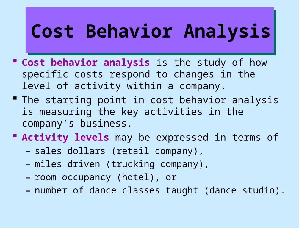
Cost Behavior Analysis

Cost behavior analysis is the study of how specific costs respond to changes in the level of activity within a company.

The starting point in cost behavior analysis is measuring the key activities in the company’s business.

Activity levels may be expressed in terms of

– sales dollars (retail company),

– miles driven (trucking company),

– room occupancy (hotel), or

– number of dance classes taught (dance studio).

Cost Behavior Analysis

For an activity level to be useful in cost behavior analysis, there should be correlation between changes in the level or volume of activity and changes in the costs.

The activity level selected is referred to as the activity (or volume) index.

The activity index identifies the activity that causes changes in the behavior of costs.

Distinguish between variable and fixed costs.

Study Objective 1

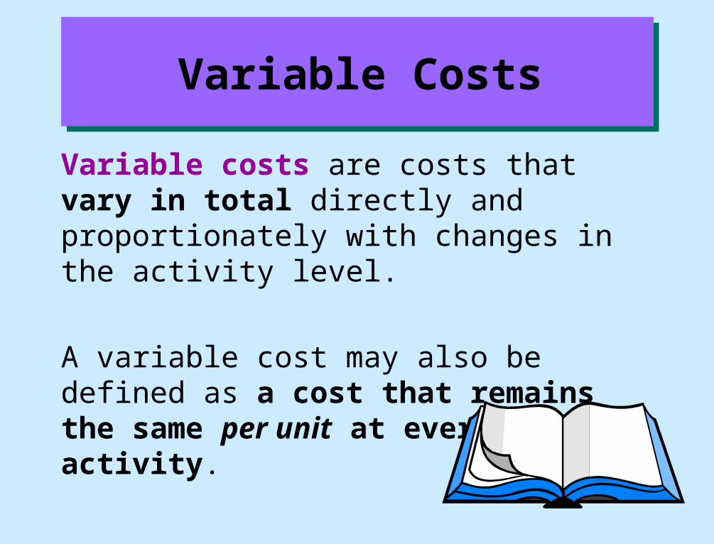
Variable Costs

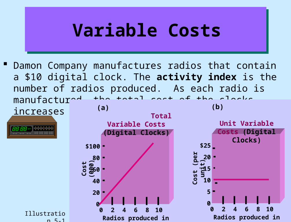
Variable costs are costs that vary in total directly and proportionately with changes in the activity level.

A variable cost may also be defined as a cost that remains the same per unit at every level of activity.

Variable Costs

Damon Company manufactures radios that contain a $10 digital clock. The activity index is the number of radios produced. As each radio is manufactured, the total cost of the clocks increases by $10.

$100

80

60

40

20

0

Co

st (

000)

0 2 4 6 8 10Radios produced in (000)

(a) Total Variable Costs

(Digital Clocks)

0

5

$25

20

15

10

Co

st (

per

un

it)

0 2 4 6 8 10Radios produced in (000)

(b) Unit Variable Costs

(Digital Clocks)

Illustration 5-1

Fixed Costs

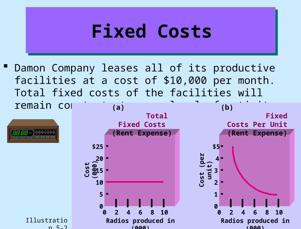
Fixed costs are costs that remain the same in total regardless of changes in the activity level.

Since fixed costs remain constant in total as activity changes, fixed costs per unit vary inversely with activity. As volume increases, unit cost declines and vice versa.

Fixed Costs

Damon Company leases all of its productive facilities at a cost of $10,000 per month. Total fixed costs of the facilities will remain constant at every level of activity.

Illustration 5-2

$25

20

15

10

5

0

Co

st (

000)

0 2 4 6 8 10Radios produced in (000)

(a) Total Fixed Costs (Rent Expense)

0

1

$5

4

3

2

Co

st (

per

un

it)

0 2 4 6 8 10Radios produced in (000)

(b) Fixed Costs Per Unit

(Rent Expense)

Explain the meaning and importance of the relevant range.

Study Objective 2

Nonlinear Behavior of Variable and Fixed Costs

In the previous two slides, the assumption was made that total variable costs and total fixed costs were linear, and straight lines were used to represent both types of costs. A straight-line relationship does not usually exist for variable costs throughout the entire range of activity.In the real world, the relationship between variable cost behavior and changes in the activity level is often curvilinear, as shown in part (a) on the right. The behavior of total fixed costs through all levels of activity is shown in part (b).

Co

st (

$)0

(b)Total Fixed Costs

Nonlinear

20 40 60 80 100Activity level (%)

Co

st (

$)

0 20 40 60 80 100Activity level (%)

(a) Total Variable Costs

Curvilinear

Illustration 5-3

Linear Behavior Within Relevant Range

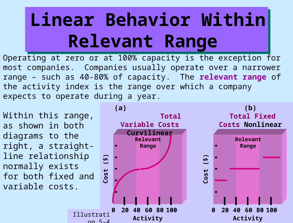
Operating at zero or at 100% capacity is the exception for most companies. Companies usually operate over a narrower range – such as 40-80% of capacity. The relevant range of the activity index is the range over which a company expects to operate during a year.

Within this range, as shown in both diagrams to the right, a straight-line relationship normally exists for both fixed and variable costs.

Illustration 5-4

Co

st (

$)0

(b) Total Fixed Costs

Nonlinear

20 40 60 80 100Activity level (%)

Relevant Range

Co

st (

$)

0 20 40 60 80 100Activity level (%)

(a) Total Variable Costs

Curvilinear

Relevant Range

Explain the concept of mixed costs.

Study Objective 3

Mixed Costs

Mixed costs contain both a variable cost element and a fixed cost element.

Sometimes called semivariable costs, mixed costs change in total but not proportionately with changes in the activity level.

Behavior of a Mixed Cost

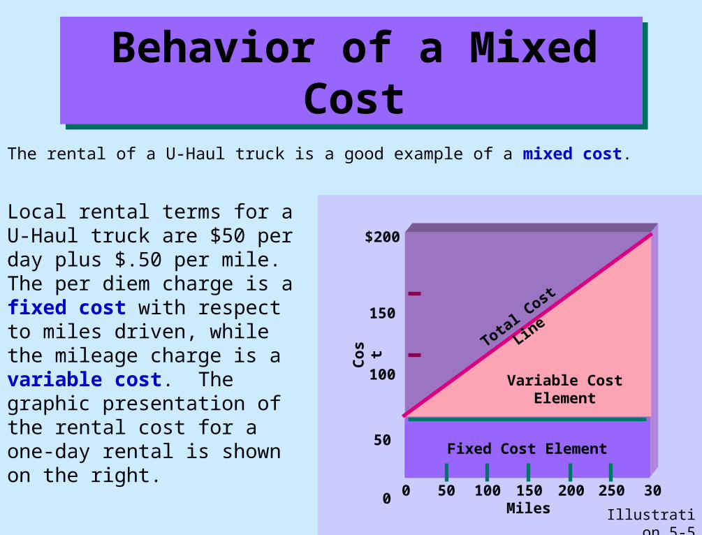
The rental of a U-Haul truck is a good example of a mixed cost.

Local rental terms for a U-Haul truck are $50 per day plus $.50 per mile. The per diem charge is a fixed cost with respect to miles driven, while the mileage charge is a variable cost. The graphic presentation of the rental cost for a one-day rental is shown on the right.

150

$200

100

50

Co

st

0

Total Cost L

ine

Variable Cost Element

Fixed Cost Element

0 50 100 150 200 250 300Miles

Illustration 5-5

Mixed Cost Classification for CVP Analysis

In CVP analysis, it is assumed that mixed costs must be classified into their fixed and variable elements.

Firms usually ascertain variable and fixed costs on an aggregate basis at the end of a time period, using the company’s past experience with the behavior of the mixed cost at various activity levels.

The high-low method is a mathematical method that uses the total costs incurred at the high and low levels of activity.

The High-Low Method

The steps in calculating fixed and variable costs under this method are as follows:

1 Determine variable cost per unit from the following formula:

2 Determine the fixed cost by subtracting the total variable cost at either the high or the low activity level from the total cost at that activity level.

Illustration 5-6

Change inTotal Costs

High minus Low Activity Level

Variable Costper Unit =

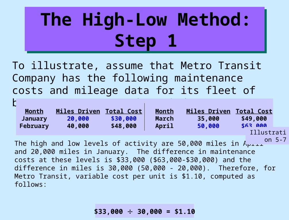
The High-Low Method:Step 1

To illustrate, assume that Metro Transit Company has the following maintenance costs and mileage data for its fleet of busses over a 4-month period:

The high and low levels of activity are 50,000 miles in April and 20,000 miles in January. The difference in maintenance costs at these levels is $33,000 ($63,000-$30,000) and the difference in miles is 30,000 (50,000 - 20,000). Therefore, for Metro Transit, variable cost per unit is $1.10, computed as follows:

$33,000 30,000 = $1.10

MonthJanuaryFebruary

Miles Driven20,00040,000

Total Cost$30,000$48,000

MonthMarchApril

Miles Driven35,00050,000

Total Cost$49,000$63,000

Illustration 5-7

The High-Low Method:Step 2

Metro Transit Company would compute the fixed portion of its maintenance costs as shown below:

Maintenance costs are therefore $8,000 per month plus $1.10 per mile. For example at 45,000 miles, estimated maintenance costs would be $49,500 variable (45,000 x $1.10), and $8,000 fixed.

Illustration 5-8

Total CostLess: Variable costs (50,000 x $1.10) (20,000 x $1.10)Total fixed costs

High $63,000

55,000

$ 8,000

Low $30,000

22,000$ 8,000

Activity Level

The High-Low Method

The high-low method generally produces a reasonable estimate for analysis.

However, it does not produce a precise measurement of the fixed and variable elements in a mixed cost because other activity levels are ignored in the computation.

!

State the five components of cost-volume-profit analysis.

Study Objective 4

Cost-Volume Profit Analysis

Cost-volume-profit (CVP) analysis is the study of the effects of changes of costs and volume on a company’s profits.

CVP analysis involves a consideration of the interrelationships among the following components:

– Volume or activity level

– Unit selling price

– Variable cost per unit

– Total fixed costs

– Sales mix

CVP Assumptions

The following assumptions underlie each CVP application: When these assumptions are not valid, the results of CVP analysis may be inaccurate.

1 The behavior of both costs and revenues is linear throughout the relevant range of the activity index.

2 All costs can be classified as either variable or fixed with reasonable accuracy.

3 Changes in activity are the only factors that affect costs.

4 All units produced are sold.

5 When more than one type of product is sold, total sales will be in a constant sales mix.

CVP Analysis

In CVP analysis applications, the term cost includes manufacturing costs plus selling and administrative expenses.

We will use Vargo Video Company as an example. Relevant data for the VCRs made by this company are as follows:

Unit selling priceUnit variable costs

Total monthly fixed costs

$500$300

$200,000

Illustration 5-10

Indicate the meaning of contribution margin and the ways it may be

expressed.

Study Objective 5

Contribution Margin

One of the key relationships in CVP analysis is contribution margin (CM). Contribution margin is the amount of revenue remaining after deducting variable costs. The CM is then available to cover fixed costs and to contribute income for the company. For example, assume that Vargo Video sells 1,000 VCRs in

one month, sales are $500,000 (1,000 x $500) and variable costs are $300,000 (1,000 x $300). Thus, contribution margin is $200,000, computed as follows:

Sales Variable CostsContribution

Margin- =

$500,000 $300,000 $200,000- =

Illustration 5-11

Unit Contribution Margin

Views differ as to the best way to express contribution margin (CM). Some favor a per unit basis.

At Vargo Video, the contribution margin per unit is $200.

Unit Selling PriceUnit Variable

CostContribution

Margin per Unit- =

$500 $300 $200- =

Illustration 5-12

CM per unit indicates that for every VCR sold, Vargo Video will have $200 to cover fixed costs and contribute to income.

Contribution Margin Ratio

Others prefer to use a contribution margin ratio.

At Vargo Video, the contribution margin ratio is 40%.

Contribution Margin per Unit

Unit Selling PriceContribution Margin Ratio =

$200 $500 40% =

Illustration 5-13

The CM ratio means that 40 cents of each sales dollar ($1 x 40%) is available to apply to fixed costs and to contribute to income.

Identify the three ways that the break-even point may be determined.

Study Objective 6

Break-Even Analysis

The second key relationship in CVP analysis is the break-even point, which is the level of activity where total revenues equals total costs, both fixed and variable.

Since no income is involved when the break-even point is the objective, the analysis is often referred to as break-even analysis.

Break-Even Analysis

The break-even point can be:

– Computed from a mathematical equation.

– Computed by using contribution margin.

– Derived from a CVP graph. The break-even point can be expressed in

either sales dollars or sales units.

Break-Even Analysis: Mathematical Equation

In its simplest form, the equation for break-even sales is:

Break-even Sales Variable Costs Fixed Costs= +

Illustration 5-14

Break-Even Analysis: Mathematical Equation for Dollars

The break-even point in dollars is found by expressing variable costs as a percentage of unit selling price.

For Vargo Video, the percentage is 60% ($300 $500). Sales must be $500,000 for Vargo Video to break even. The computation to determine sales dollars at the break-even point is:

Illustration 5-15

X = .60X + $200,000.40X = $200,000 X = $500,000

where: X = sales dollars at the break-even point .60 = variable costs as a percentage of unit selling price $200,000 = total fixed costs

Break-Even Analysis: Mathematical Equation for Units

The break-even point in units can be computed directly from the mathematical equation by using unit selling prices and unit variable costs. Vargo must sell 1,000 units to break even. The computation is:

Illustration 5-16

$500X = $300X + $200,000$200X = $200,000 X = 1,000 units

where: X = sales volume $500 = unit selling price $300 = variable cost per unit $200,000 = total fixed costs

Break-Even Analysis: Mathematical Equation Proof

The accuracy of the previous computations can be proved as follows:

Illustration 5-16

$300,000 200,000

Sales (1,000 x $500)Total costs: Variable (1,000 x $300) FixedNet Income

$500,000

500,000$ -0-

Break-Even Analysis:CM Technique for Units

Because we know that CM equals total revenues less variable costs, it follows that at the break-even point, contribution margin must equal total fixed costs.

When the CM per unit is used, the formula to compute break-even point in units is shown below:

Once again, the CM per unit for Vargo Video is $200.

Fixed CostsContribution

Margin per UnitBreak-even Point

in Units =

$200,000 $200 1,000 =

Break-Even Analysis:CM Technique for Dollars

When the CM ratio is used, the formula to compute break-even point in dollars is shown below:

Again, the CM ratio for Vargo Video is 40%.

Fixed CostsContribution Margin Ratio

Break-even Point in Dollars =

$200,000 40% $500,000 =

Break-Even Analysis:Graphic Presentation

An effective way to derive the break-even point is to prepare a break-even graph.

The graph is referred to as a cost-volume-profit (CVP) graph since it shows costs, volume, and profits.

Break-Even Analysis:Graphic Presentation

The construction of the graph, using the Vargo Video Company data, is as follows:

1 Plot the total revenue line starting at the zero activity level.

2 Plot the total fixed cost by a horizontal line.

3 Plot the total cost line starting at the fixed cost line at zero activity and increasing the amount by the variable cost at each level of activity.

4 Determine the break-even point from the intersection of the total cost line and the total revenue line.

In addition to identifying the break-even point, the CVP graph shows both the net income and net loss areas. Thus, the amount of income or loss at each level of sales can be derived from the total sales and total cost lines.

CVP Graph

In the graph to the right, sales volume is shown on the horizontal axis. This axis needs to extend to the maximum level of expected sales. Both total revenues (sales) and total costs (fixed plus variable) are recorded on the vertical axis.

Do

llars

(00

0)

Units of Sales

$900

700

600

500

400

300

200

100

1200200 400 600 800 1000 1400 1600 1800

Break-even Point

Profit Area

Sales Line

Total CostLine

Fixed CostLineLoss

Area

Illustration 5-20

Define margin of safety and give the formulas for computing it.

Study Objective 7

Margin of Safety

The margin of safety is another relationship that may be calculated in CVP analysis. Margin of safety is the difference between actual or expected sales and sales at the break-even point

This relationship measures the “breathing room” or “cushion” that management has in order to break even if actual sales fail to materialize.

Margin of Safety

The margin of safety may be expressed in dollars or as a ratio. Assuming that actual (expected) sales for Vargo Video are

$750,000, the computations are:

Actual (Expected) Sales

Break-even SalesMargin of Safety

in Dollars- =

$750,000 $500,000 $250,000- =

Margin of Safety in Dollars

Margin of Safety in Dollars

Actual (Expected) Sales

Margin of Safety Ratio =

$250,000 $750,000 33% =

Margin of Safety Ratio

Give the formulas for determining sales required to earn target net

income.

Study Objective 8

Target Net Income

Management usually sets an income objective for individual product lines. This objective, called target net income, is extremely useful to management because it indicates the sales necessary to achieve a specified level of income.

The amount of sales necessary to achieve target net income can be determined from each of the approaches used in determining break-even sales.

Target Net Income: Mathematical Equation

We know that at the break-even point no profit or loss results for the company. By adding a factor for target net income to the break-even equation, we obtain the formula shown below for determining required sales.

Required sales may be expressed in either sales dollars or sales units.

Illustration 5-23

Required Sales = Variable

Costs + Fixed Costs +

Target Net

Income

Target Net Income: Mathematical Equation

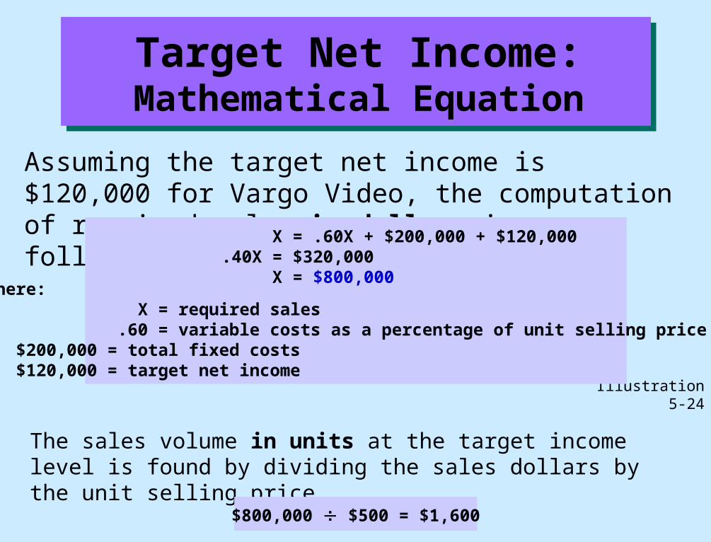
Assuming the target net income is $120,000 for Vargo Video, the computation of required sales in dollars is as follows:

Illustration 5-24

X = .60X + $200,000 + $120,000.40X = $320,000 X = $800,000

where: X = required sales .60 = variable costs as a percentage of unit selling price $200,000 = total fixed costs $120,000 = target net income

The sales volume in units at the target income level is found by dividing the sales dollars by the unit selling price.

$800,000 $500 = $1,600

Target Net Income:CM Technique

As in the case of break-even sales, the sales required to meet a target net income can be computed in either dollars or units.

The formula using the CM ratio for Video Vargo is as follows:

Required SalesFixed Costs +

Target Net Income

Contribution Margin Ratio

$320,000 40% $800,000=

=

Target Net Income:Graphic Presentation

A CVP graph can also be used to derive the sales required to meet target net income.

In the profit area of the graph, the distance between the sales line and the total cost line at any point equals net income. Required sales are found by analyzing the differences between the two lines until the desired net income is found.

CVP and Changes in the Business Environment

Business conditions change rapidly and management must respond intelligently to these changes.

CVP analysis can be used in responding to change. The original VCR sales and cost data for Vargo

Video Company are shown below.

Unit selling price $ 500Unit variable cost $ 300Total fixed costs $ 200,000Break-even sales $ 500,000 or 1,000 units

Illustration 5-26

Fixed Costs ÷ Contribution Margin per Unit = Break-even Sales

$ 200,000 ÷ $ 150 = 1,333 units (rounded)

Illustration 5-27

A competitor is offering a 10% discount on the selling price of its VCRs. Management must decide whether or not to offer a similar discount.

Question: What effect will a 10% discount on selling price have on the break-even point for VCRs?

Answer: A 10% discount on selling price reduces the selling price per unit to $450 [$500 – ($500 x 10%)]. Variable cost per unit remains unchanged at $300. Therefore, the contribution margin per unit is $150. Assuming no change in fixed costs, break-even sales are 1,333 units, calculated as follows:

CVP and Changes in the Business Environment: Case I

Fixed Costs ÷ Contribution Margin per Unit = Break-even Sales

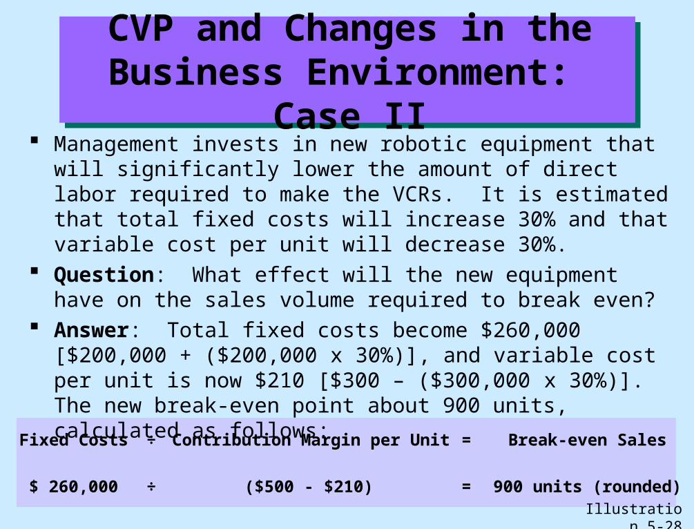
$ 260,000 ÷ ($500 - $210) = 900 units (rounded)

Illustration 5-28

Management invests in new robotic equipment that will significantly lower the amount of direct labor required to make the VCRs. It is estimated that total fixed costs will increase 30% and that variable cost per unit will decrease 30%.

Question: What effect will the new equipment have on the sales volume required to break even?

Answer: Total fixed costs become $260,000 [$200,000 + ($200,000 x 30%)], and variable cost per unit is now $210 [$300 – ($300,000 x 30%)]. The new break-even point about 900 units, calculated as follows:

CVP and Changes in the Business Environment: Case II

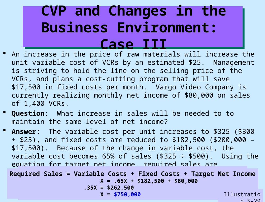
An increase in the price of raw materials will increase the unit variable cost of VCRs by an estimated $25. Management is striving to hold the line on the selling price of the VCRs, and plans a cost-cutting program that will save $17,500 in fixed costs per month. Vargo Video Company is currently realizing monthly net income of $80,000 on sales of 1,400 VCRs.

Question: What increase in sales will be needed to to maintain the same level of net income?

Answer: The variable cost per unit increases to $325 ($300 + $25), and fixed costs are reduced to $182,500 ($200,000 – $17,500). Because of the change in variable cost, the variable cost becomes 65% of sales ($325 ÷ $500). Using the equation for target net income, required sales are calculated to be $750,000, as follows:

CVP and Changes in the Business Environment: Case III

Required Sales = Variable Costs + Fixed Costs + Target Net Income X = .65X + $182,500 + $80,000 .35X = $262,500 X = $750,000

Illustration 5-29

Describe the essential features of a cost-volume-profit income statement.

Study Objective 9

CVP Income Statement

The CVP income statement classifies costs and expenses as variable or fixed and specifically reports contribution margin in the body of the statement.

The CVP income statement format is sometimes called the contribution margin format.

This format is for internal management use only.

Variable Fixed Total

Cost of goods sold $ 400,000 $ 120,000 $ 520,000

Selling expenses 60,000 40,000 100,000

Administrative expenses 20,000 40,000 60,000

$ 480,000 $ 200,000 $ 680,000

CVP Income Statement

For purposes of illustrating the CVP income statement, assume that Vargo Video Company reaches its target net income of $120,000. From an analysis of the transactions, the following information is obtained on the $680,000 of costs that were incurred in June:

Illustration 5-30

Traditional versus CVP Income Statement

The CVP income statement and the traditional income statement based on this data are shown side-by-side on the next slide.

Note that net income is the same ($120,000) in both of the statements.

The major difference is the format for the expenses. Also, the traditional statement shows gross profit,

whereas the CVP statement shows contribution margin.

Traditional versus CVP Income Statement

Traditional FormatSales $ 800,000Cost of goods sold 520,000

Gross profit 280,000Operating expenses

Selling expenses $ 100,000Administrative expenses 60,000

Total operating expenses 160,000Net income $ 120,000

CVP FormatSales $ 800,000Variable expenses

Cost of goods sold $ 400,000Selling expenses 60,000Administrative expenses 20,000

Total variable expenses 480,000Contribution margin 320,000Fixed expenses

Cost of goods sold 120,000Selling expenses 40,000Administrative expenses 40,000

Total fixed expenses 200,000Net income $ 120,000

Illustration 5-31

Appendix 5A

Variable Costing

Explain the difference between absorption costing and variable

costing.

Appendix 5AStudy Objective 10

Absorption versus Variable Costing

All manufacturing costs are charged to and absorbed by the product under full or absorption costing. This is how costs were handled in previous chapters.

Under variable costing only direct materials, direct labor, and variable manufacturing overhead costs are considered product costs. Fixed manufacturing overhead costs are recognized as period costs when incurred.

The difference between absorption costing and variable costing is graphically shown below.

Fixed Manufacturing

Overhead

Illustration 5A-1

Product Cost

Absorption Costing

Period Cost

Variable Costing

Absorption versus Variable Costing: An Illustration

As an illustration, Premium Products Corporation manufactures a polyurethane sealant called Fix-it for car windshields. Relevant data for Fix-it in January 1996, the first month of production, is as follows:

– Selling Price: $20 per unit.

– Units: Produced 30,000; sold 20,000; beginning inventory zero.

– Variable unit costs: Manufacturing $9 (direct materials $5, direct labor $3, and variable overhead $1) and selling and administrative expenses $2.

– Fixed costs: Manufacturing overhead $120,000, and selling and administrative expenses $15,000.

The per unit production cost under each costing approach is:

Absorption versus Variable Costing: Unit Production Cost

Absorption VariableType of Cost Costing Costing

Direct materials $ 5 $ 5Direct labor 3 3Variable manufacturing overhead 1 1Fixed manufacturing overhead ($120,000 ÷ 30,000 units produced) 4 0Total unit cost $ 13 $ 9

Illustration 5A-2

The difference in total unit cost of $4 ($13 - $9) occurs because fixed manufacturing costs are a product cost under absorption costing and a period cost under variable costing.

The income statements under the two costing approaches are shown on the next two slides.

Income from operations under absorption costing is $40,000 higher than under variable costing ($85,000 – $45,000). There is a $40,000 difference in the ending inventories ($130,000 under absorption costing and $90,000 under variable costing).

Under absorption costing, $40,000 of the fixed overhead costs have been deferred to a future period as a product cost.

Absorption versus Variable Costing: Effects on Income

Sales (20,000 units X $20) $ 400,000Cost of goods sold Inventory, January 1 $ –0– Cost of goods manufactured (30,000 units X $13) 390,000 Cost of goods available for sale 390,000 Inventory, January 31 (10,000 units X $13) 130,000 Cost of goods sold (20,000 units X $13) 260,000Gross profit 140,000Selling and administrative expenses (Variable 20,000 units X $2 + fixed $15,000) 55,000Income from operations $ 85,000

Absorption Costing Income Statement

Illustration 5A-3

Sales (20,000 units X $20) $ 400,000Variable expenses Variable cost of goods sold Inventory, January 1 –0–

Variable manufacturing costs (30,000 units X $9) 270,000 Cost of goods available for sale 270,000 Inventory, January 31 (10,000 units X $9) 90,000

Variable cost of goods sold 180,000 Variable selling and administrative expenses

(20,000 units X $2) 40,000 Total variable expenses 220,000Contribution margin 180,000Fixed expenses Manufacturing overhead 120,000 Selling and administrative expenses 15,000

Total fixed expenses 135,000Income from operations $ 45,000

Variable Costing Income Statement

Illustration5A-4

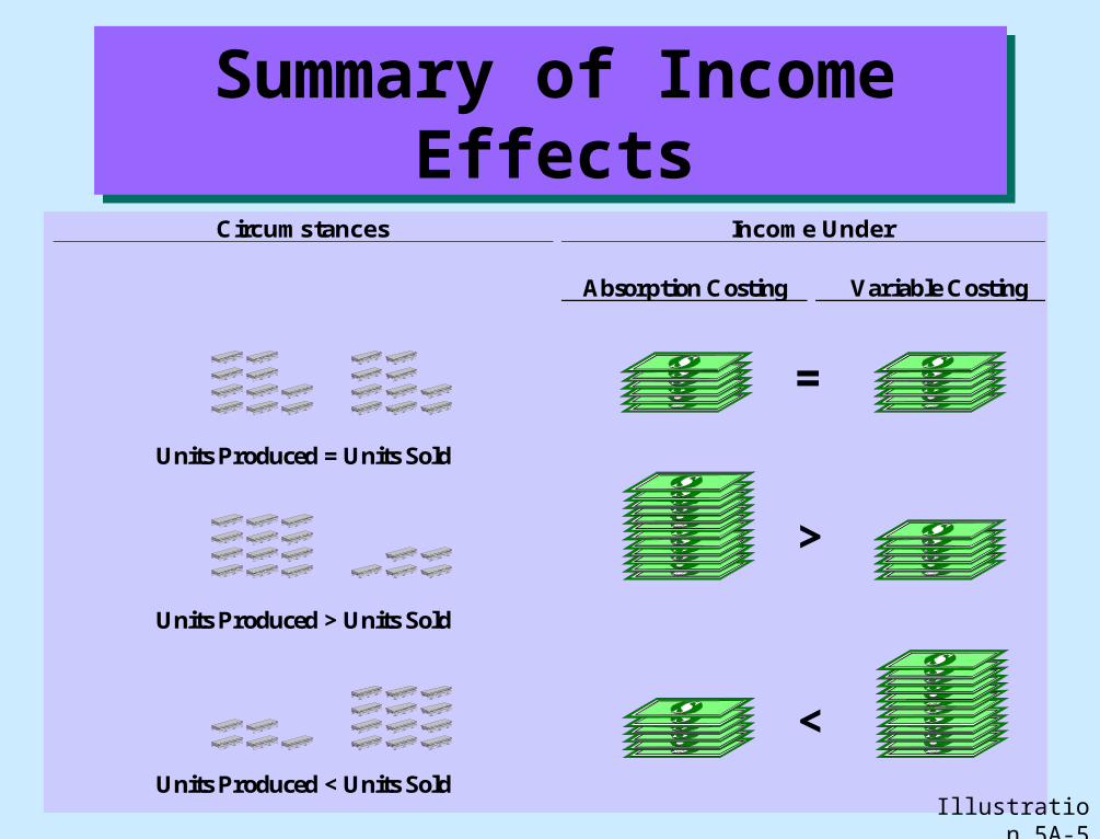
Summary of Income Effects

Circumstances Income Under

Absorption Costing Variable Costing

Units Produced = Units Sold

Units Produced > Units Sold

Units Produced < Units Sold

=

>

<

Illustration 5A-5

Rationale for Variable Costing

The rationale for variable costing focuses on the purpose of fixed manufacturing costs, which is to have productive facilities available for use.

Defenders of absorption costing justify the assignment of fixed manufacturing overhead costs to inventory on the basis that these costs are as much a cost of getting a product ready for sale as direct materials or direct labor.

The use of variable costing in product costing is acceptable only for internal use by management.

Copyright © 1999 John Wiley & Sons, Inc. All rights reserved. Reproduction or translation of this work beyond that named in Section 117 of the 1976 United States Copyright Act without the express written permission of the copyright owner is unlawful. Request for further information should be addressed to the Permissions Department, John Wiley & Sons, Inc. The purchaser may make back-up copies for his/her own use only and not for distribution or resale. The Publisher assumes no responsibility for errors, omissions, or damages, caused by the use of these programs or from the use of the information contained herein.

Copyright © 1999 John Wiley & Sons, Inc. All rights reserved. Reproduction or translation of this work beyond that named in Section 117 of the 1976 United States Copyright Act without the express written permission of the copyright owner is unlawful. Request for further information should be addressed to the Permissions Department, John Wiley & Sons, Inc. The purchaser may make back-up copies for his/her own use only and not for distribution or resale. The Publisher assumes no responsibility for errors, omissions, or damages, caused by the use of these programs or from the use of the information contained herein.

Copyright

Chapter 5Cost-Volume-Profit Relationships