Johansen Et Al-2000-The Econometrics Journal

Econometrics Journal (2000), volume 3, pp. 216–249.

Cointegration analysis in the presence of structural breaks inthe deterministic trend

SØREN JOHANSEN†, ROCCO MOSCONI‡, BENT NIELSEN§

†Economics Department, European University Institute, Via Roccettini 9,50016 San Domenico di Fiesole, Italy

E-mail: [email protected]://www.iue.it/Personal/Johansen

‡Dipartimento di Economia e Produzione, Politecnico di Milano, Piazza L. da Vinci 32,20133 Milano, Italy

E-mail: [email protected]://www.ecopro.polimi.it/home/Rocco.Mosconi

§Department of Economics, University of Oxford & Nuffield College,Oxford OX1 1NF, UK

E-mail: [email protected]://www.nuff.ox.ac.uk/users/nielsen

Summary When analysing macroeconomic data it is often of relevance to allow for struc-tural breaks in the statistical analysis. In particular, cointegration analysis in the presence ofstructural breaks could be of interest. We propose a cointegration model with piecewise lineartrend and known break points. Within this model it is possible to test cointegration rank,restrictions on the cointegrating vector as well as restrictions on the slopes of the broken lineartrend.

Keywords: Break points, Cointegration, Common trend, Deterministic trend, Piecewiselinear trend, Stochastic trend, Structural breaks, Vector autoregressive model.

1. Introduction

In the analysis of economic time series it is often necessary to allow breaks in the deterministiccomponents. When allowing for breaks the timing is important, this could either be known inadvance or an algorithm searching for breaks could be applied. While both issues are discussedin the literature and mainly in a univariate setting, this paper focuses on cointegration analysis ina multivariate setting in the presence of breaks at known points in time. The suggested approachis a slight generalization of the likelihood-based cointegration analysis in vector autoregressivemodels suggested by Johansen (1988, 1996). There are only a few conceptual differences andthe major issue for the practitioner is that new asymptotic tables are needed. This paper concernsonly asymptotic analysis. Finite sample properties of the rank test and tests for restrictions on thecointegrating vector have been discussed by Johansen (2000a,b,c) in the situation of no breaksusing an analytic correction factor to the likelihood ratio tests.

c© Royal Economic Society 2000. Published by Blackwell Publishers Ltd, 108 Cowley Road, Oxford OX4 1JF, UK and 350 Main Street,Malden, MA, 02148, USA.

n

Highlight

Cointegration analysis 217

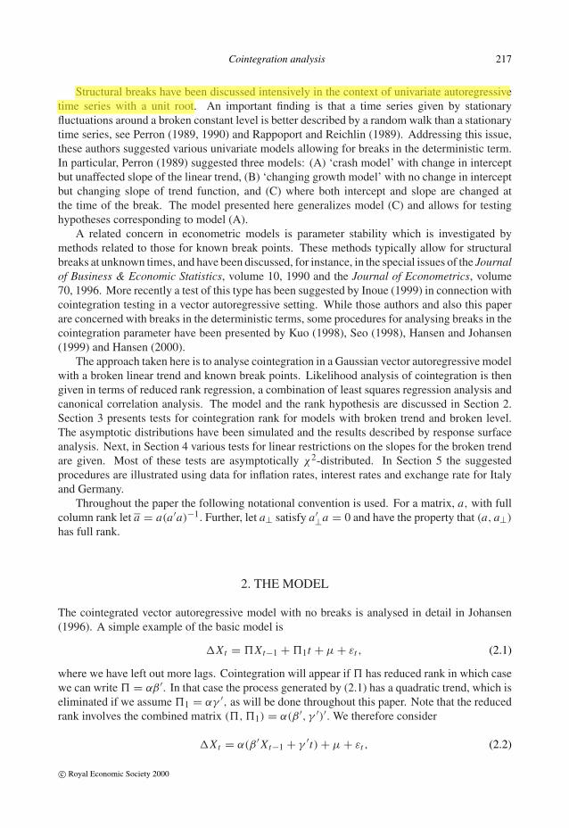
Structural breaks have been discussed intensively in the context of univariate autoregressivetime series with a unit root. An important finding is that a time series given by stationaryfluctuations around a broken constant level is better described by a random walk than a stationarytime series, see Perron (1989, 1990) and Rappoport and Reichlin (1989). Addressing this issue,these authors suggested various univariate models allowing for breaks in the deterministic term.In particular, Perron (1989) suggested three models: (A) ‘crash model’ with change in interceptbut unaffected slope of the linear trend, (B) ‘changing growth model’ with no change in interceptbut changing slope of trend function, and (C) where both intercept and slope are changed atthe time of the break. The model presented here generalizes model (C) and allows for testinghypotheses corresponding to model (A).

A related concern in econometric models is parameter stability which is investigated bymethods related to those for known break points. These methods typically allow for structuralbreaks at unknown times, and have been discussed, for instance, in the special issues of the Journalof Business & Economic Statistics, volume 10, 1990 and the Journal of Econometrics, volume70, 1996. More recently a test of this type has been suggested by Inoue (1999) in connection withcointegration testing in a vector autoregressive setting. While those authors and also this paperare concerned with breaks in the deterministic terms, some procedures for analysing breaks in thecointegration parameter have been presented by Kuo (1998), Seo (1998), Hansen and Johansen(1999) and Hansen (2000).

The approach taken here is to analyse cointegration in a Gaussian vector autoregressive modelwith a broken linear trend and known break points. Likelihood analysis of cointegration is thengiven in terms of reduced rank regression, a combination of least squares regression analysis andcanonical correlation analysis. The model and the rank hypothesis are discussed in Section 2.Section 3 presents tests for cointegration rank for models with broken trend and broken level.The asymptotic distributions have been simulated and the results described by response surfaceanalysis. Next, in Section 4 various tests for linear restrictions on the slopes for the broken trendare given. Most of these tests are asymptotically χ2-distributed. In Section 5 the suggestedprocedures are illustrated using data for inflation rates, interest rates and exchange rate for Italyand Germany.

Throughout the paper the following notational convention is used. For a matrix, a, with fullcolumn rank let a = a(a′a)−1. Further, let a⊥ satisfy a′⊥a = 0 and have the property that (a, a⊥)

has full rank.

2. The Model

The cointegrated vector autoregressive model with no breaks is analysed in detail in Johansen(1996). A simple example of the basic model is

�Xt = �Xt−1 + �1t + µ + εt , (2.1)

where we have left out more lags. Cointegration will appear if � has reduced rank in which casewe can write � = αβ ′. In that case the process generated by (2.1) has a quadratic trend, which iseliminated if we assume �1 = αγ ′, as will be done throughout this paper. Note that the reducedrank involves the combined matrix (�, �1) = α(β ′, γ ′)′. We therefore consider

�Xt = α(β ′ Xt−1 + γ ′t) + µ + εt , (2.2)

c© Royal Economic Society 2000

n

Highlight

218 S. Johansen et al.

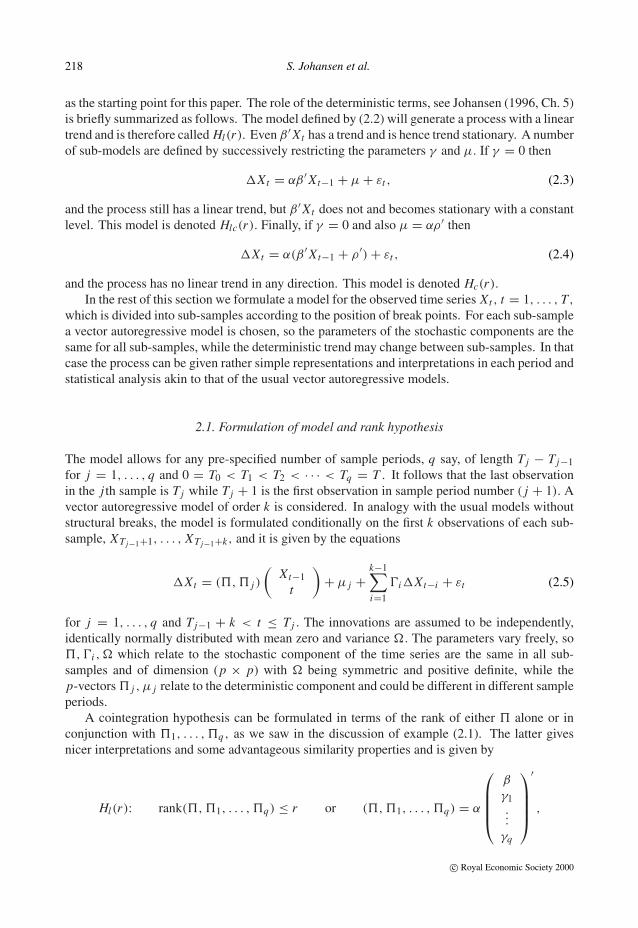
as the starting point for this paper. The role of the deterministic terms, see Johansen (1996, Ch. 5)is briefly summarized as follows. The model defined by (2.2) will generate a process with a lineartrend and is therefore called Hl(r). Even β ′ Xt has a trend and is hence trend stationary. A numberof sub-models are defined by successively restricting the parameters γ and µ. If γ = 0 then

�Xt = αβ ′ Xt−1 + µ + εt , (2.3)

and the process still has a linear trend, but β ′ Xt does not and becomes stationary with a constantlevel. This model is denoted Hlc(r). Finally, if γ = 0 and also µ = αρ′ then

�Xt = α(β ′ Xt−1 + ρ′) + εt , (2.4)

and the process has no linear trend in any direction. This model is denoted Hc(r).

In the rest of this section we formulate a model for the observed time series Xt , t = 1, . . . , T,

which is divided into sub-samples according to the position of break points. For each sub-samplea vector autoregressive model is chosen, so the parameters of the stochastic components are thesame for all sub-samples, while the deterministic trend may change between sub-samples. In thatcase the process can be given rather simple representations and interpretations in each period andstatistical analysis akin to that of the usual vector autoregressive models.

2.1. Formulation of model and rank hypothesis

The model allows for any pre-specified number of sample periods, q say, of length Tj − Tj−1for j = 1, . . . , q and 0 = T0 < T1 < T2 < · · · < Tq = T . It follows that the last observationin the j th sample is Tj while Tj + 1 is the first observation in sample period number ( j + 1). Avector autoregressive model of order k is considered. In analogy with the usual models withoutstructural breaks, the model is formulated conditionally on the first k observations of each sub-sample, XTj−1+1, . . . , XTj−1+k, and it is given by the equations

�Xt = (�, � j )

(Xt−1

t

)+ µ j +

k−1∑i=1

�i�Xt−i + εt (2.5)

for j = 1, . . . , q and Tj−1 + k < t ≤ Tj . The innovations are assumed to be independently,identically normally distributed with mean zero and variance �. The parameters vary freely, so�, �i , � which relate to the stochastic component of the time series are the same in all sub-samples and of dimension (p × p) with � being symmetric and positive definite, while thep-vectors � j , µ j relate to the deterministic component and could be different in different sampleperiods.

A cointegration hypothesis can be formulated in terms of the rank of either � alone or inconjunction with �1, . . . , �q , as we saw in the discussion of example (2.1). The latter givesnicer interpretations and some advantageous similarity properties and is given by

Hl(r): rank(�, �1, . . . , �q) ≤ r or (�, �1, . . . , �q) = α

β

γ1...

γq

′

,



where the parameters vary freely so α, β are of dimension (p × r ) and γ j is of dimension (1 × r ).The notation Hl indicates that in each sub-sample the deterministic component is linear both fornon-stationary and cointegrating relations. This feature will become evident from the Grangerrepresentation below. A related hypothesis arises in the case of no linear trend but a brokenconstant level as in example (2.4),

Hc(r): rank(�, µ1, . . . , µq) ≤ r and �1, . . . , �q = 0.

As an alternative to the models Hl and Hc a rank hypothesis could be formulated for � alone asin example (2.3),

Hlc(r): rank � ≤ r and �1, . . . , �q = 0.

The hypotheses are nested as Hc(r) ⊂ Hlc(r) ⊂ Hl(r).

For the purpose of determining the cointegration rank the hypothesis Hlc is less attractive thanHc, Hl for two reasons. First, as indicated by the sub-index, the hypothesis Hlc implies that thenon-stationary relations have a broken linear trend while the cointegrating relations have brokenconstant levels. Thus under the hypothesis Hlc the deterministic trend of a component dependson the cointegrating properties, whereas in testing Hl the deterministic behaviour of the processis the same regardless of the cointegrating properties, namely a linear trend in all directions.Secondly, in Section 3.3 it will be demonstrated that the asymptotic analysis is heavily burdenedwith nuisance parameters. These issues are discussed in further detail by Nielsen and Rahbek(2000).

2.2. Another formulation

The above description involves writing q model equations of type (2.5). In order to write theseas one equation which is more conformable with standard econometric computer packages somedummy variables are introduced. Let

D j,t ={

1 for t = Tj−1,

0 otherwise,for j = 2, . . . , q; t = . . . , −1, 0, 1, . . . ,

so D j,t−i is an indicator function for the i th observation in the j th period; that is, D j,t−i = 1 ift = Tj−1 + i . Further,

E j,t =Tj −Tj−1∑i=k+1

D j,t−i ={

1 for Tj−1 + k + 1 ≤ t ≤ Tj ,

0 otherwise,

is the effective sample of the j th period. It is convenient to gather the sample dummies and thedrift parameters for the different sample periods

Et = (E1,t , . . . , Eq,t )′, µ = (µ1, . . . , µq), γ = (γ ′

1, . . . , γ′q)′,

of dimensions (q × 1), (p × q), (q × r), respectively. The model equation becomes

�Xt = α

(β

γ

)′ ( Xt−1t Et

)+ µEt +

k−1∑i=1

�i�Xt−i +k∑

i=1

q∑j=2

κ j,i D j,t−i + εt , (2.6)



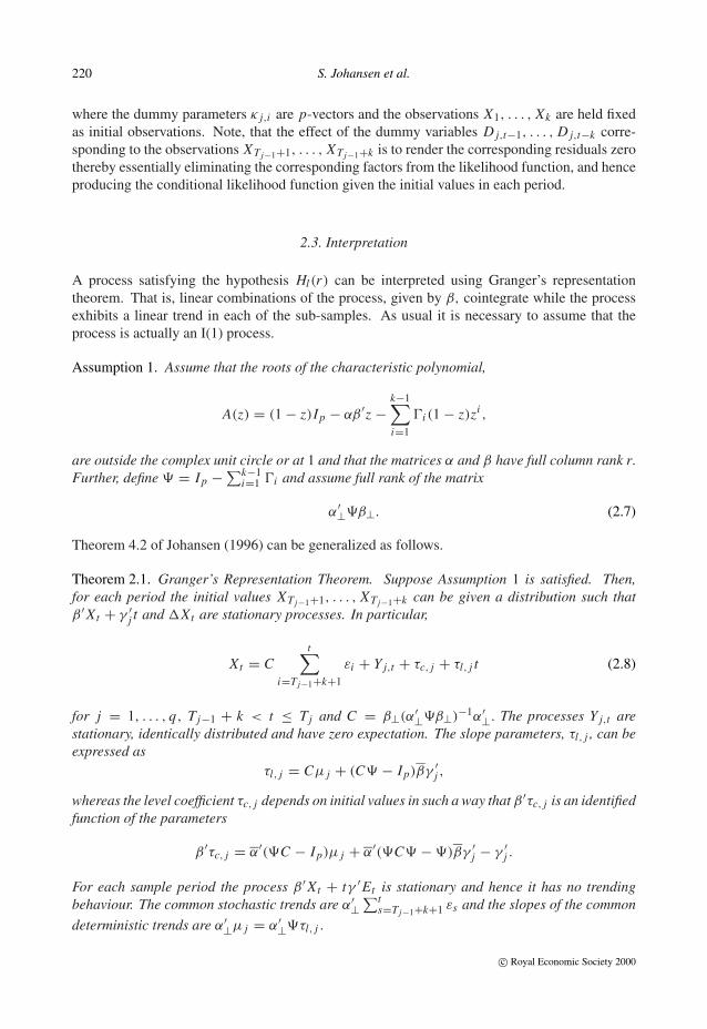
where the dummy parameters κ j,i are p-vectors and the observations X1, . . . , Xk are held fixedas initial observations. Note, that the effect of the dummy variables D j,t−1, . . . , D j,t−k corre-sponding to the observations XTj−1+1, . . . , XTj−1+k is to render the corresponding residuals zerothereby essentially eliminating the corresponding factors from the likelihood function, and henceproducing the conditional likelihood function given the initial values in each period.

2.3. Interpretation

A process satisfying the hypothesis Hl(r) can be interpreted using Granger’s representationtheorem. That is, linear combinations of the process, given by β, cointegrate while the processexhibits a linear trend in each of the sub-samples. As usual it is necessary to assume that theprocess is actually an I(1) process.

Assumption 1. Assume that the roots of the characteristic polynomial,

A(z) = (1 − z)Ip − αβ ′z −k−1∑i=1

�i (1 − z)zi ,

are outside the complex unit circle or at 1 and that the matrices α and β have full column rank r.Further, define � = Ip − ∑k−1

i=1 �i and assume full rank of the matrix

α′⊥�β⊥. (2.7)

Theorem 4.2 of Johansen (1996) can be generalized as follows.

Theorem 2.1. Granger’s Representation Theorem. Suppose Assumption 1 is satisfied. Then,for each period the initial values XTj−1+1, . . . , XTj−1+k can be given a distribution such thatβ ′ Xt + γ ′

j t and �Xt are stationary processes. In particular,

Xt = Ct∑

i=Tj−1+k+1

εi + Y j,t + τc, j + τl, j t (2.8)

for j = 1, . . . , q, Tj−1 + k < t ≤ Tj and C = β⊥(α′⊥�β⊥)−1α′⊥. The processes Y j,t arestationary, identically distributed and have zero expectation. The slope parameters, τl, j , can beexpressed as

τl, j = Cµ j + (C� − Ip)βγ ′j ,

whereas the level coefficient τc, j depends on initial values in such a way that β ′τc, j is an identifiedfunction of the parameters

β ′τc, j = α′(�C − Ip)µ j + α′(�C� − �)βγ ′j − γ ′

j .

For each sample period the process β ′ Xt + tγ ′Et is stationary and hence it has no trendingbehaviour. The common stochastic trends are α′⊥

∑ts=Tj−1+k+1 εs and the slopes of the common

deterministic trends are α′⊥µ j = α′⊥�τl, j .



In some situations it is convenient to have linear combinations of the data representing thenon-stationary trends. Examples are β ′⊥ Xt and α′⊥� Xt both of which are combinations that donot cointegrate.

The representation shows that in each sub-sample all linear combinations of the process areallowed to have a linear trend, which generalizes model (C) suggested by Perron (1989). Testsfor linear restrictions on the slope parameter τl = Cµ + (C� − Ip)βγ ′ are discussed in Section4. The Granger representation shows that the slope for the cointegrating vector, β ′τl = −γ ′, hasto be treated separately from the slope of the common deterministic trend, α′⊥�τl = α′⊥µ.

An example is the two-period model, q = 2, with common slopes, τl,1 = τl,2, correspondingto Perron’s model (A). In general these hypotheses are of the form

Hγ

l (r) : β ′τl G⊥ = −γ ′G⊥ = 0 or γ = Gϕ (2.9)

for the cointegrating relation and

Hµl (r) : α′⊥�τl M⊥ = α′⊥µM⊥ = 0

for the common deterministic trends. Here G and M are known matrices of dimension (q × g)

and (q × m), respectively, with g, m < q and full column rank. In particular, Perron’s model (A)is given by G = M = (1, 1)′, which means that γ1 = γ2 and α′⊥µ1 = α′⊥µ2.

A more subtle question is how the transition happens from one sample period to the next.The suggested conditioning on k initial values in each period allows for great flexibility and thesetransition periods can be extended if necessary. An alternative approach would be to use a specifictransition function of some kind. Suppose it is of interest to model an instantaneous break in thelevel. As a simple example of such a problem, with one lag, consider an unobserved componentsformulation

Xt = τc,11(t≤T1) + τc,21(t>T1) + Zt ,

�Zt = αβ ′Zt−1 + εt ,

such that for 2 ≤ t ≤ T,

�Xt = αβ ′{Xt−1 − τc,11(t−1≤T1) − τc,21(t−1>T1)} + τc,1�1(t≤T1) + τc,2�1(t>T1) + εt .

Using the definitions of D j,t and E j,t , in particular that D2,t = 1(t=T1), E1,t = 1(t≤T1) andE2,t = 1(t≥T1+2), it follows that

�Xt = αβ ′(Xt−1 − τc,1 E1,t − τc,2 E2,t ) + {τc,2 − (Ip + αβ ′)τc,1}D2,t−1 + εt .

Comparing with equation (2.6) or rather (3.6) it is found to be of the form

�Xt = α

(β

γ

)′ ( Xt−1Et

)+ κ2,1 D2,t−1 + εt

with γ ′j = −β ′τc, j , for j = 1, 2, and κ2,1 = τc,2 − (Ip + αβ ′)τc,1 satisfying the restriction

β ′κ2,1 = (Ir + β ′α)γ ′1 − γ ′

2.

This restriction on κ2,1 is related to only one observation and is therefore difficult to test. Formodels of higher order the conditions for instantaneous breaks would similarly involve all tran-sition parameters κ j,i . This issue is discussed in further detail for the univariate case by Perron(1990).



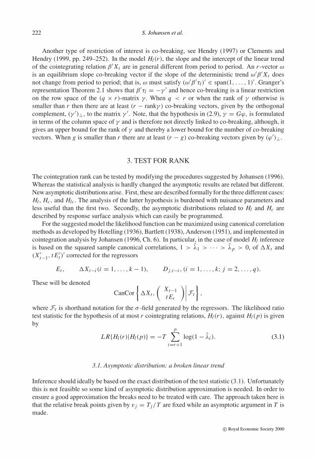
Another type of restriction of interest is co-breaking, see Hendry (1997) or Clements andHendry (1999, pp. 249–252). In the model Hl(r), the slope and the intercept of the linear trendof the cointegrating relation β ′ Xt are in general different from period to period. An r -vector ω

is an equilibrium slope co-breaking vector if the slope of the deterministic trend ω′β ′ Xt doesnot change from period to period; that is, ω must satisfy (ω′β ′τl)

′ ∈ span(1, . . . , 1)′. Granger’srepresentation Theorem 2.1 shows that β ′τl = −γ ′ and hence co-breaking is a linear restrictionon the row space of the (q × r)-matrix γ. When q < r or when the rank of γ otherwise issmaller than r then there are at least (r − rankγ ) co-breaking vectors, given by the orthogonalcomplement, (γ ′)⊥, to the matrix γ ′. Note, that the hypothesis in (2.9), γ = Gϕ, is formulatedin terms of the column space of γ and is therefore not directly linked to co-breaking, although, itgives an upper bound for the rank of γ and thereby a lower bound for the number of co-breakingvectors. When g is smaller than r there are at least (r − g) co-breaking vectors given by (ϕ′)⊥.

3. Test for Rank

The cointegration rank can be tested by modifying the procedures suggested by Johansen (1996).Whereas the statistical analysis is hardly changed the asymptotic results are related but different.New asymptotic distributions arise. First, these are described formally for the three different cases:Hl , Hc, and Hlc. The analysis of the latter hypothesis is burdened with nuisance parameters andless useful than the first two. Secondly, the asymptotic distributions related to Hl and Hc aredescribed by response surface analysis which can easily be programmed.

For the suggested model the likelihood function can be maximized using canonical correlationmethods as developed by Hotelling (1936), Bartlett (1938), Anderson (1951), and implemented incointegration analysis by Johansen (1996, Ch. 6). In particular, in the case of model Hl inferenceis based on the squared sample canonical correlations, 1 > λ1 > · · · > λp > 0, of �Xt and(X ′

t−1, t E ′t )

′ corrected for the regressors

Et , �Xt−i (i = 1, . . . , k − 1), D j,t−i , (i = 1, . . . , k; j = 2, . . . , q).

These will be denoted

CanCor

{�Xt ,

(Xt−1t Et

)∣∣∣∣Ft

},

where Ft is shorthand notation for the σ -field generated by the regressors. The likelihood ratiotest statistic for the hypothesis of at most r cointegrating relations, Hl(r), against Hl(p) is givenby

L R{Hl(r)|Hl(p)} = −Tp∑

i=r+1

log(1 − λi ). (3.1)

3.1. Asymptotic distribution: a broken linear trend

Inference should ideally be based on the exact distribution of the test statistic (3.1). Unfortunatelythis is not feasible so some kind of asymptotic distribution approximation is needed. In order toensure a good approximation the breaks need to be treated with care. The approach taken here isthat the relative break points given by v j = Tj/T are fixed while an asymptotic argument in T ismade.



For the asymptotic results the following notation is convenient. The relative break pointsv j = Tj/T satisfy 0 = v0 < v1 < · · · < vq = 1. Let �v j = v j − v j−1 and define a q-dimensional vector of indicator functions for the sample periods, eu = {. . . , 1(v j−1<u≤v j ), . . .}′.This function is the limit of E[T u] as T increases. For any two vector valued continuous functionsfu and gu on [0,1] we use the notation

( fu |gu) = fu −∫ 1

0fs g′

sds

(∫ 1

0gs g′

sds

)−1

gu,

for the residual of f after correcting for g.

Theorem 3.1. Suppose Hl(r) and Assumption 1 are satisfied. Then the asymptotic distribution ofthe likelihood ratio test statistic for Hl(r) against Hl(p) is given by

tr

{∫ 1

0dWu F ′

u

(∫ 1

0Fu F ′

udu

)−1 ∫ 1

0FudW ′

u

}(3.2)

as T → ∞ and for fixed relative break points, v j . Here W is a standard Brownian motion ofdimension (p − r) and F is a (p − r + q)-dimensional process,

Fu =(

Wu

ueu

∣∣∣∣ eu

). (3.3)

The asymptotic distribution has been simulated and the results analysed by a response surfaceanalysis presented in Section 3.4.

For analytic reasoning and for computer simulations it is convenient to rewrite the represen-tation of the distribution given by (3.2). This is based on two ideas. First, the distribution isinvariant with respect to linear transformations of the vector process F. Thus if the first (p − r)

components are regressed on the last q components giving F0,u = (Wu |ueu, eu), the transformedversion of the matrix (

∫ 10 Fu F ′

udu)−1 is block diagonal. It follows that expression (3.2) can berewritten as the sum of two terms which do not involve the levels of the Brownian motion, see(3.4) below. We find

tr

{∫ 1

0dWu F ′

0,u

(∫ 1

0F0,u F ′

0,udu

)−1 ∫ 1

0F0,udW ′

u

}

+tr

[∫ 1

0dWu(ueu |eu)′

{∫ 1

0(ueu |eu)(ueu |eu)′du

}−1 ∫ 1

0(ueu |eu)dW ′

u

].

The second term is χ2{q(p − r)}-distributed since

∫ 1

0(ueu |eu)dW ′

uD= Nq×(p−r)

{0,

∫ 1

0(ueu |eu)(ueu |eu)′du ⊗ Ip−r

}.

Secondly, when regressing a Brownian motion on the level in each of the two or more sub-samples,the sub-sample Brownian motions will be independent. These considerations lead to a secondrepresentation of the asymptotic distribution (3.2).



Theorem 3.2. Let W (1), . . . , W (q) be independent (p − r)-dimensional standard Brownian mo-tions and define

J j ={∫ 1

0(u|1)2du

}−1/2 ∫ 1

0(u|1){dW ( j)

u }′,

K j =∫ 1

0{W ( j)

u |1, u}{dW ( j)u }′,

L j =∫ 1

0{W ( j)

u |1, u}{W ( j)u |1, u}′du.

Then the limiting variable (3.2) can be expressed as

tr

(q∑

j=1

K j�v j

)′ { q∑j=1

L j (�v j )2

}−1 (q∑

j=1

K j�v j

) +

(q∑

j=1

J ′j J j

). (3.4)

From representation (3.4) of the limit distribution it is seen that the asymptotic distributiononly depends on the relative length of the sample periods, not on their ordering. For instance, inthe case of one break point, the asymptotic distribution is the same if T1 = T/3 as if T1 = 2T/3.

Moreover, the first term in (3.4) is the trace of a (p − r)-dimensional square matrix while thesecond term is the sum of inner products of (p −r)-dimensional vectors. This reflects the degreesof freedom arising from the matrix � and the vectors � j , respectively.

This representation also shows another feature of the limit distribution. In the case of q + 1sample periods let DFq+1(v1, . . . , vq+1) denote the asymptotic distribution. When the lengthsof one of the sample periods, �v j , tends to zero it follows that the contributions K j , L j vanishin the first term of (3.4). In the second term we can isolate J ′

j J j and find

lim�v j →0

DFq+1(v1, . . . , vq+1) = DFq(v1, . . . , v j−1, v j+1, . . . , vq+1) + J ′j J j , (3.5)

where DFq and J ′j J j are independent and J ′

j J j is χ2(p − r)-distributed. The additional χ2

term arises because the dimension of the vector (X ′t−1, t E ′

t ) is preserved although one of therelative sample lengths vanishes, and hence the dimension of the restrictions imposed by the rankhypothesis is unaltered. If the dummies with the vanishing sample length are taken out of thestatistical analysis the additional χ2-distributed element disappears.

The asymptotic distribution given above does not depend on the parameters for the determin-istic component. The test is therefore asymptotically similar with respect to these parametersprovided that Assumption 1 is satisfied, see also Nielsen and Rahbek (2000).

In order to estimate the rank a sequential testing procedure is necessary. One suggestion is totest the hypotheses

Hl(0), Hl(1), . . . , Hl(p − 1)

sequentially against the unrestricted model Hl(p). If Hl(r) is the first hypothesis to be acceptedthen the cointegrating rank is estimated by r. For consistency properties of this procedure seeJohansen (1996, Section 12.1).



3.2. A broken constant level

In some applications the level of the data may change from time to time but the data do not exhibita linear trend. Then the model is given by

�Xt = (�, µ)

(Xt−1Et

)+

k−1∑i=1

�i�Xt−i +k∑

i=1

q∑j=2

κ j,i D j,t−i + εt . (3.6)

The hypothesis of reduced cointegration rank is given by Hc(r): rank (�, µ) ≤ r, or equivalentlythat (�, µ) can be written as α(β ′, γ ′), while the likelihood ratio test statistic for Hc(r) againsta general alternative, Hc(p), is of form (3.1). The result of Theorem 3.1 applies with F replacedby a (p − r + q)-dimensional process with components

Fu =(

Wu

eu

). (3.7)

3.3. Models with unrestricted parameters for the broken trend

The hypothesis Hc(r) in model (3.6) imposes rank restrictions on the first-order autoregressiveparameter as well as the parameter for the broken deterministic trend. In some situations it mayseem reasonable to analyse a rank hypothesis which only involves the autoregressive parameterfor levels

Hlc(r) : rank � ≤ r or � = αβ ′,

while µ is left unrestricted. This hypothesis is analysed by correcting �Xt and Xt−1 for theremaining components in the model and subsequently performing a canonical correlation analysisof the residuals. The likelihood ratio test statistic for Hlc(r) against Hlc(p) = Hc(p) is of form(3.1). Its asymptotic distribution is given as follows.

Theorem 3.3. Suppose Hlc(r) and Assumption 1 are satisfied. Let W be a (p − r)-dimensionalstandard Brownian motion and F the (p −r +q)-dimensional process given in Theorem 3.1. Theasymptotic distribution as T → ∞ of the likelihood ratio test statistic for Hlc(r) against Hlc(p)

depends on α′⊥µ, in particular, let n = rank (α′⊥µ) ≤ min(p − r, q).

(i) Suppose n = (p − r) ≤ q. Then the asymptotic distribution is χ2{(p − r)2}.(i i) Suppose n = q < (p − r). Then the asymptotic distribution is given by

tr

{∫ 1

0dWu F ′

u N

(N ′

∫ 1

0Fu F ′

uduN

)−1

N ′∫ 1

0FudW ′

u

}(3.8)

where N is the {(p − r + q) × (p − r)}-matrix

N ′ =(

Ip−r−q 0(p−r−q)×q 00 0 Iq

). (3.9)



(i i i) Suppose n < min(p − r, q). Then there exist matrices θ, η of rank n and dimensions{(p − r) × n}, (q × n), respectively, so α′⊥µ = θη′. The asymptotic distribution is thengiven by (3.8) where N now depends on η

N ′ =(

Ip−r−n 0(p−r−n)×n 00 0 η′

). (3.10)

The test is not as attractive as the previously considered tests. The limit distribution is acomplicated function of α′⊥µ. The test is therefore not asymptotically similar with respect to theslope parameters for the broken trend. Although the third situation in Theorem 3.3 only occurson a null subset of the parameter space, the issue ought to be addressed in the statistical analysis.Had there been no breaks in the trend the test strategy suggested by Johansen (1996, Section12.2) could be used. A generalization of that idea is not simple for two reasons. First, the limitdistribution depends continuously on the nuisance parameter. Secondly, in many applications itcould be of interest subsequently to test hypotheses corresponding to rank restrictions on α′⊥µ.Such tests are discussed in Section 4.

3.4. Critical values for rank tests

Exact analytic expressions for the asymptotic distributions are not known and the quantiles haveto be determined by simulation. The asymptotic distributions depend on a number of factors:the number of non-stationary relations, the location of break points and the trend specification.The moments of these distributions have been approximated using a large number of simulationsand a subsequent response surface analysis based on these factors. Then, the quantiles can beapproximated using the empirical observation that the shape of rank test distributions typicallyare approximated rather well by �-distributions, see Nielsen (1997) and Doornik (1998). Sincethe parameters of a �-distribution are given by the first two moments, it suffices to report adequateapproximations to the asymptotic mean and variance of the trace test distributions. The quantilescan then be determined using a numerical routine for the incomplete �-integral or a χ2-distributionwith non-integer degrees of freedom which is available in most statistical computer packages.

In the following the cases with a broken trend or a broken level are considered with up tothree sample periods, q = 3. The cases with q = 1, 2, 3 can be described jointly. Let v j = Tj/Tdenote the break points as a percentage of the full sample. For the case q = 3 there are threerelative sample lengths, v1 − 0, v2 − v1, 1 − v2. Let a and b denote the smallest and the secondsmallest of these. For the case q = 2 there are two relative sample lengths v1 − 0, 1 − v1. Let bdenote the smallest of these and let a = 0. Finally, for q = 1 let a = b = 0.

The moments of the asymptotic distributions are unknown functions of (p − r), a, b. Wehave found that such functions are very accurately approximated by

log(moment) ≈ fmoment(p − r, a, b, T ) (3.11)

=2∑

m=0

αm +

4∑i=1

βim xi +4∑

i=1

∑j� i

γi jm xi x j +4∑

i=1

∑j� i

∑k� j

δi jkm xi x j xk

dm

where x1 = (p − r), x2 = a, x3 = b, x4 = T −1, dm = (p − r)−m . This function is essentially athird-order polynomial in (p −r), a, b and T −1, where the terms in (p −r)−1 and (p −r)−2 play



0.0 0.1 0.2 0.3

0.0

0.1

0.2

0.3

0.4

0.5b

a

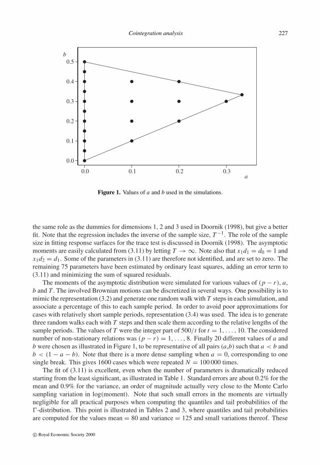
Figure 1. Values of a and b used in the simulations.

the same role as the dummies for dimensions 1, 2 and 3 used in Doornik (1998), but give a betterfit. Note that the regression includes the inverse of the sample size, T −1. The role of the samplesize in fitting response surfaces for the trace test is discussed in Doornik (1998). The asymptoticmoments are easily calculated from (3.11) by letting T → ∞. Note also that x1d1 = d0 = 1 andx1d2 = d1. Some of the parameters in (3.11) are therefore not identified, and are set to zero. Theremaining 75 parameters have been estimated by ordinary least squares, adding an error term to(3.11) and minimizing the sum of squared residuals.

The moments of the asymptotic distribution were simulated for various values of (p − r), a,b and T . The involved Brownian motions can be discretized in several ways. One possibility is tomimic the representation (3.2) and generate one random walk with T steps in each simulation, andassociate a percentage of this to each sample period. In order to avoid poor approximations forcases with relatively short sample periods, representation (3.4) was used. The idea is to generatethree random walks each with T steps and then scale them according to the relative lengths of thesample periods. The values of T were the integer part of 500/t for t = 1, . . . , 10. The considerednumber of non-stationary relations was (p − r) = 1, . . . , 8. Finally 20 different values of a andb were chosen as illustrated in Figure 1, to be representative of all pairs (a,b) such that a < b andb < (1 − a − b). Note that there is a more dense sampling when a = 0, corresponding to onesingle break. This gives 1600 cases which were repeated N = 100 000 times.

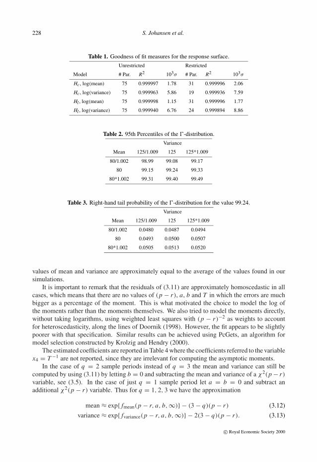
The fit of (3.11) is excellent, even when the number of parameters is dramatically reducedstarting from the least significant, as illustrated in Table 1. Standard errors are about 0.2% for themean and 0.9% for the variance, an order of magnitude actually very close to the Monte Carlosampling variation in log(moment). Note that such small errors in the moments are virtuallynegligible for all practical purposes when computing the quantiles and tail probabilities of the�-distribution. This point is illustrated in Tables 2 and 3, where quantiles and tail probabilitiesare computed for the values mean = 80 and variance = 125 and small variations thereof. These



Table 1. Goodness of fit measures for the response surface.

Unrestricted Restricted

Model # Par. R2 103σ # Par. R2 103σ

Hc , log(mean) 75 0.999997 1.78 31 0.999996 2.06

Hc , log(variance) 75 0.999963 5.86 19 0.999936 7.59

Hl , log(mean) 75 0.999998 1.15 31 0.999996 1.77

Hl , log(variance) 75 0.999940 6.76 24 0.999894 8.86

Table 2. 95th Percentiles of the �-distribution.

Variance

Mean 125/1.009 125 125*1.009

80/1.002 98.99 99.08 99.17

80 99.15 99.24 99.33

80*1.002 99.31 99.40 99.49

Table 3. Right-hand tail probability of the �-distribution for the value 99.24.

Variance

Mean 125/1.009 125 125*1.009

80/1.002 0.0480 0.0487 0.0494

80 0.0493 0.0500 0.0507

80*1.002 0.0505 0.0513 0.0520

values of mean and variance are approximately equal to the average of the values found in oursimulations.

It is important to remark that the residuals of (3.11) are approximately homoscedastic in allcases, which means that there are no values of (p − r), a, b and T in which the errors are muchbigger as a percentage of the moment. This is what motivated the choice to model the log ofthe moments rather than the moments themselves. We also tried to model the moments directly,without taking logarithms, using weighted least squares with (p − r)−2 as weights to accountfor heteroscedasticity, along the lines of Doornik (1998). However, the fit appears to be slightlypoorer with that specification. Similar results can be achieved using PcGets, an algorithm formodel selection constructed by Krolzig and Hendry (2000).

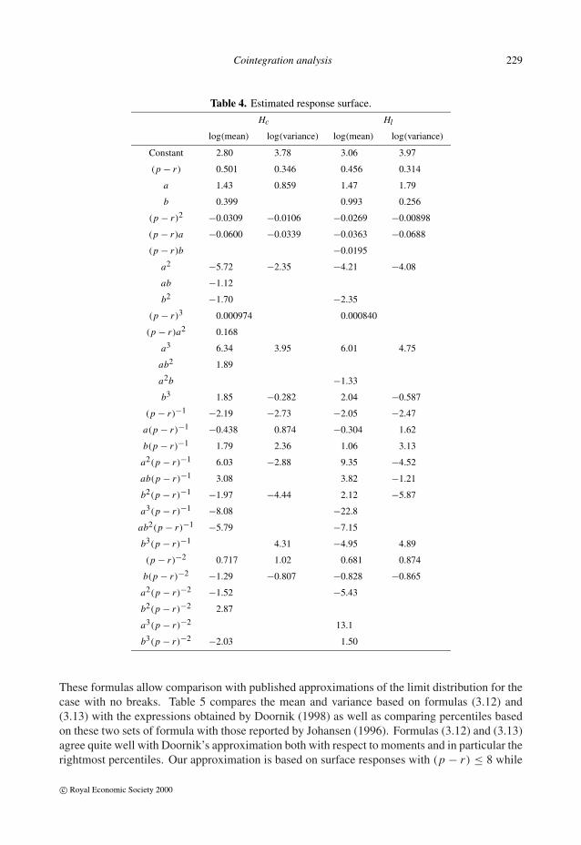
The estimated coefficients are reported in Table 4 where the coefficients referred to the variablex4 = T −1 are not reported, since they are irrelevant for computing the asymptotic moments.

In the case of q = 2 sample periods instead of q = 3 the mean and variance can still becomputed by using (3.11) by letting b = 0 and subtracting the mean and variance of a χ2(p − r)

variable, see (3.5). In the case of just q = 1 sample period let a = b = 0 and subtract anadditional χ2(p − r) variable. Thus for q = 1, 2, 3 we have the approximation

mean ≈ exp{ fmean(p − r, a, b, ∞)} − (3 − q)(p − r) (3.12)

variance ≈ exp{ fvariance(p − r, a, b, ∞)} − 2(3 − q)(p − r). (3.13)



Table 4. Estimated response surface.

Hc Hl

log(mean) log(variance) log(mean) log(variance)

Constant 2.80 3.78 3.06 3.97

(p − r) 0.501 0.346 0.456 0.314

a 1.43 0.859 1.47 1.79

b 0.399 0.993 0.256

(p − r)2 −0.0309 −0.0106 −0.0269 −0.00898

(p − r)a −0.0600 −0.0339 −0.0363 −0.0688

(p − r)b −0.0195

a2 −5.72 −2.35 −4.21 −4.08

ab −1.12

b2 −1.70 −2.35

(p − r)3 0.000974 0.000840

(p − r)a2 0.168

a3 6.34 3.95 6.01 4.75

ab2 1.89

a2b −1.33

b3 1.85 −0.282 2.04 −0.587

(p − r)−1 −2.19 −2.73 −2.05 −2.47

a(p − r)−1 −0.438 0.874 −0.304 1.62

b(p − r)−1 1.79 2.36 1.06 3.13

a2(p − r)−1 6.03 −2.88 9.35 −4.52

ab(p − r)−1 3.08 3.82 −1.21

b2(p − r)−1 −1.97 −4.44 2.12 −5.87

a3(p − r)−1 −8.08 −22.8

ab2(p − r)−1 −5.79 −7.15

b3(p − r)−1 4.31 −4.95 4.89

(p − r)−2 0.717 1.02 0.681 0.874

b(p − r)−2 −1.29 −0.807 −0.828 −0.865

a2(p − r)−2 −1.52 −5.43

b2(p − r)−2 2.87

a3(p − r)−2 13.1

b3(p − r)−2 −2.03 1.50

These formulas allow comparison with published approximations of the limit distribution for thecase with no breaks. Table 5 compares the mean and variance based on formulas (3.12) and(3.13) with the expressions obtained by Doornik (1998) as well as comparing percentiles basedon these two sets of formula with those reported by Johansen (1996). Formulas (3.12) and (3.13)agree quite well with Doornik’s approximation both with respect to moments and in particular therightmost percentiles. Our approximation is based on surface responses with (p − r) ≤ 8 while



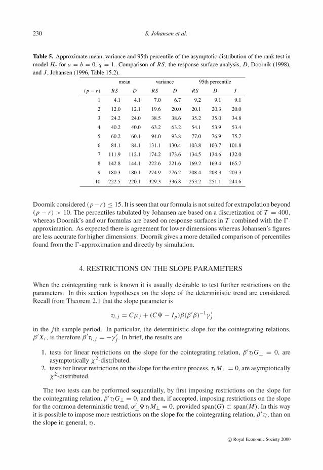
Table 5. Approximate mean, variance and 95th percentile of the asymptotic distribution of the rank test inmodel Hc for a = b = 0, q = 1. Comparison of RS, the response surface analysis, D, Doornik (1998),and J , Johansen (1996, Table 15.2).

mean variance 95th percentile

(p − r) RS D RS D RS D J

1 4.1 4.1 7.0 6.7 9.2 9.1 9.1

2 12.0 12.1 19.6 20.0 20.1 20.3 20.0

3 24.2 24.0 38.5 38.6 35.2 35.0 34.8

4 40.2 40.0 63.2 63.2 54.1 53.9 53.4

5 60.2 60.1 94.0 93.8 77.0 76.9 75.7

6 84.1 84.1 131.1 130.4 103.8 103.7 101.8

7 111.9 112.1 174.2 173.6 134.5 134.6 132.0

8 142.8 144.1 222.6 221.6 169.2 169.4 165.7

9 180.3 180.1 274.9 276.2 208.4 208.3 203.3

10 222.5 220.1 329.3 336.8 253.2 251.1 244.6

Doornik considered (p−r) ≤ 15. It is seen that our formula is not suited for extrapolation beyond(p − r) > 10. The percentiles tabulated by Johansen are based on a discretization of T = 400,

whereas Doornik’s and our formulas are based on response surfaces in T combined with the �-approximation. As expected there is agreement for lower dimensions whereas Johansen’s figuresare less accurate for higher dimensions. Doornik gives a more detailed comparison of percentilesfound from the �-approximation and directly by simulation.

4. Restrictions on the slope parameters

When the cointegrating rank is known it is usually desirable to test further restrictions on theparameters. In this section hypotheses on the slope of the deterministic trend are considered.Recall from Theorem 2.1 that the slope parameter is

τl, j = Cµ j + (C� − Ip)β(β ′β)−1γ ′j

in the j th sample period. In particular, the deterministic slope for the cointegrating relations,β ′ Xt , is therefore β ′τl, j = −γ ′

j . In brief, the results are

1. tests for linear restrictions on the slope for the cointegrating relation, β ′τl G⊥ = 0, areasymptotically χ2-distributed.

2. tests for linear restrictions on the slope for the entire process, τl M⊥ = 0, are asymptoticallyχ2-distributed.

The two tests can be performed sequentially, by first imposing restrictions on the slope forthe cointegrating relation, β ′τl G⊥ = 0, and then, if accepted, imposing restrictions on the slopefor the common deterministic trend, α′⊥�τl M⊥ = 0, provided span(G) ⊂ span(M). In this wayit is possible to impose more restrictions on the slope for the cointegrating relation, β ′τl , than onthe slope in general, τl .



Note that it is not straightforward to do these two tests in the opposite order. In that case thetest for slope of the common deterministic trend is burdened with nuisance parameters. This isrelated to the issue that the non-stationary trends are not uniquely defined.

4.1. Slope of the cointegrating relation

The slope for the linear trend in the cointegrating relation is given by the parameter γ. Linearrestrictions on this parameter can be formulated as

Hγ

l (r) : γ = Gϕ,

where G is a known (q×g)-matrix of rank g, where g ≤ q, and the parameter ϕ is a (g×r)-matrix.Under the hypothesis the slope for the cointegrating relations is therefore

β ′τl Et = −ϕ′G ′Et .

As an example suppose q = 2. By the choice G = (1, 0)′ the linear trend is absent in the secondperiod whereas if G = (1, 1)′ then the slope is not altered by the break. Note, that when there isno cointegration, r = 0, then γ vanishes, hence Hγ

l (0) = Hl(0).

As before the likelihood is maximized by canonical correlation analysis. The squared samplecanonical correlations of the residuals, 1 > λ

γ

1 > · · · > λγp > 0, are given by

CanCor

{�Xt ,

(Xt−1

tG ′Et

)∣∣∣∣Ft

},

and the likelihood ratio test for the hypothesis Hγ

l (r) in Hl(r) is

L R{ Hγ

l (r)∣∣ Hl(r)} = T

r∑i=1

log{(1 − λγ

i )/(1 − λi )},

see Johansen (1996, Theorem 7.2). The asymptotic distribution is as follows.

Theorem 4.1. Suppose Hγ

l (r) and Assumption 1 are satisfied. Then the likelihood ratio teststatistic for Hγ

l (r) in Hl(r) is asymptotically χ2{r(q − g)}-distributed.

The restriction on the linear term of the cointegrating vector, γ = Gϕ, could be combinedwith, for instance, a linear restriction on the cointegrating vector itself, β = Hψ, where H is aknown, full-rank, (p×h)-matrix and the parameter ψ is of dimension (h×r). The likelihood ratiotest statistic for this hypothesis is also asymptotically χ2. The degrees of freedom is {r(p − h)}if the alternative is Hγ

l (r) and {r(p − h + q − g)} if Hl(r) is the alternative.

4.2. Slope of the process

Restrictions on the slope τl for the process Xt are now studied. This slope is a linear combinationof the slope for the cointegrating relation, β ′τl = −γ ′, and that of the common deterministictrends, α′⊥�τl = α′⊥µ. Restrictions on γ were studied above and we now turn to restricting α′⊥µ.



Linear restrictions on α′⊥µ will be expressed in terms of a known (q × m)-matrix M wherem ≤ q. The formulation

Hµl (r) : µ = ζ M ′ + αδ′M ′⊥,

where ζ, δ are of dimension (p × m) and {(q − m) × r}, respectively, leaves α′µ unrestricted,whereas α′⊥µ is restricted so α′⊥µM⊥ = 0. If the slope of the cointegrating relation is restrictedcorrespondingly as β ′τl M⊥ = 0, or more generally as β ′τl G⊥ = 0 for some G satisfyingspan(G) ⊂ span(M), we have that the slope of the entire process satisfies τl M⊥ = 0.

As opposed to the concept of cointegrating relations the non-stationary trends are linearcombinations of the levels of the time series which do not cointegrate. They could be chosen invarious ways, for instance as β ′⊥ Xt or α′⊥� Xt . Under the above restriction, Hµ

l , the slope of theformer of these is

β ′⊥τl = β ′⊥Cζ M ′ + β ′⊥C�β(β ′β)−1γ ′,showing that restrictions on γ are necessary to interpret Hµ

l in terms of the non-stationary trends.In the following we therefore discuss likelihood ratio tests for

Hγµ

l (r) : γ = Gϕ, µ = ζ M ′ + αδ′M ′⊥in Hγ

l (r) and Hl(r). Note, that in the unrestricted model, with up to p cointegrating relations,the hypothesis Hγµ

l (p) entails no restrictions as compared with Hγ

l (p). The squared samplecanonical correlations, 1 > λ

γµ

1 > · · · > λγµp > 0, are now based on

CanCor

�Xt ,

Xt−1

tG ′Et

M ′⊥Et

∣∣∣∣∣∣Fµt

, (4.1)

where the notation Fµt indicates that the regressor Et is replaced by M ′Et . The likelihood ratio

test statistics for Hγµ

l (r) are

L R{ Hγµ

l (r)∣∣ Hγ

l (r)} = Tp∑

i=r+1

log{(1 − λγ

i )/(1 − λγµ

i )},

L R{ Hγµ

l (r)∣∣ Hl(r)} = L R{ Hγµ

l (r)∣∣ Hγ

l (r)} + L R{ Hγ

l (r)∣∣ Hl(r)},

see Johansen (1996, Theorem 6.2), where it is explained that it is convenient to express the firstof these statistics in terms of the small eigenvalues, using the fact that Hγµ

l (p) = Hγ

l (p).For the asymptotic analysis the restriction span(G) ⊂ span(M) is crucial for avoiding nuisance

parameters.

Theorem 4.2. Suppose Hγµ

l (r) and Assumption 1 are satisfied. If in addition span(G) ⊂span(M) then L R{ Hγµ

l (r)∣∣ Hγ

l (r)} and L R{ Hγµ

l (r)∣∣ Hl(r)} are asymptotically χ2-distributed

with {(p − r)(q − m)} and {(p − r)(q − m) + r(q − g)} degrees of freedom, respectively.If span(G) �⊂ span(M), the asymptotic distributions of the test statistics involve nuisance

parameters.

5. Empirical Illustration

This section illustrates the suggested statistical analysis, applied to a five-dimensional data set withvariables relevant for analysing the Uncovered Interest Parity (UIP) hypothesis between Germany



Table 6. Maximum lag analysis (p-value for the Godfrey test).

k Akaike Hannan–Quinn Schwartz Godfrey χ2ar5(125)

1 −53.63 −53.00 −52.06 0.001

2 −54.29 −53.26 −51.72 0.261

3 −54.37 −52.93 −50.80 0.231

4 −54.46 −52.62 −49.89 0.758

5 −54.80 −52.56 −49.24 0.846

and Italy. The economic model is very simple, and should be regarded as an illustration rather thana contribution to the ongoing economic debate. The analysis has been done using MALCOLM2.4 (Mosconi1998), where all the techniques illustrated in this paper are implemented in a userfriendly menu driven environment.

Let us consider the vector

Yt = (�pIt , �pD

t , �et+1, i It , i D

t )

where �pIt and �pD

t are first differences of log Consumer Price Index and represent inflation ratesin Italy and Germany. The variable �et+1 is the first differences of log nominal exchange ratebetween Italian Lira and German Mark (LIT/DM) and represents the rational expectation to futureexchange rates. Finally, i I

t and i Dt are Italian and German nominal interest rates on long-term

treasury bonds, given as annual rates divided by 4, to make them dimensionally matching withthe other variables. As for the sources, prices are from EUROSTAT (except 1973–1975, whereprices are from UN–Monthly Bulletin of Statistics); note that, after October 1990, German pricesrefer to unified Germany. Exchange Rates are from the Bank of Italy (average quarterly exchangerates). Interest Rates are from IMF, International Financial Statistics. The data are available fromthe Econometrics Journal website.

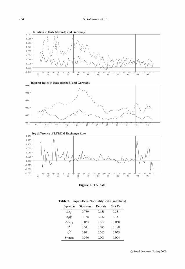
The data, which are shown in Figure 2, are quarterly, ranging from 1973.2 to 1995.4 (T = 91).To model these data, based on prior knowledge of relevant historical events, we introduce twobreaks. The last observation of the first period is 1979.4, while the last observation of the secondperiod is 1992.2 (T1 = 27, T2 = 77; v1 = 0.297, v2 = 0.846; a = 0.154, b = 0.297). The firstbreak coincides with the creation of the EMS, but it is also supposed to catch the oil shock andthe modification of the US monetary policy. The second break corresponds to the exit of Italyfrom the EMS, but also to the unification of Germany. The plot clearly shows the presence oftrends: the trend in inflation and interest rates in both countries in the second period is apparent,but one might suspect trends in some of the variables also in the first and third period. Thissuggests modelling the data using model Hl . In fact, the presence of trends in the variables maybe explained within model Hc only by random walks, whereas model Hl allows for interpretingtrends either as related to random walks or trend stationarity. Within model Hl , the nature of thetrend may be decided according to appropriate tests once the cointegration rank is determined ina setting which is robust with respect to trend stationarity.

The analysis to determine the maximum lag k is reported in Table 6. The information criteriasuggest different values of k, in which case it is common practice to prefer the Hannan–Quinncriterion. Therefore, k = 2 has been selected, since it is also the first lag to give approximatelywhite noise residuals, according to the Godfrey test.

Jarque–Bera normality tests, reported in Table 7, show some problems with skewness in the



Inflation in Italy (dashed) and Germany

73 75 77 79 81 83 85 87 89 91 93 95−0.008

0.000

0.008

0.016

0.024

0.032

0.040

0.048

0.056

0.064

Interest Rates in Italy (dashed) and Germany

73 75 77 79 81 83 85 87 89 91 93 950.01

0.02

0.03

0.04

0.05

0.06

log difference of LIT/DM Exchange Rate

73 75 77 79 81 83 85 87 89 91 93 95−0.075

−0.050

−0.025

0.000

0.025

0.050

0.075

0.100

0.125

0.150

Figure 2. The data.

Table 7. Jarque–Bera Normality tests (p-values).

Equation Skewness Kurtosis Sk + Kur

�pIt 0.789 0.155 0.351

�pDt 0.188 0.152 0.151

�et+1 0.053 0.162 0.058

i It 0.541 0.085 0.188

i Dt 0.941 0.015 0.053

System 0.376 0.001 0.004



Table 8. Rank tests.

Hypothesis Test p-value

r = 0 256.46 0.000

r ≤ 1 157.43 0.000

r ≤ 2 71.96 0.043

r ≤ 3 29.50 0.621

r ≤ 4 10.42 0.745

Table 9. Characteristic roots of the models.

Root r = 5 r = 3

1 0.82 1.00

2 0.12 + 0.72i 1.00

3 0.12 − 0.72i 0.11 − 0.71i

4 0.67 + 0.12i 0.11 + 0.71i

5 0.67 − 0.12i 0.45 − 0.27i

�et equation and kurtosis in the i Dt equation, so that, at the system level, normality is rejected. Due

to the illustrative aim of this analysis we did not try to analyse these problems any further. Note,however, that all residual-based misspecification tests, like Godfrey and Jarque–Bera, should bemodified in the present setting to take into account that the first k residuals of each period are setto zero by the presence of the dummies D j,t−i , whose purpose is to condition upon the first kobservations of each period. This might partly explain the problems with kurtosis.

Coming to cointegration analysis, UIP implies that

i It − {i D

t + Et (�et+1)} = 0 (5.1)

so that for an Italian investor the return from investing in Italy equals the expected return frominvesting in Germany. The interpretation of the relation in the context of a vector autoregressivemodel is

i It − (i D

t + �et+1) = zero mean stationary. (5.2)

Therefore, the cointegration rank r is expected to be at least equal to one, but of course it may behigher, since we do not have theoretical reasons to exclude more stationarity in the data.

The tests for cointegration rank are reported in Table 8. The analysis supports r = 3, whichis consistent with our prior expectation. Therefore, we estimate the model with r = 3. Table9 reports the five largest characteristic roots for both the unrestricted and the restricted models,which seem to be consistent with the I(1) assumption rank (α′⊥�β⊥) = (p − r).

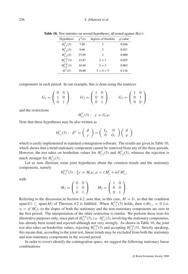
Before trying to set up identifying restrictions on the cointegration space, let us illustratesome interesting tests on the deterministic components. The slopes of the deterministic trends forthe cointegrating relations are given by the elements of the (3 × 3)-matrix γ , whose i th columnrepresents the trend coefficients of the i th stationary relation in the three different periods. Asuggested ‘routine’ analysis consists in testing for the exclusion of the linear trend in the stationary



Table 10. Test statistics on several hypotheses, all tested against Hl (r).

Hypothesis χ2(n) degrees of freedom p-value

Hγl,1(3) 7.98 3 0.046

Hγl,2(3) 9.66 3 0.021

Hγl,3(3) 27.05 3 0.000

Hγµl,1 (3) 12.87 2 + 3 0.025

Hγµl,2 (3) 10.48 2 + 3 0.063

H I (3) 18.00 3 + 4 + 5 0.116

components in each period. In our example, this is done using the matrices

G1 = 0 0

1 00 1

, G2 =

1 0

0 00 1

, G3 =

1 0

0 10 0

and the restrictionsHγ

l,i (3) : γ = Giϕ.

Note that these hypotheses may be also written as

Hγ

l,i (3) : βγ =(

β

γ

)=

(Ip 00 Gi

) (β

ϕ

)

which is easily implemented in standard cointegration software. The results are given in Table 10,which shows that a trend stationary component cannot be removed from any of the three periods.However, the test takes on borderline values for Hγ

l,1(3) and Hγ

l,2(3), whereas the rejection ismuch stronger for Hγ

l,3(3).Let us now illustrate some joint hypotheses about the common trends and the stationary

components, namelyHγµ

l,i (3) :{γ = Miϕ, µ = ζ M ′

i + αδ′M ′i⊥

with

M1 = 0 0

1 00 1

M2 =

1 0

0 00 1

.

Referring to the discussion in Section 4.2, note that, in this case, M = G, so that the conditionspan(G) ⊂ span(M) of Theorem 4.2 is fulfilled. When Hγµ

l,1 (3) holds, then τl M1⊥ = 0 (i.e.τl = ψ ′M ′

1), so the slopes of both the stationary and the non-stationary components are zero inthe first period. The interpretation of the other restriction is similar. We perform these tests forillustrative purposes only, since part of Hγµ

l,i (3), i.e. Hγ

l,i (3), involving the stationary components,has already been tested and rejected although not very strongly. As shown in Table 10, the jointtest also takes on borderline values, rejecting Hγµ

l,1 (3) and accepting Hγµ

l,2 (3). Strictly speaking,this means that, according to the joint test, linear trends may be excluded from both the stationaryand non-stationary components in the second period.

In order to (over)-identify the cointegration space, we suggest the following stationary linearcombinations



z1t = i It − (i D

t + �et+1)

z2t = (i Dt − �pD

t )

z3t = (i It − �pI

t ) − (i Dt − �pD

t ).

The equations represent the UIP hypothesis, the German real interest rate, and the real interestrate differential, respectively. Note that, if these linear combinations are stationary, then also

z4t = z1t − z3t = (�pIt − �pD

t ) − �et+1

z5t = z2t + z3t = (i It − �pI

t )

are stationary, and could be used to find an alternative and equivalent basis of the cointegrationspace. Identifying restrictions may be written as

H I (3) : βγ =(

β

γ

)= (B1b1, B2b2, B3b3).

In order to test the local trend stationarity of z1t ,z2t and z3t , together with some plausiblerestrictions on the deterministic part, we set up the following identifying restrictions:

B1 =

0 0 00 0 0

−1 0 01 0 0

−1 0 00 1 00 0 00 0 1

, B2 =

0 0−1 00 00 01 00 00 00 1

, B3 =

−1101

−1000

which exclude the linear trend from z1t in the second period, from z2t in the first and secondperiods, and from z3t in all periods. The degrees of freedom for testing H I (r) against H(r)

are given by∑r

j=1(p + q − r − dim B j + 1), see Johansen (1996, Theorem 7.5). As shown

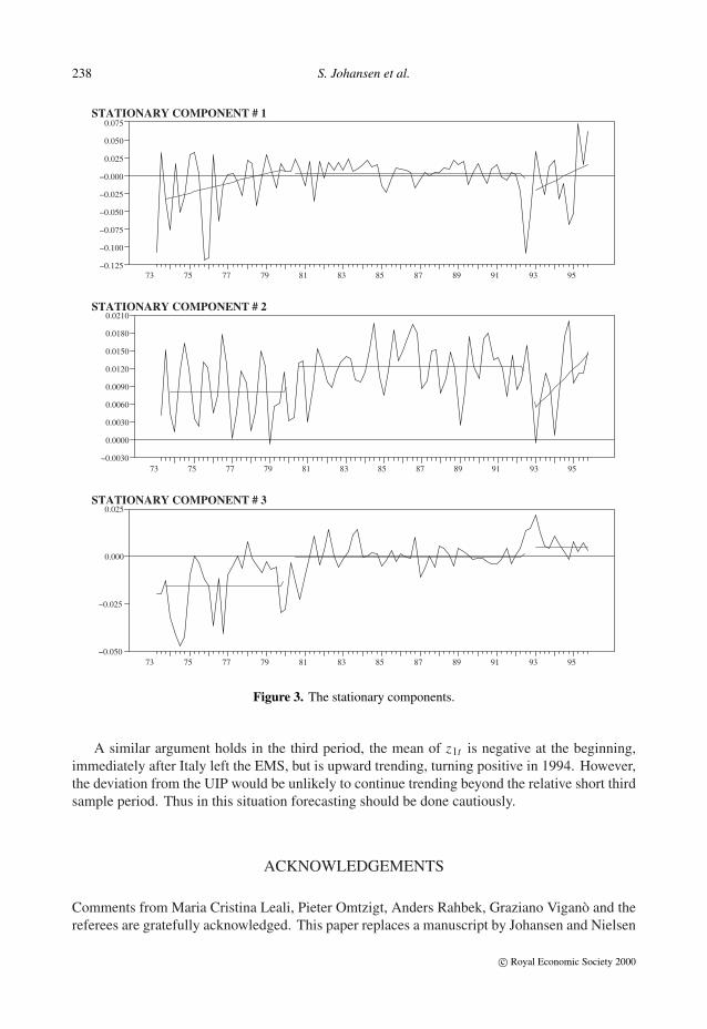
in Table 10, H I (3) cannot be rejected. Figure 3 represents z1t , z2t and z3t , together with theirdeterministic components estimated under H I (3).

This shows that in the period (79.1, 92.2), in which Italy belonged to the EMS, z1t is ap-proximately zero on average, which is evidence in favour of the UIP in that period. Conversely,the mean of z1t is negative and quite large in the first period, although trending towards zero.This means that the interest rate in Italy was much lower than predicted by UIP plus rationalexpectations. An interpretation could be that the extreme devaluation of Italian Lira in the 1970swas unexpected, or in other words (5.2) should be replaced in the first period by

i It − (i D

t + �et+1) = zero mean stationary + ρt ,

where ρt represents a systematic bias in expectations. An alternative interpretation of the lowItalian interest rate could be related to the presence of a negative risk premium on Italy: if Italyis perceived as less risky than Germany, then i I

t should be lower than (i Dt + �et+1). However,

this interpretation seems implausible in the 1970s.



STATIONARY COMPONENT # 1

73 75 77 79 81 83 85 87 89 91 93 95−0.125

−0.100

−0.075

−0.050

−0.025

−0.000

0.025

0.050

0.075


73 75 77 79 81 83 85 87 89 91 93 95−0.0030

0.0000

0.0030

0.0060

0.0090

0.0120

0.0150

0.0180

0.0210


73 75 77 79 81 83 85 87 89 91 93 95−0.050

−0.025

0.000

0.025

Figure 3. The stationary components.

A similar argument holds in the third period, the mean of z1t is negative at the beginning,immediately after Italy left the EMS, but is upward trending, turning positive in 1994. However,the deviation from the UIP would be unlikely to continue trending beyond the relative short thirdsample period. Thus in this situation forecasting should be done cautiously.

Acknowledgements

Comments from Maria Cristina Leali, Pieter Omtzigt, Anders Rahbek, Graziano Vigano and thereferees are gratefully acknowledged. This paper replaces a manuscript by Johansen and Nielsen



from 1993 with the title ‘Asymptotics for cointegration rank tests in the presence of interventiondummies – manual for the simulation program DisCo’.

REFERENCES

Anderson, T. W. (1951). Estimating linear restrictions on regression coefficients for multivariate normaldistributions. Annals of Mathematical Statistics 22, 327–351. Correction in Annals of Statistics 8, 1400(1980).

Bartlett, M. S. (1938). Further aspects of the theory of multiple regression. Proceedings of the CambridgePhilosophical Society 34, 33–40.

Chan, N. H., and C. Z. Wei (1988). Limiting distributions of least squares estimates of unstable autoregressiveprocesses. Annals of Statistics 16, 367–410.

Clements, M. P., and D. F. Hendry (1999). Forecasting Non-stationary Economic Time Series. MIT press,Cambridge MA, USA.

Doornik, J. A., (1998). Approximations to the asymptotic distribution of cointegration tests. Journal ofEconomic Surveys 12, 573–593.

Doornik, J. A., and D. F. Hendry (1994). Modelling linear dynamic econometric systems. Scottish Journalof Political Economy 41, 1–33.

Doornik, J. A., D. F. Hendry, and B. Nielsen (1998). Inference in cointegrating models: UK M1 revisited.Journal of Economic Surveys 12, 533–572.

Hansen, H., and S. Johansen (1999). Some tests for parameter constancy in the cointegrated VAR. Econo-metrics Journal 2, 25–52.

Hansen, P. R. (2000). Structural changes in cointegrated processes. Ph. D. Thesis, University of California,San Diego.

Hendry, D. F. (1997). The econometrics of macroeconomic forecasting. Economic Journal 107, 1330–1357.Hotelling, H. (1936). Relations between two sets of variates. Biometrika 28, 321–77.Inoue, A. (1999). Tests of cointegrating rank with a trend-break. Journal of Econometrics 90, 215–237.Johansen, S. (1988). Statistical analysis of cointegration vectors. Journal of Economic Dynamics and Control

12, 231–254.Johansen, S. (1996). Likelihood-based inference in Cointegrated Vector Autoregressive Models. 2nd printing.

Oxford University Press.Johansen, S. (2000a). A small sample correction for test of hypotheses on the cointegrating vectors. To

appear in Journal of Econometrics.Johansen, S. (2000b). A Bartlett correction factor for tests on the cointegrating relations. Econometric Theory

16, 740–778.Johansen, S. (2000c). A small sample correction of the test for cointegrating rank in the vector autoregressive

model. EUI working paper ECO no. 2000/15.Krolzig, H.-M., and D. F. Hendry (2000). Computer automation of general-to-specific model selection

procedures. To appear in Journal of Economic Dynamics and Control.Kuo, B. (1998). Test for partial parameters stability in regressions with I(1) processes. Journal of Econo-

metrics 86, 337–368.Mosconi, R. (1998). MALCOLM: The Theory and Practice of Cointegration Analysis in RATS. Venice: Ca’

Foscarina. Available online at http://www.greta.it/malcolm.Nielsen, B. (1997). Bartlett correction of the unit root test in autoregressive models. Biometrika 84, 500–504.Nielsen, B., and A. Rahbek (2000). Similarity issues in cointegration models. Oxford Bulletin of Economics

and Statistics 6, 5–22.Perron, P. (1989). The great crash, the oil price shock, and the unit root hypothesis. Econometrica 57,

1361–1401. Erratum (1993) Econometrica 61, 248–249.Perron, P. (1990). Testing for a unit root in a time series with a changing mean. Journal of Business &

Economic Statistics 8, 153–162. Corrections and Extensions by Perron, P., and Vogelsang, T., 1992,Journal of Business & Economic Statistics 10, 467–470.



Rappoport, P., and L. Reichlin (1989). Segmented trends and non-stationary time series. Economic Journal99 supplement, 168–177.

Seo, B. (1998). Tests for structural change in cointegrated systems. Econometric Theory 14, 222–259.

A. Appendix: Mathematical Details

The techniques in the proofs are those of Johansen (1996)—which we in the following will refer to as(J). One major difference is that the monograph focuses on models, Hlc, where the parameters for thedeterministic terms are unrestricted under the rank hypothesis, whereas here the focus is on models, Hl ,

where the deterministic component of the process is not affected by the rank hypothesis.

A.1. Proof of Theorem 2.1

Each sub-sample can be considered separately because of the conditioning on the first k observations ineach period. Representation (2.8) therefore follows from Theorem 4.2 (J). In each period the initial valueof the stationary component is given its invariant distribution, so the stationary components of (2.8), Y j,t ,are identically distributed with zero expectation. To derive the representations for the slope parameter τl, jand the intercept parameter β ′τc, j we find from representation (2.8) for Tj−1 + k < t ≤ Tj ,

E(β ′Xt ) = β ′τc, j + β ′τl, j t, E(�Xt ) = τl, j ,

and taking expectation in (2.6) we obtain, since the dummies are zero,

τl, j = α{β ′τc, j + β ′τl, j (t − 1) + γ ′j t} + µ j +

k−1∑i=1

�i τl, j

identifying coefficients, we find for � = Ip − ∑k−1i=1 �i

�τl, j = α(β ′τc, j − β ′τl, j ) + µ j , β ′τl, j + γ ′j = 0,

or (µ jγ ′

j

)=

(� + αβ ′ −α

−β ′ 0

) (τl, j

β ′τc,t

).

The expressions in the theorem then follow by noting that(C (C� − Ip)β

α′(�C − Ip) α′(�C� − �)β − Ir

) (� + αβ ′ −α

−β ′ 0

)= Ip+r .

A.2. Some asymptotic results

The statistical analysis is based on canonical correlation analysis. It is important to note that the samplecanonical correlations are invariant with respect to linear transformations of the data, whereas the corre-sponding canonical vectors used for estimating the cointegrating vector transform linearly.

For any two processes Ut and Vt we define the residuals

(Ut |Vt ) = Ut −T∑

s=1

Us V ′s

(T∑

s=1

Vs V ′s

)−1

Vt .



We work under the assumption Hγl (r): γ = Gϕ, see Section 4.1, and define the extended parameter

βγ = (β ′, ϕ′)′. In the reduced rank problem the process (X ′t−1, t E ′

t G) enters. Since Xt exhibits a lineartrend according to Theorem 2.1 it is convenient to detrend the levels of the process using the last componentof the vector, t E ′

t G, and replace (X ′t−1, t E ′

t G) by {(Xt−1|tG′Et )′, t E ′

t G}. Thus, define

QT =(

Ip

(∑Tt=1 Xt−1 E ′

t Gt) (∑T

t=1 tG′Et E ′t Gt

)−1

0 Ig

),

so that (Xt−1tG′Et

)= QT

(Xt−1|tG′Et

tG′Et

)and hence

βγ ′(

Xt−1tG′Et

)=

(β

ϕ

)′ ( Xt−1tG′Et

)=

(Q′

T

(β

ϕ

))′ ( Xt−1|tG′EttG′Et

).

We define the residual processes

(R0,t , R1,t ) ={

�Xt ,

(Xt−1|tG′Et

tG′Et

)∣∣∣∣Ft

}(A.1)

and the residual product moment matrices

(S00 S01S10 S11

)= 1

T

T∑t=1

(R0,tR1,t

) (R0,tR1,t

)′.

Note that S11 is block diagonal because the residuals (Xt−1|tG′Et ) and tG′Et are orthogonal. The squaredsample canonical correlations, 1 ≥ λ

γ1 ≥ · · · ≥ λ

γp ≥ 0 and λ

γi = 0 say, for i = p + 1, . . . , p + g of R0

and R1 are then given as solutions to the eigenvalue problem∣∣∣λγ S11 − S10S−100 S01

∣∣∣ = 0.

The corresponding eigenvectors, vi , satisfy

S11λγi vi = S10S−1

00 S01vi .

The matrix of the r first eigenvectors is denoted β0 and the parameters β and ϕ are estimated from theequation

Q′T βγ = Q′

T

(β

ϕ

)= β0. (A.2)

A corresponding asymptotic relation can be established for the parameters using the representation inTheorem 2.1

(β0)′ =β ′,

T∑t=1

(β ′Xt−1 + tϕ′E ′t G)E ′

t Gt

(T∑

t=1

tG′Et E ′t Gt

)−1

= {β ′, OP (T −1)} P→ (β ′, 0)de f= (β0)′, (A.3)

since β ′Xt + tϕ′E ′t G is stationary.



In order to formulate the asymptotic results for the residuals in model Hγl (r) some notation is needed.

Below we will choose an {(p−r)×n}-matrix ξ with full column rank. We can then obtain three independentstandard Brownian motions of dimensions r, n, (p − r − n), respectively,

(α′�−1α)−1/2α′�−1T −1/2int(T u)∑

t=1

εtD→ Vu ,

(ξ ′ξ)−1/2ξ ′(α′⊥�α⊥)−1/2α′⊥T −1/2int(T u)∑

t=1

εtD→ Wξ,u ,

(ξ ′⊥ξ⊥)−1/2ξ ′⊥(α′⊥�α⊥)−1/2α′⊥T −1/2int(T u)∑

t=1

εtD→ Wξ⊥,u .

Further define

Wu =(

Wξ,uWξ⊥,u

), Fu =

(Wuueu

∣∣∣∣ eu

).

To motivate the choice of ξ consider the representation of X given in Theorem 2.1 and use the identityIg = G⊥G′⊥ + GG′ to find

β ′⊥Xt = β ′⊥Ct∑

i=Tj−1+k+1

εi + tβ ′⊥τl G⊥G′⊥Et + tβ ′⊥τl GG′Et + OP (1), (A.4)

for Tj−1 +k < t ≤ Tj . The residuals are found by correcting for tG′Et and the variables inFt . Since tG′Et

is eliminated by regression the residual (β ′⊥Xt |tG′Et ,Ft ) has a linear trend β ′⊥τl G⊥G′⊥(t Et |G′Et , Et ).

It turns out that the limit distribution depends on the row space of the {(p − r) × (q − g)}-matrix β ′⊥τl G⊥.

If it has rank n, say, its row space is spanned by a {(q − g)× n}-matrix η of full rank. Note that η also spansthe row space of α′⊥µG⊥.

In order to utilize the Brownian motion W in the asymptotic analysis of (A.4) we will transform thecolumn space of β ′⊥τl G⊥. By Assumption 1 the matrices α′⊥�α⊥ and α′⊥�β⊥ have full rank. Choose a

{(p − r) × n}-matrix ξ so (α′⊥�α⊥)−1/2α′⊥�β⊥β ′⊥τl G⊥ = ξη′. It follows that

(ξ ′⊥ξ⊥)−1/2ξ ′⊥(α′⊥�α⊥)−1/2α′⊥�β⊥T −1/2

{β ′⊥C

int(T u)∑t=1

εt

}D→ Wξ⊥,u .

In correspondence with this we proceed to define the directions

B1 =(

β⊥β′⊥�α⊥(α′⊥�α⊥)−1/2

0

)B2 =

(0Ig

).

These constitute an orthogonal complement of β0 = (β ′, 0)′. Finally, define

BT = {B1ξ⊥(ξ ′⊥ξ⊥)−1/2, B1ξT −1/2, B2T −1/2}.

Lemma A.1. Asymptotic properties of B′T R1. Suppose hypothesis Hγ

l (r) and Assumption 1 are satisfied.Define the matrix

N ′ = Ip−r−n 0(p−r−n)×n 0(p−r−n)×q

0n×(p−r−n) 0n×n η′G′⊥{Iq − ZG(G′ZG)−1G′}0g×(p−r−n) 0g×n G′

, (A.5)



where Z = ∫ 10 (ueu |eu)(ueu |eu)′du. Then as T → ∞

1√T

B′T R1,int(T u)

D→ Wξ⊥,u

η′G′⊥{Iq − ZG(G′ZG)−1G′}ueuG′ueu

∣∣∣∣∣∣ eu

= N ′Fu . (A.6)

If G = Iq then Hγl (r) reduces to Hl (r), g = q, n = 0 and N = Ip−r+q .

If G = 0 then Hγl (r) reduces to Hlc(r), q = 0 and N is given in Theorem 3.3.

The proof follows from (A.4). It is seen from (A.4) that the residual

ξ ′⊥(α′⊥�α⊥)−1/2α′⊥�β⊥β ′⊥(Xt |tG′Et ,Ft )

has no trend and behaves asymptotically like a random walk corrected for Et so

T −1/2(ξ ′⊥ξ⊥)−1/2ξ ′⊥B′1 Rint(T u)

D→ (Wξ⊥,u |eu). (A.7)

It also follows from (A.4) that ξ′(α′⊥�α⊥)−1/2α′⊥�β⊥β ′⊥(Xt−1|tG′Et ,Ft ) behaves asymptotically

like η′G′⊥(t Et |tG′Et , Et ) and hence

T −1ξ′B′

1 Rint(T u)D→ η′G′⊥(ueu |G′ueu , eu). (A.8)

Finally we find

T −1 B′2 Rint(T u) = T −1G′{int(T u)Eint(T u)|Fint(T u)} P→ G′(ueu |eu). (A.9)

The proof is completed by combining (A.7)–(A.9) �

For each period the processes �Xt and β ′Xt−1 + tϕ′G′Et can be given stationary initial distributions,see Theorem 2.1. Apart from a changing level the stationary distributions are identical. Thus define(

"00 "0β

"β0 "ββ

)= Var

(�Xt

β ′Xt−1 + tϕ′G′Et

∣∣∣∣ �Xt−1, . . . , �Xt−k+1

).

Lemma A.2. Asymptotic behaviour of Si j . Suppose hypothesis Hγl (r) and Assumption 1 are satisfied. Then,

as T → ∞, (S00 S01β0

β0′S10 β0′S11β0

)P→

("00 "0β

"β0 "ββ

). (A.10)

This asymptotic covariance matrix satisfies the identity

"−100 − "−1

00 "0β("β0"−100 "0β)−1"β0"−1

00 = α⊥(α′⊥�α⊥)−1α′⊥. (A.11)

The product moment matrices satisfy a joint convergence result

T −1 B′T S11 BT

D→ N ′∫ 1

0Fu F ′

uduN , (A.12)

(α′�−1α)−1/2α′�−1

(ξ ′ξ)−1/2ξ ′(α′⊥�α⊥)−1/2α′⊥(ξ ′⊥ξ⊥)−1/2ξ ′⊥(α′⊥�α⊥)−1/2α′⊥

Sε1 BT

D→∫ 1

0

(dVudWu

)F ′

u N , (A.13)

(B′T S10, B′

T S11β0) = OP (1), (A.14)

where Sε1 = S01 − αβγ ′QT S11.



The proof of equations (A.12)–(A.14) follows from Lemma A.1. Equation (A.10) follows by notingthat for Tj−1 + k < t ≤ Tj , representation (2.8) implies

�Xt = Cεt + �Y j,t + τl Et ,

β ′Xt = β ′(Y j,t + τc Et + tτl Et ) = β ′Y j,t + β ′τc Et − tϕ′G′Et ,

since the dummies are all zero. The distribution of Y j,t is the same in all periods. Consequently, theprocesses β ′Xt−1 + tϕ′G′Et and �Xt are stationary and the conditional variance, (A.10), is the same inall periods. Further,

(β ′Xt−1∣∣ tG′Et ,Ft ) = (β ′Xt−1 + tϕ′G′Et

∣∣ tG′Et ,Ft )

and hence the limit in (A.10) is expressed in terms of the variance of β ′Xt−1 + tϕ′G′Et . Finally, equation(A.11) follows from Lemma 10.1 (J).

The joint convergence of (A.12), (A.13) follows from Chan and Wei (1988). �


Under Hl (r) we have G = Ig , so n = 0, N = Ip−r+g and W = Wξ⊥ . The asymptotic result is then foundas in the proof of Theorem 11.1 (J). Note that the proof relies on identity (A.11). �


The proof resembles that of Theorem 3.1 but G = 0, so g = 0, G⊥ = Iq . The asymptotic theory thereforedepends on the n-dimensional row space of α′⊥µ.

(1) If n = (p − r) ≤ q we find N ′ = {0n×(p−r), η′} and W = Wξ . As in the proof of Theorem 3.1

we find that the asymptotic distribution is of form (3.8). Since N ′Fu = (ueu |eu) is deterministic, see (A.6),then (3.8) is χ2-distributed.

(2) If n = q < (p − r) then

N ′ =(

Ip−r−q 0 00 0 η′

)=

(Ip−r−q 0

0 η′) (

Ip−r−q 0 00 0 Iq

)

while Wu has components Wξ,u , Wξ⊥,u . Define M = {ξ(ξ ′ξ)−1/2, ξ⊥(ξ ′⊥ξ⊥)−1/2}. Result (A.13) thenimplies that

(α′⊥�α⊥)−1/2α′⊥Sε1 BTD→ M ′

∫ 1

0dWu F ′

u N .

As in the proof of Theorem 3.1 the limit distribution of L R{Hlc(r)|Hlc(p)} is

tr

M ′

∫ 1

0dWu F ′

u N

(∫ 1

0N ′Fu F ′

u Ndu

)−1 ∫ 1

0N ′FudWu M

which reduces to (3.8) since M is orthogonal. Noting that η is regular the diagonal matrices diag(Ip−r−q , η′)cancel.

(3) If n < min(q, p − r) we arrive at expression (3.8) as in case (2). �



A.5. Asymptotic properties of β under Hγl (r)

The proof of Theorem 4.1 uses the asymptotic properties of β0, see (A.2). To discuss these it is convenientto apply the normalization

β0 = β0(β0′β0)−1.

Since the matrix (β0, BT ) has full rank and orthogonal blocks, β0′BT = 0, it follows that Ip+g =β0β0′ + BT B′

T . Consequently,

β0 = β0 + BT B′T β0 = β0 + BT UT , where UT = B′

T β0.

Correspondingly, define α = αβ0′β0 so αβ0′ = αβ0′.

Lemma A.3. Asymptotic behaviour of Si j . Suppose hypothesis Hγl (r) and Assumption 1 are satisfied. Then

the estimators β0, α, and � in model Hγl (r) are consistent and

β0′S11β0 = β0′S11β0 + oP (1) β0′S10 = β0′S10 + oP (T −1/2).

Moreover, the estimator β0 is asymptotically mixed Gaussian in the sense that

T UT = B′T (β0 − β0)

D→(

N ′∫ 1

0Fu F ′

uduN

)−1

N ′∫ 1

0Fu(dVu)′(α′�−1α)−1/2,

where F and N are given by (3.3) and (A.5). Note, that V and F are independent since V and W areindependent by construction.

The proof follows those of Lemma 13.1 and 13.2 (J). ✷

In Lemma A.5 below the test for a simple hypothesis on βγ is discussed. Both of the parameters βγ andβ0 are used in the proof. Thus recall the above definition of the residual product moment matrices Si j wherethe levels of the process are detrended. Correspondingly, let Sγ

i j be the residual product moment matriceswhere the levels are not detrended, hence,(

Sγ00 Sγ

01

Sγ10 Sγ

11

)=

(Ip 00 QT

) (S00 S01S10 S11

) (Ip 00 Q′

T

).

Lemma A.4. Detrending of levels residuals. Suppose hypothesis Hγl (r) and Assumption 1 are satisfied.

Then

βγ ′Sγ10 = β0′S10, βγ ′Sγ

11βγ = β0′S11β0, (A.15)

βγ ′Sγ10 = β0′S10 + oP (1), βγ ′Sγ

11βγ = β0′S11β0 + oP (1). (A.16)

The proof. The two identities in (A.15) follow from Q′T βγ = β0, see (A.2). For (A.16) combine approxi-

mation (A.3) and Lemma A.2. For instance,

βγ ′Sγ10 = βγ ′QT S10 = (Q′

T βγ − β0)′S10 + β0′S10

where Q′T βγ − β0 is OP (T −1), see (A.3), and S10 is of stochastic order OP (T 1/2) by (A.10) and (A.14).

✷



Lemma A.5. Test for simple hypothesis on βγ in model Hγl (r). Suppose Assumption 1 and the hypothesis

are satisfied. Then

L R{βγ |Hγl (r)} D→ tr

∫ 1

0dVu F ′

u N

(N ′

∫ 1

0Fu F ′

uduN

)−1

N ′∫ 1

0FudV ′

u

.

This variable is χ2{r(p − r + g)}-distributed since V and F are independent.

The proof relies on an expansion of the likelihood functions around βγ . Using Lemma A.4 it is possibleto replace βγ , βγ and Sγ

i j with β0, β0 and Si j without changing the asymptotic results. The remainingarguments of the proof of Lemma 13.8 (J) can then be followed using Lemma A.3. The degrees of freedomis given by the product of dim V = r and dim(N ′F) = p − r + g.


Using Lemma A.5 and defining Z = ∫ 10 dVu F ′

u(∫ 1

0 Fu F ′udu)−1/2, M = (

∫ 10 Fu F ′

udu)1/2 N , the asymptoticdistribution is found to be

L R{Hγl (r)|Hl (r)} = L R{βγ |Hl (r)} − L R{βγ |Hγ

l (r)}D→ tr(Z Z ′) − tr{Z M(M ′M)−1 M ′Z ′} = tr{Z M⊥(M ′⊥M⊥)−1 M ′⊥Z ′}.

Since M is a function of W which is independent of V this variable is χ2 and independent of W. The degreesof freedom is the product of dim V = r and dim(N ′⊥F) = (q − g). �

A.7. Asymptotic results under the hypothesis Hγµl (r)

For the asymptotic analysis of Hγµl (r) the assumption span (G) ⊂ span (M) is important. Had this not been

satisfied nuisance parameters would appear. The easiest example of that phenomenon is seen in a modelwithout breaks, q = 1, one lag, k = 1, and a linear trend for the cointegrating relation, G = I1 = 1,

�Xt = α(β ′Xt−1 + γ ′t) + µ + εt .

The test for absence of the common deterministic slope, µ = αδ′ or M = 0, is burdened with nuisanceparameters.

The likelihood ratio test statistic for Hγµl (r) in Hγ

l (r) is based on the sample canonical correlationsgiven in (4.1). Due to the invariance properties of canonical correlations it is equivalent to consider canonicalcorrelations of the residuals

(Rγµ0,t , Rγµ

1,t ) =�Xt ,

Xt−1|tG′Et , M ′⊥Et

tG′Et |M ′⊥EtM ′⊥Et

∣∣∣∣∣∣Fµt

. (A.17)

HereFµt indicates that we have only corrected for M ′Et rather than for Et . Let Sγµ

i j denote the correspondingsample product moment matrices.

The sample product moment matrices Sγµi j can be expressed as

(Sγµ

00 Sγµ01

Sγµ10 Sγµ

11

)=

S00 + s01s−111 s10

(S01 s01

)(S10s10

) (S11 00 s11

) ,



where si j are the sample product moment matrices of the residuals

(r0,t , r1,t ) = (�Xt , M ′⊥Et∣∣Fµ

t ).

The expression for Sγµ00 follows because the regressor set Fµ

t is smaller than Ft . Further, the first two

components of Rγµ1,t are orthogonal to the last component giving the orthogonal structure of Sγµ

11 and canbe represented as (

Xt−1|tG′EttG′Et

∣∣∣∣ M ′⊥Et ,Fµt

)=

(Xt−1|tG′Et

tG′Et

∣∣∣∣Ft

)= R1,t ,

see (A.1), implying that the upper left blocks of Sγµ11 , Sγµ

10 are S11, S10. The asymptotic properties of Si jare given in Lemma A.2 and we only need to describe si j .

Lemma A.6. Asymptotics for si j . Suppose hypothesis Hγµl (r), Assumption 1 and the condition span(G) ⊂

span(M) are satisfied. Define the (q − m)-dimensional function fu = M ′⊥(eu |M ′eu). For T → ∞ thefollowing results hold jointly with those in Lemma A.2

T 1/2s01 = OP (1), (A.18)

s11P→

∫ 1

0fu f ′

udu, (A.19)

T 1/2s10α⊥(α′⊥�α⊥)−1/2 D→∫ 1

0fudW ′

u . (A.20)

It then follows that Sγµ00

P→ "00 and hence

(Sγµ00 )−1 − (Sγµ

00 )−1Sγµ01 βµ{βµ′Sγµ

10 (Sγµ00 )−1Sγµ

01 βµ}−1βµ′Sγµ10 (Sγµ

00 )−1

P→ α⊥(α′⊥�α⊥)−1α′⊥, (A.21)

where βµ is the {(p + g + q − m) × r}-matrix (β ′, 0)′.When span(G) �⊂ span(M) and the slope parameter satisfies τl M⊥ �= 0, then s01 = OP (1) and the

limit in (A.21) involves nuisance parameters.

For the proof the main observation is that for a stationary process, Zt , with zero mean and finite varianceand adapted to the natural filtration for εt

T∑t=1

Et E ′t = O(T ),

T∑t=1

Et Z ′t = OP (T 1/2),

T∑t=1

Zt−1εt = OP (T 1/2). (A.22)

In order to use those results the differenced process needs to be analysed carefully. Theorem 2.1 and Hγµl

imply the representation�Xt = Cεt + �Yt Et + τl Et ,

whereτl = Cζ M ′ + (C� − Ip)βϕ′G′.

If span(G) ⊂ span(M) then G′M⊥ = 0 and τl = θ M ′ for some parameter θ and

(�Xt | M ′Et ) = (Cεt + �Yt Et | M ′Et ). (A.23)

(A.19): For the asymptotic analysis of s11 the regression on lagged differences can be ignored becauseof (A.22), (A.23), hence

s11 = T −1T∑

t=1

( M ′⊥Et∣∣ M ′Et , D j,t−i )( M ′⊥Et

∣∣ M ′Et , D j,t−i )′ + oP (1). (A.24)



For asymptotic purposes the regression on the dummies also can be ignored and (A.19) follows.(A.18): For the analysis of s10 note that (A.23) implies that

s10 = T −1T∑

t=1

(M ′⊥Et )(Cεt + �Yt Et | M ′Et , Cεt−i + �Yt−i Et−i , D j,t−i )′. (A.25)

Then (A.22) shows that T 1/2s10 = OP (1).

(A.20): The model equation (2.6) implies that (α′⊥�Xt∣∣Fµ

t ) = (α′⊥εt∣∣Fµ

t ). Using (A.22), (A.23) asabove it follows that

T 1/2s10α⊥ = T −1/2T∑

t=1

(M ′⊥Et )(α′⊥εt∣∣ M ′Et , D j,t−i )

′ + oP (1), (A.26)

and this leads to (A.20).(A.21): Since s10 = OP (T −1/2) while S00, s11 are of order one, then Sγµ

00 = S00 + oP (1). Using that

βµ′Sγµ10 = β0′S10 it then follows that

(Sγµ00 )−1 − (Sγµ

00 )−1Sγµ01 βµ{βµ′Sγµ

10 (Sγµ00 )−1Sγµ

01 βµ}−1βµ′Sγµ10 (Sγµ

00 )−1

= S−100 − S−1

00 S01β0(β0′S10S−100 S01β0)−1β0′S10S−1

00 + oP (1)

which by (A.10), (A.11) converges to α⊥(α′⊥�α⊥)−1α′⊥.

When τl M ′⊥ �= 0 then span(G) �⊂ span(M) and β ′τl M ′⊥ �= 0. Result (A.23) then fails and s10 is oforder one. In particular, β ′s01 = β ′τl s11 + oP (1) converges to a non-zero value. �


Suppose span(G) ⊂ span(M). The proof follows in two steps. First it is established that the likelihood ratiotest statistic for Hγµ

l (r) against Hγµl (p) = Hγ

l (p) converges in distribution to

tr

∫ 1

0dWu

(N ′Fu

fu

)′ {∫ 1

0

(N ′Fu

fu

) (N ′Fu

fu

)′du

}−1 ∫ 1

0

(N ′Fu

fu

)dWu

′ ,

where f is defined in Lemma A.6. The proof is the same as that of Theorem 3.1 with BT replaced by

BγµT =

(BT 00 T 1/2 Iq−m

).

The same type of argument shows that the likelihood ratio test statistic for Hγl (r) against Hγ

l (p) convergesin distribution to

tr

∫ 1

0dWu F ′

u N

(∫ 1

0N ′Fu F ′

u Ndu

)−1 ∫ 1

0N ′FudWu

′ .

Since F and f are orthogonal we find

L R{Hγµl (r)|Hγ

l (r)} = L R{Hγµl (r)|Hγ

l (p)} − L R{Hγl (r)|Hγ

l (p)}D→ tr

∫ 1

0dWu f ′

u

(∫ 1

0fu f ′

udu

)−1 ∫ 1

0fudWu

′

which is χ2 with dimW = (p − r) times dim f = (q − m) degrees of freedom.



For the joint test we use

L R{Hγµl (r)|Hl (r)} = L R{Hγµ

l (r)|Hγl (r)} + L R{Hγ

l (r)|Hl (r)}.

From the proof of Theorem 4.1 we have that L R{Hγl (r)|Hl (r)} is asymptotically χ2 and independent of W.

The asymptotic distribution of L R{Hγµl (r)|Hl (r)} is therefore a sum of two independent χ2-distributions.

If span(G) �⊂ span(M) then (A.21) fails and the above arguments do not hold. It follows that nuisanceparameters are involved in the asymptotic distributions.


Johansen Et Al-2000-The Econometrics Journal

Documents

Transcript of Johansen Et Al-2000-The Econometrics Journal