Joe’s Relatively Small Book

of Special Relativity

Joseph Minahan c©

This page intentionally left blank

2

Special Relativity Notes

Preface

In the fall of 2006 I had been asked by several students if I knew a good book toread about tensors. I am sure that they exist, but I could not immediately think of any.So a week before the exam I quickly wrote up 8 pages of notes summarizing what wasdiscussed in class concerning tensors. I called it Tensors without tears. The followingyear I added about 4 more pages explaining many examples of tensors.

The students seemed to like the notes, or at least that is what they claimed in theevaluations. But many students also said that they did not like the book, either because itwas too compressed, or it was too expensive, or sometimes because it was too compressedand too expensive. In fact, my guess is that less than half the students even botheredto buy the book. For several years myself and others have been looking for a suitablesubstitute, but so far the books that we have found are too elementary for this particularcourse. In particular, the course is supposed to cover some topics in electromagnetism,but the usual introductory books on special relativity don’t address this subject.

Having given up trying to persuade the students to buy the book, I have decided tobite the bullet and type up some notes relevant for the whole course. However, the notesare intended to complement the book and I still recommend its purchase.

List of changes:

• September 2011: Added a new section (8) about the Lagrangian and Hamiltonianformalism for relativistic particles.

3

1 Introduction

Special relativity is relevant in physics when the speed of an object is less than, but of thesame order of magnitude as the speed of light. In this course, we will always refer to thisspeed as c, where c ≈ 2.99× 108 m/sec. In fact, we will almost always approximate thisas c = 3× 108 m/sec. If we consider a car traveling on the motorway at a speed of 100km/hr, Galilean-Newtonian mechanics is more than adequate to describe its motion. Onthe other hand, for protons circling in the now completed LHC (Large Hadron Collider)at CERN, special relativity will be particularly important.

In this course we will almost always be concerned with classical physics withoutgravity. The modern definition of classical physics means that we ignore quantum effects.Introducing gravity modifies special relativity to General Relativity, but unfortunatelythat is beyond the scope of this course.

Before we see what special relativity is, let us recall how we treat classical physics inthe Newtonian-Galilean fashion. Our primary concern is the measurement of positions,times, velocities momenta etc. of particles. One of the main things we need to consideris the position of a particle at a particular time. A time combined with a position will becalled an event. An event could mean the time and position where an explosion occurred,or the time and position of a particle at some particular point on its trajectory. Thetrajectory itself is made up of an infinite number of events as the particle travels throughtime and space. In any case, an event is described by a point in space-time. We canexpress this point by the four numbers

(t0, x0, y0, z0), (1.1)

where the first number refers to the time and the other three refer to the spatial coor-dinates. We will often measure these four quantities for various events, which can occurover a four-dimensional space-time coordinate system

(t, x, y, z) , (1.2)

which we will sometimes write as(t, ~x) . (1.3)

These coordinates are often measured in a lab, so we will sometimes refer to a coordinatesystem as a lab. But the name we will mainly use is reference frame, which we will denotein bold-face as S. The person making these measurements in a particular reference framewill be referred to as an observer. The reference frame for a particular observer is oftencalled the observer’s rest frame. In fact, we will often refer to the rest frames of bodiesor particles, that is, the reference frame where that particular body or particle is at rest.

In this class we will be mainly concerned with a particular type of reference frame,called an inertial frame. An inertial frame is a reference frame with the following prop-erties:

1. There is a universal time coordinate that can be synchronized everywhere in theinertial frame. This means is that at every spatial point in the reference frame wecan place a clock and that all the clocks agree with each other.

4

2. Euclidean spatial components. This means that the spatial components satisfy allaxioms of Euclidean geometry.

3. A body with no forces acting on it will travel at constant velocity according to theclocks and measuring sticks in the inertial frame.

An important part of this course is determining what different observers measure. Inparticular, different observers can be in different reference frames. Let us suppose thatyou are on the side of a motorway in reference frame S. Another observer who is passingby in a Volvo traveling at velocity ~v is in a different reference frame S′. The frame S′

has a different set of coordinates (t′, x′, y′, z′) and uses these coordinates to measure thespace-time positions of events. An important question is how do the coordinates in S′

relate to those in S? For example suppose that as the car is passing the observer on theside of the road with velocity ~v it also has a constant acceleration ~a. What we havepreviously learned in physics is that the times in S and S′ are the same, that is

t′ = t . (1.4)

The positions are related by

~x = ~x ′ +1

2~a t2 + ~v t+ ~x0, (1.5)

where ~x0 is independent of time.Let us consider the special case where ~a = 0, in other words, the two frames are

moving at a constant velocity with respect to each other. In this case the transformationbetween the two sets of coordinates is known as a Galilean transformation. It also meansthat if S is an inertial frame then S′ is also an inertial frame. It will often be the casethat the times and positions that we measure are between two space-time points. Thedisplacement between these two points (t1, ~x1) and (t2, ~x2) is given by

(∆t,∆~x) = (t2 − t1, ~x2 − ~x1) . (1.6)

The displacement in S′, is then given by the Galilean transformation

(∆t′,∆~x ′) = (∆t,∆~x− ~v∆t) , (1.7)

and the inverse transformation, that is the transformation that takes us back to thecoordinates in S is

(∆t,∆~x) = (∆t′,∆~x ′ + ~v∆t′) . (1.8)

One advantage of considering the displacement between two events as opposed to thespace-time position of one event is that the constant vector ~x0 drops out.

Let us now consider the velocity of a body measured by two observers in differentreference frames. Again suppose that the Volvo is moving with constant velocity ~v.Hence the velocity of frame S′ with respect to1 S is ~v. Let us further suppose that the

1The expression with respect to will be used all the time, so to save space we will often abbreviatethis as wrt.

5

body inside the Volvo is moving with a velocity ~u ′ as measured by an observer in thecar. If ~u ′ is constant, then in order to measure the body’s velocity the observer needsto determine two space-time points (events) in the body’s trajectory. Let us assumethat the displacement between these two events is (∆t′,∆~x ′). The observer in S′ thencomputes the velocity of the body to be

~u ′ =∆~x ′

∆t′. (1.9)

The observer in frame S (the one at the side of the road) would measure a differentvelocity ~u, which is found by using the inverse Galilean transformation in (1.8). Hencethe velocity this observer measures is

~u =∆~x

∆t=

∆~x ′ + ~v∆t′

∆t′= ~u ′ + ~v . (1.10)

Hence we see that to find the velocity in S all we do is add ~v to the velocity measuredin S′. This addition of velocities appears to be almost trivial so why are we worryingabout it? The reason is that this rule for the addition of velocities is violated in nature!

1.1 The Michelson-Morley experiment

Let’s assume that the Galilean addition of velocity rule is the correct one. This meansthat if an observer in S′ measures ~u ′ for a velocity, then an observer in S measures~u = ~u ′ + ~v. One velocity we could choose to measure is that of a wave, say of a soundwave, a water wave, or even a light wave.

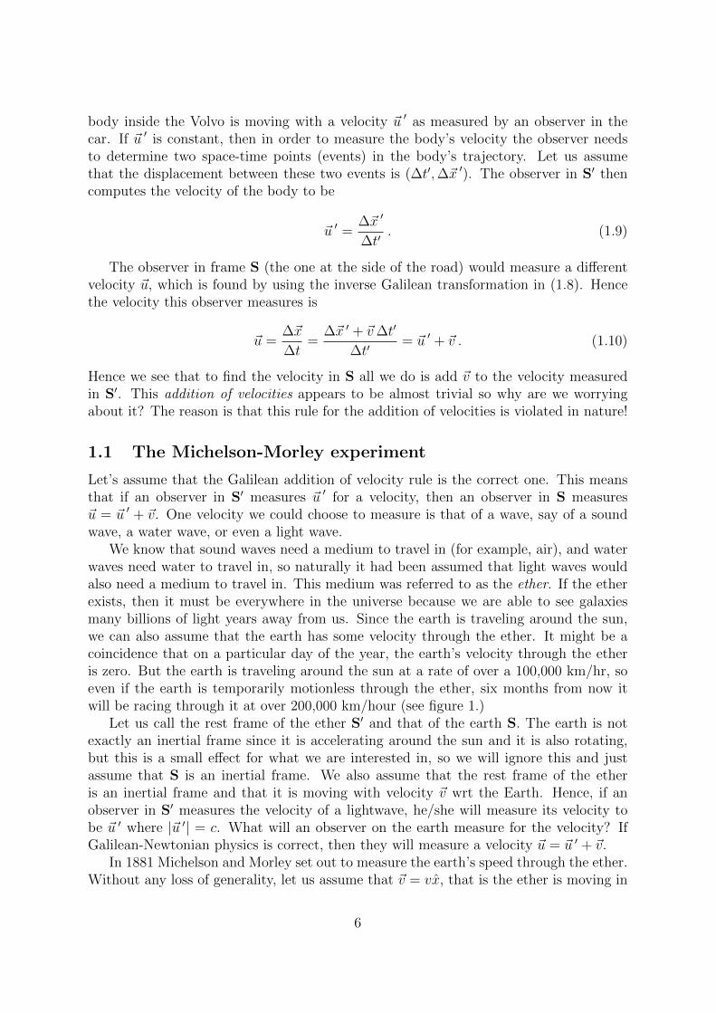
We know that sound waves need a medium to travel in (for example, air), and waterwaves need water to travel in, so naturally it had been assumed that light waves wouldalso need a medium to travel in. This medium was referred to as the ether. If the etherexists, then it must be everywhere in the universe because we are able to see galaxiesmany billions of light years away from us. Since the earth is traveling around the sun,we can also assume that the earth has some velocity through the ether. It might be acoincidence that on a particular day of the year, the earth’s velocity through the etheris zero. But the earth is traveling around the sun at a rate of over a 100,000 km/hr, soeven if the earth is temporarily motionless through the ether, six months from now itwill be racing through it at over 200,000 km/hour (see figure 1.)

Let us call the rest frame of the ether S′ and that of the earth S. The earth is notexactly an inertial frame since it is accelerating around the sun and it is also rotating,but this is a small effect for what we are interested in, so we will ignore this and justassume that S is an inertial frame. We also assume that the rest frame of the etheris an inertial frame and that it is moving with velocity ~v wrt the Earth. Hence, if anobserver in S′ measures the velocity of a lightwave, he/she will measure its velocity tobe ~u ′ where |~u ′| = c. What will an observer on the earth measure for the velocity? IfGalilean-Newtonian physics is correct, then they will measure a velocity ~u = ~u ′ + ~v.

In 1881 Michelson and Morley set out to measure the earth’s speed through the ether.Without any loss of generality, let us assume that ~v = vx, that is the ether is moving in

6

FallSun

Ether

Ether

Spring

Figure 1: Earth traveling through the ether. If in spring it happens to be traveling along thedirection the ether is moving, by fall it is moving in the opposite direction.

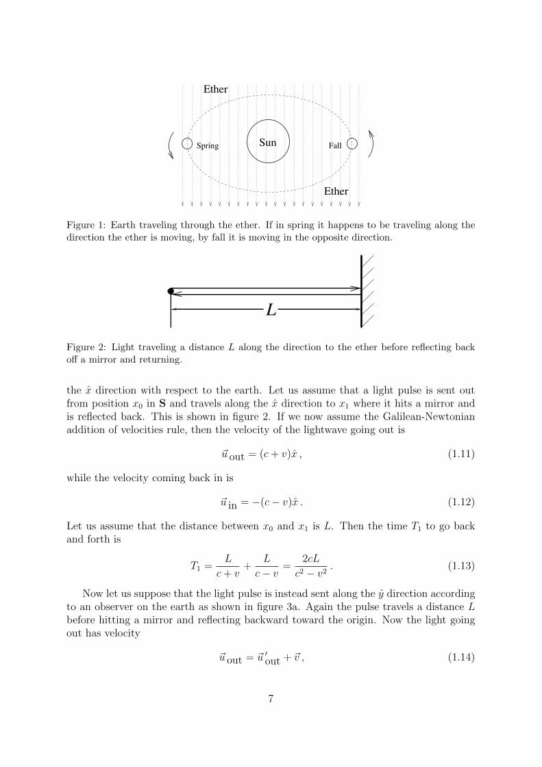
L

Figure 2: Light traveling a distance L along the direction to the ether before reflecting backoff a mirror and returning.

the x direction with respect to the earth. Let us assume that a light pulse is sent outfrom position x0 in S and travels along the x direction to x1 where it hits a mirror andis reflected back. This is shown in figure 2. If we now assume the Galilean-Newtonianaddition of velocities rule, then the velocity of the lightwave going out is

~u out = (c+ v)x , (1.11)

while the velocity coming back in is

~u in = −(c− v)x . (1.12)

Let us assume that the distance between x0 and x1 is L. Then the time T1 to go backand forth is

T1 =L

c+ v+

L

c− v=

2cL

c2 − v2. (1.13)

Now let us suppose that the light pulse is instead sent along the y direction accordingto an observer on the earth as shown in figure 3a. Again the pulse travels a distance Lbefore hitting a mirror and reflecting backward toward the origin. Now the light goingout has velocity

~u out = ~u ′out + ~v , (1.14)

7

L

avc

u’ uin in

v

u’out

b

uout

Figure 3: a) Light traveling a distance L orthogonal to the direction of the ether before reflectingback off a mirror and returning. b) Addition of velocity vectors for the outgoing light wave.c) Addition of velocity vectors for the incoming light wave.

as shown in figure 3b. Since ~v and ~uout are at right angles to each other, we find usingthe Pythagoran theorem that

~u ′out · ~u′out = ~u out · ~u out + ~v · ~v . (1.15)

Since |~u ′out| = c, we find the magnitude of ~u out is

|~u out| =√c2 − v2 . (1.16)

Examing figure 3c, it is clear that the velocity vector ~u in for the return inward, has thesame magnitude as ~u out, |~u in| = |~u out|. Hence, the total time T2, for the light wave togo to the mirror and back is

T2 =L√

c2 − v2+

L√c2 − v2

=2L√c2 − v2

. (1.17)

Comparing T2 in eq. (1.17) to T1 in eq. (1.13), we see that they are different.In 1887, the physicists Michelson and Morley measured the time difference between

T1 and T2 using an interferometer. Figure 4 shows a rough sketch of an interferometerlooking down from the top. Light of a certain wavelength λ is directed toward a half-silvered mirror, also known as a beam splitter, at an angle of 45 degrees. Half the light isreflected toward the left (upward in the diagram) and half is transmitted through. Bothbeams are reflected from mirrors and are directed back toward the half-silvered mirror.Some of the light is reflected and some is transmitted from both beams. If we considerthe light that is transmitted from the first beam and reflected from the second beam,then the two beams recombine into one beam heading toward the right (down) where thelight is observed as an interference pattern. The two beams can then interfere with each

8

Mirror

Mirror

L

L

mirrorHalf!silvered

x

Figure 4: An interferometer splits light into two beams and then recombines them. Therecombined light leads to interference patterns.

other, leading to a brighter or a dimmer beam, depending on whether the interference isconstructive or destructive.

For the sake of argument, let us suppose that the ether is at rest in the sun’s restframe. Then in the earth’s rest frame, the ether is traveling at 100,000 km/hr. Letus also suppose that in the earth’s frame, the ether is traveling in the direction of theoriginal light beam. If we assume that the distance between the half-silvered mirror andthe other mirrors is L, then the time it takes the light that is originally transmitted togo back and forth from the half-silvered mirror is T1 in eq. (1.13) and the time it takesthe beam that was originally reflected to go back and forth is T2 in eq. (1.17).

As the name implies, an interferometer measures interference and the interference isdetermined by how many wavelengths one beam differs from the other. If the differenceis a a whole number then we have constructive interference and if the difference is a halfnumber of wavelengths then there is destructive interference. Let us call this difference∆n. The number of wavelengths n that can pass by in a time T is n = c T/λ. Therefore,the difference in the number of wavelengths is

∆n =c∆T

λ=c (T1 − T2)

λ. (1.18)

Now we will make an approximation. Even though 100,000 km/hr seems like a tremen-dous rate of speed, it is quite small compared to the speed of light c. Hence, we willmake the following approximations for T1 and T2 using a Taylor expansion:

T1 =2L1 c

c2 − v2=

2L1

c (1− v2/c2)≈ 2L1

c(1 + v2/c2)

T2 =2L2√c2 − v2

=2L2

c√

1− v2/c2≈ 2L2

c(1 + 1

2v2/c2) . (1.19)

We use different lengths for the two arms, in order to incorporate interference fringes. Ifwe let L1 = L + ∆L(x) and L2 = L −∆L(x), with ∆L(x) << L and x is the position

9

where the light hits the target, then the difference in wavelengths is

∆n ≈ Lv2

λ c2+

2 ∆L(x)

λ. (1.20)

If we assume that ∆L(x) = k x where k is a constant, then ∆n is linear in x. Where itis a whole number we will have constructive interference giving a light band, and whereit is half-integer there is destructive interference giving a dark band.

The actual experiment had the interferometer floating in a puddle of mercury, allow-ing the experimenters to rotate the apparatus so that the arm that was originally pointingalong the direction of the ether could be made transverse and vice versa. Hence, undera 90 degree rotation, the difference in wavelengths is

∆n′ ≈ −Lv2

λ c2+

2 ∆L(x)

λ. (1.21)

What the experimenters then measure is how this difference changes as they rotate theinterferometer, in other words, they measure δn ≡ ∆n−∆n′

δn ≈ 2Lv2

λ c2, (1.22)

where we see that the ∆L(x) has dropped out and δn is independent of x. This meansthat the interference pattern should have a constant shift to the side as the interferometeris rotated.

One wants to make L as big as possible so that δn is as big as possible, making iteasier to measure the effect. Let us plug in some numbers to get an idea on its size. ForMichelson and Morley, L was 11 m. Using λ = 5000 A= 5× 10−7 m, c = 3× 105 km/s,and v = 100, 000 km/hr ≈ 28 km/s, we find

δn ≈ 211 m

5× 10−7 m

(28 km/s

3× 105 km/s

)2

≈ 0.4 . (1.23)

This means that the interference patternshifts over by 0.4 interference bands, asshown to the right.

The accuracy of the interferometer was good enough to measure δn as small as 0.01.And they saw no measurable effect. In other words they concluded that δn < 0.01, whichmeans that v < 13, 000 km/hr. Maybe they were unlucky and measured the earth’s speedthrough the ether when it was moving in the same direction and speed as the ether. Butthat would mean that six months later the velocity should be v ≈ 200, 000 km/hr andthey should measure δn to be 1.6. But again they found δn < 0.01. It seemed that theearth was always in the rest frame of the ether!

10

1.2 Einstein’s postulates

The Michelson-Morley experiment is a null result; the earth does not seem to have anyvelocity in the ether. But we may also understand it another way – the speed that thelight travels as measured by an observer on the earth does not depend on the earth’svelocity. But the earth in the springtime and the earth in the fall are in different referenceframes. To a very good approximation each of these frames is an inertial frame (it is notexactly inertial because of the gravitational force of the sun). In 1905, based on theseobservations, Einstein made the following two postulates

1. The laws of physics are identical in any inertial frame.

2. The speed of light in a vacuum, c, is the same in any inertial frame.

The first postulate does not sound particularly radical. Newton believed the samething. It means that if you perform any sort of experiment in an inertial frame (say alaboratory in the basement of Angstrom) and perform the same experiment in a differentinertial frame (say a spaceship heading for Alpha Centauri), the result of the experimentwill be the same.

The second postulate is the groundbreaker. We can see immediately that if we startwith an inertial frame S and do a Galilean transformation to a new reference frame S′,the new reference frame S′ is not an inertial frame. This is because the velocity of a lightwave in S′ is ~v+~c, where ~c is the velocity of the lightwave in S, and so an observer usingthe coordinates of S′ would measure a light speed different from c, violating the secondpostulate.

1.3 Lorentz transformations

If Galilean transformations do not transform us from one inertial frame to another, whatdoes? To help us find the transformation, let us define some new notation. Let us writethe space-time coordinates in an inertial frame S as

(ct, x, y, z) ≡ (x0, x1, x2, x3) (1.24)

where xi, i = 1, 2, 3 are the three spatial coordinates and x0 is the time coordinate. Wehave defined x0 with a factor of c so that x0 also has dimensions of length. We willoften write a space-time coordinate as xµ, µ = 0, 1, 2, 3, putting the time coordinate onequal footing with the three spatial coordinates. xµ is an example of a “4-vector”, a 4dimensional vector with some special properties which we will describe later. We willuse Greek letters, µ, ν, λ etc. to signify the coordinates of a 4-vector. We will use Latinletters i, j, k etc. to signify the three spatial coordinates.

Let us now assume that S′ is also an inertial frame with coordinates

(ct′, x′, y′, z′) = (x0′ , x1′ , x2′ , x3′) , (1.25)

and we will write the general space-time coordinate as xµ′. Einstein’s first postulate tells

us that the transformation between coordinates in S and those in S′ is linear. To see

11

this, suppose we have a clock in S moving with constant velocity. This means that noforces are acting on the clock since S is assumed to be an inertial frame. Let us furthersuppose that the clock gives a display of the time that it measures, which we call τ . Anobserver in S then uses xµ(τ) to be the space-time position of the clock as measured byhim when the clock display is at τ . Since the clock is moving at constant velocity, thismeans that xµ(τ) is linear in τ , from which we conclude that

d2xµ

dτ 2= 0 . (1.26)

If another observer in S′ uses his coordinates to measure the space-time position of theclock xµ

′(τ) as a function of τ , he too sees that the clock is moving with constant velocity,

and by the same argument finds that

d2xµ′

dτ 2= 0 . (1.27)

Now using the chain rule of calculus we have

dxµ′

dτ=

3∑ν=0

dxν

dτ

∂xµ′

∂xν≡ dxν

dτ

∂xµ′

∂xν(1.28)

We have introduced some new notation to save us a fair amount of writing in (1.28).Notice that the index ν appears twice, once in the numerator of a derivative and oncein the denominator. It will always be the case that when the same index appears twicein this fashion, it will be summed over. Since we know that it must be summed, wemight as drop the sum notation

∑, but the sum is still there. Let us now take one more

derivative on (1.28), again using the chain rule

d2xµ′

dτ 2= 0 =

d2xν

dτ 2

∂xµ′

∂xν+dxν

dτ

dxλ

dτ

∂2xµ′

∂xν∂xλ

= 0 +dxν

dτ

dxλ

dτ

∂2xµ′

∂xν∂xλ, (1.29)

and so we conclude that

∂2xµ′

∂xν∂xλ= 0 . (1.30)

This means that

xµ′= Λµ′

ν xν + Cµ′ , (1.31)

where Λµ′ν and Cµ′ are constants. Notice that we are still using the repeated index

notation where the index ν appears in a down position in Λµ′ν and an up position in xν ,

meaning that we are summing over ν from 0 to 3. The index µ′ appears only once, inthe up position on both sides of the equation, so it is not summed over. This means that(1.31) is really four equations, one for each value of µ′. It is more convenient to consider

12

displacements, ∆xµ where ∆xµ is the difference between two events. In this case theconstant Cµ′ drops out and we find

∆xµ′= Λµ′

ν ∆xν . (1.32)

We could also consider the possibility of differentials dxµ, which one can think of asinfinitesimal displacements. For this we have the similar relation

dxµ′= Λµ′

ν dxν . (1.33)

Let us now suppose that S′ is moving with velocity ~v = vx wrt S. If the coordinatesin S′ were related to those in S by Galilean transformations we would have

∆x′ = ∆x− v∆t, ∆y′ = ∆y, ∆z′ = ∆z . (1.34)

We want to modify these equations so that they are still linear. We should also modifythem so that when ∆x = v∆t, ∆x′ = 0. Furthermore, when ∆y = 0 we have ∆y′ = 0and when ∆z = 0, we have ∆z′ = 0. The transformations that are consistent with theseconstraints are

∆x′ = γ (∆x− v∆t), ∆y′ = γy ∆y, ∆z′ = γz ∆z . (1.35)

where γ, γy and γz are constants to be determined.Now let us consider the reverse transformation that takes us back from the S′ coordi-

nates to the S coordinates. S is moving with velocity −vx wrt S′and the transformationof the coordinates is

∆x = γ (∆x′ + v∆t′), ∆y = γy ∆y′, ∆z = γz ∆z′ , (1.36)

with the γ factors being the same as in (1.35). To show that the γ factors are the same,note that (1.35) is the true for any ∆x and ∆t. Therefore, let us define ∆x = −∆x and∆x′ = −∆x′. Clearly we have that

∆x′ = γ (∆x+ v∆t) , (1.37)

and we can think of the coordinates ∆x and ∆x′ as the x coordinates in two referenceframes S and S

′but now S

′is moving with velocity −vx wrt S, the same relation that

S has to S′. Hence, (1.36) follows.To find what γ is, suppose that we have a light ray moving in the x direction in S

and let ∆xµ refer to its displacement. By Einstein’s second postulate we must have

∆x = c∆t . (1.38)

By Einstein’s second postulate, the same light ray as seen by an observer in S′ must alsobe moving with speed c and so the displacements in the primed coordinates satisfy

∆x′ = c∆t′ . (1.39)

13

Plugging these expressions into eqs. (1.35) and (1.37), we arrive at the two linear equa-tions

c∆t′ = γ (c− v)∆t

c∆t = γ (c+ v)∆t′ . (1.40)

Hence it follows that

γ2 =c2

c2 − v2=

1

1− v2/c2⇒ γ =

1√1− v2/c2

. (1.41)

Notice that γ blows up as v approaches c. In fact, if v > c then γ is imaginary! Hence,we might expect that c is a limiting velocity for v. We will see a more physical reasonfor this when we discuss causality.

We still need to find the time coordinate in S′. Notice that (1.36) can be rewrittenas

∆t′ =1

vγ∆x− 1

v∆x′ . (1.42)

Substituting the expression for ∆x′ in (1.35) into the above leads to

∆t′ =1

vγ∆x− γ

v(∆x− v∆t) = γ∆t− γ

v(1− 1/γ2)∆x

= γ∆t− γ

v(1− (1− v2/c2))∆x

∆t′ = γ(

∆t− v

c2∆x). (1.43)

We can also easily find the reverse transformation

∆t = γ(

∆t′ +v

c2∆x′

). (1.44)

Unlike Galilean transformations, we see that the time measured between events by anobserver in S′ is not the same as the time measured between events by an observer in S.

Let us now find γy and γz. We again assume that we have a light ray, but this timeit is traveling in the y direction in S. Therefore, ∆y = c∆t. In S′ the light ray will havea component in the x direction, namely ∆x′ = γ(∆x − v∆t) = −γv∆t, since ∆x = 0.The displacement of the time coordinate in S′ is ∆t′ = γ∆t. Hence the speed of thelight ray measured by an observer in S′ is√

(∆y′)2 + (∆x′)2

∆t′=

√c2γ2

y(∆t)2 + γ2v2(∆t)2

γ∆t=

√c2γ2

y + γ2v2

γ=√c2γ2

y/γ2 + v2 .(1.45)

By the second postulate this must equal c, which then gives2 γy = 1. By a similarargument we can also argue that γz = 1.

2Actually we get c for the speed if γy = −1 as well, but this is not a valid solution since it does notsmoothly go to 1 as we take v → 0.

14

Let us now collect our results in terms of the components of Λµ′ν . Let us rewrite our

equations in the 4-vector notation:

∆x0′ = γ(

∆x0 − v

c∆x1

)∆x1′ = γ

(∆x1 − v

c∆x0

)∆x2′ = ∆x2

∆x3′ = ∆x3 . (1.46)

Comparing (1.46) with (1.32) we find that the components of Λµ′ν are

Λ0′0 = γ Λ0′

1 = −vcγ Λ0′

2 = 0 Λ0′3 = 0

Λ1′0 = −v

cγ Λ1′

1 = γ Λ1′2 = 0 Λ1′

3 = 0

Λ2′0 = 0 Λ2′

1 = 0 Λ2′2 = 1 Λ2′

3 = 0

Λ3′0 = 0 Λ3′

1 = 0 Λ3′2 = 0 Λ3′

3 = 1 . (1.47)

It is also convenient to write the transformations in matrix form∆x0′

∆x1′

∆x2′

∆x3′

=

γ −v

cγ 0 0

−vcγ γ 0 0

0 0 1 00 0 0 1

∆x0

∆x1

∆x2

∆x3

. (1.48)

Notice that the primed indices in Λµ′ν correspond to the rows of the matrix while the

unprimed indices correspond to the columns. So the entries in the first row go with the0′ index, those in the second row with 1′ etc., while the entries in the first column gowith the 0 index, those in the second column with 1 etc.

This transformation from S to S′ is an example of a boost, more specifically a boostin the x direction, and boosts are part of a set of transformations called Lorentz transfor-mations. We can combine two Lorentz transformations to give a third transformation.For example, suppose that we have a third inertial frame S′′, with coordinates related tothe coordinates in S′ by

∆xµ′′

= Λµ′′ν′∆x

ν′ , (1.49)

where Λµ′′ν′ is the Lorentz transformation relating S′′ to S′. Then these coordinates can

be related to those in S by

∆xµ′′

= Λµ′′ν′Λ

ν′λ∆x

λ = (ΛΛ)µ′′λ∆x

λ . (1.50)

Notice that the ν ′ index in Λµ′′ν′ and Λν′

λ is repeated, hence it is summed over. In termsof matrices, we can write this as

∆x0′′

∆x1′′

∆x2′′

∆x3′′

=

Λ0′′

0′ Λ0′′1′ Λ0′′

2′ Λ0′′3′

Λ1′′0′ Λ1′′

1′ Λ1′′2′ Λ1′′

3′

Λ2′′0′ Λ2′′

1′ Λ2′′2′ Λ2′′

3′

Λ3′′0′ Λ3′′

1′ Λ3′′2′ Λ3′′

3′

Λ0′0 Λ0′

1 Λ0′2 Λ0′

3

Λ1′0 Λ1′

1 Λ1′2 Λ1′

3

Λ2′0 Λ2′

1 Λ2′2 Λ2′

3

Λ3′0 Λ3′

1 Λ3′2 Λ3′

3

∆x0

∆x1

∆x2

∆x3

,(1.51)

15

where the matrices are multiplied together in the usual fashion of matrix multiplication.In particular, let us suppose that S′′=S, meaning that Λµ

ν′ = Λ−1µν′ , where Λ−1 refers

to the inverse of the matrix in (1.48). It is not hard to check that

Λ−1 =

γ +v

cγ 0 0

+vcγ γ 0 0

0 0 1 00 0 0 1

, (1.52)

which is consistent with the transformations in (1.36). In fact, let us explicitly checkthis:

γ +vcγ 0 0

+vcγ γ 0 0

0 0 1 00 0 0 1

γ −vcγ 0 0

−vcγ γ 0 0

0 0 1 00 0 0 1

=

γ2 − v2

c2γ2 −v

cγ2 + v

cγ2 0 0

+vcγ2 − v

cγ2 γ2 − v2

c2γ2 0 0

0 0 1 00 0 0 1

=

1 0 0 00 1 0 00 0 1 00 0 0 1

. (1.53)

The convention is to write Λ−1µν′ as Λµ

ν′ , that is without the “−1” exponent, since fromthe position of the primed and unprimed indices it is clear that this is the inverse of Λµ′

ν .We can also have boosts in directions other than the x direction. For example a boost

in the y direction with velocity v would look like

Λy−boost =

γ 0 −v

cγ 0

0 1 0 0−vcγ 0 γ 0

0 0 0 1

, (1.54)

which is a different Lorentz transformation. In fact we can have Lorentz transformationsthat are not boosts at all. These are rotations in the spatial directions. For example, arotation of angle φ in the x − y plane leaves the x0 and x3 coordinates alone and onlymixes the x1 and x2 coordinates. The matrix for this Lorentz transformation is given by

Λrot =

1 0 0 00 cosφ − sinφ 00 sinφ cosφ 00 0 0 1

, (1.55)

In fact, there is a way of reformulating boosts so that they look like the rotations in(1.55). We can define the rapidity, ξ, as cosh ξ = γ and sinh ξ = v

cγ, where cosh and

sinh refers to the hyperbolic cosine and hyperbolic sine respectively. Notice that thetrigonometric identity cosh2 ξ − sinh2 ξ = 1 is automatically satisfied. Then the boostmatrix Λ in (1.48) becomes

Λ =

cosh ξ − sinh ξ 0 0− sinh ξ cosh ξ 0 0

0 0 1 00 0 0 1

, (1.56)

16

with an obvious similarity to the transformation in (1.55).

1.4 Extra: Lorentz transformations form a group

This subsection is outside the main part of the course and may be skipped by those ofyou who are pressed for time or have something better to do.

Lorentz transformations make what is called the Lorentz group. Let’s define a group.A group G has the following properties.

1. A group has an operation called “multiplication”, which we denote by “·”.

2. If g and h are elements of G, then g · h is also an element of G.

3. A group has a unique element “1”, such that 1 · g = g · 1 = g.

4. Every element g has a unique inverse g−1 which is also an element of G such thatg · g−1 = g−1 · g = 1.

That’s it. Notice one statement we did not make is that g and h commute, namelyg · h = h · g. If this statement were true for all g and h in G, then we would say that thegroup is Abelian.

Let us now apply this to Lorentz transformations. The 4 × 4 matrices Λ form arepresentation of the group. There are other representations but we will not be concernedwith those here. Group multiplication is just matrix multiplication, to wit if Λ is oneelement of the group and Λ is another element of the group, then ΛΛ is another elementof the group. In general ΛΛ 6= ΛΛ. For example, a simple exercise shows that for thetransformations in (1.56) and (1.55) that ΛΛrot 6= ΛrotΛ

1.5 A relativistic invariant and proper time

An important part of this course is finding quantities that are the same for any inertialframe. Such a quantity is called a relativistic invariant, or simply an invariant. A mainreason why such quantities are useful is that they are often easy to compute in oneinertial frame, but not so easy in another one. So if we want to compute the invariant,we simply boost to the frame where it is easy to compute the invariant.

One such invariant is given by

(∆x0)2 − (∆x1)2 − (∆x2)2 − (∆x3)2 ≡ −(∆s)2 ≡ c2(∆τ)2 . (1.57)

∆s is called the invariant length and τ is the proper time. Notice that this invariantlength is similar looking to a length of a vector in 4 dimensions. The only difference isthe relative minus sign between the x0 component and the three spatial components.

17

Let’s now show that this is an invariant under Lorentz transformations. Let us assumethat we have the Lorentz boost in (1.48). Then

(∆x0′)2 − (∆x1′)2 − (∆x2′)2 − (∆x3′)2

=(γ∆x0 − v

cγ∆x1

)2

−(γ∆x1 − v

cγ∆x0

)2

− (∆x2)2 − (∆x3)2

= γ2

(1− v2

c2

)((∆x0)2 − (∆x1)2)− (∆x2)2 − (∆x3)2

= (∆x0)2 − (∆x1)2 − (∆x2)2 − (∆x3)2 . (1.58)

Hence, it is the same in both frames. It is clear that we could just as easily boost in adifferent direction and still find it invariant. A spatial rotation is also invariant since thespatial parts of (1.57) are the negative length squared of a three dimensional vector, andthis length is invariant under three-dimensional rotations.

Let us now explain the term “proper time”. Suppose that ∆xµ is the displacementvector for a body with constant velocity. If S′ is the rest-frame of the particle, thenin this frame the spatial components of the displacement are zero, since the body isnot moving in this frame. Hence, ∆τ = ∆t, so the proper time is the elapsed time asmeasured by a clock in its rest-frame.

Note that the invariant for differentials is

(dx0)2 − (dx1)2 − (dx2)2 − (dx3)2 ≡ −(ds)2 ≡ c2(dτ)2 . (1.59)

18

Px

x0

1

Figure 5: A space-time diagram with the origin labeled by event P and light-like trajectoriesshown with dashed lines.

2 Relativistic Physics

2.1 Space-time diagrams

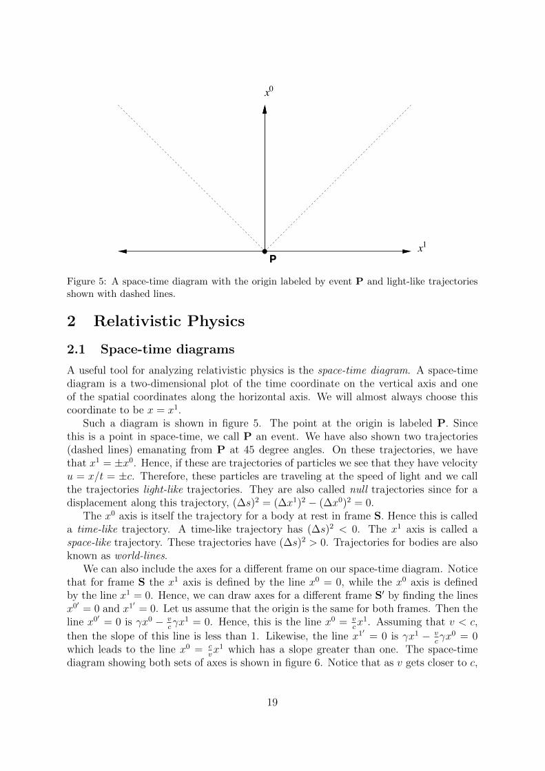
A useful tool for analyzing relativistic physics is the space-time diagram. A space-timediagram is a two-dimensional plot of the time coordinate on the vertical axis and oneof the spatial coordinates along the horizontal axis. We will almost always choose thiscoordinate to be x = x1.

Such a diagram is shown in figure 5. The point at the origin is labeled P. Sincethis is a point in space-time, we call P an event. We have also shown two trajectories(dashed lines) emanating from P at 45 degree angles. On these trajectories, we havethat x1 = ±x0. Hence, if these are trajectories of particles we see that they have velocityu = x/t = ±c. Therefore, these particles are traveling at the speed of light and we callthe trajectories light-like trajectories. They are also called null trajectories since for adisplacement along this trajectory, (∆s)2 = (∆x1)2 − (∆x0)2 = 0.

The x0 axis is itself the trajectory for a body at rest in frame S. Hence this is calleda time-like trajectory. A time-like trajectory has (∆s)2 < 0. The x1 axis is called aspace-like trajectory. These trajectories have (∆s)2 > 0. Trajectories for bodies are alsoknown as world-lines.

We can also include the axes for a different frame on our space-time diagram. Noticethat for frame S the x1 axis is defined by the line x0 = 0, while the x0 axis is definedby the line x1 = 0. Hence, we can draw axes for a different frame S′ by finding the linesx0′ = 0 and x1′ = 0. Let us assume that the origin is the same for both frames. Then theline x0′ = 0 is γx0 − v

cγx1 = 0. Hence, this is the line x0 = v

cx1. Assuming that v < c,

then the slope of this line is less than 1. Likewise, the line x1′ = 0 is γx1 − vcγx0 = 0

which leads to the line x0 = cvx1 which has a slope greater than one. The space-time

diagram showing both sets of axes is shown in figure 6. Notice that as v gets closer to c,

19

1’

0

x1P

x0’

x

x

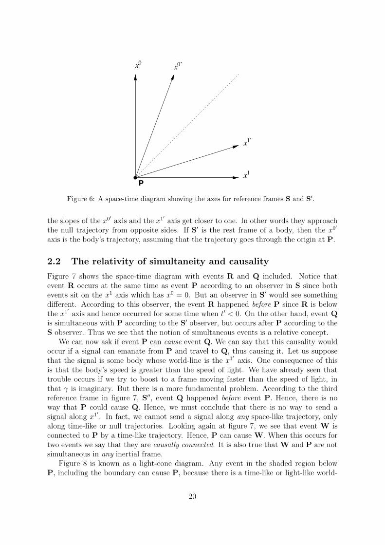
Figure 6: A space-time diagram showing the axes for reference frames S and S′.

the slopes of the x0′ axis and the x1′ axis get closer to one. In other words they approachthe null trajectory from opposite sides. If S′ is the rest frame of a body, then the x0′

axis is the body’s trajectory, assuming that the trajectory goes through the origin at P.

2.2 The relativity of simultaneity and causality

Figure 7 shows the space-time diagram with events R and Q included. Notice thatevent R occurs at the same time as event P according to an observer in S since bothevents sit on the x1 axis which has x0 = 0. But an observer in S′ would see somethingdifferent. According to this observer, the event R happened before P since R is belowthe x1′ axis and hence occurred for some time when t′ < 0. On the other hand, event Qis simultaneous with P according to the S′ observer, but occurs after P according to theS observer. Thus we see that the notion of simultaneous events is a relative concept.

We can now ask if event P can cause event Q. We can say that this causality wouldoccur if a signal can emanate from P and travel to Q, thus causing it. Let us supposethat the signal is some body whose world-line is the x1′ axis. One consequence of thisis that the body’s speed is greater than the speed of light. We have already seen thattrouble occurs if we try to boost to a frame moving faster than the speed of light, inthat γ is imaginary. But there is a more fundamental problem. According to the thirdreference frame in figure 7, S′′, event Q happened before event P. Hence, there is noway that P could cause Q. Hence, we must conclude that there is no way to send asignal along x1′ . In fact, we cannot send a signal along any space-like trajectory, onlyalong time-like or null trajectories. Looking again at figure 7, we see that event W isconnected to P by a time-like trajectory. Hence, P can cause W. When this occurs fortwo events we say that they are causally connected. It is also true that W and P are notsimultaneous in any inertial frame.

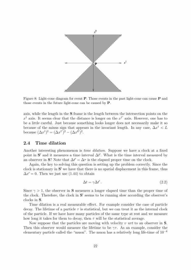
Figure 8 is known as a light-cone diagram. Any event in the shaded region belowP, including the boundary can cause P, because there is a time-like or light-like world-

20

W

0

x1

x1’’

P

x0’

x1’

R

Q

x0’’x

Figure 7: Event R is simultaneous with P according to an observer in S but not accordingto an observer in S′. Similarly, event Q is simultaneous with event P according to an observerin S′, but not according to an observer in S. Event W is causally connected to P.

line that connects this event to P. This region is called the past light-cone. Similarly,any event in shaded region above P can be caused by P because there is a time-like orlight-like world-line connecting P to the event.

2.3 Length contraction

Suppose we have a bar of length L that is stationary in S′ and is aligned along the xaxis. What length would an observer in S measure?

In problems of this type, the key to solving this question is properly setting up theequations. Firstly, how would an observer in S make the measurement? A reasonablething to do is to measure the positions of the front and back of the bar simultaneously,that is find their positions at the same time t, and then measure the displacement, ∆x.Since the observer is making a simultaneous measurement according to his clocks, wehave that ∆t = 0. We also know that the displacement in S′ is ∆x′ = L since the bar isstationary in this frame.

We now use the relations in (1.36) and (1.44) to write

∆t = 0 = γ(

∆t′ +v

c2∆x′

)⇒ ∆t′ = − v

c2∆x′

∆x = γ (∆x′ + v∆t′) = γ

(1− v2

c2

)∆x′ =

L

γ. (2.1)

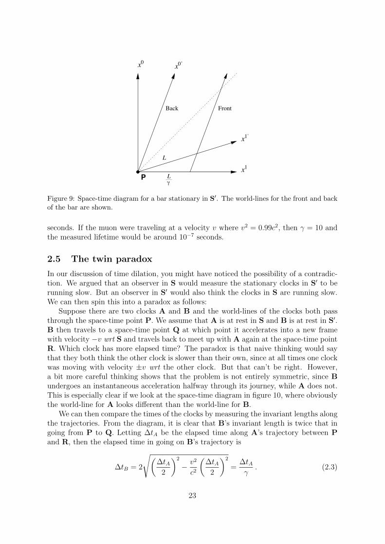
Hence the observer in S measures a contracted length since γ > 1.This is particularly clear if we look at the corresponding space-time diagram shown

in figure 9. In this diagram we have shown the trajectories for the front and back ofthe bar. We are still assuming that S′ is the rest-frame. The length of the bar in therest-frame is the length between the intersection points of the trajectories with the x1′

21

P

0

x1

x

Figure 8: Light-cone diagram for event P. Those events in the past light-cone can cause P andthose events in the future light-cone can be caused by P.

axis, while the length in the S frame is the length between the intersection points on thex1 axis. It seems clear that the distance is longer on the x1′ axis. However, one has tobe a little careful. Just because something looks longer does not necessarily make it sobecause of the minus sign that appears in the invariant length. In any case, ∆x1 < Lbecause (∆x1)2 = (∆x1′)2 − (∆x0′)2.

2.4 Time dilation

Another interesting phenomenon is time dilation. Suppose we have a clock at a fixedpoint in S′ and it measures a time interval ∆t′. What is the time interval measured byan observer in S? Note that ∆t′ = ∆τ is the elapsed proper time on the clock.

Again, the key to solving this question is setting up the problem correctly. Since theclock is stationary in S′ we have that there is no spatial displacement in this frame, thus∆x′ = 0. Then we just use (1.44) to obtain

∆t = γ∆t′ . (2.2)

Since γ > 1, the observer in S measures a longer elapsed time than the proper time ofthe clock. Therefore, the clock in S′ seems to be running slow according the observer’sclocks in S.

Time dilation is a real measurable effect. For example consider the case of particledecay. The lifetime of a particle τ is statistical, but we can treat it as the internal clockof the particle. If we have have many particles of the same type at rest and we measurehow long it takes for them to decay, then τ will be the statistical average.

Now suppose that the particles are moving with velocity v wrt to an observer in S.Then this observer would measure the lifetime to be γτ . As an example, consider theelementary particle called the “muon”. The muon has a relatively long life-time of 10−8

22

!

0

x1P

x0’

x1’

Back Front

L

L

x

Figure 9: Space-time diagram for a bar stationary in S′. The world-lines for the front and backof the bar are shown.

seconds. If the muon were traveling at a velocity v where v2 = 0.99c2, then γ = 10 andthe measured lifetime would be around 10−7 seconds.

2.5 The twin paradox

In our discussion of time dilation, you might have noticed the possibility of a contradic-tion. We argued that an observer in S would measure the stationary clocks in S′ to berunning slow. But an observer in S′ would also think the clocks in S are running slow.We can then spin this into a paradox as follows:

Suppose there are two clocks A and B and the world-lines of the clocks both passthrough the space-time point P. We assume that A is at rest in S and B is at rest in S′.B then travels to a space-time point Q at which point it accelerates into a new framewith velocity −v wrt S and travels back to meet up with A again at the space-time pointR. Which clock has more elapsed time? The paradox is that naive thinking would saythat they both think the other clock is slower than their own, since at all times one clockwas moving with velocity ±v wrt the other clock. But that can’t be right. However,a bit more careful thinking shows that the problem is not entirely symmetric, since Bundergoes an instantaneous acceleration halfway through its journey, while A does not.This is especially clear if we look at the space-time diagram in figure 10, where obviouslythe world-line for A looks different than the world-line for B.

We can then compare the times of the clocks by measuring the invariant lengths alongthe trajectories. From the diagram, it is clear that B’s invariant length is twice that ingoing from P to Q. Letting ∆tA be the elapsed time along A’s trajectory between Pand R, then the elapsed time in going on B’s trajectory is

∆tB = 2

√(∆tA

2

)2

− v2

c2

(∆tA

2

)2

=∆tAγ

. (2.3)

23

!

0

x1P

x0’

x1’

"

!

Q

Rx

Figure 10: Space-time diagram for two clocks A and B. B has an instaneous acceleration atpoint Q.

Hence, B’s clock has less elapsed time and both sides would agree. Thus, there is noparadox.

Notice that while B’s trajectory looks longer in the diagram, the elapsed time isshorter. This is because of the relative minus sign that appears in the invariant in(1.57).

We can also obtain our result another way. Suppose that the distance that B travelsaway from A is L according to an observer in S. Then A would think the total time forB’s journey is ∆tA = 2vL. But B would see this length contracted to L/γ, so accordingto his clock the time for the journey is ∆tB = 2vL/γ = ∆tA/γ.

2.6 Velocity transformations

Suppose that a body is moving with velocity ~u ′ in inertial frame S′. What is the ve-locity ~u measured by an observer in S? To measure a velocity, one measures the spatialdisplacement and divides by the elapsed time. Thus, the velocity components in S′ aregiven by

u′x =∆x′

∆t′, u′y =

∆y′

∆t′, u′z =

∆z′

∆t′, (2.4)

while the components in S are

ux =∆x

∆t, uy =

∆y

∆t, uz =

∆z

∆t, (2.5)

24

We again make use of the transformations in (1.36) and (1.44) to write the velocitycomponents in (2.5) as

ux =∆x′ + v∆t′

∆t′ + vc2

∆x′=

u′x + v

1 + u′xvc2

,

uy =∆y′

γ(∆t′ + vc2

∆x′)=

u′y

γ(1 + u′xvc2

),

uz =∆z′

γ(∆t′ + vc2

∆x′)=

u′z

γ(1 + u′xvc2

). (2.6)

Notice that these components do not satisfy ~u = ~u ′+~v, in other words, the Galileanaddition of velocities is no longer true. However, for very small velocities, where |~u| << c

and v << c, we have that u′xvc2

<< 1. Thus the denominators in (2.6) are very close to 1,and so addition of velocities is approximately true.

We can also show that if |~u ′| < c and v < c, then |~u| < c. To see this, consider thecombination

c2 − (~u ′)2 =c2(∆t′)2 − (∆x′)2 − (∆y′)2 − (∆z′)2

(∆t′)2> 0 . (2.7)

The numerator is the invariant in (1.57) and since (∆t′)2 > 0, the numerator must alsobe greater than zero. Therefore

c2 − (~u)2 =c2(∆t)2 − (∆x)2 − (∆y)2 − (∆z)2

(∆t)2> 0 . (2.8)

2.7 Acceleration

Let us now consider the case of acceleration and how an observer in a frame differentfrom the accelerating object would see this. The proper acceleration, ~α is defined asthe acceleration in the rest frame of the accelerated body. Now since this rest frameis accelerating with respect to the observer’s rest frame, which we are assuming is aninertial frame, it means that the body’s rest frame is not an inertial frame. However, atany time there is an inertial frame where the body is at rest. We call this inertial frameits instantaneous rest frame. This can also be called the momentary rest frame. At alater time, the instantaneous inertial frame is different from the one it is in now.

To avoid too many complications, let us simplify the problem a bit and assume thatthe velocities and accelerations are in the x direction only, so ~α = αx. We then let S bethe frame of the observer and S′(t) be the instantaneous rest frame at time t. If ~u = u xis the velocity of the body as seen by the observer, then v = u at t. In S′(t) we havethat u′ = 0. At a slightly later time t + dt, where dt is assumed to be an infinitesimaldisplacement, we have that u′ has an infinitesimal change, du′, since S′(t) is no longer theinstantaneous rest frame, S′(t+dt) is. But from the definition of the proper acceleration,we have that

du′ = α dt′ . (2.9)

25

Since S′(t) is the instantaneous rest frame, dt is related to dt′ by time dilation:

dt = γu dt′ , γu =

1√1− u2

c2

. (2.10)

The change in velocity du as seen by the observer in S is then found using the velocitytransformation in (2.6). Given the velocity in S′(t) is du′ and the velocity in S is u+ duthen the transformation formula leads to

du =du′ + u

1 + u du′

c2

− u ≈ (du′ + u)

(1− u du′

c2

)− u ≈ du′

(1− u2

c2

), (2.11)

where we used that |u| < c and |du′| << c to justify the approximations.The acceleration, a, as measured by the observer in S is then

a =du

dt=du′

dt′

(1− u2

c2

)3/2

=α

γu3. (2.12)

Notice that a is approaching 0 as u approaches c, which is reasonable since we shouldnot be able to accelerate the body through the speed of light.

Let us take the further special case that the proper acceleration α is constant. Wethen observe that

d

dt(γu u) = γu

du

dt+ u

d

dt

1√1− u2

c2

=

(γu +

u2

c2γu

3

)du

dt= γu

3 du

dt. (2.13)

Hence, we can write (2.12) as

d

dt(γu u) = α (2.14)

which has the solution

γu u = αt+ u0 (2.15)

where u0 is a constant. If we take the initial condition that u = 0 at t = 0, then u0 = 0.Squaring both sides of the above equation gives

u2

1− u2

c2

= α2t2 , (2.16)

which has the solution

u =αt√

1 + α2t2/c2. (2.17)

Now using u = dxdt

we get

dx =αt dt√

1 + α2t2/c2, (2.18)

26

Figure 11: Graph of the hyperbolic trajectory in (2.20). The horizontal axis is the x coordinateand the vertical axis is the x0 = ct coordinate. The dashed lines are light-like lines that definethe limits of the hyperbola. The hyperbola intersects the x-axis at x = c2/α.

which can be integrated to give

x =c2

α

√1 +

α2t2

c2+ x0 , (2.19)

where x0 is a constant. Since the constant is just a shift in x we drop it. Hence, thissolution can be written as

x2 − (ct)2 =c4

α2, (2.20)

which is the equation for a hyperbola. This solution is graphed in figure 11, where thehorizontal axis is the x axis and the vertical axis is the x0 = ct axis. The hyperbolacrosses the x axis at x = c2/α. Notice that as t becomes large, the hyperbola approachesthe light-like trajectory which is the dashed line in the plot. Interestingly, if at t = 0 alight ray is emitted at x = 0, we see that it will never catch up with the acceleratingbody since the dashed line never intersects the hyperbola.

2.8 Doppler shifts

If you are standing at a railroad crossing and an approaching train blows its whistle, thewhistle will suddenly drop in pitch as the train passes. This phenomenon is due to theDoppler shift of the train’s sound waves. When the train is moving toward us, the pitchis shifted upward, but when it is moving away it is shifted downward. We can then askwhat will happen to lightwaves of wavelength λ, which is related to the frequency ν byλ = c/ν.

Suppose we have a light source whose rest-frame is S′ and is shining light at anobserver in S. We can think of the light source as a clock which is sending a signal at

27

a regular time interval, ∆t′ = 1/ν. In other words, this is the time for one wavelengthof light to be emitted. The signal travels at the speed of light, c. This clock is timedilated in S to ∆t = γ∆t′. But the question is more involved that just time dilation.The light being emitted is being observed by an observer at a fixed position in S. Weare not comparing the clock in S′ with a series of clocks it passes in S as the light sourcemoves along.

Let us say that at t = 0 the light source is at x = 0 moving with velocity v in the xdirection. The observer is fixed at x = 0. If the light source sends a signal at t = 0 thenthe observer receives it instantaneously because the signal has zero distance to travel.The source then sends another signal at time t = ∆t. But the light source is movingaway from the observer and this signal is sent from position x = v∆t, and so the observerdoes not receive it immediately, but at a later time

t = ∆T = ∆t+v∆t

c= γ∆t′

(1 +

v

c

)= ∆t′

√1 + v/c

1− v/c. (2.21)

Hence the time it takes the observer to see one wavelength is ∆T and so the lightfrequency as seen by the observer is

νobs =1

∆T= ν

√1− v/c1 + v/c

= ν

√c− vc+ v

, (2.22)

and the wavelength is

λobs =c

νobs

= λ

√c+ v

c− v. (2.23)

Since the wavelength increases, we call this a red-shift.To find the shift if the source is moving toward the observer, all we need to do is

replace v with −v, hence we have

λobs = λ

√c− vc+ v

. (2.24)

Since the wavelength is smaller, we call this a blue-shift.It is instructive to look at the space-time diagram for this process. Figure 12 shows

the world-line of the source as the x0′ axis. Included are the world-lines for light signalssent a time ∆t′ apart according to the source’s clock and sent back toward the observerat x = 0. The diagram shows the difference between ∆t and ∆T .

We can also generalize this to include a light source that is not moving directly awayor toward the observer, but at an angle θ, as shown in figure 13. In this case, during thetime interval ∆t the source has moved a distance v cos θ∆t away from the observer, sowe have that ∆T is

∆T = ∆t+v cos θ∆t

c= γ∆t′

(1 +

v cos θ

c

), (2.25)

28

T

0

x1

x0’

x1’

!c

!c

Source

Observer t

x

Figure 12: A space-time diagram for a light source emitting light toward an observer. Thesource’s world-line is the x0′ axis, while the observer’s world-line is the x0 axis.

and so the frequency and wavelength seen by the observer is

νobs =1

∆T= ν

√1− v2/c2

1 + vc

cos θ

λobs = λ1 + v

ccos θ√

1− v2/c2. (2.26)

2.9 A little cosmology

Our universe is expanding. How do we know this? We can see distant galaxies beingredshifted. The further away the galaxy the bigger the redshift. To describe the redshift,cosmologists define a quantity Z, given by

Z ≡ λobs

λgalaxy

− 1 , (2.27)

where λgalaxy is the wavelength in the rest frame of the galaxy and λobs is the galaxy’swavelength as measured by an observer on earth. If the galaxy is redshifted, then Z > 0.Using the result for the redshift in (2.23), we have

Z =

√c+ v

c− v− 1 . (2.28)

We can then invert this equation to find the receding velocity of the galaxy given thevalue of Z:

c+ v

c− v= (Z + 1)2 ⇒ v =

Z(2 + Z)

2 + Z(2 + Z)c . (2.29)

29

!

Source

Observer

Figure 13: A light source moving away from an observer at an angle θ.

It has been observed that the the further away the galaxy, the faster it is receding.In fact the relation between the velocity and the distance is very close to linear, givenby

v = H0D , (2.30)

where D is the distance and H0 is a constant called the Hubble constant. It turns out thatit is much easier to measure v than D. But over the last ten or fifteen years, an effectiveway to measure D was found by not observing galaxies, but supernovae. A supernova isan exploding star and those of a certain type were found to have very uniform properties.So the brightness of the supernova during the course of its explosion (which could beobserved for several weeks) could be used to judge its distance.

At present, the farthest away supernova had Z = 1.7, which translates into a velocityof v = 0.76 c. The present value for H0 is approximately H0 ≈ 70 km/s-Mpsc. Mpscstands for Megaparsec which equals 3.26 × 106 light years, where a light year is thedistance light travels in one year. Hence, the distance of this far away supernova is

D =v

H0

=(0.76)(3× 105 km/s)

70 km/s× 3.26× 106 light years

= 10.6× 109 light years . (2.31)

This can be compared to the size of the visible universe which is 13.7× 109 light years.Hence, this supernova was a significant distance away compared to the overall size of thevisible universe.

30

2.10 The drag effect

An interesting phenomenon was known to 19th century physicists. They had observedthat in a liquid moving with velocity v along the x direction, the speed of light alongthe same direction is

u = u′ + kv , (2.32)

where u′ is the velocity when the fluid is at rest and

k = 1− 1

n2, (2.33)

where n is the index of refraction. Hence by definition, u′ = c/n. In the middle of thecentury Fresnel came up with an ether based explanation for why this should happen,basically arguing that the fluid pushed the ether along with it.

But we can explain this using velocity transformations. We let S′ be the rest frame ofthe liquid and S be the rest frame of the observer measuring the light’s speed. We thenassume that v << c, since afterall, we don’t expect any liquids to be traveling anywherenear the speed of light. Using (2.6) and Taylor expanding to first order in v we have

u =u′ + v

1 + u′v/c2≈ (u′ + v)

(1− u′v

c2

)≈ u′ + v − u′2v

c2= u′ + v

(1− 1

n2

), (2.34)

which is the result we are looking for. Incidentally, notice that the speed of the light isnot the same in different reference frames. But this does not contradict Einstein’s secondpostulate because the light is not traveling in a vacuum.

2.11 Aberration

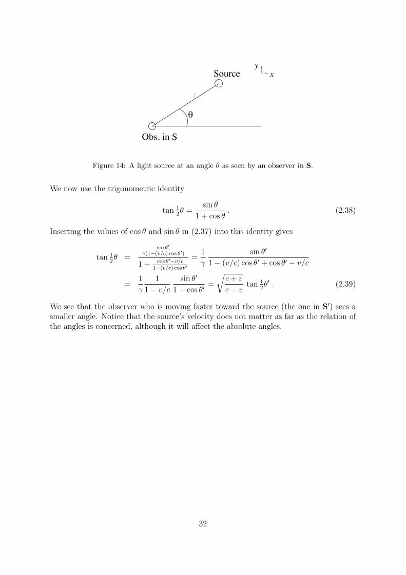
Aberration is the effect that observers in different inertial frames can measure differentangles for a light source. For this problem we can restrict the spatial dimensions to thex and y coordinates. We again assume that the two observers are in different frames Sand S′, and that S′ is moving with velocity ~v = vx wrt S′. An observer at the spatialorigin of S sees a light source at an angle θ away from the x-axis. Figure 14 shows adiagram of this. The observer in S′ sees the same light source at a different angle θ′.The problem is to relate the two angles.

Again we can use the velocity transformations in (2.6) to find the relation. Fromfigure 14 we see that the velocity components of the light coming from the source as seenby the observer in S are

ux = −c cos θ uy = −c sin θ , (2.35)

while those seen by the observer in S′ are

u′x = −c cos θ′ u′y = −c sin θ′ . (2.36)

Substituting these expressions into (2.6) we find

− cos θ =− cos θ′ + v/c

1− (v/c) cos θ′, − sin θ =

− sin θ′

γ(1− (v/c) cos θ′). (2.37)

31

y

!

Source

Obs. in S

x

Figure 14: A light source at an angle θ as seen by an observer in S.

We now use the trigonometric identity

tan 12θ =

sin θ

1 + cos θ. (2.38)

Inserting the values of cos θ and sin θ in (2.37) into this identity gives

tan 12θ =

sin θ′

γ(1−(v/c) cos θ′)

1 + cos θ′−v/c1−(v/c) cos θ′

=1

γ

sin θ′

1− (v/c) cos θ′ + cos θ′ − v/c

=1

γ

1

1− v/csin θ′

1 + cos θ′=

√c+ v

c− vtan 1

2θ′ . (2.39)

We see that the observer who is moving faster toward the source (the one in S′) sees asmaller angle. Notice that the source’s velocity does not matter as far as the relation ofthe angles is concerned, although it will affect the absolute angles.

32

3 Tensors

Tensors are very useful because they have nice transformation properties under Lorentztransformations3. So if physical quantities can be written in terms of tensors, then weknow how to find these quantities in different inertial frames. In fact, we can evengeneralize this to transformations from any frame (not necessarily an inertial frame) toany other frame, but we won’t worry about that here. So if we can put physical quantitiesinto tensor form, then we have a recipe for finding these quantities in any inertial frame.

Tensors can come with two types of indices. These are “upper” indices and “lower”indices. The distinction between the two is important because the two types of indicestransform differently under Lorentz transformations.

Let us start with one of the simplest tensors which is one we have already introduced,the displacement “4-vector” ∆xµ. Since this has an upper index, we say that this is acontravariant vector. The upper index µ refers to one of 4 possible values 0, 1, 2 or 3. The0 component is the component along the time direction. The other three componentsare called spatial components. The 4 components of ∆xµ can now be written as

∆xµ : (∆x0,∆x1,∆x2,∆x3) = (c∆t,∆x,∆y,∆z) . (3.1)

Notice the first coefficient when written with ∆t has a factor of c so that the ∆x0 has unitsof length, just like the spatial components. We also sometimes write ∆xµ : (∆x0,∆~x).Lower case Greek letters are used for space-time indices, while lower case Roman letters(i, j, k etc.) are used for spatial indices only. The indices are associated with a particularinertial frame S, and the variables xµ are known as the coordinates of that frame.

Now that we have a tensor, in this case a contravariant vector, let us transform it toa new frame. Suppose we start with the 4-vector Aµ in frame S. The goal is to find the4-vector in the new frame S′. This is done through a Lorentz transformation. There are 6independent transformations. Three of these are the boosts along the three independentspatial directions. The boost is completely determined by the relative velocity ~v that S′

is moving with respect to (wrt) S. The other 3 independent transformations are spatialrotations. A rotation takes place in a plane, so the independent transformations are the3 ways of choosing 2 spatial directions, (x, y), (y, z) and (z, x). Along with the plane,we should also specify the angle through which we rotate. In any case, any Lorentztransformation can be made with some combination of these types of transformations.

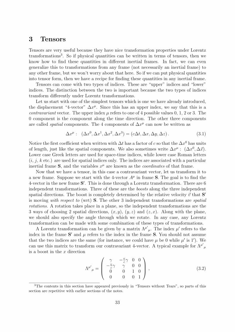
A Lorentz transformation can be given by a matrix Λµ′µ. The index µ′ refers to the

index in the frame S′ and µ refers to the index in the frame S. You should not assumethat the two indices are the same (for instance, we could have µ be 0 while µ′ is 1′). Wecan use this matrix to transform our contravariant 4-vector. A typical example for Λµ′

µ

is a boost in the x direction

Λµ′µ =

γ −v

cγ 0 0

−vcγ γ 0 0

0 0 1 00 0 0 1

, (3.2)

3The contents in this section have appeared previously in “Tensors without Tears”, so parts of thissection are repetitive with earlier sections of the notes.

33

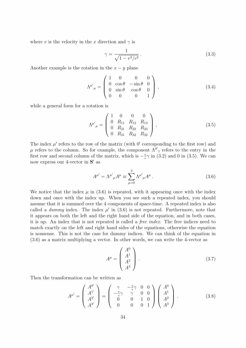
where v is the velocity in the x direction and γ is

γ =1√

1− v2/c2. (3.3)

Another example is the rotation in the x− y plane

Λµ′µ =

1 0 0 00 cos θ − sin θ 00 sin θ cos θ 00 0 0 1

, (3.4)

while a general form for a rotation is

Λµ′µ =

1 0 0 00 R11 R12 R13

0 R21 R22 R23

0 R31 R32 R32

, (3.5)

The index µ′ refers to the row of the matrix (with 0′ corresponding to the first row) andµ refers to the column. So for example, the component Λ0′

1 refers to the entry in thefirst row and second column of the matrix, which is −v

cγ in (3.2) and 0 in (3.5). We can

now express our 4-vector in S′ as

Aµ′= Λµ′

µAµ ≡

3∑µ=0

Λµ′µA

µ . (3.6)

We notice that the index µ in (3.6) is repeated, with it appearing once with the indexdown and once with the index up. When you see such a repeated index, you shouldassume that it is summed over the 4 components of space-time. A repeated index is alsocalled a dummy index. The index µ′ in (3.6) is not repeated. Furthermore, note thatit appears on both the left and the right hand side of the equation, and in both cases,it is up. An index that is not repeated is called a free index. The free indices need tomatch exactly on the left and right hand sides of the equations, otherwise the equationis nonsense. This is not the case for dummy indices. We can think of the equation in(3.6) as a matrix multiplying a vector. In other words, we can write the 4-vector as

Aµ =

A0

A1

A2

A3

. (3.7)

Then the transformation can be written as

Aµ′=

A0′

A1′

A2′

A3′

=

γ −v

cγ 0 0

−vcγ γ 0 0

0 0 1 00 0 0 1

A0

A1

A2

A3

. (3.8)

34

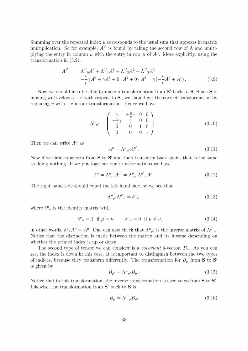
Summing over the repeated index µ corresponds to the usual sum that appears in matrixmultiplication. So for example, A1′ is found by taking the second row of Λ and multi-plying the entry in column µ with the entry in row µ of Aµ. More explicitly, using thetransformation in (3.2),

A1′ = Λ1′0A

0 + Λ1′1A

1 + Λ1′2A

2 + Λ1′3A

3

= −vcγA0 + γA1 + 0 · A2 + 0 · A3 = γ(−v

cA0 + A1) . (3.9)

Now we should also be able to make a transformation from S′ back to S. Since S ismoving with velocity −v with respect to S′, we should get the correct transformation byreplacing v with −v in our transformation. Hence we have

Λµµ′ =

γ +v

cγ 0 0

+vcγ γ 0 0

0 0 1 00 0 0 1

. (3.10)

Then we can write Aµ asAµ = Λµ

µ′Aµ′ . (3.11)

Now if we first transform from S to S′ and then transform back again, that is the sameas doing nothing. If we put together our transformations we have

Aµ = Λµµ′A

µ′ = Λµµ′Λ

µ′νA

ν . (3.12)

The right hand side should equal the left hand side, so we see that

Λµµ′Λ

µ′ν = δµν , (3.13)

where δµν is the identity matrix with

δµν = 1 if µ = ν, δµν = 0 if µ 6= ν, (3.14)

in other words, δµνAν = Aµ. One can also check that Λµ

µ′ is the inverse matrix of Λµ′µ.

Notice that the distinction is made between the matrix and its inverse depending onwhether the primed index is up or down.

The second type of tensor we can consider is a covariant 4-vector, Bµ. As you cansee, the index is down in this case. It is important to distinguish between the two typesof indices, because they transform differently. The transformation for Bµ from S to S′

is given byBµ′ = Λµ

µ′Bµ , (3.15)

Notice that in this transformation, the inverse transformation is used to go from S to S′.Likewise, the transformation from S′ back to S is

Bµ = Λµ′µBµ′ (3.16)

35

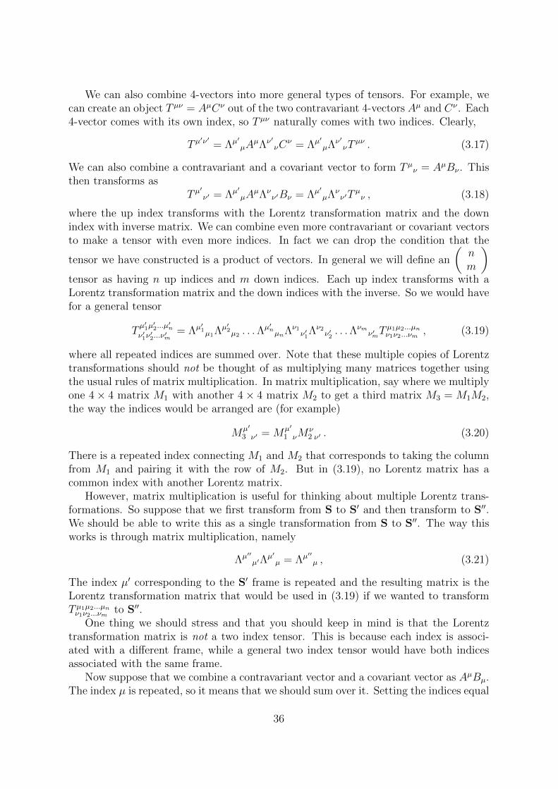
We can also combine 4-vectors into more general types of tensors. For example, wecan create an object T µν = AµCν out of the two contravariant 4-vectors Aµ and Cν . Each4-vector comes with its own index, so T µν naturally comes with two indices. Clearly,

T µ′ν′ = Λµ′

µAµΛν′

νCν = Λµ′

µΛν′νT

µν . (3.17)

We can also combine a contravariant and a covariant vector to form T µν = AµBν . Thisthen transforms as

T µ′ν′ = Λµ′

µAµΛν

ν′Bν = Λµ′µΛν

ν′Tµν , (3.18)

where the up index transforms with the Lorentz transformation matrix and the downindex with inverse matrix. We can combine even more contravariant or covariant vectorsto make a tensor with even more indices. In fact we can drop the condition that the

tensor we have constructed is a product of vectors. In general we will define an

(nm

)tensor as having n up indices and m down indices. Each up index transforms with aLorentz transformation matrix and the down indices with the inverse. So we would havefor a general tensor

Tµ′1µ

′2...µ

′n

ν′1ν′2...ν

′m

= Λµ′1µ1Λ

µ′2µ2 . . .Λ

µ′nµnΛν1

ν′1Λν2

ν′2. . .Λνm

ν′mTµ1µ2...µnν1ν2...νm

, (3.19)

where all repeated indices are summed over. Note that these multiple copies of Lorentztransformations should not be thought of as multiplying many matrices together usingthe usual rules of matrix multiplication. In matrix multiplication, say where we multiplyone 4× 4 matrix M1 with another 4× 4 matrix M2 to get a third matrix M3 = M1M2,the way the indices would be arranged are (for example)

Mµ′

3 ν′ = Mµ′

1 νMν2 ν′ . (3.20)

There is a repeated index connecting M1 and M2 that corresponds to taking the columnfrom M1 and pairing it with the row of M2. But in (3.19), no Lorentz matrix has acommon index with another Lorentz matrix.

However, matrix multiplication is useful for thinking about multiple Lorentz trans-formations. So suppose that we first transform from S to S′ and then transform to S′′.We should be able to write this as a single transformation from S to S′′. The way thisworks is through matrix multiplication, namely

Λµ′′µ′Λ

µ′µ = Λµ′′

µ , (3.21)

The index µ′ corresponding to the S′ frame is repeated and the resulting matrix is theLorentz transformation matrix that would be used in (3.19) if we wanted to transformT µ1µ2...µnν1ν2...νm

to S′′.One thing we should stress and that you should keep in mind is that the Lorentz

transformation matrix is not a two index tensor. This is because each index is associ-ated with a different frame, while a general two index tensor would have both indicesassociated with the same frame.

Now suppose that we combine a contravariant vector and a covariant vector as AµBµ.The index µ is repeated, so it means that we should sum over it. Setting the indices equal

36

like this is called contracting an index. Let us now see what this quantity is in S′. Whenwe have more than one index, each one is transformed with a Lorentz transformationmatrix. Given these transformation properties, we find

Aµ′Bµ′ = Λµ′

νAνΛµ

µ′Bµ = Λµµ′Λ

µ′νA

νBµ . (3.22)

In this last step we just rearranged the order of the terms in the equation. These arejust numbers so we are allowed to do this. Now the Λµ

µ′Λµ′ν is precisely what appears

in (3.13), so we can replace it by δµν , so we find

Aµ′Bµ′ = δµνA

νBµ = AµBµ . (3.23)

Observe that δµν is nonzero only when µ is the same as ν, and in this case it equals 1.Hence summing over ν will end up replacing the ν in Aν with a µ. However, since bothν and µ are dummy indices, we could have equally replaced µ with ν. So you can seethat you are free to relabel the dummy indices in which they appear. In other words

AµBµ = AνBν . (3.24)

We can see from the equation in (3.23) that the quantity AµBµ does not change whenyou transform to another frame.

A quantity that does not change under Lorentz transformations is known as a Lorentzinvariant, or a Lorentz scalar or sometimes just invariant or scalar. The multiplicationof two 4-vectors to make a Lorentz scalar is called a scalar product, or also inner product.This expression has no free indices, so it is like having a tensor T with no indices.According to the rules in (3.19), we would have the equation T ′ = T where the left handside refers to the tensor in S′. In other words, it is an invariant.

An important tensor is the two index tensor ηµν . This is defined as4

ηµν =

+1 0 0 00 −1 0 00 0 −1 00 0 0 −1

µν

. (3.25)

We can also write this as ηµν = diag(+1,−1,−1,−1)µν . Under the Lorentz transforma-tion

ηµ′ν′ = Λµµ′Λ

νν′ηµν = ΛT

µ′µηµνΛ

νν′ , (3.26)

where we define ΛTµ′µ ≡ Λµ

µ′ . In the last step in (3.26) we have arranged the indices sothat it has the form of multiplying 3 matrices together. By rewriting the first Lorentztransformation this way we are transposing the rows and the columns, but are otherwisedoing nothing else. If Λµ′

µ is the general rotation in (3.5) then the matrix equation in(3.26) becomes

ΛTµ′µηµνΛ

νν′ =

(ΛTηΛ

)µ′ν′

=(ηΛTΛ

)µ′ν′

, (3.27)

4Rindler uses the symbol g instead of η.

37

where ΛT is the transpose of Λ. Now for a rotation, it turns out that ΛT = Λ−1.Therefore, we have for rotations

ηµ′ν′ =

+1 0 0 00 −1 0 00 0 −1 00 0 0 −1

µ′ν′

. (3.28)

If Λµ′µ corresponds to the boost in (3.2), then ΛT = Λ and we find

ηµ′ν′ =

γ −v

cγ 0 0

−vcγ γ 0 0

0 0 1 00 0 0 1

+1 0 0 00 −1 0 00 0 −1 00 0 0 −1

γ −vcγ 0 0

−vcγ γ 0 0

0 0 1 00 0 0 1

=

γ −v

cγ 0 0

−vcγ γ 0 0

0 0 1 00 0 0 1

γ −vcγ 0 0

+vcγ −γ 0 0

0 0 −1 00 0 0 −1

=

γ2(

1− v2

c2

)0 0 0

0 −γ2(

1− v2

c2

)0 0

0 0 −1 00 0 0 −1

=

+1 0 0 00 −1 0 00 0 −1 00 0 0 −1

µ′ν′

(3.29)

We would get the same result if we were to boost in any other direction because ofthe rotational symmetry of ηµν . Therefore, ηµ′ν′ has the same form as ηµν . But it isimportant to note that ηµν is not a Lorentz invariant. This is because its indices changedunder the transformation.

We can use the η-tensor to change contravariant indices to covariant indices. So forexample consider the transformation of Aµηµν

Aµ′ηµ′ν′ = Λµ′

µAµΛλ

µ′Λνν′ηλν = Λν

ν′Λλµ′Λ

µ′µA

µηλν

= Λνν′δ

λµA

µηλν = Λνν′A

µηµν . (3.30)

Hence Aµηµν transforms as if there is only the down index ν. Therefore, we can definea covariant 4-vector from a contravariant vector by Aν ≡ Aµηµν . This process is knownas lowering an index. We can also consider the inverse of ηµν with two raised indices,such that ηµληλν = δµν . But we can also think of this as ηµν (in other words, ηµν = δµν)where the η-tensor with the down indices lowered one of the indices of ηµν . We can thenuse ηµν to raise indices; Aµ = ηµνAν . Obviously, this is called raising an index. We

38

can raise or lower several indices by using more than one η-tensor. If we go back to ourinvariant AµBµ, we now see that we can write this as

AµBµ = AµBνηµν = AνBν = AµB

µ (3.31)

In other words, if we have a repeated index with one raised and the other lowered, wecan switch the lowered and raised indices. Notice that the last step is just a relabelingof the dummy index. We could have used any greek letter we like, although not one thatis already being used as a free index. Also, it is not wise to use the same dummy indexwithin a product of tensors, say like, T µµR

µµ since it is not clear which index is being

contracted with which. In general T µµRνν 6= T µνR

νµ.

Just to be clear about which combinations of tensors are equal to each other, thefollowing set of equalities holds

T µνRµλ = T ρνRρ

λ = TµνRµλ . (3.32)

Notice that the free indices ν and λ stay the same.Sometimes a tensor has some extra symmetry. For example, we can have the sym-

metric tensor T µν = T νµ. It is easy to show that this is symmetric in all inertial frames,to wit

T µ′ν′ = Λµ′

µΛν′νT

µν = Λµ′µΛν′

νTνµ = Λν′

νΛµ′µT

νµ = T ν′µ′ . (3.33)

Likewise for an antisymmetric tensor Gµν = −Gνµ, this too is antisymmetric in allframes:

Aµ′ν′ = Λµ′

µΛν′νA

µν = −Λµ′µΛν′

νAνµ = −Λν′

νΛµ′µA

νµ = −Aν′µ′ . (3.34)

One other useful property of tensors is that if all components are zero in one frame,then all components are zero in any other frame. This is clear from the linear trans-formation in (3.19), where every term on the right hand side has one component of thetensor in frame S. Hence the sum of the terms is also zero, so every component in S′ iszero.

39

4 Particular tensors

In this section we will construct particular tensors corresponding to physical quantities.

4.1 Invariant length and proper time

The displacement vector ∆xµ has already been mentioned as an example of a contravari-ant 4-vector. From this and the η-tensor we can construct a Lorentz invariant we dis-cussed previously, −∆s2,

−∆s2 = ∆xµ∆xνηµν = ∆xµ∆xµ = ∆xµ∆xµ

= ∆x0∆x0 −∆x1∆x1 −∆x2∆x2 −∆x3∆x3

= c2∆t2 −∆x2 −∆y2 −∆z2 = c2∆t2 −∆~x ·∆~x= c2∆τ 2 . (4.1)

As you can see, I am trying to make the point that all of the expressions in the aboveequation are the same. This invariant is loosely speaking a length squared, although notexactly because of the minus signs. Instead one can think of it as the square of the propertime τ between two events, multiplied by a factor of c2 to get the dimensions right.

Since the tensor ηµν is used to construct a length squared, it is often called the metric.In particular it is the metric of a particular type of space known as Minkowski space.Minkowski space is a flat space, meaning that it is not curved, with the metric given in(3.25) and in particular, one element on the diagonal has the opposite sign of the otherelements5.

Since ∆s2 is an invariant, then its sign is also invariant. If ∆s2 < 0, then we call thedisplacement vector time-like, while if ∆s2 > 0 we call it space-like. If ∆s2 = 0, then thevector is light-like.

Instead of displacements, we can also consider differentials dxµ and construct aninvariant out of these

ds2 = c2dτ 2 = dxµdxνηµν = dxµdxµ (4.2)

The differentials dxµ are themselves contravariant 4-vectors and so transform as

dxµ′= Λµ′

µdxµ (4.3)

But we also know from elementary calculus that when one changes variables, thedifferentials of the new variables (in this case xµ

′) are related to the differentials of the

old variables (xµ) by

dxµ′=∂xµ

′

∂xµdxµ (4.4)

Comparing these two equations, we see that

∂xµ′

∂xµ= Λµ′

µ , (4.5)

5Another example of a metric is gµν = diag(+1,+1,+1,+1), which is the metric for four-dimensionalflat Euclidean space, where clearly one has ∆s2 = gµν∆xµ∆xν . With this difference in signs, we saythat the Euclidean metric has a different signature than the Minkowski metric.

40

a result we saw in a previous lecture. It also follows that by transforming back that

∂xµ

∂xµ′= Λµ

µ′ . (4.6)

4.2 Derivatives are covariant vectors

We can now see that there is a natural covariant vector that we can build. Consider ascalar function f(xν) which depends on the coordinates. Since this function is a scalar,when it is transformed to a new frame, the function becomes

f ′(xµ′) = f(xµ) (4.7)

Notice that f ′(xµ) 6= f(xµ). The function is different, but it is different so that the newfunction as a function of the new variables is equal to the old function as a function ofthe old variables. We can then consider a derivative of f(xµ) with respect to one of thecoordinates xν

∂

∂xνf(xµ) . (4.8)

Now change variables, in other words, compute the derivative of the new variables actingon the new function. We then find

∂

∂xν′f ′(xµ

′) =

∂xν

∂xν′∂

∂xνf(xµ) = Λν

ν′∂

∂xνf(xµ) . (4.9)

In other words ∂∂xν

f(xµ) transforms as a covariant 4-vector. In fact, it does not matterwhat scalar function the derivative is acting on, it transforms as a covariant 4-vector. We

can also generalize this to a derivative acting on a

(nm

)tensor function, ∂

∂xλT µ1µ2...µnν1ν2...νm

where we see that the new object is now a

(n

m+ 1

)tensor with an extra down index

λ. Since the derivative adds a covariant index, it is common to write this as

∂ν ≡∂

∂xν. (4.10)

Another common terminology is to write the derivative of a tensor as

T µ1µ2...µnν1ν2...νm,λ=

∂

∂xλT µ1µ2...µnν1ν2...νm

, (4.11)

where the comma (,) indicates that this index is coming from a derivative. If you go onto study general relativity, you will see that these ideas have to be modified somewhat,but in a very interesting way.

41

4.3 4-velocity

We can see from (4.2) that dτ , the differential of the proper time, is an invariant6. Sincedxµ is a 4-vector, then so is

uµ ≡ dxµ

dτ, (4.12)

which we call the velocity 4-vector, or simply 4-velocity. In the rest frame of the particle,dτ = dt, while dxi = 0. Hence, in this frame uµ = (c, 0, 0, 0). We can then exploit thefact that uµuµ is an invariant, and so

uµuµ = c2 (4.13)

in all frames. In a frame where the particle is moving with velocity ~v, we have thatdt = γ(~v)dτ by time dilation. Therefore

dx0

dτ=d(ct)

dτ= cγ

d~x

dτ= γ

d~x

dt= γ~v, (4.14)

and souµ =

(γ(v)c, γ(v)~v

). (4.15)

Note that since uµuµ > 0, the 4-velocity is time-like. Notice further that the 4-velocity isa tangent vector for the particle’s world-line, that is its space-time trajectory (see Figure15).

The above construction depends on the existence of a rest frame. For light rays, thereis clearly no rest frame, since the speed of light has to be the same in all inertial frames.Instead, for light we can define the 4-velocity as

uµ =dxµ(λ)

dλ, (4.16)

where λ parameterizes the light’s trajectory and xµ(λ) is the space-time position of thelight as a function of λ. We can use any parameterization we choose, so long as λ isalways increasing along the entire trajectory. But however we choose λ, it will always bethe case that uµuµ = 0, that is the 4-velocity is light-like. Furthermore, uµ is a tangentvector for the light’s world-line.

4.4 4-acceleration

Now that we have the 4-velocity, it is not hard to see how to find the acceleration 4-vector, or more simply called the 4-acceleration. We just take the derivative of uµ withrespect to the proper time, namely

aµ =duµ

dτ. (4.17)

6Why should the differential of the proper time be an invariant? The answer is that independent ofwhat frame we start in, we always find the proper time by going to one particular frame, the particle’srest frame.

42

!

0

x1

x

Figure 15: A world-line of a particle parameterized by its proper time τ . The tangent vectorsare the 4-velocity vectors.

In the instantaneous rest frame of the particle we have that uµ = (c, 0, 0, 0) at a timet, where t is the time coordinate in the instantaneous rest-frame. After an infinitesimaltime dt = dτ elapses, the new 4-velocity in this frame is duµ = (cγ(d~v)−c, γ(d~v)d~v). Butγ(d~v) = 1+O((d~v)2). Thus, to lowest order we have that aµ = (0, ~α) in the instantaneousrest frame, where

~α =d~v

dt(4.18)

and where ~α is the proper acceleration. Again, constructing the invariant, we see thataµaµ = −(~α)2 < 0. Hence, the 4-acceleration is space-like (again assuming there is arest-frame). We can also see that by going to the rest-frame that aµuµ = 0, hence the4-acceleration is a normal vector to the particle world-line.

Figure 16 shows a particle with constant proper acceleration in the x direction. Thetangents to the world-line are the 4-velocities. The vectors that are normal to the 4-velocity are the 4-acceleration. Notice that the 4-acceleration and 4-vectors don’t lookorthogonal, but they really are because the inner product of the vectors is using therelative signs between the time and spatial components. Notice further that the arrowlengths are getting longer as the velocity gets closer to the speed of light because of theγ factors that appear in the 4-velocity.

For light we can define the 4-acceleration as

aµ =duµ

dλ=d2xµ

dλ2. (4.19)

We still have that aµuµ = 0. To see this, we can take a derivative on uµuµ, to get

d

dλ(uµuµ) = aµuµ + uµaµ = 2aµuµ . (4.20)

However uµuµ is a constant, hence its derivative is zero so aµuµ = 0. Note that we couldhave used the same argument for time-like trajectories, just using τ instead of λ.

43

!

0

x1

x

Figure 16: A world-line of a particle with constant proper acceleration. The tangent vectorsare the 4-velocity vectors, while the normal vectors are the 4-acceleration vectors.

4.5 Wave 4-vector

Consider a wave-train (the waves could be water waves or sound waves or even lightwaves) given by an amplitude A(Φ(t, ~x)), where Φ(t, ~x) is the phase of the wave whichsatisfies the periodicity condition

A(Φ(t, ~x) + 2π) = A(Φ(t, ~x)) . (4.21)

Let us write the space-time coordinates in the 4-vector form, Φ(t, ~x) = Φ(xµ). The phaseis a Lorentz scalar, in other words if we go to a new frame, the new phase is related tothe old phase by

Φ′(xµ′) = Φ(xµ) . (4.22)

Notice that the function Φ′ is different from Φ, that is, Φ′(xµ) 6= Φ(xµ) (observe thedifference between this statement and the one in (4.22)).

The angular frequency ω is found from the phase by taking its time derivative, giving

ω =∂Φ

∂t= c

∂Φ

∂x0(4.23)

while the wave-vector ~k is~k = −~∇Φ . (4.24)

Note that the wave-vector is related to the wavelength λ by |~k| = 2π/λ and the angularfrequency is related to the frequency ν by ω = 2πν. We also note that the dispersionrelation for the wave is

ω = vw|~k| (4.25)

where vw is the speed of the wave. Since Φ is a scalar, if we compare (4.23) and (4.24)with (4.8) we see that we can express everything in terms of a covariant 4-vector kµwhose components are

kµ =(ωc,−~k

)= ∂µΦ . (4.26)

44

It is very important that we write the index for kµ as down. Otherwise we would findthe wrong transformations when going to a different inertial frame. Solving (4.26), wefind

Φ(xµ) = ωt− ~k · ~x+ Φ0 = kµxµ + Φ0 . (4.27)

where Φ0 is a constant.We can also see that kµ must be either space-like or light-like. The scalar product of

kµ with itself gives

kµkµ = kµkνη

µν =ω2

c2− ~k · ~k =

(v2w

c2− 1

)~k · ~k ≤ 0 , (4.28)

since vw ≤ c and ~k ·~k is positive definite. Obviously for light-waves kµ is light-like. Recallfrom quantum mechanics that there is a particle wave duality, so light waves can alsobe thought of as a collection of photons. Under this duality, it turns out that the wave4-vector of the light wave is parallel to the 4-velocity of the photon.

In figure 17 we show the space-time diagram for a wave-train moving in the x direc-tion. The lines correspond to fixed values of Φ, in this case multiples of 2π. We can findthese lines using the solution in (4.27) with Φ0 = 0 (Φ0 6= 0 shifts the wave-fronts by aconstant amount). We then find that

ct =ck

ωx− 2πn

c

ω, (4.29)

with n an integer. Using the dispersion relation in (4.25), we see that the slope of theline is given by c/vw ≥ 1. Since the wave 4-vector is kµ = ∂µΦ, kµ is a normal vectorto the wave-front (along the wave-front, Φ is fixed, while along the kµ direction, Φ ischanging.)

With the wave 4-vector we have a simple way of finding the doppler shift derivedpreviously. Assume that the light source is at an angle θ as in Figure 13. In frame S thewave 4-vector is then

kµ =(ωc,−k cos θ,−k sin θ, 0

), (4.30)

where ω = ck (notice that we have written the 4-vector with the index up.) Then inframe S′ we have

kµ′= Λµ′

ν kν , (4.31)

and so we have

c kµ′

= (γ(ω − vkx), γ(ckx − v ω/c), cky, 0)

= (γ(1 + (v/c) cos θ)ω,−γ(cos θ + v/c)ω,− sin θ ω, 0) , (4.32)

Therefore,

ν ′ =ω′

2π= γ(1 + (v/c) cos θ)ν . (4.33)

45

!=6"

0

x1

!=0 !=2" !=4"

x

Figure 17: A wave-train moving at constant velocity in the x direction. The parallel lines arethe world-lines for the wave-fronts. The wave-vector kµ are the normals to the wave-fronts.

Here, ν ′ is the frequency of the source and ν is the frequency observed by the observer,so this result matches (2.26).

We can also use (4.32) to find the aberration. The cosine of the angle is just thenegative of the first spatial component divided by the time component, while the sine isthe negative of the second spatial component divided by the time component. Hence, inS′ this leads to

cos θ′ = −ckx′

ω′=

cos θ + v/c

1 + (v/c) cos θ

sin θ′ = −cky ′

ω′=

sin θ

γ(1 + (v/c) cos θ), (4.34)

which is the inverse transformation of (2.39).

4.6 4-momentum

Recall that for nonrelativistic physics, the momentum of a particle is related to itsvelocity by

~p = m~v (4.35)

where m is the particle’s mass. So it is clear that we can make a 4-momentum, which weexpress as pµ, by taking the 4-velocity and multiplying by a scalar quantity which hasthe units of mass,

pµ = m0uµ . (4.36)

m0 is called the rest mass of the particle, the mass of the particle when it is at rest. Letus suppose that the particle itself has velocity ~v. In this case we have

pµ = (m0γ(v)c,m0γ(v)~v) . (4.37)

46

If we look at the spatial components of pµ for very small velocities, v << c, then wesee that pi ≈ m0v

i. The spatial components of the 4-momentum reduce to the ordinaryNewtonian momentum in the nonrelativistic limit.

Now how should one interpret p0? Again let us consider the nonrelativistic limit andlet us consider the Taylor expansion of γ(v),

γ(v) =1√

1− v2/c2≈ 1 +

1

2

v2

c2. (4.38)

If we then consider cp0 in this limit, then we find

cp0 ≈ m0c2 +

1

2m0v

2 . (4.39)

The second term in (4.39) is simply the ordinary Newtonian kinetic energy of a particlewith mass m0. So p0 c is interpreted as an energy. This means that when the particle isat rest, it has energy

E = m0c2 , (4.40)

which is known as its rest energy.Sometimes one uses the relativistic mass, m, where

m = γ(v)m0 . (4.41)

In this case, the spatial components of the 4-vector have the Newtonian form pi = mvi.Note that while the velocity of a particle is limited by the speed of light, its momentumis not because the relativistic mass approaches ∞ as v approaches c.

Finally, from the 4-momentum we can construct a very useful invariant which will beused all the time when we consider particle mechanics. From its definition in (4.36) wesee that

pµpµ = m2

0uµuµ = m2

0c2 . (4.42)

47

5 Particle Mechanics

We learned in our classes on Newtonian mechanics that the rate of change of momentumis equal to the force acting on the system, that is

~f =d~p

dt. (5.1)

Hence, if there is no external force then the total momentum is conserved. We wouldnow like to find a corresponding statement in special relativity.

Let us suppose that the spatial momentum is given as in (4.35) and that we have asituation where two particles collide with each other. Their individual momenta will notbe conserved, but their total momentum will be conserved. For the sake of argument,let us suppose that the two particles have the same mass, m0 and that they undergo anelastic collision. If the incoming velocities in frame S are ~u1 and ~u2 and the outgoingvelocites are ~u3 and ~u4, then conservation of momentum leads to

m0~u1 +m0~u2 = m0~u3 +m0~u4 ⇒ ~u1 + ~u2 = ~u3 + ~u4 . (5.2)

However, given these velocities, an observer in S′ would measure

~u ′1,|| =~u1,|| − ~v

1− ~u1 · ~v/c2~u ,′2,|| =

~u2,|| − ~v1− ~u2 · ~v/c2

~u ′3,|| =~u3,|| − ~v

1− ~u3 · ~v/c2~u ′4,|| =

~u4,|| − ~v1− ~u4 · ~v/c2

, (5.3)

where || refers to the parallel part. Given that the denominator factors are in generaldifferent, this observer would find

~u ′1 + ~u ′2 6= ~u ′3 + ~u ′4 , (5.4)

and so momentum does not seem to be conserved.Of course, the problem is that we are not using the correct momentum! Instead we

should consider the 4-momentum introduced in the last section. To see why this willwork, we could compute the actual velocities and show that they are consistent withmomentum conservation. But there is a much simpler way to proceed. We note thatif this momentum is conserved we would find ∆P µ = 0, where ∆P µ is the differencebetween the total outgoing and the total incoming momenta. ∆P µ is a contravariantvector, which is a particular type of tensor. And as we already argued in the previoussection, if all components of a tensor are zero in one frame, then all components arezero in any other frame. Hence, any observer would find that ∆P µ is zero, so the totalmomentum is conserved for every observer.

The equation ∆P µ = 0 is actually four equations, one for each value of µ. For thespatial components, this is conservation of spatial momentum. But what does ∆P 0 = 0mean? In the last section we saw that p0 for a nonrelativistic particle could be expandedas

c p0 ≈ m0c2 + 1

2m0 v

2 , (5.5)

48

where the second term is the Newtonian kinetic energy for a particle of mass m0. Hence,it seems reasonable to identify c p0 with the particle’s energy and so the equation ∆P 0 = 0is the statement that energy is conserved. If a particles velocity is 0 then its energy ism0c

2. Hence, we call this its rest energy, which we can also think of as the internalenergy of the particle. We then define its kinetic energy T to be

T = c p0 −m0 c2 , (5.6)

that is, its total energy minus the rest energy.Now the rest energy is a real energy and not just a constant that goes along for the

ride. To see this, suppose that we have an elastic collision. This means that the particlesgoing in are the same as the particles going out. Let’s say that particle 3 has the samerest mass as particle 1 and particle 4 has the same rest mass as particle 2. Then theconservation of energy law ∆P 0 = 0 would lead to

T1 + T2 = T3 + T4 . (5.7)

This is conservation of kinetic energy, which we know is true for elastic collisions inNewtonian mechanics. But we could also consider the case where the outgoing particlesare different from the incoming particles. In this case we no longer would have theconservation rule in (5.7). Hence, this is not an elastic collision. But the total energy isstill conserved, its just that some of the kinetic energy is converted to rest energy (thatis internal energy) or vice versa. So mass can become kinetic energy! This is the truemeaning of Einstein’s famous equation E = mc2.

So the particle’s mass contributes to the total energy and can be transmuted intoother forms of energy, say kinetic energy. But just like mass is energy, we can also havethat energy is mass. Suppose we have two particles, say a proton and a neutron. Theycan bind together to form a deuteron. If we measure the rest mass of the deuteron, Md,we find

Md < mp +mn , (5.8)

where mp and mn are the rest masses of the proton and neutron respectively. We seethat the rest energy of the deuteron is less than the sum of the rest energy of the protonand the rest energy of the neutron. This difference is due to the binding energy of theproton to the neutron. In order to separate the two out to spatial infinity one needs anamount of energy equal to the binding energy Ebind which is given by

Ebind = (mp +mn −Md) c2 , (5.9)

Hence the deuteron mass has less internal energy than the internal energy of the protonand neutron because of the binding energy.

Since mass is equivalent to energy, particle physicists often state the rest masses ofparticles as energies. Some examples are:

proton : mpc2 = 938 MeV

neutron : mnc2 = 939 MeV

electron : mec2 = 0.511 MeV

Z boson : mZc2 = 92 GeV

49

where “MeV” stands for Mega electron volts (106 eV) and “GeV” stands for Giga electronvolts (109 eV). (Recall that 1 eV = 1.6× 10−19 joules).

You might have heard that the LHC, a large accelerator at CERN in Geneva Switzer-land, is now operational after a disastrous startup. The accelerator has two beams ofprotons going in opposite directions around the loop. At the present time, each protonin the accelerator’s rest frame has 3.5 TeV = 3.5 × 103 GeV. The original plan wasfor each proton to have 7 TeV and this will eventually happen in 2016. Assuming thishigher energy and using that c p0 = γ m0 c

2, we have that the protons will each haveγ ≈ 7.5× 103, which translates into a speed of

v = c√

1− 1/γ2 ≈ (1− 0.9× 10−8)c . (5.10)

In other words the protons will be traveling at a rate of 3 m/s less than the speed oflight!

5.1 Particle Decay

In this section we consider the decay of one particle of mass m1 to two particles of massm2 and m3. Let us assume that we are in the rest frame of the first particle and wewant to find the outgoing velocities of the decay products. In this frame, the momentum4-vector for the first particle is

pµ1 = (m1c, 0, 0, 0) , (5.11)

and conservation of momentum tells us that

pµ1 = pµ2 + pµ3 . (5.12)

Hence, the momentum 4-vectors for particles 2 and 3 are

pµ2 = (m2 c γ2,m2 ~v2 γ2) pµ3 = (m3 c γ3,m3 ~v3 γ3) , (5.13)

where conservation of momentum tells us that ~v2 is in the opposite direction of ~v3. Nowwe can do a simple trick. We rewrite (5.12) as

pµ2 = pµ1 − pµ3 , (5.14)

and then “take the square” of both sides, to give

pµ2p2µ = (pµ1 − pµ3)(p1µ − p3µ)

pµ2p2µ = pµ1p1µ + pµ3p3µ − 2 pµ1p3µ . (5.15)

Using (4.42) and the explicit values in the above momenta, we find

m22 = m2

1 +m23 − 2m1m3γ3 , (5.16)

and so we reach the result for γ3

γ3 =m2

1 +m23 −m2

2

2m1m3

. (5.17)

50

Using the same logic, we also have

γ2 =m2

1 +m22 −m2

3

2m1m2

. (5.18)

Hence, the outgoing speeds of the particles are

|~v2| = c√

1− 1/γ22 = c

√(m2

1 +m22 −m2

3)2 − 4m21m

22

(m21 +m2

2 −m23)2

= c

√(m2

1 −m22)2 − 2(m2

1 +m22)m2

3 +m43

m21 +m2

2 −m23

. (5.19)

Likewise,

|~v3| = c

√(m2

1 −m23)2 − 2(m2

1 +m23)m2

2 +m42

m21 +m2

3 −m22

. (5.20)

Finally, notice that if m2 > m1 −m3 then

γ3 <m2

1 +m23 − (m1 −m3)2

2m1m3

=2m1m3

2m1m3

= 1 , (5.21)

which is impossible since γ3 ≥ 1. Hence we conclude that m1 ≥ m2 + m3 for the decayto occur. This is sensible, since it means that the total energy of the original particlehas to be greater than or equal to the internal energy of the decay products because thekinetic energy of the decay products cannot be negative.

5.2 Two body elastic scattering

The next process we consider is the elastic collision of two particles into the same twoparticles. To make the calculations easier, we assume that the particles have the samerest mass. Normally when one considers two body scattering, there are two distinctreference frames that are considered. One is known as the lab frame, where the incomingsecond particle is at rest. The other frame is the center of momentum frame (COM).This is often mistakenly called the “center of mass frame”. In the COM frame, the totalspatial momentum for the incoming particles is zero. Since the momentum is conserved,the total spatial momentum for the outgoing particles is also zero.

Without any loss of generality, let us assume that the incoming particle motion is allin the x direction and that the outgoing particle motion is in the x − y plane. Let usassume that in the lab frame, S, the incoming velocity of the first particle is ~u1 = uxand that the outgoing particles are coming out at angles θ and φ. This process is shownin figure 18 a. In the COM frame, S′, the total spatial momentum is zero, meaningthat the trajectories of the outgoing particles are in opposite directions (see figure 18 b).Assuming that each particle has velocity v in the COM frame, the 4-momentum are

pµ′

1 = (mcγ(v), vmγ, 0, 0), pµ2 = (mcγ(v),−vmγ(v), 0, 0),

pµ′

3 = (mcγ(v), vmγ(v) cos θ′, vmγ(v) sin θ′, 0) (5.22)

pµ′

4 = (mcγ(v),−vmγ(v) cos θ′,−vmγ(v) sin θ′, 0) .

51

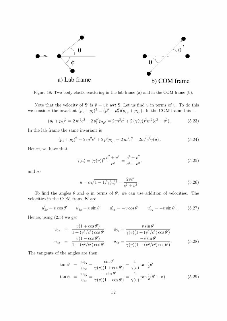
b) COM frame

!

" !

!

’

’

a) Lab frame

Figure 18: Two body elastic scattering in the lab frame (a) and in the COM frame (b).

Note that the velocity of S′ is ~v = vx wrt S. Let us find u in terms of v. To do thiswe consider the invariant (p1 + p2)2 ≡ (pµ1 + pµ2)(p1µ + p2µ). In the COM frame this is

(p1 + p2)2 = 2m2c2 + 2 pµ′

1 p2µ′ = 2m2c2 + 2 (γ(v))2m2(c2 + v2) . (5.23)

In the lab frame the same invariant is

(p1 + p2)2 = 2m2c2 + 2 pµ1p2µ = 2m2c2 + 2m2c2γ(u) . (5.24)

Hence, we have that

γ(u) = (γ(v))2 c2 + v2

c2=c2 + v2

c2 − v2, (5.25)

and so

u = c√

1− 1/γ(u)2 =2vc2

c2 + v2. (5.26)

To find the angles θ and φ in terms of θ′, we can use addition of velocities. Thevelocities in the COM frame S′ are

u′3x = v cos θ′ u′3y = v sin θ′ u′4x = −v cos θ′ u′4y = −v sin θ′ . (5.27)

Hence, using (2.5) we get

u3x =v(1 + cos θ′)

1 + (v2/c2) cos θ′u3y =

v sin θ′

γ(v)(1 + (v2/c2) cos θ′)

u4x =v(1− cos θ′)

1− (v2/c2) cos θ′u4y =

−v sin θ′

γ(v)(1− (v2/c2) cos θ′). (5.28)

The tangents of the angles are then

tan θ =u3y

u3x

=sin θ′

γ(v)(1 + cos θ′)=

1

γ(v)tan 1

2θ′

tanφ =u4y

u4x

=− sin θ′

γ(v)(1− cos θ′)=

1

γ(v)tan 1

2(θ′ + π) . (5.29)

52

5.3 Threshold energies

Suppose that two particles collide, one initially at rest, and a third particle is created.What is the minimum kinetic energy needed? The conservation of momentum equationis

pµ1 + pµ2 = pµ3 + pµ4 + pµ5 . (5.30)

Let us assume that the two incoming particles and the first two outgoing particles havethe same mass m and that the mass of the third outgoing particle is M . The best thingto do is to go into the COM frame. In the COM frame we have that the threshold occurswhen the final particles all have zero spatial momentum. The incoming particles alsohave equal and opposite spatial momentum. Hence, the conservation of energy equationis

mγ(v)c2 +mγ(v)c2 = mc2 +mc2 +Mc2 . (5.31)

Hence, we have

γ(v) = 1 +M

2m(5.32)

The kinetic energy for each incoming particle T is then

T = γ(v)mc2 −mc2 =M

2c2 , (5.33)

in other words the extra energy for each particle is used to create half the rest energy ofthe third particle.

Let us now find how much energy is required in the lab frame. In the lab frame welet the velocity of the first particle be ~u and the second particle is at rest. Hence, wehave that

pµ1 = (mcγ(u),m~uγ(u)) pµ2 = (mc,~0) . (5.34)

We then construct the invariant

p1 · p2 ≡ pµ1p2µ = m2c2γ(u) = m(Tlab +mc2) , (5.35)

where Tlab is the kinetic energy of the first particle in the lab frame. Back in the COMframe, this invariant is

p1 · p2 = m2c2γ(v)2 +m2v2γ(v)2 = 2m2c2γ(v)2 −m2c2 = m2c2

(1 +

2M

m+M2

2m2

)(5.36)

where we used the result in (5.33). Comparing the invariants in the two frames, we find

Tlab = Mc2

(2 +

M

2m

), (5.37)

53

In particular, notice that if M >> m, then

Tlab ≈M2c2

2m, (5.38)

which is much bigger than the rest energy of the third particle. This means that it willtake a tremendous amount of kinetic energy to produce the third particle. The reasonfor the big difference is that in order to conserve the spatial momentum, the new particlewill also have to a lot of kinetic energy, so most of the energy of the incoming particlegoes toward the creation of the third particle’s kinetic energy.

This is why it is much more efficient to build particle colliders where two beams ofparticles smash into each other with equal and opposite momenta, than it is to buildan accelerator where one particle hits another particle at rest. For example, the afore-mentioned LHC collider at CERN is built so that the accelerator is in the COM frameof the two colliding beams of protons. Each beam will eventually have an energy of 7TeV (a TeV is a trillion eV=1000 GeV) so there is 14 TeV of energy available to createparticles. The beam should be powerful enough to create particles with masses perhapsin excess of 1 TeV (The reason why it won’t make a single particle with mass 14 TeVis because the protons themselves are not point particles but are actually a collection ofquarks and gluons). To make a TeV particle when one proton is at rest would requirethat the other proton have a kinetic energy that is in excess of 105 TeV.

5.4 The 4-momentum for photons

Light comes in discrete quanta called photons. Each photon is an individual particle. Itmight seem that constructing a 4-momentum for a photon as we did for other particlesis problematic since photons do not have a rest frame to measure a rest energy in.Nonetheless, previously we saw that the 4-momentum is proportional to the 4-velocity uµ,so we can try the same thing and assume that the photon’s 4-momentum is proportionalto its 4-velocity.

We also saw that the definition for a light ray’s 4-velocity depends on how we pa-rameterize the light’s trajectory. However, one fact is indisputable, namely that the4-velocity is light-like, that is, uµuµ = 0. Therefore, what we will do is let the photon’s4-momentum be pµ with pµpµ = 0. We saw previously for a particle with a rest massm0 that pµpµ = m0c

2. Hence, one can say that a photon has zero rest mass, or that is amassless particle.

Actually quantum mechanics lets us make a more definite statement. The DeBrogliewavelength is given by

λ =h

|~p|, (5.39)

where ~p is the spatial part of the 4-momentum and h is Planck’s constant. A better wayto write this relation is with the wave-vector ~k, in which case we have

~p = ~~k , (5.40)

54

out

!e

!e

!

"

# in

#

Figure 19: A photon with frequency νin scattering off an electron at rest. The outgoing photonhas frequency νout and an angle θ off of the x-axis.

where ~ = h/2π and h = 6.63× 10−34 joule-sec is Planck’s constant. We can now extendthis to the complete 4-vector giving us

pµ = ~ kµ . (5.41)

Recall that we previously found for light waves that kµkµ = 0, so obviously pµ will satisfythe same relation.

In any case, we can express the 4-momentum for a photon as

pµ = (|~p |, ~p) = ~(ω/c,~k) . (5.42)

From this we see that the photon’s energy is ~ω = hν.

5.5 Compton scattering

Suppose we consider a photon with frequency νin scattering off of a charged particle atrest, such as an electron. This is usually an elastic process, although there is a smallbut nonzero probability that more photons will be created, making the process inelastic.In any case, we assume that the process is elastic. Without any loss of generality, weassume that the photon is heading in the x direction and that the photon scatters offwith angle θ in the x− y plane. Momentum conservation then implies that the electronalso scatters off in the x− y plane. The outgoing photon will have frequency νout. Thisprocess is shown in figure 19.

We now show how to find the outgoing frequency in terms of the incoming frequencyand the outgoing angle θ. Conservation of 4-momentum gives us

pµ1 + pµ2 = pµ3 + pµ4 , (5.43)

where pµ1 and pµ3 are the momenta for the photons and pµ2 and pµ4 are the momenta forthe electrons. The first three momenta are

pµ1 =

(hνin

c,hνin

c, 0, 0

)pµ2 = (mec, 0, 0, 0)

pµ3 =

(hνout

c,hνout

ccos θ,

hνout

csin θ, 0

), (5.44)

55

where me is the electron mass. We then bring pµ3 on the other side of the conservationequation and square both side,

(p1 + p2 − p3)2 = (p4)2 , (5.45)

where (p)2 ≡ pµpµ. This then gives

(p1)2 + (p2)2 + (p3)2 + 2p2 · (p1 − p3)− 2p1 · p3 = (p4)2 , (5.46)

where p · q ≡ pµqµ. Using that (p2)2 = (p4)2 and (p1)2 = (p3)2 = 0 we have

2meh(νin − νout) = 2νinνouth

2

c2(1− cos θ) . (5.47)

Dividing both sides of the equation by meνinνouth, multiplying by c and using the trigono-metric identity (1− cos θ) = 2 sin2 1

2θ, we arrive at the expression

c

νout

− c

νin

= 2 sin2 12θ

h

mec(5.48)

This is then rewritten as

λout − λin = 2 sin2 12θ λC ≥ 0 . (5.49)

The quantity λC = h/mec is called the electron’s Compton wavelength. We can also seethat the outgoing photon has a longer wavelength than the incoming photon. It is easyto understand this: the photon has to give up some of its energy to impart kinetic energyto the electron. The longer wavelength has lower energy. One should also observe thatfor scattering in the forward direction where the deflection angle θ is small, the shift inwavelength is also small because of the sin2 1

2θ factor. In fact the shift is largest when

θ = π, which corresponds to a photon being scattered straight back.Plugging in the values for h, c and me, we find

λC =hc

mec2=

(6.6× 10−34 joule-sec)(3× 108 m/sec)

(0.511× 106 eV)(1.6× 10−19 joules/eV)

= 2.4× 10−12 m = .024 A , (5.50)

so we see that the Compton wavelength of an electron is quite a bit shorter than thetypical atomic scale. In fact for ordinary visible light where λ ∼ 5000 A, Comptonscattering will have a miniscule effect on the wavelength. Photons in these wavelengthshave energies on the order of an eV. However, for photons with energies of an MeV theshift in wavelength can be significant. These photons are known as gamma rays and aretypical products in nuclear decays.

5.6 Forces

In this section we generalize the Newtonian force relation in (5.1) to 4-vectors. As wehave done before when we encountered a time derivative of a 3-vector, we replace the

56

3-vector with a 4-vector and the time derivative with a derivative with respect to theproper time τ . Hence, we define the 4-force as

F µ ≡ dpµ

dτ(5.51)

Using time dilation dt = γ(v)dτ , we find that the components of F µ are

F µ =

(γ(v)

dp0

dt, γ(v)

d~p

dt

)= γ(v)

(1

c

dE

dt, ~f

). (5.52)

Hence, the first component is related to the rate of change of the energy, while the spatialparts is the usual force ~f multiplied by a γ factor.

Now notice further that

F µ =d

dτ(m0u

µ) = m0aµ + uµ

dm0

dτ. (5.53)

If we now take the scalar product of F µ with uµ we get

u · F = uµFµ = m0u · a+ u · u dm0

dτ= 0 +

d(m0c2)

dτ. (5.54)

If we now take the scalar product using the explicit components in (4.15) and (5.52), weget

u · F = γ(v)2

(dE

dt− ~v · ~f

). (5.55)

Thus, comparing eqs. (5.54) and (5.55) we derive the relation

dE

dt= ~v · ~f +

1

γ(v)

d(m0c2)

dt. (5.56)

In other words, the rate of change of the energy is given by the usual ~v · ~f term we havein Newtonian mechanics, plus a term corresponding to the rate of change of the restenergy of the body.

A pure force is one that does not change the rest energy. We can see from (5.54) thata pure force has u · F = 0. A heatlike force is one which does not change the particle’svelocity. In the case of the pure force, dE

dtcan be expressed as

dE

dt=d~x

dt· ~f =

d

dt(~x · ~f) =

dW

dt, (5.57)

where W is the work done on the system and we have used that ~f has no explicit tdependence.

In Newtonian mechanics, a conservative force (that is, one with no frictional forces)can be written as the derivative of a potential Φ as follows:

~f = −~∇Φ . (5.58)

57

Let us now show that there is no equivalent for a pure 4-force, in other words, it is notpossible to write Fµ = ∂µΦ if the force is nonzero. To show this, assume that Fµ doestake this form. Then we have

0 = uµFµ = uµ∂uΦ =dxµ

dτ

∂Φ

∂xµ=dΦ

dτ. (5.59)

This only has a solution if Φ is a constant, and so the only solution has Fµ = 0.Newtonian mechanics is of course not complete without Newton’s second law,

~f = m~a . (5.60)

Hence the acceleration is always parallel to the force. The same thing does not hold truefor the 4-force and 4-acceleration. Let us again assume that we have a pure force. Using(5.1) we have

d

dt(m0γ~v) = m0γ ~a+ ~v

d

dt(m0γ) = m0γ ~a+

~v

c2

dE

dt. (5.61)

For a pure force we also have

dE

dt= ~v · ~f , (5.62)

so combining this with the previous equation we get

~f = m0γ ~a+~v

c2(~v · ~f) . (5.63)

Consequently, ~f is parallel to ~a only if, either ~f is parallel to ~v, or ~v · ~f = 0. Let us write~f as

~f = ~f|| + ~f⊥ , (5.64)

where ~f|| is the part of ~f that is parallel to ~v and ~f⊥ is the part that is perpendicular to~v. For the parallel part we have

~f|| = ~f|| = m0γ ~a|| +v2

c2~f|| , (5.65)

where ~a|| is the component of ~a that is parallel to ~v. From (5.65) it follows that

~f|| =m0γ

1− v2/c2~a|| = m0γ

3~a|| . (5.66)

For the perpendicular part, we clearly have

~f⊥ = m0γ ~a⊥ (5.67)

Since the proportionality constant is different between the parallel and perpendicularparts of ~f and ~v, ~f and ~a are in general not parallel to each other. Of course in thenonrelativistic limit v2/c2 << 1, then γ ≈ 1 and the proportionality factors become the

same, in which case ~f and ~a are parallel.

58

6 Electromagnetism (Introduction)

After making a few minimal assumptions and invoking Occam’s razor we can derive thelaws of electrodynamics, and in particular Maxwell’s equations, more or less from firstprinciples. We will start by trying to find a force law for charged particles. We makethree assumptions:

1. The electromagnetic force ~f is covariant. In other words it is part of a 4-force F µ

where F µ = γ (dE/cdt, ~f).

2. The force is proportional to the particle’s charge q.

3. The electrodynamic force should not change the rest energy of the particles, afterall,an electron in an electromagnetic field stays an electron with the same rest energy.Thus, the force is a pure force and so uµFµ = 0.

The first thing we observe is that the force must be velocity dependent, otherwise wecould choose an arbitrary timelike uµ such that uµFµ 6= 0. We now make one furtherassumption: we want the velocity dependence to be as simple as possible (this is theOccam’s razor part), so we choose it to be linear in uµ. Hence, a covariant 4-forcesatisfying all of these properties can be written as

Fµ =q

cEµν u

ν (6.1)

where the c is put in for later convenience and Eµν has no q dependence. Eµν has to havetwo lower indices in order to map the contravariant vector uµ to the covariant vector Fµ.The pure force condition gives

Eµν uµ uν = 0 (6.2)

for all uµ. But this is only possible if Eµν is antisymmetric. It is straightforward to showthat an antisymmetric tensor does give zero:

Eµν uµ uν = −Eνµ uµ uν = −Eνµ uν uµ = −Eµν uµ uν , (6.3)

where in the last step we simply relabeled the dummy indices. Hence, Eµν uµ uν is equal

to minus itself, which is possible only if it is zero. We have previously seen at the end ofsection 3 that an antisymmetric tensor is antisymmetric in all frames, so (6.1) is indeeda covariant equation. We will call Eµν the electromagnetic field7.

6.1 The field equations

We next assume that the fields couple to currents. The electric current is written as ~jand is equal to the charge flow per unit time and unit area along the direction of its flow.

7Most textbooks use the symbol Fµν for the field, but we are following Rindler’s notation. Besides,Fµ is reserved for the force, so to minimize confusion we will stick to Eµν .

59

!

!

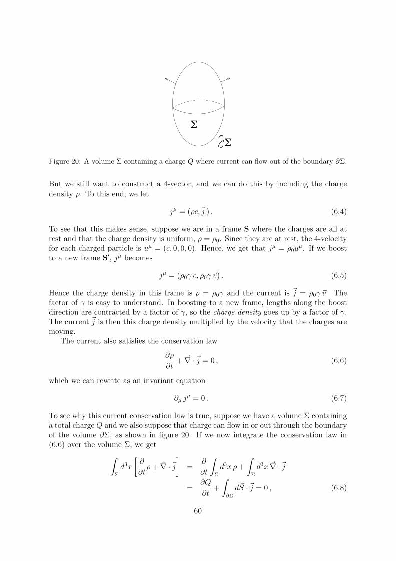
Figure 20: A volume Σ containing a charge Q where current can flow out of the boundary ∂Σ.

But we still want to construct a 4-vector, and we can do this by including the chargedensity ρ. To this end, we let

jµ = (ρc,~j ) . (6.4)

To see that this makes sense, suppose we are in a frame S where the charges are all atrest and that the charge density is uniform, ρ = ρ0. Since they are at rest, the 4-velocityfor each charged particle is uµ = (c, 0, 0, 0). Hence, we get that jµ = ρ0u

µ. If we boostto a new frame S′, jµ becomes

jµ = (ρ0γ c, ρ0γ ~v) . (6.5)

Hence the charge density in this frame is ρ = ρ0γ and the current is ~j = ρ0γ ~v. Thefactor of γ is easy to understand. In boosting to a new frame, lengths along the boostdirection are contracted by a factor of γ, so the charge density goes up by a factor of γ.The current ~j is then this charge density multiplied by the velocity that the charges aremoving.

The current also satisfies the conservation law

∂ρ

∂t+ ~∇ ·~j = 0 , (6.6)

which we can rewrite as an invariant equation

∂µ jµ = 0 . (6.7)

To see why this current conservation law is true, suppose we have a volume Σ containinga total charge Q and we also suppose that charge can flow in or out through the boundaryof the volume ∂Σ, as shown in figure 20. If we now integrate the conservation law in(6.6) over the volume Σ, we get∫

Σ

d3x

[∂

∂tρ+ ~∇ ·~j

]=

∂

∂t

∫Σ

d3x ρ+

∫Σ

d3x ~∇ ·~j

=∂Q

∂t+

∫∂Σ

d~S ·~j = 0 , (6.8)

60

where we have used Gauss’ law to relate the volume integral of a divergence to a surfaceintegral. The meaning of this equation is that the rate of change of the charge Q insideΣ is minus the rate that the charge is flowing out. If no charge is created or destroyed,then this will be true. So current conservation is basically a statement that the totalcharge is conserved.

We now look for a field equation that satisfies current conservation. The simplestsuch equation one can write down is

∂µEµν = κ jν , (6.9)

where κ is a constant to be determined later8. To see that this is consistent with currentconservation, let us take a ∂ν derivative on both sides of (6.9). This gives

∂µ∂ν Eµν = κ ∂νj

ν . (6.10)

The right hand side of (6.10) is zero. Using the commutativity of the derivatives (theirorder does not matter) and the antisymmetry of Eµν , the left hand side of (6.10) satisfies

∂µ∂ν Eµν = ∂ν∂µE

µν = −∂ν∂µEνµ = −∂µ∂ν Eµν , (6.11)

where the last step is just a relabeling of the dummy indices. Just like in (6.3), we get anexpression that is minus itself, and so it is zero. Hence, (6.9) is consistent with currentconservation.

6.2 Maxwell’s equations: part 1

The field equation (6.9) is actually four equations since there is one free index in theequation. We now show that this is equivalent to half of Maxwell’s equations.

We first note that because of its antisymmetry, the field Eµν has six independentcomponents. Let’s count them: If we set µ = ν then Eµν = −Eµν and thus we have tochoose µ 6= ν in order to get a nonzero component. In this case we still have Eµν = −Eνµ,so we can choose µ < ν to list all the components, since the µ > ν case is related tothe µ < ν case by the antisymmetry relation. Hence there are 3+2+1=6 six differentchoices.

We define the components as follows: Three of the components are

E0i = ei , i = 1, 2, 3 . (6.12)

The other three are

Eij = −c εijk bk , (6.13)

where εijk is completely antisymmetric under the exchange of any two indices and hasε123 = 1. The repeated k index is assumed to be summed over, even though I have shown

8Notice that the field has raised indices in (6.9), which one gets by using two η tensors: Eµν =ηµληνρEλρ

61

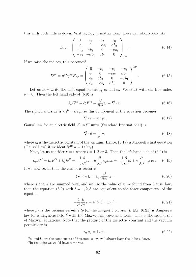
this with both indices down. Writing Eµν in matrix form, these definitions look like

Eµν =

0 e1 e2 e3

−e1 0 −c b3 c b2

−e2 c b3 0 −c b1

−e3 −c b2 c b1 0

µν

. (6.14)

If we raise the indices, this becomes9

Eµν = ηµληνσEλσ =

0 −e1 −e2 −e3

e1 0 −c b3 c b2

e2 c b3 0 −c b1

e3 −c b2 c b1 0

µν

. (6.15)

Let us now write the field equations using ei and bi. We start with the free indexν = 0. Then the left hand side of (6.9) is

∂µEµ0 = ∂iE

i0 =∂

∂xiei = ~∇ · ~e . (6.16)

The right hand side is κ j0 = κ c ρ, so this component of the equation becomes

~∇ · ~e = κ c ρ . (6.17)

Gauss’ law for an electric field, ~e, in SI units (Standard International) is

~∇ · ~e =1

ε0ρ , (6.18)

where ε0 is the dielectric constant of the vacuum. Hence, (6.17) is Maxwell’s first equation(Gauss’ Law) if we identify10 κ = 1/(cε0).

Next, let us consider ν = i where i = 1, 2 or 3. Then the left hand side of (6.9) is

∂µEµi = ∂0E

0i + ∂jEji = −1

c

∂

∂tei − c

∂

∂xjεjik bk = −1

c

∂

∂tei + c

∂

∂xjεijk bk . (6.19)

If we now recall that the curl of a vector is

(~∇×~b )i = εijk∂

∂xjbk , (6.20)

where j and k are summed over, and we use the value of κ we found from Gauss’ law,then the equation (6.9) with i = 1, 2, 3 are equivalent to the three components of theequation

− 1

c2

∂

∂t~e+ ~∇×~b = µ0

~j , (6.21)

where µ0 is the vacuum permitivity (or the magnetic constant). Eq. (6.21) is Ampere’s

law for a magnetic field ~b with the Maxwell improvement term. This is the second setof Maxwell equations. Note that the product of the dielectric constant and the vacuumpermitivity is

ε0 µ0 = 1/c2 . (6.22)

9ei and bi are the components of 3-vectors, so we will always leave the indices down.10In cgs units we would have κ = 4π/c.

62

6.3 The field potential, gauge invariance and the Bianchi iden-tity

To help find the rest of Maxwell’s equations, we introduce a new field, the gauge potentialAµ. The field Eµν can be expressed in terms of Aµ as

Eµν = ∂µAν − ∂νAµ . (6.23)

Notice that this expression is manifestly antisymmetric under the exchange of µ and ν.Plugging this expression into the field equations we find the new equation

�Aν − ∂ν∂ · A =1

cε0jν , (6.24)

where � = ∂µ∂µ and ∂ · A = ∂µAµ.

While we have introduced the gauge potential Aµ, the physical fields are still the

electric and magnetic fields, ~e and ~b. In fact, if we make the transformation Aµ →Aµ + ∂µΦ, where Φ is an arbitrary scalar field, then

Eµν → ∂µAν − ∂νAµ + ∂µ∂νΦ− ∂ν∂µΦ = Eµν . (6.25)

The field Eµν , and hence ~e and ~b, are invariant under this transformation. Such atransformation is called a gauge transformation. Unlike, say, a Lorentz transformation,under a gauge transformation, all physical quantities are unchanged. Therefore, we canmake a gauge transformation to simplify equations without affecting the physics. Forexample, we can choose a Φ, such that after the transformation the gauge potentialsatisfies the equation ∂ ·A = 0. Such a condition is called a gauge choice. This particulargauge choice is called the Lorenz gauge 11.

Assuming (6.23), we have the following relation:

∂λEµν + ∂ν Eλµ + ∂µEνλ = 0 . (6.26)

To see this explicity, we substitute in the gauge potential into the left hand side of (6.26),after which we find

∂λ(∂µAν − ∂νAµ) + ∂ν(∂λAµ − ∂µAλ) + ∂µ(∂νAλ − ∂λAν)= ∂λ∂µAν − ∂µ∂λAν + ∂ν∂λAµ − ∂λ∂νAµ + ∂µ∂νAλ − ∂ν∂µAλ = 0 . (6.27)

The equation in (6.26) is called the Bianchi identity. Actually, this is four equations,since if any of the three free indices are the same then the equation is manifestly zerostrictly from the antisymmetry of Eµν . Hence, we only have new relations if all threeindices are different and there are four ways to choose three distinct indices from fourpossible values.

11Notice that Lorenz is different than Lorentz. Hendrik Lorentz (as in Lorentz transformation) wasa Dutch phyiscist, while Ludvig Lorenz was Danish. Nevertheless, a common mistake, even in manyfamous textbooks, is to call this the Lorentz gauge.

63

6.4 Maxwell’s equations: part 2

We now show that the Bianchi identity gives the rest of Maxwell’s equations. Let usstart by choosing λ, µ, ν =1,2,3 respectively in (6.26). Hence this gives

∂1E23 + ∂2E31 + ∂3E12 = −c(

∂

∂x1b1 +

∂

∂x2b2 +

∂

∂x3b3

)= 0 . (6.28)

This then gives the Maxwell equation

~∇ ·~b = 0 , (6.29)

which means that there are no magnetic monopole charges in nature.Now choose λ, µ, ν =0,1,2 respectively in (6.26). This results in

∂0E12 + ∂2E01 + ∂1E20 =1

c

∂

∂t(−c b3) +

∂

∂x2e1 −

∂

∂x1e2 = −

(∂

∂t~b+ ~∇× ~e

)3

= 0 .(6.30)

This, along with similar equations for λ, µ, ν =0,2,3 and λ, µ, ν =0,3,1 result in Faraday’slaw for the electric field resulting from a time dependent magnetic field,

∂

∂t~b+ ~∇× ~e = 0 . (6.31)

These are the last three Maxwell equations.

6.5 The electromagnetic wave

With the Lorenz gauge, the field equations in (6.24) simplify to

�Aν =1

c ε0jν . (6.32)

In a vacuum there are no charges or currents, thus jµ = 0. In this case, this equationbecomes a simple wave equation

�Aν =1

c2

∂2

∂t2Aν − ~∇ · ~∇Aν = 0 . (6.33)

Each component of Aν is a solution to the same equation. One particular solution tothis equation is

Aν(t, ~x) = Aν(~k) eiω(k)t−i~k·~x

= Aν(~k) eikµxµ

, (6.34)

where ω(~k) = c|~k| and in the second line we used that kµ = (ω/c,−~k ). Hence, this is

a wave traveling at the speed of light. In fact, it is a light wave! The choice of ~k givesthe wavelength and direction for the wave, while Aν(~k) is the amplitude. Since the wave

64

equation is linear, a general solution is a sum over all possible values of the wave-vector~k. Since ~k can be anything, the sum is actually an integral and has the form

Aν(t, ~x) =

∫d3~k

(2π)3Aν(~k) eikµx

µ

, (6.35)

where the factor of 1/(2π)3 is a standard normalization factor when integrating overwave vectors.

It might seem that there are four independent waves for a given ~k since there are fourchoices for ν. But the Lorenz gauge leads to the condition

∂νAν(~k)eikµx

µ

= 0 = ikνAν(~k)eikµx

µ

⇒ kνAν(~k) = k · A(~k) = 0 . (6.36)

A general solution to this is

Aν(~k) = Φ(~k)kν + Aν⊥(~k) , (6.37)

where Φ(~k) is arbitrary, A0⊥(~k) = 0 and ~k · ~A⊥(~k) = 0. (Note that Aµ⊥ = (A0

⊥,~A⊥).) The

first term on the right hand side is a pure gauge term – it makes no contribution to ~eand ~b. This is easy to check:

∂µkνΦ(~k)eikλxλ − ∂νkµΦ(~k)eikλx

λ

= i(kµkν − kνkµ)Φ(~k)eikλxλ

= 0 . (6.38)

Hence, the only physical components are the two independent components in ~A⊥(~k) that

are orthogonal to ~k. The direction of ~A⊥(~k) is called the polarization of the light wave.

Let us now find the ~e and ~b fields in terms of ~A⊥(~k). If we let

~e (t, ~x) =

∫d3~k

(2π)3~e (~k) eikµx

µ

,

~b (t, ~x) =

∫d3~k

(2π)3~b (~k) eikµx

µ

, (6.39)

then equation (6.23) and the identifications in (6.14) leads to the relations

~e (~k) = −i ωc~A⊥(~k)

~b (~k) = − ic~k × ~A⊥(~k) =

1

ω~k × ~e (~k) . (6.40)

Thus, both ~e and ~b are perpendicular to the direction of the wave and they are perpen-dicular to each other as well.

6.6 Lorentz transformations of ~e and ~b

The fields ~e and ~b are part of an antisymmetric(

02

)tensor, and so their transformation

properties are different than if they were each part of a covariant vector. In particular,the tensor in frame S′ is

Eµ′ν′ = Λµµ′Λ

νν′Eµν . (6.41)

65

If the Lorentz transformation is the boost in the x-direction as given in (3.10), then thevarious components of the fields are as follows:

e′1 = E0′1′ = Λµ0′Λ

ν1′Eµν = Λ0

0′Λ1

1′E01 + Λ10′Λ

01′E10 = γ2e1 +

(vcγ)2

(−e1) = e1

e′2 = E0′2′ = Λµ0′Λ

ν2′Eµν = Λ0

0′Λ2

2′E02 + Λ10′Λ

22′E12 = γe2 +

v

cγ(−cb3) = γ(e2 − vb3)

e′3 = E0′3′ = Λµ0′Λ

ν3′Eµν = Λ0

0′Λ3

3′E03 + Λ10′Λ

33′E13 = γe3 +

v

cγ(+cb2) = γ(e3 + vb2)

b′1 = −1

cE2′3′ = −1

cΛµ

2′Λν

3′Eµν = −1

cΛ2

2′Λ3

3′E23 = b1

b′2 = −1

cE3′1′ = −1

cΛµ

3′Λν

1′Eµν = −1

cΛ3

3′Λ1

1′E31 −1

cΛ3

3′Λ0

1′E30 = γ(b2 +v

c2e3)

b′3 = −1

cE1′2′ = −1

cΛµ

1′Λν

2′Eµν = −1

cΛ1

1′Λ2

2′E12 −1

cΛ0

1′Λ2

2′E02 = γ(b3 −v

c2e2) .

(6.42)

Notice that the components along the boost direction, e1 and b1 are unchanged underthe boost, while those that are transverse end up mixing the ~e and ~b fields together.

6.7 Invariants

Let us now look for scalar invariants of the electromagnetic fields. Since Eµν has twoindices, one invariant we can write down is Eµνη

µν . However, since Eµν is antisymmetricand ηµν is symmetric, the invariant is zero. This is still an invariant, it just happens tobe a trivial one.

Next, we consider a product of Eµν fields. In this case we can construct the invariant

EµνEµν = EµνEλρη

µληνρ

= 23∑i=1

(E0i)2η00ηii + 2

3∑1≤i<j

(Eij)2ηiiηjj = −2

3∑i=1

(E0i)2 + 2

3∑1≤i<j

(Eij)2

= −2 (~e · ~e− c2~b ·~b ) , (6.43)

where we have used the symmetry that EµνEµν = EνµEνµ and we have only includedthose terms in the sum that are nonzero. From this invariant we can infer a few usefulfacts. For example, if in one frame we have ~e 6= 0 and ~b = 0, then in no frame is theelectric field zero. To see this, we note that ~e · ~e − c2~b ·~b > 0 in this frame. But sincethis is an invariant, it is true in all frames. Hence |~e | > c |~b| in all frames. Hence |~e | > 0

in all frames. We can also say a similar thing if ~e · ~e− c2~b ·~b < 0 or ~e · ~e− c2~b ·~b = 0.There is another invariant that is quadratic in Eµν . But to build this, we need to

introduce another tensor, called the ε-tensor (“epsilon tensor”), εµνλσ. This tensor isdefined to be completely antisymmetric

εµνλσ = −ενµλσ = −ελνµσ = −εσνλµ (6.44)

and is normalized to

ε0123 = 1 . (6.45)

66

Since it is antisymmetric, all indices have to be different for εµνλσ to be nonzero. Let usnow show that εµνλσ is a

(04

)tensor. Consider the determinant of any Lorentz transfor-

mation matrix Λµµ′ . The determinant is always 1 and a little thought reveals that

det Λ = 1 = Λµ0′Λ

ν1′Λ

λ2′Λ

σ3′ εµνλσ . (6.46)

One can also check that the interchange of any two primed indices changes the sign ofthe expression on the right hand side. Hence, we have that

Λµµ′Λ

νν′Λ

λλ′Λ

σσ′ εµνλσ = εµ′ν′λ′σ′ , (6.47)

and so εµνλσ indeed transforms as a tensor.With the ε-tensor we can then construct the invariant

EµνEλσεµνλσ = 8(E01E23 + E02E31 + E03E12) = 8c(e1b1 + e2b2 + e3b3)

= 8 c~e ·~b , (6.48)

where we used the antisymmetry of the tensors involved. Hence, ~e · ~b is a Lorentzinvariant. Therefore if ~e ·~b = 0 in one frame, it is zero in all frames.

6.8 The Lorentz force

Let us return to the force equation in (6.1). If we substitute for Eµν the components in(6.14), then for the ith spatial component of Fµ we have

Fi = −γfi =q

cEiλu

λ =q

c(Ei0u

0 +3∑j=1

Eijuj) =

q

cγ (−cei − c

3∑j,k=1

εijkvjbk)

= −q γ (ei + (~v ×~b )i) . (6.49)

Hence, we arrive at the Lorentz force equation

~f = q (~e+ ~v ×~b ) . (6.50)

Let’s use the Lorentz force equation to compute how strong the magnetic fields willbe at the LHC when the proton energies are 7 TeV. The protons are traveling in a circle,so while |~p| is not changing in time, the direction of ~p is. In particular, we have that∣∣∣∣d~pdt

∣∣∣∣ =|~v |R|~p | , (6.51)

where R is the radius of the ring. As we have seen, the protons are moving very close tothe speed of light, so we can replace |~v | with c, and then write∣∣∣∣d~pdt

∣∣∣∣ ≈ m0c2γ

R=

7 TeV

27/(2π) km=

7× 1.6× 10−7 joules

4.29× 103 m= 2.6× 10−10 joules/m . (6.52)

67

The charge of the proton in SI units is q = +1.6×10−19 coulombs. Hence the magnitudeof the ~b field is

|~b | ≈ 1

qc

∣∣∣∣d~pdt∣∣∣∣ =

1

(1.6× 10−19 coulombs)(3× 108 m/s)2.6× 10−10 joules/m = 5.4 tesla ,

(6.53)

which is 50,000 times stronger than the earth’s magnetic field. Actually, this field is theaverage field needed around the ring. In reality, the LHC has 1232 magnets of length14.3 m each. You can quickly check that the total length of the magnets is 17.6 km,covering about 65 % of the ring. Therefore, the field inside each magnet should be

(5.4 tesla) × (27 km/17.6 km) = 8.3 tesla . (6.54)

For the time component of Fµ we have

F0 =γ

c

dE

dt=q

cE0λu

λ =q

c

3∑j=1

E0juj) =

qγ

c~e · ~v . (6.55)

Hence,

dE

dt= q ~e · ~v . (6.56)

Notice that the magnetic field does not change the energy. Since the electromagneticforce is a pure force, the change in energy is a change in kinetic energy only. In fact, wecould have derived this from (5.57), where

dE

dt= ~v · ~f = q ~v · (~e+ ~v ×~b ) = q ~v · ~e , (6.57)

since ~v is perpendicular to ~v × ~w, where ~w is any vector.

68

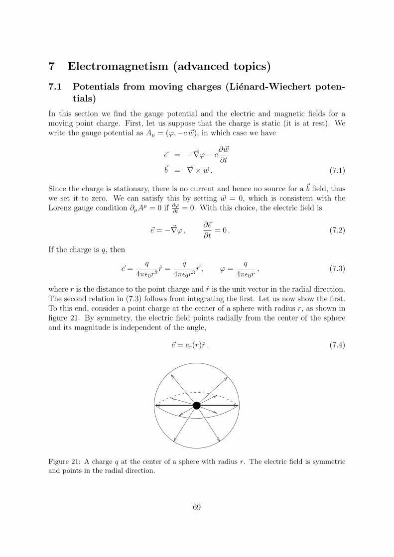
7 Electromagnetism (advanced topics)

7.1 Potentials from moving charges (Lienard-Wiechert poten-tials)

In this section we find the gauge potential and the electric and magnetic fields for amoving point charge. First, let us suppose that the charge is static (it is at rest). Wewrite the gauge potential as Aµ = (ϕ,−c ~w), in which case we have

~e = −~∇ϕ− c∂ ~w∂t

~b = ~∇× ~w . (7.1)

Since the charge is stationary, there is no current and hence no source for a ~b field, thuswe set it to zero. We can satisfy this by setting ~w = 0, which is consistent with theLorenz gauge condition ∂µA

µ = 0 if ∂ϕ∂t

= 0. With this choice, the electric field is

~e = −~∇ϕ , ∂~e

∂t= 0 . (7.2)

If the charge is q, then

~e =q

4πε0r2r =

q

4πε0r3~r , ϕ =

q

4πε0r, (7.3)

where r is the distance to the point charge and r is the unit vector in the radial direction.The second relation in (7.3) follows from integrating the first. Let us now show the first.To this end, consider a point charge at the center of a sphere with radius r, as shown infigure 21. By symmetry, the electric field points radially from the center of the sphereand its magnitude is independent of the angle,

~e = er(r)r . (7.4)

Figure 21: A charge q at the center of a sphere with radius r. The electric field is symmetricand points in the radial direction.

69

Q

0

x1

!

xµ

P

x

Figure 22: The world-line for a moving charge q. Given the coordinate xµ at space-time pointQ, τ is chosen so that yµ(τ) is the coordinate at P.

Integrating Gauss’ law in eq. (6.18) over the volume of the sphere, gives∫V

d3x ~∇ · ~e =

∫V

d3xρ

ε0

Gauss′Law(of calculus)

⇒∫∂V

d~S · ~e =q

ε0

4πr2er =q

ε0, (7.5)

where we used that the surface area of the sphere is 4πr2. The first equation in (7.3)then follows.

Now assume that the charge is moving, and that its position as a function of itsproper time is yµ(τ). From this, we want to find the fields at the space-time position Qwith coordinate xµ. Let us define ∆xµ = xµ − yµ(τ), where τ is chosen such that ∆xµ

is light-like, that is, ∆xµ∆xµ = 0. This is shown in the space-time diagram in figure22. In the figure, the event Q is on a light-like trajectory originating out of the event P.Hence τ in ∆xµ is chosen so that yµ(τ) is at P. Since P is in the past of Q, P is calledthe retarded event.

Let us now look for a gauge potential Aµ which is consistent with (7.3) when theparticle is at rest. To this end we let

∆xµ = (ct, ~r ) , (7.6)

where ct = r so that ∆xµ is light-like. We also define D = ∆xµuµ, where uµ is the

4-velocity of the charged particle at the retarded event P. We then let

Aµ =q uµ

4πε0D, (7.7)

70

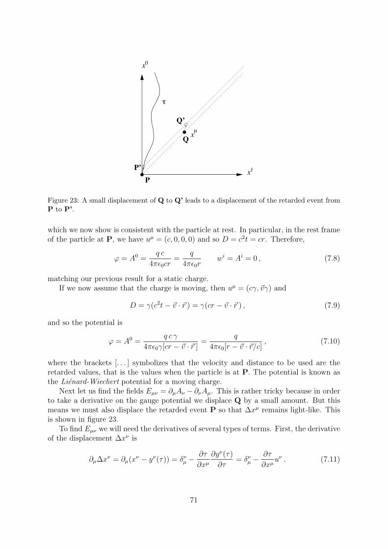
P’

0

x1

!

xµ

P

Q

Q’

x

Figure 23: A small displacement of Q to Q’ leads to a displacement of the retarded event fromP to P’.

which we now show is consistent with the particle at rest. In particular, in the rest frameof the particle at P, we have uµ = (c, 0, 0, 0) and so D = c2t = cr. Therefore,

ϕ = A0 =q c

4πε0cr=

q

4πε0rwi = Ai = 0 , (7.8)

matching our previous result for a static charge.If we now assume that the charge is moving, then uµ = (cγ,~vγ) and

D = γ(c2t− ~v · ~r ) = γ(cr − ~v · ~r ) , (7.9)

and so the potential is

ϕ = A0 =q c γ

4πε0γ[cr − ~v · ~r ]=

q

4πε0[r − ~v · ~r/c], (7.10)

where the brackets [. . . ] symbolizes that the velocity and distance to be used are theretarded values, that is the values when the particle is at P. The potential is known asthe Lienard-Wiechert potential for a moving charge.

Next let us find the fields Eµν = ∂µAν − ∂νAµ. This is rather tricky because in orderto take a derivative on the gauge potential we displace Q by a small amount. But thismeans we must also displace the retarded event P so that ∆xµ remains light-like. Thisis shown in figure 23.

To find Eµν we will need the derivatives of several types of terms. First, the derivativeof the displacement ∆xν is

∂µ∆xν = ∂µ(xν − yν(τ)) = δνµ −∂τ

∂xµ∂yν(τ)

∂τ= δνµ −

∂τ

∂xµuν . (7.11)

71

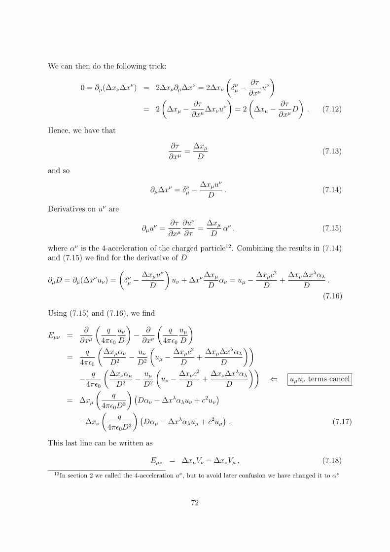
We can then do the following trick:

0 = ∂µ(∆xν∆xν) = 2∆xν∂µ∆xν = 2∆xν

(δνµ −

∂τ

∂xµuν)

= 2

(∆xµ −

∂τ

∂xµ∆xνu

ν

)= 2

(∆xµ −

∂τ

∂xµD

). (7.12)

Hence, we have that

∂τ

∂xµ=

∆xµD

(7.13)

and so

∂µ∆xν = δνµ −∆xµu

ν

D. (7.14)

Derivatives on uν are

∂µuν =

∂τ

∂xµ∂uν

∂τ=

∆xµD

αν , (7.15)

where αν is the 4-acceleration of the charged particle12. Combining the results in (7.14)and (7.15) we find for the derivative of D

∂µD = ∂µ(∆xνuν) =

(δνµ −

∆xµuν

D

)uν + ∆xν

∆xµD

αν = uµ −∆xµc

2

D+

∆xµ∆xλαλD

.

(7.16)

Using (7.15) and (7.16), we find

Eµν =∂

∂xµ

(q

4πε0

uνD

)− ∂

∂xν

(q

4πε0

uµD

)=

q

4πε0

(∆xµανD2

− uνD2

(uµ −

∆xµc2

D+

∆xµ∆xλαλD

))− q

4πε0

(∆xναµD2

− uµD2

(uν −

∆xνc2

D+

∆xν∆xλαλ

D

))⇐ uµuν terms cancel

= ∆xµ

(q

4πε0D3

)(Dαν −∆xλαλuν + c2uν

)−∆xν

(q

4πε0D3

)(Dαµ −∆xλαλuµ + c2uµ

). (7.17)

This last line can be written as

Eµν = ∆xµVν −∆xνVµ , (7.18)

12In section 2 we called the 4-acceleration aν , but to avoid later confusion we have changed it to αν

72

where

Vν =q

4πε0D3

(Dαν −∆xλαλuν + c2uν

). (7.19)

We now want to express the fields in terms of the 3-velocity and 3-acceleration. Recallthat uν = (γc, γ~v ) and

αν =duν

dτ= γ

duν

dτ= γ

(d

dt(γc),

d

dt(γ~v )

)= uµ

dγ

dt+ γ2(0,~a) , (7.20)

where ~a = ddt~v. Notice that Duν − ∆xλuλuν = 0, thus the first term in (7.20) will not

contribute to Vν . Hence, from now on we drop it and simply set αν = γ2(0,−~a ) (theminus sign appears because we lowered the index.) Thus, using (7.6) we have that

∆xλαλ = −γ2~a · ~r . (7.21)

Using this along with the expression for D in (7.9) and the components of uν and αν wefind

V0 =q

4πε0

[γ3c~a · ~r + γc3

γ3c3(r − ~v · ~r/c)3

]=

q

4πε0c2

[~a · ~r + γ−2c2

(r − ~v · ~r/c)3

]~V =

q

4πε0

[−γ3c(r − ~v · ~r/c)~a− γ3(~a · ~r )~v − γc2~v

γ3c3(r − ~v · ~r/c)3

]= − q

4πε0c2

[(r − ~v · ~r/c)~a+ (~a · ~r )~v/c+ γ−2c~v

(r − ~v · ~r/c)3

], (7.22)

where the components of Vµ are Vµ = (V0, ~V ). The square brackets still mean that theretarded values are being used. The components of the electric field are

ei = E0i = ∆x0Vi −∆xiV0 = rVi + riV0 , (7.23)

hence the electric field is

~e = r~V + V0~r

=q

4πε0c2

[(~a · ~r )(~r − r~v/c)− r(r − ~v · ~r/c)~a

(r − ~v · ~r/c)3

]+

q

4πε0

[(~r − r~v/c)

γ2(r − ~v · ~r/c)3

](7.24)

= ~erad + ~enr

We have broken up the ~e field into two pieces, ~erad and ~enr, where the subscripts standfor radiative and nonradiative respectively. The first term, ~erad falls off as 1/r while thesecond term, ~enr falls off as 1/r2. Notice as well that ~erad is linear in ~a while ~enr has no~a dependence.

The components of the ~b field are

bi = − 1

2cεijkEjk = − 1

2cεijk(∆xjVk −∆xkVj) =

1

cεijkrjVk , (7.25)

73

where the repeated j and k indices are summed over. Thus we have that ~b is

~b =1

c~r × ~V . (7.26)

If we now compare to ~e in the first line of (7.24) and use that ~r × ~r = 0, we find that

~b =1

rc(~r × ~e ) . (7.27)

Because of its form in (7.27), ~b satisfies ~r·~b = 0 (for any vectors ~A and ~B, ~A·( ~A× ~B) = 0).

It is also clear that ~b · ~e = 0. In general ~r · ~e 6= 0, however it is straightforward to checkthat ~r · ~erad = 0.

7.2 Example 1: The uniformly moving point charge

We now apply our results derived in the last section. Our first example is a point chargeq moving with constant velocity ~v = vx along the x axis. Let us further suppose thatthere is an observer measuring the field from the point charge on the y axis. We let ∆xν

be the simultaneous displacement (in the observer’s frame) between the observer and thecharge. Hence we can write

∆xν = (0, ~r0) = (0, r0 cos θ, r0 sin θ, 0) , (7.28)

and so r0 is the simultaneous distance between the observer and the charge. Note that∆xν is not the displacement between the observer and the retarded event ∆xν that wasdiscussed at length in the previous section. This displacement is

∆xν = (r, ~r ) = (r, r cosφ, r sinφ, 0) . (7.29)

Figure 24 shows these different distances and angles between the charge and the observer.In the figure the observer is making the measurement at space-time point Q, P is theretarded event for the point charge and R is the simultaneous event. The displacement~d shows the movement of the charge between the time of the retarded event and the timeof event Q. This elapsed time is ∆t = r/c and so ~d = ~v∆t = r~v/c. From the figure we

can see that ~r0 = ~r − ~d = ~r − r~v/c.Since the charge has no acceleration, the electric field is

~e = ~enr =q

4πε0

[(~r − r~v/c)

γ2(r − ~v · ~r/c)3

]=

q

4πε0γ2

(~r − r~v/c)(~r · (~r − r~v/c)/r)3

=q

4πε0γ2

~r0

(~r · ~r0)3/r3. (7.30)

Interestingly, the electric field points along ~r0, that is between the simultaneous positionof the charge and the observer, as opposed to the retarded position.

74

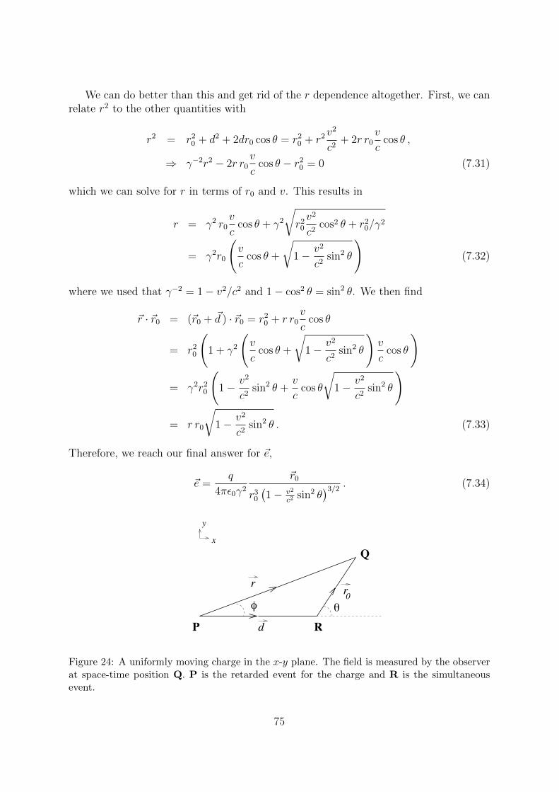
We can do better than this and get rid of the r dependence altogether. First, we canrelate r2 to the other quantities with

r2 = r20 + d2 + 2dr0 cos θ = r2

0 + r2v2

c2+ 2r r0

v

ccos θ ,

⇒ γ−2r2 − 2r r0v

ccos θ − r2

0 = 0 (7.31)

which we can solve for r in terms of r0 and v. This results in

r = γ2 r0v

ccos θ + γ2

√r2

0

v2

c2cos2 θ + r2

0/γ2

= γ2r0

(v

ccos θ +

√1− v2

c2sin2 θ

)(7.32)

where we used that γ−2 = 1− v2/c2 and 1− cos2 θ = sin2 θ. We then find

~r · ~r0 = (~r0 + ~d ) · ~r0 = r20 + r r0

v

ccos θ

= r20

(1 + γ2

(v

ccos θ +

√1− v2

c2sin2 θ

)v

ccos θ

)

= γ2r20

(1− v2

c2sin2 θ +

v

ccos θ

√1− v2

c2sin2 θ

)

= r r0

√1− v2

c2sin2 θ . (7.33)

Therefore, we reach our final answer for ~e,

~e =q

4πε0γ2

~r0

r30

(1− v2

c2sin2 θ

)3/2. (7.34)

P R

Q

y

x

r r

d

0! "

Figure 24: A uniformly moving charge in the x-y plane. The field is measured by the observerat space-time position Q. P is the retarded event for the charge and R is the simultaneousevent.

75

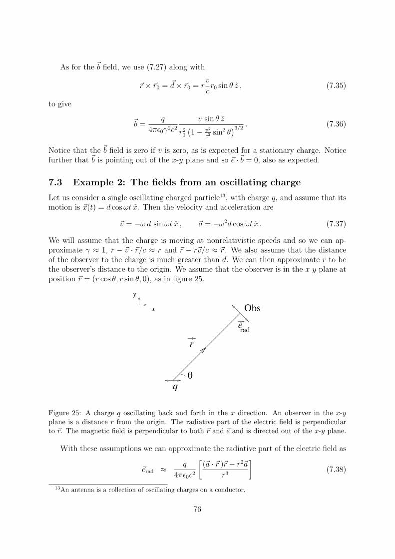
As for the ~b field, we use (7.27) along with

~r × ~r0 = ~d× ~r0 = rv

cr0 sin θ z , (7.35)

to give

~b =q

4πε0γ2c2

v sin θ z

r20

(1− v2

c2sin2 θ

)3/2. (7.36)

Notice that the ~b field is zero if v is zero, as is expected for a stationary charge. Noticefurther that ~b is pointing out of the x-y plane and so ~e ·~b = 0, also as expected.

7.3 Example 2: The fields from an oscillating charge

Let us consider a single oscillating charged particle13, with charge q, and assume that itsmotion is ~x(t) = d cosωt x. Then the velocity and acceleration are

~v = −ω d sinωt x , ~a = −ω2d cosωt x . (7.37)

We will assume that the charge is moving at nonrelativistic speeds and so we can ap-proximate γ ≈ 1, r − ~v · ~r/c ≈ r and ~r − r~v/c ≈ ~r. We also assume that the distanceof the observer to the charge is much greater than d. We can then approximate r to bethe observer’s distance to the origin. We assume that the observer is in the x-y plane atposition ~r = (r cos θ, r sin θ, 0), as in figure 25.

x

!

r

q

Obserad

y

Figure 25: A charge q oscillating back and forth in the x direction. An observer in the x-yplane is a distance r from the origin. The radiative part of the electric field is perpendicularto ~r. The magnetic field is perpendicular to both ~r and ~e and is directed out of the x-y plane.

With these assumptions we can approximate the radiative part of the electric field as

~erad ≈q

4πε0c2

[(~a · ~r )~r − r2~a

r3

](7.38)

13An antenna is a collection of oscillating charges on a conductor.

76

We should use the retarded value for ~a, which for the observer’s time t is

~a = −ω2d cosω(t− r/c) x = −ω2d cos(ωt− ~k · ~r ) x , (7.39)

where ~k is directed along r and |~k| = ω/c. Thus, we have

~erad ≈qω2d

4πε0c2

sin θ

rcos(ωt− ~k · ~r ) (sin θ x− cos θ y) . (7.40)

The term in the last parentheses is a unit vector that is orthogonal to ~r, so clearly~r · ~erad = 0. Observe that there is also an overall factor of sin θ. Hence the field iszero along the direction of the acceleration and is largest when it is orthogonal to theacceleration. The magnetic field is

~brad =1

rc~r × ~erad = − qω2d

4πε0c3

sin θ

rcos(ωt− ~k · ~r ) z . (7.41)

Let’s now compare ~erad to the dominant part of ~enr, which for this nonrelativisticlimit is the field we would find if the particle were at rest,

~enr ≈q

4πε0

~r

r3(7.42)

If θ = π/2, then |~erad| >> |~enr| if

r >>c2

ω2d=

λ2

4π2d. (7.43)

where λ is the wavelength of the radiation. Hence the radiation term dominates whenr is much greater than λ2/d, although this bound is itself much greater than λ in thenonrelativistic case where λ >> d.

7.4 The energy density of the electromagnetic field

Recall that energy is part of the momentum 4-vector pµ = (E/c, ~p ). Recall further thatcharge density ρ is part of the current density 4-vector jµ = (ρ c,~j ). One can then askwhat tensor the energy density should belong to. Since electric charge is a scalar andits current has one index, one would suspect that since pµ already comes with an index,the corresponding current density should have two indices. We write this tensor T µν andcall it the energy-momentum tensor. It is also called the stress tensor.

Let us make a list of the various components of T µν .

• The energy density is the T 00 component.

• c T 0i is the energy current density in the ith direction, in other words, it is the rateper unit area that energy is flowing in direction i. We will also call this the energyflux. Note that this has the dimensions of a power per unit area.

77

• T i0/c is the density of the ith component of momentum. However, it turns outthat T i0 = T 0i. Roughly speaking, this is because if there is a momentum density,then energy must be flowing in that direction because whatever it is that has themomentum is moving and it is taking its energy with it.

• T ij is the current density for the ith component of momentum in direction j, whichis the same as the current density for the jth component of momentum in directioni and so T ij = T ji.

Hence, T µν is a symmetric tensor, and remains symmetric in all frames.Let us now try to construct a symmetric

(20

)tensor out of a combination of Eµν

tensors. We first claim that T µν should be quadratic in Eµν . To see this, we note thatthe fields are linear in the charges, as can be seen from Maxwell equations or the explicitexpressions in (7.24) and (7.27). Therefore, the Lorentz force between two particles isproportional to the product of their charges, and so then is the work required to moveone particle toward the other one. The work done on the system changes the energydensity of the electromagnetic field. Since it is proportional to a product of charges, theenergy density must be coming from a product of electromagnetic fields.

The most general symmetric tensor quadratic in Eµν that we can write down is

T µν = aEµλEλν + b ηµνEρλEλρ . (7.44)

Lowering one index this becomes

T µν = aEµλEλν + b ηµνEρλEρλ . (7.45)

Conservation of energy and momentum leads to a current conservation law for the energymomentum tensor

∂µTµν = 0 . (7.46)

Using the field equations in empty space, ∂µEµν = 0, we find

∂µTµν = a ∂µ(Eµλ)Eλν + aEµλ∂µEλν + b ∂ν(E

ρλEρλ)

= 0 + aEµλ∂µEλν + 2bEµλ∂νEµλ ⇐ Relabel dummy index ρ→ µ

= Eµλ(a ∂µEλν − 2b ∂µEλν − 2b ∂λEνµ) ⇐ Bianchi identity (6.26)

= Eµλ(a ∂µEλν − 2b ∂µEλν − 2b ∂µEλν) ⇐ Relabel µ↔ λ and switch order

= Eµλ(a ∂µEλν − 4b ∂µEλν) . (7.47)

Hence, we find that current conservation in (7.46) requires that b = a/4. It turns outthat a = ε0, which we will show shortly.

For now, let us see what the various components are in terms of ~e and ~b. Using (6.43)for the invariant, we already see that

T µν = ε0

(EµλEλ

ν − 12ηµν(~e 2 − c2~b 2)

). (7.48)

78

The energy density T 00 is then

T 00 = ε0

(E0iEi

0 − 12η00(~e 2 − c2~b 2)

)= ε0

(3∑i=1

(−ei)(−ei)− 12(~e 2 − c2~b 2)

)=

ε02

(~e 2 + c2~b 2) . (7.49)

The energy flux components c T 0i are

c T 0i = ε0 c(E0jEj

i − 12η0i(~e 2 − c2~b 2)

)= ε0 c

(3∑

j,k=1

(−ej)(εjikc bk)− 0

)

= ε0 c2

3∑j,k=1

(εijkej bk

= ε0 c2(~e×~b )i ≡ Si . (7.50)

The vector ~S is called the Poynting vector and it “points” in the direction of the energyflux. Since the flux comes from a cross product of the ~e and ~b fields, ~S is orthogonal toboth.

We now justify the choice a = ε0. Suppose we have a large charge Q that is evenlydistributed on a shell of radius R. In this case, the electric field satisfies

~e =Q

4πε0

~r

r3r > R

~e = 0 r ≤ R . (7.51)

The energy density coming from the electric field according to (7.49) is

T 00 =Q2a

32π2ε20r4

r > R

T 00 = 0 r ≤ R , (7.52)

where we have left a unevaluated. Therefore, the energy is

E =

∫d3xT 00 =

∫ ∞R

r2dr

∫ π

0

sin θdθ

∫ 2π

0

dφQ2a

32π2ε20r4

=4πQ2a

32π2ε20

∫ ∞R

dr

r2=

Q2a

8πε20R. (7.53)

If we add a small bit of charge δQ then the energy becomes

E =(Q+ δQ)2a

8πε20R≈ Q2a

8πε20R+QδQa

4πε20R. (7.54)

79

Now let us think a little differently about adding δQ to Q. Let us start with the chargeδQ out at infinity. As we bring it toward the shell there is a Lorentz force on the chargeδQ from the ~e field in (7.51). Using (6.50) we have

~f =QδQ

4πε0

~r

r3r > R . (7.55)

Therefore, the work done on bringing the charge δQ in from infinity to the surface of theshell at r = R is

W =

∫ ∞R

drQδQ

4πε0r2=

QδQ

4πε0R. (7.56)

The work done should equal the increase in the energy of the electromagnetic field.Comparing the work done with (7.54), we see that a = ε0.

7.5 Energy flux from a moving charge

Let us now find the energy flux (Poynting vector) ~S for a moving charge. In this casewe have

~S = ε0 c2 ~e×~b = ε0 c

2 ~e×(

1

rc(~r × ~e )

). (7.57)

Using the identity ~A× ( ~B × ~C ) = ( ~A · ~C ) ~B − ( ~A · ~B )~C we have

~S = ε0 c (~e · ~e ) r − (~e · r)~e . (7.58)

In particular, for large enough r where the radiative piece will dominate, ~S reduces to

~S = ε0 c (~erad · ~erad ) r (7.59)

since r · ~erad = 0. Notice that ~S is directed outward along ~r (the coefficient in front of ris nonnegative.)

Let us now apply this to the case of the oscillating charge. Again we assume that thecharge’s motion is nonrelativisitic so we can use the results in (7.40) and (7.41) for the

fields. In this case the energy flux ~S is

~S = ε0 c (~erad · ~erad ) r

=q2ω4d2

16π2ε0c3

sin2 θ

r2cos2(ωt− ~k · ~r ) r . (7.60)

To find the total power radiated, we integrate ~S over the surface of a sphere of radius r.Doing this we get

P =

∫ π

0

sin θdθ

∫ 2π

0

dφ r2 r · ~S =

∫ π

0

sin3 θdθq2ω4d2

8πε0c3cos2(ωt− ~k · ~r )

=q2ω4d2

6πε0c3cos2(ωt− ~k · ~r ) (7.61)

80

One can consider the averaged power P over one oscillation cycle, in which case wereplace cos2(ωt− ~k · ~r ) with 1

2. Hence, this gives

P =q2ω4d2

12πε0c3. (7.62)

We can also translate this into an energy per oscillation, given by

T P =2π

ωP =

q2ω3d2

6ε0c3(7.63)

where T is the time for one oscillation. The power is emitted in the form of electromag-netic radiation and this energy is sourced by the oscillating charge. Hence, if no furtherenergy is put into the system the oscillating charge will lose energy.

Notice that the nonradiating piece does not lead to energy loss, since the nonrela-tivistic ~enr is directed along ~r and so its contribution to ~S in (7.60) is orthogonal to r.

Therefore, it cannot contribute to r · ~S.One can also derive a compact expression for the rate that power is radiated for a

general accelerating nonrelativistic charged particle. In this nonrelativistic limit, theradiative part in (7.24) is

~erad =q

4πε0c2

[(~a · ~r )~r − r2~a

r3

](7.64)

In this case, the Poynting vector is

~S =q2

16π2ε0c3

[r2(~a · ~a )− (~a · ~r )2

r4

]r . (7.65)

The power radiated, P , is then found by integrating ~S over a sphere of radius r. Withoutany loss of generality, we can choose the polar angle on the sphere to be the angle awayfrom the direction of ~a. Therefore, P is given by

P =

∫ π

0

sin θdθ

∫ 2π

0

dφ r2 r · ~S =q2

16π2ε0c3(1− cos2 θ) [~a · ~a ]

=q2

8πε0c3

(2− 2

3

)[~a · ~a ]

=q2

6πε0c3[~a · ~a ] . (7.66)

One can readily check that substituting the acceleration of an oscillating charge in (7.66)gives (7.62).

7.6 Radiation from a highly relativistic particle on a ring

As we have previously mentioned, the LHC is a particle collider with two opposing beamsof 3.5 TeV protons (eventually it will be 7 TeV protons.). The protons themselves are

81

made up of quarks and gluons, and it is actually the collisions between these constituentsthat will produce new particles, perhaps with masses up to a 1 TeV. However, it will notbe easy to observe these new particles. The problem is that all the other constituents ofthe protons are still there, so the signature of the collision is a big mess and it will takea tremendous effort to extract the interesting information.

In fact, the 27 km LHC tunnel was built for a previous experiment, the Large ElectronPositron collider, otherwise known as LEP. In the final version of this experiment theelectrons and positrons each had over 80 GeV of energy. The nice thing about anelectron-positron collider is that these particles are point particles which means theyare not made up of anything else (or at least not at the scales that we can see). Thuswhen they collide, their signal is very clean. Furthermore, all of the energy is availableto make particles. So you might be asking, why did they not just increase the energiesof the electron-positron collider so that each particle had 500 GeV in order to createparticles with 1 TeV of rest energy? We now show that it is because of energy loss dueto radiation. This radiation is known as synchrotron radiation.

We are just interested in the radiation term, so we can use equation (7.59) for ~S. Weassume that the particle is moving at constant speed around a ring of radius R. Thevelocity vector ~v points along the ring and the acceleration ~a points toward the centerof the ring. Taking the result from (7.24), we find

~S = ε0 c (~erad · ~erad ) r

=q2

16π2ε0c3

[((~a · ~r )(~r − r~v/c)− r(r − ~v · ~r/c)~a) · ((~a · ~r )(~r − r~v/c)− r(r − ~v · ~r/c)~a)

(r − ~v · ~r/c)6

]r

=q2

16π2ε0c3

[r2(r − ~v · ~r/c)2~a · ~a− 2r(r − ~v · ~r/c)(~a · ~r )2 + (r2 − 2r~v · ~r + r2v2/c2)(~a · ~r )2

(r − ~v · ~r/c)6

]r

=q2

16π2ε0c3

[r2(r − ~v · ~r/c)2~a · ~a− r2(1− v2/c2)(~a · ~r )2

(r − ~v · ~r/c)6

]r

=q2

16π2ε0c3

[r2~a · ~a

(r − ~v · ~r/c)4− r2(~a · ~r )2/γ2

(r − ~v · ~r/c)6

]r (7.67)

where we used that ~v · ~a = 0. Observe that the flux is greatest along the direction of ~vbecause of the denominators. In fact if ~r is parallel to ~v then ~a · ~r = 0 so only the firstterm contributes.

Suppose we compute the energy emitted by the charged particle as it travels a lengthd around the ring, where d << R. The space-time point at the beginning of thistrajectory is labeled P and the point at the end is Q. Over such a short distance, theparticle’s trajectory is well approximated by a straight line. To find the energy emitted,we assume that we have a large sphere of radius r around the center of the particle’strajectory and we integrate the power through this sphere over the time from when theradiation emitted at P arrives to when the radiation emitted at Q arrives. There is asubtlety that needs to be taken into account and which is described in figure 26 (a). Thefigure shows the simultaneous circular wave-fronts from the radiation emitted at P andQ. Since the radiation is emitted at P before Q, the wave-front from P is larger. Asis clear from the diagram, the time between the arrival of the P wave-front and the Q

82

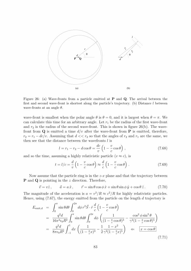
l

!dP Q

(a)

d

!

r

(b)

rr12

Figure 26: (a) Wave-fronts from a particle emitted at P and Q. The arrival between thefirst and second wave-front is shortest along the particle’s trajectory. (b) Distance l betweenwave-fronts at an angle θ.

wave-front is smallest when the polar angle θ is θ = 0, and it is largest when θ = π. Wecan calculate this time for an arbitrary angle. Let r1 be the radius of the first wave-frontand r2 is the radius of the second wave-front. This is shown in figure 26(b). The wave-front from Q is emitted a time d/v after the wave-front from P is emitted, therefore,r2 = r1 − dc/v. Assuming that d << r2 so that the angles of r2 and r1 are the same, wethen see that the distance between the wavefronts l is

l = r1 − r2 − d cos θ =dc

v

(1− v

ccos θ

), (7.68)

and so the time, assuming a highly relativistic particle (v ≈ c), is

t = l/c =d

v

(1− v

ccos θ

)≈ d

c

(1− v

ccos θ

). (7.69)

Now assume that the particle ring is in the z-x plane and that the trajectory betweenP and Q is pointing in the z direction. Therefore,

~v = vz , ~a = a x , ~r = sin θ cosφ x+ sin θ sinφ y + cos θ z . (7.70)

The magnitude of the acceleration is a = v2/R ≈ c2/R for highly relativistic particles.Hence, using (7.67), the energy emitted from the particle on the length d trajectory is

Eemit,d =

∫ π

0

sin θdθ

∫ 2π

0

dφ r2~S · r dc

(1− v

ccos θ

)=

q2d

16π2ε0R2

∫ π

0

sin θdθ

∫ 2π

0

dφ

(1

(1− vc

cos θ)3− cos2 φ sin2 θ

γ2(1− vc

cos θ)5

)=

q2d

8πε0R2

∫ 1

−1

dx

(1

(1− vcx)3− 1

2

1− x2

γ2(1− vcx)5

)⇐ x = cos θ

(7.71)

83

This integral is dominated near x = 1, but its evaluation is slightly tricky. If we write

1− x2 =

(1− c2

v2

)+ 2

c2

v2

(1− v

cx)− c2

v2

(1− v

cx)2

, (7.72)

and keep only the contribution from the x = 1 boundary, we get

Eemit,d ≈q2d

8πε0R2

(c

2v

1

(1− v/c)2− 1

2γ2

(c

4v

1− c2/v2

(1− v/c)4+

2c3

3v3

1

(1− v/c)3+ . . .

))≈ q2d

8πε0R2

(1

2

1

(1− v/c)2− 1

2γ2

(1

4

(−2)

(1− v/c)3+

2

3

1

(1− v/c)3

)), (7.73)

where the dots indicate a term that is subdominant so it is dropped. In the last step, wesubstitute v for c wherever it does not lead to a singularity. We can improve this somemore but approximating γ2 as

γ2 =1

1− v2/c2=

1

(1 + v/c)(1− v/c)≈ 1

2(1− v/c). (7.74)

This leads to

Eemit,d ≈q2d

8πε0R2

(1

2+

1

2− 2

3

)1

(1− v/c)2

≈ q2d γ4

6πε0R2. (7.75)

To find the power emitted, P , we simply divide Eemit,d by the time it takes the particleto move a distance d, d/c. This gives

P =q2c γ4

6πε0R2. (7.76)

To instead get the energy emitted for one complete revolution, we only need to replaced with 2πR, the circumference of the ring. This then gives our final result

Eemit/revolution ≈ q2 γ4

3 ε0R. (7.77)

Note in particular the γ4 term. This means that lighter particles will radiate more thanheavier ones when their kinetic energies are the same.

Let us now plug in some numbers to see the size of the effect. The radius of theLHC tunnel is 4.3 km. If we consider 7 TeV protons, then γ ≈ 7500. Hence for everyrevolution, a single proton will radiate

Eproton ≈(1.6× 10−19 coul)2(7500)4

3(8.85× 10−12 F/m)(4.3× 103 m)

= 7.6× 10−16 joules = 4800 eV . (7.78)

84

Hence, the proton gives up a very small percentage of its energy to radiation. Nextconsider an 80 GeV electron at LEP. In this case γ ≈ 1.6× 105 and so the radiation lossper turn is

Eelectron ≈(1.6× 10−19 coul)2(1.6× 105)4

3(8.85× 10−12 F/m)(4.3× 103 m)

= 1.5× 10−10 joules = 0.9 GeV . (7.79)

Hence, the electron is radiating one per cent of its energy per turn. Energy has to besupplied to the electrons for each revolution in order to compensate for their radiationloss. This can lead to a huge power consumption.

We now see what we are in store for if we try to have 500 GeV electrons in the LHCtunnel. In this case γ ≈ 106 and the radiation loss would be 1.5 TeV per revolution,three times the kinetic energy of the electron! As you might imagine, it is not practicalto compensate for such a huge loss. Hence, it is better to go with protons.

7.7 Radiation from a highly relativistic particle on a ring, donedifferently (and quickly)

In this section we give a quick and dirty way of obtaining the result in the previoussection. The idea is the following. In the instantaneous rest frame of the acceleratingparticle the power radiated can be computed using the nonrelativistic result in (7.66).The acceleration in the instantaneous rest frame is the proper acceleration ~α whichsatisfies αναν = −~α · ~α. For the particle going around the circle, γ is not changing, andso from (7.20) we have that ~α · ~α = γ4~a · ~a. Thus, the power radiated in the chargedparticle’s frame, P ′, is

P ′ =q2cγ4

6πε0R2. (7.80)

Going back to the lab frame we have

P =dE

dt=γ dE ′

γ dt′= P ′ , (7.81)

matching (7.76). One factor of γ in (7.81) comes from time dilation, dt = γ dt′. Theother factor comes from Lorentz transforming the radiation’s energy. The differentialdE ′ is part of a 4-vector dpµ

′. In the charged particle’s rest frame we can see from (7.65)

that the radiation is symmetric about the forward and backward direction since ~α isorthogonal to the boost direction. Hence the 4-vector has the form dpµ

′= (dE ′/c, d~p

′

⊥),where d~p

′

⊥ · ~v = 0. Therefore the boost direction is orthogonal to d~p′

⊥ and so we havedpµ = (γdE ′/c, d~p

′

⊥), from which it follows that dE = γ dE ′.

85

8 Special relativity and analytic mechanics

In this section we combine special relativity with what you have learned in the analyticmechanics part of the course.

8.1 The free relativistic particle

Suppose we have a free nonrelativistic particle with mass m. The Lagrangian for thissystem is given by

L = 12m~x · ~x , (8.1)

and the action is

S =

∫Ldt =

∫12m~x · ~x dt . (8.2)

Let us now consider the relativistic generalization of (8.1). We want to have trans-lation invariance in 3 + 1 space-time dimensions as well as Lorentz invariance. Thislast statement means that the Lagrangian should be a Lorentz invariant. The obviousgeneralization appears to be

L = C mdxµ

dτ

dxν

dτηµν = −m dxµ

dτ

dxµdτ

= −mxµxµ , (8.3)

where C is a constant which we set to C = −1 (to be justified later). The action is then

S = −∫

mxµxµ dτ . (8.4)

But recall from earlier sections that the differentials are constrained by dxµdxµ = c2dτ 2

and so the Lagrangian in (8.3) is actually a constant,

L = −mc2 , (8.5)

and the action is

S = −∫mc2dτ . (8.6)

Hence, the action is the negative rest energy multiplied by the elapsed proper time alongthe particle’s world-line. By minimizing the action one finds the path that maximizes theproper time. Recall that when we discussed the twin paradox, the twin which took thestraight path had a larger proper time than the twin who took a path that had a changein velocity along its world-line, so a maximization of the proper time seems reasonablefrom this perspective.

Substituting c2dτ 2 = dxµdxµ, the action can be rewritten as

S = −∫mc√dxµdxµ = −

∫mc

√∂xµ

∂λ

∂xµ∂λ

dλ , (8.7)

86

where λ can be any variable that parameterizes the path of the particle. The Lagrangianis now written as

L = −mc√∂xµ

∂λ

∂xµ∂λ

, (8.8)

and the equations of motion are given by

d

dλ

(∂L

∂xµ

)− ∂L

∂xµ= 0

− d

dλ

(mc

xµ√xν xν

)= 0 , (8.9)

where xµ = ∂xµ

∂λ. If we let λ = τ then

√xν xν = c and the equations of motion become

− d

dτ(mxµ) = 0 . (8.10)

mxµ = pµ is the 4-momentum we discussed in previous sections, and so the equations ofmotion indicate that it is constant in proper time.

The freedom to choose any variable for λ is known as reparameterization invarianceand will lead us to a surprising result (perhaps) when we construct a Hamiltonian. Recallhow one constructs the canonical momentum and Hamiltonian from the Lagrangian. Thecanonical momentum conjugate to a coordinate is found by varying the Lagrangian withrespect to its time derivative. In this case λ is playing the role of time, hence we have

rµ =∂L

∂xµ= −mc xµ√

xν xν. (8.11)

and we use rµ to distinguish the canonical momentum associated with λ from the 4-momentum pµ above. If we were to let λ = τ then we would have rµ = −pµ. TheHamiltonian is given by

H = rµxµ − L (8.12)

and the equations of motion for the coordinate xµ and the canonical momentum rµ arefound from the Poisson brackets,

xµ = {xµ, H} ≡(∂xµ

∂xν∂H

∂rν− ∂xµ

∂rν

∂H

∂xν

)rµ = {pµ, H} ≡

(∂rµ∂xν

∂H

∂rν− ∂rµ∂rν

∂H

∂xν

). (8.13)

However, in our case the Hamiltonian is given by

H = xµrµ − L = −mc xµxµ√xν xν

+mc√xν xν = 0 , (8.14)

in other words, H is constrained to be 0. Why do we get this contraint? Remember thatin the usual nonrelativistic case the Hamiltonian is used to generate the time evolution

87

of the coordinates and momenta through the Poisson brackets. In the case here, H isgenerating a reparameterization of λ. Since the theory is reparameterization invariant,we can change to a new value of λ and leave the values for xµ and pµ unchanged. HavingH = 0 means that xµ and rµ stay fixed under the reparameterization.

Even though we have a trivial H, we have an extra conjugate momentum, r0, as com-pared to the nonrelativistic case. However, it is possible to get a nontrivial Hamiltonianby choosing a parameterization for λ that evolves in time. To this end we let λ = t, thetime coordinate in frame S. For this choice the action becomes

S = −∫mc

√c2 − ∂~x

∂t· ∂~x∂t

dt , (8.15)

and we see that x0 is no longer a coordinate to be varied in the action and so there isone less conjugate momentum. The canonical momenta for the spatial coordinates withrespect to t is

ri =∂L

∂ ∂xi

∂t

= mc∂xi

∂t√c2 − ∂~x

∂t· ∂~x∂t

= m∂xi

∂t√1− 1

c2∂~x∂t· ∂~x∂t

. (8.16)

This can be inverted using

~r · ~r = m2∂~x∂t· ∂~x∂t

1− 1c2∂~x∂t· ∂~x∂t

⇒ 1

c2

∂~x

∂t· ∂~x∂t

=~r · ~r

m2c2 + ~r · ~r(8.17)

which then gives

∂~x

∂t=

~r√m2 + ~r · ~r/c2

. (8.18)

Note also that using ~v = ∂~x∂t

the momentum is

~r = mγ ~v , (8.19)

which is the anticipated form if ~r is the spatial part of the 4-momentum.The Hamiltonian is then

H =∂xi

∂tri − L =

mc2√1− 1

c2∂~x∂t· ∂~x∂t

=√m2c4 + ~r · ~r c2 . (8.20)

H now has the expected form of the energy in frame S, since ~r is the spatial part of the4-momentum. In terms of ~r and H we have that pµ = (H,−~r).

The Hamiltonian now evolves xi in time t, hence we have

∂xi

∂t= {xi, H} =

~r√m2c2 + ~r · ~r

= ~v

∂ri∂t

= {ri, H} = 0 . (8.21)

88

These are the expected equations of motion. Of course, we are free to choose λ to bethe time coordinate for any inertial frame, and since dxµdxµ is a Lorentz invariant, wewould find similar equations for any inertial frame we choose.

To close this subsection, we note that if ∂~x∂t· ∂~x∂t<< c2, then the action in (8.15) is

approximately

S ≈∫ (−mc2 + 1

2m∂~x

∂t· ∂~x∂t

)dt . (8.22)

The first term in the parentheses is a constant and does not affect the equations ofmotion. The second term is the usual nonrelativistic Lagrangian. Hence, this justifiesthe above choice C = −1.

8.2 Coupling to an external field

We now consider the case where the particle has charge q and is in the presence of anelectromagnetic field. The action should be Lorentz invariant and also invariant undergauge transformations. The appropriate action is

S = −∫mc2 dτ − 1

c

∫q Aµdx

µ . (8.23)

which is clearly Lorentz invariant. The second integral is a line integral along the parti-cle’s world-line. Under a gauge transformation it transforms to

−1

c

∫q Aµdx

µ − 1

c

∫q ∂µΦdxµ . (8.24)

The second term in (8.24) is a total derivative and hence cannot affect the equations ofmotion. Therefore, the equations of motion are invariant under gauge transformations.

Expressing Aµ in terms of the potentials, Aµ = (ϕ,−c ~w ), the second integral can bewritten as

−1

c

∫q Aµdx

µ = −1

c

∫q Aµ

∂xµ

∂tdt = −

∫q

(ϕ− ~w · ∂~x

∂t

)dt . (8.25)

The equations of motion are then found to be

0 =d

dt

(∂L

∂ ∂xi

∂t

)− ∂L

∂xi

=d

dt

m ∂xi

∂t√1− 1

c2∂~x∂t· ∂~x∂t

+ qwi

+ q∂ϕ

∂xi− q∂wj

∂xi∂xj

∂t(8.26)

Hence, using the expressions for ~e and ~b in (7.1), this becomes

dpi

dt= f i = −q

(∂ϕ

∂xi+∂wi∂t

)− q∂x

j

∂t

∂wi∂xj

+ q∂wj

∂xi∂xj

∂t

= q ei + q εijk vj bk

~f = q(~e+ ~v ×~b) , (8.27)

89

which is the Lorentz force equation.Note that the ~p that appears here is not the canonical momentum. Instead, this is

given by

ri =∂L

∂ ∂xi

∂t

= pi + q wi . (8.28)

Therefore, one finds the Hamiltonian

H = ri∂xi

∂t− L = pi

∂xi

∂t+ q φ

=√m2c4 + (~r − q ~w) · (~r − q ~w)c2 + q φ (8.29)

where we essentially replaced ~r with ~r − q ~w in (8.20) and added the contribution fromthe electric potential.

8.3 Symmetries and constants of the motion for the free parti-cle system

Let us return to the case of the nonrelativistic free particle. The Lagrangian and theaction in (8.1) and (8.2) have some symmetries. First, they are invariant under constantshifts in ~x,

~x(t)→ ~x(t) + ~x0 . (8.30)

Notice that if the Lagrangian had had a potential term,

L = 12m~x · ~x− V (~x) , (8.31)

then in general L would not be invariant under the shift in (8.30).We now show that this invariance leads to a conservation law. Suppose we consider

an infinitesimal shift, ~x→ ~x+ ~ε. Then the change in the Lagrangian is

δL = 0 =∂L

∂~x· ddtδ~x+

∂L

∂~x· δ~x

=d

dt

(∂L

∂~x· ~ε)−(d

dt

(∂L

∂~x

)− ∂L

∂~x

)· ~ε , (8.32)

where we assumed that the change of L is zero because of the invariance. The secondterm on the second line of (8.32) is zero by the equations of motion, hence if we use that~ε is independent of t then we find the conservation law

d

dt

∂L

∂~x=

d

dtm~x =

d

dt~p = 0 . (8.33)

Hence, the translation invariance leads to a conservation equation, in this case conser-vation of the three-momentum.

90

The Lagrangian in (8.1) is also invariant under the three-dimensional rotations, xi →Ri

j xj, where Ri

j is a three-dimensional rotation matrix and where the components i, j,run from 1 to 3. If we assume that the rotation is very small then we can write Ri

j as

Rij = δij + i εa Ta

ij , a = 1 . . . 3 , (8.34)

where the εa are three independent infinitesimal angles that define the rotation, and theTa are matrices that “generate” the rotation. The repeated a index in (8.34) is summedover. A useful choice for the independent rotations are rotations in the y − z, z − x andx− y planes, in which case we would have

T1 =

0 0 00 0 i0 −i 0

, T2 =

0 0 −i0 0 0i 0 0

, T3 =

0 i 0−i 0 00 0 0

. (8.35)

Notice that the components of the Ta can be written as

Taij = i εaij , (8.36)

where εaij is the completely antisymmetric tensor in three spatial directions,

εaij = −εiaj = −εjia, ε123 = 1 . (8.37)

With the definition in (8.34), the transformation on the components of ~x are

xi → xi + δxi = xi + i εaTaij x

j . (8.38)

Repeating the exercise in (8.32) we find

δL = 0 =∂L

∂~x· ddtδ~x+

∂L

∂~x· δ~x

=d

dt

(∂L

∂xi(i Ta

ij)x

j

)εa −

(d

dt

(∂L

∂~x

)− ∂L

∂~x

)· ~δx , (8.39)

Again using the equations of motion and assuming that εa is constant in t, we find that

La ≡ εaijxipj (8.40)

are constants of the motion. These are simply the components of the angular momentumvector

~L = ~x× ~p . (8.41)

In both the cases of translations and rotations, we have a continuous symmetry whichallows us to construct a set of conserved quantities. In fact for any continuous symmetryof the Lagrangian we could have constructed a conserved quantity. This observation isknown as Noether’s theorem.

91

Turning now to the relativistic case, the translation symmetry of the action in (8.7)is very similar to the translation symmetry in (8.2) and leads to the conserved quantities

d

dλ

∂L

∂xµ=

d

dλrµ = 0 . (8.42)

If we let λ = τ then rµ = −pµ and the four dimensional space-time translation symmetryleads to conservation of the 4-momentum, d

dτpµ = 0, which includes a component for

conservation of energy.The invariance under Lorentz translations leads to a new set of conserved quantities.

Recall that a Lorentz transformation relates the coordinates in frame S of a space-timepoint to the coordinates in S′ for the same space-time point by

(xµ′ − xµ′) = Λµ′

ν(xν − xν) , (8.43)

where xµ is a reference point so that the relation is between displacements. From nowon we choose the reference point to be at the origin where xµ = 0. Instead of changingthe reference frame we want to change the the space-time point so that the coordinatesof the new point in S are the same as if we had kept the point the same and boosted toS′. Hence the transformation of the space-time point is

xµ → Λµνx

ν . (8.44)

Notice that both indices on Λ are unprimed. For an infinitesimal transformation wewould have

xµ → xµ + i 12εσρMσρ

µνx

ν , (8.45)

where εσρ is an infinitesimal angle or rapidity in the 3 + 1 dimensional space-time, whichsatisfies εσρ = −ερσ. For example, the {01} component would correspond to an infinites-imal rapidity from boosting in the x direction. The generators Mσρ are given by

M01 =

0 i 0 0i 0 0 00 0 0 00 0 0 0

M02 =

0 0 i 00 0 0 0i 0 0 00 0 0 0

M03 =

0 0 0 i0 0 0 00 0 0 0i 0 0 0

M12 =

0 0 0 00 0 i 00 −i 0 00 0 0 0

M23 =

0 0 0 00 0 0 00 0 0 i0 0 −i 0

M31 =

0 0 0 00 0 0 −i0 0 0 00 i 0 0

(8.46)

In terms of the components we can write each of these as

Mσρµν = −Mρσ

µν = i(ησνδ

µρ − ηρνδµσ) . (8.47)

If we lower the µ index this takes the more symmetric form

Mσρµν = i(ησνηρµ − ησµηρν) . (8.48)

92

The Lagrangian is invariant under the transformation in (8.45), hence we are led to

δL = 0 =∂L

∂xµd

dλδxµ +

∂L

∂xµδxµ

=d

dλ

(∂L

∂xµ( i

2Mσρ

µν)x

νεσρ)−(d

dλ

(∂L

∂xµ

)− ∂L

∂xµ

)δxµ . (8.49)

Therefore, Θσρ is a constant of the motion, where

Θσρ = iMσρµνrµxν = −xσrρ + xρrσ . (8.50)

If we now let λ = τ then this becomes

Θσρ = xσpρ − xρpσ . (8.51)

Θσρ is an antisymmetric(

02

)tensor and is the generalization of the angular-momentum

vector. In fact, we can see that Θij = −εijkLk.

93