job_talk_2014-01-13_final
75
-
Upload
hector-flores -
Category
Documents
-
view
1 -
download
0
Transcript of job_talk_2014-01-13_final

Exam Schools, Ability, and the E�ects ofA�rmative Action: Latent Factor Extrapolation in
the Regression Discontinuity Design
Miikka Rokkanen
Massachusetts Institute of Technology

Introduction
Latent Factor Modeling in a Sharp RD Design
Boston Exam Schools
Identi�cation and Estimation
Extrapolation Results
Counterfactual Simulations
Placebo Experiments
Conclusions
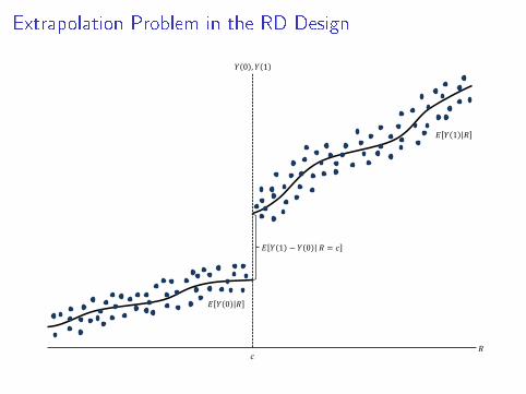
Extrapolation Problem in the RD Design
𝐸[𝑌(1) − 𝑌(0)| 𝑅 = 𝑐]
𝑅
𝐸[𝑌(1)|𝑅]
𝐸[𝑌(0)|𝑅]
𝑐
𝑌(0),𝑌(1)
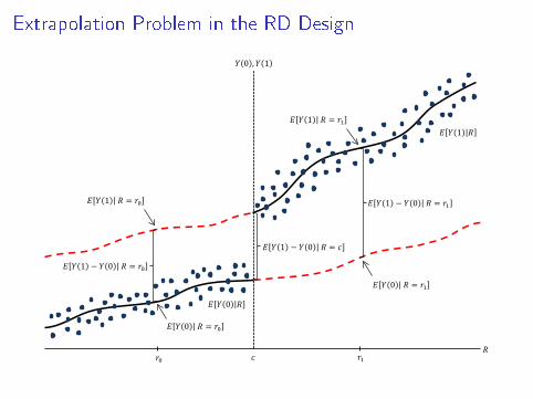
Extrapolation Problem in the RD Design
𝐸[𝑌(1) − 𝑌(0)| 𝑅 = 𝑐]
𝑅
𝐸[𝑌(1)|𝑅]
𝐸[𝑌(0)|𝑅]
𝑐
𝐸[𝑌(1) − 𝑌(0)| 𝑅 = 𝑟1]
𝑟1
𝐸[𝑌(0)| 𝑅 = 𝑟1]
𝐸[𝑌(1)| 𝑅 = 𝑟1]
𝐸[𝑌(1) − 𝑌(0)| 𝑅 = 𝑟0]
𝐸[𝑌(0)| 𝑅 = 𝑟0]
𝑟0
𝐸[𝑌(1)| 𝑅 = 𝑟0]
𝑌(0),𝑌(1)

Boston Exam Schools
I Three selective high schools that are seen as the �agship ofthe Boston public school system
I RD estimates show little evidence of e�ects for marginalapplicants (Abdulkadiroglu, Angrist & Pathak, forthcoming)
I Is the lack of e�ects generalizable for inframarginal applicants?
I Important question for discussion of a�rmative action atselective school admissions

This Paper
1. Develop a latent factor-based approach to the extrapolation oftreatment e�ects away from the cuto� in RD
I Nonparametric identi�cation of treatment e�ects at any pointin the running variable distribution
2. Estimate e�ects of Boston exam school attendance for fullpopulation of applicants
I Achievement gains concentrated among lower-scoringapplicants
3. Simulate e�ects of introducing minority/socioeconomicpreferences into exam school admissions
I Both reforms increase average achievement among a�ectedapplicants

Related Literature
1. Extrapolation of treatment e�ects in RD: Angrist &Rokkanen (2013); Cook & Wing (2013); Dong & Lewbel(2013)
2. Latent factor and measurement error models: Hu &Schennach (2008); Cunha, Heckman & Schennach (2010);Evdokimov & White (2012)
3. (Semi-)nonparametric instrumental variables models:Newey & Powell (2003); Blundell, Chen & Kristensen (2007);Darolles, Fan, Florens & Renault (2011)
4. E�ects of attending selective middle/high schools:Jackson (2010); Pop-Eleches & Urquiola (2013);Abdulkadiroglu, Angrist & Pathak (forthcoming)
5. E�ects of a�rmative action in school admissions:Arcidiacono (2005); Card & Krueger (2005); Hinrichs (2012)

Introduction
Latent Factor Modeling in a Sharp RD Design
Boston Exam Schools
Identi�cation and Estimation
Extrapolation Results
Counterfactual Simulations
Placebo Experiments
Conclusions

Latent Factor Framework
I Running variable R is a noisy measure of a latent factor θ :
R = gR (θ ,νR)
I Potential outcomes Y (0) and Y (1) depend on θ but not onthe noise in R :
(Y (0) ,Y (1))⊥⊥ R | θ
I Example: selective school admission
I R: entrance exam scoreI θ : latent abilityI Y (0), Y (1): future achievement
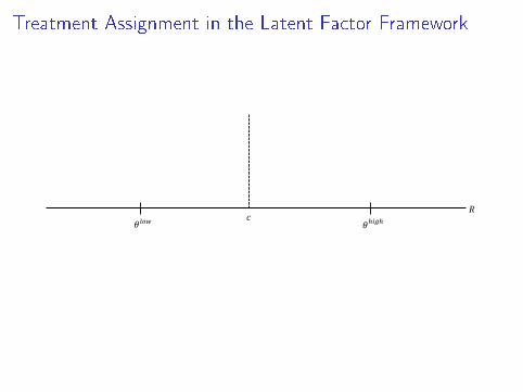
Treatment Assignment in the Latent Factor Framework
𝑅 𝜃𝑙𝑜𝑤
𝜃ℎ𝑖𝑔ℎ
𝑐
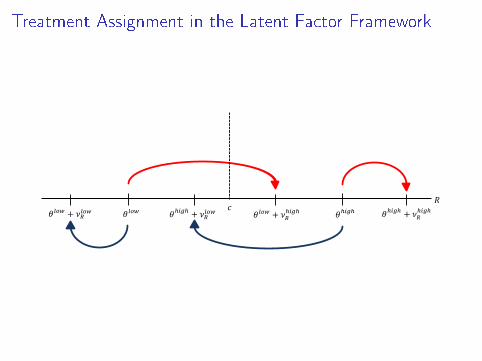
Treatment Assignment in the Latent Factor Framework
𝑅 𝜃𝑙𝑜𝑤
𝜃ℎ𝑖𝑔ℎ
𝜃𝑙𝑜𝑤 + 𝜈𝑅𝑙𝑜𝑤 𝜃𝑙𝑜𝑤 + 𝜈𝑅ℎ𝑖𝑔ℎ 𝜃ℎ𝑖𝑔ℎ + 𝜈𝑅𝑙𝑜𝑤 𝜃ℎ𝑖𝑔ℎ + 𝜈𝑅
ℎ𝑖𝑔ℎ 𝑐
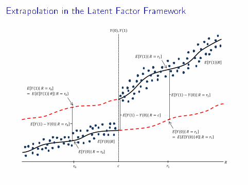
Extrapolation in the Latent Factor Framework
𝐸[𝑌(1) − 𝑌(0)| 𝑅 = 𝑐]
𝑅
𝐸[𝑌(1)|𝑅]
𝐸[𝑌(0)|𝑅]
𝑐
𝐸[𝑌(1) − 𝑌(0)| 𝑅 = 𝑟1]
𝑟1
𝐸[𝑌(0)| 𝑅 = 𝑟1]= 𝐸{𝐸[𝑌(0)| 𝜃]| 𝑅 = 𝑟1}
𝐸[𝑌(1)| 𝑅 = 𝑟1]
𝐸[𝑌(1) − 𝑌(0)| 𝑅 = 𝑟0]
𝐸[𝑌(0)| 𝑅 = 𝑟0]
𝑟0
𝐸[𝑌(1)| 𝑅 = 𝑟0]= 𝐸{𝐸[𝑌(1)| 𝜃]| 𝑅 = 𝑟0}
𝑌(0),𝑌(1)

Object 1: Conditional Latent Factor Distribution
𝜃
𝑓𝜃|𝑅(𝜃|𝑟)
𝑓𝜃|𝑅(𝜃|𝑟0)
𝑓𝜃|𝑅(𝜃|𝑟1)

Object 2: Latent Conditional Expectation Functions
𝜃
𝑌(0),𝑌(1)
𝐸[𝑌(1)|𝜃]
𝐸[𝑌(0)|𝜃]

Identi�cation Using Multiple Noisy Measures
I Suppose one has available three noisy measures of θ :
M1 = gM1(θ ,νM1
)
M2 = gM2(θ ,νM2
)
M3 = gM3(θ ,νM3
)
where M1,M2 are continuous, and M3 is potentially discrete
I R is a deterministic function of a subset of M = (M1,M2,M3)
I Example: selective school admissions
I R = M1: entrance exam scoreI M2,M3: baseline test scores
Identi�cation with less than three measures
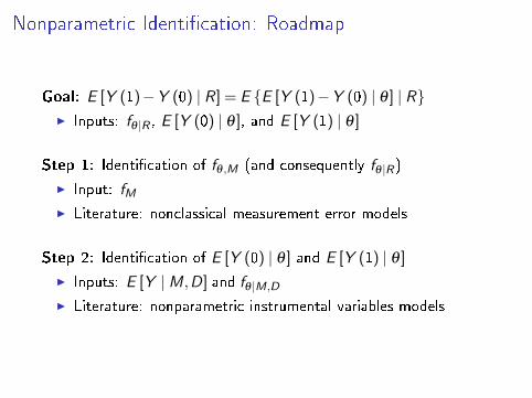
Nonparametric Identi�cation: Roadmap
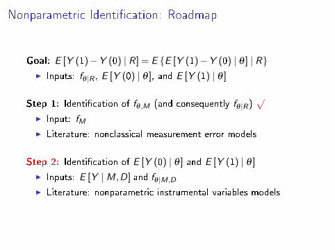
Goal: E [Y (1)−Y (0) | R] = E {E [Y (1)−Y (0) | θ ] | R}I Inputs: fθ |R , E [Y (0) | θ ], and E [Y (1) | θ ]
Step 1: Identi�cation of fθ ,M (and consequently fθ |R)
I Input: fMI Literature: nonclassical measurement error models
Step 2: Identi�cation of E [Y (0) | θ ] and E [Y (1) | θ ]
I Inputs: E [Y |M,D] and fθ |M,D
I Literature: nonparametric instrumental variables models
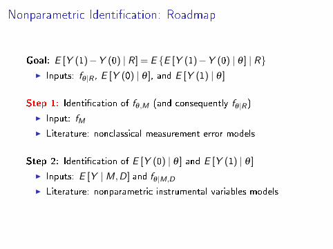
Nonparametric Identi�cation: Roadmap
Goal: E [Y (1)−Y (0) | R] = E {E [Y (1)−Y (0) | θ ] | R}I Inputs: fθ |R , E [Y (0) | θ ], and E [Y (1) | θ ]
Step 1: Identi�cation of fθ ,M (and consequently fθ |R)
I Input: fMI Literature: nonclassical measurement error models
Step 2: Identi�cation of E [Y (0) | θ ] and E [Y (1) | θ ]
I Inputs: E [Y |M,D] and fθ |M,D
I Literature: nonparametric instrumental variables models

Parametric Illustration
I Suppose the measurement model takes the form
Mk = µMk+ λMk
θ + νMk,k = 1,2,3
where µM1= 0, λM1
= 1, andθ
νM1
νM2
νM3
∼ N
µθ
000
,
σ2θ
0 0 00 σ2
νM10 0
0 0 σ2νM2
0
0 0 0 σ2νM3
I Then the unknown parameters can be obtained from themeans, variances, and covariances of M
Details
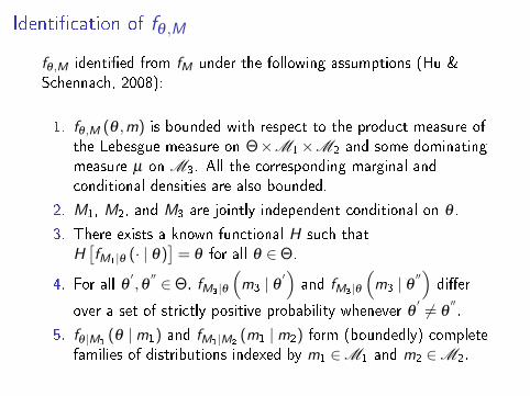
Identi�cation of fθ ,M
fθ ,M identi�ed from fM under the following assumptions (Hu &Schennach, 2008):
1. fθ ,M (θ ,m) is bounded with respect to the product measure ofthe Lebesgue measure on Θ×M1×M2 and some dominatingmeasure µ on M3. All the corresponding marginal andconditional densities are also bounded.
2. M1, M2, and M3 are jointly independent conditional on θ .
3. There exists a known functional H such thatH[fM1|θ (· | θ)
]= θ for all θ ∈Θ.
4. For all θ′,θ′′ ∈Θ, fM3|θ
(m3 | θ
′)and fM3|θ
(m3 | θ
′′)di�er
over a set of strictly positive probability whenever θ′ 6= θ
′′.
5. fθ |M1(θ |m1) and fM1|M2
(m1 |m2) form (boundedly) completefamilies of distributions indexed by m1 ∈M1 and m2 ∈M2.
Nonparametric Identi�cation: Roadmap
Goal: E [Y (1)−Y (0) | R] = E {E [Y (1)−Y (0) | θ ] | R}I Inputs: fθ |R , E [Y (0) | θ ], and E [Y (1) | θ ]
Step 1: Identi�cation of fθ ,M (and consequently fθ |R)√
I Input: fMI Literature: nonclassical measurement error models
Step 2: Identi�cation of E [Y (0) | θ ] and E [Y (1) | θ ]
I Inputs: E [Y |M,D] and fθ |M,D
I Literature: nonparametric instrumental variables models

Parametric Illustration
I Suppose the latent outcome model takes the form
E [Y (D) | θ ] = αD + βDθ , D = 0,1
and
(Y (0) ,Y (1))⊥⊥M | θ
I Then the unknown parameters can be obtained from theconditional means of Y and θ given M to the left and right ofthe cuto�
Details
Identi�cation of E [Y (0) | θ ] and E [Y (1) | θ ]
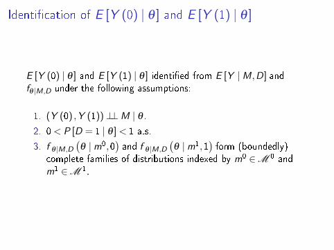
E [Y (0) | θ ] and E [Y (1) | θ ] identi�ed from E [Y |M,D] andfθ |M,D under the following assumptions:
1. (Y (0) ,Y (1))⊥⊥M | θ .2. 0< P [D = 1 | θ ] < 1 a.s.
3. f θ |M,D
(θ |m0,0
)and f θ |M,D
(θ |m1,1
)form (boundedly)
complete families of distributions indexed by m0 ∈M 0 andm1 ∈M 1.

Nonparametric Identi�cation: Roadmap
Goal: E [Y (1)−Y (0) | R] = E {E [Y (1)−Y (0) | θ ] | R}I Inputs: fθ |R , E [Y (0) | θ ], and E [Y (1) | θ ]
Step 1: Identi�cation of fθ ,M (and consequently fθ |R)√
I Input: fMI Literature: latent factor and measurement error models
Step 2: Identi�cation of E [Y (0) | θ ] and E [Y (1) | θ ]√
I Inputs: E [Y |M,D] and fθ |M,D
I Literature: nonparametric instrumental variables models

Extensions
Extension 1: Latent Factor Modeling in a Fuzzy RD Design
Extension 2: Settings with Multiple Latent Factors

Introduction
Latent Factor Modeling in a Sharp RD Design
Boston Exam Schools
Identi�cation and Estimation
Extrapolation Results
Counterfactual Simulations
Placebo Experiments
Conclusions
Boston Exam Schools
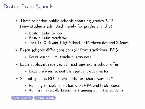
I Three selective public schools spanning grades 7-12(new students admitted mainly for grades 7 and 9)
I Boston Latin SchoolI Boston Latin AcademyI John D. O'Bryant High School of Mathematics and Science
I Exam schools di�er considerably from traditional BPS
I Peers, curriculum, teachers, resources
I Each applicant receives at most one exam school o�er
I Most preferred school the applicant quali�es for
I School-speci�c RD experiments for �sharp samples�
I Running variable: rank based on GPA and ISEE scoresI Admissions cuto�: lowest rank among admitted students
DA Algorithm Sharp Sample
Data and Sample
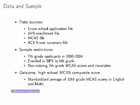
I Data sources:
I Exam school application �leI BPS enrollment �leI MCAS �leI ACS 5-year summary �le
I Sample restrictions:
I 7th grade applicants in 2000-2004I Enrolled in BPS in 6th gradeI Non-missing 4th grade MCAS scores and covariates
I Outcome: high school MCAS composite score
I Standardized average of 10th grade MCAS scores in Englishand Math
Descriptive Statistics
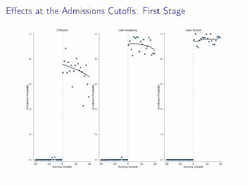
E�ects at the Admissions Cuto�s: First Stage
0.2
.4.6
.81
Enr
ollm
ent P
roba
bilit
y
−20 −10 0 10 20Running Variable
O’Bryant
0.2
.4.6
.81
Enr
ollm
ent P
roba
bilit
y
−20 −10 0 10 20Running Variable
Latin Academy
0.2
.4.6
.81
Enr
ollm
ent P
roba
bilit
y
−20 −10 0 10 20Running Variable
Latin School
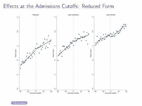
E�ects at the Admissions Cuto�s: Reduced Form
−.5
0.5
11.
52
Mea
n S
core
−20 −10 0 10 20Running Variable
O’Bryant
−.5
0.5
11.
52
Mea
n S
core
−20 −10 0 10 20Running Variable
Latin Academy
−.5
0.5
11.
52
Mea
n S
core
−20 −10 0 10 20Running Variable
Latin School
Estimates

Introduction
Latent Factor Modeling in a Sharp RD Design
Boston Exam Schools
Identi�cation and Estimation
Extrapolation Results
Counterfactual Simulations
Placebo Experiments
Conclusions
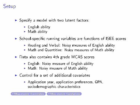
Setup
I Specify a model with two latent factors:
I English abilityI Math ability
I School-speci�c running variables are functions of ISEE scores
I Reading and Verbal: Noisy measures of English abilityI Math and Quantitive: Noisy measures of Math ability
I Data also contains 4th grade MCAS scores
I English: Noisy measure of English abilityI Math: Noisy measure of Math ability
I Control for a set of additional covariates
I Application year, application preferences, GPA,sociodemographic characteristics
Measurement Scatterplots Measurement Correlations

Estimation
I Measurement model: Maximum Simulated Likelihood[θE
θM
]| X ∼ N
([µ′θEX
µ′θM
X
],
[σ2
θEσθE θM
σθE θMσ2
θM
])
MEk | θ ,X ∼ N
(µ′
MEkX + λME
kθE ,exp
(γME
k+ δME
kθE
)2)
MMk | θ ,X ∼ N
(µ′
MMkX + λMM
kθM ,exp
(γMM
k+ δMM
kθM
)2)
I Latent outcome model: Method of Simulated Moments
E [Ds (z) | θ ,X ] = α′
Ds(z)X + β
EDs(z)
θE + βMDs(z)
θM
E [Y (S (z)) | θ ,X ] = α′
Y (S(z))X + βEY (S(z))θE + β
MY (S(z))θM
I Inference: 5-step bootstrap

Introduction
Latent Factor Modeling in a Sharp RD Design
Boston Exam Schools
Identi�cation and Estimation
Extrapolation Results
Counterfactual Simulations
Placebo Experiments
Conclusions

Preliminaries
Figure: Distribution of English and Math ability
Table: Factor loadings on ISEE and MCAS scores
Table: Dependence of outcomes on English and Math ability
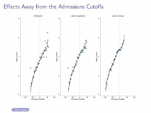
E�ects Away from the Admissions Cuto�s
−1
01
23
Mea
n S
core
−80 −40 0 40 80Running Variable
O’Bryant
−1
01
23
Mea
n S
core
−80 −40 0 40 80Running Variable
Latin Academy
−1
01
23
Mea
n S
core
−80 −40 0 40 80Running Variable
Latin School
Estimates
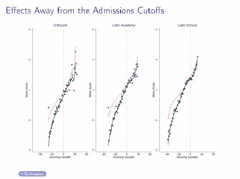
E�ects Away from the Admissions Cuto�s
−1
01
23
Mea
n S
core
−80 −40 0 40 80Running Variable
O’Bryant
−1
01
23
Mea
n S
core
−80 −40 0 40 80Running Variable
Latin Academy
−1
01
23
Mea
n S
core
−80 −40 0 40 80Running Variable
Latin School
Estimates
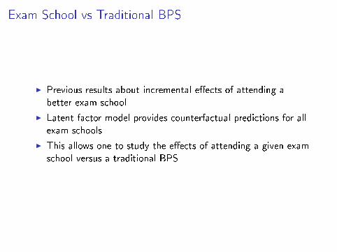
Exam School vs Traditional BPS
I Previous results about incremental e�ects of attending abetter exam school
I Latent factor model provides counterfactual predictions for allexam schools
I This allows one to study the e�ects of attending a given examschool versus a traditional BPS

Exam School vs Traditional BPS: All Applicantsextrapolation_all
Latin LatinO'Bryant Academy School
(1) (2) (3)First 0.754*** 0.948*** 0.968***Stage (0.020) (0.013) (0.016)
Reduced 0.021 0.049 0.024Form (0.037) (0.058) (0.064)
LATE 0.027 0.052 0.025(0.049) (0.062) (0.066)
N
Updated: 2014-01-13
* significant at 10%, ** significant at 5%, ***significant at 1%
3,704

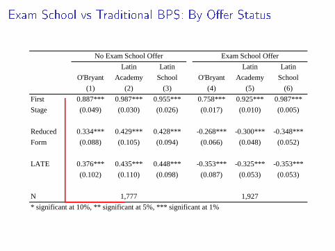
Exam School vs Traditional BPS: By O�er Status
extrapolation_atu_att
Latin Latin Latin LatinO'Bryant Academy School O'Bryant Academy School
(1) (2) (3) (4) (5) (6)First 0.887*** 0.987*** 0.955*** 0.758*** 0.925*** 0.987***Stage (0.049) (0.030) (0.026) (0.017) (0.010) (0.005)
Reduced 0.334*** 0.429*** 0.428*** -0.268*** -0.300*** -0.348***Form (0.088) (0.105) (0.094) (0.066) (0.048) (0.052)
LATE 0.376*** 0.435*** 0.448*** -0.353*** -0.325*** -0.353***(0.102) (0.110) (0.098) (0.087) (0.053) (0.053)
N
Updated: 2014-01-13
* significant at 10%, ** significant at 5%, *** significant at 1%
No Exam School Offer Exam School Offer
1,777 1,927
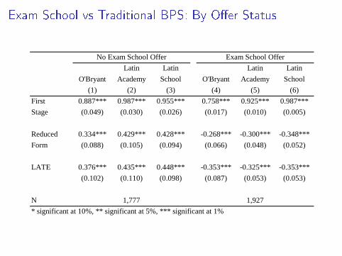
Miikka
Rectangle

Introduction
Latent Factor Modeling in a Sharp RD Design
Boston Exam Schools
Identi�cation and Estimation
Extrapolation Results
Counterfactual Simulations
Placebo Experiments
Conclusions
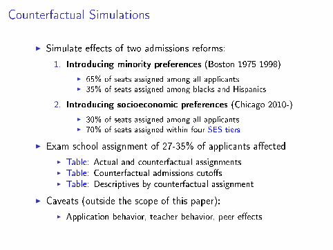
Counterfactual Simulations
I Simulate e�ects of two admissions reforms:
1. Introducing minority preferences (Boston 1975-1998)
I 65% of seats assigned among all applicantsI 35% of seats assigned among blacks and Hispanics
2. Introducing socioeconomic preferences (Chicago 2010-)
I 30% of seats assigned among all applicantsI 70% of seats assigned within four SES tiers
I Exam school assignment of 27-35% of applicants a�ected
I Table: Actual and counterfactual assignmentsI Table: Counterfactual admissions cuto�sI Table: Descriptives by counterfactual assignment
I Caveats (outside the scope of this paper):
I Application behavior, teacher behavior, peer e�ects

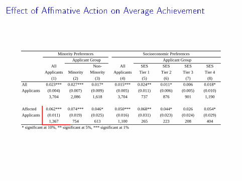
E�ect of A�mative Action on Average Achievement
cfsim12_effects
All Non- All SES SES SES SESApplicants Minority Minority Applicants Tier 1 Tier 2 Tier 3 Tier 4
(1) (2) (3) (4) (5) (6) (7) (8)All 0.023*** 0.027*** 0.017* 0.015*** 0.024** 0.011* 0.006 0.018*Applicants (0.004) (0.007) (0.009) (0.005) (0.011) (0.006) (0.005) (0.010)
3,704 2,086 1,618 3,704 737 876 901 1,190
Affected 0.062*** 0.074*** 0.046* 0.050*** 0.068** 0.044* 0.026 0.054*Applicants (0.011) (0.019) (0.025) (0.016) (0.031) (0.023) (0.024) (0.029)
1,367 754 613 1,100 265 223 208 404
Updated: 2014-01-13
* significant at 10%, ** significant at 5%, *** significant at 1%
Applicant GroupMinority Preferences
Applicant GroupSocioeconomic Preferences
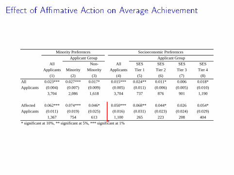
Miikka
Rectangle

Introduction
Latent Factor Modeling in a Sharp RD Design
Boston Exam Schools
Identi�cation and Estimation
Extrapolation Results
Counterfactual Simulations
Placebo Experiments
Conclusions

Placebo Experiments
Strategy:
1. Split data on applicants with assignment Z = 0,1,2,3 in halfbased on the median of the running variable
2. Re-estimate latent outcome models to the left and right of theplacebo cuto�s
3. Repeat reduced form extrapolations to the left and right of theplacebo cuto�s
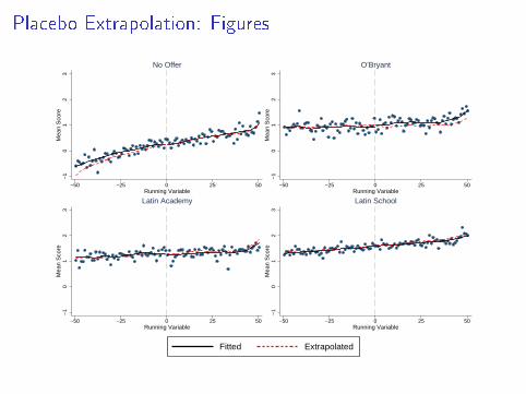
Placebo Extrapolation: Figures
−1
01
23
Mea
n S
core
−50 −25 0 25 50Running Variable
No Offer
−1
01
23
Mea
n S
core
−50 −25 0 25 50Running Variable
O’Bryant−
10
12
3M
ean
Sco
re
−50 −25 0 25 50Running Variable
Latin Academy
−1
01
23
Mea
n S
core
−50 −25 0 25 50Running Variable
Latin School
Fitted Extrapolated
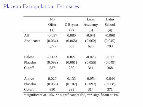
Placebo Extrapolation: Estimatesplacebo
No Latin LatinOffer O'Bryant Academy School(1) (2) (3) (4)
All -0.057 0.080 -0.041 -0.008Applicants (0.064) (0.068) (0.062) (0.045)
1,777 563 625 793
Below -0.133 0.027 -0.028 0.027Placebo (0.099) (0.061) (0.055) (0.049)Cutoff 887 280 311 368
Above 0.020 0.133 -0.054 -0.044Placebo (0.056) (0.102) (0.097) (0.068)Cutoff 890 283 314 371
Updated: 2014-01-13
* significant at 10%, ** significant at 5%, *** significant at 1%

Introduction
Latent Factor Modeling in a Sharp RD Design
Boston Exam Schools
Identi�cation and Estimation
Extrapolation Results
Counterfactual Simulations
Placebo Experiments
Conclusions
Conclusions
I Develop a latent factor-based approach to the extrapolation oftreatment e�ects away from the cuto� in RD
I Achievement gains from exam school attendance concentratedamong lower-scoring applicants
I A�rmative action predicted to increase average achievementamong a�ected applicants
I Latent factor-based extrapolation likely to be a promisingapproach also in various other RD designs
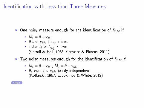
Identi�cation with Less than Three Measures
I One noisy measure enough for the identi�cation of fθ ,M if
I M1 = θ + νM1
I θ and νM1independent
I either fθ or fνM1known
(Carroll & Hall, 1988; Carrasco & Florens, 2011)
I Two noisy measures enough for the identi�cation of fθ ,M if
I M1 = θ + νM1, M2 = θ + νM2
I θ , νM1, and νM2
jointly independent(Kotlarski, 1967; Evdokimov & White, 2012)
Back
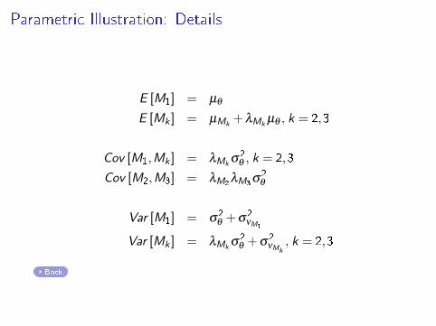
Parametric Illustration: Details
E [M1] = µθ
E [Mk ] = µMk+ λMk
µθ , k = 2,3
Cov [M1,Mk ] = λMkσ2θ , k = 2,3
Cov [M2,M3] = λM2λM3
σ2θ
Var [M1] = σ2θ + σ
2νM1
Var [Mk ] = λMkσ2θ + σ
2νMk
, k = 2,3
Back
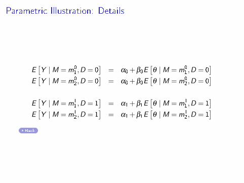
Parametric Illustration: Details
E[Y |M = m0
1,D = 0]
= α0 + β0E[θ |M = m0
1,D = 0]
E[Y |M = m0
2,D = 0]
= α0 + β0E[θ |M = m0
2,D = 0]
E[Y |M = m1
1,D = 1]
= α1 + β1E[θ |M = m1
1,D = 1]
E[Y |M = m1
2,D = 1]
= α1 + β1E[θ |M = m1
2,D = 1]
Back
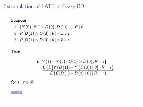
Extrapolation of LATE in Fuzzy RD
Suppose
1. (Y (0) ,Y (1) ,D (0) ,D (1))⊥⊥ R | θ2. P [D (1)≥ D (0) | θ ] = 1 a.s.
3. P [D (1) > D (0) | θ ] > 0 a.s.
Then
E [Y (1)−Y (0) | D (1) > D (0) ,R = r ]
=E {E [Y (D (1))−Y (D (0)) | θ ] | R = r}
E {E [D (1)−D (0) | θ ] | R = r}
for all r ∈R
Back

Settings with Multiple Latent Factors
I Suppose the data contains 2×K +1 noisy measures of latentfactors θ1, . . . ,θK :
Mk1 = gMk
1
(θk ,νMk
1
), k = 1, . . . ,K
Mk2 = gMk
2
(θk ,νMk
2
), k = 1, . . . ,K
M3 = gW (θ1, . . . ,θK ,νM3)
Mk1 and Mk
2 , k = 1, . . . ,K , continuous, M3 potentially discrete
I R is a deterministic function of a subset of M = (M1,M2,M3)
I Extending all of the identi�cation results to this settingrequires only slight modi�cations
Back

Deferred Acceptance Algorithm
I Round 1: Applicants are considered for a seat in their mostpreferred exam school. Each exam schools rejects thelowest-ranking applicants in excess of its capacity. The rest ofthe applicants are provisionally admitted.
I Round k > 1: Applicants rejected in Round k−1 areconsidered for a seat in their next most preferred exam school.Each exam schools considers these applicants together withthe provisionally admitted applicants from Round k−1 andrejects the lowest-ranking students in excess of its capacity.The rest of the students are provisionally admitted.
I The algorithm terminates once either each applicants areassigned an o�er from one of the exam schools or allunmatched applicant are rejected by every exam school in theirpreference ordering.
Back
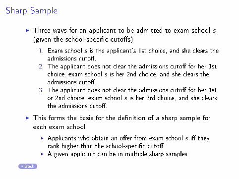
Sharp Sample
I Three ways for an applicant to be admitted to exam school s(given the school-speci�c cuto�s)
1. Exam school s is the applicant's 1st choice, and she clears theadmissions cuto�.
2. The applicant does not clear the admissions cuto� for her 1stchoice, exam school s is her 2nd choice, and she clears theadmissions cuto�.
3. The applicant does not clear the admissions cuto� for her 1stor 2nd choice, exam school s is her 3rd choice, and she clearsthe admissions cuto�.
I This forms the basis for the de�nition of a sharp sample foreach exam school
I Applicants who obtain an o�er from exam school s i� theyrank higher than the school-speci�c cuto�
I A given applicant can be in multiple sharp samples
Back

Descriptive Statistics
descriptives
All All No Latin Latin
BPS Applicants Offer O'Bryant Academy School
(1) (2) (3) (4) (5) (6)
Female 0.489 0.545 0.516 0.579 0.581 0.577
Black 0.516 0.399 0.523 0.396 0.259 0.123
Hispanic 0.265 0.189 0.223 0.196 0.180 0.081
FRPL 0.755 0.749 0.822 0.788 0.716 0.499
LEP 0.116 0.073 0.109 0.064 0.033 0.004
Bilingual 0.315 0.387 0.353 0.420 0.451 0.412
SPED 0.227 0.043 0.073 0.009 0.006 0.009
English 4 0.000 0.749 0.251 0.870 1.212 1.858
Math 4 0.000 0.776 0.206 0.870 1.275 2.114
N 21,094 5,179 2,791 755 790 843
Updated: 2013-11-08
Exam School Assignment
Back
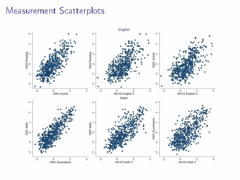
Measurement Scatterplots
−2
−1
01
23
ISE
E R
eadi
ng
−2 0 2 4ISEE Verbal
.
−2
−1
01
23
ISE
E R
eadi
ng−2 0 2 4
MCAS English 4
English
−2
−1
01
23
ISE
E V
erba
l
−2 0 2 4MCAS English 4
.−
2−
10
12
3IS
EE
Mat
h
−2 0 2 4ISEE Quantitative
.
−2
−1
01
23
ISE
E M
ath
−2 0 2 4MCAS Math 4
Math
−2
−1
01
23
ISE
E Q
uant
itativ
e
−2 0 2 4MCAS Math 4
.

Measurement Scatterplots (cont'd)
−2
02
4M
CA
S E
nglis
h 4
−2 0 2 4MCAS Math 4
Back

Measurement Correlations
measurement_correlations
Reading Verbal Math Quantitative English 4 Math 4
(1) (2) (3) (4) (5) (6)
Reading 1 0.735 0.631 0.621 0.670 0.581
Verbal 0.735 1 0.619 0.617 0.655 0.587
Math 0.631 0.619 1 0.845 0.598 0.740
Quantitative 0.621 0.617 0.845 1 0.570 0.718
English 4 0.670 0.655 0.598 0.570 1 0.713
Math 4 0.581 0.587 0.740 0.718 0.713 1.000
N
Updated: 2013-11-08
Panel B: MCAS
Panel A: ISEE
ISEE MCAS
5,179
Back
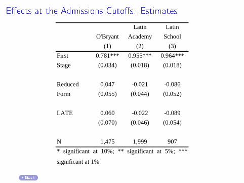
E�ects at the Admissions Cuto�s: Estimatesrd_estimates_all
Latin Latin
O'Bryant Academy School
(1) (2) (3)
First 0.781*** 0.955*** 0.964***
Stage (0.034) (0.018) (0.018)
Reduced 0.047 -0.021 -0.086
Form (0.055) (0.044) (0.052)
LATE 0.060 -0.022 -0.089
(0.070) (0.046) (0.054)
N 1,475 1,999 907
Updated: 2013-11-08
* significant at 10%; ** significant at 5%; ***
significant at 1%
Back
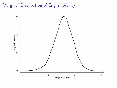
Marginal Distribution of English Ability
0.2
.4.6
Mar
gina
l Den
sity
−2 0 2 4English Ability
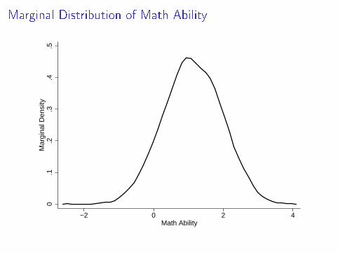
Marginal Distribution of Math Ability
0.1
.2.3
.4.5
Mar
gina
l Den
sity
−2 0 2 4Math Ability

Scatterplot of English and Math Ability
−1
01
23
4E
nglis
h A
bilit
y
−2 0 2 4Math Ability
Back
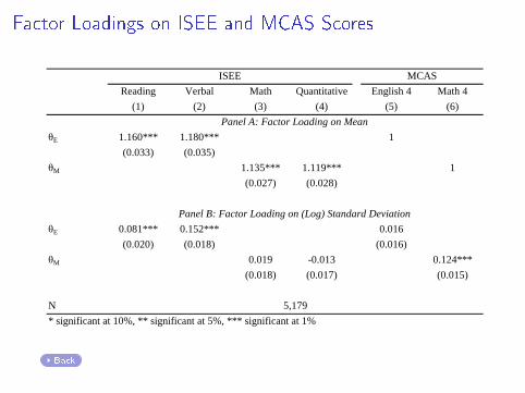
Factor Loadings on ISEE and MCAS Scoresfactor_loadings
Reading Verbal Math Quantitative English 4 Math 4(1) (2) (3) (4) (5) (6)
θE 1.160*** 1.180*** 1(0.033) (0.035)
θM 1.135*** 1.119*** 1(0.027) (0.028)
θE 0.081*** 0.152*** 0.016(0.020) (0.018) (0.016)
θM 0.019 -0.013 0.124***(0.018) (0.017) (0.015)
N
Updated: 2014-01-13
* significant at 10%, ** significant at 5%, *** significant at 1%5,179
Panel B: Factor Loading on (Log) Standard Deviation
ISEE MCAS
Panel A: Factor Loading on Mean
Back
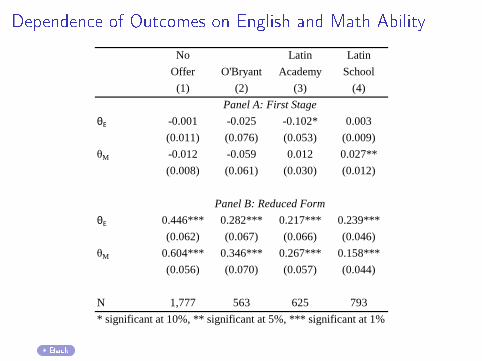
Dependence of Outcomes on English and Math Abilitylatent_fs_rf
No Latin LatinOffer O'Bryant Academy School(1) (2) (3) (4)
θE -0.001 -0.025 -0.102* 0.003(0.011) (0.076) (0.053) (0.009)
θM -0.012 -0.059 0.012 0.027**(0.008) (0.061) (0.030) (0.012)
θE 0.446*** 0.282*** 0.217*** 0.239***(0.062) (0.067) (0.066) (0.046)
θM 0.604*** 0.346*** 0.267*** 0.158***(0.056) (0.070) (0.057) (0.044)
N 1,777 563 625 793
Updated: 2014-01-13
Panel A: First Stage
* significant at 10%, ** significant at 5%, *** significant at 1%
Panel B: Reduced Form
Back
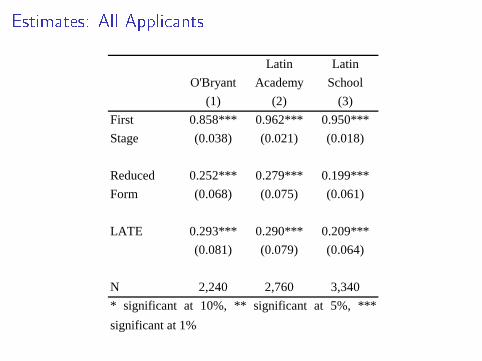
Estimates: All Applicantsrd_extrapolation_all
Latin LatinO'Bryant Academy School
(1) (2) (3)First 0.858*** 0.962*** 0.950***Stage (0.038) (0.021) (0.018)
Reduced 0.252*** 0.279*** 0.199***Form (0.068) (0.075) (0.061)
LATE 0.293*** 0.290*** 0.209***(0.081) (0.079) (0.064)
N 2,240 2,760 3,340
Updated: 2014-01-13
* significant at 10%, ** significant at 5%, ***significant at 1%
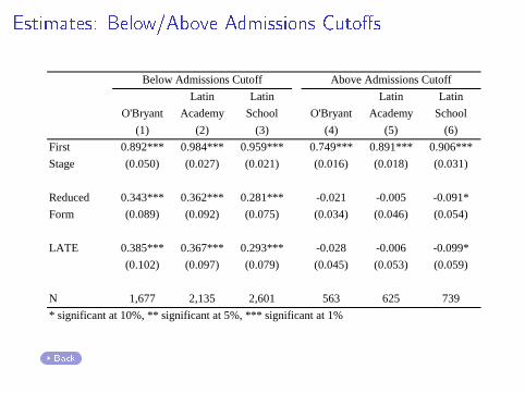
Estimates: Below/Above Admissions Cuto�srd_extrapolation_cutoff
Latin Latin Latin LatinO'Bryant Academy School O'Bryant Academy School
(1) (2) (3) (4) (5) (6)First 0.892*** 0.984*** 0.959*** 0.749*** 0.891*** 0.906***Stage (0.050) (0.027) (0.021) (0.016) (0.018) (0.031)
Reduced 0.343*** 0.362*** 0.281*** -0.021 -0.005 -0.091*Form (0.089) (0.092) (0.075) (0.034) (0.046) (0.054)
LATE 0.385*** 0.367*** 0.293*** -0.028 -0.006 -0.099*(0.102) (0.097) (0.079) (0.045) (0.053) (0.059)
N 1,677 2,135 2,601 563 625 739
Updated: 2014-01-13
* significant at 10%, ** significant at 5%, *** significant at 1%
Below Admissions Cutoff Above Admissions Cutoff
Back
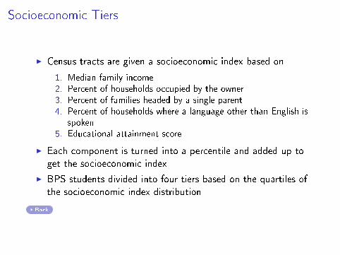
Socioeconomic Tiers
I Census tracts are given a socioeconomic index based on
1. Median family income2. Percent of households occupied by the owner3. Percent of families headed by a single parent4. Percent of households where a language other than English is
spoken5. Educational attainment score
I Each component is turned into a percentile and added up toget the socioeconomic index
I BPS students divided into four tiers based on the quartiles ofthe socioeconomic index distribution
Back
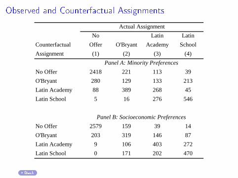
Observed and Counterfactual Assignmentscfsim12_assignments
No Latin Latin
Counterfactual Offer O'Bryant Academy School
Assignment (1) (2) (3) (4)
No Offer 2418 221 113 39
O'Bryant 280 129 133 213
Latin Academy 88 389 268 45
Latin School 5 16 276 546
No Offer 2579 159 39 14
O'Bryant 203 319 146 87
Latin Academy 9 106 403 272
Latin School 0 171 202 470
Updated: 2013-11-08
Actual Assignment
Panel A: Minority Preferences
Panel B: Socioeconomic Preferences
Back
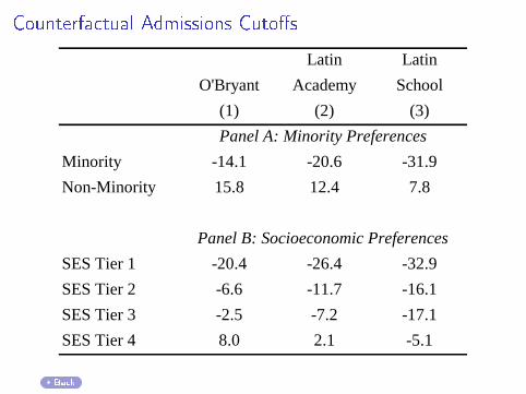
Counterfactual Admissions Cuto�scfsim12_cutoffs
Latin Latin
O'Bryant Academy School
(1) (2) (3)
Minority -14.1 -20.6 -31.9
Non-Minority 15.8 12.4 7.8
SES Tier 1 -20.4 -26.4 -32.9
SES Tier 2 -6.6 -11.7 -16.1
SES Tier 3 -2.5 -7.2 -17.1
SES Tier 4 8.0 2.1 -5.1
Updated: 2013-11-08
Panel A: Minority Preferences
Panel B: Socioeconomic Preferences
Notes: This table reports the differences between the actual
admissions cutoffs and the counterfactual admissions
cutoffs under minority and socioeconomic preferences in
the exam school admissions.
Back
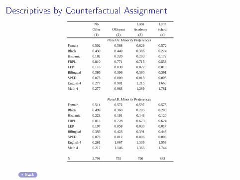
Descriptives by Counterfactual Assignmentcfsim12_descriptives
No Latin Latin
Offer O'Bryant Academy School
(1) (2) (3) (4)
Female 0.502 0.588 0.629 0.572
Black 0.430 0.440 0.386 0.274
Hispanic 0.182 0.220 0.203 0.172
FRPL 0.810 0.771 0.715 0.556
LEP 0.116 0.030 0.022 0.018
Bilingual 0.386 0.396 0.380 0.391
SPED 0.073 0.009 0.013 0.005
English 4 0.277 0.981 1.215 1.668
Math 4 0.277 0.963 1.289 1.781
Female 0.514 0.572 0.597 0.575
Black 0.499 0.360 0.295 0.203
Hispanic 0.223 0.191 0.143 0.120
FRPL 0.813 0.728 0.673 0.624
LEP 0.107 0.058 0.030 0.017
Bilingual 0.359 0.423 0.391 0.445
SPED 0.073 0.012 0.006 0.006
English 4 0.261 1.067 1.309 1.556
Math 4 0.217 1.146 1.365 1.744
N 2,791 755 790 843
Updated: 2013-11-08
Panel A: Minority Preferences
Panel B: Minority Preferences
Back