Public perceptions of disabled people: evidence from the British ...
Jobs and Climate Policy:Evidence from British Columbia’s Revenue-Neutral
Carbon Tax∗
Akio Yamazaki†
Version: December 2015
Working Paper
Abstract
This paper examines the employment impact of British Columbia’s revenue-neutral carbontax implemented in 2008. While all industries appear to benefit from the redistributed taxrevenues, the most carbon-intensive and trade-sensitive industries see employment fall withthe tax, while clean service industries see employment rise. By aggregating across industriesI find the BC carbon tax generated a small but statistically significant 2 percent increase inemployment over the 2007-2013 period. This paper provides initial evidence showing how arevenue-neutral carbon tax may not adversely affect employment.
Key Words: Environmental regulation; carbon tax; employment; unilateral climate policy
JEL Codes: E24, H23, J2, Q5∗Previous versions of this paper was circulated with the title ”On the Employment Effects of Climate Policy:
The Evidence from Carbon Tax in British Columbia.” I am very grateful to my advisors, Jared C. Carbone and M.Scott Taylor, for their great supervision and invaluable advice. The paper also benefited from extensive discussionswith Pamela Campa, Arvind Magesan, Kenneth J. McKenzie, Nicolas Rivers, Brandon Schaufele, Stefan Staubli, andTrevor Tombe. I also thank Jevan Cherniwchan, Eugene Choo, Matthew Webb, Matthew Winden, and seminar par-ticipants at CREE Annual Conference 2014, EEPRN 2nd Annual Research Symposium 2014, MEA Annual Meeting2015, University of Calgary for their helpful comments. All remaining errors are my own.
†University of Calgary, Department of Economics, 2500 University Dr. N.W., Calgary, AB, T2N 1N4, Canada.Email: [email protected] Phone: (403)220-5857 Fax: (403)282-5262
1. Introduction
Despite half a century of experience in Europe and North America with environmental regu-
lations, their likely impacts are still heavily debated.1 For example, many believe that such reg-
ulations could lead to substantial layoffs due to major adjustments or the shutdown of firms, and
that these costs outweigh any potential environmental benefits. However, others believe that such
regulations could strengthen the economy by creating more green jobs.2 While both job gains and
losses are, in fact, reported, understanding the relationship between environmental regulations and
jobs is difficult because every regulation is unique in its design and impact.3 To better inform poli-
cymakers and the public about the effect of environmental regulations on jobs, this paper examines
the employment effect of the revenue-neutral carbon tax in British Columbia (BC).
On July 1st, 2008, BC implemented a carbon tax on the purchase of all fossil fuels. This
policy intervention has several unique and useful characteristics that make it an ideal natural ex-
periment with which to study its employment effect. First, the tax was implemented relatively
quickly, specifically only five months after its announcement. This ruled out the possibility that
polluters would adjust their behavior in anticipation of the regulation. Second, the tax coverage
was comprehensive as the tax was levied on all sources of carbon emissions from all industries.
This comprehensive industrial coverage allows me to identify both job gains and losses across in-
dustries in response to the regulation. Third, the tax rate was set relatively high, which provided
a strong signal to polluters to change their behavior when the policy was introduced. Last, it was
designed to be revenue-neutral, i.e., all the tax revenue raised went to the reduction of personal and
corporate income taxes and provided lump-sum transfers to low-income households. Recycling
tax revenues could raise the income of BC residents and is an important part of the policy because
1Examples of the environmental regulations in the earlier years are the Clean Air Act of 1956 in the United King-dom (Brimblecombe, 2006) and the Clean Air Act in the United States (US EPA, 2013).
2A definition of a green job is loosely defined as a job that contributes substantially to preserving or restoringenvironmental quality (United Nations Environment Programme, 2008).
3For example, the Cross-State Air Pollution rule, implemented in 2011, had eliminated 500 jobs in Texas (Boyle,2011). Hundreds of miners have been laid off due to EPA’s new clean power policy (Cama, 2015). On the otherhand, green jobs have been created in green goods and services in the United States. Between 2010 and 2011, theconstruction sector created 100,000 green jobs (Grenoble, 2013).
1
it could stimulate the labor market in BC. Many researchers have argued that lowering the personal
income tax reduces distortion in the existing tax system and raises labor supply, which is referred
to as the double dividend hypothesis.4 However, one must also realize that the employment impact
could come from the demand side, especially when the corporate income tax was also lowered.
Therefore, this policy feature allows me to discuss the possibility of a demand side story of the
double dividend hypothesis.
My empirical strategy is motivated by a simple labor market model. The model illustrates that
there are three channels through which a revenue-neutral carbon tax affects employment. First, the
tax reduces labor demand due to a decrease in output, which I call an output effect. In a long-run
competitive equilibrium, the tax increases marginal costs, shifting the perfectly horizontal supply
curve upward and raising price. As a result, output declines. Such decline would be large if demand
is highly elastic and production is emission-intensive. Second, redistributing tax revenues could
positively affect both labor demand and supply, which I call a redistribution effect. Recycling
tax revenues to lower personal income tax and provide lump-sum transfers could stimulate labor
demand through increases in product demand. Product demand could rise due to the spending of
redistributed tax revenue by BC residents, thus raising outputs. In addition, lowering corporate
income tax (CIT) could also stimulate labor demand because it reduces the burden of CIT from
labor in the form of higher wages. At the same time, recycling the revenues to lower the labor
tax could reduce the distortion in the labor market, thus increasing the labor supply. Lastly, labor
demand could increase if energy is easily substitutable with labor, which I call a factor substitution
effect. Depending on the size of these offsetting factors, the employment effects could differ across
industries, and an overall employment effect is ambiguous.
I used industry-level data to decompose the employment effect into the output and redistri-
bution effect. As the output effect depends on both demand elasticity and emission intensity, I
explicitly allowed the output effect to be identified separately based on these factors. Lacking
demand elasticity data, I proxy for the elasticity with trade intensity. This is because some argue
4This is often called the employment dividend when the non-environmental dividend is an increase in employmentalone (Carraro, Galeotti and Gallo, 1996).
2
that industries targeting world markets face relatively elastic demand while industries targeting
mainly domestic markets face relatively inelastic demand. The redistribution effect is identified
using constructed tax revenue data for BC, i.e., interacting the tax rate with BC’s aggregate an-
nual greenhouse gas (GHG) emissions. Using this strategy, the employment effect is identified by
a difference-in-difference estimator allowing for differential treatment intensity across industries.
This method compares changes in employment for industries in BC with changes in employment
for industries in the rest of Canada before and after the unilateral implementation of the carbon
tax. To clearly identify the employment effect, I exploit the panel structure of data by including
various fixed effects to control for possible unobserved confounding factors, such as commodity
price shocks, provincial geographic characteristics, and national economic growth.
I find that the output effect negatively affects employment for all industries but differently based
on emission and trade intensity while the redistribution effect positively affects employment for all
industries. The most carbon-intensive and trade-sensitive industries see employment fall with the
tax while clean service industries see employment rise. For example, at $10/t carbon dioxide
equivalent (CO2e), the basic chemical manufacturing sector, one of the most emission-intensive
and trade-exposed industries, experiences the largest decline in employment at 30 percent. On the
other hand, the health care service sector, one of the clean and domestic industries, experiences
the largest increase in employment at 16 percent.5 By aggregating the employment effects across
industries, I find the BC carbon tax generated a small but statistically significant 2 percent increase
in employment over the 2007-2013 period.
Although a large number of studies in the literature have examined the relationship between
jobs and environmental regulations, especially during the 80’s and 90’s using simulation meth-
ods, most studies have mainly focused on pollution control regulations, such as the Clean Air Act
(CAA) of the United States.6 Only a handful of studies, such as Berman and Bui (2001) and
5This does not imply that when the tax rate reaches $30/t CO2, the size of employment effects would simply bethree times as much. It does, however, mean that if the tax rate is set initially at $30/t CO2, the employment effectswould be three times as much.
6To name a few, see Hollenbeck (1979), Environmental Protection Agency (1981), Bezdek, Wendling and Jones(1989), Wendling and Bezdek (1989), and Hazilla and Kopp (1990).
3
Greenstone (2002), econometrically investigated this relationship. What is missing from this liter-
ature are more studies examining the employment effect of a climate policy. Thus far, only Martin,
de Preux and Wagner (2014) have investigated the effect of the UK’s carbon tax, the Climate
Change Levy (CCL), on manufacturing activities. Their results found no statistically significant
impact of such tax on employment. This paper differs from Martin, de Preux and Wagner in several
ways. First, although the CCL is considered a carbon tax, the CCL and BC carbon tax are designed
differently, especially in sectoral coverage and exemptions.7 Second, this paper investigated the
net effect of the carbon tax by considering many different sectors while Martin, de Preux and Wag-
ner only focused on the manufacturing sector. For these reasons, this paper provides new evidence
for the relationship between jobs and environmental regulations by investigating the employment
effects of the BC carbon tax.
This paper also contributes to the literature on double dividend by providing empirical evidence
to support the employment dividend hypothesis. While all empirical studies in this literature have
used simulation methods, this is the first study examining this hypothesis econometrically.8 Boven-
berg and Goulder (2002) argue that an environmental tax reform, i.e., recycling the revenue from
an environmental tax to reduce the rates of other distortionary taxes, can increase employment.
This hypothesis holds on the basis of two conditions: industries facing the tax are not exception-
ally labor-intensive and revenue is recycled to lower the labor tax. Although this paper does not
provide a direct empirical test of the employment dividend hypothesis, the BC carbon tax appears
to generate an employment dividend because these conditions are satisfied for the case of the BC
carbon tax. In addition, I investigate the effect of the BC carbon tax on provincial wages, and find
that the tax has a statistically significant negative effect. This finding suggests that the increase
in aggregate employment partly comes from the rightward shift of labor supply, which provides
further evidence of the employment dividend.
Methodologically, this paper is closely related to Berman and Bui (2001) and Greenstone
7The CCL is a per unit tax only on industrial energy use. A 90 percent discount on the tax rate is applied if afirm voluntary commits to an emission reduction target by participating in the Climate Change Agreement. Therefore,although the CCL is a national-level carbon tax, the coverage was quite limited.
8See Majocchi (1996) and Bosquet (2000) for a survey of empirical evidence.
4
(2002). Both papers examined the employment effect of air pollution regulations by using a
difference-in-difference approach. Berman and Bui analyzed the employment impact of the lo-
cal air pollution regulation on the manufacturing sector in Los Angeles (LA).9 They found a small
increase (2,600 to 5,400) in employment over the 1979-1991 period. Greenstone investigated the
employment effect of the Clean Air Act Amendments (CAAA) on the manufacturing sector in U.S.
counties during the 1972-1987 period. His results showed that the regulation decreased employ-
ment by roughly 590,000.
Although these papers came to opposing conclusions, their results are consistent with my find-
ings. Berman and Bui (2001) argued that one of the potential reasons for their small positive
employment effects is that manufacturing plants in LA are not trade-intensive because their market
is mainly local. Based on my simple model, this suggests that the negative output effect on labor
demand is likely to be small for the LA manufacturing plants. On the other hand, I argue that the
negative output effect for Greenstone (2002) might be large as the manufacturing plants across the
entire U.S. are more trade-intensive. The key element that led to the different results between these
two papers appears to be the difference in the degree of trade intensity in the manufacturing plants.
Therefore, although these studies both focus on the manufacturing sector, it makes sense that their
employment effects differ. The negative employment effects for BC’s manufacturing industries in
this paper also stem from their high trade intensity. Understanding the characteristics of sectors
facing the regulation could help predict the outcome of future policies. .
The rest of the paper proceeds as follows. Section 2 describes the details of the construction and
the implementation of the BC carbon tax. Section 3 uses a simple model to identify the channels
through which a revenue-neutral carbon tax affects employment. Section 4 contains my empirical
analysis where I explain data and methodology, and provide results and robustness checks. Then
I discuss how the carbon tax affects provincial wages and provide support for the employment
dividend in Section 5. Finally, Section 6 concludes.
9To be precise, their region of interest is South Coast Air Basin, which includes Los Angeles County, OrangeCounty, Riverside County, and the non-desert portion of San Bernardino County.
5
2. Overview of the BC Carbon Tax
On February 2007, Premier Gordon Campbell announced BC’s new climate policy agenda
in his throne speech (Harrison, 2012). The Liberal government, led by Premier Campbell, had
previously undergone deep cuts to the environmental budget and supported offshore oil and gas
exploration. The announcement came as a surprise to many, including members of his own party
(Harrison, 2012). In October 2007, the Ministry of Finance publicly acknowledged that a carbon
tax is under consideration, and officially announced the implementation in their budget plan in
February 2008. The tax was implemented relatively quickly, specifically only five months after
its announcement. Although the announcement of the tax took the public by surprise, polls in-
dicated that 72 percent felt that the introduction of a carbon tax is a positive step (Duff, 2008).
Others, including businesses and industry associations, worried about the adverse effects on their
operational costs and requested tax relief or exemptions (Ministry of Finance, 2013). Overall, the
implementation of the carbon tax has been supported by BC residents as the Liberal party has won
the majority of seats in the 2009 and 2013 post-carbon tax elections.
The BC carbon tax is levied on the carbon content of all fossil fuels, including gasoline, diesel,
natural gas, coal, propane, and home heating fuel (Ministry of Finance, 2008), from all industries.
Often some forms of exemptions are granted to protect the domestic economy, such as energy-
intensive and trade-exposed industries. The exemption usually makes the tax relatively narrow-
based. However, the BC carbon tax is considered to be broad-based because exemptions were
initially applied to none of the industries.10
According to the Budget and Fiscal Plan (Ministry of Finance, 2014), the carbon tax raised
$1.1 billion revenue for 2012-2013 and is estimated to raise about $1.2 billion revenue for 2013-
2014. As the BC carbon tax is designed to be revenue-neutral, all the tax revenue raised goes to the
10This has been changed as of March, 2012. To protect agricultural industries, a carbon tax relief was granted tocommercial greenhouse growers. A temporary relief of $7.6 million was provided in 2012, and then the relief programwas made into a permanent program in 2013. As of January 1, 2014, the farmers are exempted from the carbontax on the purchase of colored gasoline and colored diesel fuel used for farm purposes. For further information, seehttp:www.gov.bc.ca/agri/.
6
reduction of personal and corporate income taxes and provides lump-sum transfers to low-income
households (Ministry of Finance, 2008). The corporate income tax and the two lowest personal
income tax were reduced by 5 percent. These made BC’s corporate and personal income taxes
the lowest in Canada (Elgie and McClay, 2013).11 In addition, the BC government provides a
lump-sum credit to protect low-income households. Although the government had designed this
policy to be a revenue-neutral carbon tax, tax credits have been exceeding tax revenues since its
implementation. For example, the excess was $260 million in 2012-2013. This discrepancy stems
from failing to accurately estimate the expected revenue from the carbon tax. How the revenues
would be recycled is determined before the actual amount of revenue collected is known, thus
keeping the policy exactly revenue-neutral is a difficult task. The estimated revenues have been
lower than anticipated since the implementation due to the much higher decline in consumption of
fossil fuels. Although the policy has been revenue-negative, given that the excesses account only
for less than 1 percent of BC’s total tax revenue, I treat it as revenue-neutral in this analysis to be
consistent with the intention of the BC government.
In the tax’s initial year of 2008, the rate was set at $10/t CO2e from burning fossil fuels and
scheduled to increase by $5/t CO2e annually until 2012. This means that the carbon tax would
increase 2.41 cents per liter for gasoline, rising gradually to 7.24 cents a liter by 2012 (Ministry
of Finance, 2008). The gradual increase of the tax rate allows consumers to adjust their fuel usage
slowly and minimize the financial burden from the tax.
Only several years have passed since the implementation of the BC carbon tax, but there has
already been a significant reduction in the use of fossil fuels and GHG emissions. A recent report
(Elgie and McClay, 2013) showed that the per capita use of fossil fuels in BC has declined by 17
percent during the first four years following its implementation, which is 19 percent more than in
the rest of Canada. Similarly, the per capita GHG emissions have declined by 10 percent in BC
from 2008 to 2011. Thus far, the BC carbon tax appears to be fulfilling its purpose.
11In fact, BC has tied with Alberta and New Brunswick for the lowest corporate tax rate, and has had the lowestpersonal income tax rate in Canada, but for only those earnings up to $119,000.
7
3. A Model of Jobs and Carbon Tax
In this section, I use a simple model to identify the channels through which a revenue-neutral
carbon tax affects employment. The different channels are illustrated using simple diagrams, but a
formal mathematical representation of the model is presented in Online Appendix.
To illustrate that the employment effect could differ across industries, two industries are con-
sidered under a long-run competitive equilibrium, industry A and industry B. Industry A is an
energy-intensive industry facing relatively elastic demand while industry B is a clean industry
facing relatively inelastic demand.
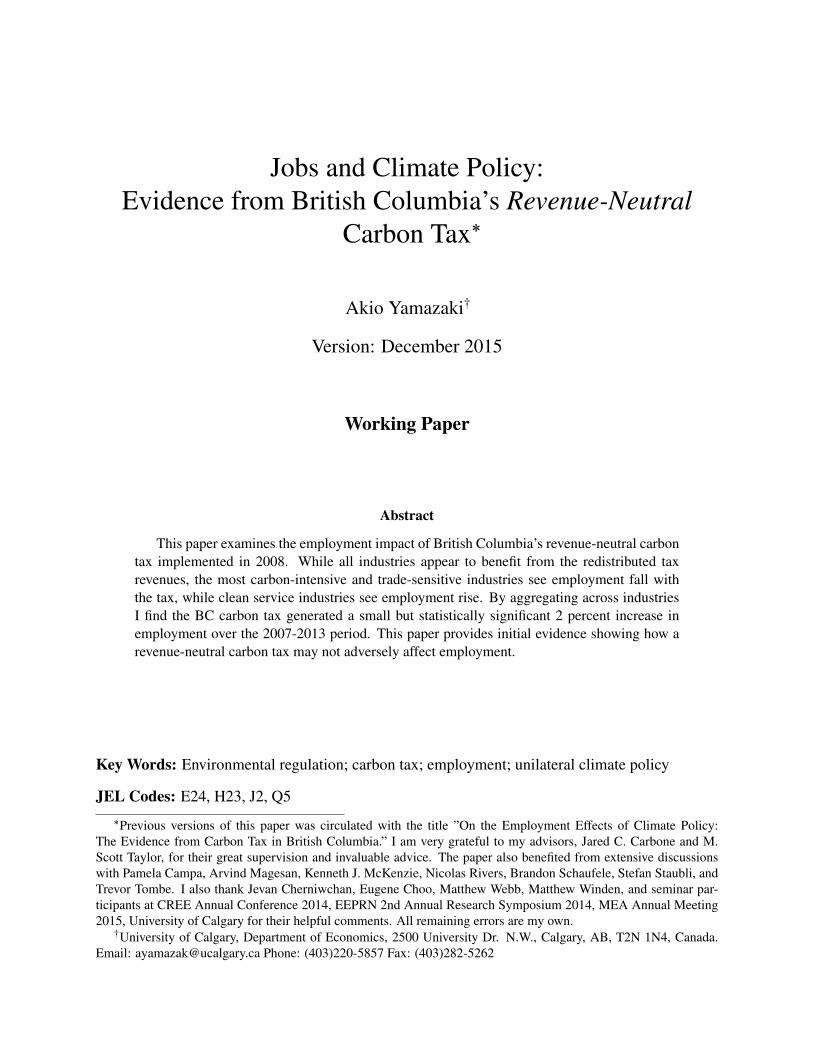
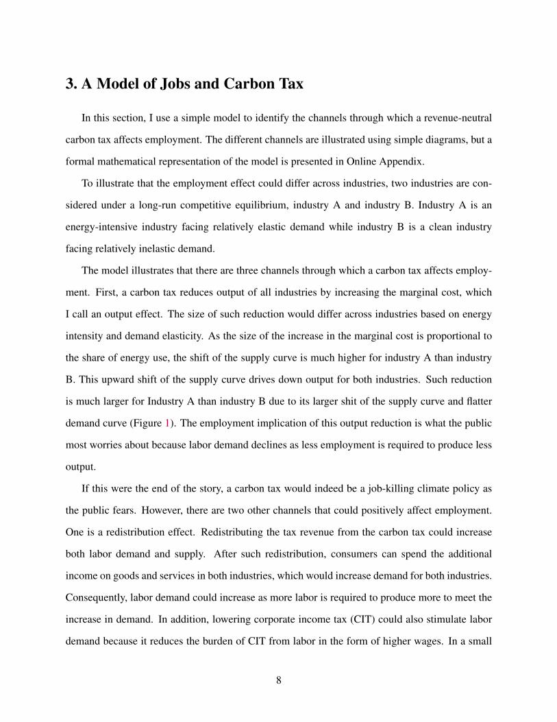
The model illustrates that there are three channels through which a carbon tax affects employ-
ment. First, a carbon tax reduces output of all industries by increasing the marginal cost, which
I call an output effect. The size of such reduction would differ across industries based on energy
intensity and demand elasticity. As the size of the increase in the marginal cost is proportional to
the share of energy use, the shift of the supply curve is much higher for industry A than industry
B. This upward shift of the supply curve drives down output for both industries. Such reduction
is much larger for Industry A than industry B due to its larger shit of the supply curve and flatter
demand curve (Figure 1). The employment implication of this output reduction is what the public
most worries about because labor demand declines as less employment is required to produce less
output.
If this were the end of the story, a carbon tax would indeed be a job-killing climate policy as
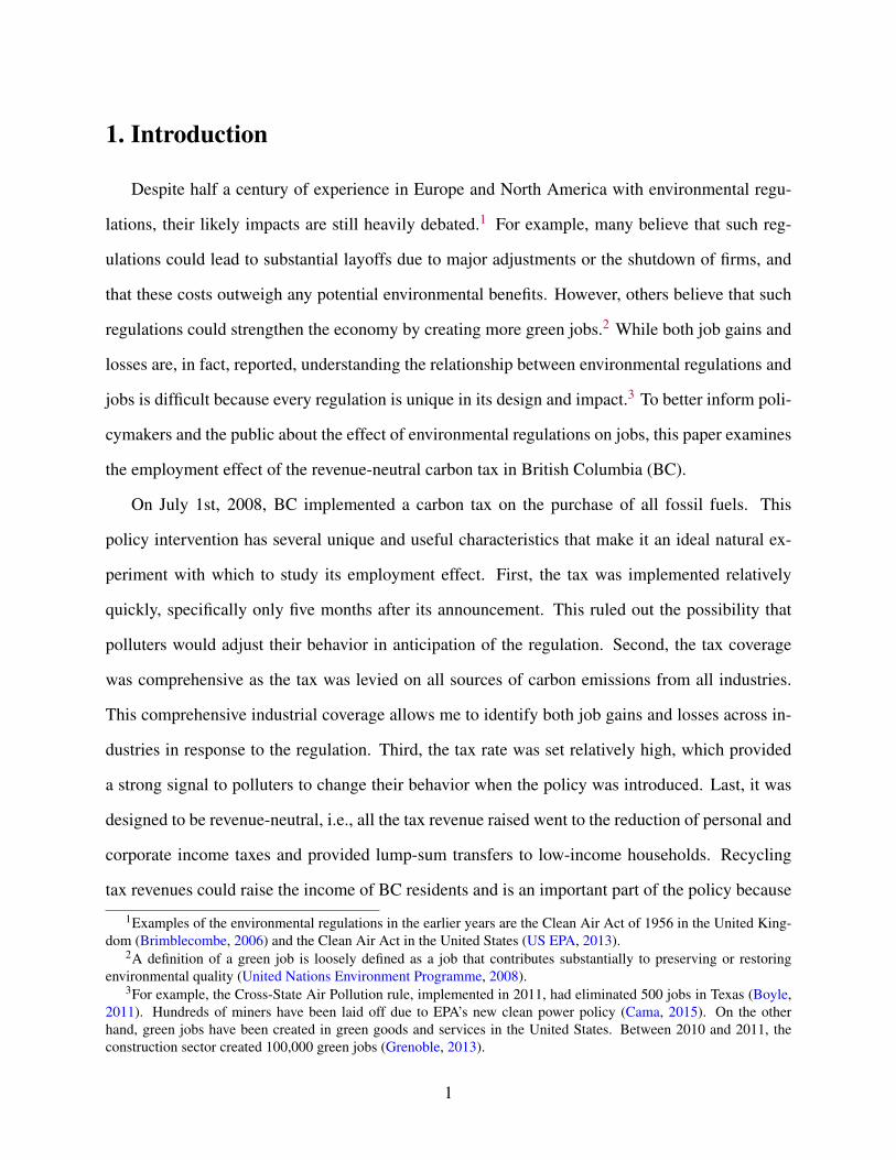
the public fears. However, there are two other channels that could positively affect employment.
One is a redistribution effect. Redistributing the tax revenue from the carbon tax could increase
both labor demand and supply. After such redistribution, consumers can spend the additional
income on goods and services in both industries, which would increase demand for both industries.
Consequently, labor demand could increase as more labor is required to produce more to meet the
increase in demand. In addition, lowering corporate income tax (CIT) could also stimulate labor
demand because it reduces the burden of CIT from labor in the form of higher wages. In a small
8
𝑞1 𝑞0 𝑞0 𝑞1
D
MC1
𝑝
𝑞
𝑝
𝑞
MC2
MC1
D
MC2
Industry A Industry B
Figure 1: Negative Output Effects
Note: Industry A is an energy-intensive industry facing relatively elastic demand while industry B is a clean industryfacing relatively inelastic demand.
open economy, the incidence of CIT falls on labor when capital is mobile across regions (Kotlikoff
and Summer, 1987). This is because capital would flee from a region with CIT, which lowers labor
productivity and thus wages. Therefore, lowering CIT would shift labor demand curve outward.
At the same time, the reduction of personal income tax by revenue-recycling could increase labor
supply among BC residents because it reduces the distortion in the labor market, which is referred
to as the employment divided hypothesis. The redistribution effect could thus increase employment
through both an increase in labor demand and supply. The other is a factor substitution effect. If
an industry can easily switch from energy to labor to lessen the tax burden, labor demand may
increase. The larger the elasticity of the factor substitution is, the larger the positive effect on labor
demand.
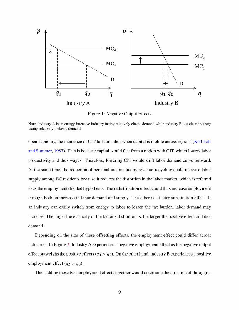
Depending on the size of these offsetting effects, the employment effect could differ across
industries. In Figure 2, Industry A experiences a negative employment effect as the negative output
effect outweighs the positive effects (q0 > q2). On the other hand, industry B experiences a positive
employment effect (q2 > q0).
Then adding these two employment effects together would determine the direction of the aggre-
9
𝑞1 𝑞0 𝑞2 𝑞2 𝑞0 𝑞1
D2 D
1
D2
MC1
𝑝
𝑞
𝑝
𝑞
MC2
MC1
D1
MC2
Industry A Industry B
Figure 2: Positive Redistribution Effects
Note: Industry A is an energy-intensive industry facing relatively elastic demand while industry B is a clean industryfacing relatively inelastic demand.
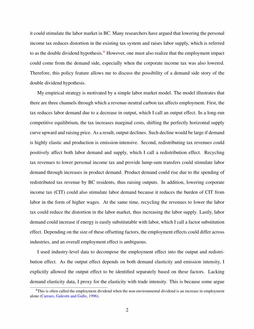
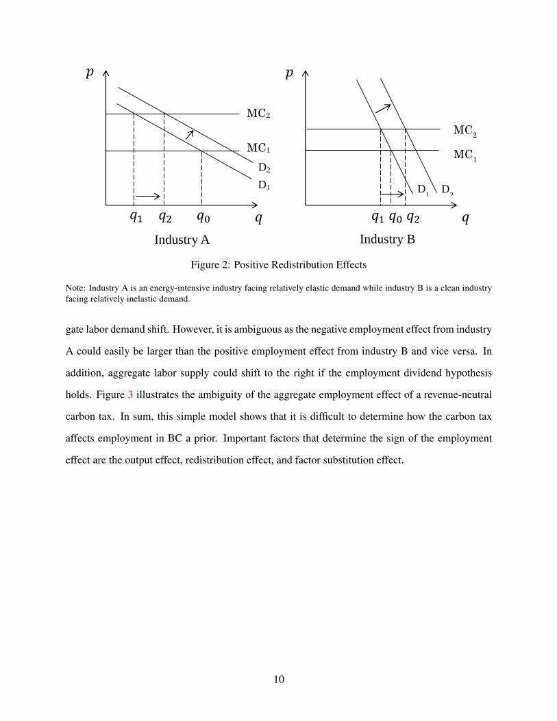
gate labor demand shift. However, it is ambiguous as the negative employment effect from industry
A could easily be larger than the positive employment effect from industry B and vice versa. In
addition, aggregate labor supply could shift to the right if the employment dividend hypothesis
holds. Figure 3 illustrates the ambiguity of the aggregate employment effect of a revenue-neutral
carbon tax. In sum, this simple model shows that it is difficult to determine how the carbon tax
affects employment in BC a prior. Important factors that determine the sign of the employment
effect are the output effect, redistribution effect, and factor substitution effect.
10
L*
LS
∑LD
L
W
W*
Figure 3: Aggregate Employment Effect
4. Empirical Analysis
I. Data Sources
To examine the employment effect of the BC carbon tax, annual data on employment, GHG
emission intensity, and trade intensity are obtained from Statistics Canada.12 The simple model
illustrated that the output effect depends on energy intensity and demand elasticity. Lacking such
data, I proxy for energy intensity with emission intensity based on the assumption that GHG emis-
sion intensity is proportional to energy intensity. I also proxy demand elasticity with trade intensity
as the degree of trade-exposure is a good representation of demand elasticity.
Constructing the dataset requires manual merging as the industry classification used for em-
ployment and GHG emission intensity data is slightly different from the commodity classification
used for trade intensity data. Table A.1 in the Data Appendix documents the concordance between
these two classifications. After merging data, 68 industries, 12 regions (9 provinces and 3 terri-
tories), and 13 years (2001-2013) are covered in the data.13 Descriptive statistics are reported in
12See the Data Appendix for further details on the data construction.13Quebec introduced a carbon policy in 2007 as well; however, given that Quebec’s carbon tax rate is set at much
11
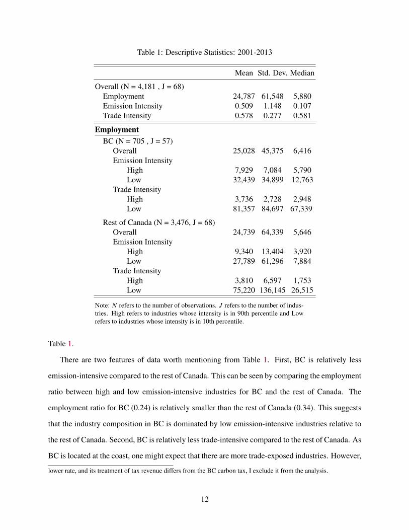
Table 1: Descriptive Statistics: 2001-2013
Mean Std. Dev. Median
Overall (N = 4,181 , J = 68)Employment 24,787 61,548 5,880Emission Intensity 0.509 1.148 0.107Trade Intensity 0.578 0.277 0.581
EmploymentBC (N = 705 , J = 57)
Overall 25,028 45,375 6,416Emission Intensity
High 7,929 7,084 5,790Low 32,439 34,899 12,763
Trade IntensityHigh 3,736 2,728 2,948Low 81,357 84,697 67,339
Rest of Canada (N = 3,476, J = 68)Overall 24,739 64,339 5,646Emission Intensity
High 9,340 13,404 3,920Low 27,789 61,296 7,884
Trade IntensityHigh 3,810 6,597 1,753Low 75,220 136,145 26,515
Note: N refers to the number of observations. J refers to the number of indus-tries. High refers to industries whose intensity is in 90th percentile and Lowrefers to industries whose intensity is in 10th percentile.
Table 1.
There are two features of data worth mentioning from Table 1. First, BC is relatively less
emission-intensive compared to the rest of Canada. This can be seen by comparing the employment
ratio between high and low emission-intensive industries for BC and the rest of Canada. The
employment ratio for BC (0.24) is relatively smaller than the rest of Canada (0.34). This suggests
that the industry composition in BC is dominated by low emission-intensive industries relative to
the rest of Canada. Second, BC is relatively less trade-intensive compared to the rest of Canada. As
BC is located at the coast, one might expect that there are more trade-exposed industries. However,
lower rate, and its treatment of tax revenue differs from the BC carbon tax, I exclude it from the analysis.
12
there are more workers in less trade-exposed industries in BC than in the rest of Canada. These
industry composition in terms of emission intensity and trade intensity are important elements for
determining the size of the employment effects of the carbon tax.
There are several potential concerns about data. First, Statistics Canada provides industrial
GHG emission data only at national level and only from 1990 to 2008. On the contrary, employ-
ment data is available across industries for all provinces from 2001 to 2013. To make use of this
limited data, an assumption is imposed — national GHG emission intensity level for each industry
serves as a proxy for each industry in all provinces. While the emission intensity level might be
different across provinces for each industry, the relative emission intensity level across industries
within provinces is likely to be the same. For instance, a relatively dirty industry in Alberta, such
as the oil and gas extraction, would also be a relatively dirty industry in other provinces. Therefore,
GHG emission intensity data at national level is sufficient.
To examine the employment effect of the carbon tax, only emission intensity variation across
industries in the pre-carbon tax period is required. With data for more post-carbon tax years, one
could examine an effect of the carbon tax on the level of GHG emissions. However, that is not the
purpose of this study. GHG emission intensity is likely to decline in BC after the implementation
of the carbon tax; yet, the relative emission intensity across industries is unlikely to change (i.e., a
dirty industry will not suddenly become a clean industry solely due to the implementation of the
carbon tax). Therefore, not having data for the post-carbon tax period is not problematic.
Second, trade intensity data are available by commodities, provinces, and years, but only covers
the period from 2007 to 2011.14 As trade intensity after 2008 is also likely to be affected by the
carbon tax (i.e., trade intensity could be an outcome variable), only data from the pre-carbon tax
period are used in the analysis. As for the GHG emission intensity, exploiting trade intensity
variation across industries and provinces at the pre-carbon tax period is sufficient for this analysis.
To justify the use of these data only from 2007, I ranked the industries in order of intensity over
14The trade intensity data for 1997-2008 is available from Table 386-0002; however, this table does not provideinformation on a commodity classification ID, which makes the manual merging difficult. As Table 386-0002 and386-0003 are not fully comparable, trade intensity data for prior to 2007 was not utilized in the analysis.
13
020
4060
80
Ran
king
in 1
997
0 20 40 60 80
Ranking in 2007
Emission Intensity
010
2030
4050
6070
Ran
king
in 2
007
0 10 20 30 40 50 60 70
Ranking in 2011
Trade Intensity
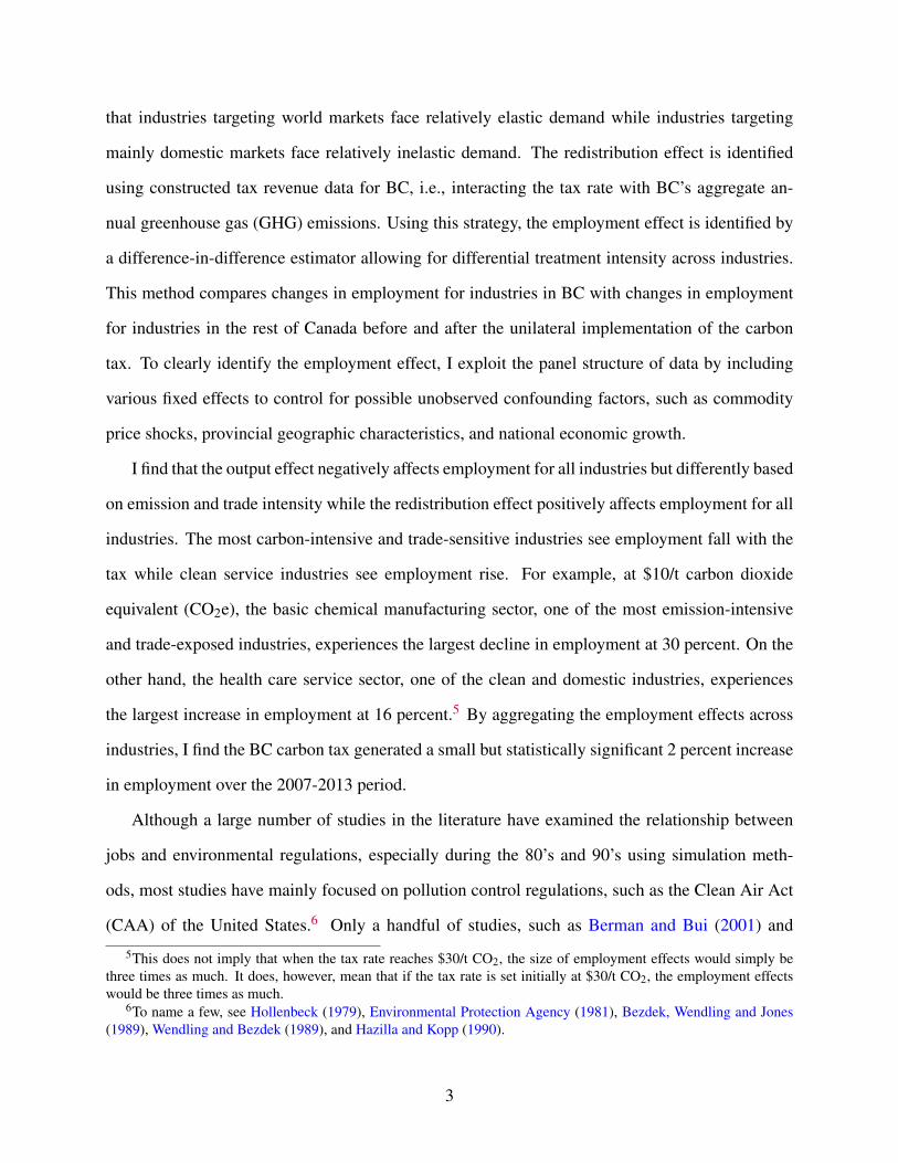
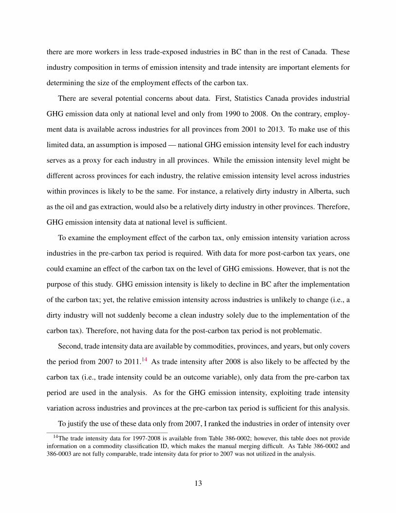
Figure 4: Emissin Intensity & Trade Intensity Ranking
Note: Industries are ranked based on their emission intensity and trade intensity level. Rank No.1 means the lowestintensity in the sample.Source: Author’s calculation.
time and plotted them in Figure 4. If the relative intensity among industries are constant over time,
the data would line up on the 45-degree line. Except for a few outliers, emission intensity ranking
in 1997 appears to be preserved in 2007. Similarly, trade intensity ranking in 2007 are maintained
in 2011. These suggest that the relative intensity in emission and trade are fairly constant over
time.
II. Methodology
This section discusses the econometric design to estimate the employment effect of BC’s
revenue-neutral carbon tax. The simple model illustrated that the employment effects depend on
three effects: the output effect, redistribution effect, and factor substitution effect. With available
data, I attempt to separately identify the output effect and redistribution effect as follows:
ln L i pt = β1(E Ii × BC p × τt)+ β2(T radei p × BC p × τt) (4.1)
+ β3(G H G p × BC p × τt)+ λi + ηp + δi t + µp f (t)+ γt + εi pt
14
where ln L i pt is the natural log of employment for industry i in province p at time t .15 Let E Ii
be a GHG emission intensity level for industry i in 2007, T radei p be trade intensity for industry i
at province p in 2007, G H G p be total GHG emissions in BC at 2007, BC p be a dummy variable
for BC, and τt be a carbon tax variable (i.e., 0 if t = pre-carbon tax period, 10 if t = 2008, 15 if
t = 2009, ..., 30 if t = 2012, and 30 if t = 2013).16 λi are industry fixed effects that capture time-
invariant industry heterogeneity, such as industry factor intensity. ηp are province fixed effects
that control for time-invariant province heterogeneity, such as geographic characteristics and factor
endowments. δi t are industry-specific time fixed effects that controls for industry specific shocks at
given year. Controlling for industry-specific shocks are particularly important as this will control
for incidences such as the financial crisis, exogenous changes in prices of natural resources and
commodities, and any shocks that are specific to industries but common across provinces. µp f (t)
are second-order polynomial province-specific time trends that control for differential province
specific trends, such as a provincial growth. γt are time fixed effects that capture aggregate shocks
that are common across industries and provinces, such as economic growth at the national level.
Finally, εi pt is an error term that captures idiosyncratic changes in employment.
The first three interaction terms capture the employment effect of the BC carbon tax through
different channels. The first interaction term measures the output effect through energy intensity.
The second interaction term measures the output effect through demand elasticity. The third in-
teraction term captures the redistribution effect. By interacting the carbon tax variable with BC’s
total GHG emission from 2007, a tax revenue variable is constructed to estimate the redistribution
effect of the tax.17
In addition, using emission and trade intensity in the estimation is attractive because it allows
me to discuss the employment effect of the carbon tax on emission-intensive and trade-exposed
15The natural log of employment is employed to remove the skewness in the distribution of employment. After thetransformation, employment is approximately distributed normal.
16The use of BC p × τt to measure the stringency of the policy is inspired by Rivers and Schaufele (2014). Theyinvestigated an effect of the BC carbon tax on agricultural trade.
17In Online Appendix, I also estimate the redistribution effect (β̂3) of the carbon tax more directly using data on theactual amount of tax revenue rebated, reported in BC’s budget plan. As the amount of rebate is potentially endogenousto labor supply decisions, using this variable in the estimation could be problematic. Therefore, the rebate variable isconstructed as G H G p × BC p × τt .
15
(EITE) industries. When environmental regulations are imposed, policymakers often worry that
the financial burden from complying with the regulations falls harshly on EITE industries.18 As
the product price for EITE industries is determined at the world market, they are unable to mitigate
the additional burden from the regulations by passing on the increased costs to consumers. As a
result, the employment effect of the carbon tax for EITE industries might be largely negative.
The coefficients of interest are β1, β2, and β3. In particular, the approximate percentage
change in employment for industry i at time t in response to the carbon tax is calculated by
αi t ≡ 100 × (β̂1 E Ii + β̂2T radei p + β̂3G H G p)1τt .19 The estimated coefficient β̂1 and β̂2 are
identified from across industry × province comparisons over time and β̂3 is identified from across
provincial comparisons over time. To properly identify the employment effect, the underlying
identification assumption requires that there be no factors other than the carbon tax creating differ-
ences in changes in employment between industries in BC and industries in other provinces. This
assumption will be violated if the government of BC concurrently implements other policy induced
by the carbon tax that affects all industries in BC differently while no other provinces implement a
similar policy.
Another important identification assumption is common trends. This assumption requires that
the changes in employment for industries in BC (treatment group) and other provinces (control
group) would follow the same time trend in the absence of the carbon tax. Although verifying this
assumption is difficult, one can compare the mean employment growth rate in the pre-treatment
period between BC and the rest of Canada (ROC). This allows me to check if there is a systematic
difference in employment trends between these groups. This can be done by performing a t-test
on the difference in mean employment growth rates during the pre-carbon tax period between BC
and ROC (Table 2). The test fails to reject the null hypothesis that the difference in group means is
different from zero, suggesting that there is no significant difference in pre-treatment employment
trends between the treatment and control group.
18See Morgenstern (2010) for an example of U.S. Clean Air Act.19As the estimation equation is in the semi-elasticity (log-linear) form, the exact percentage change in employment
is calculated by 100×(
e(β̂1 E Ii+β̂2T radei p+β̂3G H G p)1τt − 1)
.
16
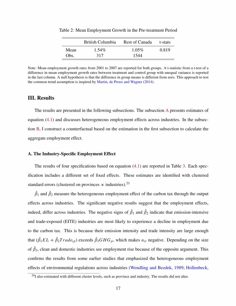
Table 2: Mean Employment Growth in the Pre-treatment Period
British Columbia Rest of Canada t-stats
Mean 1.54% 1.05% 0.819Obs. 317 1544
Note: Mean employment growth rates from 2001 to 2007 are reported for both groups. A t-statistic from a t-test of adifference in mean employment growth rates between treatment and control group with unequal variance is reportedin the last column. A null hypothesis is that the difference in group means is different from zero. This approach to testthe common trend assumption is inspired by Martin, de Preux and Wagner (2014).
III. Results
The results are presented in the following subsections. The subsection A presents estimates of
equation (4.1) and discusses heterogeneous employment effects across industries. In the subsec-
tion B, I construct a counterfactual based on the estimation in the first subsection to calculate the
aggregate employment effect.
A. The Industry-Specific Employment Effect
The results of four specifications based on equation (4.1) are reported in Table 3. Each spec-
ification includes a different set of fixed effects. These estimates are identified with clustered
standard errors (clustered on provinces × industries).20
β̂1 and β̂2 measure the heterogeneous employment effect of the carbon tax through the output
effects across industries. The significant negative results suggest that the employment effects,
indeed, differ across industries. The negative signs of β̂1 and β̂2 indicate that emission-intensive
and trade-exposed (EITE) industries are most likely to experience a decline in employment due
to the carbon tax. This is because their emission intensity and trade intensity are large enough
that (β̂1 E Ii + β̂2T radei p) exceeds β̂3G H G p, which makes αi t negative. Depending on the size
of β̂3, clean and domestic industries see employment rise because of the opposite argument. This
confirms the results from some earlier studies that emphasized the heterogeneous employment
effects of environmental regulations across industries (Wendling and Bezdek, 1989; Hollenbeck,
20I also estimated with different cluster levels, such as province and industry. The results did not alter.
17
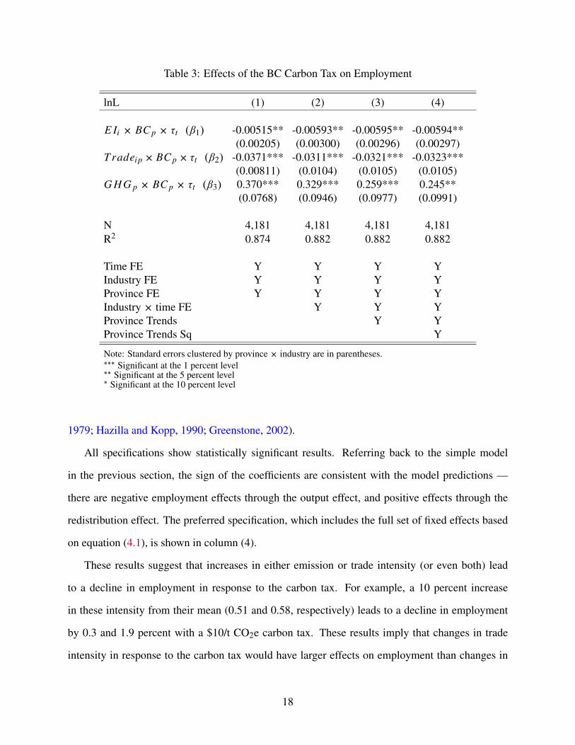
Table 3: Effects of the BC Carbon Tax on Employment
lnL (1) (2) (3) (4)
E Ii × BC p × τt (β1) -0.00515** -0.00593** -0.00595** -0.00594**(0.00205) (0.00300) (0.00296) (0.00297)
T radei p× BC p× τt (β2) -0.0371*** -0.0311*** -0.0321*** -0.0323***(0.00811) (0.0104) (0.0105) (0.0105)
G H G p × BC p × τt (β3) 0.370*** 0.329*** 0.259*** 0.245**(0.0768) (0.0946) (0.0977) (0.0991)
N 4,181 4,181 4,181 4,181R2 0.874 0.882 0.882 0.882
Time FE Y Y Y YIndustry FE Y Y Y YProvince FE Y Y Y YIndustry × time FE Y Y YProvince Trends Y YProvince Trends Sq Y
Note: Standard errors clustered by province × industry are in parentheses.∗∗∗ Significant at the 1 percent level∗∗ Significant at the 5 percent level∗ Significant at the 10 percent level
1979; Hazilla and Kopp, 1990; Greenstone, 2002).
All specifications show statistically significant results. Referring back to the simple model
in the previous section, the sign of the coefficients are consistent with the model predictions —
there are negative employment effects through the output effect, and positive effects through the
redistribution effect. The preferred specification, which includes the full set of fixed effects based
on equation (4.1), is shown in column (4).
These results suggest that increases in either emission or trade intensity (or even both) lead
to a decline in employment in response to the carbon tax. For example, a 10 percent increase
in these intensity from their mean (0.51 and 0.58, respectively) leads to a decline in employment
by 0.3 and 1.9 percent with a $10/t CO2e carbon tax. These results imply that changes in trade
intensity in response to the carbon tax would have larger effects on employment than changes in
18
b1EIi+b3GHGp
-20
-15
-10
-50
510
1520
Em
ploy
men
t effe
ct (
%)
0 1 2 3 4 5
Emission Intensity (t/$1,000 production)
b2Tradeip+b3GHGp
-20
-15
-10
-50
510
1520
Em
ploy
men
t effe
ct (
%)
0 .25 .5 .75 1
Trade Intensity
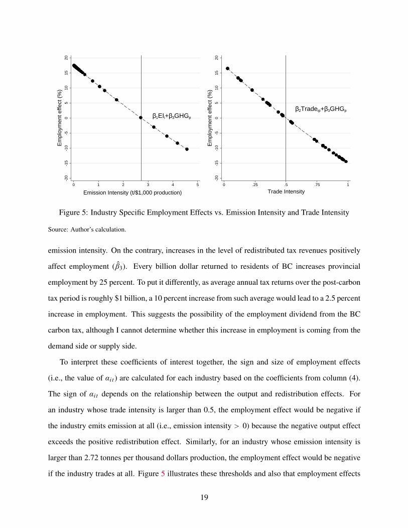
Figure 5: Industry Specific Employment Effects vs. Emission Intensity and Trade Intensity
Source: Author’s calculation.
emission intensity. On the contrary, increases in the level of redistributed tax revenues positively
affect employment (β̂3). Every billion dollar returned to residents of BC increases provincial
employment by 25 percent. To put it differently, as average annual tax returns over the post-carbon
tax period is roughly $1 billion, a 10 percent increase from such average would lead to a 2.5 percent
increase in employment. This suggests the possibility of the employment dividend from the BC
carbon tax, although I cannot determine whether this increase in employment is coming from the
demand side or supply side.
To interpret these coefficients of interest together, the sign and size of employment effects
(i.e., the value of αi t ) are calculated for each industry based on the coefficients from column (4).
The sign of αi t depends on the relationship between the output and redistribution effects. For
an industry whose trade intensity is larger than 0.5, the employment effect would be negative if
the industry emits emission at all (i.e., emission intensity > 0) because the negative output effect
exceeds the positive redistribution effect. Similarly, for an industry whose emission intensity is
larger than 2.72 tonnes per thousand dollars production, the employment effect would be negative
if the industry trades at all. Figure 5 illustrates these thresholds and also that employment effects
19
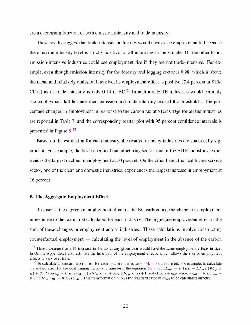
are a decreasing function of both emission intensity and trade intensity.
These results suggest that trade-intensive industries would always see employment fall because
the emission intensity level is strictly positive for all industries in the sample. On the other hand,
emission-intensive industries could see employment rise if they are not trade-intensive. For ex-
ample, even though emission intensity for the forestry and logging sector is 0.98, which is above
the mean and relatively emission intensive, its employment effect is positive (7.4 percent at $10/t
CO2e) as its trade intensity is only 0.14 in BC.21 In addition, EITE industries would certainly
see employment fall because their emission and trade intensity exceed the thresholds. The per-
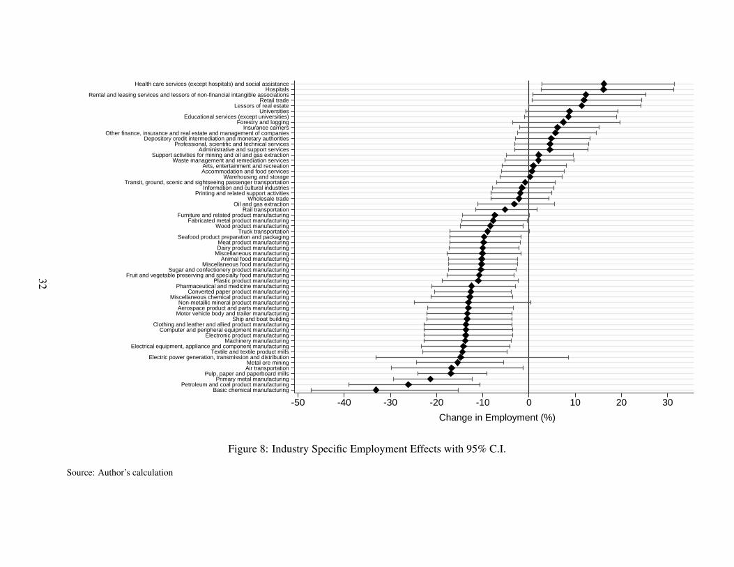
centage changes in employment in response to the carbon tax at $10/t CO2e for all the industries
are reported in Table 7, and the corresponding scatter plot with 95 percent confidence intervals is
presented in Figure 8.22
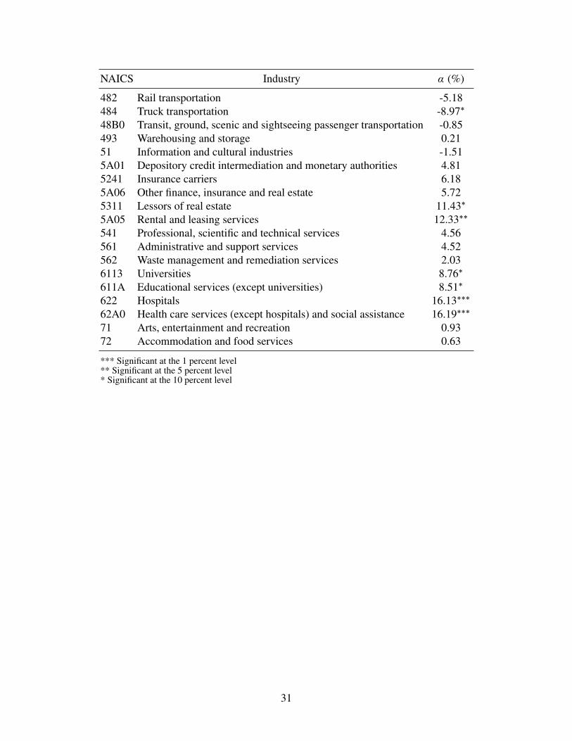
Based on the estimation for each industry, the results for many industries are statistically sig-
nificant. For example, the basic chemical manufacturing sector, one of the EITE industries, expe-
riences the largest decline in employment at 30 percent. On the other hand, the health care service
sector, one of the clean and domestic industries, experiences the largest increase in employment at
16 percent.
B. The Aggregate Employment Effect
To discuss the aggregate employment effect of the BC carbon tax, the change in employment
in response to the tax is first calculated for each industry. The aggregate employment effect is the
sum of these changes in employment across industries. These calculations involve constructing
counterfactual employment — calculating the level of employment in the absence of the carbon
21Here I assume that a $1 increase in the tax at any given year would have the same employment effects in size.In Online Appendix, I also estimate the time path of the employment effects, which allows the size of employmenteffects to vary over time.
22To calculate a standard error of αi t for each industry, the equation (4.1) is transformed. For example, to calculatea standard error for the coal mining industry, I transform the equation (4.1) as ln L i pt = β1(E Ii − E Icoal)(BC p ×
τt )+ β2(T radei p − T radecoal, BC)(BC p × τt )+ αcoal(BC p × τt )+ Fixed effects+ εi pt where αcoal = β1 E Icoal +
β3T radecoal,BC + β3G H G BC . This transformation allows the standard error of αcoal to be calculated directly.
20
68
1012
Log
of E
mpl
oym
ent
0 1 2 3 4 5
Emission Intensity
68
1012
Log
of E
mpl
oym
ent
0 .2 .4 .6 .8 1
Trade Intensity
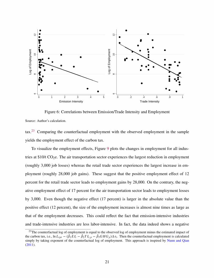
Figure 6: Correlations between Emission/Trade Intensity and Employment
Source: Author’s calculation.
tax.23 Comparing the counterfactual employment with the observed employment in the sample
yields the employment effect of the carbon tax.
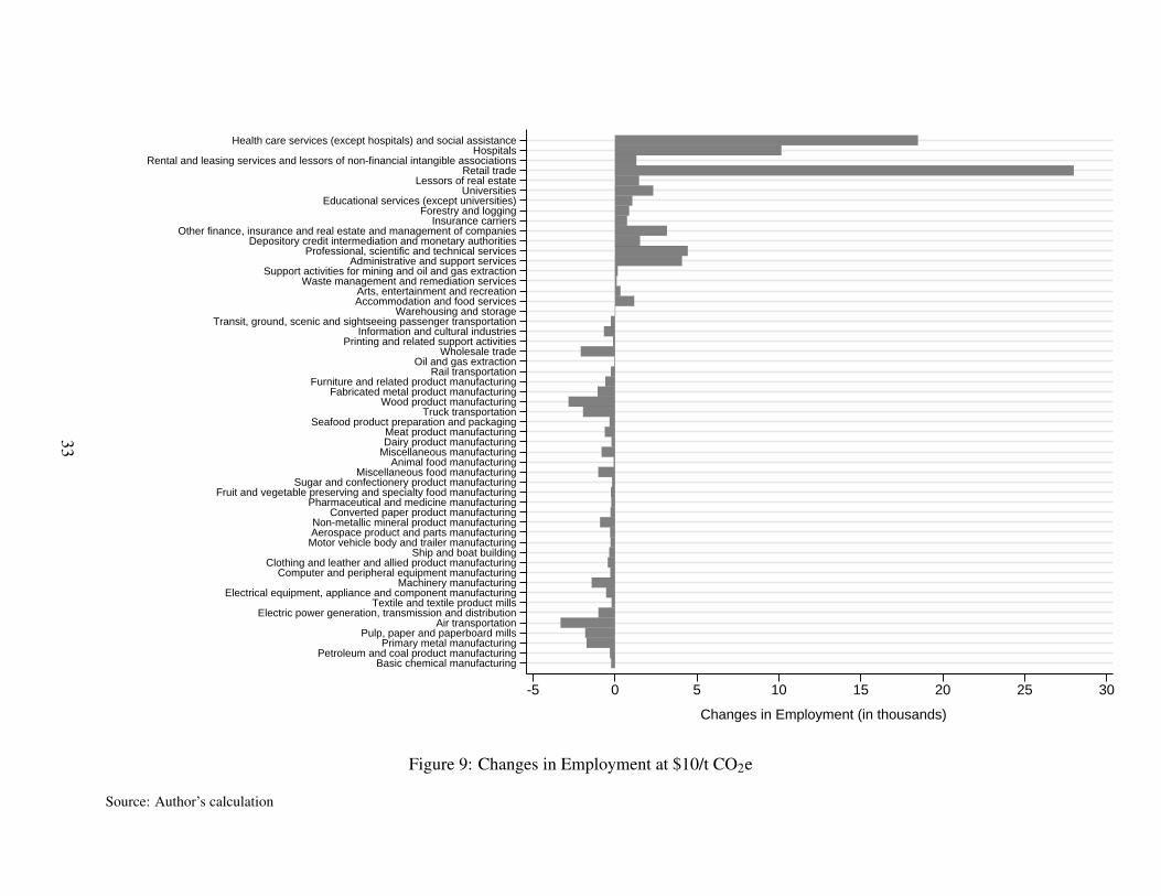
To visualize the employment effects, Figure 9 plots the changes in employment for all indus-
tries at $10/t CO2e. The air transportation sector experiences the largest reduction in employment
(roughly 3,000 job losses) whereas the retail trade sector experiences the largest increase in em-
ployment (roughly 28,000 job gains). These suggest that the positive employment effect of 12
percent for the retail trade sector leads to employment gains by 28,000. On the contrary, the neg-
ative employment effect of 17 percent for the air transportation sector leads to employment losses
by 3,000. Even though the negative effect (17 percent) is larger in the absolute value than the
positive effect (12 percent), the size of the employment increases is almost nine times as large as
that of the employment decreases. This could reflect the fact that emission-intensive industries
and trade-intensive industries are less labor-intensive. In fact, the data indeed shows a negative
23The counterfactual log of employment is equal to the observed log of employment minus the estimated impact ofthe carbon tax, i.e., ln L i pt − (β̂1 E Ii − β̂2T Ii,p − β̂3G H G p)1τt . Then the counterfactual employment is calculatedsimply by taking exponent of the counterfactual log of employment. This approach is inspired by Nunn and Qian(2011).
21
1.35
1.4
1.45
1.5
Tot
al E
mpl
oym
ent (
in m
illio
n)
2007 2008 2009 2010 2011 2012 2013
Carbon Tax (Observed)
No Carbon Tax
Upper 90%
Lower 90%
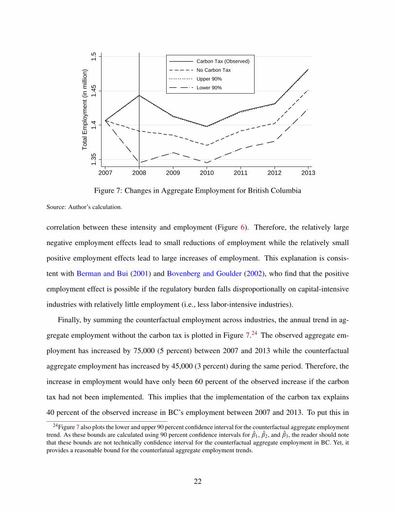
Figure 7: Changes in Aggregate Employment for British Columbia
Source: Author’s calculation.
correlation between these intensity and employment (Figure 6). Therefore, the relatively large
negative employment effects lead to small reductions of employment while the relatively small
positive employment effects lead to large increases of employment. This explanation is consis-
tent with Berman and Bui (2001) and Bovenberg and Goulder (2002), who find that the positive
employment effect is possible if the regulatory burden falls disproportionally on capital-intensive
industries with relatively little employment (i.e., less labor-intensive industries).
Finally, by summing the counterfactual employment across industries, the annual trend in ag-
gregate employment without the carbon tax is plotted in Figure 7.24 The observed aggregate em-
ployment has increased by 75,000 (5 percent) between 2007 and 2013 while the counterfactual
aggregate employment has increased by 45,000 (3 percent) during the same period. Therefore, the
increase in employment would have only been 60 percent of the observed increase if the carbon
tax had not been implemented. This implies that the implementation of the carbon tax explains
40 percent of the observed increase in BC’s employment between 2007 and 2013. To put this in
24Figure 7 also plots the lower and upper 90 percent confidence interval for the counterfactual aggregate employmenttrend. As these bounds are calculated using 90 percent confidence intervals for β̂1, β̂2, and β̂3, the reader should notethat these bounds are not technically confidence interval for the counterfactual aggregate employment in BC. Yet, itprovides a reasonable bound for the counterfatual aggregate employment trends.
22
the context, the BC carbon tax generated a 2 percent increase in employment over these six years,
an average of 5,000 jobs annually.25 Therefore, the overall employment effect of the BC carbon
tax is positive. This means that increases in employment in cleaner industries who face relatively
inelastic demand exceeded declines in employment in dirty industries who face relatively elastic
demand.
IV. Robustness Checks
This paper has attempted to estimate the causal effect of BC’s revenue-neutral carbon tax on
employment. Even with a perfect econometric design, nonexperimental research might be vulnera-
ble to unobserved variations that could confound the causal interpretation. To ensure the reliability
of the estimates, I probed the robustness of the estimates in many different ways, but found little
evidence that undermines the results reported in the previous section.26
Firstly, I re-estimated equation (4.1) by including Quebec (QC) in the sample to investigate
how sensitive the results are to the different samples.27 The results are reported in Table 4. All the
specifications include time fixed effects, industry fixed effects, province fixed effects, industry ×
time fixed effects, and province-specific trends. The results reported in column (1) are taken from
column (4) in Table 3, and serve as a benchmark. The rest of the results, reported in column (2)
through (5), should be compared to the benchmark.
In this analysis, I first include QC in the sample as an additional province in the control group,
reported in column (2). Then QC is included in the treatment group along with BC, reported in
column (3). QC implemented its carbon tax in 2007 at the rate of $3.50/t CO2e, but it was not
revenue-neutral. Finally, column (4) reports separate estimates of the BC and QC carbon taxes.
25The upper and lower bounds suggest that the annual average increase in employment rages from 200 to 9,700 (0.1percent to 4 percent).
26In Online Appendix, I also performed a placebo test, treating one of non-BC provinces as a pseudo treatmentgroup. Of twenty one coefficients (three coefficients for seven provinces), three are statistically significant at 1 percent,four are significant at 5 percent, and one is significant at 10 percent. However, in contrast to BC, no province had apattern of sign and significance in line with the model.
27Ideally, I would like to also include Alberta as one of the carbon tax provinces for another robustness check.However, Alberta’s carbon tax is only for firms that emit more than 100,000 tonnes. With industry-level data, I cannotappropriately estimate the employment effect.
23
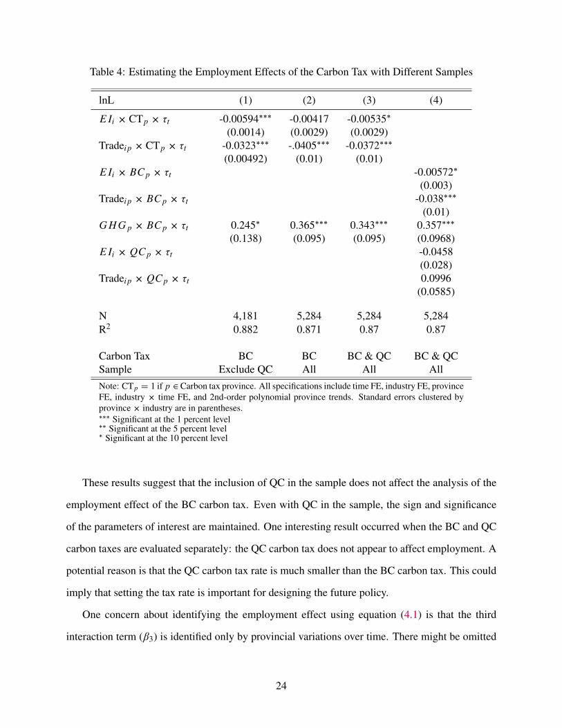
Table 4: Estimating the Employment Effects of the Carbon Tax with Different Samples
lnL (1) (2) (3) (4)
E Ii × CTp × τt -0.00594∗∗∗ -0.00417 -0.00535∗
(0.0014) (0.0029) (0.0029)Tradei p × CTp × τt -0.0323∗∗∗ -.0405∗∗∗ -0.0372∗∗∗
(0.00492) (0.01) (0.01)E Ii × BC p × τt -0.00572∗
(0.003)Tradei p × BC p × τt -0.038∗∗∗
(0.01)G H G p × BC p × τt 0.245∗ 0.365∗∗∗ 0.343∗∗∗ 0.357∗∗∗
(0.138) (0.095) (0.095) (0.0968)E Ii × QC p × τt -0.0458
(0.028)Tradei p × QC p × τt 0.0996
(0.0585)
N 4,181 5,284 5,284 5,284R2 0.882 0.871 0.87 0.87
Carbon Tax BC BC BC & QC BC & QCSample Exclude QC All All AllNote: CTp = 1 if p ∈Carbon tax province. All specifications include time FE, industry FE, provinceFE, industry × time FE, and 2nd-order polynomial province trends. Standard errors clustered byprovince × industry are in parentheses.∗∗∗ Significant at the 1 percent level∗∗ Significant at the 5 percent level∗ Significant at the 10 percent level
These results suggest that the inclusion of QC in the sample does not affect the analysis of the
employment effect of the BC carbon tax. Even with QC in the sample, the sign and significance
of the parameters of interest are maintained. One interesting result occurred when the BC and QC
carbon taxes are evaluated separately: the QC carbon tax does not appear to affect employment. A
potential reason is that the QC carbon tax rate is much smaller than the BC carbon tax. This could
imply that setting the tax rate is important for designing the future policy.
One concern about identifying the employment effect using equation (4.1) is that the third
interaction term (β3) is identified only by provincial variations over time. There might be omitted
24
variables that could contribute to the differences in employment trends between BC and the rest
of Canada. For example, employment in BC seems to be increasing in response to the carbon tax;
however, this could simply be because population (or working age population) in BC is growing
faster than the rest of Canada. Another concern is that there might be differences in job creation
and job reallocations across provinces. If workers are moving across provinces in response to
the carbon tax, this would either overstate or understate the estimation. To deal with these two
concerns, I included province- and time-varying factors in equation (4.1) as controls. The results
are reported in Table 5. These results suggest that even after taking account for potential omitted
variables, β3 is credibly identified as the point estimates stayed positive and highly significant.
25
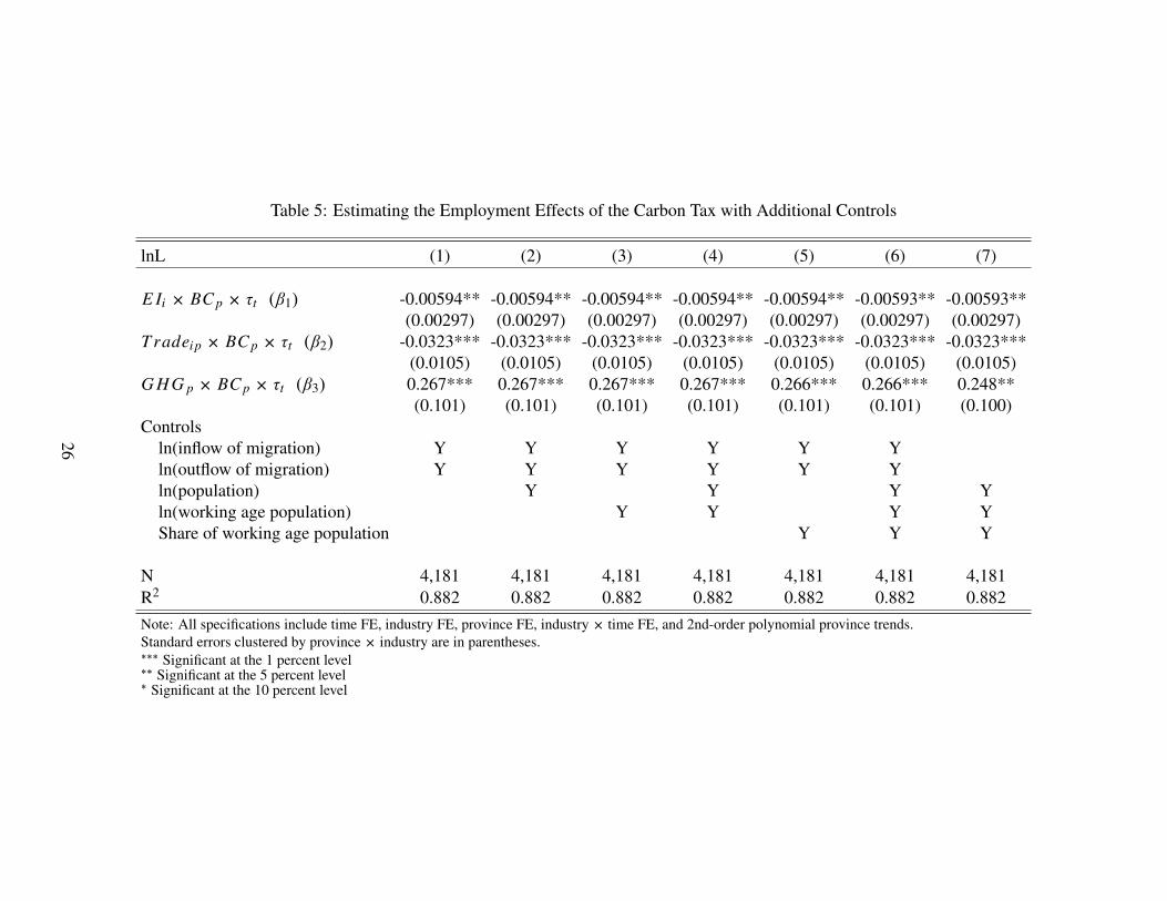
Table 5: Estimating the Employment Effects of the Carbon Tax with Additional Controls
lnL (1) (2) (3) (4) (5) (6) (7)
E Ii × BC p × τt (β1) -0.00594** -0.00594** -0.00594** -0.00594** -0.00594** -0.00593** -0.00593**(0.00297) (0.00297) (0.00297) (0.00297) (0.00297) (0.00297) (0.00297)
T radei p × BC p × τt (β2) -0.0323*** -0.0323*** -0.0323*** -0.0323*** -0.0323*** -0.0323*** -0.0323***(0.0105) (0.0105) (0.0105) (0.0105) (0.0105) (0.0105) (0.0105)
G H G p × BC p × τt (β3) 0.267*** 0.267*** 0.267*** 0.267*** 0.266*** 0.266*** 0.248**(0.101) (0.101) (0.101) (0.101) (0.101) (0.101) (0.100)
Controlsln(inflow of migration) Y Y Y Y Y Yln(outflow of migration) Y Y Y Y Y Yln(population) Y Y Y Yln(working age population) Y Y Y YShare of working age population Y Y Y
N 4,181 4,181 4,181 4,181 4,181 4,181 4,181R2 0.882 0.882 0.882 0.882 0.882 0.882 0.882Note: All specifications include time FE, industry FE, province FE, industry × time FE, and 2nd-order polynomial province trends.Standard errors clustered by province × industry are in parentheses.∗∗∗ Significant at the 1 percent level∗∗ Significant at the 5 percent level∗ Significant at the 10 percent level
26
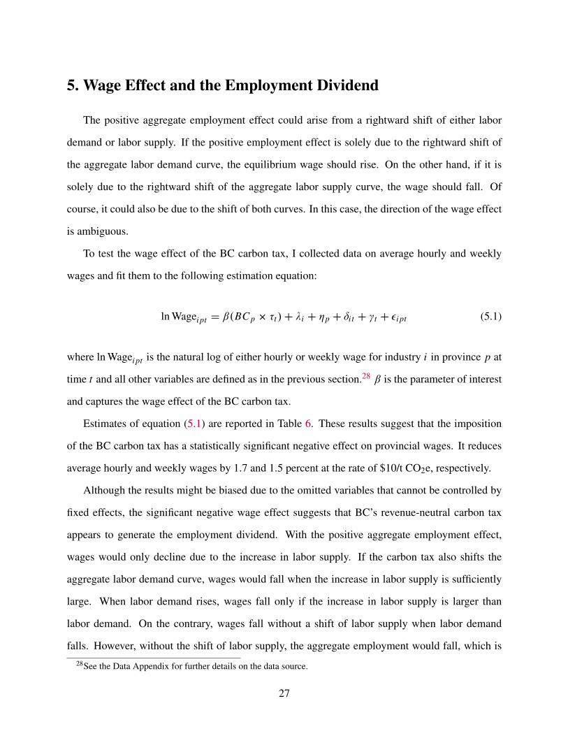
5. Wage Effect and the Employment Dividend
The positive aggregate employment effect could arise from a rightward shift of either labor
demand or labor supply. If the positive employment effect is solely due to the rightward shift of
the aggregate labor demand curve, the equilibrium wage should rise. On the other hand, if it is
solely due to the rightward shift of the aggregate labor supply curve, the wage should fall. Of
course, it could also be due to the shift of both curves. In this case, the direction of the wage effect
is ambiguous.
To test the wage effect of the BC carbon tax, I collected data on average hourly and weekly
wages and fit them to the following estimation equation:
ln Wagei pt = β(BC p × τt)+ λi + ηp + δi t + γt + εi pt (5.1)
where ln Wagei pt is the natural log of either hourly or weekly wage for industry i in province p at
time t and all other variables are defined as in the previous section.28 β is the parameter of interest
and captures the wage effect of the BC carbon tax.
Estimates of equation (5.1) are reported in Table 6. These results suggest that the imposition
of the BC carbon tax has a statistically significant negative effect on provincial wages. It reduces
average hourly and weekly wages by 1.7 and 1.5 percent at the rate of $10/t CO2e, respectively.
Although the results might be biased due to the omitted variables that cannot be controlled by
fixed effects, the significant negative wage effect suggests that BC’s revenue-neutral carbon tax
appears to generate the employment dividend. With the positive aggregate employment effect,
wages would only decline due to the increase in labor supply. If the carbon tax also shifts the
aggregate labor demand curve, wages would fall when the increase in labor supply is sufficiently
large. When labor demand rises, wages fall only if the increase in labor supply is larger than
labor demand. On the contrary, wages fall without a shift of labor supply when labor demand
falls. However, without the shift of labor supply, the aggregate employment would fall, which is28See the Data Appendix for further details on the data source.
27
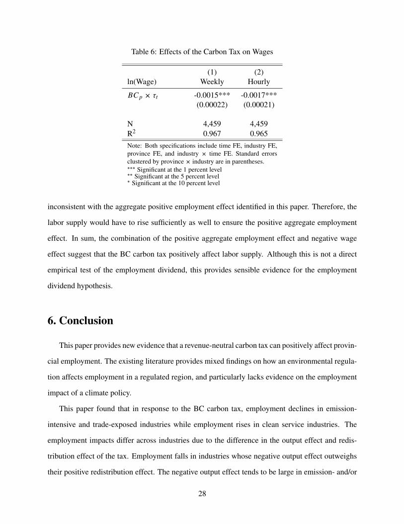
Table 6: Effects of the Carbon Tax on Wages
(1) (2)ln(Wage) Weekly Hourly
BC p × τt -0.0015*** -0.0017***(0.00022) (0.00021)
N 4,459 4,459R2 0.967 0.965Note: Both specifications include time FE, industry FE,province FE, and industry × time FE. Standard errorsclustered by province × industry are in parentheses.∗∗∗ Significant at the 1 percent level∗∗ Significant at the 5 percent level∗ Significant at the 10 percent level
inconsistent with the aggregate positive employment effect identified in this paper. Therefore, the
labor supply would have to rise sufficiently as well to ensure the positive aggregate employment
effect. In sum, the combination of the positive aggregate employment effect and negative wage
effect suggest that the BC carbon tax positively affect labor supply. Although this is not a direct
empirical test of the employment dividend, this provides sensible evidence for the employment
dividend hypothesis.
6. Conclusion
This paper provides new evidence that a revenue-neutral carbon tax can positively affect provin-
cial employment. The existing literature provides mixed findings on how an environmental regula-
tion affects employment in a regulated region, and particularly lacks evidence on the employment
impact of a climate policy.
This paper found that in response to the BC carbon tax, employment declines in emission-
intensive and trade-exposed industries while employment rises in clean service industries. The
employment impacts differ across industries due to the difference in the output effect and redis-
tribution effect of the tax. Employment falls in industries whose negative output effect outweighs
their positive redistribution effect. The negative output effect tends to be large in emission- and/or
28
trade-intensive industries, resulting in the negative employment effect.
By aggregating the employment effects across industries, the overall employment effect of the
BC carbon tax appears to be positive. The positive employment effects outweighs the negative
employment effects because labor-intensive industries experience job gains. The results from the
preferred specification suggests that the implementation of the BC carbon tax explains 40 percent
of the observed increase in BC’s employment over the 2007-2013 period. To put this into context,
the BC carbon tax generated a small but statistically significant 2 percent increase in employment
over these six years, an average of 5,000 jobs annually.
I also investigated the effect of the BC carbon tax on provincial wages, and found that the
tax had a statistically significant negative effect. This suggests that the increase in aggregate em-
ployment partly comes from the rightward shift of labor supply, which provides support for the
employment dividend hypothesis.
Although these estimates are not outcomes of randomized experiments, they provide fairly
robust evidence that a revenue-neutral carbon tax does not adversely affect employment in a reg-
ulated region. The latest report (Elgie and McClay, 2013) claimed that the implementation of the
carbon tax did not have any apparent adverse impact on BC’s economy. This paper adds another
perspective to the evaluation of the BC carbon tax because the report only focused on the impact to
BC’s GDP. To my knowledge, this paper is the first to provide the ex post empirical evaluation of a
revenue neutral carbon tax. As the structure of a carbon tax can take many different forms in terms
of the rate, the coverage of tax-base, and the treatment of the tax revenue, empirical investigations
of a carbon tax in other regions would bring fruitful contributions to the literature.
29
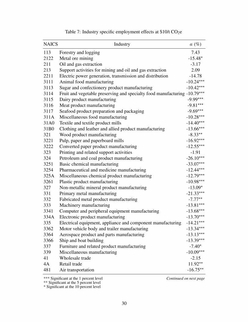
Table 7: Industry specific employment effects at $10/t CO2e
NAICS Industry α (%)
113 Forestry and logging 7.432122 Metal ore mining -15.48∗
211 Oil and gas extraction -3.17213 Support activities for mining and oil and gas extraction 2.092211 Electric power generation, transmission and distribution -14.783111 Animal food manufacturing -10.24∗∗∗
3113 Sugar and confectionery product manufacturing -10.42∗∗∗
3114 Fruit and vegetable preserving and specialty food manufacturing -10.79∗∗∗
3115 Dairy product manufacturing -9.99∗∗∗
3116 Meat product manufacturing -9.81∗∗∗
3117 Seafood product preparation and packaging -9.69∗∗∗
311A Miscellaneous food manufacturing -10.28∗∗∗
31A0 Textile and textile product mills -14.40∗∗∗
31B0 Clothing and leather and allied product manufacturing -13.66∗∗∗
321 Wood product manufacturing -8.33∗∗
3221 Pulp, paper and paperboard mills -16.92∗∗∗
3222 Converted paper product manufacturing -12.55∗∗∗
323 Printing and related support activities -1.91324 Petroleum and coal product manufacturing -26.10∗∗∗
3251 Basic chemical manufacturing -33.07∗∗∗
3254 Pharmaceutical and medicine manufacturing -12.44∗∗∗
325A Miscellaneous chemical product manufacturing -12.79∗∗∗
3261 Plastic product manufacturing -10.98∗∗∗
327 Non-metallic mineral product manufacturing -13.09∗
331 Primary metal manufacturing -21.33∗∗∗
332 Fabricated metal product manufacturing -7.77∗∗
333 Machinery manufacturing -13.81∗∗∗
3341 Computer and peripheral equipment manufacturing -13.68∗∗∗
334A Electronic product manufacturing -13.70∗∗∗
335 Electrical equipment, appliance and component manufacturing -14.21∗∗∗
3362 Motor vehicle body and trailer manufacturing -13.34∗∗∗
3364 Aerospace product and parts manufacturing -13.13∗∗∗
3366 Ship and boat building -13.39∗∗∗
337 Furniture and related product manufacturing -7.40∗
339 Miscellaneous manufacturing -10.09∗∗∗
41 Wholesale trade -2.154A Retail trade 11.92∗∗
481 Air transportation -16.75∗∗
*** Significant at the 1 percent level Continued on next page** Significant at the 5 percent level* Significant at the 10 percent level
30
NAICS Industry α (%)
482 Rail transportation -5.18484 Truck transportation -8.97∗
48B0 Transit, ground, scenic and sightseeing passenger transportation -0.85493 Warehousing and storage 0.2151 Information and cultural industries -1.515A01 Depository credit intermediation and monetary authorities 4.815241 Insurance carriers 6.185A06 Other finance, insurance and real estate 5.725311 Lessors of real estate 11.43∗
5A05 Rental and leasing services 12.33∗∗
541 Professional, scientific and technical services 4.56561 Administrative and support services 4.52562 Waste management and remediation services 2.036113 Universities 8.76∗
611A Educational services (except universities) 8.51∗
622 Hospitals 16.13∗∗∗
62A0 Health care services (except hospitals) and social assistance 16.19∗∗∗
71 Arts, entertainment and recreation 0.9372 Accommodation and food services 0.63
*** Significant at the 1 percent level** Significant at the 5 percent level* Significant at the 10 percent level
31
Basic chemical manufacturingPetroleum and coal product manufacturing
Primary metal manufacturingPulp, paper and paperboard mills
Air transportationMetal ore mining
Electric power generation, transmission and distributionTextile and textile product mills
Electrical equipment, appliance and component manufacturingMachinery manufacturing
Electronic product manufacturingComputer and peripheral equipment manufacturing
Clothing and leather and allied product manufacturingShip and boat building
Motor vehicle body and trailer manufacturingAerospace product and parts manufacturingNon-metallic mineral product manufacturing
Miscellaneous chemical product manufacturingConverted paper product manufacturing
Pharmaceutical and medicine manufacturingPlastic product manufacturing
Fruit and vegetable preserving and specialty food manufacturingSugar and confectionery product manufacturing
Miscellaneous food manufacturingAnimal food manufacturing
Miscellaneous manufacturingDairy product manufacturingMeat product manufacturing
Seafood product preparation and packagingTruck transportation
Wood product manufacturingFabricated metal product manufacturing
Furniture and related product manufacturingRail transportation
Oil and gas extractionWholesale trade
Printing and related support activitiesInformation and cultural industries
Transit, ground, scenic and sightseeing passenger transportationWarehousing and storage
Accommodation and food servicesArts, entertainment and recreation
Waste management and remediation servicesSupport activities for mining and oil and gas extraction
Administrative and support servicesProfessional, scientific and technical services
Depository credit intermediation and monetary authoritiesOther finance, insurance and real estate and management of companies
Insurance carriersForestry and logging
Educational services (except universities)Universities
Lessors of real estateRetail trade
Rental and leasing services and lessors of non-financial intangible associationsHospitals
Health care services (except hospitals) and social assistance
-50 -40 -30 -20 -10 0 10 20 30
Change in Employment (%)
Figure 8: Industry Specific Employment Effects with 95% C.I.
Source: Author’s calculation
32
Basic chemical manufacturingPetroleum and coal product manufacturing
Primary metal manufacturingPulp, paper and paperboard mills
Air transportationElectric power generation, transmission and distribution
Textile and textile product millsElectrical equipment, appliance and component manufacturing
Machinery manufacturingComputer and peripheral equipment manufacturing
Clothing and leather and allied product manufacturingShip and boat building
Motor vehicle body and trailer manufacturingAerospace product and parts manufacturingNon-metallic mineral product manufacturing
Converted paper product manufacturingPharmaceutical and medicine manufacturing
Fruit and vegetable preserving and specialty food manufacturingSugar and confectionery product manufacturing
Miscellaneous food manufacturingAnimal food manufacturing
Miscellaneous manufacturingDairy product manufacturingMeat product manufacturing
Seafood product preparation and packagingTruck transportation
Wood product manufacturingFabricated metal product manufacturing
Furniture and related product manufacturingRail transportation
Oil and gas extractionWholesale trade
Printing and related support activitiesInformation and cultural industries
Transit, ground, scenic and sightseeing passenger transportationWarehousing and storage
Accommodation and food servicesArts, entertainment and recreation
Waste management and remediation servicesSupport activities for mining and oil and gas extraction
Administrative and support servicesProfessional, scientific and technical services
Depository credit intermediation and monetary authoritiesOther finance, insurance and real estate and management of companies
Insurance carriersForestry and logging
Educational services (except universities)Universities
Lessors of real estateRetail trade
Rental and leasing services and lessors of non-financial intangible associationsHospitals
Health care services (except hospitals) and social assistance
-5 0 5 10 15 20 25 30
Changes in Employment (in thousands)
Figure 9: Changes in Employment at $10/t CO2e
Source: Author’s calculation
33
ReferencesBerman, Eli, and Linda T.M Bui. 2001. “Environmental regulation and labor demand: evidence
from the South Coast Air Basin.” Journal of Public Economics, 79(2): 265–295.
Bezdek, Roger H., Robert M. Wendling, and Jonathan D. Jones. 1989. “The economic andemployment effects of investments in pollution abatement and control technologies.” Ambio,18(5): 274–279.
Bosquet, Benoit. 2000. “Environmental tax reform: does it work? A survey of the empiricalevidence.” Ecological economics, 34: 19–32.
Bovenberg, A.Lans, and Lawrence H. Goulder. 2002. “Environmental Taxation and Regula-tion.” Handbook of Public Economics, 3: 1471–1545.
Boyle, Matthew. 2011. “EPA regulation forces closure of Texas energy facilities, eliminates 500jobs.” The Daily Caller.
Brimblecombe, Peter. 2006. “The Clean Air Act after 50 years.” Weather, 61(11): 311–314.
Cama, Timothy. 2015. “Coal company lays off hundreds, blames Obama policies.” The Hill.
Carraro, Carlo, Marzio Galeotti, and Massimo Gallo. 1996. “Environmental Taxation and un-employment: Some Evidence on the ’Double Dividend Hypothesis’ in Europe.” Journal of Pub-lic Economics, 62: 141–181.
Duff, David G. 2008. “Carbon Taxation in British Columbia.” Vermont Journal of EnvironmentalLaw, 10: 87–108.
Elgie, Stewart, and Jessica McClay. 2013. “BCs Carbon Tax Shift Is Working Well after FourYears (Attention Ottawa).” Canadian Public Policy, 39(s2): S1–S10.
Environmental Canada. 2011. “Summary of B.C. Greenhouse Gas Emissions: 1990-2011 (kilo-tonnes CO2e).”
Environmental Protection Agency. 1981. “The Macroeconomic Impact of Federal PollutionControl Programs–1981 Assessment.” The Environmental Protection Agency Data Resources,Inc.
Greenstone, Michael. 2002. “The Impacts of Environmental Regulations on Industrial Activity :Evidence from the 1970 and 1977 Clean Air Act Amendments and the Census of Manufactures.”Journal of Political Economy, 110(6): 1175–1219.
Grenoble, Ryan. 2013. “Green Job Growth Outpaced All Other Industries 2010-2011.” The Huff-ington Post2.
Harrison, Kathryn. 2012. “A tale of two taxes: The fate of environmental tax reform in Canada.”Review of Policy Research, 29(3): 383–407.
34
Hazilla, Michael, and R J Kopp. 1990. “Social cost of environmental quality regulations: Ageneral equilibrium analysis.” Journal of Political Economy, 98(4): 853–873.
Hollenbeck, Kevin. 1979. “The employment and earnings impacts of the regulation of stationarysource air pollution.” Journal of Environmental Economics and Management, 6: 208–221.
Kotlikoff, Laurent J., and Lawrence H. Summer. 1987. “Tax Incidence.” In Handbook of Pub-lic Economics. . 2 ed., , ed. Alan J. Auerbach and Martin Feldstein, Chapter 16, 1043–1092.Amsterdam:Elsevier Science.
Majocchi, Alberto. 1996. “Green fiscal reform and employment: A survey.” Environmental &Resource Economics, 8: 375–397.
Martin, Ralf, Laure B. de Preux, and Ulrich J. Wagner. 2014. “The impact of a carbon tax onmanufacturing: Evidence from microdata.” Journal of Public Economics, 117: 1–14.
Ministry of Finance. 2008. “Budget and Fiscal Plan 2008/09-2010/11.” British Columbia.
Ministry of Finance. 2013. “Budget and Fiscal Plan 2013/14-2015/16.” British Columbia.
Ministry of Finance. 2014. “Budget and Fiscal Plan 2014/15-2016/17.” British Columbia.
Morgenstern, Richard D. 2010. “The Potential Impact on Energy-Intensive Trade-Exposed In-dustries of Clean Air Act Regulation of GHGs.”
Nunn, Nathan, and Nancy Qian. 2011. “The potato’s contribution to population and urbanization:Evidence from a historical experiment.” Quarterly Journal of Economics, 126(2): 593–650.
Rivers, Nicholas, and Brandon Schaufele. 2014. “The Effect of Carbon Taxes on AgriculturalTrade.” Canadian Journal of Agricultural Economics, 00: 1–23.
Statistics Canada. 2012. “Table 153-0034 - Greenhouse gas emissions (carbon dioxide equiva-lents), by sector, annual (kilotonnes).”
Statistics Canada. 2014a. “Table 281-0024 - Survey of Employment, Payrolls and Hours (SEPH),employment by type of employee and detailed North American Industry Classification System(NAICS).”
Statistics Canada. 2014b. “Table 379-0029 - Gross domestic product (GDP) at basic prices, byNorth American Industry Classification System (NAICS), annual (dollars).”
Statistics Canada. 2014c. “Table 386-0003 - Provincial input-output tables, international and in-terprovincial trade flows, summary level, basic prices, annual (dollars).”
United Nations Environment Programme. 2008. “Green Jobs: towards decent work in a sustain-able, low-carbon world.”
US EPA. 2013. “History of the Clean Air Act.”
Wendling, Robert M., and Roger H. Bezdek. 1989. “Acid rain abatement legislationCosts andbenefits.” Omega, 17(3): 251–261.
35
A. Data Appendix
This appendix describes additional details of the data sources and construction used to cre-
ate the dataset for the analysis. It also provides a list of industries in the sample as well as the
concordance between two classifications.
I. Data
To identify the employment effect of the BC carbon tax, I collected data on employment (Table
281-0024), GHG emission intensity (Table 153-0034 and 379-0029), and trade intensity (Table
386-0003) from tables in Statistics Canada.
Employment is measured as a number of all employees in an industry. GHG emission in-
tensity is calculated as GHG emission (Table 153-0034) divided by industrial GDP (Table 379-
0029) and measured in tonnes per thousand dollars of production. Trade intensity is defined as
(Import + Export)/(Total demand + Import). Import and export both include international and
inter-provincial trade. Total demand is defined as the sum of consumption out of own production
and inventory withdrawals plus exports. This construction of trade intensity is to have a similar
meaning to openness to trade, which is often calculated as (Import+ Export)/GDP.
Although all these variables are obtained from Statistics Canada, they are categorized based on
the different classifications. Employment and emission intensity data are categorized based on the
North American Industry Classification System (NAICS) while trade intensity data is categorized
based on the North American Products Classification System (NAPCS). As Statistics Canada pro-
vides the detail description for each category of the classifications, manual merging is possible to
construct the dataset for this analysis. The concordance between these classifications is listed in
the next section.
I also collected data on wage to identify the wage effect of the BC carbon tax. Average hourly
and weekly wage data are obtained from Table 282-0072 in Statistics Canada. They are measured
in current dollar and categorized based on NAICS.
36
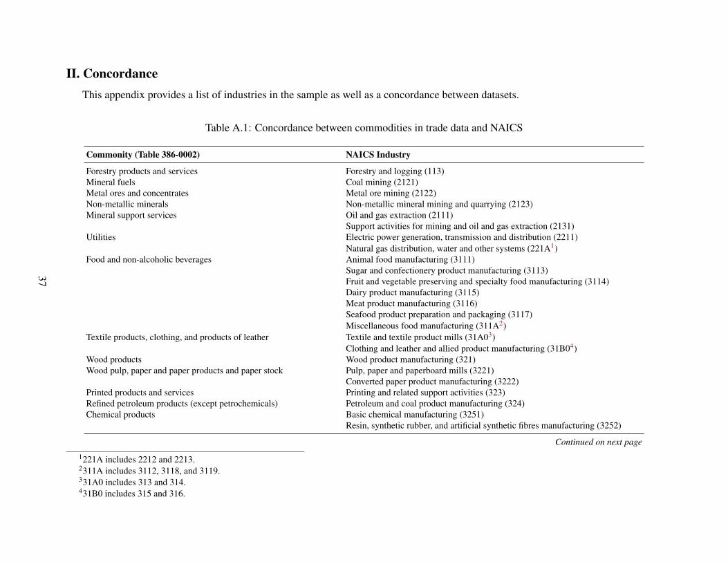
II. ConcordanceThis appendix provides a list of industries in the sample as well as a concordance between datasets.
Table A.1: Concordance between commodities in trade data and NAICS
Commonity (Table 386-0002) NAICS Industry
Forestry products and services Forestry and logging (113)Mineral fuels Coal mining (2121)Metal ores and concentrates Metal ore mining (2122)Non-metallic minerals Non-metallic mineral mining and quarrying (2123)Mineral support services Oil and gas extraction (2111)
Support activities for mining and oil and gas extraction (2131)Utilities Electric power generation, transmission and distribution (2211)
Natural gas distribution, water and other systems (221A1)Food and non-alcoholic beverages Animal food manufacturing (3111)
Sugar and confectionery product manufacturing (3113)Fruit and vegetable preserving and specialty food manufacturing (3114)Dairy product manufacturing (3115)Meat product manufacturing (3116)Seafood product preparation and packaging (3117)Miscellaneous food manufacturing (311A2)
Textile products, clothing, and products of leather Textile and textile product mills (31A03)Clothing and leather and allied product manufacturing (31B04)
Wood products Wood product manufacturing (321)Wood pulp, paper and paper products and paper stock Pulp, paper and paperboard mills (3221)
Converted paper product manufacturing (3222)Printed products and services Printing and related support activities (323)Refined petroleum products (except petrochemicals) Petroleum and coal product manufacturing (324)Chemical products Basic chemical manufacturing (3251)
Resin, synthetic rubber, and artificial synthetic fibres manufacturing (3252)
Continued on next page
1221A includes 2212 and 2213.2311A includes 3112, 3118, and 3119.331A0 includes 313 and 314.431B0 includes 315 and 316.
37
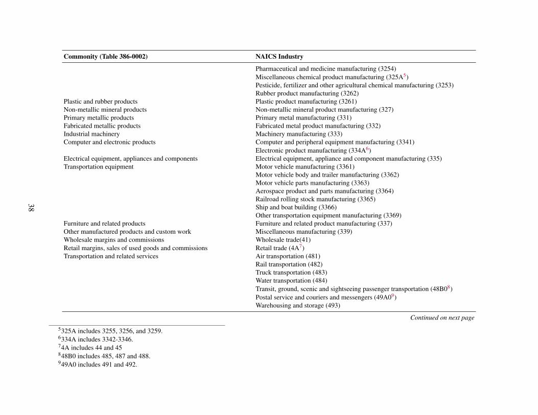
Commonity (Table 386-0002) NAICS Industry
Pharmaceutical and medicine manufacturing (3254)Miscellaneous chemical product manufacturing (325A5)Pesticide, fertilizer and other agricultural chemical manufacturing (3253)Rubber product manufacturing (3262)
Plastic and rubber products Plastic product manufacturing (3261)Non-metallic mineral products Non-metallic mineral product manufacturing (327)Primary metallic products Primary metal manufacturing (331)Fabricated metallic products Fabricated metal product manufacturing (332)Industrial machinery Machinery manufacturing (333)Computer and electronic products Computer and peripheral equipment manufacturing (3341)
Electronic product manufacturing (334A6)Electrical equipment, appliances and components Electrical equipment, appliance and component manufacturing (335)Transportation equipment Motor vehicle manufacturing (3361)
Motor vehicle body and trailer manufacturing (3362)Motor vehicle parts manufacturing (3363)Aerospace product and parts manufacturing (3364)Railroad rolling stock manufacturing (3365)Ship and boat building (3366)Other transportation equipment manufacturing (3369)
Furniture and related products Furniture and related product manufacturing (337)Other manufactured products and custom work Miscellaneous manufacturing (339)Wholesale margins and commissions Wholesale trade(41)Retail margins, sales of used goods and commissions Retail trade (4A7)Transportation and related services Air transportation (481)
Rail transportation (482)Truck transportation (483)Water transportation (484)Transit, ground, scenic and sightseeing passenger transportation (48B08)Postal service and couriers and messengers (49A09)Warehousing and storage (493)
Continued on next page
5325A includes 3255, 3256, and 3259.6334A includes 3342-3346.74A includes 44 and 45848B0 includes 485, 487 and 488.949A0 includes 491 and 492.
38
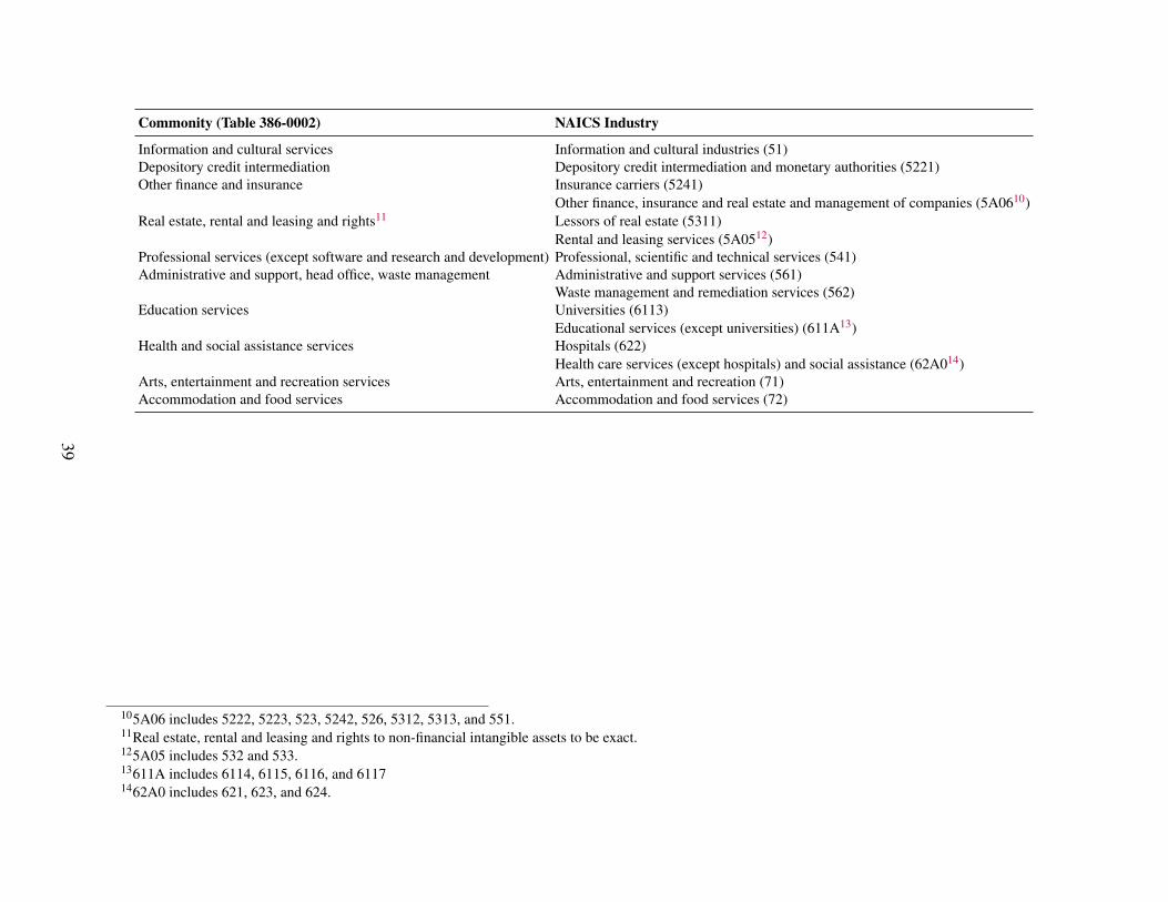
Commonity (Table 386-0002) NAICS Industry
Information and cultural services Information and cultural industries (51)Depository credit intermediation Depository credit intermediation and monetary authorities (5221)Other finance and insurance Insurance carriers (5241)
Other finance, insurance and real estate and management of companies (5A0610)Real estate, rental and leasing and rights11 Lessors of real estate (5311)
Rental and leasing services (5A0512)Professional services (except software and research and development) Professional, scientific and technical services (541)Administrative and support, head office, waste management Administrative and support services (561)
Waste management and remediation services (562)Education services Universities (6113)
Educational services (except universities) (611A13)Health and social assistance services Hospitals (622)
Health care services (except hospitals) and social assistance (62A014)Arts, entertainment and recreation services Arts, entertainment and recreation (71)Accommodation and food services Accommodation and food services (72)
105A06 includes 5222, 5223, 523, 5242, 526, 5312, 5313, and 551.11Real estate, rental and leasing and rights to non-financial intangible assets to be exact.125A05 includes 532 and 533.13611A includes 6114, 6115, 6116, and 61171462A0 includes 621, 623, and 624.
39