1

GOVERNMENT DOCTOR ABSENTEEISM AND ITS EFFECTS ON

CONSUMER DEMAND IN RURAL NORTH INDIA.

Richard A. Iles1

Job Market Paper

Abstract

Counterfactual demand estimation is useful means of evaluating the efficacy of improving the

supply of government doctors in low-income settings. Joint modelling of revealed and stated

preference data provides a counterfactual context for outpatient fever treatment demand

estimation, under the assumption of full availability of qualified government doctors. The

demand framework presented investigates the interrelationship between government doctor

absenteeism and the large outpatient healthcare market share held by the informal sector.

Modelling incorporates healthcare provider quality via the use of a qualitative measure of

word-of-mouth recommendations. Results support the hypothesis that consumers perceive

unqualified provider services as being of lower quality.

1 XXXX richard.iles@griffithuni.edu.au. This research was supported by a Ph.D scholarship from Griffith

University (Australia) and the Centre for Development Economics – Delhi School of Economics (India) who

hosted the author as a Visiting Scholar in 2012.

2

The human development benefits of access to affordable and high quality healthcare, among

other thing, help motivate policy-makers to consider the introduction of universal healthcare

(Stuckler et al., 2010). High levels of out-of-pocket healthcare expenditure are common in

developing economy health systems (World databank, 2015). However, the impact of

introducing subsidised healthcare, which is a pervasive element of universal healthcare

models, and as a consequence reduce healthcare related impoverishment, depend in part, on

consumer preferences and the universal healthcare design. In contexts where the informal

sector operates widely, understanding consumer preferences and demand is particularly

important to ensure possible universal healthcare models are effective (Mebratic et al., 2015;

see Böhme and Thiele, 2012 and Banerjee and Jain, 2007 for informal sector). Estimating

consumer demand across a full range of formal and informal allopathic2 healthcare providers,

affords valuable insights into developing economies’ outpatient healthcare markets.

The complexity of introducing universal healthcare in developing economies is extenuated by

widespread variations in healthcare provider quality. Pluralistic and heterogeneous health

market reflects the varied primary healthcare provider quality found within developing

economies (Pinto, 2004). Das et al. (2012) identified that private qualified providers in north

India offered the highest clinical quality outpatient care, followed by government qualified

and private unqualified providers. However, of particular interest was that private unqualified

providers did not perform significantly worse than qualified government providers when

quality was measured by providers use of correct treatments, as opposed to diagnostic

questions.In these markets qualified and unqualified providers often operate alongside one

another (Chang and Trivedi, 2003; Das and Hammer, 2007; Das et al., 2012), prices of

private and government providers are effectively unregulated (Ensor, 2004; Mæstad and

Mwisongo, 2011) and consumers are forced to make provider choices based on limited

clinical quality related information (Das and Das, 2003).

Limited supply of qualified doctors in rural areas is a widespread problem that reduces

consumers’ acceass to high quality healthcare. A range of government incentives is used to

induce young doctors to practice in rural communities (Dussault and Franceschini, 2006;

Holte et al., 2015). In developing economies, the under-supply of qualified doctors is

2Allopathic medicine is a term used to refer to ‘western’ medicine. This is in contrast to traditional Indian

systems of medicine.

3

exacerbated by government doctor absenteeism and the prevalence of doctor dual practice in

the public and private sectors (Vujicic et al., 2010 for under-supply of doctors; Banerjee et

al., 2004 and Chaudhury et al., 2006 on absenteeism; Hipgrave and Hort, 2014; Mcpake et

al., 2014 on dual practice). Concurrent with government doctor absenteeism, limited

available data indicates the widespread prevalence of informal private healthcare providers.

In India the estimated percentage of informal doctors of all available healthcare providers is

between 45-80 per cent (MAQARI Team, 2011; The WorldBank, 1998). By contrast

utilisation of government outpatient care is estimated between 20 to 30 per cent in India

(NSSO, 2015).

Healthcare quality is an important component in the derived demand for healthcare.

Grossman’s demand for health model (1972) has quality (as measured by the ratio of the time

to restore health (T) over a quantity of medical care consumed (M)) as a central component

driving consumers’ health investment decisions. Early empirical work in the United States

made various attempts to incorporate healthcare quality in demand estimations (Colle and

Grossman, 1978; Goldman and Grossman, 1978). Later empirical work in developing

economies provider quality was allowed to drop out of a reduced form random utility model

(Gertler et al., 1987; Sahn et al., 2003). However, the demand framework developed by

Chang and Trivedi (2003) modelled healthcare quality as a random component.

Consumer trust in healthcare providers and institutions are well established as an important

qualitative factor affecting perceived quality and consumer choice (Ager et al., 2005; Das and

Das, 2003; Ozawa and Walker, 2011; Russell, 2005). Among consumers with relatively low

levels of literacy word-of-mouth recommendations are common information channels

through which they evaluate the relative quality of available outpatient healthcare providers

(Ahmed et al., 2014). Results from rural Tanzania indicate that consumers value positive and

negative recommendations differently depending on their familiarity with a given provider

(Leonard et al., 2009).

This article addresses the question of how important is doctor absenteeism in explaining the

low level of utilisation of public sector outpatient healthcare services in rural Uttar Pradesh,

India. In so doing, a range of behavioural qualitative variables is incorporated into consumer

demand estimates. These include: i) word-of-mouth recommendations, ii) perceived quality

4

of mode of medicine administration and generic government medicines (Basak and

Sathyanarayana, 2012), and iii) the perceived need to make payments (either informal or to

private chemists) for medicines prescribed by government doctors (see Appendix A for a

summary of perceived reasons for non-use of government doctors from the sample data). As

a result, new insights into consumer decision-making behaviour are provided that indicate

that consumers are aware of quality differences between qualified and unqualified providers.

Consumer demand estimates presented here reflects a range of actual and counterfactual3

scenarios available in villages and their surrounds. This article incorporates a qualitative

measure of healthcare provider quality via the use of stated choice (SC) data in joint revealed

and stated preference demand estimation. The criticism of counterfactual analysis offered by

Elster (1978) “…that the choice of counterfactuals ex-post is often guided by the range of

subjective opinions open to the actors ex-ante” (p.180) is not believed to be relevant in this

analysis. The fact that government doctor absenteeism is a breaking of labour contracts the

assumed scenario that doctors are fully present at their allocated posts is reasonable.

The utility framework and functional form used are outlined in Section 1, the joint revealed

and stated preference modelling is explained in Section 2, while Section 3 provides a

description of the data. Sections 4 and 5 contain the demand estimation results and the

associated price elasticity.

3 According to McCloskey (1987) the use of counterfactual is one of several paradigms commonly used by

economists to “explore the world”. The two general problems, as identified by McCloskey, with the use of

counterfactual scenarios – vagueness and absurdity – are not believed to be present in the current application.

The assumption that government employees are present at their nominated posts is neither vague nor absurd.

5

1. Economic Model

Estimation of unconditional demand using revealed preference (RP) and SC data draws on

the same systematic, stochastic utility structure. The systematic component of the random

utility model, used in this article, is non-linear in parameters and linear in the attributes. The

log of household income enters the function twice, with the second entry is as a squared term.

This allows for the testing of the convexity of the relationship between income and health.

Prices enter the utility function independently of income. Despite earlier concerns about the

lack of stability in utility maximisation estimates due to independent price parameters

(Gertler et al., 1987), more recent work demonstrates that stability is maintained with the

inclusion of price parameters (Dow, 1995). The deterministic component of the random

utility function for the modelis given below

𝑉𝑞𝑞𝑞𝑞 = 𝛽0 + 𝜷1′ 𝑿𝑞 + 𝜷2′ 𝒁𝑞 + 𝛼1 ln(𝑌) + 𝛼2 ln(𝑌)2 + 𝛼3𝑃𝑞

+𝜷3′𝑾𝑞 + 𝜷4′ 𝑮𝑞 + 𝜷5′ 𝑫𝑞 + u, (1)

where subscripts q, j, k, m denote consumers, provider alternatives, government provider

specific factors and unqualified provider factors. The vectors X and Z represent consumer and

healthcare provider characteristics. These include: caste, literacy level, employment category

and travel distance. The vectors W, G and D relate to perceived provider quality, government

and unqualified specific determinants. Previous related work usingconditional choice data

and Multinomial Logit (MNL) and Latent Class MNL models, shows statistical significance

of the qualitative variables: positive and negative recommendations, extra charge for

government medicines (i.e. informal patient payments) and mode of fever treatment by

unqualified – jhola chhaap4 – provider (Iles and Rose, 2014).

4The Hindi phrase jhola chhaap is used to refer to unqualified allopathic healthcare providers (Willis et al.,

2011). It carries negative connotations. As a result it may be likened to the term ‘quack’. However, due to the

terms use in data collection and respondents’ use of this term as a point of reference in answering questions, the

term is repeated throughout the paper to avoid confusion with other methods of defining unqualified allopathic

providers in India.

6

2. Model Estimation

Modelling consumer demand using recall-based survey data (i.e. revealed preference) and SC

data (i.e. stated preference) assists by adding behavioural insight with market realism.

Demand estimation using both data is desirable in the context of: i) seeking to incorporate

qualitative behavioural and product attributes, and ii) limited information about the market

characteristics of non-selected alternatives. The absence of full information about all

available primary healthcare market alternatives in treating fevers in rural north India

requires the maximising of second-best data alternatives. The imputation of supply-side

information about non-selected market alternatives is a common means of overcoming the

data limitation often encountered when relying on recall-based survey data (Ben-Akiva and

Lerman, 1985; Borah, 2006). Moreover, the incorporation of derived price and qualitative

variable parameter estimates, which are based on trade-offs with market alternatives, provide

a mapping of conference preferences. This data may help to limit potential biases due to the

use of imputed product attributes as the basis of consumer trade-offs.

Consumer demand estimates for types of healthcare providers in developing economies has

widely utilised Maximum Likelihood estimators for qualitative response data. The Random

Parameter Logit (RPL) model extends standard Multinomial Logit (MNL) estimations by

introducing β estimates that vary across individuals. The greater flexibility of the RPL also

carries favourable behavioural characteristics. The standard deviations of βqj denote

unobserved preference heterogeneity across sub-sets of individuals. The parameter estimate

for the random variable βqj of individual q and healthcare provider j, can be decomposed as

𝛃𝑞𝑞 = 𝛃𝑞 + 𝜹𝑞′w𝑞 + 𝛈𝑞𝑞, j=1,2,3,4

with 𝛈𝑞𝑞 = 𝛔𝑞𝒗𝑞𝑞. The vector wq is observed data. The vector vqj contains the unobserved

random residuals. The inclusion of the term 𝛈𝑞𝑞 allows for correlation in the error terms

across choices.

The mixing of distributions in the RPL is a distinguishing feature of the model. The term 𝛈𝑞𝑞

can take a number of general distributions (i.e. normal, log-normal and exponential) with the

error term continuing to take the IID distribution. The combination of different distributions

in the model gives rise to a joint distribution 𝑓�𝜼𝒒�w𝑞,Ξ), where Ξ denotes the parameters of

7

the distribution of wq for observed data. The RPL model contains: i) conditional elements of

the simulated Maximum Likelihood given in (4) and ii) the joint distribution mixing function.

The conditional element of the RPL equation retains the ratio of probabilities established the

base MNL,

L𝑞𝑞�β𝑞�X𝑞,η𝒒� = 𝑒x𝑞𝑞′ β𝑞𝑞

∑ 𝑒x𝑞𝑞′ β𝑞𝑞𝐽

𝑞=1

. (4)

The unconditional probability of the RPL, on which the simulated Maximum Likelihood is

run is given in equation (5) and includes parts i) and ii) outlined above. This more flexible

multi-choice model has received recent support within the healthcare demand literature for its

ability to relax the IID assumption and more accurately capture unobserved heterogeneity

(Borah, 2006; Erlyana et al., 2011; Meenakshi et al., 2012; Qian et al., 2009),

𝑃𝑞𝑞�𝑿𝒒, z𝒒,Ξ� = ∫ 𝐿𝑞𝑞�𝜷𝒒�𝑿𝑞 ,𝜼𝒒) 𝑓�𝜼𝒒�w𝑞,Ξ�𝑑𝜼𝒒.𝛽𝑞 (5)

The inclusion of error components to RPL is one way of accounting for the differences in

error variance. Such a modelling approach enables four important issues to be adequately

managed when modelling RP-SP data jointly: i) error structure, ii) scale difference, iii)

unobserved heterogeneity effects and iv) state-dependence effects (Bhat and Castelar, 2002).

Error Components (EC) are a set of independent individual terms that are added to the utility

function. The non-IID error structure is maintained in the RPL (EC) from the base RPL

model. The unified RP-SP modelling approach of Bhat and Castelar (2002) as established a

modelling practice followed by others (Cherchi and Ortuzar, 2011; Hensher, 2012).

Equation (6) shows the inclusion of EC to a RPL probability function with the inclusion of a

scale parameter 𝜆𝑞𝑞.

𝑃𝑃𝑃𝑃�𝑦𝑞𝑞 = 𝑗� = 𝑒𝜆𝑞𝑞(x𝑞𝑞𝑞′ β𝑞+ ∑ 𝑑𝑞𝑗𝜃𝑗𝐸𝑞𝑗)𝑀

𝑗=1

∑ 𝑒𝜆𝑞𝑞(x𝑎𝑞𝑞′ β𝑞+ ∑ 𝑑𝑎𝑗𝜃𝑗𝐸𝑞𝑗)𝑀

𝑗=1𝐽𝑞𝑎=1

, (6)

where E represents the ‘error component’, θ is the standard deviation, d is a binary value

denoting the presence of E for a given healthcare provider alternative, and the subscript m

8

denotes the number of ECs. The combined use of RPL model and EC provides a flexible, but

only an approximate approach to jointly modelling RP and SP data. Error Components

partition the error term and adds to the model by accounting “for choice situation invariant

variation that is unobserved and not accounted for by the other model components” (Greene

and Hensher, 2010). The error components are alternative specific random individual effects

and maintain a non-IID covariance structure of the error terms (Bhat and Castelar, 2002).

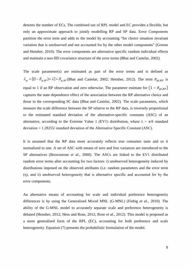
The scale parameter(s) are estimated as part of the error terms and is defined as

RPqtRPqtqt ,, ])1[( ϑλϑλ +×−= (Bhat and Castelar, 2002; Hensher, 2012). The term 𝜗𝑞𝑞,𝑅𝑅 is

equal to 1 if an RP observation and zero otherwise. The parameter estimate for �1 − 𝜗𝑞𝑞,𝑅𝑅�

captures the state dependence effect of the association between the RP alternative choice and

those in the corresponding SC data (Bhat and Castelar, 2002). The scale parameters, which

measure the scale difference between the SP relative to the RP data, is inversely proportional

to the estimated standard deviation of the alternative-specific constants (ASC) of an

alternative, according to the Extreme Value 1 (EV1) distribution, where λ = π/6 standard

deviation = 1.28255/ standard deviation of the Alternative Specific Constant (ASC).

It is assumed that the RP data more accurately reflects true consumer taste and so it

normalized to one. A set of ASC with means of zero and free variances are introduced to the

SP alternatives (Brownstone et al., 2000). The ASCs are linked to the EV1 distributed

random error terms after accounting for two factors: i) unobserved heterogeneity induced by

distributions imposed on the observed attributes (i.e. random parameters and the error term

(η), and ii) unobserved heterogeneity that is alternative specific and accounted for by the

error components.

An alternative means of accounting for scale and individual preference heterogeneity

differences is by using the Generalised Mixed MNL (G-MNL) (Fiebig et al., 2010). The

ability of the G-MNL model to accurately separate scale and preference heterogeneity is

debated (Hensher, 2012; Hess and Rose, 2012; Rose et al., 2012). This model is proposed as

a more generalised form of the RPL (EC), accounting for both preference and scale

heterogeneity. Equation (7) presents the probabilistic formulation of the model.

9

𝑃�𝑗, X𝑞𝑞′ β𝑞𝑞� = 𝑒(x𝑞𝑞,𝑞′ β𝑞𝑞)

∑ 𝑒(x𝑞𝑞,𝑞′ β𝑞𝑞)𝐽𝑞𝑞

𝑞=1

(7)

The parameter estimate 𝜷𝑞𝑞 contains 𝜎𝑞𝑞𝑞𝜷 + 𝜎𝑞𝑞𝑞𝜼𝒒𝒒. The first term includes the parameter

estimate and the simulated individual specific standard deviation of the error term (𝜎𝑞𝑞𝑞). The

second term captures the individual specific unobserved heterogeneity (Γv𝑞𝑞) (Hensher,

2012). The subscript r in the above model signifies the R simulated draws associated with the

optimisation of the simulated log-likelihood function (see Fiebig et al. 2010 for details).

While the subscript s denotes the number of data sources jointly modelled.

While this paper follows the interpretation of the G-MNL as offered by Fiebig et al. (2010),

Greene and Hensher (2010) and Hensher (2012) with regards to the separation of scale and

preference heterogeneity.

In the G-MNL model the scale difference between RP and SC is accounted for via the

individual specific standard error (𝜎𝑖𝑞𝑞) that provides a means of separating data set scale

heterogeneity and individual preference heterogeneity. The individual specific standard error

includes the variance parameter of the scale heterogeneity (τ), the data set specific scale

parameter (𝜛) and control for the number of data sources (ds). So this standard error term

(𝜎𝑞𝑞𝑞) can be expanded:

𝑒[−(𝜏+𝜛𝑑𝑠)2

2 +(𝜏+𝜛𝑑𝑠)𝜔𝑞𝑞] (8)

The wir term in equation (8) is the R simulated draws of unobserved heterogeneity, which is

normally distributed (Hensher, 2012).

3. RP and SC data

Survey responses from a total sample of 1173 individuals are used. The SC data uses 587

respondents who answered Efficient design choice tasks5, while the RP data is from the same

SC respondents and an additional 586 respondents who answered Orthogonal design SC

5See Iles and Rose (2014) for a description and discussion of alternative SC experimental designs and their

impact on literate and illiterate respondents’ behaviour.

10

choice tasks. The unequal number of RP and SC respondents causes the data to be

unbalanced and follows the work of Brownstone, Bunch and Train (2000) in estimating

demand. These authors also use a RPL (EC) model in a combined analysis of revealed and

qualitative data. Combining the RP and SC data, along with the use of exogenous weights, is

akin to having the three sample villages with CHC and PHC facilities, out of the eight

villages sampled, having full availability of the allocated government MBBS provider

facilities. Further details of this assumed availability under the counterfactual scenario is

provided in Appendix B.

Four ‘doctor’ type categories are used in this study. These are: 1) unqualified - jhola chhaap -

providers, 2) private MBBS doctors, 3) government MBBS doctors and 4) Other provider

choice – representing a collection of self-medication, government nurse, traditional forms of

medicine and no treatment. Table I displays the market shares for each provider according to

data type. The RP observations for private MBBS provider are deleted in Table I due to

insufficient data to impute values for the approximate 90 per cent of cases when this provider

type is a non-selected alternative. Further details about imputation of price and distance

values are given below and in Appendix C. The utilisation of government MBBS doctors

under the SC scenario remains surprisingly low at 51 per cent. Other factors effecting

consumer choice to consult government MBBS doctors include: perceived poor quality of

medicines, perceived need to pay informal payments and other factors (Iles, 2014)

Table I: Utilisation of healthcare provider according to survey type Full recall (Unconditional) RP SC* Number percent Number percent Unqualified ‘doctor’ 699 59.6 1815 34.4 Private MBBS doctor - - 702 13.3 Government MBBS doctor 289 24.6 2698 51.1 None (Other) 185 15.8 68 1.3 TOTAL 1173 100.0 5283 100.0 Note: * A central assumption of the SC survey was that government MBBS doctors were always present and available in

and/or surrounding each village.

The descriptive statistics of the full data, including prices, are shown in Table II. The pricing

of outpatient treatment in the selected villages typically includes the cost of medicine and a

consultation fee. This is the case for the majority of unqualified and government doctors in

rural areas who supply their own prescribed medicine. Anecdotally, government centres in

towns (as opposed to villages) may also prescribe medicines not stocked, purposefully or

11

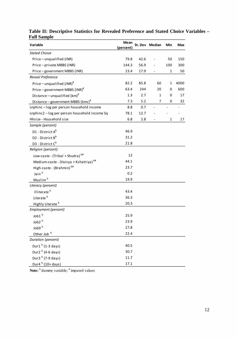
otherwise, forcing consumers to pay for these from private drug stores. The mean and median

RP charges by doctor classification and across the eight villages for first treatment of a

mild—severe fever are: i) unqualified – INR 82.2 and INR 60, and ii) government MBBS –

INR 63.4 and INR 20. Approximately 30 per cent of government consultations were priced at

INR 1.

The price and distance variables of the non-selected healthcare provider alternative are

missing from the original survey. This corresponds to approximately 35 per cent of

unqualified – jhola chhaap – providers and 65 per cent of government MBBS doctors. A

Multivariate Imputation by Chain Equation (MICE) method is used to estimate and fill these

missing values. The R packages MICE and Countimp are used to fill the missing values

following a series of univariate imputations (Kleinke and Reinecke, 2013; van Buuren and

Groothuis-Oudshoorn, 2013). The MICE algorithm, also known as fully conditional

specifications (FCS), employs a Markov Chain Monte Carlo (MCMC) method by using

conditional densities to run the multivariate imputation model for each variable individually

(see Appendix C for more details).

12

Table II: Descriptive Statistics for Revealed Preference and Stated Choice Variables – Full Sample

Variable Mean (percent)

St. Dev Median Min Max

Stated ChoicePrice – unqualified (INR) 79.8 42.6 - 50 150Price – private MBBS (INR) 144.3 56.9 - 100 300Price – government MBBS (INR) 23.4 17.9 - 1 50

Price – unqualified (INR)# 82.2 85.8 60 1 4000

Price – government MBBS (INR)# 63.4 244 20 0 600

Distance – unqualified (km)# 1.3 2.7 1 0 17

Distance – government MBBS (kms)# 7.3 5.2 7 0 32Lnphinc – log per person household income 8.8 0.7 - - -Lnphinc2 – log per person household income Sq 78.1 12.7 - - -Hhsize - Household size 6.8 2.8 - 1 17

D1 - District Ab 46.9

D2 - District Bb 31.2

D3 - District Cb 21.8

Low-caste - (Tribal + Shudra) b# 12

Medium-caste - (Vaisya + Kshatriya) b# 44.1

High-caste - (Brahmin) b# 23.7

Jain b 0.2

Muslim b 19.9

Il l iterate b 43.4

Literate b 36.3

Highly Literate b 20.3

Job1 b 25.9

Job2 b 23.9

Job9 b 27.8

Other Job b 22.4

Dur1 b (1-3 days) 40.5

Dur2 b (4-6 days) 30.7

Dur3 b (7-9 days) 11.7

Dur4 b (10+ days) 17.1

Note: b dummy variable; # imputed values

Reveal Preference

Sample (percent)

Religion (percent)

Duration (percent)

Literacy (percent)

Employment (percent)

13

4. Results

The results presented here are focused on unconditional demand estimates. The RPL model

results are based on the simulated maximisation of the log-likelihood. Two hundred Halton

draws are made from the distributions of the random variables.The Nlogit 5 (Econometric

Software, 2012) software is used for all modelling. The price and income values are all

positive, so distributions allowing only for positive draws are appropriate. Triangular

distributions anchored at zero are used for income random parameters and unqualified – jhola

chhaap - providers, private MBBS and government MBBS prices (Hensher, 2012). As a

result of the mixing of distributions in the residual, interpretations of the coefficients are not

the same as in the base MNL model.

4.1 Unconditional estimates The unconditional demand estimation results presented in Table III are for separate RP and

SC models. The contrasting assumptions regarding the availability of healthcare providers in

the RP and SC data, along with the relative scale, represent important differences between the

data. The assumed full village-based availability and competition among unqualified – jhola

chhaap – providers, private and government MBBS providers in the SC data determines that

the resulting demand estimates are measuring a different consumer market. These results are

hypothetical in the sense that they don’t reflect current market provider availability, but

plausible future markets containing the current market alternatives. The RP data represent

current village-level market realities, with the known uncertainty of government MBBS

provider availability in CHCs and PHCs.

14

Table III: Unconditional Estimates - Revealed Preference and Stated Choice RPL model

Price. -0.001 -0.001 R1: -0.026 R1: -0.021 R1: -0.020

(0.001) (0.001) (0.002) (0.002) (0.003)

-0.074 -0.016 0.037 -1.799 -2.140

(0.028) (0.015) (0.064) (0.091) (0.064)

3.673 3.673 R1: 3.538 R1: 3.538 R1: 3.538

(1.451) (1.451) (0.434) (0.434) (0.434)

-0.249 -0.249 R1: -0.091 R1: -0.091 R1: -0.091

(0.087) (0.087) (0.012) (0.012) (0.012)

0.318 -0.994

(0.049) (0.064)

0.430 0.355 0.417

(0.072) (0.124) (0.088)

-0.213 -0.538 -0.617

(0.094) (0.133) (0.086)

0.454

(0.121)

-0.278

(0.134)

CHCb (base: all other villages) -0.743 0.093

(0.274) (0.363)

PHC1b (base: all other villages) -0.284 -1.004

(0.208) (0.243)

PCH2b (base: all other villages) 0.188 -0.228

(0.287) (0.447)

Job1b (base: all other jobs) 0.287 0.530 0.328 0.647

(0.258) (0.281) (0.396) (0.288)

Job2b (base: all other jobs) 0.555 0.098 1.025 0.818

(0.262) (0.306) (0.438) (0.303)

Job9b (base: all other jobs) 0.454 0.526 0.218 0.021

(0.250) (0.274) (0.415) (0.281)

Low-casteb (base: Brahmin) -0.361

(0.156)

Medium-casteb (base: Brahmin) 0.311

(0.151)

Il l i terateb (base: highlit) 0.570 0.434

(0.191) (0.248)

Li terateb (base: highlit) 0.437 0.623

(0.184) (0.239)Hhs ize -0.056

(0.024)

Dur1b (base: Dur4) -0.308

(0.160)

Dur2b (base: Dur4) -0.717

(0.176)

Dur3b (base: Dur4) -0.353

(0.244)

1.192 0.889

(0.209) (0.173)

0.265 -0.093

(0.279) (0.236)

0.825 0.102 -0.536

(0.303) (0.463) (0.364) - -

13.099 -1.292

- -

- -

Constant

None

-

D3b (base: D1) -

-

- -

- -

-

-

-

-

-

-

-

-

-

-

-

-

-

-

-

-

-

-

-

- - -

- -

- - -

- -

-

-

-

(6.195) (0.149)

-

Recomm x Travel negative a - - -

D2b (base: D1)

-

Recomm. negative a - -

Recomm x Travel pos i tive a - -

-

-

-

-

-

-

Medicine a - - -

Recomm. pos i tive a - -

Travel Dis t. a

Ln Income (per cap).

Ln Income sq (per cap).

Coefficient Coefficient Coefficient

(St. Err.) (St. Err.) (St. Err.) (St. Err.) (St. Err.)

Variables Unqualified Government Unqualified Private GovernmentCoefficient Coefficient

Revealed Preference Stated Choice

15

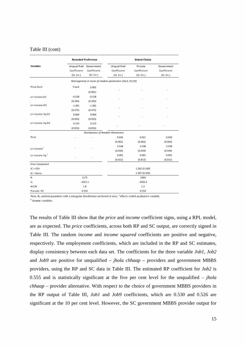
Table III (cont)

The results of Table III show that the price and income coefficient signs, using a RPL model,

are as expected. The price coefficients, across both RP and SC output, are correctly signed in

Table III. The random income and income squared coefficients are positive and negative,

respectively. The employment coefficients, which are included in the RP and SC estimates,

display consistency between each data set. The coefficients for the three variable Job1, Job2

and Job9 are positive for unqualified – jhola chhaap – providers and government MBBS

providers, using the RP and SC data in Table III. The estimated RP coefficient for Job2 is

0.555 and is statistically significant at the five per cent level for the unqualified – jhola

chhaap – provider alternative. With respect to the choice of government MBBS providers in

the RP output of Table III, Job1 and Job9 coefficients, which are 0.530 and 0.526 are

significant at the 10 per cent level. However, the SC government MBBS provider output for

Fixed 0.002

(0.001)

Ln Income:D1 -0.528 -0.528

(0.293) (0.293)

-1.301 -1.301

(0.475) (0.475)

0.064 0.064

(0.033) (0.033)

0.153 0.153

(0.053) (0.053)

- - 0.026 0.021 0.020

(0.002) (0.002) (0.003)

3.538 3.538 3.538

(0.434) (0.434) (0.434)

0.091 0.091 0.091

(0.012) (0.012) (0.012)

JC + None

Note: R1 random parameter with a triangular distribution anchored at zero; a effects coded qualitative variable; b dummy variables.

Pseudo. R2 0.552 0.554

1.292 (0.149)

1.367 (0.102)

N 1173 5283

LL -1022.1 -3265.4

AIC/N 1.8 1.3

Ln Income1 - -

Ln Income Sq.1

- -

Error Component

JC + GDr

Price:Dur2 - - -

- - -

Ln Income:D3 - - -

Ln Income Sq:D1 - - -

Ln Income Sq:D3 - - -

Distributions of Random Parameters

Price

Heterogeneity in mean of random parameters (Dur2, D1,D3)

Variables

Revealed Preference Stated Choice

Unqualified Government Unqualified Private GovernmentCoefficient Coefficient Coefficient Coefficient Coefficient

(St. Err.) (St. Err.) (St. Err.) (St. Err.) (St. Err.)

16

Job1 and Job2 are significant at the five and one per cent levels with coefficient estimates of

0.647 and 0.818.

Covariates for respondents literacy and caste identity are shown to be important determinants

of consumer demand for unqualified – jhola chhaap – providers. Literacy variables are

included in the RP and SC estimates of Table III and are positively signed. Relative to highly

literate respondents, literate respondents are more likely to choose to see an unqualified –

jhola chhaap – provider. The positive coefficients of 0.437 (RP) and 0.623 (SC) are

significant at the five per cent level in both sets of output. Although the illiterate coefficients

are both positive in Table III, their levels of significance differ. In the RP output, the

coefficient of 0.570 is significant at the one per cent level, while in the SC output the

coefficient of 0.434 is significant only at the 10 per cent level. As can also be seen from the

RP output in the table, the dummy variables low-caste and medium-caste, relative to

high-caste (i.e. Brahmin) are statistically significant. In the case of medium-caste, the RP

coefficient of 0.311 is positive and statistically significant at the five per cent level. The

low-caste coefficient of -0.361 is negative and significant at the five per cent level.

The coefficients for recommendation categorical variable are signed appropriately in the

conditional SC output of Table III. The coefficients for positive and negative

recommendations, relative to no recommendation, are highly significant at the one and five

per cent levels. For unqualified – jhola chhaap – providers the positive coefficient is 0.430

and significant at the one per cent level, and the negative is -0.213 and significant at the five

per cent level. Both recommendation coefficients for the qualified MBBS providers are

statistically significant at the one per cent level at the respective values: 0.355 and -0.538 for

private MBBS provider and 0.417 and -0.617 for government MBBS provider. However, the

estimates in Table III show that the interaction between the distance and

recommendationcoefficients, for the private MBBS provider alternative, produce significant

coefficients at the one and five per cent levels. These coefficients at 0.454 and -0.278 are

significant at the one and five per cent levels.

The results on the RP and SC data in Table III include expected endogeneity bias. The

coefficients for price and income in the RP estimates are expected to be biased downwards.

The price and income data from the survey is expected to contain misreporting by

17

respondents. The experimental design used to obtain the SC data prevents this endogeneity

effect. Likewise, the inclusion of fever duration coefficients – Dur1, Dur2 and Dur3 – in the

SC output is expected biased for the same misreporting reason that explained the endogeneity

in RP price and income estimates. The use of fever duration measures as proxies for fever

severity is an important control in demand estimation. The negative coefficients for Dur1,

Dur2 and Dur3, relative to Dur4, indicate that respondents are more likely to consult a

government MBBS provider when suffering from more severe fevers.

Comparative results for the joint estimation of RP and SC data, using RPL and G-MNL

models, are presents in Table IV. Both set of estimates have the SC data are weighted by

0.11111, which is calculated by dividing the implicit weight of 1 by the number of choice (9)

tasks answered by each SC respondents. This use of weights follows the same use by Axsen

et al. (2009). Pooling the two data sets only affects coefficients that are jointly estimated. The

joint estimation of price and income coefficients for unqualified – jhola chhaap – providers

and government MBBS providers helps to correct the expect endogeneity bias of the previous

RP only estimates. All three measures of goodness-of-fit presented in Table IV

(log-likelihood, AIC and BIC) indicate that the RPL (EC) results are better suited to the data.

As a result, results presented in Table IV are discussed with respect to the RPL (EC) only.

The coefficient estimates for the two categorical recommendation variables across the three

providers is revealing of what recommendation information is important to consumers. The

results of Table IV show that the positive recommendation coefficient for unqualified – jhola

chhaap - providers is positively signed and significant at the one per cent level. The

corresponding negative recommendation coefficient is negative, but is not significant at the

10 per cent level. Both the recommendation coefficients for the government MBBS provider

are correctly signed and statistically significant at the one per cent level. The inclusion of

interaction coefficients for distance and positive recommendation for the private MBBS

provider is positively signed and statistically significant at the one per cent level. However,

the inclusion of the interaction terms for private MBBS provider alternative reduces the

significance of the positive recommendation coefficient. The inclusion and statistical

significance of the interaction term Distance x Recommendation for private MBBS providers,

supports the hypothesis that healthcare consumers are willing to by-pass local outpatient

providers to access perceived higher quality, but more distant private providers.

18

Table IV: Unconditional Estimates - Joint Revealed Preference and Stated Choice

Coefficent (St.error) Coefficent (St.error)UnqualifiedPrice RP.SC R1: -0.019 (0.003) R1: -0.025 (0.002)

Ln Income (household pp)RP.SC R1: 0.497 (0.115) R1: -0.332 (0.119)Ln Income Sq. (household pp) RP R1: -0.241 (0.064) R1: -0.351 (0.102)

Ln Income Sq. (household pp) SC R1: -0.217 (0.036) R1: -0.231 (0.029)Dist.At Home (base:in village)SC 0.150 (0.062) 0.110 (0.059)Distance RP -0.062 (0.044) -0.062 (0.042)Med.Pill & Inject. (base: Pill) SC 0.290 (0.054) 0.296 (0.052)Recom. + ve (base: none) SC 0.387 (0.073) 0.336 (0.067)Recom. – ve (base: none) SC -0.024 (0.099) -0.053 (0.087)CHCb (base: all other villages)RP.SC -0.815 (0.257) -0.474 (0.204)PHC1b (base: all other villages)RP.SC -0.678 (0.188) -0.707 (0.136)PCH2b (base: all other villages)RP.SC -0.221 (0.300) -0.315 (0.250)Job1b (base: all other jobs)RP.SC 0.371 (0.239) 0.582 (0.271)Job2b (base: all other jobs)RP.SC 0.752 (0.259) 1.030 (0.278)Job9b (base: all other jobs)RP.SC 0.099 (0.237) 0.159 (0.258)Low-casteb (base: Brahmin)RP -0.574 (0.237) -0.619 (0.225)Medium-casteb (base: Brahmin)RP 0.421 (0.220) 0.438 (0.207)Illiterateb (base: highlit)RP.SC 0.757 (0.188) 0.633 (0.135)Literateb (base: highlit)RP.SC 0.679 (0.177) 0.661 (0.131)ConstantRP 2.386 (0.283)Government MBBSPrice RP.SC R1: 0.037 (0.002) R1: -0.031 (0.020)

Ln Income (household pp)RP.SC R1: 0.497 (0.115) R1: -0.332 (0.119)Ln Income Sq. (household pp) RP R1: -0.241 (0.064) R1: -0.351 (0.102)

Ln Income Sq. (household pp) SC R1: -0.217 (0.036) R1: -0.231 (0.029)Dist.5-15 kms (base: in village) SC -2.245 (0.067) -1.919 (0.057)Distance RP -0.021 (0.021) -0.031 (0.020)Med.Medicine cost (base: free) SC -1.061 (0.070) -0.945 (0.065)Recom. + ve (base: none) SC 0.711 (0.093) 0.536 (0.085)Recom. – ve (base: none) SC -0.668 (0.094) -0.509 (0.085)Dist. x Recomm. (+ve) SC 0.134 (0.084) 0.151 (0.077)Dist. x Recomm. (-ve) SC 0.087 (0.100) -0.023 (0.096)Job1b (base: all other jobs)RP.SC 0.815 (0.295) 0.831 (0.259)Job2b (base: all other jobs)RP.SC 0.341 (0.278) 0.780 (0.250)Job9b (base: all other jobs)RP.SC 0.228 (0.267) 0.198 (0.226)Dur1b (base: Dur4) SC -0.233 (0.227) -0.289 (0.110)Dur2b (base: Dur4) SC -0.653 (0.242) -0.588 (0.117)Dur3b (base: Dur4) SC -0.118 (0.345) -0.287 (0.169)District 2 (base: sample1) SC 0.389 (0.229) 0.389 (0.229)District 3 (base: sample1) SC -0.051 (0.303) -0.051 (0.303)ConstantRP -2.503 (0.337) -2.503 (0.337)Private MBBSPrice SP R1: -0.013 (0.003) R1: -0.011 (0.003)

Ln Income (household pp) SC R1: 0.497 (0.115) R1: -0.332 (0.119)Ln Income Sq. (household pp) SC R1: -0.217 (0.036) R1: -0.231 (0.029)Dist.5-15 kms (base: in village) SC -1.701 (0.092) -1.661 (0.091)Recom. + ve (base: none) SC 0.033 (0.128) -0.011 (0.121)Recom. – ve (base: none) SC -0.397 (0.142) -0.470 (0.139)Dist. x Recomm. (+ve) SC 0.440 (0.125) 0.355 (0.125)Dist. x Recomm. (-ve) SC -0.340 (0.141) -0.350 (0.141)NoneConstant RP.SC 8.250 (7.537) 22.963 (7.988)

JC (RP, SC) R2: 0.535 (0.162)Gdr (RP, SC) R2: 1.201 (0.125)None (RP, SC) R2: 0.448 (0.329)Tau 0.121 (0.038)

State Dependence R1: 1.805 (0.378) R1: -3.115 (0.335)

RPL (EC) weighted

Generalised Mixed MNL weighted

Model A Model B

State Dependence

Scale Parameters

19

Table IV (cont)

The preferences of north Indian healthcare consumers in different employment categories

appear to differ, when controlling for Hindu caste identity, income, literacy, severity of fever

and proximity of local government PHCs and CHC. The coefficient for Job2 remains positive

and highly statistically significant when choosing to consult an unqualified – jhola chhaap –

provider. However, there is no apparent statistical significance for Job2 or Job3 for

government MBBS provider choice. Only Job1 is positively signed and statistically

significant at the 10 per cent level.

Both the dummy variable coefficients for illiterate and literate are positive and significant at

the one per cent level for unqualified – jhola chhaap – providers. The positive sign of these

coefficients, relative to highly literate consumers (i.e. those with senior secondary and above

levels of education), suggests that highly literate respondents are less likely to consult

unqualified village based providers.

Two distance coefficients are presented in Table IV – related separately to the RP and SC

data. The different measurement method underpinning each variable prevents their joint

Coefficent (St.error) Coefficent (St.error)

Price-JC <0.001 (<0.001) 0.001 (<0.001)

Price-GDr -0.001 (0.001) -0.001 (<0.001)

Price-PDr -0.005 (0.001) -0.005 (0.002)

Ln Income 1.117 (0.380) 1.661 (0.392)Ln Income Sq. RP -0.066 (0.026) -0.103 (0.029)Ln Income Sq. SC -0.043 (0.022) -0.095 (0.026)

Price-JC 0.019 (0.003) 0.024 (0.002)Price-GDr 0.037 (0.007) 0.011 (0.003)Price-PDr 0.013 (0.003) 0.017 (0.002)Ln Income 0.497 (0.115) 0.332 (0.119)Ln Income Sq.RP 0.241 (0.064) 0.231 (0.029)Ln Income Sq.SC 0.217 (0.036) 0.351 (0.102)State Dependence 1.805 (0.378) 3.115 (0.335)

JC(SC) + JC(RP) 0.429 (0.171)GDr (SC) + GDr(RP) 1.035 (0.127)Heterogeneity in GMXL scale factor (SC) -0.371 (0.026)LL -4313.9 -4460.2AIC 8749.8 9034.5BIC 9162.9 9420.5R1 random parameter with triangular dis tribution; R2 random parameter with a normal dis tribution;

SC Stated Choice data; RP Revealed Preference data; b imputed miss ing va lues .

Distribution of Random Parameters

Error Components

RPL (EC) weighted

Generalised Mixed MNL weighted

Model A Model B

Heterogeneity in Mean (income)

20

estimation. The distance coefficients for both qualified MBBS providers are negative. In the

case of the government MBBS provider the continuous variable is statistically significant at

the one per cent level.

The outpatient fever treatment demand estimates for rural UP show that consumers value the

recommendation of respected family members or friends for healthcare providers in different

ways. Positive recommendations have a positive effect in determining whether to consult

unqualified – jhola chhaap – providers to treat a mild-severe fever. The lack of

corresponding importance in negative recommendations for the same providers suggests that

healthcare consumers are less critical of the quality of unqualified providers who generally

operate in the immediate village context. However, the dual importance of positive and

negative recommendations, for government MBBS providers, suggests consumers weigh

both positive and negative recommendations when making their choice of whether to consult

a government MBBS provider.

The importance of consumer occupation in determining demand for unqualified – jhola

chhaap – providers is supported by unconditional demand estimates. Those in a labouring

occupation have an increased likelihood of demanding the health services for a mild-severe

fever from unqualified – jhola chhaap – providers. The importance of labouring occupation,

while controlling for other social capital measures – caste identity and literacy, supports the

hypothesis that occupations are an important social network affecting healthcare

decision-making.

5. Simulated demand elasticities

The own-price demand elasticities for unqualified – jhola chhaap – providers and

government MBBS providers are calculated using the unconditional RP and joint RP and SC

demand estimations from Tables III and IV6. The two sets of estimates provide estimates for

6The simulated elasticities are derived using the original estimated choice probabilities from the RPL (EC)

models and are reallocated in the simulation according to the specifications. In keeping with the non-IID error

distributions, the choice probabilities are not made proportionally in the simulation of the price elasticities. The

arc-price elasticities are calculated using a probability weighting. Therefore, a probability weighted sample

enumeration (PWSE) technique is used. The formula for the PWSE is given below:

21

i) the current level of healthcare provider competition in rural UP and ii) counterfactual

market demand.

The RP own-price demand elasticities in Table V are relative inelastic. At the lowest price

interval for government MBBS providers (INR 1-25) the estimates range between -0.01 to

-0.02 across the four income quartiles (QR1to QR4). The elasticities increase within each

income quartile as prices increase. At the interval INR 126-150 the range of elasticities range

between -0.03 to -0.04. The own-price elasticities for unqualified – jhola chhaap – providers

are larger. Within Table V the estimates at the lowest price interval (INR1-50) are -0.03 to

-0.04. This increases to a range of -0.10 to -0.11 at the interval INR 251-300. For both

providers, little or no change is evident across income quartiles.

Table V: Unconditional RP own-price elasticities for unqualified – jhola chhaap – providers and government MBBS providers

The RP own-price demand elasticity estimates of Table V are higher for unqualified – jhola

chhaap – providers than for government MBBS providers. The own-price demand elasticities

are expected to by higher due to the combined reasons of i) greater level of village-based

competition among jhola chhaap fever services, and ii) generally perceived lower levels of

where 𝑃�𝑞 refers to the aggregate probability of the choice of alternative j, 𝑃�𝑞𝑞 is an estimated choice probability

and ..jq

jkq

jkq

jqPX P

XXP

E jq

jkq ∂∂

= In turn 𝑋�𝑞𝑞𝑞is the mean price between two points and 𝑃�𝑞𝑞 is the corresponding mean

probability for individual q, alternative j and individual attribute k.

Va: Own-price RP JC

Price interval (INR) QR1 QR2 QR3 QR4

1-50 -0.04 -0.04 -0.03 -0.03101-150 -0.06 -0.07 -0.07 -0.07251-300 -0.11 -0.10 -0.10 -0.10

Vb: Own-price RP GdrPrice interval (INR) QR1 QR2 QR3 QR4

1-25 -0.01 -0.02 -0.01 -0.0151-75 -0.02 -0.03 -0.02 -0.02

126-150 -0.03 -0.04 -0.03 -0.03

22

clinical quality among these providers. More competition should drive down prices and make

consumers more price sensitive to price increases. Relative to government MBBS services,

the clinical quality of unqualified – jhola chhaap– providers is generally considered lower.

Thus, systematic price increases among jhola chhaaps would see some consumers demand

more Other fever treatment services from within the village.

The unqualified – jhola chhaap– provider hypothetical estimates are presented in Table VIa.

At all levels the elasticities are greater than those estimated for the RP only data. The Table

shows that as prices increase the degree of own-price elasticity increases within each income

quartile. In the first income quartile (QR1) the elasticities increase from -0.21 at the price

interval INR 1-50 to -0.74 at the price interval INR 251-300. The corresponding elasticities

for the fourth quartile (QR4) range from -0.14 to -0.62. The own-price elasticities decrease as

incomes increase within each price interval. For the interval INR 51-100 the elasticities

decrease from -0.31 in QR1 to -0.23 in QR4. This pattern is consistent across all price

intervals. The combined characteristics of increasing price elasticities as prices increase and

decreasing elasticities as increase rise is consistent with microeconomic theory. These higher

unqualified – jhola chhaap – provider estimates, under the hypothetical scenario of greater

certainty of availability of government MBBS providers, reflects consumers’ greater price

sensitivity due to a more reliable supply of lower single-visit cost government providers.

23

Table VI: Unconditional pooled and weighted own-price elasticities for unqualified – jholachhaap– providers (VIa) and government MBBS providers (VIb)

The corresponding own-price demand elasticities for government MBBS provider are

presented in Table VIb. For government MBBS providers the elasticity estimates are also

higher at each price interval, compared to the RP estimates. Within an income quartile the

elasticities rise. In QR1 the own-price elasticities rise from -0.04 for the INR 1-25 interval to

-0.06 for the INR 126-150 interval. Within each income quartile the pattern of increasing

own-price elasticity is consistent. The results from Table 6b show that own-price elasticities

increase, for a given price interval, as incomes rise. At the lowest price interval INR 1-25 the

elasticities are -0.04 (QR1), -0.07 (QR2), -0.11 (QR3) and -0.14 (QR4). Likewise, at the

highest price interval INR 126-150 the own-price elasticities progressively increase: -0.06 in

QR1, -0.12 in QR2, -0.17 in QR3 and -0.27 in QR4. The increasing own-price elasticities

among higher income groups reflects the possible greater awareness and expectation of free

healthcare at government healthcare facilities among those with higher incomes, whilst

having to make informal payments. The importance of this factor in explaining the rising

own-price elasticity is justified as the importance of the other perceived reasons for non-

utilisation of government services ‘Too far to travel’ would be lessened under the

counterfactual assumption. The other perceived reason ‘Poor quality medicine’ has an

uncertain expected relationship with household income.

Price-interval (INR) QR1 QR2 QR3 QR4

1-50 -0.21 -0.18 -0.16 -0.1451-100 -0.31 -0.27 -0.25 -0.23

101-150 -0.43 -0.39 -0.37 -0.34151-200 -0.53 -0.48 -0.46 -0.44201-250 -0.67 -0.61 -0.58 -0.55251-300 -0.74 -0.68 -0.65 -0.62

Price-interval (INR) QR1 QR2 QR3 QR4

1-25 -0.04 -0.07 -0.11 -0.1426-50 -0.05 -0.09 -0.13 -0.1851-75 -0.06 -0.11 -0.16 -0.2376-100 -0.05 -0.11 -0.16 -0.24

101-125 -0.06 -0.12 -0.17 -0.26126-150 -0.06 -0.12 -0.17 -0.27

Note: JCrp and Gdrrp refer to arc-elastici ties only us ing the RP variable estimates of the

jointly model led SC and RP data .

VIa: Own-price JCrp

VIb: Own-price Gdrrp

24

Cross-price elasticities are presented in Table VIIa and b. These results show that under the

scenario of greater government doctor availability the cross-price elasticity for government

MBBS doctor, given demand for unqualified – jhola chhaap – providers, services is

relatively high compared to Other options. In the first income quartile (QR1), presented in

Table VIIa, the cross-price elasticity for government providers ranges between 0.48 at the

price interval INR 1-50 to 0.51 for the price interval INR 201-250. The corresponding cross-

price elasticity for the Other category is 0.16 at the price interval INR 1-50 and 0.22 for the

interval INR 201-250. Among higher incomes in QR4 the government elasticity is 0.53 and

0.65 and for the Other category it is 0.09 and 0.15. The opposing cross-price elasticities,

given demand for government MMBS doctor services presented in Table VIIb, are much

lower ranging between 0.02 to 0.06 for unqualified – jhola chhaap – providers and <0.01 to

0.02 for Other providers. The cross-price elasticity results indicate that consumer are more

price sensitive to increase in the price of unqualified – jhola chhaap – providers. Consumer

are more willing to move to access government MBBS services, under the assumed greater

availability for government providers, for price increases in competing services. This greater

price sensitivity may indicate that north Indian consumers implicitly make price-quality

trade-offs and that they are less willing to pay more (fees and access costs) for lower quality

unqualified – jhola chhaap – provider services.

Table VII: Unconditional pooled and weighted cross-price elasticities given demand for unqualified – jhola chhaap – providers (VIIa) and government MBBS providers (VIIb)

Increasing the availability of government MBBS providers in rural UP is expected to make

healthcare consumers more price sensitive. This increase in own-price elasticity is true for

Price-interval (INR) Gdrrp Other Gdrrp Other Gdrrp Other Gdrrp Other1-50 0.48 0.16 0.51 0.14 0.49 0.12 0.53 0.09

101-150 0.50 0.20 0.58 0.19 0.60 0.17 0.63 0.13201-250 0.51 0.22 0.55 0.20 0.60 0.19 0.65 0.15

VIIb: Cross-price: JCrp, Other (given demand for Gdrrp)

Price-interval (INR) JCrp Other JCrp Other JCrp Other JCrp Other1-25 0.02 0.01 0.03 0.01 0.04 0.01 0.05 0.0151-75 0.03 0.01 0.04 0.02 0.05 0.01 0.06 0.01

101-125 0.03 <0.01 0.04 0.02 0.05 0.01 0.06 0.01Note: JCrp and Gdrrp refer to arc-elastici ties only us ing the RP variable estimates of the jointly model led SC and RP data .

VIIa: Cross-price: Gdrrp, Other (given demand for JCrp)QR1 QR2 QR3 QR4

QR1 QR2 QR3 QR4

25

government MBBS and unqualified – jhola chhaap – provider fever treatment services. This

increase in price elasticity of demand is predicted by microeconomic theory due the close

substitutes of government MBBS and unqualified – jhola chhaap – provider fever treatment

services.

6. Concluding Comments

The value of jointly modelling RP and SC data in this work is that it offers market-based

predictions of demand while allowing for increased trade-offs under the counterfactual

scenario. The assumed complete availability of government MBBS providers in the SC data,

combined with the RP data, provided market scenarios akin to a situation where all current

CHCs and PHCs have consistent availability of allocated government MBBS providers. This

method of counterfactual estimation does not assume that consumers’ trade-offs across

attributes are fixed between the two scenarios. As a result, the approach allows for more

behavioural accuracy in estimating consumer demand under the counterfactual scenario.

Demand estimates presented here indicate that uncertainty of government MBBS provider

availability is a barrier to increasing the market share of government health centres in treating

outpatient fever patients. The large market share of jhola chhaaps providers is despite the

higher initial prices of these providers. Results from the SC data reveals that removal of the

availability barrier associated with government MBBS providers increases their respective

market share. In this scenario, the expected marginal benefit of better health offered by

government MBBS providers outweighs the combined expected marginal cost of paying

informal fees and travel costs.

The hypothesis that consumers perceive the quality of care of unqualified – jhola chhaap –

providers is generally lower than that provided by government MBBS doctors is affirmed.

The findings that consumers’ predominantly use positive recommendations in choosing to

access fever treatment from unqualified – jhola chhaap – providers, while using both positive

and negative recommendations when choosing to seek fever treatment from government

MBBS providers, attests to an expected lower quality of care offered by jhola chhaap. The

relatively higher cross-price elasticity of jhola chhaaps, given the counterfactual demand for

government MBBS, also supports this hypothesis.

26

The demand elasticity estimates presented in this work suffer from uncontrolled endogeneity

associated with fever duration and income parameters and the relatively large amount of

imputation conducted for non-selected government MBBS provider alternatives’ price and

distance data among the RP data. Both endogenous variables are expected to suffer from

measurement error in a non-random way.

In the context of current debate surrounding India’s commitment towards delivering universal

healthcare, demand predictions assuming greater certainty of government MBBS provider

availability is insightful. The removal of government doctor absenteeism in rural north India

is not sufficient to ensure that consumer demand for outpatient fever treatment is satisfied

within the public system. The role of unqualified – jhola chhaap – providers would remain

vital. Ways of incorporating these informal providers into any universal health scheme

appears a justifiable avenue for further consideration and research.

27

References Ahmed SM, Hossain MS, Kabir M., 2014. Conventional or Interpersonal Communication: Which Works Best in Disseminating Malaria Information in an Endemic Rural Bangladeshi Community? PloSOne 9, 3.

Banerjee A, Deaton A, Duflo E., 2004. Wealth, health, and health services in rural Rajasthan. The American Economic Review 94, 326-330.

Banerji A, Jain S., 2007. Quality dualism. Journal of Development Economics 84, 234-250.

Basak SC, Sathyanarayana D., 2012. Exploring knowledge and perceptions of generic medicines among drug retailers and community pharmacists. Indian Journal of Pharmaceutical Sciences 74, 571-575.

Ben-Akiva M, Lerman S., 1985. Discrete Choice Analysis: Theory and Application to Transport Demands. The MIT Press: Cambridge, Massachusetts.

Ben-Akiva M, Morikawa T., 1990. Estimation of switching models from revealed preferences and stated intentions. Transportation Research Part A: General 24, 485-495.

Bhat CR, Castelar S., 2002. A unified mixed logit framework for modeling revealed and stated preferences: formulation and application to congestion pricing analysis in the San Francisco Bay area. Transportation Research Part B: Methodological 36, 593-616.

Böhme M, Thiele R., 2011. Is the informal sector constrained from the demand side? Evidence for six west African capitals. World Development 40, 1369-1381.

Borah BJ., 2006. A mixed logit model of health care provider choice: analysis of NSS data for rural India. Health Economics 15, 915-932.

Brand JPL., 1999. Development, Implementation and Evaluation of Multiple Imputation Strategies for the Statistical Analysis of Incomplete Data Sets. Doctor of Philosophy. Erasmus University: Rotterdam.

28

Brownstone D, Bunch DS, Train K., 2000. Joint mixed logit models of stated and revealed preferences for alternative-fuel vehicles. Transportation Research Part B: Methodological 34, 315-338.

Chang FR., Trivedi PK., 2003. Economics of self-medication: theory and evidence. Health Economics 12, 721-739.

Chaudhury N, Hammer J, Kremer M, Muralidharan K, and Rogers FH., 2006. Missing in action: teacher and health worker absence in developing countries. The Journal of Economic Perspectives, 20, 91-116.

Cherchi E, Ortúzar JDD., 2011. On the use of mixed RP/SP models in prediction: Accounting for systematic and random taste heterogeneity.Transportation Science 45, 98-108.

Cowles MK, Carlin BP., 1996. Markov Chain Monte Carlo convergence diagnostics: a comparative review. Journal of the American Statistical Association 91, 883-904.

Das J., Das S., 2003. Trust, learning and vaccination: a case study of a north Indian village. Social Science and Medicine 57, 97-112.

Das J., Hammer J., 2007. Money for nothing: The dire straits of medical practice in Delhi, India. Journal of Development Economics 83, 1-36.

Das J, Holla A, Das V, Mohanan M, Tabak D, Chan B., 2012. In urban and rural India, a standardized patient study showed low levels of provider training and hugh quality gaps. Health Affairs 31, 2774-2784.

Dow WH., 1995. Unconditional demand for curative health inputs: does selection on health status matter in the long run? Labor and Population Program Working Paper Series. RAND: Santa Monic, CA.

29

Dussault G., Franceschini MC., 2006. Not enough there, too many here: understanding geographical imbalances in the distribution of the health workforce. Human Resources for Health4 (12).

El Adlouni S, Favre A-C, Bobée B., 2006. Comparison of methodologies to assess the convergence of Markov Chain Monte Carlo methods. Computational Statistics and Data Analysis 50, 2685-2701.

Ensor T., 2004. Informal payments for health care in transition economies. Social Science and Medicine 58, 237-246.

Erlyana E, Damrongplasit KK, Melnick G., 2011. Expanding health insurance to increase health care utilization: will it have different effects in rural vs urban areas? Health Policy 100, 273-281.

Fiebig DG, Keane MP, Louviere J, Wasi N., 2010. The generalized multinomial logit model: accounting for scale and coefficient heterogeneity. Marketing Science 29, 393-421.

Gertler P, Locay L, Sanderson W., 1987. Are user fees regressive - the welfare implications of health-care financing proposals in Peru. Journal of Econometrics 36, 67-88.

Greene WH, Hensher DA., 2010. Does scale heterogeneity across individuals matter? An empirical assessment of alternative logit models. Transportation 37, 413-428.

Grossman M., 1972. The demand for health: a theoretical and empirical investigation. National Bureau of Economic Research, Occasional Paper 119; Columbia University Press: New York.

Hensher DA., 2012. Accounting for scale heterogeneity within and between pooled data sources. Transportation Research Part A: Policy and Practice 46, 480-486.

Hensher DA, Rose JM, Greene WH., 2008. Combining RP and SP data: biases in using the nested logit `trick' - contrasts with flexible mixed logit incorporating panel and scale effects. Journal of Transport Geography 16, 126-133.

30

Hess S, Rose JM., 2012. Can scale and coefficient heterogeneity be separated in random coefficient models? Transportation 39, 1225-1239.

Holte, JH, Kjaer T, Abelsen B, Olsen JA., 2015. The impact of pecuniary and non-pecuniary incentives for attracting young doctors to rural general practice. Social Science & Medicine128, 1-9.

Iles, RA., 2014. Demand for qualified and unqualified primary healthcare in rural north India. Ph.D Thesis. Griffith University, Brisbane.

Iles RA, Rose JM., 2014. Stated Choice design comparison in a developing country: recall and attribute nonattendance. Health Economics Review4, 25.

Kleinke K, Reinecke J., 2013. countimp 1.0 - A Multiple Imputation Package for Incomplete Count Data.http://www.uni-bielefeld.de/soz/kds/pdf/countimp.pdf (accessed: 12.12.14).

Leonard KL, Adelman SW, Essam T., 2009. Idle chatter or learning? Evidence of social learning about clinicians and the health system from rural Tanzania. Social Science & Medicine 69, 183-90.

Mæstad O., Mwisongo A., 2011. Informal payments and the quality of health care: Mechanisms revealed by Tanzanian health workers. Health Policy 99, 107-115.

McCloskey, D., 1987. Counterfacuals. In The New Palgrave: A Dictionary of Economics. Eds J Eatwell, M Milgate and P Newman. Vol 1, 701-703.

Mebratie A.D., Sparrow R., Yilma Z., Alemu G., Bedi A.S., 2015. Enrollment in Ethiopia’s Community-Based Health Insurance Scheme. World Development 74, 58-76.

Meenakshi JV, Banerji A, Manyong V, Tomlins K, Mittal N, Hamukwala P., 2012. Using a discrete choice experiment to elicit the demand for a nutritious food: willingness-to-pay for orange maize in rural Zambia. Journal of Health Economics 31, 62-71.

31

National Sample Survey Organisation, 2015. Key Indicators of Social Consumption in India Health, NSS 71st round (January to June, 2014).

Ozawa S., Walker DG., 2011. Comparison of trust in public vs private health care providers in rural Cambodia. Health Policy and Planning 26, i20-i29.

Pinto S., 2004. Development without Institutions: Ersatz Medicine and the Politics of Everyday Life in Rural North India. Cultural Anthropology 19, 337-364.

Qian D, Pong RW, Yin A, Nagarajan KV, Meng Q., 2009. Determinants of health care demand in poor, rural China: the case of Gansu province. Health Policy and Planning 24, 324-334.

Rose JM, Hess S, Greene WH, Hensher DA., 2012. The generalised multinomial logit model: misinterpreting scale and preference heterogeneity in discrete choice models or untangling the un-tanglable? 13th International Conference on Travel Behaviour Research. Toronto, Canada.

Stuckler D, Feigl AB, Basu S, McKee M., 2010. The political economy of universal healthcare coverage, inFirst Global Symposium on Health Systems Research. Montreux, Switzerland.

The World Bank. 1998. Uttar Pradesh and Bihar Living Conditions Survey data. http://econ.worldbank.org/WBSITE/EXTERNAL/EXTDEC/EXTRESEARCH/EXTLSMS/0,,contentMDK:21387345~pagePK:64168445~piPK:64168309~theSitePK:3358997,00.html. (Accessed: 3 September 2014).

van Buuren S., 2012. Flexible Imputation of Missing Datas. Chapman and Hall/CRC: Boca Raton.

van Buuren S, Boshuizen HC, Knook DL., 1999. Multiple imputation of missing blood pressure covariates in survival analysis. Statistics in Medicine 18, 681-694.

32

van Buuren S, Groothuis-Oudshoorn K., 2011. mice: Multivate Imputation by Chain Equations in R.Journal of Statistical Software 45, 1-67.

Vujicic M., Alfano M., and Shengelia B., 2010. Getting health workers to rural areas: innovative analytic work to inform policy making. Health, Nutrition and Population Discussion Paper. The World Bank. New York.

Willis JR, Kumar V, Mohanty S, Kumar A, Singh JV, Ahuja RC, et al., 2011. Utilization and perceptions of neonatal healthcare providers in rural Uttar Pradesh, India. International Journal for Quality in Health Care: Journal of the International Society for Quality in Health Care. 23, 487-94.

33

Appendix A

Table A1 provides data on perceived reasons for non-government MBBS doctor service

utilisation. The seven reasons for non-use are i) government doctor not in village, ii)

government doctor not available in village, iii) need to pay for medicines, iv) need to pay for

consultation, v) poor quality of government medicines, vi) too far to travel, and vii) other

reason. On average,63.7 per cent of respondents nominated that they did not utilise

government MBBS provider services. The two most cited reasons were i) government MBBS

doctor not in village at 19.3 per cent, and ii) government MBBS doctor not available in

village at 13.1 per cent. These two respondent fields measure in differing ways the

widespread problem of government doctor absenteeism within the sample.

Villages One and Eight, which had a government Community Health Centre (CHC) and

Primary Health Centre (PHC), both recorded zero per cent for this first category. In Village

One, 25.3 per cent of respondents indicated that the unavailability of government doctors was

the primary reason for their non-use of government MBBS outpatient services. In Village

Eight the percentage was 18.0 per cent in the same category of non-availability. However,

Village Two, which also had a PHC, had 18.5 per cent of respondents nominate ‘government

doctor not in village’ and 21.2 per cent nominate ‘government doctor not available’ as the

primary reasons for not utilising government MBBS outpatient services. Key-informant

interviews with the elected village leader from Village Two indicated that the PHC was

generally closed. Across three visits to this village the PHC was closed on each occasion.

This continual closure of the PHC in Village Two helps explain the high percentage of

respondents who recorded ‘government doctor not in village’, despite having a government

PHC located there.

34

Table A1: Reasons for non-use of government doctors by village (% of all respondents). Reasons Village

One^ Village

Two* Village Three

Village Four

Village Five

Village Six

Village Seven

Village Eight*

Gov't Dr not in village 0.2 18.5 26.7 22.9 26.8 27.7 18.0 0.0 Gov't Dr not available in village 25.3 21.2 24.1 15.7 6.8 0.0 1.5 18.1 Pay for medicines 0.0 0.2 1.6 1.1 1.2 1.0 17.2 15.1 Pay for consultation 0.2 2.9 0.0 0.0 0.0 0.1 8.0 14.3 Poor quality medicines 20.5 10.4 3.5 1.2 8.1 1.3 6.7 25.9 Too far to travel 0.0 5.3 10.6 17.3 6.7 8.9 18.6 0.0 Other 12.0 11.4 11.9 9.9 1.2 0.0 12.1 3.0 sub-total 58.2 69.9 78.5 68.1 50.7 38.9 82.0 76.4 N 77 190 110 174 168 197 123 135 Note: ^ denotes the presence of a Community Health Centre (CHC); * denotes the presence of a Primary Health Centre (PHC).

35

Appendix B

Combining the RP and SC data creates a new village-level hypothetical market. If

village-level government MBBS provider availability is measured using an index, the SC

data assumes full availability in half the villages. The two distance attribute levels i) in

village and ii) 5-15 km away averages out to equate to half of the villages having a

government MBBS provider. By contrast, the RP accounts only for the three sample villages

with government MBBS providers. The actual availability of these government providers is

not known. However, over repeated visits to the three government health centres the MBBS

providers were not present. In calculating the availability index it is assumed that at these

three government health centres MBBS providers are available 33 per cent of the time. This

equates to an availability score of 0.124 (i.e. 3/8*0.33).

Pooling the RP and SC data, with and without the weights, provides intermediate availability

scores. These intermediate scores are calculated by multiplying the above SC and RP base

availability score by the proportion of each data type, weighted accordingly. The availability

score formulas for pooled data are:

Availability score pooled = (observationSC/total observationRP+SC) x baseavailability SC+

(observationRP/total observationRP+SC) x baseavailability RP, and

Availability score weighted pooled = ((observationSC/9)/(total observationRP+SC/9) x baseavailability

SC+

(observationRP/total observationRP+SC/9) x baseavailability RP

The pooled availability score is 0.432 = (0.8183 x 0.5)SC + (0.1817 x 0.124)RP. The

proportion of SC and RP observations, within the dataset is 0.8183 = 5283 / 6456 and 0.1817

= 1173 / 6456. By contrast, the weighted pooled availability score is 0.249 = (0.3335 x 0.5)SC

+ (0.6665 x 0.124)RP. The proportion of the data from each data type changes in the weighted

pooled calculation. The SC number of observations is divided by nine to scale the number of

SC observation per respondent to equal 1. As a result, the proportion of SC data is 0.3335 =

(5283/9) / (5283/9 + 1173), and the proportion of RP data is 0.6665 = 1173 / (5283/9 + 1173).

36

The range of government MBBS provider availability are estimated at the levels 0.124 (RP

only), 0.249 (RPSC pooled and weighted), 0.432 (RPSC pooled) and 0.5 (SC only). The

socially optimal availability score in the short run, where all government MBBS providers are

fully available in the three village government health centres, is 0.375 = 3/8. This optimal

short-run score is between the RPSC pooled and the RPSC pooled and weighted.

37

Appendix C

Due to the sequential nature of the MICE algorithm each variable with missing data may use

a different distribution from which to draw imputations.

A Bayesian procedure is used to update the prior distributions from the preceding posteriors.

This iterative approach is completed over a given number of cycles. The number of iterations

used in this study ranged between five and seven. This number is sufficient due to low levels

of autocorrelation among regression variables and the limited amount of memory occupied in

MICE algorithm while running the imputation model (van Buuren, 2012). The work of Brand

(1999) and van Buuren et al. (1999) use between five and twenty iterations.

Evaluating the convergence of the MCMC process is necessary to ensure that a stationary

distribution is reached. Reviews of convergence testing methods find that machine generated

tests are unreliable (Cowles and Carlin, 1996; El Adlouni et al., 2006). Cowles and Carlin

(1996) conclude that machine generated tests should be avoided. As such, visual inspection

of the plots of the mean and standard deviations of the individual imputed variables at each

iteration is used to check that free movement across the iterations occurs.

The missing data imputed as part of this chapter includes the price and categorical distances

for the alternative (non-selected) doctors for respondents and the caste affiliation of

respondents in District A. The assumption of Missing At Random (MAR) appears relevant to

the case of the missing caste data from all respondents in District A. Within the sub-sample

of District A respondents, all caste data has an equal probability (p = 1) of being missing (van

Buuren, 2012). In this case, knowledge of the mechanism of missingness makes the

assumption of MAR clear.

The MAR assumption for the missing data associated with the non-selected alternatives also

holds. Within each healthcare provider alternative, the probability of the data being

non-selected has an equal probability. This second set of missing data is associated with

whether consumers sought treatment from multiple providers. The association between

whether the initial provider was an unqualified – jhola chhaap – provider or a government

MBBS provider is not a determining factor in whether additional providers were sought. As a

result, this data may also be considered MAR.

38

Price

Figure C1:Frequency distribution of unqualified - jhola chhaap–price, original responses and combined original and imputed

Figure C2:Frequency distribution of government MBBS doctor price, original responses and combined original and imputed prices

39

The price of INR 5000 for a single consultation to a government doctor, depicted in Figure

8.3, is an outlier. This value is dramatically greater than all other values. As such, this

observation was deleted reducing the number of observations from 1174 to 1173.

Figure C3: Distribution of government MBBS doctor prices, original and combined original and imputed prices

Distance

Figure C4:Frequency distribution of distance to unqualified - jhola chhaap - provider original responses and combined original and imputed prices

40

Figure C5:Frequency distribution of distance to government MBBS doctor, original responses and combined original and imputed

41