JKPLOT VERSION 2.00: A device-independent plotting
164
UNITED STATED DEPARTMENT OF THE INTERIOR U. S. GEOLOGICAL SURVEY JKPLOT VERSION 2.00: A device-independent plotting system written in QuickBasic for an IBM PC by John O. Kork Open-File Report 91-450A Program Disks 91-450B ************************** DISCLAIMERS *************************** Although these programs have been used by the U. S. Geological Survey, no warranty, expressed or implied, is made by the USGS as to the accuracy and functioning of the programs and related material, nor shall the fact of distribution constitute any such warranty, and no responsibility is assumed by the USGS in connection therewith. Any use of trade names is for descriptive purposes only and does not imply endorsement by the U. S. Geological Survey. This report is preliminary and has not been reviewed for conformity with the U. S. Geological Survey editorial standards. ***************** Denver, Colorado July, 1991
Transcript of JKPLOT VERSION 2.00: A device-independent plotting

UNITED STATED DEPARTMENT OF THE INTERIOR
U. S. GEOLOGICAL SURVEY
JKPLOT VERSION 2.00: A device-independent plotting system written in QuickBasic for an IBM PC
by
John O. Kork
Open-File Report91-450A
Program Disks91-450B
************************** DISCLAIMERS *************************** Although these programs have been used by the U. S. Geological Survey, no warranty, expressed or implied, is made by the USGS as to the accuracy and functioning of the programs and related material, nor shall the fact of distribution constitute any such warranty, and no responsibility is assumed by the USGS in connection therewith.
Any use of trade names is for descriptive purposes only and does not imply endorsement by the U. S. Geological Survey. This report is preliminary and has not been reviewed for conformity with the U. S. Geological Survey editorial standards.
*****************Denver, Colorado
July, 1991

CONTENTS
I. Introduction 1A. Development System 1B. JKPLOT General Design Considerations 1 C. Instructions for Executing the Example Programs 2
II. OverviewsA. General Graphics Software Considerations 4
1. Types of Graphics Software 42. Device Independence 43. Graphics Metafiles 5
B. Overview of the Software 61. Overview of the JKPLOT Device-Independent Code
Modules and Possible Configurations 62. Overview of the JKPLOT Device-Dependent Code
Modules and Possible Configurations 7C. Overview of the Documentation 8
III. 2D-BASIC - The Basic 2 dimensional Plotting Routines 9A. The Basic Plotting System 9B. The Elementary JKPLOT Instructions 9
1. PLOTS 92. PLOT 103. SYMBOL 104. CSYMBOL 115. NUMBER 116. POLYLINE 117. NEWPEN 128. FACTOR 139. COMMENT 1310. SETFNAM 13
C. Expanded Font Tables and Environmental Variables 13D. Default Scaling 14 E. Structure and Use of the JKPLOT Device Drivers 14
1. Direct vs. Metafile Mode : 142. Code Modules for Direct Mode Plotting . 153. Metafile Mode " 174. Configuration Files 19
F. Examples Using the Elementary Plot System 191. Example 1 202. Modification of an Intermediate Plot File 213. Example 2 22
G. Windows, Viewports, and Clipping 221. Normalized Device Coordinates (NDC) 222. 2-Dimensional World Coordinates 233. General Window to Viewport Mappings 244. Clipping 265. 2-Dimensional Transformations 266. World Coordinate and Work Station Pipes 27
H. Using the Special JKPLOT System Switches 28

I. Constructing JKPLOT System Libraries 291. Stand Alone Libraries 292. Quick Libraries 29
J. Capabilities and Use of the File-reading PlotDriver, QF1.BAS 30
IV. 2D-AXES - 2 Dimensional Axes and Scaled Plotting 33A. Introduction 33B. Axis Types 33C. The Axis Parameters 34D. Drawing Axes 34E. Setting Axis Parameters 37F. Scaled Plotting 39G. Axis Example Program 39H. Intermediate Plot Files with Axis Commands 40
V. Basic 3D Plotting 41A. Introduction 41B. The 3d Workbox 41C. Specifying the 3d Viewpoint 42D. Initializing a 3d Plot 42E. 3d Drawing Commands 45F. Drawing 2d Plots in 3 dimensions 46G. More General 3d Setup Commands 47 H. Windows, Viewports, Transformations, and Clipping
Windows in 3d Plotting 48I. Metafile Mode for 3d Plotting 49
VI. 3D-AXES - 3d Axes and Scaled Plotting 51A. Introduction 51B. Drawing Axes 51C. 3d Axis Example Programs 52 D. Intermediate Plot Files with the 3d Axis Commands 53
VII. Conclusion 55VIII. References 55
Appendices
A. TABLES .B. FIGURESC. EXAMPLE PROGRAMSD. EXAMPLE PLOT FILESE. COMPLETE LIST OF FUNCTIONS AND SUBROUTINES ORGANIZED BY
MODULE F. COMPLETE LIST OF FUNCTIONS AND SUBROUTINES ORGANIZED
ALPHABETICALLY G. JKPLOT SUBROUTINES AND FUNCTIONS WITH FILE OUTPUT FORM
ORGANIZED BY MODULE H. JKPLOT SUBROUTINES AND FUNCTIONS WITH FILE OUTPUT FORM
ORGANIZED ALPHABETICALLY I. GETTING STARTED J. CHANGING OR ADDING FONTS OR CHARACTERS
11

APPENDIX A - TABLES
Appendix A - Page
Table 1 - Four configurations and code size totals of the device-independent code modules in the JKPLOT system.................................... 1
Table 2. Numerical codes and defined constants forJKPLOT output devices ...................... 1
Table 3. Defined constant and symbolic values for use withthe NEWPEN command ......................... 2
Table 4. Summary of standard calling sequences ........... 3-4
Table 5. Device specific code for plot drivers ........... 4
Table 6. Examples of intermediate plot file output forJKPLOT subroutine calls .................... 5-6
Table 7. Structured variable for storing axis informationcommon to both vertical and horizontal axes. 6
Table 8. Structured variable type for defining axes....... 7
Table 9. Axis routines which cause drawing to occur....... 8
Table 10. Axis parameter-setting routines.................. 8
Table 11. Scaled plotting subroutines...................... 9
111

APPENDIX B - FIGURES
Appendix B - page
Figure 1. JKPLOT character fonts for standard SYMBOL call .. 1
Figure 2. Symbols for centered CSYMBOL call ................ 5
Figure 3. Examples of type of line drawn for selectedvalues of the parameters LINTYP% and INC% .... 5
Figure 4. An elementary example showing the use of theJKPLOT system (size reduced) ................. 6
Figure 5. An example showing the result of modifying theintermediate plot file for Figure 4 (size reduced) ............................... 6
Figure 6. An example showing the use of most of theelementary commands available in the JKPLOT system (size reduced) ........................ 7
Figure 7. Sequence of images showing a duck in worldcoordinates, normalized device coordinates,and screen coordinates under default plotsystem settings .............................. 8
Figure 8. Sequence of images of a duck in worldcoordinates, normalized device coordinates, and screen coordinates with a world coordinate window, work station window, and work station viewport selected ............................ 8
Figure 9. Sequence of images of a duck in worldcoordinates, normalized device coordinates, and screen coordinates with a world coordinate^ viewport half as high as the world coordinate window ....................................... 9
Figure 10. Sequence of images of a duck showing the orderof operations to complete a transformation.... 10
Figure 11. The complete 2-dimensional JKPLOT pipeline ....... 10
Figure 12. Images of an octagon as it is passedthrough the JKPLOT pipeline under cumulatively more complex operations ......... 11
Figure 13. Effect of JKPLOT system switches ................. 12
Figure 14. Menu for plot modification selections availableusing QF1.BAS ................................ 12
iv

Figure 15. Axis plot using all default parameters(size reduced) ............................... 13
Figure 16. Suppression function effects on a singlehorizontal axis. A) no suppression, B) sub nolab, C) sub nunum, D) sub nofrst, E) sub nolast, F) sub noend .................. 13
Figure 17. Axis and scaled plotting example ................. 14
Figure 18. Location of the hypothetical "viewer" asspecified by use of the subroutine call "vuabs(-5,-5,5) H ........................ 15
Figure 19. Location of the hypothetical "viewer" asspecified by use of the subroutine call »vuang(45 / 35 / 8.66)" .......................... 15
Figure 20. Figure of a stadium-like object plotted withinthe default unit 3d workbox as viewed from the default 3d viewpoint ..................... 16
Figure 21. Four figures of a stadium-like object plottedwithin specified workboxes. The workbox dimensions as specified by the Setwkbox subroutine are A) 1,1,1 B) 2,2,2 C) 1,2,1 and D) 1,1,2 ................................. 17
Figure 22. 3D spiral drawn using absolute 3d coordinates .... 18
Figure 23. Defining the orientation of a plane in 3dimensions for the Strgrafiti subroutine ..... 19
Figure 24. A simple plot using the grafiti commands ......... 19
Figure 25. Reproduction of five figures from Foley and \ fVan Dam [2]. A) Figure 8.46, page 307, B) Figure 8.47, page 307. C) Figure 8.47, using code on page 308. D) Figure 8.49, page 309 E) Figure 8.41, page 303 ........... 20
Figure 26. 3D spiral plotted using 3d axis commandsand 3d scaled plotting ....................... 20
Figure 27. Graph using 3d axis and scaled plotting commands . 21

APPENDIX C - EXAMPLE PROGRAMS
Appendix C - Page
EXAMPLEl.BAS ............................................... 1
EXAMPLE2.BAS ............................................... 2
EXAMPLES.BAS ............................................... 5
EXAMPLE4.BAS ............................................... 8
EXAMPLES.BAS ............................................... 10
EXAMPLE6.BAS ............................................... 12
EXAMPLE?.BAS ............................................... 14
EXAMPLES.BAS ............................................... 16
EXAMPLE9.BAS ............................................... 18
EXAMPL10.BAS ............................................... 21
EXAMPL11.BAS ............................................... 23
APPENDIX D - EXAMPLE PLOT FILES
Appendix D - Page
EXAMPLEl.PLT ............................................... ;., 1
EXAMPLE2.PLT ............................................... 2
EXAMPLE4.PLT ............................................... 4
APPENDIX E
COMPLETE LIST OF FUNCTIONS AND SUBROUTINESORGANIZED BY MODULE
(3 pages)
VI

APPENDIX F
COMPLETE LIST OF FUNCTIONS AND SUBROUTINESORGANIZED ALPHABETICALLY
(2 pages)
APPENDIX G
JKPLOT SUBROUTINES AND FUNCTIONS WITH FILE OUTPUT FORMORGANIZED BY MODULE
(7 pages)
APPENDIX H
JKPLOT SUBROUTINES AND FUNCTIONS WITH FILE OUTPUT FORMORGANIZED ALPHABETICALLY
(6 pages)
APPENDIX I
GETTING STARTEDAppendix I - Page
1) FIRST STEP Hill ....................................... 12) DESTINATION (HARD) DISK AND DIRECTORY STRUCTURE ASSUMED.:,13) DESTINATION DIRECTORIES FOR THE JKPLOT SYSTEM.......... 14) COPYING THE JKPLOT FILES FROM YOUR FLOPPY DISK DRIVE
TO YOUR HARD DRIVE................................... 35) MAKING LIBRARIES IN THE \JKPLOT\LIB DIRECTORY.......... 36) USING THE LIBRARIES JKPLTSCR.QLB AND JKPLOT.LIB........ 47) BATCH FILES SHOWING THE USE OF THE JKPLOT SYSTEM....... 48) SOME ANTICIPATED PROBLEMS.............................. 59) IF ALL ELSE FAILS...................................... 6
APPENDIX J
CHANGING OR ADDING FONTS OR CHARACTERS
(5 pages)
vii

SECTION I - INTRODUCTION
A - Development System
The advent of inexpensive personal microcomputers has made sophisticated computation facilities available to individual geologists in their offices, and many mathematical and statistical programs are now available on these computers. Graphics programs that can produce the types of data-display plots that geologists can use for investigating their data have not been made so readily available.
This paper presents version 2.0 of JKPLOT, a simple, device- independent plotting system that can provide a base for building plotting facilities tailored to the needs of geologists. The programs were written in Microsoft QuickBasic for use on equipment compatible with an IBM personal computer.
The JKPLOT system was first developed on an Intertec Superbrain in response to a need by project geologists to be able to control plotting devices without the expense of using a mainframe computer. When more sophisticated microcomputers became available the system was transferred to an IBM-PC compatible computer and enhanced to its present state. The computer used for development of the present system is a Compaq Deskpro 386/20 with 4 megabytes of RAM, a 60 megabyte hard disk, a VGA graphic card and monitor, 2 serial ports, and 1 parallel port. The operating system is Microsoft MS-DOS Version 4.00; the compiler is Microsoft Quickbasic Compiler, Version 4.00b; and the linker is Microsoft Overlay Linker, Version 3.65. The graphics output devices used are an Epson LX-800 printer, a Zeta sprint pen plotter, and a Hewlett-Packard LaserJet III printer.
B - JKPLOT General Design Considerations
In order that the JKPLOT system be useful to users who are not- sophisticated graphics programmers, design criteria for the plotting system were selected on the basis of simplicity, program transportability, and ease of incorporating program segments into new application programs. File compactness and processing speed were at times sacrificed so that the programming logic would adhere to a straightforward concept of the process of drawing pictures.
The main design criteria are:
i) The programs should be self-contained and require the the incorporation of no commercial software packages.
. «:,..
%i ii) As much code as possible should be in a high level programming language rather than assembly language, even at the expense of processing speed.

iii) All source code should be in the public domain.
iv) The basic level of software should be deviceindependent in the sense that the same instructions can be used for all plotters.
v) Modifications of the actual device drivers for different devices should require a minimum of programming knowledge.
vi) The capacity for generating device-independent plot files should be provided.
C - Instructions for Executing the Example Programs
The documentation for the JKPLOT system contains eleven example programs showing the plotting capabilities. In addition all twenty-seven figures appearing in this paper were made using the JKPLOT system, and the programs used to create these figures are included. These programs can be executed from within the QuickBasic environment or can be compiled to yield a file containing executable code. Instructions for executing the programs are included here so that they need not be repeated with the explanation of each example. It is assumed that the user is familiar with QuickBasic and has set the necessary search path and environmental variables as described in the QuickBasic documentation. It is also assumed that all the JKPLOT files necessary to execute the program (*.BAS, *.INC, JKFONT.*, and JKCFONT.*) are present in the current working directory.
Every example consists of a main program and a number of code modules from the JKPLOT system. For example, to send the output from example 1 to the PC screen, the main program is EXAMPLE1.BAS, and the required JKPLOT modules are JK2DPLT.BAS, DEVS.BAS, and QBSCR.BAS.
In order to execute EXAMPLE1.BAS from within the QuickBasic environment the user must first activate QuickBasic by executing the command
qb /ah/1
The /ah option allows dynamic arrays larger than 64K each, and the /I option loads the QuickBasic library. The inclusion of the two "/" options is mandatory.
Next the main program, EXAMPLE1.BAS, must be opened and the JKPLOT system modules JK2DPLT.BAS, DEVS.BAS, and QBSCR.BAS must be loaded. Execution of the program is initiated by exercising the RUN option. The PC screen will clear, and the picture will be drawn on the screen. When the picture is complete the computer will sound a short "beep" indicating the completion.

To execute the program EXAMPLE1.BAS from the command line rather than from within the QuickBasic environment the user can enter the following batch file using a text editor such as EDLIN.
be EXAMPLE1.BAS /ah/x/o;be JK2DPLT.BAS /ah/x/o;be DEVS.BAS /ah/x/o;be QBSCR.BAS /ah/x/o;link EXAMPLE1+JK2DPLT+DEVS+QBSCR,,,qb.lib;
The result of running the batch file will be a file named EXAMPLE1.EXE containing executable code which can be run by just entering "EXAMPLEl" via the keyboard. The picture will be drawn on the screen, and a short "beep" will be sounded indicating completion of the picture.
To remove the picture from the screen, the user must press the <ESCAPE> key. The reason for the requirement for pressing the <ESCAPE> key without any screen prompt is that any prompt would necesarily be placed over and obscure part of the plot.
For the examples discussed in the text the code modules necessary will be just be listed in a sentence. For example 1 the sentence is "The modules neccesary for example 1 are EXAMPLEl.BAS, JK2DPLT.BAS, DEVS.BAS, and QBSCR.BAS.". The first module listed is the "open" module, and the rest are the "load" modules. The modules necessary for executing the programs that create the twenty-seven figures appearing in the paper can be determined by inspecting the list of "include" metacommands at the beginning of the program.
SECTION II - OVERVIEWS
A - General Graphics Software Considerations
1 - Types of Graphics Software
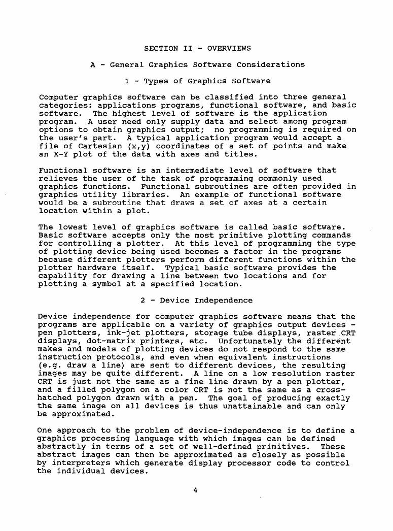
Computer graphics software can be classified into three general categories: applications programs, functional software, and basic software. The highest level of software is the application program. A user need only supply data and select among program options to obtain graphics output; no programming is required on the user's part. A typical application program would accept a file of Cartesian (x,y) coordinates of a set of points and make an X-Y plot of the data with axes and titles.
Functional software is an intermediate level of software that relieves the user of the task of programming commonly used graphics functions. Functional subroutines are often provided in graphics utility libraries. An example of functional software would be a subroutine that draws a set of axes at a certain location within a plot.
The lowest level of graphics software is called basic software. Basic software accepts only the most primitive plotting commands for controlling a plotter. At this level of programming the type of plotting device being used becomes a factor in the programs because different plotters perform different functions within the plotter hardware itself. Typical basic software provides the capability for drawing a line between two locations and for plotting a symbol at a specified location.
2 - Device Independence
Device independence for computer graphics software means that the programs are applicable on a variety of graphics output devices - pen plotters, ink-jet plotters, storage tube displays, raster CRT displays, dot-matrix printers, etc. Unfortunately the different makes and models of plotting devices do not respond to the same instruction protocols, and even when equivalent instructions (e.g. draw a line) are sent to different devices, the resulting images may be quite different. A line on a low resolution raster CRT is just not the same as a fine line drawn by a pen plotter, and a filled polygon on a color CRT is not the same as a cross- hatched polygon drawn with a pen. The goal of producing exactly the same image on all devices is thus unattainable and can only be approximated.
One approach to the problem of device-independence is to define a graphics processing language with which images can be defined abstractly in terms of a set of well-defined primitives. These abstract images can then be approximated as closely as possible by interpreters which generate display processor code to control the individual devices.
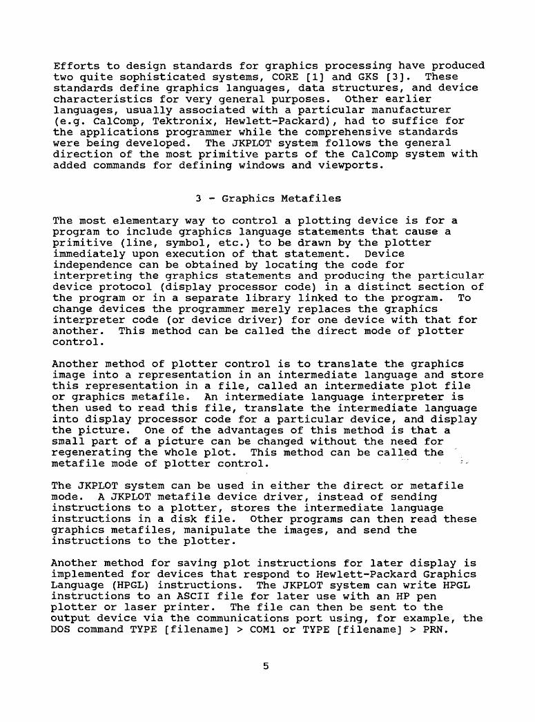
Efforts to design standards for graphics processing have produced two quite sophisticated systems, CORE [1] and GKS [3]. These standards define graphics languages, data structures, and device characteristics for very general purposes. Other earlier languages, usually associated with a particular manufacturer (e.g. CalComp, Tektronix, Hewlett-Packard), had to suffice for the applications programmer while the comprehensive standards were being developed. The JKPLOT system follows the general direction of the most primitive parts of the CalComp system with added commands for defining windows and viewports.
3 - Graphics Metafiles
The most elementary way to control a plotting device is for a program to include graphics language statements that cause a primitive (line, symbol, etc.) to be drawn by the plotter immediately upon execution of that statement. Device independence can be obtained by locating the code for interpreting the graphics statements and producing the particular device protocol (display processor code) in a distinct section of the program or in a separate library linked to the program. To change devices the programmer merely replaces the graphics interpreter code (or device driver) for one device with that for another. This method can be called the direct mode of plotter control.
Another method of plotter control is to translate the graphics image into a representation in an intermediate language and store this representation in a file, called an intermediate plot file or graphics metafile. An intermediate language interpreter is then used to read this file, translate the intermediate language into display processor code for a particular device, and display the picture. One of the advantages of this method is that a small part of a picture can be changed without the need for regenerating the whole plot. This method can be called the metafile mode of plotter control.
The JKPLOT system can be used in either the direct or metafile mode. A JKPLOT metafile device driver, instead of sending instructions to a plotter, stores the intermediate language instructions in a disk file. Other programs can then read these graphics metafiles, manipulate the images, and send the instructions to the plotter.
Another method for saving plot instructions for later display is implemented for devices that respond to Hewlett-Packard Graphics Language (HPGL) instructions. The JKPLOT system can write HPGL instructions to an ASCII file for later use with an HP pen plotter or laser printer. The file can then be sent to the output device via the communications port using, for example, the DOS command TYPE [filename] > COM1 or TYPE [filename] > PRN.

B - Overview of the Software
The JKPLOT system can provide a variety of plotting capabilities with output to a number of different graphics output devices. Not all the capabilities will be required for every application program using this graphics system, and so the system has been segmented into a number of modules to allow a programmer to load only those capabilities necessary. This segmentation, however, makes the resulting list of code modules quite extensive and possibly intimidating to a first-time user. In order that the beginning user not be overwhelmed by the mass of documentation for the JKPLOT plotting programs, a brief overview of the system is provided.
There are two major parts to any plotting system that addresses a variety of graphics output devices: that portion that is independent of the device addressed, and a portion that contains code very specifically tailored to the capabilities of the device. This overview of the JKPLOT system discusses these two parts separately.
1 - Overview of the JKPLOT Device-Independent Code Modulesand Possible Configurations
The device-independent portion of the JKPLOT system consists of five modules which can be configured to provide the minimum level of sophistication necessary for an application programmer's purposes. The names of the modules and a short statement of their functions follows.
JK2DPLT.BAS - This module provides the elementary 2-dimensional plotting instructions for initiating plots and drawing lines and symbols.
2DAX.BAS - Additional capabilities for drawing axes in 2 dimensions and for using scaled plotting instructions are in this module.
JK3DPLT.BAS - Elementary 3-dimensional plotting capabilities and the capability for orienting a plane in 3 dimensions and plotting a 2-dimensional plot on that plane are provided in this module.
3DAX.BAS - Using this module a programmer can specify and draw 3-dimensional Cartesian axes and use scaled plotting commands to draw points and lines.
The four code modules are not independent, but a programmer can select a configuration containing only those modules necessary for the programming task at hand. The size of the code necessary to include all the system capabilities is quite large, so that

the size of an application program loading all four modules is limited. If, however, only the simple 2-dimensional plotting capabilities are required, the application program can be quite large. Table 1 shows four useful configurations of the code modules and the total size (using the size of the disk file storing the module in ASCII form as a measure of size) of each configuration.
REFER TO TABLE 1 - Four configurations and code size totals of the device-independent code modules in the JKPLOT system
Appendix A, Page 1
The plotting functions and subroutines available in each of the five modules are listed in Appendices D to E along with text page references to the detailed description of the commands. The text descriptions explain the meanings of the function and subroutine parameters and demonstrate the use of the commands through detailed examples.
2 - Overview of the JKPLOT Device Dependent Code Modules and Possible Configurations
Each type of output device addressed by the JKPLOT system has its own code module that translates general plot instructions into instructions to cause the device to produce the output desired. These modules are independent, and only those modules necessary for a particular application need be loaded with an application program. The list of modules and devices addressed follows.
QBSCR.BAS - This module provides output for the computer screen.
QBEP.BAS - Output to printers that recognize Epson printer instructions is provided by this module. . >*
QBHP.BAS - Plotters that recognize Hewlett-Packard graphics language (HPGL) instructions can be controlled using this module.
QBLAS.BAS - This module is a minor modification of QBHP.BAS allowing plot instructions to be sent directly a Hewlett-Packard laser printer or saved in an ASCII file for later use.
QBHPF.BAS - Output to an intermediate plot file in HPGL instruction format is provided by this module.
QBJKF.BAS - Plotting instructions in JKPLOT intermediate plot file format are stored to a disk file by this module.
In order that not all the device dependent modules be loaded with an application program that needs only one or two, a code module

that functions as a "traffic-controller" must be constructed and loaded with the applications program. A simple traffic controller, DEVS.BAS, that addresses only the PC screen is included with the plot system, and a program, DEVMAK.BAS, that will construct a controller that addresses only those devices desired by eliminating unwanted lines from the comprehensive "traffic-controller", DEVALL.BAS, is included. Instructions for constructing a specific "traffic-controller" are in section III-JL< 2 .
For applications that will utilize only the JKPLOT intermediate plot file output mode there is a special device driver module, JKFSEP.BAS. Use of this module is explained in Section III-E-3.
C - Overview of the Documentation
The documentation for the JKPLOT system of programs is quite voluminous and includes many tables, figures, program listings, intermediate plot file listings, command summary tables, and example session logs. Including all of the figures, tables, and listings in the body of the documentation would detract from the continuity of the text, and thus an extensive set of appendices was constructed. References to tables, figures, and listings in the text are by appendix letter and page number and are printed in upper case letters at the appropriate place in the text. The reader is advised to locate the referenced material in the appendices when it is first mentioned and have it available while continuing to read the text. All of the figures presented in this report were produced on an Epson printer using the JKPLOT system.
Each of the four device-independent code modules is documented in a separate section of the documentation. In order that the reader be able to construct and execute application programs and examples as soon as possible, the device-dependent code is documented in the section describing the 2D-BASIC plotting routines. This section also explains certain basic graphics ': - concepts necessary for the utilization of the more sophisticated capabilities of the JKPLOT system.
Documentation for the diskettes accompanying this report is compiled separately. A complete list of the directories and files on the diskettes is included in the file README on the disk, and instructions for setting up and using the system on a hard disk (essentially required) is in appendix H.
Certain more sophisticated graphics concepts such as windows, viewports, and 3-dimensional view specifications are described only briefly in the text. The reader is advised to refer to Foley and VanDam [2] for further details.

SECTION III - 2D-BASIC - THE BASIC 2 DIMENSIONALPLOTTING ROUTINES
A - The Basic Plotting System
The unit of measurement for use with the basic plotting system was chosen to be inches. This means that pen position (or pseudo pen position in the case of a CRT) is specified in terms of inches of displacement from a fixed position called the plot origin and that character height is specified in inches. If the user wants to plot a large plot on a CRT screen, the plot can be scaled to fit onto the screen.
The plotting functions included in the basic system were designed to be compatible with a subset of the elementary plotting commands provided with the CalComp Host Computer Basic Software [4], a software package which is supplied with CalComp pen plotters. Names of variables in the programs were chosen to match as closely as possible those used in the CalComp documentation. The names of the standard subroutines, which are described in detail in the following section, are PLOTS, PLOT, NUMBER, SYMBOL, CSYMBOL, POLYLINE, FACTOR, and NEWPEN. An additional command, COMMENT, is included to allow a programmer to include information in an intermediate plot file.
B - The Elementary JKPLOT Instructions
The functions performed by the basic software are described in terms of subroutine calls with arguments.
1. CALL PLOTS(XPAGE, YPAGE, DEVNO%, TKERR%). This routine initializes a plot and is called only once (before a call to any other graphics subroutine). Execution of this command opens the plot output device through the computer's operating system, performs scaling calculations, and sets the clipping window. Values of X (the horizontal coordinate) will be clipped at 0 and XPAGE, and values of Y (the vertical coordinate) will be clipped at 0 and YPAGE. The variable, DEVNO%, specifies the output device, and TKERR% returns a FALSE (0) value if no error has occurred while executing the PLOTS command and a TRUE (-1) value if an error has occurred. Table 2 shows shows the numerical codes for the devices addressed by the JKPLOT system in the form of "defined constants" that can be used in a program. The constants are defined in the include file, "JK2DCOM.INC".
REFER TO TABLE 2 - Numerical codes and defined constants for JKPLOT output.
Appendix A, Page 1

2. CALL PLOT(X, Y, P%). This is the basic pen movement command. X and Y are coordinates, in inches, from the current reference point (origin), of the position to which the pen is to be moved, and P% is a signed integer which controls the pen status (up or down) and origin definition.
If P% = 2 the pen is down during movement, thus drawing a visible line. If P% = 3 the pen is up during the move.
If P% = -2 or -3, a new origin is established at the terminal position after movement is completed as if P% were positive. In this case the logical X,Y coordinates of the new pen position are set equal to zero, and this position is the reference point for succeeding movements. If P% = 999 the effects are the same as if P% were -3 except that the plot is terminated and the output device is closed. The values of X, Y, and P% are not changed by this subroutine call. Values of P% other than those described default to P% = +3.
3. CALL SYMBOL(X, Y, HT, TXT$, ANGLE). This is the standard routine for plotting text character(s) as specified by the variable TXT$. The pen is first moved to the position specified by X and Y. This is the location of the lower left corner of the first character to be plotted. The size of the character(s) in inches is specified by HT, and ANGLE specifies the angle, in degrees from the positive horizontal axis, at which the text is to be plotted. If ANGLE = 0 the text will be plotted right side up and parallel to the horizontal axis. The text in the character variable TXT$ may consist of any of the characters listed in Figure 1. If a character not in the acceptable character set is included in TXT$ a blank is plotted in its place. The length of the text in plot inches can be calculated by using the fact that each letter is exactly as wide as it is high. Hence a string of ten characters plotted with a height of 1/4 inches would be 2.5 inches long.
The JKPLOT system gives the user a choice of eight character '- fonts for use with the SYMBOL subroutine. The definitions of the fonts are in eight separate files named JKFONT.X, where the X stands for a digit between 0 and 7 inclusive. Any font used must be present in the working directory. The ASCII code for each of the characters in the fonts, the font numbers, and the font names are shown in Figure 1.
REFER TO FIGURE 1. - JKPLOT character fonts for standard SYMBOL call
Appendix B, Page 1
The default font is font number 0, which is reinitialized any time the PLOTS subroutine is called. If the user wants to change fonts the subroutine NEWFONT(fontnumber%) can be used. The font
10

number must be an integer between 0 and 7. For example, to set the font to number 3, TRIPLEX, the user can issue the command
CALL NEWFONT(3).
4. CALL CSYMBOL(X, Y, HT, Q%, ANGLE, PENUP%). This is the centered symbol routine and is used to draw special centered symbols such as boxes, octagons, rectangles, etc., for plotting data points. The pen is first moved to the position specified by X and Y. This is the location of the center of the symbol to be drawn. If the variable PENUP% contains the value -1 the pen is up during the move, and if the value of PENUP% is 0 the pen is down during the move. The height of the symbol in inches is specified by the variable HT, and the rotation in degrees of the symbol about its center is specified by the variable ANGLE. The symbol to be plotted is specified by the value of Q%, which must take a value between 0 and 13. The symbols corresponding to the values of Q% are listed in Figure 2.
REFER TO FIGURE 2. - Symbols for centered CSYMBOL call Appendix B, Page 5
The centered symbol font definitions are in a file named JKCFONT.O, which must be present in the working directory. In the present version of the JKPLOT system there is only one file for centered character fonts. However, in order to allow a user to expand the file of centered fonts or to use a different set of fonts the subroutine NEWCFONT(cfontnumber%) has been included. At present the only acceptable number for the parameter cfontnumber% is 0.
5. CALL NUMBER(X, Y, HT, FPN, ANGLE, NDEC%). This routine causes the floating point number in the variable, FPN, to be plotted in decimal format. The meanings of the arguments X, Y, HT, and ANGLE are the same as those described for the subroutine SYMBOL. The integer value in NDEC% specifies the format and precision of the number to be plotted. If NDEC% is greater than 0 it specifies the number of digits to the right of the decimal point that are to be converted and plotted after appropriate rounding. For example if the value in FPN is 12.3456 and NDEC% is +2, the number plotted would be 12.35. If NDEC% = 0 only the number's integer portion and a decimal point are plotted after rounding. If NDEC% = -1, only the number's integer portion is plotted, after rounding, and if NDEC% is less than -1, -NDEC%-1 digits are truncated from the integer portion after rounding. If FPN= 143.2 and NDEC%= -2 then the number 14 would be plotted.
6. CALL POLYLINE(XARY(), YARY(), NPTS%, INC%, LINTYP%, Q%, HT). The POLYLINE subroutine produces a line plot of the pairs of data values in the arrays XARY() and YARY() with centered symbols plotted at some of the data points as specified by the parameters
11

LINTYP% and INC%. The symbol to be drawn is specified by the value of Q% (with the same meaning as in the CSYMBOL call), and the size of the symbol is specified by HT.
The pen is first moved to the position specified by XARY(l) and YARY(l) in the up position. The value of the integer variable, LINTYP%, indicates the type of line to draw through the data points. If LINTYP% = 0 the points are connected by straight lines, but no symbols are drawn. If LINTYP% is negative, no line segments are drawn; only the symbols are plotted, and if LINTYP% is positive, both the line and the symbols are drawn. The magnitude of LINTYP% specifies the frequency of plotted symbols. For example if LINTYP% = 4 a symbol is plotted at every fourth data point. The value of INC% specifies the number of points to use for defining the line. For example if INC% = 4 every fourth point is used as a line segment endpoint; the three intermediate points are ignored. Examples of type of line drawn for selected values of the parameters LINTYP% and INC% are shown in Figure 3.
REFER TO FIGURE 3. - Examples of type of line drawn for selected values of the parameter LINTYP% and INC%
Appendix B, Page 5
7. CALL NEWPEN(PN%). If the plotter being used has the capability of using more than one pen, this call will specify which pen is to be used in subsequent plotting system calls. The value of PN% is initialized to 1 by the initial call to PLOTS.
The JKPLOT system sets a special color palette for the PC EGA and VGA screens. Symbolic constants are defined in the include file, JK2DCOM.INC, and are listed in Table 3.
REFER TO TABLE 3 - Defined constant and symbolic values for use with the NEWPEN command ' -
Appendix A, Page 2
The Hewlett-Packard laser printer can plot in only one color, but there is the capability for varying line widths. In order to take advantage of this capability the number of pens defined for the laser printer in the device dependent code module, QBLASER.BAS, is nine. The default pen, number 1, is set for a line width of .2 millimeters, and the pen thicknesses for pens numbered two through nine can be calculated in millimeters using the formula
line thickness = .05 * (pen number).
12

8. CALL FACTOR(FACT). The factor subroutine causes all subsequent pen movements to be enlarged or reduced by a factor, FACT. If FACT =2.0 the plotting movements will all be twice normal size, and if FACT = 0.5 the movements will be half normal size. FACT is initialized to 1.0 by the initialization call to PLOTS.
9. CALL COMMENT(CMT$). This routine causes no plotting. It is included so that comments can be sent to the plotting system. Some possible uses of this command are to send information about the progress of a plot to the PC screen when the output device is a printer to include information about the function being performed in an intermediate plot file being generated.
10. CALL SetFnam(DEVNO%, FILNAM$). This routine specifies the file name for intermediate plot file output and must be called before the initialization call to PLOTS. DEVNO% is the device number and can be either JKFIL, HPFIL, or LSFIL. FILNAM$ is the name of the intermediate plot file to be generated.
REFER TO TABLE 4 - Summary of standard calling sequences Appendix A, Page 3
C - Expanded Font Tables and Environmental Variables
The sequences of pen strokes defining each character in the fonts are stored in disk files with names JKFONT.O - JKFONT.7 for the standard symbol call and JKCFONT.O for the centered symbol call. These files have a complex structure for defining the sequence of characters, but a knowledgeable user can append additional symbols to existing fonts or define completely new fonts. An explanation of the font file structure and an example of adding a new symbol to the centered symbol font set are in Appendix I.
When the JKPLOT system is initialized (e.g. with use of the PLOTS subroutine) or when a request to change fonts is received (via the NEWFONT or NEWCFONT subroutines) the program by default attempts to locate and read the desired font file in the current working directory. The font files must thus be available at execution time, and if work is being done in a number of different directories the font files must be reproduced in each of these directories. The need for these multiple copies of the font files can be avoided by using an environmental variable, JKPLT.
If a user has a number of regularly used programs utilizing the JKPLOT system, a reasonable way to be able to access all of them from any working directory without having to make multiple copies is to keep them in a single graphics directory. The operating system can then be informed of their location through the use of
13

the PATH command. For example if the DOS system programs are kept in a directory named C:\DOS and the graphics programs are stored in a directory named C:\JKPLOT\EXEC, the user can execute the DOS command
PATH=C:\DOS;C:\JKPLOT\EXEC
to tell the operating system where to find the graphics programs. This command alone will not tell the system where to find the font-definition files, and copies of these files will have to be in the current working directory.
The user can, however, use the DOS command
SET JKPLT=C:\JKPLOT\EXEC\
to define an environmental variable, JKPLT. The JKPLOT programs will then use the directory thus specified to locate the font files, eliminating the need for multiple copies of these files.
D - Default Scaling
There are two procedures used in default mode for scaling a picture. Because the actual size of a picture produced on the PC screen depends on the size of the monitor, the term "plot inches" is not meaningful for these devices. Default calculation for this driver scales the plot to produce the largest aspect- preserving image that can be drawn on the CRT screen. The aspect ratio of a rectangle is the ratio of the width to the height. Without aspect-preservation a square might be drawn as a tall, thin rectangle. For "inch-type" plotters, i.e. devices for which the term "plot inches" is meaningful (HP plotters and Epson printers), the plot produced is the size specified by the parameters XPAGE and YPAGE unless the plot scaled this way would be too big for the plotter. In this case a warning flag is set in the plotting system, and the plot is scaled to a size that-, will fit on the plotter.
E - Structure and Use of the JKPLOT Device Drivers
1 - Direct vs. Metafile Mode
There are two elementary ways to use the plot drivers described in this paper. The most direct way is to write a program in QuickBasic, calling the plotting routines described in Section I. The plot system configured for the specific plotting devices used by the program can then be linked with this program, and when the program is executed, the plot will be drawn on the output device. Another way is to write the same QuickBasic program but link the a special version of the plot system configured to generate intermediate plot files. This procedure will produce an intermediate plot file of Calcomp-like commands. The
14

intermediate plot file is an ASCII file containing on each line the name of the plot subroutine to be called along with the parameter values to be set before transfer to the plot subroutines.
Each method of using the plotting system has advantages. The method that sends the output directly to the plotting device has the advantage of immediacy; the product of the program is immediately available for viewing when the program is run. On the other hand, the method that uses the intermediate plot file allows the user to make a number of plots with the same page size and then send them all to the plotter at the same time - a system for overlaying individual plots. The knowledgeable user can also use a standard ASCII file editor to change aspects of a plot by editing the intermediate plot file. Examples of both of these methods will be given in the following sections.
2 - Code Modules for Direct Mode Plotting
The bulk of the basic plotting system code is independent of which output device is to be addressed. This code is in a module named JK2DPLT.BAS. This module does all of the 2-dimensional scaling and transformation calculations and contains the character generator, which calculates the individual pen strokes necessary to draw a character. Except for device opening and closing and pen change instructions, the JK2DPLT.BAS module routes all plotting instructions through a subroutine that tells a device to draw a straight line from one point to another.
The instruction to draw a line from one point to another is sent to a "traffic director" module which directs the instruction to the device-specific code for whichever device is being addressed. The device-specific code for each device is contained in a separate module which directly controls the device, and "traffic director" module allows for the presence of more than one device -specific module in a program. The devices and corresponding module names are listed in Table 5. Note that the JKPLOT ~'>,. intermediate plot file output obtained when using the device- specific module QBJKF.BAS is not the most efficient way to store a plot because all symbols and numbers to be plotted are stored in the file as sequences of line segments. A more efficient method for generating and storing plots in an intermediate plot file is described in Section III-E-3.
REFER TO TABLE 5 - Device specific code for plot drivers Appendix A, Page 4
Because of the way the the linker functions, different versions of the "traffic director" module must be constructed for each combination of device drivers to be loaded. If all devices are to be available to the applications program, the complete
15

"traffic director" module, DEVALL.BAS, can be used. Use of DEVALL.BAS causes the linker to load all of the device-specific modules listed in Table 5. However loading all the drivers when only one is needed by a program uses valuable program code space in the computer memory, and so it is worthwhile to be able to construct smaller versions of the "traffic director" module which address a specific subset of the devices.
The JKPLOT system includes a program, DEVMAK.BAS, which will construct the needed smaller versions of DEVALL.BAS by removing all program lines that are concerned with devices to be omitted. This program instructs the user to input a sequence of six numbers, each 0 or 1 and separated by commas, via the keyboard. The six numbers indicate to the program which device-specific code modules to include, a 1 indicating inclusion and a 0 indicating exclusion. The devices corresponding to the six positions in order are the PC screen, HPGL pen plotter, Epson printer, HPGL file output, JKPLOT intermediate plot file output, and laser printer output. For example the sequence 1,0,1,0,0,0 indicates that the PC screen and the Epson printer device modules are to be included.
The name of the output program file constructed by the DEVMAK.BAS program depends upon the devices included. The base of the file name for all possibilities is DEVxxxxx.BAS, where the x's represent single letters or blanks indicating which devices are included. The single letters are "S" for the PC screen, "H" for the HPGL plotter, "E" for the Epson printer, "P" for an HPGL plot file, "K" for a JKPLOT intermediate plot file, and "L" for laser printer output. For example the name of the file produced in response to tfie input sequence 1,0,1,0,0,0 would be DEVSE.BAS. If the sequence 1,1,1,1,1,1 is inserted the program informs the user that the module "DEVALL.BAS" is available for addressing all the devices.
The device "traffic director" includes two routines which may be accessed by the user directly for use in application programs-but which are not actually part of the standard plot system. The first is a subroutine, DEVLST(ndev%, lst%(), lst$(), echr%()), to return a list of the devices loaded (as determined by the version of DEVALL.BAS used) in a particular program. The parameters returned by the subroutine are
ndev% the number of devices availablelst%() an integer array containing a list of the JKPLOT
coded device numbers (see table 2) lst$() a character array containing abbreviated names
of the available devices (for possible use witha menu system)
echr%() an integer array containing the index of acharacter in the corresponding entry of the lst$()array so that a menu system can recognize theentry using a single character.
16

The second extra routine is the function, VideoHardware%(), which interrogates the operating system to find out what graphics board/monitor combination is present. This routine can identify, for example, the presence of an EGA graphics board being used with a monochrome monitor. The function returns the JKPLOT system coded device number (see table 2), through the use of the INTERRUPT instruction. Programs that use the INTERRUPT instruction require that the QuickBasic interpreter be initialized using the /I option (specifying the use of the Quick library distributed with QuickBasic), and that compiled programs be linked using the QuickBasic library (QB.LIB).
A complete program would consist of the application program, the device independent code in JK2DPLT.BAS, a version of the "traffic-controller" DEVxxxxx.BAS, and the device-specific code modules for each of the devices addressed by DEVxxxxx.BAS. If the application program name is APP.BAS, a batch file for compiling and linking this program with the plot system to use the PC screen and the Epson plotter would contain the instructions
BC APP.BAS /AH/X/O;BC JK2DPLT.BAS /AH/X/O;BC DEVSE.BAS /AH/X/O;BC QBSCR.BAS /AH/X/O;BC QBEP.BAS /AH/X/O;LINK APP+JK2DPLT+DEVSE+QBSCR+QBEP,,,qb.lib;
Execution of this batch file produces an execution module named APP.EXE. To execute the program the user must enter APP via the keyboard.
To run the program from within the QuickBasic environment a user would first open the file APP.BAS and then load the remaining four programs shown in the example batch file. The program could then be run using the QuickBasic "RUN" option.
The device independent code module JK2DPLT.BAS and all of the device specific drivers listed in Table 5 can be put into a plot system library, and by accessing this library the commands necessary to compile and link an application program can be greatly simplified. Construction and use of the plot system libraries is discussed in section III-I.
3 - Metafile Mode
To use the plot system in metafile mode, the user can link a special version of the plotting system, in a module called JKFSEP.BAS, with the applications program. The resulting program can then be executed through the interpreter or compiled. The result of executing this code is a disk file containing the intermediate language instructions for drawing the plot. The
17

special version of the plot system produces a much more compact intermediate plot file than the integrated file-producing module QBJKF.BAS. JKFSEP.BAS just writes the name of the called subroutine along with the relevant parameters to the output file. In addition the code required for file output is much less than the code needed for the complete plotting system, and much larger applications programs can thus be implemented. The metafile driver, JKFSEP.BAS, contains entry points for all the JKPLOT functions and subroutines, but only the CalComp-like instructions will be discussed in detail because these instructions can easily be modified in the intermediate plot file. The more sophisticated routines do not lend themselves to plot file modification. Table 6 lists the basic plot system calls and the corresponding lines written to the intermediate plot file with an example for each command. Lines labeled C: are the subroutine calls and lines labeled F: are the corresponding lines written to the plot file. A complete list of all the JKPLOT system functions and subroutines with the corresponding form for intermediate plot file output is in appendices F and G.
REFER TO TABLE 6 - Examples of intermediate plot file output for JKPLOT subroutine calls
Appendix A, Page 5
A batch file for compiling and linking an application program, APP.BAS (APP.BAS is a hypothetical program name, not a program supplied with the JKPLOT system), with JKFSEP.BAS is
BC APP.BAS /AH/X/0; BC JKFSEP.BAS /AH/X/O; LINK APP+JKFSEP;
Note that there is no need to specify the QuickBasic library, QB.LIB, in this link command because no version of the "traffic director" module, DEVALL.BAS, is used. This batch file will ^ produce an execution module named APP.EXE which can then be executed by entering APP via the keyboard.
To run the program from within the QuickBasic environment a user would first open the file APP.BAS and then load JKFSEP.BAS. The program could then be run using the QuickBasic "RUN" option.
In order to send the stored plot to a particular device, a program that reads the plot metafile and sends the proper device protocol to the device must be constructed by merging a file- reading application program with the appropriate device driver described above. A file-reading application program, QF1.BAS, is supplied with the JKPLOT system. With this program a user can read up to ten plot files with the same page size, select a viewing window, select a viewport, rotate the plot, and then send the resulting image to a particular device.
18

4 - Configuration Files
The device-specific code modules for the Epson printer, the HPGL pen plotter, and the Hewlett-Packard laser printer require the presence of configuration files named CONFIG.LPT, CONFIG.HP, and CONFIG.LAS to be present in the working directory in order to set proper communications between the computer and the plotting device. The files contain a single line of text enclosed in quotes. For the HPGL plotter configuration file the text line specifies the asynchronous transmission port that the device is attached to, the transmission speed (baud), and other parameters that apply to communication between a hardware device and the computer. The user is referred to the OPEN COM .. statement in the IBM Basic manual for explanation of these parameters. The file CONFIG.HP included on the JKPLOT diskette contains the line (including the quotation marks)
"COM1:2400,N,8,1,RS,CS65535,DS,CD"
The configuration files for the Epson printer and Hewlett-Packard laser printer are used to allow the user to specify either LPT1 or LPT2 as the output device. The files CONFIG.LPT and CONFIG.LAS included with the JKPLOT diskette contain the line (including the quotation marks)
"LPT1:"
The configuration files can be stored in a directory other than the working directory if the user sets the an environmental variable, JKPLT, as described in section III-C.
F. - Examples Using the Elementary Plot System
For the following examples it will be assumed that the user has constructed a PC VGA screen driver module, DEVS.BAS, by executing the program DEVMAK.BAS and responding to the input query with the sequence 1,0,0,0,0,0. The DEVS.BAS program can be compiled, \, resulting in the object module DEVS.OBJ, by executing the command line "be DEVS.BAS /ah/x/o; 11 . Both the source and object module should be available in the working directory so that the example can be either compiled or executed from within the QuickBasic programming environment. It will also be assumed that the source and object modules, JKFSEP.BAS and JKFSEP.OBJ, and the include files, JK2DPLT.INC, JKPLTTYP.INC, JK2DCOM.INC, and JK2DINT.INC, are available in the working directory. These include files contain, among other things, the defined numerical constants for the output devices and the function and subroutine declaration statements for the plot system. The application program must have the "include" metacommand
' $INCLUDE: 'JK2DPLT.INC'
at the beginning of the program.
19

1 - Example 1
The first example plot is very simple one. The plot consists of a 5 inch by 5 inch square box with the message, EXAMPLE 1, in .25 inch letters centered in the box. The program EXAMPLEl.BAS, which will produce this plot and draw the figure on the PC screen is in appendix C. Comments within the program explain what is being accomplished by the code.
REFER TO EXAMPLEl.BAS - Program to produce figure 4. Appendix C, Page 1
The program modules used for example 1 are EXAMPLEl.BAS, JK2DPLT.BAS, DEVS.BAS, and QBSCR.BAS. The result of running this program is shown in Figure 4.
REFER TO FIGURE 4 - An elementary example showing the use of the JKPLOT system. (size reduced)
Appendix B, Page 6
In the program, EXAMPLEl.BAS, the output device is specified by a program variable, devno%, which is set using the VideoHardware%() function discussed in Section III-E-2. The program line
devno% = VideoHardware%
accomplishes this definition. By changing this program line to
devno% = EPSHR
the output can be directed to the Epson printer in high resolution mode. The program modules necessary to execute the^ program then become EXAMPLEl.BAS, JK2DPLT.BAS, DEVE.BAS, and QBEP.BAS.
Another way to generate the picture on the PC screen is create a JKPLOT intermediate plot file and then use the file-reading plot driver, QF1.EXE, to send the plot to the screen. In order to use this method the source code in the program EXAMPLEl.BAS must be slightly modified by replacing the code line
devno% = VideoHardware%
with the two lines of code
devno% = JKFILCALL SetFnam(devno%,"EXAMPLEl.PLT")
20

Note that the output intermediate plot file name, EXAMPLEl.PLT, must be specified before the initialization call to PLOTS. The user can make the program modification after entering the QuickBasic programming environment using the QuickBasic editing commands. The program modules necessary to create example 1 in this mode are EXAMPLE1.BAS and JKFSEP.BAS. When the program is run the result will be the intermediate plot file, EXAMPLE1.PLT, listed in Appendix D and containing a list of CalComp-like commands. This intermediate plot file can then be sent to the PC screen or another output device by executing the program QF1.
REFER TO EXAMPLE1.PLT - Intermediate plot file for figure 4. Appendix D, Page 1
A third way to generate the above plot is to use a file editor such as EDLIN to create the intermediate ASCII plot file, EXAMPLE1.PLT, directly. The user can then execute the program QF1, and the image will appear the screen. If the user understands the construction of the intermediate plot file, many plot modification possibilities are available.
2 - Modification of an Intermediate Plot File
An intermediate ASCII plot file is just a sequence of CalComp- like instructions that can be read by a program like QF1. Hence the user can insert plot commands or move images by proper modification of the file. This capability is very valuable if the user has constructed a large, complicated plot and just wants to make a few changes or to add extra documentation without regenerating the whole file.
For example, addition of the line
SYMBOL, 0,1.5,1,.25,0,MODIFIED
immediately after the SYMBOL call in the intermediate plot file for Example 1 causes the text, "MODIFIED", to appear below the original text in the figure, producing the plot shown in Figure 5.
REFER TO FIGURE 5 - An example showing the result of modifying the intermediate plot file for Figure 4. (size reduced)
Appendix B, Page 6
21

3. - Example 2
The program, EXAMPLE2.BAS, demonstrates the use of most of the elementary commands available in the basic plotting software. The program modules necessary for example 2 are EXAMPLE2.BAS, JK2DPLT.BAS, DEVS.BAS, and QBSCR.BAS.
REFER TO EXAMPLE2.BAS - Program to produce figure 6. Appendix C, Page 2
An intermediate plot file can be produced by running the program in metafile mode.
REFER TO EXAMPLE2.PLT - Intermediate plot file for figure 6. Appendix D, Page 2
Figure 6 shows the resulting plot.
REFER TO FIGURE 6 - An example showing the use of most of the elementary commands available in the JKPLOT system (size reduced).
Appendix B, Page 7
G - Windows, Viewports, and Clipping
Such graphics concepts as windows, viewports, aspect ratios, clipping, and pipelines are defined only superficially in this paper. The reader is referred to Foley and VanDam [2] for a more definitive discussion.
1 - Normalized Device Coordinates (NDC) >.
In order that the JKPLOT system be able to produce graphics on a variety of different output devices using the same plotting commands it is necessary to define a logical coordinate system that represents the plotting surface in a device independent manner. This coordinate system can be thought of as a virtual or normalized device on which the graphics output is initially drawn, and the coordinates are called normalized device coordinates (NDC). The normalized device coordinates defining the graphics image (NDC image) are then transformed to device coordinates, which differ significantly from one device to another. For example the PC VGA screen has horizontal coordinate limits of 0 through 639 and vertical coordinate limits of 0 through 359 while the Epson high resolution printer with an eight inch carriage has horizontal limits 0 through 959 and vertical limits of 0 through 2159. The normalized coordinate system
22

chosen for the JKPLOT system is defined in plot inches to correspond to the elementary Calcomp-like commands.
The default size of the plotting surface on the conceptual normalized device is specified (in units of inches) by the parameters XPAGE and YPAGE in the initialization call using the PLOTS subroutine. Note that this definition of normalized device coordinates is different from that used by Foley and Van Dam [2] and by the GKS [1] system, both of which define the normalized device coordinate limits to be from 0 to 1 in both the horizontal and vertical directions.
The device plotting surface limits, which may be called work station limits, are determined by the parameter DEVNO% in the PLOTS call. Execution of the PLOTS subroutine causes the plot system to set the plotting surface limits and to calculate the transformation relating the normalized device (inch) coordinates to those of the output device. The rectangular region in normalized coordinate space, with default definition specified by XPAGE and YPAGE, is called the work station window, and the rectangular surface defined on the output device, which by default is the whole device surface, is called the workstation viewport. The transformation relating NDC coordinates to device coordinates is called the work station map and is part of a more complex transformation structure call the work station pipeline, which will be defined later.
2-2 Dimensional World Coordinates
A user may be interested in plotting an image or graph that does not use inches as the elementary coordinate measure. For instance a geologist might want a plot of percent gold against percent silver in a set of samples, or a mining engineer might want to plot profit in dollars against extraction block size for an open pit mine. These application or user-oriented coordinates are naturally called user coordinates or world coordinates. In order to accommodate such applications another conceptual ^ plotting surface, along with a corresponding coordinate system, is defined within the JKPLOT system. This plotting surface is called the world coordinate surface, and the transformation relating world coordinates to normalized device coordinates is called the world coordinate map. The world coordinate map is part of a more complex structure called the world coordinate pipeline. The default definition of the world coordinate plotting surface (the default world coordinate window) is exactly the same as the default normalized device coordinate surface, and the default world coordinate map is just the identity map. The rectangular region in normalized device coordinate space onto which the world coordinates are mapped is called the world coordinate viewport. Figure 7 shows the default sequence of figures for a duck drawn in world coordinates, normalized device coordinates, and screen coordinates.
23

REFER TO FIGURE 7 - Sequence of images showing a duck in world coordinates, normalized device coordinates, and screen coordinates under default plot system settings.
Appendix B, Page 8
3 - General Window to Viewport Mappings
In world coordinate space a rectangular region containing the information the programmer wants displayed is called the world coordinate window, and the rectangular region in plot inches (NDC) onto which this information is to be mapped is call the world coordinate viewport. The plotting system calculates the world coordinate map which transforms the world coordinates into plot inches. Another rectangular region, different from the world coordinate viewport, in NDC space can be selected for display on the output device. This region is called the work station window, and the rectangular region selected on the output device plotting surface for display of the information in the work station window is called the work station viewport. The mapping relating plot inches to device coordinates is called the work station map. Figure 8 shows a sequence of images of a duck in world coordinates, normalized device coordinates, and screen coordinates with a world coordinate window, work station window, and work station viewport selected.
REFER TO FIGURE 8. - Sequence of images of a duck in world coordinates, normalized device coordinates, and screen coordinates with a world coordinate window, work station window, and work station viewport selected.
Appendix B, Page 8
The two maps, world coordinate and work station, are not calculated in exactly the same manner. The work station map -- calculates the coordinate mapping between plot inches and device coordinates in such a way that the aspect ratio of the work station window is preserved. The aspect ratio of a rectangle is the ratio of the vertical extent of a the rectangle to the horizontal extent of the rectangle. An aspect preserving mapping would, for example, map a square window into a square image. For non-plot inch type displays such as the PC screen the work station map is calculated, in default mode, to display the largest aspect-preserving image that will fit in the work station viewport, with the lower left corner of the window mapped into the lower left corner of the viewport. There are plot system switches that allow the programmer to specify that the image be centered in the viewport or rotated within the viewport. For plot inch type devices such as the Epson printer or an HPGL plotter the work station map locates the image in the lower left corner of the viewport and plots the image to proper scale. If
24

the plot is larger than the specified viewport the scaling proceeds as if the device were a non-plot inch device.
The world coordinate map is not defined to be aspect preserving. This means that if a tall, thin rectangular region in world coordinate space is specified as the world coordinate window and a short, wide rectangle is specified as the world coordinate viewport, the shape of the world coordinate image will be made shorter and wider to fill the world coordinate viewport. In order for the world coordinate map to be aspect-preserving the aspect ratios of the world coordinate window and the world coordinate viewport must be the same. Figure 9 shows a sequence of images of a duck in world coordinates, normalized device coordinates, and screen coordinates with a world coordinate viewport half as high as the world coordinate window.
REFER TO FIGURE 9. - Sequence of images of a duck in world coordinates, normalized device coordinates, and screen coordinates with a world coordinate viewport half as high as the world coordinate window.
Appendix B, Page 9
The programmer can specify the windows and viewports with the following functions defined in the JKPLOT system.
FUNCTION SetWcWin%(l, r, b, t) 'world coordinate windowFUNCTION SetWcVp%(l, r, b, t) 'world coordinate viewportFUNCTION SetWsWin%(l, r, b, t) 'work station windowFUNCTION SetWsVp%(l, r, b, t) 'work station viewport
The arguments 1, r, b, and t of these functions are the left, right, base, and top coordinates respectively of the rectangle being defined. For the function SetWcWin% the arguments are in world coordinates. For the functions SetWcVp% and SetWsWin% the arguments are in plot inches, and for SetWsVp% the arguments are in device coordinates. A programming example showing the use of these functions is in Section III-G-6.
In summary, in order to specify the coordinate mapping between world coordinates and plot inches the user specifies a world coordinate window and a world coordinate viewport. The default rectangles for the world coordinate window and the world coordinate viewport are the rectangle with horizontal limits 0 and XPAGE and vertical limits 0 and YPAGE. In order to specify the coordinate mapping between plot inches and device coordinates the user specifies a work station window and a work station viewport. The default work station window is the rectangle with horizontal limits 0 and XPAGE and vertical limits 0 and YPAGE. The default work station viewport is the whole output device plotting surface.
25

4 - Clipping
The window/viewport combination defines a mapping of coordinates from one coordinate space to another. The graphics image to be transferred may, however, extend beyond the boundaries of the window. By default any portion of the image that does not lie within the window is clipped before being mapped to the viewport. If coordinates outside the window are not clipped the image displayed might vary from device to device because different devices respond differently to coordinate specifications outside their normal range.
The user can specify a clipping rectangle other than the default using the function SetClip%(wch$, 1, r, b, t). The argument, wch$, specifies which pipe the clipping rectangle is to be associated with. Wch$ can take on the values "WS" or "WC", specifying work station or world coordinate respectively. If wch$ = "WS" then the rectangle specified by left, right, base, and top values of 1, r, b, and t respectively will be used for the work station clipping rectangle instead of the work station window. If the value of wch$ is "WC" then the specified rectangle replaces the world coordinate window as the clipping rectangle.
Clipping in either the world coordinate or the work station pipe can be turned off with the function ResetClip%(wch$). The parameter wch$ can take on either of the values "WS" or "WC". A programming example showing the use of the clipping functions is in Section III-G-6.
5-2 Dimensional Transformations
Some graphics applications may require a sequence of views of the same object to be drawn or may require that an object easily defined in one location be displayed in another. These goals can be accomplished in the JKPLOT system using the following 2 : dimensional transformation subroutines: '-
SUB Eval2dTran(fx, fy, tx, ty, rot, sx, sy, mat()) SUB SetTrn2(wch$, mat()) SUB AcmTrn2(wch$, mat()).
The subroutine Eval2dTran calculates a transformation matrix which can then be used to set a transformation with SetTrn2 or accumulate a transformation with AcmTrn2 in either the world coordinate or work station pipes. Fx and Fy are the fixed point; tx and ty are the translation or shift vector; rot is the angle of rotation in degrees; and sx and sy are the scale factors. The transformation matrix is returned in the 4x4 matrix mat(). This matrix can then be used to set or accumulate the transformation in world coordinates or normalized device coordinates depending upon whether the parameters wch$ is set to "WC" or "WS".
26

The transformation is computed so that the order of transformation operations is scale, rotate translate. Figure 10 illustrates this sequence applied to a duck using the following program statements to set the transformation in world coordinates:
Call Eval2dTran(3,8.8,10,-5,45,.5,. 5,mat()) call SetTrn2("WC",mat()).
REFER TO FIGURE 10. Sequence of images of a duck showing the order of operations to complete a transformation.
Appendix B, Page 10
6 - World Coordinate and Work Station Pipes
Each of the coordinate calculations, from world coordinates to plot inches and from plot inches to device coordinates, is accomplished by the same sort of structure. This structure, which may be call a pipeline step, consists of a 2 dimensional transformation, a clipping rectangle, and a 2 dimensional mapping. The JKPLOT system has two pipeline steps, the world coordinate pipe and the work station pipe. The complete pipeline sequence is shown in Figure 11.
REFER TO FIGURE 11. The complete 2-dimensional JKPLOT pipeline Appendix B, Page 10
Figure 12 shows the cumulative effect of transformations, clipping rectangles, windows, and viewports as an image of an octagon is passed through the JKPLOT pipeline. Each pipeline shown in the figure represent the sequence of images in the pipeline under the cumulatively more complex manipulations specified for the pipeline. '--
REFER TO FIGURE 12. Images of an octagon as it is passed through the JKPLOT pipeline under cumulatively more complex operations.
Appendix B, Page 11
The program, EXAMPLES.BAS, will generate the final image of the octagon shown in Figure 12 for each of the seven steps. The program modules necessary for example 3 are EXAMPLES.BAS, JK2DPLT.BAS, DEVS.BAS, and QBSCR.BAS.
REFER TO EXAMPLE 3.BAS - Pipeline demonstration program. Appendix C, Page 5
27

H - Using Special JKPLOT System Switches
One of the variables defined and placed in COMMON in the include file JK2DCOM.INC is a structured variable describing the present state of the plotting program. This variable, with base name ST, can be used by a knowledgeable programmer to interact directly with the plot system. The three most useful switch variables are ST.NOEQASP, ST.CLPCEN, and ST.PICROT. Each of these variables is normally in the off (FALSE OR 0) state but when set to TRUE OR -1 by a programmer causes slightly different calculations to be done in the plot system.
If ST.NOEQASP is set to TRUE the work station map calculation stretches the image of the work station window to fill the work station viewport in both the horizontal and vertical directions. The work station map by default is aspect-preserving, which means that if the aspect ratio of the window and viewport are not the same, some of the viewport will not be used. The default calculation places the image of the window in the lower left corner of the viewport in this case.
If ST.CLPCEN is set to TRUE the work station map calculation locates the image of the work station window in the center of the work station viewport rather than in the lower left corner.
If ST.PICROT is set to TRUE the whole plot is rotated on the output device by reversing the horizontal and vertical axes of the plot. This switch is useful when a user wants to send a tall, thin plot to a device that has a short, wide plotting surface.
To set the switches the user must first complete the plotting system initialization using a call to the PLOTS subroutine. The PLOTS subroutine sets the switches to default status (off or FALSE). The user can then execute the following example code segment (using ST.PICROT for the example) to give a switch a TRUE value and cause the plotting system to recalculate the work '- station mapping transformation.
ST.PICROT = -1 'true Call CalcWsMap.
Further examples of the use of the plotting system switches are in the program QF1.BAS in which the author has made significant use of all the switches.
Figure 13 shows the default position of a simple square plot drawn on the screen with all the switches off and then the effect of setting each switch on before sending the plot to the screen.
28

REFER TO FIGURE 13 - Effect of JKPLOT system switches Appendix B, Page 12
I - Constructing a JKPLOT System Library
1 - Stand-Alone Libraries
If a programmer is going to need the JKPLOT routines regularly a library can be constructed in order to avoid recompiling and explicitly linking individual modules. The device independent module, JK2DPLT, and all of the device-specific modules, QBSCR, QBEP, QBHP, QBJKF, and QBHPF, can be put into the library. The user cannot include more than one of the "traffic controller" modules constructed from DEVALL.BAS because subroutine names in a library must be unique. If the user is always going to be using the same devices, for example the screen and an Epson printer, then the "traffic controller" module DEVSE can be included in the library. However if the selection of devices may change regularly it is wiser to link to the "traffic controller" explicitly. In either case the library, qb.lib, supplied with QuickBasic must form the basis for the library because some version of the "traffic controller" (which uses the INTERRUPT command) must always be linked with the application program. A batch file for constructing a library named JK2DPLT.LIB follows.
copy qb.lib jk2dplt.libbe jk2dplt /ah/x/o;be qbscr /ah/x/o;be qbhp /ah/x/o;be qbep /ah/x/o;be qbjkf /ah/x/o;be qbhpf /ah/x/o;be qblaser /ah/x/o;lib jk2dplt.lib-+jk2dplt-+qbscr-+qbhp,,jk2dplt.lib;lib jk2dplt.lib-+qbep-+qbjkf-+qbhpf-+qblaser,,jk2dplt.lib;
A batch file that will compile and link a program, EXAMPLE1.BAS, using this library is
be examplel.bas /ah/x/o;be devse.bas /ah/x/o;link examplel + devse,,,jk2dplt.lib;
2 - Quick Libraries
The same modules that can be put into a stand-alone library can be put into a quick library for use when executing programs from within the QuickBasic environment. Because subroutine references in the quick library must be resolved within that library, a "traffic controller" module must be selected for inclusion in the
29

library. The user may, however, have different libraries for different combinations of output devices.
To construct a quick library for directing output to just the screen and an Epson printer the user first must enter the QuickBasic environment by entering "qb /I" from the keyboard. The "/I" option must be used in order to include the routines that allow the use of the INTERRUPT command. Then all the modules that are to be included in the library must be loaded, and the Make Library option must be selected from the Run menu. The library will be constructed automatically after the user has entered a library name, say JK2DPLT.QLB. The user can cause the library to be loaded when entering QuickBasic by entering "be /I jk2dplt.qlb" from the keyboard. Then only the main module of a program under development need be loaded before running a program in QuickBasic.
J - Capabilities and Use of the File-Reading Plot Driver, QF1.BAS
Up to ten plot files with the same page size can be plotted using the program, QF1.BAS. The program is too large to run in QuickBasic and must be compiled. A batch file for compiling and linking QF1.BAS (which incorporates all the code modules discussed in later sections), follows:
be QF1.BAS /ah/x/o; be DPRM1.BAS /ah/x/o; be JK2DPLT.BAS /ah/x/o; be AX2D.BAS /ah/x/o; be JK3DPLT.BAS /ah/x/o; be AX3D.BAS /ah/x/o; be DEVALL.BAS /ah/x/o; be QBSCR.BAS /ah/x/o; be QBEP.BAS /ah/x/o; be QBHP.BAS /ah/x/o; be QBHPF.BAS /ah/x/o; be QBJKF.BAS /ah/x/o; be QBLASER.BAS /ah/x/o;link QF1+DPRM1+JK2DPLT+AX2D+JK3DPLT+AX3D+DEVALL+QBSCR+
QBEP+QBHP+QBHPF+QBJKF+QBLASER,,,qb.lib;
The link command is really inserted on one line but is shown here continued onto a second line because of line length limitations. The resulting execution module, QF1.EXE, can be executed by entering "QF1" via the keyboard.
The user is first presented with a header identifying the program. After pressing any key the following main menu of action choices is presented.
30

1) File name input2) Go to plot option menu3) Change output device4) Execute a DOS command5) Exit to system
The user must enter a number between 1 and 5, and if no plot file names are present the user cannot choose number 2. The appropriate first action is to input a list of plot file names. As each plot file name is entered the program checks that the file is indeed a plot file and that all page sizes for the plots are the same.
The default output device is the PC screen and depends upon what hardware is available on the user's computer. If the user wants to change output devices, choice number 3 should be selected, after which the user is presented with the following menu.
1 ) PC screen2 ) Epson hires 83 ) Epson hires 134 ) Epson lowres 85 ) Epson lowres 136 ) HPGL plotter7 ) HPGL plot file8 ) HP laser direct9 ) HP laser file10) JKPLOT plot file11) Return to main menu
The user can select any of the device choices or return to the main menu without changing the output device. If the user selects a device which is not present on the machine the program may fail or stall. The program does some error checking, but there are some fatal situations that are not checked.
After specifying plot file names and selecting the desired output device the user should enter 2 via the keyboard, at which time a plot option menu shown in Figure 14 (showing numbers used for the PC enhanced graphics screen) will be presented on the screen. Present selections are shown in upper case in this figure but are in reverse video on the screen.
REFER TO FIGURE 14 - Menu for plot modification selections available using QF1.BAS
Appendix B, Page 12
The user selects the function to be performed by pressing the key shown on the menu. The centering, rotation, and paper size selections are toggle type selections requiring no further entries to accomplish the function to be performed. If the user
31

elects to specify a non-default window, viewport, or scale factors further numerical entries are required. In this case the menu is erased and the screen shows the upper and lower allowable bounds for the required numerical input, and the user is prompted for the numerical entry or entries.
Interpretation of the window and viewport entries is straightforward, but interpretation of the user-specified scaling entries depends upon which kind of plotter is being used. The window limits are specified in plot inches, and the window must lie within the page limits. The viewport limits are entered in inches if an "inch-type" plotter is being used or in device coordinates for non "inch-type" devices.
For non "inch-type" plotters (e.g. screens for which the term "plot inches is not meaningful) a scale factor of 1 indicates that the selected window is scaled to the largest aspect- preserving size that will fit in the selected window. The user can select a scale factor between 0 and 1, reducing the resulting plot by that factor. For example if the scale factor is set to .5, the plot will be one-half as large it would have been under default viewport-filling calculations.
For "inch-type" plotters a viewport larger than the window size can be specified, in which case the scale factor needed to fill the viewport is calculated. For example if the window selected is 5 inches by 5 inches and the viewport is set to 10 inches by 10 inches, the maximum allowed scale factor, which will fill the viewport, is 2. The user can select any value between 0 and the maximum scale factor value. Continuing the above example, if the user selects a scale factor of 1.5, the resulting plot will be 7.5 inches by 7.5 inches.
When the user is satisfied with the plotting parameters shown on the main menu, depression of the "P" key will cause the plot to be sent to the plotter. After the plot is finished the user must depress the <ESCAPE> key to return to the main menu. If the user decides not to make the plot and wants to return to the main menu, the "Q" key must be depressed after which the screen will clear and the main menu will again be displayed. To exit from the program the user can choose entry number 5 from the main menu.
The execution module for a more advanced version of the program QF1.BAS is included on the accompanying disk. This program, QF2.EXE uses routines from a menu and screen entry library still under development and is much more user friendly than QF1. The library, however, is still under development and thus although the code works on my computer, it may fail to work on other configurations.
32

SECTION IV - 2D-AXES -2 Dimensional Axes and Scaled Plotting
A - Introduction
A common scientific use of plotting capabilities is the making of graphs, including annotated axis lines, labels, and titles. The 2 dimensional axis library, AX2D.BAS, contains routines for defining the axis parameters, drawing axes, and automatically scaling data for plotting. In order to use the 2 dimensional axis routines the following "include" metacommands must be placed at the beginning of the program:
1 $INCLUDE: 'JK2DPLT.INC' ' $INCLUDE: 'AX2D.INC'.
All the parameter values necessary for drawing the axes are stored in structured variables with types AxpgT or AxprmT defined in the include file AX2D.INC. A variable of type AxpgT stores the information common to both X and Y axes, and two AxprmT variables hold the values defining the individual axes. All three variables are global within the AX2D.BAS module. The user is supplied with a set of subroutines and functions for setting these parameter values and causing the axes to be drawn. Default axis parameters are supplied, and if the user tries to set impossible combinations of parameters the axis routines either insert default settings or fail to draw anything at all.
B - Axis Types
There are three types of axis setup specifications, type 1, type 2, and type 3. Types 1 and 2 are arithmetic axis specifications and type 3 identifies a logarithmic specification.
When a type 1 axis is specified, the tick mark locations and their numerical values on the axis are determined by three parameters, STRT, STEP, and END. The left (or lower) end of the axis is assigned the value STRT; the right (or top) end of the axis is assigned the value END; and annotated tick marks are placed every multiple of the step size along the axis. For example if the axis is 10 inches long, STRT is set to 10, END is set to 60, and STEP is set to 10, tick marks will be placed every 2 inches along the axis with values 10, 20, 30, 40, 50, and 60. This is the default axis type.
When a type 2 axis is chosen, the left (or lower) end of the axis is assigned the value STRT, and tick marks are placed every inch along the axis. The numerical value associated with the tick marks is incremented every inch along the axis by the value STP. The value of the parameter END is not applicable. Consider an example with the axis length set to 10 inches, STRT set to 10, and STP set to 10. In this case eleven tick marks will be plotted on the axis with values 10, 20, 30, 40, 50, 60, 70, 80, 90, 100, and 110.
33

When type 3 axis is specified the left (or lower) end of the axis is assigned the value STRT, and the value of CYCLE is the length in inches of each cycle along the axis. The value of the parameter END is not applicable for the LOG axis type. Tick marks are placed along the axis at appropriate increments within each cycle plotted, but the numerical values are annotated only at tick marks representing powers of 10. If the cycle length chosen is such that some of the regular tick marks are too close together to be plotted distinctly, the rest of the marks for that cycle are omitted. Consider the case for which the axis is 10 inches long, STRT is set to 10, and CYCLE is set to 5. The left end of the axis will be assigned the value 10, and the right end of the axis will be assigned the value 1000, or two logarithmic cycles higher. Annotated tick marks will be placed at both ends and the middle of the line with values 10, 100, and 1000, and nine intermediated tick marks will be plotted in each cycle.
C - The Axis Parameters
Axis information common to both the X and Y axes in a picture is stored in a structured variable with type AxpgT, defined in the include file, AX2D.INC. The meanings of the axis page entries are explained in Table 7.
REFER TO TABLE 7 - Structured variable for storing axis information common to both vertical and horizontal axes.
Appendix A, Page 6
The axis drawing parameters for a single axis, either horizontal (X) or vertical (Y), are stored in a typed variable as defined in Table 8. Comments explain the meaning of the parameters. A knowledgeable user can set these parameters explicitly using the RetAxPrms and SetAxprms subroutines, but for most applications the subroutines and functions supplied with the 2 dimensional axis library will suffice for parameter value setting.
REFER TO TABLE 8 - Structured variable type for defining axes Appendix A, Page 7
D - Drawing axes
In order to utilize the routines in the 2 dimensional axis library the user should first call the subroutine
SUB ResetAxes()
to insure that the structured variables defining the axes are set to default values. Then the page specification subroutine
34

SUB SetAxpg (xpage, ypage, tit$, xlab$, ylab$, xlen, ylen)
should be called. This routine sets the axis-drawing page, specifies axis lengths for both the X and Y axes, and stores the page title and axis labels. The variables xpage and ypage are page size in inches. These page size variables are used mainly for computing an appropriate size for the annotation characters and are over-written if subsequently used subroutines or functions use different values. The character variables tit$, xlab$ and ylab$ are the page title, to be centered at the top of the page, and the x and y axis labels respectively. The variables xlen and ylen hold the axis lengths in inches. Certain of the axis-drawing routines will substitute default values for these necessary axis parameters, but it is good practice for a programmer to specify them explicitly with the SetAxpg subroutine call. Table 9 lists the functions and subroutines which cause immediate drawing, in contrast to routines which only set parameters.
REFER TO TABLE 9 - Axis routines which cause drawing to occur Appendix A, Page 8
The axis routine with the most explicit specification of parameters is
SUB SetAxis (wch$, atyp, aorig, astep, aend, alen, alab$, aside%, xpos, ypos).
The variable wch$ can take on the values of "X" or "Y" specifying the horizontal or vertical axis respectively. The type of axis is specified in the variable type, which can take on values of 1, 2, or 3 (see section IV-B). Variable aorig specifies the starting value of the axis, and variable astep specifies either the annotation step size or the cycle length as explained in section IV-B. For a type 1 axis the variable aend specifies the value at the end of the axis. The axis label is stored in the variable alab$, and this label takes precedence over a label specified in a previous SetAxpg subroutine call. The variable aside% specifies on which side of the axis the annotation and label are to be drawn. If aside% equals 0 or 1 the annotation and label are drawn on the "normal" side of the axis (below a horizontal axis and to the left of a vertical axis). Any other value of aside% will cause the annotation and label to be drawn on the other side of the axis line. The location of the starting end of the axis line is specified in the variables xpos and ypos, in inches displacement from the present origin. This subroutine call will draw a single axis.
If the user has preset some of the axis parameters or is willing to accept default calculations, the subroutine
35

SUB SetAxes (xtyp, xorig, xstep, xend, ytyp, yorig, ystep, yend)
can be used to draw both the horizontal and vertical axes with one subroutine call. For each axis the four variables of the form ?typ, ?orig, ?step, and ?end, where the ? can be either x or y, specify the type, start, step or cycle, and end of the axis. If reasonable values of the other axis parameters have not be preset, the subroutine calculates default values.
The function
FUNCTION autoplt% (xpage, ypage, xmin, xmax, ymin, ymax, errmsg$)
can be used to draw both axes with all default parameter values. The user must supply the routine with the page size in the variables xpage and ypage and the minimum and maximum values to be plotted in the next four variables. Reasonable rounded axis beginning, ending, and step values are calculated for each axis, and the axes are then drawn, centered in the page area. Any error that occurs is recorded in the character variable errmsg$. Figure 15 shows the appearance of a plot of a parabola made using all default parameter values on an 8 inch by 10 inch plot with page size, title, and labels set by a call to the subroutine SetAxPg. The size has been reduced, but the relative appearance is shown.
REFER TO FIGURE 15 - Axis plot using all default parameters (size reduced)
Appendix B, Page 13
When the autoplt% function is being used there are cases in which a user would want both axes to have the same scale and not be scaled to conform to a rectangular page size. The subroutine^ that switches equal axis scaling on or off is
SUB eqplt (ind$).
The parameter ind$ can take the values "ON" or "OFF". This subroutine is ignored unless the axes are being defined with the autoplt% function and both axis types are the same.
The function
FUNCTION axis2% (xpage, ypage, xmin, xmax, ymin, ymax, calconly%, errmsg$)
performs nearly the same function as the autoplt% function except that the axis2% function can be set to calculate the axis
36

parameters without actually plotting the axes. If the variable calconly% is FALSE (0) then this function calculates the parameter values and plots the axes, while if calconly% is TRUE (-1) the parameters are calculated but the drawing is bypassed. This capability is useful for a programmer who wants to set most, but not all, of the axis parameters to default values. The programmer can exercise the axis2% function with calconly% set to TRUE, modify the axis parameters, and then exercise the axis2% function with calconly% set to FALSE.
If both axis parameters have been set the subroutine
SUB Frame()
draws an outline around the rectangular region specified by the two axes, and the subroutine
SUB grid(xgrd%, ygrd%)
draws a grid on that rectangular region. The integer valued parameters xgrd% and ygrd% must be greater than or equal to 1. If the parameter values are 1 then grid lines are drawn at every major tick mark. If the values are greater than 1 then extra grid lines are inserted at regular intervals between the major tick marks.
E - Setting axis parameters
Table 10 lists the 2 dimensional axis routines for setting axis parameters before calling one of the active drawing routines listed in section IV-D.
REFER TO TABLE 10. Axis parameter-setting routines Appendix A, Page 8
Because the subroutines
SUB ResetAxes()
andSUB SetAxpg (xpage, ypage, tit$, xlab$, ylab$, xlen, ylen)
should be called before any of the drawing subroutines they have been discussed in section IV-D rather than this section.
The default value for axis annotation character height is .125 inches. The annotation numbers are plotted with this height. The user can change this base annotation height using the subroutine
SUB SetAxht2 (xht, yht).
37

The heights are in inches. If non-null string variables are specified for the axis labels (by using the SetAxPg subroutine), these are plotted at twice the base annotation height (.25 inches for default). If the graph was given a title then the title string is centered at the top of the plot and written using a height equal to 2.5 times the base annotation height.
If the user wants extra non-annotated tick marks between the main tick marks on an axis, the subroutines
SUB xticks (n%) SUB yticks (n%)
can be used. If n% is greater than 1 the extra tick marks are inserted at regular intervals between the major tick marks.
For various aesthetic reasons a user may want to have certain parts of the axis annotation suppressed. The following subroutines are all suppression switches in that their function is to suppress drawing of parts of the axes. Comments after the subroutine names indicate the function to be suppressed.
SUB nodraw (x$, y$) 'suppresses axis, numbers, and labelsSUB nolab (x$, y$) ' suppresses labelsSUB nonum (x$, y$) ' suppresses axis numberingSUB nofrst (x$, y$) 'suppresses first number annotationSUB nolast (x$, y$) 'suppresses last number annotationSUB noend (x$, y$) 'suppresses both first and last numbers
The arguments, x$ and y$, can take on the character values "ON" or "OFF", indicating that the suppression function is to be active or not for the x or y axis. Figure 16 shows the affect of these suppression functions on a horizontal axis.
REFER TO FIGURE 16 - Suppression function effects on a single; horizontal axis. A) no suppression, B) sub nolab, C) sub nunum, D) sub nofrst, E) sub nolast, F) sub noend.
Appendix B, Page 13
There are two subroutines
SUB RetAxprms (prmx AS AxprmT, prmy AS AxprmT) SUB SetAxprms (prmx AS AxprmT, prmy AS AxprmT)
that allow the user to access and change any of the axis parameters. The subroutine RetAxprms returns both axis parameter variables as its arguments. The user can then change the value of any parameter and then use the SetAxprms subroutine to send the parameters back to the axis module. If the user sets inconsistent or nonsensical values for the parameters, the
38

drawing routines will either ignore them or change the values to defaults.
F - Scaled plotting
Once a pair of axes has been defined the user can plot directly in scaled coordinates using the scaled plotting routines listed in Table 11.
REFER TO TABLE 11 - Scaled plotting subroutines Appendix A, Page 9
Each scaled plotting routine name is that of a standard plotting subroutine preceded by an "s", standing for "scaled". The functions performed by the scaled plotting routines are the same as those performed by the corresponding standard routine except that locations are specified in the scaled coordinates defined by the axis system rather than in plot inches. Character heights are still specified in inches.
If logarithmic scaling is in effect (axis type 3) negative or zero location arguments are invalid because the logarithm function is defined only for positive arguments. When presented with such invalid arguments the scaling routines return a scaled value of zero. This procedure may not be totally satisfactory, but the only simple alternative is to allow the program to halt with a fatal error.
G - Axis example program
The program, EXAMPLE4.BAS, which produces Figure 17, demonstrates the use of some of the axis commands. Notice particularly how the interplay between the present origin, the axis page size, -and the axis lengths place the graph in the desired location in the overall plot page. The JKPLOT code modules necessary for example 4 are EXAMPLE4.BAS, JK2DPLT.BAS, AX2D.BAS, DEVS.BAS, and QBSCR.BAS.
REFER TO EXAMPLE4.BAS - Program to produce figure 17. Appendix C, Page 8
REFER TO FIGURE 17. Axis and scaled plotting example. Appendix B, Page 14
39

H - Intermediate plot files with axis commands
The module, JKFSEP.BAS, discussed in section III-E-3, for producing intermediate plot file output can be used for intermediate plot file output. This module contains the basic plot system routines and all the axis routines listed in tables 9, 10, and 11 in addition to the subroutines Setaxprms() and Retaxprms().
In order to send the plot shown in Figure 17 to a JKPLOT intermediate plot file the user must modify the source code to change the output device number and to specify a name for the intermediate plot file. Before compiling the program that produces figure 17 the user must replace the code line
devno% = VideoHardware%
with the two lines of code
devno% = JKFILCALL SetFnam(devno%,"EXAMPLE4.PLT")
in order to specify that the intermediate plot file output is to be placed in a file named EXAMPLE4.PLT. Note that the output intermediate plot file name must be specified before the initialization call to PLOTS.
To compile EXAMPLE4.BAS modified to produce an intermediate plot file the user can enter the following batch file using an editor such as EDLIN. The result of running the batch file will be a file named EXAMPLE4.EXE containing executable code which can be run by just entering EXAMPLE4 via the keyboard.
be EXAMPLE4.BAS /ah/x/o; be JKFSEP.BAS /ah/x/o; link EXAMPLE4 + JKFSEP;
Executing the program EXAMPLE4.EXE will produce the intermediate plot file EXAMPLE4.PLT.
REFER TO EXAMPLE4.PLT - Intermediate plot file for figure 17. Appendix D, Page 4
The file-reading program QF1.BAS, discussed in section III-J, can be used to send the intermediate plot file "EXAMPLE4.PLT 11 to the desired output device.
40

SECTION V - BASIC 3D PLOTTING
A - Introduction
The JKPLOT system has the capability for 3 dimensional plotting using Cartesian (x, y, z) coordinates. The most basic part of the code follows the general philosophy described in Foley and Van Dam [2] by having the viewing parameters specified in terms of a center of projection, view reference plane, view plane window, and view surface viewport. These parameters are seldom easy for a user to visualize even when a simple plot is to be made, and so a set of subroutines that make setting 3d viewing parameters easier has been superimposed.
The subroutines and functions necessary for 3 dimensional plotting are in a code module named JK3DPLT.BAS, which when added to the 2 dimensional plotting modules, provides the capabilities for setting projection parameters and drawing lines in three dimensions. More sophisticated capabilities for drawing axes in three dimensions and for scaled 3 dimensional plotting are in a module named AX3D.BAS which is described in section VI.
B - The 3d workbox
For plotting in 3 dimensions a rectangular parallelepiped, called the 3d workbox, is used to specify absolute 3d Cartesian coordinates. One corner of the workbox is the 3d origin with absolute coordinates (0,0,0), and the default axis lengths are 1 absolute unit. The 3 dimensional plot is scaled so that the workbox fills as much of the 3 dimensional viewport as possible. The default 3d viewport is the same rectangle as the default work station window as specified by the parameters xpage and ypage in the initialization call to the PLOTS subroutine.
The dimensions of the 3d workbox can be set by the user by calling the . '-..
SUBROUTINE Setwkbox(xlen,ylen,zlen),
where xlen, ylen, and zlen specify the lengths of the axis in absolute 3d units. Because the workbox is always scaled to fill as much of the 3d viewport as possible the shape of the box is specified by the ratios of the lengths of the axes, and a workbox with dimensions 1,2, and 3 will appear the same as a workbox with dimensions 100, 200, and 300 when plotted. Of course the appearance of lines plotted using absolute 3d coordinates will differ within the two boxes.
The absolute 3d origin (0,0,0) is always located at one corner of the workbox, the the three edges of the box emanating from this origin form a right handed coordinate system. The horizontal plane is defined by the X and Y axes and the vertical direction
41

is specified by the Z axis. The outline of the specified workbox can be drawn on any figure using the subroutine,
SUBROUTINE Drawwkbox().
C - Specifying the 3d Viewpoint
In order to define the projection of the 3 dimensional plot onto a 2 dimensional plane, a conceptual viewpoint must be defined. This point can be thought of as the location of a hypothetical "viewer" observing the 3 dimensional object. The viewpoint can be defined either by specifying X, Y, and Z displacements from the 3 dimensional origin in absolute workbox units or by specifying a horizontal angle, a vertical angle, and a distance from the center of the workbox in absolute 3d units. The horizontal angle is measured counterclockwise from the positive X axis. These viewing parameters are specified using the subroutines
SUBROUTINE vuabs(xabs, yabs, zabs)
and
SUBROUTINE vuang(hangle, vangle, absdist).
Figures 18 and 19 show how the viewing parameters specify the location of a "viewer" with relation to a unit 3d workbox.
REFER TO FIGURE 18. Location of the hypothetical "viewer" as specified by use of the subroutine call "vuabs(-5,-5,5)".
Appendix B, Page 15
REFER TO FIGURE 19. Location of the hypothetical "viewer" as specified by use of the subroutine call "vuang(45, 35,8. 66) . ~"
Appendix B, Page 15
D - Initializing a 3d plot
In order to use the 2d and 3d plotting capabilities in an application program the user must reference the 2d and 3d "include" files at the beginning of a program. The Quickbasic program statements that accomplish this referencing are
1 $INCLUDE: 'JK2DPLT.INC' ' $INCLUDE: ' JK3DPLT.INC'.
If, in addition, the user wants to use the 2d axis routines the following include statement
42

' $INCLUDE: 'AX2D.INC'
must be added.
To initialize a 3d plot the user must first initialize a 2d plot in the standard way using the subroutine Plots,
CALL Plots (xpage, ypage, devno%, tkerr%).
The values of xpage and ypage set the default work station window, world coordinate viewport, and world coordinate window. At this time the work station map is set for the device being addressed, and the work station transformation, world coordinate transformation, and world coordinate mapping are set to the identity map. The user can then cause 2d drawing to occur.
Initialization of the 3d perspective transformation is caused by a call to the subroutine
SUBROUTINE Bgn3d().
This subroutine stores the current world coordinate pipe, initializes a new world coordinate pipeline to the identity pipe, sets the 3d workbox to the unit parallelepiped, sets the 3d viewport to the default world coordinate viewport, and sets the default viewpoint approximately to the location specified by the command
CALL vuabs(5, -10, 5).
This viewpoint makes the X axis point to the right, the Y axis point away from the observer, and the Z axis point vertically upward.
In order to terminate the 3d portion of a plot the user must call the subroutine,
SUBROUTINE End3d().
This call returns the plot system to the state that it was in before the 3d initiating call to Bgn3d.
If the user does not want to change the 3d workbox, the 3d viewport, or the viewpoint, 3d drawing can be accomplished immediately using the subroutine
SUBROUTINE PLOT3D(x, y, z, p%),
where x, y, and z are coordinates of a point in three dimensional space specified in absolute 3d units and p% controls the pen in exactly the same way as the corresponding parameter does in the 2d call to
43

SUBROUTINE PLOT(x, y, p%).
Figure 20 shows, within a special demonstration framework, the result of using all 3d defaults. The 3d absolute coordinates of corners of the 3d workbox are added to show the orientation of the cube. The outline showing the horizontal and vertical viewing angles and two title lines at the bottom of the page and framing the 3d plot can be generated using the command
SUBROUTINE Autoframe(xpage,ypage, titlel$, title2$).
This subroutine retrieves the viewing angles from the 3d system, displays them, and centers the 3d viewport appropriately in the remaining part of the page.
REFER TO FIGURE 20. Figure of a stadium-like object plotted within the default unit 3d workbox as viewed from the default 3d viewpoint.
Appendix B, Page 16
The program EXAMPLES.BAS will produce the plot shown in figure 20. The code modules necessary for example 5 are EXAMPLES.BAS, JK2DPLT.BAS, JK3DPLT.BAS, DEVS.BAS, and QBSCR.BAS.
REFER TO EXAMPLES.BAS - Program to produce figure 20. Appendix C, Page 10
As noted in section V-B the dimensions of the workbox can be changed using the subroutine
SUBROUTINE Setwkbox(xlen, ylen, zlen).
The call to this subroutine changes the shape of the workbox and also changes the scaling applied to absolute 3d units. In order to show the effect of changing the workbox dimensions four workbox dimension were specified for the workbox and the stadium- like figure (which is still plotted within a unit cube, is drawn in each workbox. The result is shown in figure 21. The four workboxes were located on the plotting surface by using the subroutine
SUBROUTINE Setvp3d(l, r, b, t),
where 1, r, b, t and the left, right, bottom, and top edges of the viewport in 2d world coordinates. The 3d viewport serves the same purpose for a 3d plot that the 2d viewport does for a 2d plot, except that the 3d viewport coordinates must be in world coordinates.
44

REFER TO FIGURE 21. Four figures of a stadium-like object plotted within specified workboxes. The workbox dimensions as specified by the Setwkbox subroutine are A) 1,1,1 B) 2,2,2 C) 1,2,1 and D) 1,1,2.
Appendix B, Page 17
The program EXAMPLES.BAS will produce the plot shown in figure 21. The code modules necessary for example 6 are EXAMPLES.BAS, JK2DPLT.BAS, JK3DPLT.BAS, DEVS.BAS, and QBSCR.BAS.
REFER TO EXAMPLES.BAS - Program to produce figure 21. Appendix C, Page 12
E - 3d Drawing Commands
The 3d drawing commands are
SUBROUTINE Plot3d(x, y, z, p%)
and
SUBROUTINE Polyline3d(xary(),yary(),zary(),npts%,lintyp%,q%,ht).
These commands work in exactly the same manner as their 2d correspondents except that the locations are specified by three coordinates which are always absolute 3d units (as defined by the 3d workbox).
There are two more absolute 3d drawing commands available,
SUBROUTINE Symbol3d(x,y,z,ht,txt$,angle)
and
SUBROUTINE Csymbol3d(x,y,z,ht,q%,angle,icode%),
but these are of limited use because the symbols are always drawn in the plane of constant height as specified by the z coordinate value.
Figure 22 demonstrates the use of the Polyline3d subroutine.
REFER TO FIGURE 22. 3D spiral draw using absolute 3d coordinates.
Appendix B, Page 18
45

The program EXAMPLE?.BAS will produce the plot shown in figure22. The program modules necessary for example 7 areEXAMPLE?.BAS, JK2DPLT.BAS, JK3DPLT.BAS, DEVS.BAS, and QBSCR.BAS.
REFER TO EXAMPLE?.BAS - Program to produce figure 22. Appendix C, Page 14
F - Drawing 2d Plots in 3 Dimensions
It is often quite useful to be able to project a 2d plot onto a plane oriented in 3 dimensions. This capability is especially valuable if the user wants to use 2d routines such as axis drawing routines to annotate 3d axes. The user must first initialize the 3d plot system by using the subroutine Bgn3d and optionally specifying a workbox, 3d viewport and viewpoint. The subroutine
SUBROUTINE Strgrafiti(xl,yl,zl,x2,y2,z2,x3,y3,z3)
then allows the user to specify a plane in 3 dimensions and then plot a standard 2d plot onto that plane.
A plane in three dimensions can be specified by three points. These points are specified in the Strgrafiti parameter list by the x, y, and z coordinates of the points followed by the integer 1, 2, or 3. The point (xl,yl,zl) is the origin of the 2d plot on the plane as specified by the three points. The second point (x2,y2,z2) specifies the direction of the positive X axis. The distance of the second point from the first has no meaning because plot units along this axis are workbox units. The third point (x3,y3,z3) specifies the direction of the 2d positive Y axis. This point can be any point not on the same line as the first two. For the 2d plot the Y axis is take to be orthogonal to the X axis no matter where the third point is located, and the Y units are again workbox units. Figure 23 shows a typical use of the three points locate a plane in 3d using the Strgrafiti subroutine.
REFER TO FIGURE 23. Defining the orientation of a plane in 3 dimensions for the Strgrafiti subroutine.
Appendix B, Page 19
After the 2d plot has been drawn on the plane the user can return to standard 3d plotting by executing the command
SUBROUTINE Endgrafiti().
Figure 24 shows a simple plot made using the grafiti subroutines.
46

REFER TO FIGURE 24. A simple plot using the grafiti commands. Appendix B, Page 19
The program EXAMPLES.BAS will produce the plot shown in figure 24. The code modules necessary for examples are EXAMPLES.BAS, JK2DPLT.BAS, JK3DPLT.BAS, DEVS.BAS, and QBSCR.BAS.
REFER TO EXAMPLES.BAS - Program to produce figure 24. Appendix C, Page 16
G - More General 3d Setup Commands
The use of the concepts of a 3d workbox, a viewport for the 3d plot, and a viewpoint make setting up a 3d plot relatively intuitive. In fact the 3d plot system translates these specifications into more general 3d viewing parameters for a perspective projection as described in Foley and Van Dam[2]. These parameters are
a) a center of projection (COP)b) a view plane with a U,V coordinate system specified by
a view reference point (VRP), a view plane normal vector (VPN), and a view up vector (VUP)
c) a U,V window on the view plane (UVWIN)d) a front and back clipping plane (set with UVWIN)e) a viewport on the view surface (the 3d viewport).
The use of these parameters to define the 3d to 2d projection is much too complex to be discussed in this paper. The reader is referred to Foley and Van Dam [2] for a complete discussion of the meanings of the parameters and the methods of constructing the perspective projection matrices. -
The JKPLOT system does, however, have subroutines available for setting the required parameters directly and using them to produce a 3d plot. The subroutines are
SUBROUTINE Setcop(x, y, z) SUBROUTINE Setvrp(x, y, z) SUBROUTINE Setvpn(x, y, z) SUBROUTINE Setvup(x, y, z)
and SUBROUTINE Setuvwin(l,r,b,t,f,bk).
The parameters x, y, and z are the coordinates of a point in 3d or the displacements defining a vector in 3d, depending upon whether the parameter being set is a point or a vector. The six parameters in the subroutine Setuvwin(l,r,b,t,f,bk) are left, right, base, top, front, and back limits of the uv window. The
47

front and back clipping plane definitions are specified in terms of displacements from the view reference point on the view plane. After using these subroutine to set projection parameters the user should call the subroutine
SUBROUTINE sc!3d2d()
to cause the 3d plot system to calculate the required projection matrices for plotting.
It is possible using these parameters to include 3 dimensional clipping in a plot system, but this capability has not been included in the present JKPLOT system in order to keep the code module size reasonable. The calculations in the plotting system, however, are compatible with 3d clipping as described in Foley and Van Dam. In order to demonstrate the use of these subroutines figure 25 and the accompanying example program, EXAMPLE 9.AS, that generates the figure reproduce five figures from Foley and Van Dam.
REFER TO FIGURE 25. Reproduction of five figures from Foley and Van Dam [2]. A) Figure 8.46, page 307. B) Figure 8.47, page 307.C) Figure 8.47, using code on page 308. D) Figure 8.49, page
309 E) Figure 8.41, page 303. Appendix B, Page 20
The program EXAMPLE9.BAS will produce the plot shown in figure 25. The code modules necessary for example 9 are EXAMPLE9.BAS, JK2DPLT.BAS, JK3DPLT.BAS, DEVS.BAS, and QBSCR.BAS.
REFER TO EXAMPLE9.BAS - Program to produce figure 25. Appendix C, Page 18
One figure in Foley and Van Dam [2] which cannot be reproduced using the JKPLOT system is figure 8.57, page 315. This plot exercises front and back plane clipping capabilities that have been omitted from the JKPLOT system.
H - Windows, Viewports, Transformations, and Clipping Windowsin 3d Plotting
In a program that uses the 3d plotting system and also the grafiti system, commands to set windows, viewports, 2d transformations, and clipping windows have different effects depending upon where they are initiated in the program and also depending upon whether the commands refer to the work station pipe or the world coordinate pipe. Axis specification and scaled plotting commands can also interact with the 3d plotting commands.
48

The commands relating to the work station pipeline set parameters for the the normalized device coordinate plane are are not affected by either 3d or grafiti commands. They take affect upon execution and continue to function until canceled. The effect of commands relating to the world coordinate pipeline, however, have limited scope within a program.
One can think of the 2d, 3d, and grafiti initializations as three layers of code nested within each other. 3d initialization cannot occur until 2d initialization has occurred, and grafiti commands cannot be executed unless the 3d system has been initialized. When the 3d system is initialized, the whole existing 2d world coordinate pipeline is stored, and another 2d world coordinate pipeline is initialized for use with the 3d plotting commands. Thus none of the world coordinate windows, viewports, transformations, and clipping windows specified before 3d initialization are in effect during 3d plotting. Upon termination of 3d plotting, the original pipeline is reinstated, and the effect on subsequent 2d plotting is the same as it was before the 3d system was initialized.
After the 3d system has been initialized the 2d window, viewport, transformation and clipping commands can be executed. If these commands are executed before grafiti initialization, they are in effect throughout 3d plotting, including grafiti plotting, except for the 2d world coordinate clipping rectangle. The 2d world coordinate clipping rectangle is removed when the grafiti transformation is initialized. Thus a user could set a world coordinate clipping region which clipped some edges of a 3d workbox being drawn, but a grafiti plot extending throughout the workbox would be drawn completely. When the grafiti section is terminated, the old clipping window comes back into affect. World coordinate windows, viewports, transformations, and clipping rectangles initiated in a grafiti section of a plot have affect only until the end of the grafiti section.
Axis definition and scaled plotting commands do not follow the. guidelines described for windows, viewports, and transformations. Once a 2d axis system has been defined, the 2d scaled plotting transformation is in effect until the axes have been reset. These scaling factors are stored separately from the world coordinate pipeline and are not affected by the 3d and grafiti commands; however, the interaction of the axis scaling and the 3d projections can produce some surprising results if great care is not taken.
I - Metafile Mode for 3d plotting
To use the 3d plot system in metafile mode, the user can link the module, JKFSEP.BAS, with the applications program. A batch file for compiling and linking an application program, APP.BAS, with JKFSEP.BAS is
49

BC APP.BAS /AH/X/0; BC JKFSEP.BAS /AH/X/O; LINK APP+JKFSEP;
This batch file will produce an execution module named APP.EXE which can then be executed by entering APP via the keyboard.
To run the program from within the QuickBasic environment a user would first open the file APP.BAS and then load JKFSEP.BAS. The program could then be run using the QuickBasic "RUN" option. The file-reading program QF1.BAS, discussed in section III-J, can be used to send the intermediate plot file to the desired output device.
50

SECTION VI - 3D-AXES -3 Dimensional Axes and Scaled Plotting
A - Introduction
A common scientific use of plotting capabilities is the making of graphs, including annotated axis lines, labels, and titles. The 3 dimensional axis library, 3DAX.BAS, contains routines for defining the axis parameters, drawing axes, and automatically scaling data for plotting. In order to use the 3d axis routines in a program the following four "include" metacommands must be placed at the beginning of the program:
' $INCLUDE: 'JK2DPLT.INC'' $INCLUDE: 'AX2D.INC'' $INCLUDE: 'JK3DPLT.INC'1 $INCLUDE: 'AX3D.INC'.
All the parameter values necessary for drawing the axes are stored in a structured variable with type AxprmT defined in the include file 3DAX.INC. Three AxprmT typed variables, global within the 3DAX.BAS module, hold the values defining the axes. The user is supplied with a set of subroutines and functions for setting these parameter values and causing the axes to be drawn. The annotation for the axes is always placed to provide the best visibility for the 3d viewpoint. The axis types and the meanings of the parameters are the same as their 2d counterparts.
B - Drawing Axes
In order to utilize the routines in the 2 dimensional axis library the user must first call the 3d axis page specification subroutine
SUB SetAxpg3d (x31$, x3ax, y3l$, y3ax, z31$, z3ax).
This routine resets the 3d axis parameters, sets the axis lengths by redefining the workbox dimensions, and specifies axis labels. The character variable parameters (ending with a $) are the labels; the other parameters are the axis lengths.
The axis annotation and scaling parameters are set using the subroutine
SUBROUTINE Setaxes3d(xt,xs,xp,xe,yt,ys,yp,ye,zt,zs,zp,ze).
The parameter xt is the axis type; xs is the starting value; xp is the step value, and xe is the ending value on the axis. The y and z axis parameters have similar meanings.
Sometimes the 3d view makes the default axis annotation size inappropriate. The user can set this annotation size variable using the subroutine
51

SUBROUTINE SetAxhtS(xht, yht, zht),
where the height specifications are in workbox units. There are times when a user might want to specify a 3d axis, which requires that all three axes be defined using the Setaxes3d subroutine, but would like to suppress drawing of any or all of the axes. Axis drawing can be suppressed using the subroutine
SUBROUTINE nodraw3d(x$, y$, z$).
The character parameters x$, y$, and z$ can take on the values "ON" or "OFF". The value "ON" means that the axis will not be drawn while the value "OFF" specified that the axis is to be drawn.
The 3d scaled plotting commands are
SUBROUTINE Splot3d(x, y, z, p%)
and
SUBROUTINE Spoly3d(x(),y(),z(),npts%,inc%,lintyp%,q%,ht).
These subroutines function in exactly the same manner as their 2d counterparts.
C - 3d Axis Example Programs
In section V a 3d spiral (figure 22, program example 7) was drawn without using any axis commands or scaled plotting. In order to plot the spiral within the workbox the figure had translated 150 units along the x axis, 150 units along the y axis, and -250 units along the z axis. This translation was accomplished in the section defining the spiral curve. The program, EXAMPLIO.BAS (note the lack of the final E in the program name - omitted to make the name 8 characters long), shows how this translation can be accomplished by specifying a 3d axis system and using scaled plotting. The defined axes are displayed with the spiral in figure 26. The code modules necessary for example 10 are EXAMPLIO.BAS, JK2DPLT.BAS, AX2D.BAS, JK3DPLT.BAS, AX3D.BAS, DEVS.BAS, and QBSCR.BAS.
REFER TO EXAMPLIO.BAS - Program to produce figure 26. Appendix C, Page 21
REFER TO FIGURE 26. Figure of a stadium-like object plotted using 3d axis commands and 3d scaled plotting.
Appendix B, Page 20
52

Figure 27 shows a complex display using a variety of 2d and 3d plotting commands. Supplementary axes are drawn using a combination of 3d graffiti commands and 2d axis commands explicitly.
REFER TO FIGURE 27. Graph using 3d axis and scaled plotting commands.
Appendix B, Page 21
The program EXAMPL11.BAS (note the lack of the final E in the program name - ommited to make the name 8 characters long) will produce the plot shown in figure 27. The code modules necessary for example 11 are EXAMPL11.BAS, JK2DPLT.BAS, AX2D.BAS, JK3DPLT.BAS, AX3D.BAS, DEVS.BAS, and QBSCR.BAS.
REFER TO EXAMPL11.BAS - Program to produce figure 27. Appendix C, Page 23
D - Intermediate Plot Files with 3d Axis Commands
The module, JKFSEP.BAS, discussed in section III-E-3, for producing intermediate plot file output can be used. This module contains both the 2d and 3d basic plot system routines and all the 2d and 3d axis routines.
Before compiling the program that produces figure 27 the user must modify the source code to specify a name for the intermediate plot file. By replacing the following line of code
devno% = VideoHardware%
with the two lines of code
devno% = JKFILCALL SetFnam(devno%,"EXAMPL11.PLT")
the intermediate plot file output will be placed in a file named figure27.PLT. Note that the output intermediate plot file name must be specified before the initialization call to PLOTS.
To compile EXAMPL11.BAS modified to produce an intermediate plot file the user can enter the following batch file using an editor such as EDLIN. The result of running the batch file will be a file named EXAMPL11.EXE containing executable code which can be run by just entering EXAMPL11 via the keyboard.
be EXAMPL11.BAS /ah/x/o; be JKFSEP.BAS /ah/x/o; link EXAMPL11 + JKFSEP;
53

Executing the program EXAMPL11.EXE will produce the intermediate plot file. The file-reading program QF1.BAS, discussed in section III-J, can be used to send the intermediate plot file to the desired output device.
54

SECTION VII - CONCLUSION
The JKPLOT basic plot system provides a simple graphics interface between an IBM PC compatible microcomputer and a variety of plotting devices. The programs are written in an elementary language and are structured to make it easy for a user to modify the system to fit unique needs.
SECTION VIII - REFERENCES
1. ACM/SIGGRAPH Graphics Standards Planning Committee, First
report of the CORE definition subgroup, preliminary draft,
1977.
2. Foley, James D. and Andries Van Dam, 1984, Fundamentals of Computer Graphics, Addison-Wesley, Reading, Massachusetts, 664 p.
3. Hopgood, F. R. A., Duce, D. A., Gallop, J. R., andSutcliffe, D. C., 1983, Introduction to the graphics kernel system (GKS): Academic Press, New York, 200 p.
4. Programming CALCOMP Electromechanical Plotters, 1976, California Computer Products, Inc., 32 p.
55

APPENDIX A
Tables 1-11

APPENDIX A
TABLES
module
name
2D-BASIC2D-AXES3D-BASIC3D-AXES
JK2DPLT
38454
XXXX
AX2D
36357
X
X
JK3DPLT AX3D
21750 8324
X^r *»
total
size
384547481160204
104885
Table 1 - Four configurations and code size totals of the device-independent code modules in the JKPLOT system.
'define plot system device CONST TEXT% = 0
'PC graphics modes for use CONST PCCGA% = 1 CONST PCEGA% = 2 CONST PCVGA% = 3 CONST PCMCGA% = 4 CONST PCPRF% = 5
'PC graphics modes for use CONST PCEGAM% = 6 CONST PCVGAM% = 7 CONST PCMCGAM% = 8 CONST PCPRFM% = 9
CONST PCHERC% =10'Epson Printer Graphics
CONST EPSHR% =11 CONST EPSHW% =12 CONST EPSLR% =13 CONST EPSLW% = 14
'Pen plotter direct output CONST HPPEN% = 15
'File outputCONST HPFIL% =16 CONST JKFIL% =17
'Laser printer outputCONST HPLAS% = 18 CONST LSFIL% = 19
identifier constants'text output
with color monitors'PC Color Graphics'PC Enhanced Graphics'PC VGA Graphics'PC MCGA Graphics'PC Professional Graphics'(not implemented)
with monochrome monitors'PC Enhanced Graphics'PC VGA Graphics'PC MCGA Graphics'PC Professional Graphics'(not implemented)'PC Hercules Graphics
'high resolution, 8" carriage 'high resolution, 13" carriage 'low resolution, 8" carriage 'low resolution, 13" carriage
'HPGL Pen Plotter
'HPGL File Output'JKPLOT Intermediate Plot File
'direct output 'laser file output
Table 2. Numerical codes and defined constants for JKPLOT output.
Appendix A - Page 1

CONST GBLACK = 0 CONST GBLUE = 5 CONST GGREEN = 7 CONST GLTBLUE = 6 CONST GRED =13 CONST GPURPLE = 3 CONST GORANGE =11 CONST GWHITE = 1
CONST GYELLOW = 9 CONST GBROWN = 2 CONST GNAVY = 4 CONST GPINK = 15 CONST GDKRED =12 CONST GLTGREEN = 8 CONST GLTYELLOW =10 CONST GLTRED = 14
Table 3. Defined constant and symbolic values for usewith the NEWPEN command
Appendix A - Page 2

SUMMARY OF STANDARD CALLING SEQUENCES
CALL PLOTS(XPAGE, YPAGE, DEVNO%, TKERR%)XPAGE, YPAGE are the dimensions, in inches, of the plot. DEVNO% is the numerical code for the output device. TKERR% is the error return code.
CALL PLOT(X, Y, P%)X, Y are the X,Y coordinates, in inches from the
current origin, of a pen movement's terminalposition.
P% specifies the pen up/down status duringmovement (up = 3, down = 2). If negative, anew origin is established at the newposition. If 999 the plot is terminated.
CALL SYMBOL(X, Y, HT, TXT$, ANGLE) CALL CSYMBOL(X, Y, HT, Q%, ANGLE, PENUP%) CALL NUMBER(X, Y, HT, FPN, ANGLE, NDEC%)
X, Y define the relative origin of the characterstring (lower left corner of first characterfor SYMBOL and NUMBER calls - center ofsymbol for CSYMBOL calls).
HT is the height, in inches, of charactersto be plotted.
TXT$ is the string variable containing the textto be plotted in SYMBOL call.
Q% is the integer code specifying a centeredsymbol to be plotted in CSYMBOL call.
FPN is the number to be plotted in NUMBER call. ANGLE is the angle at which the character string
is to be plotted. NDEC% specifies the number of decimals to be
plotted in a NUMBER call. PENUP% specifies whether pen is up or down for a
call to CSYMBOL.CALL POLYLINE(XARY(), YARY(), NPTS%, INC%, LINTYP%, Q%, HT)
XARY(), YARY() are the arrays of data coordinates. NPTS% is the number of points in the data array. INC% specifies the frequency of points used to
define the line segment endpoints. LINTYP% specifies the type of line to be drawn
through the data points [(0)line/no symbols,(>0)line+symbols,(<0)symbols/no line] and theincrement between plotted symbols.
Q% is the integer code of the centeredsymbol to be plotted.
HT is the height of symbols to be plotted. CALL NEWPEN(PN%)
PN% is the number of the pen selected.
Table 4. Summary of standard calling sequences(Page 1 of 2)
Appendix A - Page 3

CALL FACTOR(FACT)FACT . is the scale factor that determines the
enlargement or reduction of subsequent moves.
CALL COMMENT(ROW%, COL%, LENGTH%, CMT$)ROW%, COL% row and column for screen output - for use
by an application programmerLENGTH% length of field to be erased before printing
comment on screen - for use by an application programmer
CMT$ is the variable containing the comment. CALL SetFnam(DEVNO%,FILNAM$)
DEVNO% can be either QBJKF or QBHPF.FILNAM$ is the name of the file to which the plot
output is to be written. CALL NEWFONT(FONT%)
FONT% font number (0 <= FONT% <= 7) CALL NEWCFONT(CFONT%)
CFONT% centered symbol font number(presently only CFONT% = 0 is implemented)
Table 4. Summary of standard calling sequences(Page 2 of 2)
QBSCR.BAS -CGA, EGA, and VGA PC screen QBEP.BAS -Epson Printer (high and low
resolution and 8" and 13" carriage) QBHP.BAS -Plotters responding to the HPGL
graphics language QBJKF.BAS -JKPLOT intermediate plot file
outputQBHPF.BAS -HPGL file output QBLAS.BAS -HP laser printer
» W » » » » » » » » MM MM MM MM MM MM M» ̂ B M» ̂ M ̂ M ̂ M ̂ M ̂ B ̂ M
Table 5. Device specific code for plot drivers
Appendix A - Page 4

C: CALL PLOTS(XPAGE, YPAGE, DEVNO%, TKERR%)F: PLOTS, XPAGE, YPAGEC: CALL PLOTS(5, 10, 3, TKERR%)F: PLOTS, 5, 10
C: CALL PLOT(X, Y, P%)F: PLOT, X, Y, P%C: CALL PLOT(5, ,10, 2)F: PLOT, 5, 10, 2
C: CALL SYMBOL(X, Y, HT, TXT$, ANGLE)F: SSYMBOL, X, Y, HT, ANGLE, TXT$C: CALL SYMBOL(1, 2, .5, "THIS IS TEXT", 0)F: SSYMBOL, 1, 2, .5, 0, THIS IS TEXT
C: CALL CSYMBOL(X, Y, HT, Q%, ANGLE, PENUP%)F: CSYMBOL, X, Y, HT, Q%, ANGLE, PENUP%C: CALL CSYMBOL(1, 2, .5, 3, 0, -1)F: CSYMBOL, 1, 2, .5, 3, 0, -1
C: CALL NUMBER(X, Y, HT, FPN, ANGLE, NDEC%)F: NUMBER, X, Y, HT, FPN, ANGLE, NDEC%C: CALL NUMBER(1, 2, .5, 12.34, 0, 2)F: NUMBER, 1, 2, .5, 12.34, 0, 2
C: CALL POLYLINE(XARY(), YARY(), NPTS%, INC%, LINTYP%, Q%, HT) F: POLYLINE, NPTS%, INC%, LINTYP%, Q%, HT followed by npts% lines, each of the form XARY(I%), YARY(I%)
C: CALL POLYLINE(XARY(), YARY(), 3, 1, 0, 2, .5) F: POLYLINE, 3, 1, 0, 2, .5
If 4 3, 65/7
C: CALL NEWPEN(PN%)F: NEWPEN, PN%C: CALL NEWPEN(13)F: NEWPEN, 13
C: CALL FACTOR(FACT)F: FACTOR, FACTC: CALL FACTOR(.5)F: FACTOR, .5
Table 6. Examples of intermediate plot file outputfor JKPLOT subroutine calls
(Page 1 of 2)
Appendix A - Page 5

C: CALL COMMENT(ROW%, COL%, LENGTH%, CMT$)F: NCOMMENT, ROW%, COL%, LENGTH%, CMT$C: CALL COMMENT(1, 2, 50, "THIS IS A COMMENT"F: NCOMMENT, 1, 2, 50, THIS IS A COMMENT
C: CALL NEWFONT(FONT%)F: NEWFONT, FONT%C: CALL NEWCFONT(CFONT%)F: NEWCFONT, CFONT%
Table 6. Examples of intermediate plot file outputfor JKPLOT subroutine calls
(Page 2 of 2)
TYPE AxpgTxpageypagetitlehtframeeqplteps
END TYPE
AS SINGLE AS SINGLE AS STRING * AS SINGLE AS INTEGER AS INTEGER AS SINGLE
'horizontal page size in inches 'vertical page size in inches
80'title, centered at top of page 'annotation character height 'TRUE = draw all four sides 'TRUE = equal X and Y scales 'eps = distance tolerance var.
Table 7. - Structured variable for storing axis information common to both vertical and horizontal axes.
Appendix A - Page 6

TYPE AxprmTwhichsetorgscltypxposyposaxisstrtxendstpxstepcyclehtdecsidestckgrdnodrawnonumnolabnofrstnolastnoendlab
END TYPE
AS STRING *AS INTEGERAS SINGLEAS SINGLEAS INTEGERAS SINGLEAS SINGLEAS SINGLEAS SINGLEAS SINGLEAS SINGLEAS SINGLEAS SINGLEAS SINGLEAS INTEGERAS INTEGERAS INTEGERAS INTEGERAS INTEGERAS INTEGERAS INTEGERAS INTEGERAS INTEGERAS INTEGERAS STRING *
1 '"X" = horizontal, "Y" = vertical'TRUE if parms are set, else FALSE'offset variable for scaling'scale multiplier for scaling'axis type (See Section B)'x coordinate of start of axis'y coordinate of start of axis' length of axis in inches'starting tick annotation value'tick annotation value at axis end'type 2 axis-inch increment value'type 1 axis-annotation step value'type 3 axis-length of one cycle'ht of annotation in inches'no of decimals for numbers'0,1 for normal; -1 for reversed'no of subticks per increment'TRUE if grid will be drawn'TRUE=do not draw anything'TRUE=do not draw numbers'TRUE=do not label axis'TRUE=do not draw first tick no'TRUE=do not draw last tick no'TRUE=nofrst and nolast
80'axis label
Table 8. - Structured variable type for defining axes
Appendix A - Page 7

FUNCTION autoplt% (xpage, ypage, xmin, xmax, ymin, ymax,errmsg$)
FUNCTION axis2% (xpage, ypage, xmin, xmax, ymin, ymax,calconly%, errmsg$)
SUB SetAxes (xtyp, xorig, xstep, xend, ytyp, yorig, ystep, yend) SUB SetAxis (wch$, atyp, aorig, astep, aend, alen, alab$, aside%,
xpos, ypos)SUB grid (xgrd%, ygrd%) SUB frame ()
Table 9. - Axis routines which cause drawing to occur.
SUB SetAxpg (xpage, ypage, tit$, xlab$, ylab$, xlen, ylen)SUB eqplt (ind$)SUB nodraw (x$, y$)SUB noend (x$, y$)SUB nofrst (x$, y$)SUB nolab (x$, y$)SUB nolast (x$, y$)SUB nonum (x$, y$)SUB ResetAxes ()SUB SetAxht2 (xht, yht)SUB xticks (n%)SUB yticks (n%)SUB RetAxprms (prmx AS AxprmT, prmy AS AxprmT)SUB SetAxprms (prmx AS AxprmT, prmy AS AxprmT)
Table 10. Axis parameter-setting routines
Appendix A - Page 8

SUB splot (x, y, p%)SUB ssymbol (x, y, ht, txt$, angle)SUB scsymbol (x, y, ht, tkiq%, angle, icode%)SUB sNumber (x, y, ht, fpn, angle, ndec%)SUB spolyline (xary(), yary(), npts%, inc%, lintyp%, tkiq%, ht)
Table 11. - Scaled plotting subroutines
Appendix A - Page 9

APPENDIX B
Figures 1-27.

RSCII
32
33
34
35
36
37
38
39
40
41
42
43
44
45
46
47
48
49
50
51
52
53
54
55
HflP
0
"
$
X
'
(
)
X
+
,
.
/
01234567
SIMPLEX
1
1
11
#
s%&
1
()*
+,
.
/0123 ;4567
DUPLEX
2
f
n
*$%&t
- (
)*
+
,
.
/01234567
TRIPLEX
3
Iti
#
*
%
&'
(
)*
+
,
.
/01234567
ITflLIC
4
/if
#
%
A'
(
)*
-f
*
.
/01234567
SCRIPT
5
/n
*%
<fir»
r)*4-
«
.
/0/234567
GREEK
6
!n
#S%<Sc
1
()*
+,
./01234567
SPECIflL
7
1
n
*
$
%
&f
(
)*
-f
,
.
/0123,4567
Figure 1. - JKPLOT character fonts for standard SYMBOL call (page 1 of 4)
Appendix B - Page 1

flscn
56
57
58
59
60
61
62
63
64
65
66
67
68
69
70
71
72
73
74
75
76
77
78
79
HflP
0
89
<-
>?
flBCDEr6HIJKLMN0
SIMPLEX
1
89*
;<=>?@ABCDE 'FGH
1JKLM
j0
DUPLEX
2
a9*
;<=>9
@
ABCDEFGHIJKLMN0
TRIPLEX
3
B9:;<=>?©ABCDEFGHIJKLMN0
ITRL1C
4
a9*
;<r=
>
9
@
ABCDEFCHJJKLMN0
SCRIPT
5
a9*
t
<r=
>
?
@
A(BC&e?bH$fK£mn
GREEK
6
8
9
i
<
ss
>
9
@
ABHAE4>
rXi
KAMN0
SPECIflL
7
89 »"
<=
>9
@
IP
1
PftMzapRRftRM.OtEo
Figure i. - JKPLOT character fonts for standard SYMBOL call (page 2 of 4)
Appendix B - Page 2

ASCII
80
81
. 62
83
64
65
66
87
68
89
90
91
92
93
94
95
96
97
98
99
100
101
102
103
HRP
0
P
Q
R
STUVWXYZ
abcdef
9
SIMPLEX
1
P
Q
RSTUVWXYZ[\]t_
0
bcdef
g
DUPLEX
2
P
QRSTUVWXYZ[\]t_*
abcdef
g
TRIPLEX
3
P
QRSTUVWXYZ[\]t_*
abcdefg
ITfiLIC
P
QRSTUVWXYZ
_ [\]t M
4
a6cde
f9
SCRIPT
5
(P
J2
fc
&3TUVWX
y9[
\
]t
^^^
Of
Lo<L»
/f
GREEK SPECIfiL
6 7
n Co0 <
P >
I 1
T IIT
+n ±I =F\1/ vt^ ^%
Z[ -r
\
] *t ==
_ <i ^
a ^P?) ' °V<5e o
?r *
Figure 1. - JKPLOT character fonts for standard SYMBOL call (page 3 of 4)
Appendix B - Page 3

Rscn
104
105
. 106
107
108
109
110
111
112
113
114
115
116
117
118
119
120
121
122
123
124
.125
126
127
MRP
0
h
I
jk
I
mno
PqrsiuV
V
X
az
SIMPLEX
i
hi
jk1mn0
PqrstuV
wX
yz11I~t
DUPLEX
2
h*
jk1mnoPqrstuV
IT
X
yzI1j~0
TRIPLEX
3
hijk1mnoPqrB
t
U
V
wX
7zJ1}~o
ITRLIC
4
hijkImnoPqrstV
V
wX
yz\\\~o
SCRIPT
5
A,*
/kt
m,
-TV
*
/v
f+6*
t
U,
t*-
w
*y^I1I~o
GREEK
6
XI
K
X
MV
0
7T
tf
PQ
rV
wtV£-11{~
SPECIRL
7
9
4
»
>
7
,
,
0
1
2
3
4
S
*
7
*
*
Figure i. - JKPLOT character fonts for standard SYMBOL call (page 4 of 4)
Appendix B - Page 4

0 T
2 A
3 +
4 X
5 O
6 t
7 X
8 Z
9 Y
10 X
11 *
12 X
13 1
Figure 2. Symbols for centered CSYMBDL call
LIHTTP* - -2
LIHTTP* - -1
LINTTPX - Q
LINTTPI - 1
LINTTPX - 2
INC* - 1 INCS - 2 INC* - 3 INCS - 4
Figure 3. Examples of type of line drawn for selectedvalues of the parameters LINTYPX and INC7.
Appendix B - Page 5

EXRMPLE
Figure 4. An elementary example showing the use of the JKPLOT system (size reduced)
EXflMPLE
MODIFIED
Figure 5. An example showing the result of modifying theintermediate plot file for Figure 4 (size reduced)
Appendix B - Page 6

Example 2
Exampl* 2
<n
X-flXIS
OJ
to_j3C
Z 31JUUX3EXRHPLE 2
n
to
f PT-2
Figure 6. An example showing the use of most of theelementary commands available in the JKPLOT system (size reduced)
Appendix B - Page 7

WORLD COOKOS PLOT INCHES DCY CDORDS
WC HINOON HC VIEMftttT/MS MINDOM MS V1CMKMTT
Figure 7. Sequence of images showing a duck in worldcoordinates, normalized device coordinates, and screen coordinates under default plot system settings
WORLD DOORDS PLOT INCHES DEV COOROS
47t
MC NINOOM MC MINDOM M9 VICMrtWT
Figure 8. Sequence of images of a duck in worldcoordinates, normalized device coordinates, and screen coordinates with a world coordinate window, work station window, and work station viewport selected
Appendix B - Page B

WORLD COOROS PLOT INCHES OEV COORDS
319
HC MINOOM MC VXCMTORT/ie MINOOM M3 VICMfDKT
Figure 9. Sequence of images of a duck in world coordinates, normalized device coordinates, and screen coordinates with a world coordinate viewport half as high as the world coordinate window
Appendix B - Page 9

Point
FIRS
TTH
EN RO
TATE
THEN
TR
ANSLATE
3> a a 19 D a H-
X
Figure iO
. Sequence of images of
a
duck showing th
e order
of operations to complete a
transformation
HC OBJ
ECT
1
HC TRAN '
NC OBJCCT
TRANSrORlCD
NC CLIP
*iH
UMHi
CLIPPED
.«?..,
MOP
'
PLOT IN
CH
OBJE
CT
1 1
. »«
...,
,TR
flN '
PLOT INCH
OBJE
CT
TRAN
SFOR
MED
»
,CLIP '
PLOT IN
CH
OBJE
CT
TRAN
SFOR
MED
CLIPPED
.,.«
,Hf
lP
OBJE
CT IN
DE
VICE
CO
ORDI
NATE
S
1MO
RLD
COOR
DINN
TE P
IPE
HORK
STATION
PIPE
Figure ii
. Th
e complete 2-dimensional JKPLOT pipeline

Appendix B - Pag
e 11
Mrt
MfT
*'
IRM
ftrC
Ar^
B*
^V*
». "
"flUr
A4
TOM
r*W
KBA
^ H-T
Ht
"fiS
fflT
Ir'JfK
1 II
1M
MJ
MM
OIM
C fir
e W
K m
rriM
p«r
(£)
*(ill)
*>t|l)
*dt)
IW1M
(Jl)
Mr
dD*'
(III)
i ii
iM
MJ
MO
Tiw
t fire
W
K im
iH rrt
(jii) >*
&it
^i*
ij^l
1 1
il
.Tl
lr*^
ifr
^*
1M
MJ
ewB
iMC
fire
W
K im
rtH
rrt
&
(ill)*'
&11
111
yil
^i
i
"y
**'
^*
MM
J M
OHIIM
C fir
e W
K nu
nw rrt
v
(f:
*'
&^
V*
& i iA
-$
"y
*
~I>
MM
J ew
BiM
C fi
re
WK
mriw
rire
(§1 1
-Mr*
WiV
y-*
-$i i
iA
*^
^
^*
^ 1M
MJ
ew
vtim
fire
W
K itw
i* r
ire
0rf
ll^
il
VU
ftifr
^(ii
^"-
1
^
I It
iM
MJ
H0
0IM
C fire
W
K n
WH
M P
IT
tA
H
«"
>1 *
ft*
^A
^-*
- F j
I II
IM
MJ
MO
VIW
K fir
e W
K m
riw
rrc
jxrL
or t
oinc
wtO
Nm
, rir
cLiN
C
9TC
P 1
oern
uLT
rirc
Lirc
3tcr
2C
ULL
Cv«
l2rf
Tro
n(.
29
r .2
9,
.9,
0,
43
, 1,
1,
at(
M
WIL
L 9*l
Trn
2C
MC
% o
ttJI
3tC
f 3
9% 3«tC
Up>
l>M
C~,
.7
9,
1,
0,
1)
3TC
f 4
at
9«
tNB
Nln
tU9
, 1,
0
, .9
1 a
ll -
9*l
M0
Vp
»IO
, .3
, .3
, 11
oX
9
*iC
Up
»(M
C%
.7
5,
1,
0,
1)
3TC
r 9
CU
LL C
vslW
Tro
nC
.23,
.79
, .9
, 0
, 4
9,
1,
1,
!(
))
CU
LL 9
*lT
rn2O
49%
o
tUI
9TC
f 6
» -
3»lC
Up*l
'V3",
0
, 1,
.7
3,
1)
3TC
f T
B»
- 9*t
M»N
lntl.9
, 1,
.9
, II
0*
- 9*t
MiV
p»M
20,
24
0,
120,
39
81
oX
S
«iC
Up
K(M
S%
O
/ I,
.7
5,
1)
Figure 12.
Images of an octagon as
it
is
passed through the
JKPLOT pipeline under cumulatively more complex operations

n - no. SWITCHES orr B - ST.PJCROT ON
C - ST.CLPCCN ON 0 - ST.NOCOflSP ON
Figure 13. Effect of JKPLOT system switches
MMMMM OPTION SELECTION *****
PLOT CENTERING L - Lower Left C - centered
PLOT WINDOW B - defouLl M - eeLecL
Default 0 Preeenl 0
DefouLt 0 Preeent 0 Clipping 0
XHox 1 YMox 1
PLOT ROTRTION U " unrelated R - rotated
PLOT VIEWPORT 5 - default V - eelect
RSPECT PRESERVE C - oep preserve T aspect off
PLOT SCRLINB F - viewport fit I " eelect(lnch)
WINDOW x r
10 0 7 10 0 7
VIEWPORT 639 0 639 0 639 0
479 479 447.3
SCflLE MULTIPLIER XD.foult 1 XPr...nt 1 YOefoult 1 YPreeent 1
INSERT OPTION SELECTION KEY OR (PJ TO PLOT, 10) TO QUIT
Figure 14. - Menu for plot modification selections available using QF1.BAS
Appendix B - Page 12

DEFflULT fiXIS PRRRhETERS
X O.ec -
02 468X-fiXIS
10 12
Figure 15. - Axis plot using all default parameters(size reduced)
R _____________0 IB 20 30 40 SO SO TO M 90 1*0
COHPLETE
..... ID SO 30 «0 SO 80 70 89 GO 190
......NO NUMBER
...........It n 30 40 SO SO 70 M 90 ItO
NO FIRST
Ep 10 ao an « so eo 70 00 BO
HO LflST
..........10 ao 30 « so eo ro 90 go
NO CNO
Figure 16. - Suppression function effects on a single horizontal axis. A) no suppression, B) nolab, C) nunum. D) nofrst, E) nolast, F) noend
Appendix B - Page 13

SIMPLE
Z 4 I I ! 12X-fttIS
SIMPLE-LOG
-1.0 -». .0 1.5 1.0x-flxis
FflNCY 2 4 I 10 12 -
R
»
e ,
T-
\
2
\'
N
4
S,
/
^/
//
*
111 12
aVI
X-RX1S
-i.O -0.C 1.0 t.C l.Px-nxis
Figure 17. - Axis and scaled plotting example.
Appendix B - Page 14

1-5,-
Figure IB. - Location of the hypothetical "viewer" as specified by use of the subroutine call "vuabs(-5,-5,5)"
Figure 19. - Location of the hypothetical "viewer" as specified by use of the subroutine call "vuang(45,35,B.66)
Appendix B - Page 15
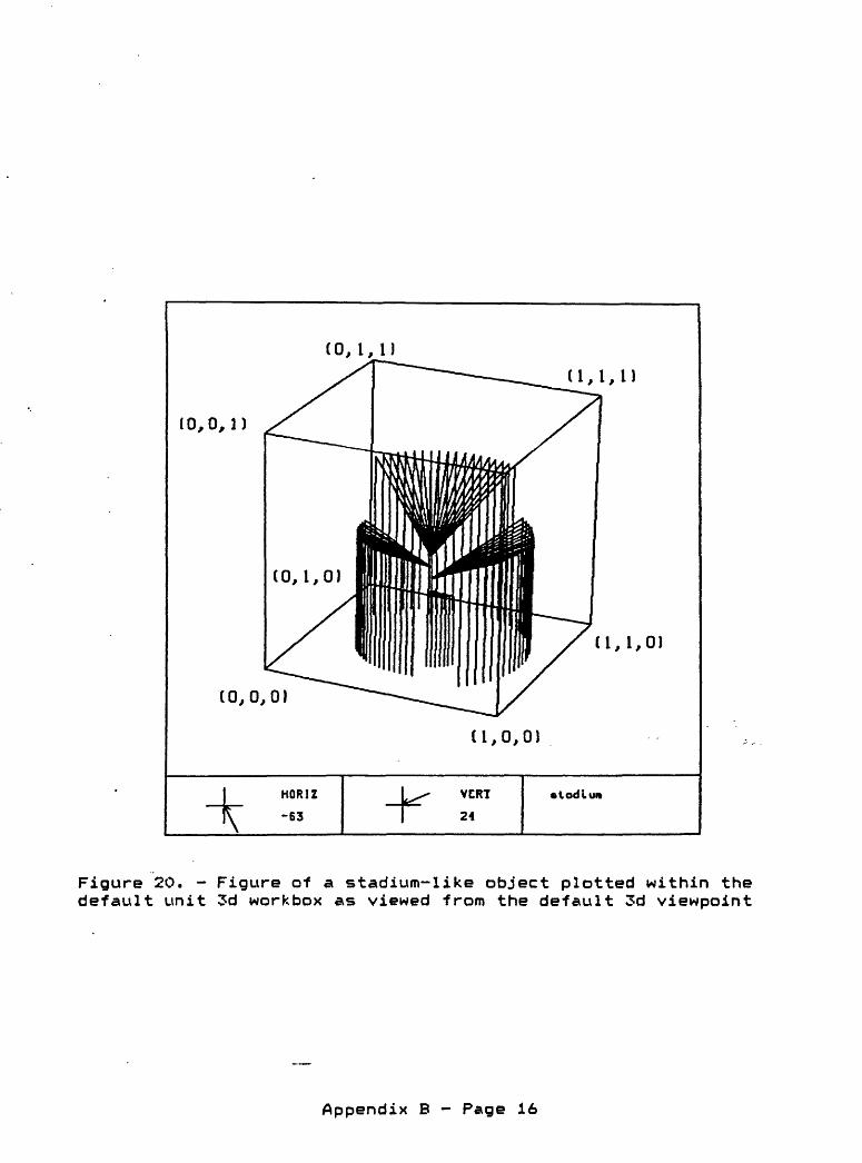
(0,I, 1)
(0,0,0)
(1,1,0)
(1,0,0)
HORIZ -63
-K VERT
24
todliM
Figure 20. - Figure of a stadium-like object plotted within the default unit 3d workbox as viewed from the default 3d viewpoint
Appendix B - Page 16

Figure 21. - Four figures of a stadium-like object plotted within specified-workboxes. The workbox dimensions as specified by the Setwkbox subroutine are A) 1,1,1 B) 2,2,2 C) 1,2,1 and D) 1,1,2
Appendix B - Page 17

I HORIZ
71 -135-K VERT
30
SPlRflL
Figure 22. - 3D spiral drawn using absolute 3d coordinates
Appendix B - Page IB

- 3LX" war I" »«
amnn rune
Figure 23. - Defining the orientation of a plane in 3 dimensions for the Strgrafiti subroutine
HOfttt
amnx
Figure 24. - A simple plot using the grafiti commands
Appendix B - Page 19

B
0
Figure 25. - Reproduction of five figures from Foley and Van Dam [23. A) Figure 8.46, page 307. B) Figure 8.47, page 307. C) Figure 8.47, using code on page 308. D) Figure 8.49, page 309 E) Figure 8.41, page 303
J HORIZXT" -135
I/" tCRT
I 31
90 SPIRAL USING
SCALED PLOTTING
Figure 26. 3D spiral plotted using 3d axis commands and 3d scaled plotting
Appendix B - Page 2O

HORIZ -46
VERT
28
PHflSE
DJRGRftM
Figure 27. Graph using 3d axis and scaled plotting commands
Appendix B - Page 21

APPENDIX C
EXAMPLE PROGRAMS

EXAMPLE1.BAS *************
'program examplel.bas to produce figure 4' $INCLUDE: 'jk2dplt.inc'DECLARE SUB drawex (xp! , ypi , ht!)DECLARE SUB drawrect (1, r, b, t)DECLARE FUNCTION VideoHardware% ()'initialize the plot'use this devno% for screen output
devno% = VideoHardware% 'use this devno% for plot file output ' devno% = JKFIL ' CALL SetFnam(JKFIL, "examplel.plt")
xpage = 5ypage = 5CALL Plots(xpage, ypage, devno%, erret%)CALL drawex(5, 5, .5)
'terminate the plotCALL Plot(0, 0, 999)END
SUB drawex (xp, yp, ht)CALL Plot(0, 0, 3)CALL Plot(xp, 0, 2)CALL Plot(xp, yp, 2)CALL Plot(0, yp, 2)CALL Plot(0, 0, 2)
'construct, locate, and plot the text "EXAMPLE" in the center of the plot
t$ = "EXAMPLE"rot = 0X = .5 * (xp - ht * LEN(t$))y - .5 * (yp - ht)CALL Symbol(x, y, ht, t$, 0)
END SUB
SUB drawrect (1, r, b, t)CALL Plot(l, b, 3)CALL Plot(r, b, 2)CALL Plot(r, t, 2)CALL Plot(l, t, 2)CALL Plot(l, b, 2)
END SUB
Appendix C - Page 1

EXAMPLE2.BAS
'program example2.bas to produce figure 6' $INCLUDE: 'jk2dplt.inc''declarations for subroutines to draw each of the four subareasDECLARE SUB upperleft ()DECLARE SUB lowerleft ()DECLARE SUB lowerright ()DECLARE SUB upperright ()DECLARE FUNCTION VideoHardware% ()'program to demonstrate use of basic plot systemDIM SHARED xpage, ypage'set page size and initialize plot'use this devno% for screen output
devno% = VideoHardware% 'use this devno% for plot file output ' devno% = JKFIL' CALL SetFnam(JKFIL, "example2.pit")
xpage = 10 ypage = 10CALL Plots(xpage, ypage, devno%, erret%) IF NOT erret% THEN
'draw outline and four subareasCALL Plot(0, 0, 3)CALL Plot(xpage, 0, 2)CALL Plot(xpage, ypage, 2)CALL Plot(0, ypage, 2)CALL Plot(0, 0, 2)CALL Plot(xpage / 2, 0, 3)CALL Plot(xpage / 2, ypage, 2)CALL Plot(0, ypage / 2, 3)CALL Plot(xpage, ypage / 2, 2)
'comment call for user information useCALL Comment(24, 1, 78, "UPPER LEFT CORNER")
'move origin to upper left subareaCALL Plot(0, ypage / 2, -3)CALL upperleft
'comment call for user information useCALL Comment(24, 1, 78, "LOWER LEFT CORNER")
'move origin to lower left subareaCALL Plot(0, -ypage / 2, -3) CALL lowerleftCAUL lowerierr
'use comment for informationCALL Comment(24, 1, 78, "LOWER RIGHT CORNER")
'move origin for lower right subareaCALL Plot(xpage / 2, 0, -3)CALL lowerright
'use comment for informationCALL Comment(24, 1, 78, "UPPER RIGHT CORNER")
'move origin for upper right subareaCALL Plot(0, ypage / 2, -3) CALL upperright
Appendix C - Page 2

EXAMPLE2.BAS (continued)
'move origin back to original positionCALL Plot(-xpage / 2, -ypage / 2, -3)
'end plotCALL Plot(0, 0, 999)
ELSEPRINT "open error "; erret%
END IF END
SUB lowerleft DIMxary(lO), yary(10)
CALL Newpen(GRED) 'draw axis lines
CALL Plot(l, 1, 3)CALL Plot(4, 1, 2)CALL Plot(l, 1, 3)CALL Plot(l, 4, 2)
'label axesCALL Symbol(.7, 1.9, .2, "Y-AXIS", 90)CALL Symbol(1.9, .4, .2, "X-AXIS", 0)
'show use of LINE callFOR i = 1 TO 10
xary(i) = (i - 1) / 3 + 1 yary(i) = xary(i)
NEXT iCALL PolyLine(xary()FOR i = 1 TO 10
yary(i) = SQR(xary(i))NEXT iCALL PolyLine(xary(), yary(), 10, 1, 1,CALL PolyLine(yary(), xary(), 10, 1, 0,
END SUB
SUB lowerrightDIM x(3), y(3), d$(3)
CALL Newpen(GGREEN) 'simple annotated point plotting
Y(l) = 4 x(2) = 4 y(2) = 3 x(3) = 2 y(3) = 1 d$(l) = "PT-1" d$(2) = "PT-2" d$(3) = "PT-3" FOR i = 1 TO 3
yary(), 10, 1, -1, 0, .1)
1) 1)
CALL Csymbol(x(i), xp = x(i) + .2 yp = y(i) - .2
y(i), .15, 3, 0, -1)
Appendix C - Page 3

EXAMPLE2.BAS (continued)*************************
CALL Symbol(x(i) + .15, y(i) - .15, .15, d$(i), 0) NEXT i
END SUB
SUB upperleftht = .25txt$ = "Example 2"xp = xpage / 4 - .5 * ht * LEN(txt$)yp = ypage / 4 - .5 * htCALL Symbol(xp, yp, ht, txt$, 0)
'show use of FACTOR callCALL Factor(.5)CALL Symbol(xp, yp, ht, txt$, 0)CALL Factor(1)
END SUB
SUB upperright'set parameters for standard SYMBOL call
CALL Newpen(GLTBLUE) 'show use of angles with SYMBOL call
ht = .15a$ = " EXAMPLE 2"xp = xpage / 4yp = ypage / 4FOR i = 0 TO 7
d = 45 * iCALL Symbol(xp, yp, ht, a$, d)
NEXT i END SUB
Appendix C - Page 4

EXAMPLES.BAS *************
'program examples.bas showing stages of pipeline' $INCLUDE: 'jk2dplt.inc'DECLARE SUB arrowl (xll, yll, x2i, y2! , hi!)DECLARE SUB xsymbol (x, y, ht, txt$, angle)DECLARE SUB Isymbol (x, y, ht, txt$, angle)DECLARE SUB drawoct (x, y, r)DECLARE FUNCTION VideoHardware% ()
'use this devno% for screen outputdevno% = VideoHardware%
'use this devno% for plot file output ' devno% = JKFIL' CALL SetFnam(JKFIL, "examples.pit")
DIM mat(4, 4) sl% = 1WHILE sl% <> 0
CLSa$ = "PIPELINE DEMO PROGRAM" LOCATE 2, 40 - .5 * LEN(a$) PRINT a$ PRINTINPUT "Insert step number (between 1 and 7 : 0 to quit): "; sl% IF Sl% 0 0 THENxpage = 1ypage = 1CALL Plots(xpage, ypage, devno%, tkerr%)IF sl% <> 7 THEN
CALL Plot(0, 0, 3)CALL Plot(xpage, 0, 2)CALL Plot(xpage, ypage, 2)CALL Plot(0, ypage, 2)CALL Plot(0, 0, 2)CALL Plot(xpage / 2, 0, 3)CALL Plot(xpage / 2, ypage, 2)CALL Plot(0, ypage / 2, 3)CALL Plot(xpage, ypage / 2, 2)
END IF IF sl% >= 2 THEN
CALL Eva12dTran(.25, .25, .5, 0, 45, 1, 1, mat())CALL SetTrn2("CTM", mat())
END IF IF sl% >= 3 THEN
a% = SetClip%(»CTM", .75, 1, 0, 1) END IF IF sl% >= 4 THEN
a% = SetWcWin%(.5, 1, 0, .5)a% = SetWcVp%(0, .5, .5, 1)a% = SetClip%(»CTM", .75, 1, 0, 1)
END IF
Appendix C - Page 5

EXAMPLE3.BAS (continued)
IF sl% >= 5 THENCALL Eval2dTran(.25, .75, .5, 0, 45, 1, 1, mat())CALL SetTrn2("WS" / mat())
END IF IF sl% >= 6 THEN
a% = SetClip%("WS", 0, 1, .75, 1) END IF IF sl% >= 7 THEN
a% = SetWsWin%(.5, 1, .5, 1)a% = SetWsVp%(120, 240, 120, 360)a% = SetClip%("WS" / 0, 1, .75, 1)
END IFCALL drawoct(.25, .25, .22) CALL Plot(0, 0, 999)
END IF WEND
END
- XI))
SUB arrowl (xl, yl, x2, y2, hi) IF xl = X2 THEN
IF y2 > yl THENangl = 3.14157 / 2
ELSEangl = 3 * 3.14157
END IF ELSE
angl = ATN((y2 - yl) IF X2 < xl THEN
angl = angl + 3 END IF
END IFrang2 = angl + rang3 = angl - 30 CALL Plot(xl, yl, 3) CALL Plot(x2, y2, 2)CALL Plot(x2 - hi * COS(rang2), y2 - hi * SIN(rang2), CALL Plot(x2, y2, 3)
14157
30 * *
3.14157 / 180 3.14157 / 180
2)
CALL Plot(x2 - hi * COS(rang3), y2 - hi * SIN(rang3), 2)END
SUB
SUB
drawoct (x, y, r) 1 = r / (1 + CALL Plot(x + CALL Plot(x - CALL Plot(X - CALL Plot(x - CALL Plot(x - CALL Plot(x + CALL Plot(x + CALL Plot(x + CALL Plot(x +
1.414)i, y i, y r, y r, y i/ y i, y r, y r, y i, y
r, r, 1, 1, r, r, 1, 1, r,
3) 2) 2) 2) 2) 2) 2) 2) 2)
Appendix C - Page 6

EXAMPLES.BAS (continued) **************
CALL Plot(x - 1, y + r, 3) CALL Plot(x - 1, y - r, 2) CALL Plot(x - 1 / 2, y + r, 3) CALL Plot(x - 1 / 2, y - r, 2) CALL Plot(x, y + r, 3) CALL Plot(x, y - r, 2) CALL Plot(x + 1 / 2, y + r, 3) CALL Plot(x + 1 / 2, y - r, 2) CALL Plot(x +1, y + r, 3) CALL Plot(x + 1, y - r, 2)
END SUB
SUB Isymbol (x, y, ht, txt$, angle)xp = x - ht * (LEN(txt$) + .5)yp = y = .5 * htCALL Symbol(xp, y, ht, txt$, angle)
END SUB
SUB xsymbol (x, y, ht, txt$, angle) xp = x - .5 * ht * LEN(txt$) CALL Symbol(xp, y, ht, txt$, angle)
END SUB
Appendix C - Page 7

EXAMPLE4.BAS *************
'program example4.bas to produce figure 17' $INCLUDE: 'jk2dplt.inc'' $INCLUDE: 'ax2d.inc'DECLARE FUNCTION VideoHardware% ()
dm% = 100DIM xary(dm%), yary(dm%)
'define parabolaxmin = 1E+20ymin = xminxmax = -xminymax = xmaxFOR i% = 1 TO 10
xary(i%) = i% yary(i%) = (5.5 - i%) "2 IF xary(i%) < xmin THEN xmin = xary(i%) IF yary(i%) < ymin THEN ymin = yary(i%) IF xary(i%) > xmax THEN xmax = xary(i%) IF yary(i%) > ymax THEN ymax = yary(i%)
NEXT i% 'use this devno% for screen output
devno% = VideoHardware% 'use this devno% for plot file output ' devno% = JKFIL' CALL SetFnam(JKFIL, "example4.pit") 'draw page outline
xpage = 7: ypage = 7CALL Plots(xpage, ypage, devno%, ierr%)CALL Plot(0, 0, 3)CALL Plot(xpage, 0, 2)CALL Plot(xpage, ypage, 2)CALL Plot(0, ypage, 2)CALL Plot(0, 0, 2)
'draw the axes - left, simple sideCALL ResetAxesCALL Plot(0, 4, -3)CALL SetAxpg(3, 3, "SIMPLE", "X-AXIS", "Y-AXIS", 2, 2)
'autoplot centers the 2x2 inch axis square in the 3x3 page squarea% = autoplt%(3, 3, xmin, xmax, ymin, ymax, errmsg$)
'draw the parabolaCALL spolyline(xary(), yary(), 10, 1, 0, tkiq%, ht)
'draw the axes - right, fancy sideCALL Plot(0, -4, -3)CALL Plot(4, 4, -3)CALL ResetAxesCALL SetAxpg(3, 3, "FANCY", " X-AXIS", "Y-AXIS", 2, 2)
'calculate defaults firsta% = axis2%(3, 3, xmin, xmax, ymin, ymax, -1, errmsg$)CALL xticks(4)CALL yticks(4)CALL grid(2, 2)
Appendix C - Page 8

EXAMPLE4.BAS (continued)c******
'draw the regular axesa% = axis2%(3, 3, xmin, xmax, ymin, ymax, 0, errmsgS)
'draw the parabolaCALL spolyline(xary(), yaryO, 10, 1, 0, tkiq%, ht)
'draw the opposite side axesCALL SetAxisC'Y'', 1, -5, 5, 25, 2, "RIGHT SIDE", -1, 2.5, .5)CALL SetAxisC'X", 1, 0, 2, 12, 2, "", -1, .5, 2.5)CALL Plot(-4, -4, -3)
'example using log type axis for y axisFOR i% = 1 TO 100 yary(i%) = CSNG(i%) / 100 xary(i%) = EXP(-3! * yary(i%)) * SIN(yary(i%) * 8 * 3.14157)
NEXT i%CALL ResetAxesCALL SetAxpg(3, 3, "SIMPLE-LOG", " X-AXIS", "Y-LOGAXIS", 2, 2)CALL SetAxesd, -1, .5, 1, 3, .01, 1, 0)CALL spolyline(xary(>, yaryO, 100, 1, 0, tkiq%, ht)CALL Plot(4, 0, -3)CALL ResetAxesCALL SetAxpg(3, 3, "FANCY-LOG", » X-AXIS", "Y-LOGAXIS", 2, 2)CALL xticks(5)CALL frameCALL SetAxesd, -1, .5, 1, 3, .01, 1, 0)CALL srid(5, 1)CALL spolyline(xary(), yaryO, 100, 1, 0, tkiq%, ht)CALL SetAxisC'Y", 3, .01, 1, 0, 2, "RIGHT SIDE", -1, 2.5, .5)CALL SetAxisC'X", 1, -1, .5, 1, 2, "", -1, .5, 2.5)CALL Plot(-4, 0, -3)CALL Plot(0, 0, 999)END
Appendix C - Page 9
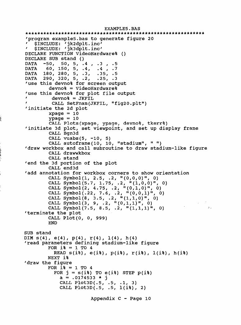
EXAMPLES.BAS *************
'program examples.bas to generate figure 20' $INCLUDE: 'jk2dplt.inc'' $INCLUDE: 'jk3dplt.inc'DECLARE FUNCTION VideoHardware% ()DECLARE SUB stand ()DATA -50, 50, 5, .4 , .3 , .5DATA 60, 150, 5, .4, .4 , .7DATA 180, 280, 5, .3, .35, .5DATA 290, 320, 5, .2, .25, .3'use this devno% for screen output
devno% = VideoHardware% 'use this devno% for plot file output ' devno% = JKFIL' CALL SetFnam(JKFIL, "fig20.plt") 'initiate the 2d plot
xpage =10ypage =10CALL Plots(xpage, ypage, devno%, tkerr%)
'initiate 3d plot, set viewpoint, and set up display frameCALL Bgn3dCALL vuabs(5, -10, 5)CALL autoframe(10, 10, "stadium", " ")
'draw workbox and call subroutine to draw stadium-like figureCALL drawwkboxCALL stand
'end the 3d portion of the plotCALL end3d
'add annotation for workbox corners to show orientationCALL Symbol(1, 2.5, .2, "(0,0,0)", 0)CALL Symbol(5.7, 1.75, .2, "(1,0,0)", 0)CALL Symbol(2, 4.75, .2, "(0,1,0)", 0)CALL Symbol(.22, 7.6, .2, "(0,0,1)", 0)CALL Symbol(8, 3.5, .2, "(1,1,0)", 0)CALL Symbol(3, 9, .2, "(0,1,1)", 0)CALL Symbol(7.5, 8.5, .2, "(1,1,1)", 0)
'terminate the plotCALL Plot(0, 0, 999)END
SUB standDIMS(4), e(4), p(4), r(4), 1(4), h(4) 'read parameters defining stadium-like figure
FOR i% = 1 TO 4READ s(i%), e(i%), p(i%), r(i%), l(i%), h(i%)
NEXT i% 'draw the figure
FOR i% = 1 TO 4FOR j = s(i%) TO e(i%) STEP p(i%)
a = .0174533 * j CALL Plot3D(.5, .5, .1, 3) CALL Plot3D(.5, .5, l(i%), 2)
Appendix C - Page 10

EXAMPLES.BAS (continued)************************
CALL Plot3D(.5 + r(i%) * COS(a), .5 + r(i%) * SIN(a), h(i%), 2) CALL Plot3D(.5 + r(i%) * COS(a), .5 + r(i%) * SIN(a), 0, 2)
NEXT j NEXT i%
END SUB
Appendix C - Page 11

EXAMPLES.BAS *************
'program examples.bas to produce figure 21' $INCLUDE: 'jk2dplt.inc'' $INCLUDE: 'jk3dplt.inc'DECLARE FUNCTION VideoHardware% ()DECLARE SUB stand ()DECLARE SUB frmdrw (xl, xu, yl, yu, bx, by, bz)DIMxl(4), x2(4), yl(4), y2(4) , bx(4), by(4) , bz(4), bs$(4)DIM SHARED s(4), e(4), p(4), r(4), 1(4), h(4)'define the 3d viewports, the workbox sides, and identifying symbolDATA .5, 4.5, 6, 10, 1, 1, 1, "A"DATA 5.5, 9.5, 6, 10, 2, 2, 2, "B"DATA .5, 4.5, 1, 5, 1, 2, 1, "C"DATA 5.5, 9.5, 1, 5, 2, 1, 2, "D"'define the stadium-like figureDATA -50, 50, 10, .4 , .3 , .5DATA 60, 150, 10, .4, .4 , .7DATA 180, 280, 10, .3, .35, .5DATA 290, 320, 10, .2, .25, .3
FOR i% = 1 TO 4 READ x1(i%), x2(i%), y1(i%), y2(i%), bx(i%), by(i%), bz(i%), bs$(i%)
NEXT i%FOR i% = 1 TO 4READ s(i%), e(i%), p(i%), r(i%), l(i%), h(i%)
NEXT i% 'use this devno% for screen output
devno% = VideoHardware% 'use this devno% for plot file output ' devno% = JKFIL' CALL SetFnam(JKFIL, "fig21.plt") 'initiate the 2d plot
xpage = 10ypage = 10.5CALL Plots(xpage, ypage, devno%, tkerr%)CALL Plot(0, 0, 3)CALL Plot(xpage, 0, 2)CALL Plot(xpage, ypage, 2)CALL Plot(0, ypage, 2)CALL Plot(0, 0, 2)
'draw the four viewports, workboxes, and figures withinht = .2FOR i% = 1 TO 4
CALL Symbol(xl(i%), yl(i%) - 2 * ht, ht, bs$(i%), 0) CALL frmdrw(x1(i%), x2(i%), y1(i%), y2(i%), bx(i%), by(i%), bz(i%))
NEXT i% 'terminate the plot
CALL Plot(0, 0, 999)END
Appendix C - Page 12

EXAMPLES.BAS (continued) *******************
SUB frmdrw (xl, xu, yl, yu, bx, by, bz)'subroutine to draw the specified viewport, workbox, and figure
'outline the workboxCALL Plot(xl, yl, 3)CALL Plot(xu, yl, 2)CALL Plot(xu, yu, 2)CALL Plot(xl, yu, 2)CALL Plot(xl, yl, 2)
'begin 3d plotting and set viewpointCALL Bgn3dCALL vuabs(5, -10, 5)
'set the specified 3d viewport and the workboxCALL setvp3d(xl, xu, yl, yu)CALL setwkbox(bx, by, bz)
'draw the workbox and figureCALL drawwkboxCALL stand
'end this portion of the 3d drawingCALL end3d
END SUB
SUB stand'subroutine to draw a stadium-like figure
FOR i% = 1 TO 4FOR j = s(i%) TO e(i%) STEP p(i%)
a = .0174533 * j CALL Plot3D(.5, .5, .1, 3) CALL Plot3D(.5, .5, l(i%), 2)
CALL Plot3D(.5 + r(i%> * COS(a), .5 + r(i%> * SIN(a>, h(i%>, 2) CALL Plot3D(.5 + r(i%> * COS(a), .5 + r(i%) * SIN(a), 0, 2)
NEXT j NEXT i%
END SUB
Appendix C - Page 13

EXAMPLE?.BAS *************
'program example?.bas to produce figure 22' $INCLUDE: 'jk2dplt.inc'' $INCLUDE: 'jk3dplt.inc'DECLARE FUNCTION VideoHardware% ()
npts% = 180 DIM xx(npts%), yy(npts%), zz(npts%)
deg2rad = 3.14159 / 180theta = -90phi = 0rad = 180
'define the spiralFOR i% = 1 TO npts% rth = theta * deg2rad rph = phi * deg2radxx(i%) = rad * COS(rth) * COS(rph) + 150 yy(i%) = rad * COS(rth) * SIN(rph) + 150 zz(i%) = rad * SIN(rth) + 250 theta = theta + 1 phi = phi + 18 rad = rad - 1
NEXT i% 'use this devno% for screen output
devno% = VideoHardware% 'use this devno% for plot file output ' devno% = JKFIL' CALL SetFnam(JKFIL, "fig22.pit") 'initiate 2d plot
xpage = 8ypage =8.5CALL Plots(xpage, ypage, devno%, ier%)
'initiate the 3d plotCALL Bgn3d
'calculate nice viewpoint specification values and set viewpointrad = 5000rth = 30 * deg2radrph = -135 * deg2radxv = rad * COS(rth) * COS(rph) + 3yv = rad * COS(rth) * SIN(rph) + 3zv = rad * SIN(rth) + 5CALL vuabs(xv, yv, zv)
'set the workbox dimensions and make a nice frame for pictureCALL setwkbox(300, 300, 350)CALL autoframe(xpage, ypage, "SPIRAL", "")
'draw the spiralCALL PolyLine3D(xx(), yy(), zz(), npts%, 1, 0, 1, .1)
'draw some lines to help the view orient the pictureCALL Plot3D(150, 150, 0, 3)CALL Plot3D(150, 150, 350, 2)CALL Plot3D(150, 0, 0, 3)CALL Plot3D(150, 300, 0, 2)CALL Plot3D(0, 150, 0, 3)
Appendix C - Page 14

EXAMPLE?.BAS (continued)
CALL Plot3D(300, 150, 0, 2) 'end the 3d portion of the plot
CALL End3d 'terminate the plot
CALL Plot(0, 0, 999)END
Appendix C - Page 15

EXAMPLES.BAS *************
'program examples.bas to produce figure 24' $INCLUDE: 'jk2dplt.inc'' $INCLUDE: 'jkSdplt.inc'DECLARE FUNCTION VideoHardware% ()'use this devno% for screen output
devno% = VideoHardware% 'use this devno% for plot file output ' devno% = JKFIL' CALL Setfnam(JKFIL, "fig24.plt") 'inititate the 2d plot
xpage = 10ypage = 10CALL Plots(xpage, ypage, devno%, tkerr%)
'initiate the 3d plot, set viewpoint, make nice frame, and draw uorkboxCALL BgnSdCALL vuabs(50, -100, 50)CALL autoframe(10, 10, "GRAFITI", "EXAMPLE") CALL drawwkbox
'start the grafiti plottingCALL Strgrafiti(0, 0, 0, 1, 0, 0, 0, 1, 1)
'make 2d dimensions to fill across the whole uorkbox cube, plot outlinenewy = 1.414newx = 1ht = newy / 15CALL Plot(0, 0, 3)CALL Plot(newx, 0, 2)CALL Plot(newx, newy, 2)CALL Plot(0, newy, 2)CALL Plot(0, 0, 2)
'plot four 2d lines on plane in 3 dimensionsa$ = "A"a = .5 * (1 - LEN(a$) * ht)CALL Symbol(a, 12 * ht, ht, a$, 0)a$ = "SIMPLE"a = .5 * (1 - LEN(a$) * ht)CALL Symbol(a, 9 * ht, ht, a$, 0)a$ = "GRAFITI"a = .5 * (1 - LEN(a$) * ht)dx = .5 * (1 - LEN(a$) * ht - 2 * ht)CALL Symbol(a, 6 * ht, ht, a$, 0)a$ = "CALL"a = .5 * (1 - LEN(a$) * ht)CALL Symbol(a, 3 * ht, ht, a$, 0)
'draw an inner border on the planeCALL Plot(dx, ht, 3)CALL Plot(l - dx, ht, 2)CALL Plot(l - dx, 1.414 - ht, 2)CALL Plot(dx, 1.414 - ht, 2)CALL Plot(dx, ht, 2)
'end grafiti plottingCALL Endgrafiti
Appendix C - Page 16

'end 3d plottingCALL End3d
'terminate the plotCALL Plot(0, 0, 999)END
Appendix C - Page 17

EXAMPLES.BAS *************
'program examples.bas to produce figure 25' $INCLUDE: 'jk2dplt.inc'' $INCLUDE: ' jk3dplt.inc'DECLARE SUB house ()DECLARE SUB windrw (a$)DECLARE FUNCTION VideoHardware% ()'use this devno% for screen output
devno% = VideoHardware% 'use this devno% for plot file output ' devno% = JKFIL' CALL SetFnam(JKFIL, "fig25.plt") 'initiate the 2d plot and draw page outline
xpage = 10ypage = 7CALL Plots(xpage, ypage, devno%, tkerr%)CALL Plot(0, 0, 3)CALL Plot(xpage, 0, 2)CALL Plot(xpage, ypage, 2)CALL Plot(0, ypage, 2)CALL Plot(0, 0, 2)
'Foley and Van Dam, pg 307, fig 8.46 'set the 2d world coordinate viewport, draw and identify viewport
a% = SetWcVp%(l, 3, 4, 6)CALL windrw("A")
'begin 3d plottingCALL Bgn3d
'set viewing parametersCALL setcop(8, 6, 84)CALL setvrp(0, 0, 0)CALL setvpn(0, 0, -1)CALL setvup(0, 1, 0)CALL setuvwin(-50, 50, -50, 50, -100, 100)CALL setvp3d(l, 3, 4, 6)
'cause the plot system to calculate required projection matricesCALL sc!3d2d
'draw the houseCALL house
'end this part of the 3d drawingCALL end3d
'Foley and Van Dam, pg 307, fig 8.47a% = SetWcVp%(4, 6, 4, 6)CALL windrw("B")CALL Bgn3dCALL setvrp(0, 0, 54)CALL setcop(8, 6, 30)CALL setvpn(0, 0, -1)CALL setvup(0, 1, 0)CALL setuvwin(-l, 17, -1, 17, -100, 100)CALL setvp3d(4, 6, 4, 6)CALL sc!3d2dCALL house
Appendix C - Page 18

EXAMPLES.BAS (continued)k*
CALL end3d 'Foley and Van Dam, pg 308, fig 8.47
a% = SetWcVp%(7, 9, 4, 6)CALL windrw("C")CALL Bgn3dCALL setvrp(8, 6, 54)CALL setcop(0, 0, 30)CALL setvpn(0, 0, -1)CALL setvup(0, 1, 0)CALL setuvwin(-9, 9, -7, 11, -100, 100)CALL setvp3d(7, 9, 4, 6)CALL sc!3d2dCALL houseCALL end3d
'Foley and Van Dam, pg 309, fig 8.49a% = SetWcVp%(2.5, 4.5, 1, 3)CALL windrw("D")CALL Bgn3dCALL setvrp(16, 0, 54)CALL setcop(20, 25, 20)CALL setvpn(0, 0, -1)CALL setvup(0, 1, 0)CALL setuvwin(-20, 20, -5, 35, -1000, 1000)CALL setvp3d(2.5, 4.5, 1, 3)CALL sc!3d2dCALL houseCALL end3d
'Foley and Van Dam, pg 311, fig 8.41a% = SetWcVp%(5.5, 7.5, 1, 3)CALL windrw("E")CALL Bgn3dCALL setvrp(16, 0, 54)CALL setcop(20, 25, 20)CALL setvpn(-l, 0, -1)CALL setvup(0, 1, 0)CALL setuvwin(-12, 13, -2, 23, -100, 100)CALL setvp3d(5.5, 7.5, 1, 3)CALL sc!3d2dCALL houseCALL end3d
'terminate the plotCALL Plot(0, 0, 999)END
SUB house'front face of house at z=30
CALL Plot3D(0, 0, 30, 3)CALL Plot3D(16, 0, 30, 2)CALL Plot3D(16, 10, 30, 2)CALL Plot3D(8, 16, 30, 2)CALL Plot3D(0, 10, 30, 2)
Appendix C - Page 19

EXAMPLES.BAS (continued) ************
CALL Plot3D(0, 0, 30, 2) 'back face at z=54
CALL Plot3D(0, 0, 54, 3)CALL Plot3D(16, 0, 54, 2)CALL Plot3D(16, 10, 54, 2)CALL Plot3D(8, 16, 54, 2)CALL Plot3D(0, 10, 54, 2)CALL Plot3D(0, 0, 54, 2)
'connect front and backCALL Plot3D(0, 0, 30, 3)CALL Plot3D(0, 0, 54, 2)CALL Plot3D(16, 0, 30, 3)CALL Plot3D(16, 0, 54, 2)CALL Plot3D(16, 10, 30, 3)CALL Plot3D(16, 10, 54, 2)CALL Plot3D(8, 16, 30, 3)CALL Plot3D(8, 16, 54, 2)CALL Plot3D(0, 10, 30, 3)CALL Plot3D(0, 10, 54, 2)
END SUB
SUB windrw (a$)a% = SetWcWin%(0, 1, 0, 1)CALL Plot(0, 0, 3)CALL Plot(l, 0, 2)CALL Plot(l, 1, 2)CALL Plot(0, 1, 2)CALL Plot(0, 0, 2)a% = ResetClip%("CTM")CALL Symbol(0, -.2, .1, a$, 0)
END SUB
Appendix C - Page 20

EXAMPL10.BAS *************
'program exampllO.bas to produce figure 26' $INCLUDE: 'jk2dplt.inc'' $INCLUDE: 'ax2d.inc'' $INCLUDE: 'jk3dplt.inc'' $INCLUDE: 'ax3d.inc'DECLARE FUNCTION VideoHardware% ()'extend the stack for big program
CLEAR , , 2000DIM prmx AS AxprmT, prmy AS AxprmT, prmz AS AxprmT 'use this devno% for screen output
devno% = VideoHardware% 'use this devno% for plot file output ' devno% = JKFIL' CALL SetFnam(JKFIL, "fig26.plt") 'define the 3d spiral - this time without including a translation
npts% = 180 DIM xx(npts%), yy(npts%), zz(npts%)
deg2rad = 3.14159 / 180npts% =180theta = -90phi = 0rad = 180FOR i% = 1 TO npts%
rth = theta * deg2rad rph = phi * deg2rad xx(i%) = rad * COS(rth) * COS(rph) yy(i%) = rad * COS(rth) * SIN(rph) zz(i%) = rad * SIN(rth) theta = theta + 1 phi = phi + 18 rad = rad - 1
NEXT i% 'initialize the 2d plot system
xpage =8ypage = 8.5 ;,CALL Plots(xpage, ypage, devno%, ier%)
'plot the page outline in 2dCALL Plot(0, 0, 3)CALL Plot(xpage, 0, 2)CALL Plot(xpage, ypage, 2)CALL Plot(0, ypage, 2)CALL Plot(0, 0, 2)
'initialize the 3d plot systemCALL Bgn3d
'show the calculation of the viewpoint locationa = 30b = -135c = 500rad = crth = a * deg2radrph = b * deg2rad
Appendix C - Page 21

EXAMPL10.BAS (continued) ***********************
xv = rad * COS(rth) * COS(rph) + 3yv = rad * COS(rth) * SIN(rph) + 3zv = rad * SIN(rth) + 5CALL vuabs(xv, yv, zv)
' include a nice framettll$ = "3D SPIRAL USING"tt!2$ = "SCALED PLOTTING"CALL autoframe(xpage, ypage, ttll$, tt!2$)
'set the workbox dimensions using the SetAxpg3d commandCALL SetAxpg3d("", 6, "", 6, "", 7)
'set the 3d axis system so that the spiral with be drawn in 'the center of the workbox
CALL setaxes3d(l, -150, 50, 150, 1, -150, 50, 150, 1, 250, 50, 100, 0) 'draw the spiral
CALL spoly3d(xx(), yy(), zz(), npts%, l, 0, 1, .1) 'add some lines parallel to the axes to help visualation
CALL splot3d(0, 0, -250, 3)CALL splot3d(0, 0, 100, 2)CALL splot3d(0, -150, -250, 3)CALL splot3d(0, 150, -250, 2)CALL splot3d(-150, 0, -250, 3)CALL splot3d(150, 0, -250, 2)
'terminate the 3d portion of the plotCALL end3d
'terminate the plotCALL Plot(0, 0, 999)END
Appendix C - Page 22

EXAMPL11.BAS *************
'program examplll.bas to produce figure 27' $INCLUDE: 'jk2dplt.inc'' $INCLUDE: 'jk3dplt.inc'' $INCLUDE: 'ax2d.inc'' $INCLUDE: 'Ax3d.inc'DECLARE FUNCTION VideoHardware% ()DIM prmx AS AxprmT, prmy AS AxprmT, prmz AS AxprmTDIMx(lO), y(10), z(10), xx(10), zO(10)'set extra stack space for big program
CLEAR , , 2000 'use this devno% for screen output
devno% = VideoHardware% 'use this devno% for plot file output ' devno% = JKFIL' CALL SetFnam(JKFIL, "fig27.pit") 'define the 3d curve
npts% = 10 FOR i% = 1 TO 10
zs = 1.4 * CSNG(i%) z(i%) = zsys = zs * zs / 65.33 y(i%) = ysxs = 1.2 + .2 * ys * ys x(i%) = 10 A xs xx (i%) = xs zO(i%) = 0
NEXT i%'set page size and initialize the 2d plot system
xpage = 6.5 ypage = 8CALL Plots(xpage, ypage, devno%, ier%)
'initialize the 3d plot system, specify viewing parameters, and frame CALL Bgn3dCALL vuabs(30, -31, 23)CALL autoframe(xpage, ypage, "PHASE", "DIAGRAM")
'set the 3d axis page (and thus workbox dimensions) and labelsCALL SetAxpg3d("", 7, "PHASE", 3, "AMPLITUDE", 3)
'specify that only the Y and Z axis annotation is to be drawnCALL nodraw3d("ON", "OFF", "OFF")
'change from default height to the labels can be readCALL SetAxht3(.13, .13, .13)
'specify the axis types and limits and draw axes 'note that because the X axis is not drawn the axes are disconnected
CALL setaxes3d(3, 10, 3.5, 1000, 1, 0, 1, 3, 1, 0, 3, 15, 0) 'draw the main 3d curve
CALL spoly3d(x(), y(), zO, 10, 1, 1, 1, .1)'draw lines parallel to the z and x axes to each of the line nodes 'to help with 3d visualization
FOR i% = 1 TO npts%CALL splot3d(x(i%), y(i%), 0, 3) CALL splot3d(x(i%), y(i%), z(i%), 2)
Appendix C - Page 23

EXAMPL11.BAS (continued) ***********************
CALL splot3d(10, y(i%), z(i%), 2)NEXT i%
'add supplementary annotation for the x axis using grafiti and '2d axis commands in the grafiti plane defined by the equation Z=0 'the grafiti XY plane is thus the XY 3d plane also
CALL strgrafiti(0, 0, 0, 1, 0, 0, 0, 1, 0)CALL ResetAxesCALL SetAxht2(.13, .13)
'specify that only the X axis is to be drawnCALL nodraw("OFF", "ON")CALL SetAxis("X", 3, 10, 3.5, 1000, 7, "FREQUENCY", 1, 0,
0)CALL SetAxis("Y", 1, 0, 1, 3, 3, "", 1, 0, 0)CALL frame
'draw the 2d trace of the 3d curve in the plane Z=10CALL spolyline(x(), y(), 10, 1, 1, 2, .15)
'add grid to the plane Z=0CALL nodraw("OFF", "OFF")CALL grid(l, 2)CALL endgrafiti
'add supplementary annotation for the x axis using grafiti and '2d axis commands in the grafiti plane defined by the equation Y=0 'the grafiti XY plane is now the 3d YZ plane
CALL strgrafiti(0, 0, 0, 0, 1, 0, 0, 0, 1) 'draw only the grafiti X axis (the 3d Y axis)
CALL nodraw("OFF", "ON")CALL SetAxht2(.08, .08)CALL SetAxis("X", 1, 0, .5, 3, 3, "PHASE", -1, 0, 3)CALL SetAxis("Y", 1, 0, 3, 15, 3, "", 1, 0, 0)CALL frame
'specify that both axes are to be griddedCALL nodraw("OFF", "OFF")CALL grid(l, 1)
'draw the trace of the 3d curve on the plane YZ (Log X = 1)CALL spolyline(y(), z(), 10, 1, 1, 3, .15)
'terminate the plotCALL endgrafitiCALL end3dCALL Plot(0, 0, 999)END
Appendix C - Page 24

APPENDIX D
EXAMPLE INTERMEDIATE PLOT FILES

EXAMPLE 1 PLOT FILE ***********
PLOTS, 5 , 5PLOT, 0,0,3PLOT, 5,0,2PLOT, 5,5,2PLOT, 0,5,2PLOT, 0,0,2SSYMBOL, .75 , 2.25 , .5 , 0 ,EXAMPLEPLOT, 0,0, 999
Appendix D - 1

EXAMPLE 2 PLOT FILE *********
PLOTS, 10 , 10PLOT, 0,0,3PLOT, 10 , 0 , 2PLOT, 10 , 10 , 2PLOT, 0 , 10 , 2PLOT, 0,0,2PLOT, 5,0,3PLOT, 5 , 10 , 2PLOT, 0,5,3PLOT, 10 , 5 , 2NCOMHENT, 24 , 1 , 78 ,UPPER LEFT CORNERPLOT, 0 , 5 ,-3SSYMBOL, 1.375 , 2.375 , .25 , 0 ,Example 2FACTOR, .5SSYMBOL, 1.375 , 2.375 , .25 , 0 ,Example 2FACTOR, 1NCOMHENT, 24 , 1 , 78 ,LOWER LEFT CORNERPLOT, 0 ,-5 ,-3NEWPEN, 13PLOT, 1,1,3PLOT, 4,1,2PLOT, 1,1,3PLOT, 1,4,2SSYMBOL, .7 , 1.9 , .2 , 90 ,Y-AXISSSYMBOL, 1.9 , .4 , .2 , 0 ,X-AXISPOLYLINE, 10 , 1 ,-1 , 0 , .11/11.333333,1.3333331.666667,1.6666672,22.333333,2.3333332.666667,2.6666673,33.333333,3.3333333.666667,3.6666674,4POLYLINE, 10 , 1 , 1 , 1 , .11/11.333333,1.1547011.666667,1.2909952,1.4142142.333333,1.5275252.666667,1.6329933,1.7320513.333333,1.8257423.666667,1.9148544/2POLYLINE, 10 , 1 , 0 , 2 , .11/1 1.154701,1.333333
Appendix D - 2

EXAMPLE 2 PLOT FILE (continued)
1.290995,1.6666671.414214,21.527525,2.3333331.632993,2.6666671.732051,31.825742,3.3333331.914854,3.6666672/4NCOMMENT, 24 , 1 ,PLOT, 5 , 0 ,-3NEWPEN, 7CSYMBOL, 1 , 4 , .15 ,SSYMBOL, 1.15 , 3.85 ,CSYMBOL, 4 , 3 , .15 ,SSYMBOL, 4.15 , 2.85 ,CSYMBOL, 2 , 1 , .15 ,SSYMBOL, 2.15 , .85 ,NCOMMENT, 24 , 1 , 78PLOT, 0 , 5 ,-3NEWPEN, 6SSYMBOL, 2.5SSYMBOL, 2.5SSYMBOL, 2.5SSYMBOL, 2.5SSYMBOL, 2.5SSYMBOL, 2.5SSYMBOL, 2.5SSYMBOL, 2.5PLOT,-5 ,-5 ,PLOT, 0 , 0 4
78 ,LOWER RIGHT CORNER
3 , 0 ,-1.15 , 0 ,PT-13 , 0 ,-1.15 , 0 ,PT-23 , 0 ,-1 .15 , 0 ,PT-3 ,UPPER RIGHT CORNER
EXAMPLE 2 EXAMPLE 2 EXAMPLE 2 EXAMPLE 2 EXAMPLE 2 EXAMPLE 2 EXAMPLE 2 EXAMPLE 2
/ 2.5 ,/ 2.5 ,/ 2.5 ,/ 2.5 ,/ 2.5 ,/ 2.5 ,, 2.5 ,/ 2.5 ,-3
999
- .15 t, .15 t
. 15 ,. .15 ,
. 15 t
.15 ,
. 15 t
.15 ,
r 0 ,
r 45 ,
r 90 ,
r 135 ,
r 180 ,
r 225 ,
r 270 ,
r 315 ,
Appendix D - 3

EXAMPLE 4 PLOT FILE ***********
PLOTS f 7 f 7PLOT, 0,0,3PLOT, 7,0,2PLOT, 7,7,2PLOT, 0,7,2PLOT, 0,0,2RESETAXESPLOT, 0 , 4 ,-3SETAXP6, 3,3,2,2SIMPLEX-AXISY-AXISAUTOPLT, 3 , 3 , 1 , 10 , .25 , 20.25SPOLYLINE, 10 , 1 , 0 , 0 , 01,20.252,12.253,6.254,2.255,.256,.257,2.258,6.259,12.2510,20.25PLOT, 0 ,-4 ,-3PLOT, 4 , 4 ,-3RESETAXESSETAXP6, 3,3,2,2FANCY
X-AXIS Y-AXISAXIS2, 3 , 3 , 1 , 10 , .25 , 20.25 ,-1 XTICKS, 4 YTICKS, 4 GRID, 2,2AXIS2, 3 , 3 , 1 , 10 , .25 ,20.25 , 0 SPOLYLINE, 10 , 1 , 0 , 0 , 0 1,20.25 2,12.25 3,6.25 4,2.25 5,.25 6,.25 7,2.25 8,6.25 9,12.25 10,20.25SETAXIS,Y, 1 ,-5 , 5 , 25 , 2 ,-1 , 2.5 , .5 ,RIGHT SIDE SETAXIS,X, 1,0,2,12,2,-!, .5,2.5, PLOT,-4 ,-4 ,-3 RESETAXES
Appendix D - 4

EXAMPLE 4 PLOT FILE (continued)-*******SETAXPG, 3,3,2,2SIMPLE-LOGX-AXIS
Y-LOGAXISSETAXES, 1 ,-1 , .5 , 1 , 3 , .01 SPOLYLINE, 100 ,1,0,0,0 .2413383,.01 .4536956,.02 .6256253,.03 .7488483,.04 .8185796,.05 .8336214,.06 .7962285,.07 .711767,.08 .5882019,.09 .4354528,.1 .2646668,.11 8.745702E-02,.12-8.484181E-02, .13-.2418596,.14-.3747746,.15-.4767694,.16-.5433368,.17-.5724226,.18-.5644107,.19-.521957,.2-.449693,.21-.353824,.22-.2416544,.23-.1210708,.24-2.131539E-05,.25 .1139799,.26 .2142932,.27 .2955103,.28 .3537207,.29 .386664,.3 .3937738,.31 .376115,.32 .3362221,.33 .2778573,.34 .2057061,.35 .1250339,.36 4.132653E-02,.37-4.006219E-02,.38-.1142334,.39-.1770199,.4-.2252015,.41-.2566487,.42-.270391,.43-.2666095,.44-.2465587,.45
Appendix D - 5

-*************-.212426,.46-.1671427,.47-.1141588,.48-5.719984E-02,.49-2.013736E-05,.5 5.383093E-02,.51 .1012164,.52 .1395823,.53 .1670811,.54 .1826444,.55 .186005,.56 .1776656,.57 .1588234,.58 .1312555,.59 .0971746,.6 5.906859E-02,.61 1.952824E-02,.62-1.891728E-02,.63-5.395387E-02,.64-8.361311E-02,.65-.1063737,.66-.1212297,.67-.1277225,.68-.1259378,.69-.1164678,.7-.1003458,.71-.0789564..72
EXAMPLE 4 PLOT FILE (continued)
-.1003458,.71-.0789564,.72-5.392922E-02,.73-2.702404E-02,.74-1.426832E-05,.75 2.542346E-02,.76 4.780738E-02,.77 6.593093E-02,.78 7.892124E-02,.79 8.627384E-02,.8 .0878623,.81 8.392403E-02,.82 7.502446E-02,.83 6.200297E-02,.84 4.590493E-02,.85 2.790521E-02,.86 9.227777E-03,.87-8.932694E-03,.88-.0254831,.89-3.949358E-02,.9-.0502455,.91-5.726362E-02,.92-6.033134E-02,.93-5.948896E-02,.94-5.501629E-02,.95-4.740136E-02,.96
Appendix D - 6

EXAMPLE 4 PLOT FILE (continued)r!
-3.729815E-02,.97-2.547645E-02,.98-1.276749E-02,.99-8.986503E-06,!PLOT, 4 , 0 ,-3RESETAXESSETAXP6, 3,3,2,2FANCY-LOG
X-AXIS Y-LO6AXIS XTICKS, 5 FRAMESETAXES, 1 ,-1 , .5 , 1 , 3 , .01 , 1 , 0 GRID, 5 , 1SPOLYLINE, 100 ,1,0,0,0 .2413383,.01 .4536956,.02 .6256253,.03 .7488483,.04 .8185796,.05 .8336214,.06 .7962285,.07 .711767,.08 .5882019,.09 .4354528,.1 .2646668,.11 8.745702E-02,.12-8.484181E-02,.13-.2418596,.14-.3747746,.15-.4767694,.16-.5433368,.17-.5724226,.18-.5644107,.19-.521957,.2-.449693,.21-.353824,.22-.2416544,.23-.1210708,.24-2.131539E-05,.25 .1139799,.26 .2142932,.27 .2955103,.28 .3537207,.29 .386664,.3 .3937738,.31 .376115,.32 .3362221,.33 .2778573,.34 .2057061,.35 .1250339,.36
Appendix D - 7

-**************** 4.132653E-02,.37-4.006219E-02,.38-.1142334,.39-.1770199,.4-.2252015,.41-.2566487,.42-.270391,.43-.2666095,.44-.2465587,.45-.212426,.46-.1671427,.47-.1141588,.48-5.719984E-02,.49-2.013736E-05,.5 5.383093E-02,.51 .1012164,.52 .1395823,.53 .1670811,.54 .1826444,.55 .186005,.56 .1776656,.57 .1588234,.58 .1312555,.59 .0971746,.6 5.906859E-02,.61 1.952824E-02,.62-1.891728E-02,.63-5.395387E-02,.64-8.361311E-02,.65-.1063737,.66-.1212297,.67-.1277225,.68-.1259378,.69-.1164678,.7-.1003458,.71-.0789564,.72-5.392922E-02,.73-2.702404E-02,.74-1.426832E-05,.75 2.542346E-02,.76 4.780738E-02,.77 6.593093E-02,.78 7.892124E-02,.79 8.627384E-02,.8 .0878623,.81 8.392403E-02,.82 7.502446E-02,.83 6.200297E-02,.84 4.590493E-02,.85 2.790521E-02,.86 9.227777E-03,.87
EXAMPLE 4 PLOT FILE (continued)
Appendix D - 8

EXAMPLE 4 PLOT FILE (continued)M
-8.932694E-03,.88-.0254831,.89-3.949358E-02,.9-.0502455,.91-5.726362E-02,.92-6.033134E-02,.93-5.948896E-02,.94-5.501629E-02,.95-4.740136E-02,.96-3.729815E-02,.97-2.547645E-02,.98-1.276749E-02,.99-8.986503E-06,!SETAXIS,Y, 3,.01,1,0,2,-1,2.5,.5 ,RIGHT SIDESETAXIS,X, 1,-1, .5,1,2,-!, .5,2.5,PLOT,-4 , 0 ,-3PLOT, 0,0, 999
Appendix D - 9

APPENDIX E
JKPLOT FUNCTIONS AND SUBROUTINES (organized by module)

LIST OF SUBROUTINES AND FUNCTIONS ORGANIZED BY CODE MODULE (Long lines are continued onto the next line with indentation)
SUBROUTINES AND FUNCTIONS IN THE JK2DPLT.BAS MODULE
"CalComp-like" entry points SUB Plots (x, y, devno%, tkerr%) ........................... 9SUB Plot (x!, y!, p%) ...................................... 10SUB PolyLine (xary(), yary(), npts%, inc%, lintyp%,
tkiq%, ht) ............................................ 11SUB Symbol (x! , y!, ht!, txt$, angle!) ..................... 10SUB Csymbol (x!, y!, ht!, q%, angle!, icode%) .............. 11SUB Number (x, y, ht, fpn, angle, ndec%) ................... 11SUB Factor (rfact) ......................................... 13SUB Newpen (spen%) ......................................... 12SUB Comment (row%, col%, llen%, txt$) ...................... 13
pipe manipulation entry points FUNCTION ResetClip% (wch$) ................................. 26FUNCTION SetClip% (wch$, 1, r, b, t) ....................... 26
work station entry points SUB SetFnam (wch%, nam$) ................................... 13FUNCTION SetWsWin% (1!, r!, b!, t!) ........................ 25FUNCTION SetWsVp% (1!, r!, b!, t!) ......................... 25
world coordinate entry points FUNCTION SetWcWin% (1!, r!, b!, t!) ........................ 25FUNCTION SetWcVp% (1!, r!, b!, t!) ......................... 25
transformation entry points SUB AcmTrn2 (wch$, mat()) .................................. 26SUB SetTrn2 (wch$, mat()) .................................. 26SUB Eval2dTran (fx!, fy!, tx!, ty!, rotdeg!, sx!,
sy!, mat!()) .......................................... 26font manipulation entry points
SUB newfont (f%) ........................................... 11SUB newcfont (f%) .......................................... 11
SUBROUTINES AND FUNCTIONS IN THE AX2D.BAS MODULE
FUNCTION autoplt% (xpage, ypage, xmin, xmax, ymin,ymax, errmsg$) ........................................ 36
FUNCTION axis2% (xpage, ypage, xmin, xmax, ymin, ymax,calconly%, errmsg$) ................................... 36
SUB eqplt (ind$) ........................................... 36SUB frame () ............................................... 37SUB grid (xgrd%, ygrd%) .................................... 37SUB nodraw (x$, y$) ........................................ 38SUB noend (x$, y$) ......................................... 38SUB nofrst (x$, y$) ........................................ 38SUB nolab (x$, y$) ......................................... 38SUB nolast (x$, y$) ........................................ 38SUB nonum (x$, y$) ......................................... 38SUB ResetAxes () ........................................... 37SUB scsymbol (x, y, ht, tkiq%, angle, icode%) .............. 39
Appendix E - Page 1

SUBROUTINES AND FUNCTIONS IN THE AX3D.BAS MODULE (continued)
SUB SetAxht3 (xht, yht, zht) ............................... 52SUB SetAxpg3d (x3l$, x3ax, y3l$, y3ax, z3l$, z3ax) ......... 51SUB splot3d (x, y, z, p%) .................................. 52SUB spoly3d (xary(), yary(), zary(), npts%, inc%, lintyp%,
tkiq%, ht) ............................................ 52
Appendix E - Page 3

APPENDIX F
JKPLOT FUNCTIONS AND SUBROUTINES
(organized alphabetically)

LIST OF SUBROUTINES AND FUNCTIONS ORGANIZED ALPHABETICALLY (Long lines are continued onto the next line with indentation)
SUB AcmTrn2 (wch$, mat()) .................................. 26SUB autoframe (xpage, ypage, ttll$, tt!2$) ................. 44FUNCTION autoplt% (xpage, ypage, xmin, xmax, ymin,
ymax, errmsg$) ........................................ 36FUNCTION axis2% (xpage, ypage, xmin, xmax, ymin, ymax,
calconly%, errmsg$) ................................... 36SUB Bgn3d () ............................................... 43SUB Comment (row%, col%, llen%, txt$) ...................... 13SUB Csymbol (x!, yl, htl, tkiq%, anglel, icode%) ........... 11SUB Csymbol3D (x!, yl, zl, htl, q%, anglel, icode%) ........ 45SUB drawwkbox () ........................................... 42SUB end3d () ............................................... 43SUB endgrafiti () .......................................... 46SUB eqplt (ind$) ........................................... 36SUB Eval2dTran (fxl, fyl, txl, tyl, rotdegl, sxl,
syl, matl()) .......................................... 26SUB Factor (rfact) ......................................... 13SUB frame () ............................................... 37SUB grid (xgrd%, ygrd%) .................................... 37SUB newcfont (f%) .......................................... 11SUB newfont (f%) ........................................... 11SUB Newpen (spen%) ......................................... 12SUB nodraw (x$, y$) ........................................ 38SUB nodraw3d (x$, y$, z$) .................................. 52SUB noend (x$, y$) ......................................... 38SUB nofrst (x$, y$) ........................................ 38SUB nolab (x$, y$) ......................................... 38SUB nolast (x$, y$) ........................................ 38SUB nonum (x$, y$) ......................................... 38SUB Number (x, y, ht, fpn, angle, ndec%) ................... 11SUB Plot (xl, yl, p%) ...................................... 10SUB Plot3D (xl, yl, zl, p%) ................................ 45SUB Plots (x, y, devno%, tkerr%) ........................... 9SUB PolyLine (xary(), yary(), npts%, inc%, lintyp%, -
tkiq%, ht) ............................................ 11SUB PolyLine3D (x3l(), y3l(), z3i(), npts%, inc%, lintyp%,
tkiq%, htl) ........................................... 45SUB ResetAxes () ........................................... 37FUNCTION ResetClip% (wch$) ................................. 26SUB Scl3d2d () ............................................. 48SUB scsymbol (x, y, ht, tkiq%, angle, icode%) .............. 39SUB SetAxes (xtyp, xorig, xstep, xend, ytyp, yorig,
ystep, yend)........................................... 36SUB setaxes3d (xt, xs, xp, xe, yt, ys, yp, ye, zt, zs,
zp, ze, nodraw3%) ..................................... 37SUB SetAxht2 (xht1, yht1) .................................. 37SUB SetAxht3 (xht, yht, zht) ............................... 51SUB SetAxis (wch$, atyp, aorig, astep, aend, alen,
alab$, aside%, xpos, ypos) ............................ 35SUB SetAxpg (xpage, ypage, tit$, xlab$, ylab$, xlen, ylen) . 37
Appendix F - Page 1

APPENDIX 6
JKPLOT FUNCTIONS AND SUBROUTINES WITH FILE OUTPUT FORMORGANIZED BY MODULE

LIST OF SUBROUTINES AND FUNCTIONS FOR JKPLOT FILE OUTPUTORGANIZED BY CODE MODULE
(Long lines are continued onto the next line with indentation)
SUBROUTINES AND FUNCTIONS IN THE JK2DPLT.BAS MODULE ******************************************************
*****»CalComp-like" entry points*****
SUB Plots (x, y, devno%, tkerr%) PLOTS, x, y
SUB Plot (x!, y!, p%) PLOT, x, y, p%
SUB PolyLine (xary(), yary(), n%, inc%, typ%, q%, ht) POLYLINE, n%, inc%, typ%, q%, ht(Then n% lines are written, each containing an xary and a yary element, seperated by a comma.)
SUB Symbol (x!, y!, ht!, txt$, angle!) SSYMBOL, x, y, ht, angle, txt$
SUB Csymbol (x!, y!, ht!, q%, a, i%) CSYMBOL, x, y, ht, q%, a, i%
SUB Number (x, y, ht, fpn, a, d%) NUMBER, x, y, ht, fpn, a, d%
SUB Factor (rfact) FACTOR, rfact
SUB Newpen (spen%) NEWPEN, spen%
SUB Comment (row%, col%, llen%, txt$) NCOMMENT, row%, col%, llen%, txt$
*****pipe manipulation entry points*****
FUNCTION ResetClip% (wch$) RESETCLIP, wch$
FUNCTION SetClip% (wch$, 1, r, b, t) SETCLIP, wch$, 1, r, b, t
*****work station entry points*****
SUB SetFnam (wch%, nam$)(This subroutine is actually executed within the JKFSEP.bassubroutine; nothing is written to the output file.)
Appendix G - Page 1

LIST OF SUBROUTINES AND FUNCTIONS FOR JKPLOT FILE OUTPUTORGANIZED BY CODE MODULE
continued (Long lines are continued onto the next line with indentation)
FUNCTION SetWsWin% (1!, r!, b!, t!) SETWSWIN, 1, r, b, t
FUNCTION SetWsVp% (1!, r!, b!, t!) SETWSVP, I, I, b, t
*****vorld coordinate entry points*****
FUNCTION SetWcWin% (1!, r!, b!, t!) SETWCWIN, 1, r, b, t
FUNCTION SetWcVp% (1!, r!, b!, t!) SETWCVP, 1, r, b, t
*****transformation entry points*****
SUB AcmTrn2 (wch$, mat())ACMTRN2, vch$(followed by 16 lines with one entry of the 4x4 matrix, mat(),on each line - elements are written by column within row)
SUB SetTrn2 (wch$, mat())SETTRN2, wch$(followed by 16 lines with one entry of the 4x4 matrix, mat(),on each line - elements are written by column within row)
SUB Eval2dTran (fx, fy, tx, ty, rotdeg, sx, sy, mat()) (This subroutine is actually executed within the JKFSEP.bas subroutine; nothing is written to the output file.)
*****font manipulation entry points***** ;,
SUB newfont (f%) NEWFONT, f%
SUB newcfont (f%) NEWCFONT, f%
SUBROUTINES AND FUNCTIONS IN THE AX2D.BAS MODULE
FUNCTION autoplt% (xpage, ypage, xmin, xmax, ymin, ymax, errmsg$) AUTOPLT, xpage, ypage, xmin, xmax, ymin, ymax
Appendix G - Page 2

LIST OP SUBROUTINES AND FUNCTIONS FOR JKPLOT FILE OUTPUTORGANIZED BY CODE MODULE
continued (Long lines are continued onto the next line with indentation)
FUNCTION axis2% (xpage, ypage, xmin, xmax, ymin, ymax,calconly%, errmsg$)
AXIS2, xpage, ypage, xmin, xmax, ymin, ymax, calconly%
SUB eqplt (ind$) EQPLT, ind$
SUB frame FRAME
SUB grid (xgrd%, ygrd%) GRID, xgrd%, ygrd%
SUB nodraw (x$, y$) NODRAW, x$, y$
SUB noend (x$, y$) NOEND, x$, y$
SUB nofrst (x$, y$) NOFRST, X$, y$
SUB nolab (x$, y$) NOLAB, X$, y$
SUB nolast (x$, y$) NOLAST, x$, y$
SUB nonum (x$, y$) NONUM, x$, y$
SUB ResetAxes RESETAXES
SUB scsymbol (x, y, ht, g%, a, i%) SCSYMBOL, x, y, ht, q%, a, i%
SUB SetAxes (xtyp, xorig, xstep, xend, ytyp, yorig, ystep, yend) SETAXES, xtyp, xorig, xstep, xend, ytyp, yorig, ystep, yend
SUB SetAxht2 (xht, yht) SETAXHT2, xht, yht
Appendix G - Page 3

LIST OP SUBROUTINES AND FUNCTIONS FOR JKPLOT FILE OUTPUTORGANIZED BY CODE MODULE
continued (Long lines are continued onto the next line with indentation)
SUB setAxis (wch$, atyp, aorig, astep, aend, alen,alab$, aside%, xpos, ypos)
SETAXIS, wch$, atyp, aorig, astep, aend, alen, aside%, xpos,ypos, alab$
SUB SetAxpg (xpage, ypage, tit$, xlab$, ylab$, xlen, ylen)SETAXP6, xpage, ypage, xlen, ylentit$xlab$ylab$
SUB sNumber (x, y, ht, fpn, a, d%) SNUMBER, x, y, ht, fpn, a, d%
SUB splot (x, y, p%) SPLOT, x, y, p%
SUB spolyline (xary(), yary(), n%, inc%, typ%, g%, ht) SPOLYLINE, n%, inc%, typ%, q%, ht(Then n% lines are written, each containing an xary and a yary element, seperated by a comma.)
SUB ssymbol (x, y, ht, txt$, angle) SSSYHBOL, x, y, ht, angle, txt$
SUB xticks (n%) XTICKS, n%
SUB yticks (n%) YTICKS, n%
SUBROUTINES AND FUNCTIONS IN THE JK3DPLT.BAS MODULEft**************************;
initialization entry points
SUB autoframe (xpage, ypage, ttll$, tt!2$)AUTOFRAME, xpage, ypagettll$tt!2$
SUB Bgn3d B6N3D
SUB end3dEND3D
Appendix G - Page 4

LIST OP SUBROUTINES AND FUNCTIONS FOR JKPLOT FILE OUTPUTORGANIZED BY CODE MODULE
continued (Long lines are continued onto the next line with indentation)
SUB setvpSd (1, r, b, t) SETVP3D / 1 / r / b / t
SUB setwkbox (x, y, z) SETWKBOX, X, y, Z
*****easy viewpoint setup entry points*****
SUB vuabs (xO, yO, zO) VUABS, xO, y0, z 0
SUB vuang (hang, vang, zper) VUAN6, hang, vang, zper
*****viewpoint setup a al Foley and VanDam*****
SUB sc!3d2d SCL3D2D
SUB setcop (x, y, z) SETCOP, x, y, z
SUB setuvwin (1, r, b, t, f, bk) SETUVWIN, 1, r, b, t, f, bk
SUB setvpn (x, y, z) SETVPN, x, y, z
SUB setvrp (x, y, z) SETVRP, x, y, zmm mm mm mm mm mm mm mm mm mm mm mm mm « » mm mm mm mm mm mm mm mm mm mm mm mm mm mm mm mm mm mm mm ̂ v ̂ m ̂ m ̂ v ̂ v ̂ v ̂ v ̂ v ̂ B ̂ m mm mm mm mm mm mm mm mm mm mm mm mm mm mm mm mm i
SUB setvup (x, y, z) SETVUP, x, y, zmm mm mm mm mm mm mm mm mm mm mm mm mm mm mm mm mm mm mm mm mm mm mm mm mm mm mm mm mm mm mm mm mm mm mm mm mm mm mm mm mm mm mm mm mm mm mm mm mm mm mm mm mm mm mm mm mm mm mm i
*****display entry points*****mmmmmmmmmmmmmmmmmmmmmmmmmmmm mm mm mm mm mm mm mm mm mm mm mm mm mm mm mm mm mm mm mm mm mm mm mm mm mm mm mm mm mm mm mm mm mm mm mm mm mm mm mm mm mm mm mm mm mm t
SUB drawwkbox DRAWWKBOX
*****3d versions of basic plot subroutines***** *****routines are actually in JK2DPLT.BAS module*****
^v mm mm mm mm mm mm mm mm mm mm mm mm mm mm mm mm mm mm mm mm mm mm mm mm mm mm mm m» m» m» mm mm mm mm mm mm mm mm mm mm mm mm mm mm mm mm mm mm mm mm mm mm mm mm mm mm mm mm
SUB Csymbol3D (x, y, z, ht, q%, a, CSYMBOL3D, x, y, z, ht, q%, a, i%
Appendix G - Page 5

LIST OF SUBROUTINES AND FUNCTIONS FOR JKPLOT FILE OUTPUTORGANIZED BY CODE MODULE
continued (Long lines are continued onto the next line with indentation)
SUB Symbol 3D (x, y, z, ht, txt$, angle) SSYMBOL3D, x, y, z, ht, angle, txt$
SUB PolyLineSD (x3(), y3(), z3(), n%, inc%, typ%, q%, ht) POLYLINE3D, n%, inc%, typ%, g%, ht(Then n% lines are written, each containing an xary , yary, and zary element, seperated by a comma.)
SUB PlotSD (x, y, z, p%) PLOT3D, x, y, z, p%
*****grafiti entry points*****
SUB endgrafiti END6RAFITI
SUB strgrafiti (xl, yl, zl, x2, y2, z2, x3, y3, z3)STR6RAFITI(The next three each lines contain the x, y, and z coordinatesof the registration points, seperated by commas.)
SUBROUTINES AND FUNCTIONS IN THE AX3D.BAS MODULE
SUB nodraw3d (x$, y$, z$) NODRAW3D, x$, y$, z$
SUB setaxes3d (xt, xs, xp, xe, yt, ys, yp, ye, zt, zs,zp, ze, nodraw3%)
SETAXES3D, xt, xs, xp, xe, yt, ys, yp, ye, zt,zs, zp, ze, nodraw3%
SUB SetAxht3 (xht, yht, zht) SETAXHT3, xht, yht, zht
SUB setAxpgSd (x3l$, x3ax, y31$, y3ax, z3l$, z3ax)SETAXP63D, x3ax, y3ax, z3axX31$y3i$Z31$
SUB splotsd (x, y, z, p%) SPLOT3D, x, y, z, p%
Appendix G - Page 6

LIST OP SUBROUTINES AND FUNCTIONS FOR JKPLOT FILE OUTPUTORGANIZED BY CODE MODULE
continued (Long lines are continued onto the next line with indentation)
SUB spolySd (xaryO, yary(), zary(), n%, inc%, typ%, q%, ht) SPOLYLINE3D, n%, inc%, typ%, q%, ht(Then n% lines are written, each containing an xary, a yary, and a zary element, seperated by a comma.)
Appendix G - Page 7

APPENDIX H
JKPLOT FUNCTIONS AND SUBROUTINES WITH FILE OUTPUT FORMORGANIZED ALPHABETICALLY

LIST OF SUBROUTINES AND FUNCTIONS WITH FILE OUTPUT FORMORGANIZED ALPHABETICALLY
(Long lines are continued onto the next line with indentation)
SUB AcmTrn2 (wch$, mat())ACMTRN2, wch$(followed by 16 lines with one entry of the 4x4 matrix, mat(),on each line - elements are written by column within row)
SUB autoframe (xpage, ypage, ttll$, tt!2$)AUTOFRAME, xpage, ypagettll$tt!2$
FUNCTION autoplt% (xpage, ypage, xmin, xmax, ymin, ymax, errmsg$) AUTOPLT, xpage, ypage, xmin, xmax, ymin, ymax
FUNCTION axis2% (xpage, ypage, xmin, xmax, ymin, ymax,calconly%, errmsg$)
AXIS2, xpage, ypage, xmin, xmax, ymin, ymax, calconly%
SUB Bgn3d B6N3D
SUB Comment (row%, col%, llen%, txt$) NCOMMENT, row%, col%, llen%, txt$
SUB Csymbol (x!, y!, ht!, q%, a, i%) CSYMBOL, x, y, ht, g%, a, i%
SUB CsymbolSD (x, y, z, ht, g%, a, i%) CSYMBOL3D, x, y, z, ht, q%, a, i%
SUB drawbox (xl, xu, yl, yu, zl, zu) DRAWBOX, xl, xu, yl, yu, zl, zu
SUB drawuvwin DRAWUVWIN
SUB drawwkbox DRAWWKBOX
SUB end3d END3D
SUB endgrafiti ENDGRAFITI
SUB eqplt (ind$) EQPLT, ind$
Appendix H - Page 1

LIST OF SUBROUTINES AND FUNCTIONS WITH FILE OUTPUT FORMORGANIZED ALPHABETICALLY
continued (Long lines are continued onto the next line with indentation)
SUB Eval2dTran (fx, fy, tx, ty, rotdeg, sx, sy, mat()) (This subroutine is actually executed within the JKFSEP.bas subroutine; nothing is written to the output file.)
SUB Factor (rfact) FACTOR, rfact
SUB frame FRAME
SUB grid (xgrd%, ygrd%) GRID, xgrd%, ygrd%
SUB Matlden (d%, mat())(This subroutine is actually executed within the JKFSEP.bassubroutine; nothing is written to the output file.)
SUB MatMul (ImatO, lr%, lc%, rmat(), rr%, rc%, mat()) (This subroutine is actually executed within the JKFSEP.bas subroutine; nothing is written to the output file.)
SUB newcfont (f%) NEWCFONT, f%
SUB newfont (f%) NEWFONT, f%
SUB Newpen (spen%) NEWPEN, spen%
SUB nodraw (x$, y$) NODRAW, x$, y$
SUB nodraw3d (x$, y$, z$) NODRAW3D, x$, y$, z$
SUB noend (x$, y$) NOEND, x$, y$
SUB nofrst (x$, y$) NOFRST, x$, y$
SUB nolab (x$, y$) NOLAB, x$, y$
Appendix H - Page 2

LIST OF SUBROUTINES AND FUNCTIONS WITH FILE OUTPUT FORMORGANIZED ALPHABETICALLY
continued (Long lines are continued onto the next line with indentation)
SUB nolast (x$, y$) NOLAST, x$, y$
SUB nonum (x$, y$) NONUM, x$, y$
SUB Number (x, y, ht, fpn, a, d%) NUMBER, x, y, ht, fpn, a, d%
SUB plate3d (xpage, ypage, hang, vang, ttll$, tt!2$)PLATE3D, xpage, ypage, hang, vangttll$tt!2$
SUB Plot (x!, y!, p%) PLOT, x, y, p%
SUB Plot3D (x, y, z, p%) PLOT3D, X, y, Z, p%
SUB Plots (x, y, devno%, tkerr%) PLOTS, x, y
SUB PolyLine (xary(), yary(), n%, inc%, typ%, q%, ht) POLYLINE, n%, inc%, typ%, q%, ht(Then n% lines are written, each containing an xary and a yary element, seperated by a comma.)
SUB PolyLine3D (x3(), y3(), z3(), n%, inc%, typ%, q%, ht) POLYLINE3D, n%, inc%, typ%, q%, ht(Then n% lines are written, each containing an xary , yary, and zary element, seperated by a comma.)
SUB ResetAxes RESETAXES
FUNCTION ResetClip% (wch$) RESETCLIP, WCh$
SUB resetuvwin RESETUVSIN
SUB SCl3d2d SCL3D2D
Appendix H - Page 3

LIST OF SUBROUTINES AND FUNCTIONS WITH FILE OUTPUT FORMORGANIZED ALPHABETICALLY
continued (Long lines are continued onto the next line with indentation)
SUB scsymbol (x, y, ht, q%, a, i%) SCSYMBOL, x, y, ht, q%, a, i%
SUB SetAxes (xtyp, xorig, xstep, xend, ytyp, yorig, ystep, yend) SETAXES, xtyp, xorig, xstep, xend, ytyp, yorig, ystep, yend
SUB setaxes3d (xt, xs, xp, xe, yt, ys, yp, ye, zt, zs,zp, ze, nodraw3%)
SETAXES3D, xt, xs, xp, xe, yt, ys, yp, ye, zt,zs, zp, ze, nodrav3%
SUB SetAxht2 (xht, yht) SETAXHT2, xht, yht
SUB SetAxhtS (xht, yht, zht) SETAXHT3, xht, yht, zht
SUB SetAxis (vch$, atyp, aorig, astep, aend, alen,alab$, aside%, xpos, ypos)
SETAXIS, vch$, atyp, aorig, astep, aend, alen, aside%, xpos,ypos, alab$
SUB SetAxpg (xpage, ypage, tit$, xlab$, ylab$, xlen, ylen)SETAXPG, xpage, ypage, xlen, ylentit$xlab$ylab$
SUB SetAxpg3d (x31$, x3ax, y31$, y3ax, z31$, z3ax)SETAXPG3D, x3ax, y3ax, z3axX31$731$Z31$
FUNCTION SetClip% (wch$, 1, r, b, t) SETCLIP, wch$, 1, r, b, t
SUB setcop (x, y, z) SETCOP, x, y, z
SUB setcpn (x, y) SETCPN, x, y
SUB SetFnam (vch%, nam$)(This subroutine is actually executed within the JKFSEP.bassubroutine; nothing is written to the output file.)
Appendix H - Page 4

LIST OF SUBROUTINES AND FUNCTIONS WITH FILE OUTPUT FORMORGANIZED ALPHABETICALLY
continued (Long lines are continued onto the next line with indentation)
SUB SetTrn2 (wch$, mat(»SETTRN2, wch$(followed by 16 lines with one entry of the 4x4 matrix, mat(),on each line - elements are written by column within row)
SUB setuvwin (1, r, b, t, f, bfc) SETUVWIN, 1, r, b, t, I, bfc
SUB setvp3d (1, r, b, t) SETVP3D, 1, r, b, t
SUB setvpn (x, y, z) SETVPN, x, y, z
SUB setvrp (x, y, z) SETVRP, x, y, z
SUB setvup (x, y, z) SETVUP, x, y, z
FUNCTION SetWcVp% (1!, r!, b!, t!) SETWCVP, 1, r, b, t
FUNCTION SetWcWin% (1!, r!, b!, t!) SETWCWIN, 1, r, b, t
SUB setwfcbox (x, y, z) SETWKBOX, x, y, z
FUNCTION SetWsVp% (1!, r!, b!, t!) SETWSVP, 1, r, b, t
FUNCTION SetWsWin% (1!, r!, b!, t!) SETWSWIN, 1, r, b, t
SUB sNumber (x, y, ht, fpn, a, d%) SNUMBER, x, y, ht, fpn, a, d%
SUB splot (x, y, p%) SPLOT, x, y, p%
SUB splotSd (x, y, z, p%) SPLOT3D, x, y, z, p%
Appendix H - Page 5

LIST OP SUBROUTINES AND FUNCTIONS WITH FILE OUTPUT FORMORGANIZED ALPHABETICALLY
continued (Long lines are continued onto the next line with indentation)
SUB spoly3d (xary(), yary(), zary(), n%, inc%, typ%, q%, ht) SPOLYLINE3D, n%, inc%, typ%, g%, ht(Then n% lines are written, each containing an xary, a yary, and a zary element, seperated by a comma.)
SUB spolyline (xary(), yary(), n%, inc%, typ%, g%, ht) SPOLYLINE, n%, inc%, typ%, g%, ht(Then n% lines are written, each containing an xary and a yary element, seperated by a comma.)
SUB ssymbol (x, y, ht, txt$, angle) SSSYMBOL, x, y, ht, angle, txt$
SUB strgrafiti (xl, yl, zl, x2, y2, z2, x3, y3, z3)STR6RAFITI(The next three each lines contain the x, y, and z coordinatesof the registration points, seperated by commas.)
SUB Symbol (x!, y!, ht!, txt$, angle!) SSYMBOL, x, y, ht, angle, txt$
SUB Symbol3D (x, y, z, ht, txt$, angle) SSYMBOL3D, x, y, z, ht, angle, txt$
SUB vuabs (xO, yO, zO) VUABS, xO, yO, zO
SUB vuang (hang, vang, zper) VUANG, hang, vang, zper
SUB xticfcs (n%) XTICKS, n%
SUB yticks (n%) YTICKS, n%
Appendix H - Page 6

APPENDIX I
GETTING STARTED

GETTING STARTEDpage
1) FIRST STEP I!!!!....................................... 12) DESTINATION (HARD) DISK AND DIRECTORY STRUCTURE ASSUMED. 13) DESTINATION DIRECTORIES FOR THE JKPLOT SYSTEM.......... 14) COPYING THE JKPLOT FILES FROM YOUR FLOPPY DISK DRIVE
TO YOUR HARD DRIVE................................... 35) MAKING LIBRARIES IN THE \JKPLOT\LIB DIRECTORY.......... 36) USING THE LIBRARIES JKPLTSCR.QLB AND JKPLOT.LIB........ 47) BATCH FILES SHOWING THE USE OF THE JKPLOT SYSTEM....... 48) SOME ANTICIPATED PROBLEMS.............................. 69) IF ALL ELSE FAILS...................................... 7
1) FIRST STEP !!!!!
Make a complete set of backup disks for the JKPLOT disks supplied!
2) DESTINATION (HARD) DISK AND DIRECTORY STRUCTURE ASSUMED
In order to execute programs and use QuickBasic a user must have certain programs in directories somewhere on the working disk. My hard disk is DISK C. If your hard disk is specified by another letter you will have to adjust all the batch files accordingly. On my hard disk I keep all the DOS commands in the directory C:\DOS, and I keep all the QuickBasic modules in a directory named C:\QKBAS. Again, if your directory names are different you will have to adjust the batch files and other instructions accordingly.
Because I access different compilers and word processors at different times I do not like to have my search path search all the directories I may use every time I want to work on the computer. I thus have batch files located in the C:\DOS directory (which I always have in my search path) which when executed set the search path to specific directories. The batch file, named SETQK.BAT, which I execute before working in QuickBasic contains only two lines,
PATH=C:\DOS;C:\QKBAS SET LIB=C:\QKBAS\
setting the path so that all the QuickBasic modules are available and setting the environment variable LIB so the QuickBasic can locate its libraries. Whenever I am going to work in QuickBasic I just have to enter SETQK via the keyboard.
3) DESTINATION DIRECTORIES FOR THE JKPLOT SYSTEM
On disk A in the root directory is a batch file, JKSETUP.BAT, which
Appendix I - Page 1

will copy all the files from the JKPLOT floppy disks onto your hard disk. This batch file will create a directory named JKPLOT on your hard disk. The JKPLOT directory will contain nothing by subdirectories storing the JKPLOT programs, examples, figure programs, figure plot files, and batch files for constructing libraries, etc. The subdirectories created will be
C:\JKPLOT\SOURCE contains ALL the programs necessaryfor using the JKPLOT system.
[Also in this directory is a execution file, QF2.EXE, which is a program that reads an intermediate plot file and directs the output to any of the devices addressed by the JKPLOT system. This program uses menu and screen input routines that are still under development and thus the source for the program is not supplied. It does, however, work well on my system and on yours too, I hope.]
C:\JKPLOT\EXAMPLES contains QuickBasic source code forthe 11 examples referenced in the documentation and listed in appendix and contains the plot files for examples 1, 2, and 4.
C:\JKPLOT\FIGPRGS contains the source code for the27 figures referenced in the documentation.
C:\JKPLOT\FIGPLTS contains the intermediate plotfiles for all the figures except for figure 12. The plot file for figure 12 is very large (300K). A batch file that will construct the plot file, FIG12.PLT, is located in the BATCH directory.
C:\JKPLOT\BATCH contains batch files making somequick examples using the programs in the FIGPRGS directory.
C:\JKPLOT\LIB contains batch files forconstructing a collection of libraries
As a matter of habit I do not have permanent files in the JKPLOT directory, only subdirectories. Then when I want to work with the system I copy the necessary files (If I am using one of the libraries for the system I need to copy only that, the INCLUDE files, and the font files into the directory.) into the JKPLOT directory, do what work I want, and then copy any new files that I want to save into another subdirectory. In this way my JKPLOT system file directory does not get filled with junk, and I can just erase all the files in it without worrying about erasing any system
Appendix I - Page 2

files.
4) COPYING THE JKPLOT FILES FROM YOUR FLOPPY DISK DRIVETO YOUR HARD DRIVE
In the root directory of JKPLOT disk 1 there is a batch file named JKSETUP.BAT. This batch file will create the JKPLOT directory on your hard disk and copy all the files from the floppy disks into the appropriate subdirectories on your hard disk. To execute this program (assuming that your floppy drive is drive A) enter
A:\JKSETUP drive
where drive is your hard drive letter followed by a colon (e.g. C:) via the keyboard. The program will then copy all the files from floppy disk 1 onto the hard disk. The program will then halt and tell you to put JKPLOT disk 2 into the floppy and press any key (except <ctrl>C) . The files from disk 2 will then be copied. This process will continue until all disks have been copied onto your hard disk.
5) MAKING LIBRARIES IN THE \JKPLOT\LIB DIRECTORY
There are two batch files in the \JKPLOT\LIB directory, SCRQLB.BAT and LIBMAK.BAT. SCRQLB.BAT constructs a Quick Library (for use with the QuickBasic interpreter rather than the compiler) named JKPLTSCR.QLB. The library contains all the plot system routines necessary for sending output to the screen. The other batch file, LIBMAK.BAT will construct a library, JKPLOT.LIB, which contains all the plot system routines and all the device drivers. Because a user may want not want to load all the device drivers for a simple program with output, for example, only to the screen, the library does not contain a version of the "traffic-controller". The user must link that with his application program explicitly.
To construct the Quick Library, JKPLTSCR.QLB, change your working directory to \JKPLOT\LIB by entering
CD \JKPLOT\LIB
via the keyboard. Then enter
SETQK
to execute the batch file that sets the search path and LIB environment variable to access the QuickBasic modules located in the directory \QKBAS, and then enter
SCRQLB
via the keyboard. The program will then construct the library.
Appendix I - Page 3

6) USING THE LIBRARIES JKPLTSCR.QLB AND JKPLOT.LIB
To use this library to draw one of the figures, say figure 27, onto the screen, first change your working directory to \JKPLOT (which I keep empty for the reasons stated earlier) by entering
CD \JKPLOT
via the keyboard. If you haven't executed the SETQK batch file to set the search path and LIB environment variable do so now. Then copy the necessary auxiliary files from the \JKPLOT\SOURCE directory into your working directory by entering
copy SOURCE\JKFONT.* copy SOURCE\JKCFONT.* copy SOURCE\CONFIG.* copy SOURCE\*.INC
via the keyboard. Next copy the application program, FIG27.BAS, from the \JKPLOT\FIGPRGS directory by entering
copy FIGPRGS\FIG27.BAS
via the keyboard. You are now ready to enter QuickBasic by entering
qb FIG27.BAS /ah/1LIB\JKPLTSCR.QLB.
The /ah switch allows more memory to be used, and the /I switch instructs QuickBasic to load the library JKPLTSCR.QLB located in the subdirectory LIB. Next instruct QuickBasic to run the program by pressing the (Ctrl) and F5 keys. The program should then execute and display figure 27 on the screen. The remove the figure and return to the QuickBasic environment, just press the <ESCAPE> key.
Batch program files that demonstrate how to draw the figures directly onto the screen, compile the programs using the JKPLOT.LIB library, and construct intermediate plot files for the figures are located in the directory \JKPLOT\BATCH.
7) BATCH FILES SHOWING THE USE OF THE JKPLOT SYSTEM
In the directory \JKPLOT\BATCH are four batch programs showing how to use the JKPLOT system. I have put some checks in the programs to make sure that they are run directly from the \JKPLOT\BATCH directory because I erase some files and want to make sure that I am not inadvertently erasing permanent files. These checks can be removed from the batch file if you wish.
The first program, DRAWFIG.BAT, will draw any of the figures except figure 12 (which requires special handling) onto the screen. The
Appendix I - Page 4

program assumes that you have constructed the Quick Library JKPLTSCR.QLB as described in section 5. If you have not done so the program will not run. To execute the program just enter (using figure 6 as an example)
DRAWFIG fig6.bas.
The program will then copy the necessary files into the BATCH directory, enter QuickBasic, and draw the figure onto the screen.
The second program, FIGEXE.BAT, will construct an execution module (again using figure 6 as an example), FIG6.EXE. This program assumes that you have constructed the library, JKPLOT.LIB, as described in section 5. The program copies the necessary files into the BATCH directory, executes the program DEVMAK.BAS to construct a "traffic controller" module, DEVS.BAS, for directing output to the screen, compiles modules FIG6.BAS AND DEVS.BAS, and then links them using the JKPLOT.LIB library. The result is the execution module, FIG6.EXE, which can then be executed by entering
FIG6
via the keyboard.
The third example batch file is FIG12MAK.BAT. The program FIG12.BAS cannot be executed directly for output to the screen because it uses work station properties unique to the JKPLOT intermediate plot file output module QBJKF.BAS. The more efficient plot file output module, JKFSEP.BAS, cannot be used with the program. FIG12MAK.BAT first copies necessary system files and the application program FIG12.BAS from the SOURCE and FIGPRGS directories, compiles the modules, and links them. The result is an execution module, FIG12.EXE, which is then executed to produce the intermediate plot file, FIG12.PLT. This file can be directed to the screen using the program QF2.EXE located in the SOURCE directory.
The fourth program is QF1MAK.BAT, which will place an execution module, QF1.EXE, in the directory \JKPLOT\SOURCE for later use. The program copies all of the JKPLOT system files necessary and also copies three files related to QF1, QF1.BAS, DPRM1.BAS, and UTILS.INC from the \JKPLOT\SOURCE directory. The QF1 application program was split into two seperate source programs because the combined source program was too big for the compiler to handle. The batch program QF1MAK.BAT compiles and links the modules to produce QF1.EXE, and then copies QF1.EXE back to the directory \JKPLOT\SOURCE. All of the files copied into the BATCH directory and also the object and execution modules are then erased.
Appendix I - Page 5

8) SOME ANTICIPATED PROBLEMS
a) Not having the exact same directory structure as described in sections 2 and 3. The system can be structured any way the user wants, but the batch files used for examples assume the exact structure described.
b) Not setting the proper search path and LIB environment variable. If the search path is not set so the the command system can find the QuickBasic modules and libraries the error message
Bad command or file name
will appear on the screen when a QuickBasic command such as
qb
is entered via the keyboard.
c) Programs execute and draw lines but leave out all text plotting. The FONT files, JKFONT.* and JKCFONT.* must be in the directory in which the plot system is being used because they are read into the character definition arrays at run time. If the program cannot find them it just proceeds to skip any symbol drawing calls. The programs QF1.BAS and QF2.EXE check for the presence of these files and place an error message on the screen warning the user that the text plotting calls will be ignored.
d) If the three configuration files, CONFIG.LPT, CONFIG.HP, and CONFIG.LAS, are not present in the working directory the JKPLOT system cannot direct output to the printer or an HPGL plotter. Sometimes the system will print an error message on the screen allowing the user to return to command level, but sometimes the program will just lock up, requiring the user to reboot.
e) The error "subprogram not defined" occurs on a program line that contains the words
CALL INTERRUPT
when a user is trying to execute a program within the QuickBasic environment. This will occur if the user entered QuickBasic without using the /I option. The /I option causes QuickBasic to load the library QB.LIB, which contains the INTERRUPT subprogram. Trouble with the interrupt call can also occur if the file, REGS.INC, is not in the working directory.
The same type of error can occur when linking a program if the library, QB.LIB, is not referenced in the proper field in the LINK routine. For example to link object modules (assumed to have been previously compiled) to produce figure 6 on the screen without
Appendix I - Page 6

referencing the library JKPLOT.LIB the LINK command would look like
LINK fig6+jk2dplt+devs+qbscr,,,qb.lib;
9) IF ALL ELSE FAILS
If all else fails, please read the documentation.
Appendix I - Page 7

APPENDIX J
CHANGING OR ADDING FONTS OR CHARACTERS

CHANGING OR ADDING FONTS OR CHARACTERS
Structure of the symbol table in a font set
Every character or symbol that can be drawn using the SYMBOL or CSYMBOL subroutines is defined as a sequence of pen moves with the pen up (no line drawn) or down (line drawn) . Each pen move is specified by a triple of integers, (x%,y%,p%). The totality of moves defining all the characters in a font set are stored in three one-dimensional arrays specifying an integer x coordinate, an integer y coordinate, and an integer specifying whether the pen is to be up or down. The x and y coordinates specify displacements of the pen move relative to the last pen position, and the pen position parameter can take on the value 2 for pen down or 3 for pen up. Integers rather than floating point variables were used to store the x and y displacements in order to save variable storage space, but this artifice requires that the displacements be scaled internally in the subroutines that draw the symbols. Different font sets may have different scaling factors, but every character in a single font set is scaled by the same factor.
In order to draw a particular character, the program must know which of the (x%,y%,p%) triples is the first move in the character and also how many moves are used to define the character. The starting move can be identified by the integer representing its index in the three arrays defining the moves. Hence there are two arrays of integers used to store the starting index and the length (or number of moves required) of the characters.
Structure of the font files
The structure of the font files is the same for both the text symbol (SYMBOL subroutine) and centered symbol (CSYMBOL subroutine) definitions. The first line of the font file is a line of text identifying the font style and has no effect on the internal operations of the JKPLOT system. The second line of the file contains a character string of ASCII symbols. Each character that can be drawn is identified by a number that has an ASCII character representation in QuickBasic (i.e. a number between 1 and 255), and the character string in the second line of the font file identifies which of these numbers is acceptable and also specifies the order in which the characters are defined later in the file. The third line of file contains three integers separated by commas. The first integer specifies the number of characters in the font set. This number must obviously be the length of the character string in the second line of the file. The second integer specifies the total number of pen moves required to define all the characters, and the third integer specifies a divisor used to scale the pen move definitions to a one inch size. The rest of the file consists of a sequence of similar sections, one for each character to be defined.
Appendix J - Page 1

For each character the first line of the section contains three integers separated by commas. The first integer identifies the character to be drawn. In the case of standard text symbols this integer is just the ASCII representation of the corresponding character in the second line of the file. For centered symbols to be used by the CSYMBOL subroutine this number is the parameter used to specify the symbol to be drawn, but the corresponding character in the second line of the font file is the character representation of this number plus thirty-three. The addition of thirty-three to the symbol parameter was added so that a symbol identified by zero could be defined even though zero is not acceptable as a QuickBasic ASCII number and also so that the second line of the font file would consist of all printable characters.
The second integer in the first line defining a character is the index of the first move as defined in the three arrays storing the x displacement, y displacement, and penup/pendown parameter. Note that the index of the start of the first character in the list is zero. The third integer specifies the number of moves defining the character.
The rest of the lines defining the character consist of three integers, separated by commas, identifying the x displacement, y displacement, and penup/pendown parameter (2 for pen down, 3 for pen up). For the standard symbol fonts the pen should be left one inch to the right of the starting position to assure proper placement of later characters in the text string to be plotted. For the centered symbol fonts the pen is left in the center of the unit square in which the symbol is to be drawn.
Consider the definition of the upper case A in the default font file JKFONT.O. The first line defining the character is
65, 218, 8
and is interpreted as follows. The 65 identifies the upper case A because it is the ASCII representation of an upper case A. The 218 specifies that the first move defining the character has index 218 in the x displacement, y displacement, and penup/pendown arrays. The 8 notes the number of moves defining the character. The remainder of the character definition consists of the eight lines
0,12,2 2,2,2 4,0,2 2,-2,2 0,-12,2 -8,8,3 8,0,2 6,-8,3
specifying the pen moves. Note that all moves are relative to the
Appendix J - Page 2

previous pen position, and that the final pen position is 14 units to the right of the initial pen position. Clearly the scaling factor for the default character font is 14.
ADDING A SYMBOL, JK, TO THE CENTERED SYMBOL FONT FILE
As an exercise showing how to add a symbol to a font file the symbol JK, using the vertical stem of the J as part of the K, will be added as a new centered symbol in the symbol table. The new centered font file will be called JKCFONT.l and can be accessed by the JKPLOT system using the NEWCFONT subroutine. All the modifications to the file can be accomplished using the EDLIN text editor.
The first step is to copy the file JKCFONT.O to the file JKCFONT.l so that the original font file not disturbed. The initial header of the font file consists of the three lines
JKPLOT STANDARD CENTERED SYMBOL FONT!"#$%&'()*+,-.14,92,14
The first line can be changed to something like
JKPLOT EXTENDED CENTERED SYMBOL FONT, NUMBER 1
so that when the file is printed a reader can immediately be informed that this is not the original font file. The string
!"#$%&'()*+,-.
in the second line of the file header must be augmented on the right with the character identifying the parameter q% in ^the CSYMBOL subroutine parameter list. For this example the value of q% that is to identify the new symbol will arbitrarily chosen to be 32. The character to be appended to the right end of the second line can be found by adding 33 to the parameter value, resulting in 65. The ASCII character corresponding to 65 is "A", so that the second line in the header of the font file JKCFONT.l is
!"#$%&'()*+,-.A
Before adjusting the third line of the header the section defining the new character should be appended to the end of the font file. A sequence of moves defined by the sequence of triples
0,7,30,-10,2-l,-2,2
Appendix J - Page 3

-2,-2,2-1,0,2-2,2,2-1,2,214,-4,3-7,7,2 7,7,2_7 7 T1 i ' i J
will suffice to define the JK symbol. This set of eleven lines must be preceded by a line defining the parameter value q%, the index of the starting move in the array of triples defining all the moves in the table, and the number of moves in the character. The value of q% to be used to identity the new symbol was chosen to be 32.
To find the index of the first new move in the array of triples the user must look at the last symbol defined in the old file. That symbol is defined by the four lines
13,89,3 0,-6,3 0,12,2 0,-6,3
with starting move index 89. Because there are 3 moves the index of the last item in the move table is 89 + 2 (The indices of the three moves are 89, 90, and 91.), which equals 91. Hence the first move of the next symbol must have index 92. The number of moves in the new character is 11, and so the first line defining the new character is
32,92,11
and the complete set of lines to be appended to the font file is
32,92,110,7,30,-10,2
-2^-2 ,'2-1,0,2-2,2,2 1,2,2 14,-4,3-7,7,2 7,7,2-7,-7,3
The only step left is to adjust the third line of the old file,
14,92,14
Appendix J - Page 4

to reflect that there is 1 more character in the file and there are 11 more move triples in the arrays that hold the displacements and penup/pendown specifications. The new line is thus
15,98,14
with the rightmost 14 left unchanged because that is the scaling factor for the complete font set and cannot be modified without changing all the characters. The complete three line header for the new font file is thus
JKPLOT EXTENDED CENTERED SYMBOL FONT, NUMBER 1!"#$%&'()*+,-.A15,103,14
and the new font file, JKCFONT.l is now available for use with the JKPLOT subroutine CSYMBOL.
Note that because this new symbol is a centered symbol, the final move of the symbol definition leaves the pen at the original location. If the new symbol were to be added to a standard font, the last pen move would leave the pen one inch to the right of the starting position.
To display the new symbol on the screen along with the grid used for calculating the pen moves execute the following program using the QuickBasic interpreter. Remember to use the "/I" option when entering QuickBasic. The JK2DPLT.BAS, DEVS.BAS, and QBSCR.BAS modules must be loaded with the program.
' $INCLUDE: ' jk2dplt.inc' DECLARE FUNCTION VideoHardware% ()
xpage = 1 ypage = 1devno% = VideoHardware% CALL Plots(xpage, ypage, devno%, tker%) CALL Newpen(GLTBLUE) FOR i% = 0 TO 14
j = i% / 14CALL Plot(j, 0, 3)CALL Plot(j, ypage, 2)CALL Plot(0, j, 3)CALL Plot(xpage, j, 2)
NEXT i%CALL Newpen(GWHITE) CALL newcfont(l)CALL Csymbol(.5, .5, 1, 32, 0, -1) CALL Plot(0, 0, 999) END
Appendix J - Page 5