JHU Job Talk
66
A General Framework for Multiple Testing Dependence Jeffrey Leek Johns Hopkins University School of Medicine
-
Upload
jtleek -
Category
Data & Analytics
-
view
360 -
download
0
Transcript of JHU Job Talk
A General Framework for Multiple Testing Dependence
Jeffrey Leek Johns Hopkins University School of Medicine
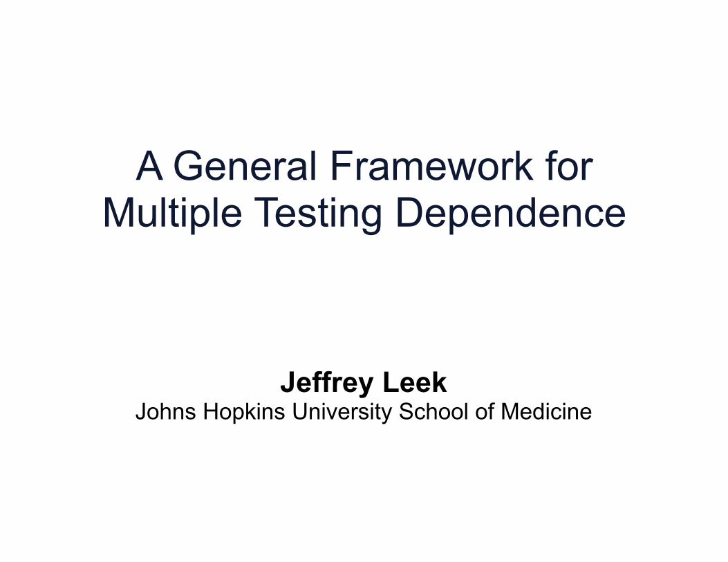
High-dimensional multiple hypothesis testing is common.
Problem: Dependence between tests can result in incorrect statistical and scientific results.
A solution: Define and address multiple testing dependence at the level of the data – not the P-values.
Big Picture Ideas

High-Dimensional Multiple Testing Is Common
Spatial Epidemiology Brain Imaging
Molecular Biology

4
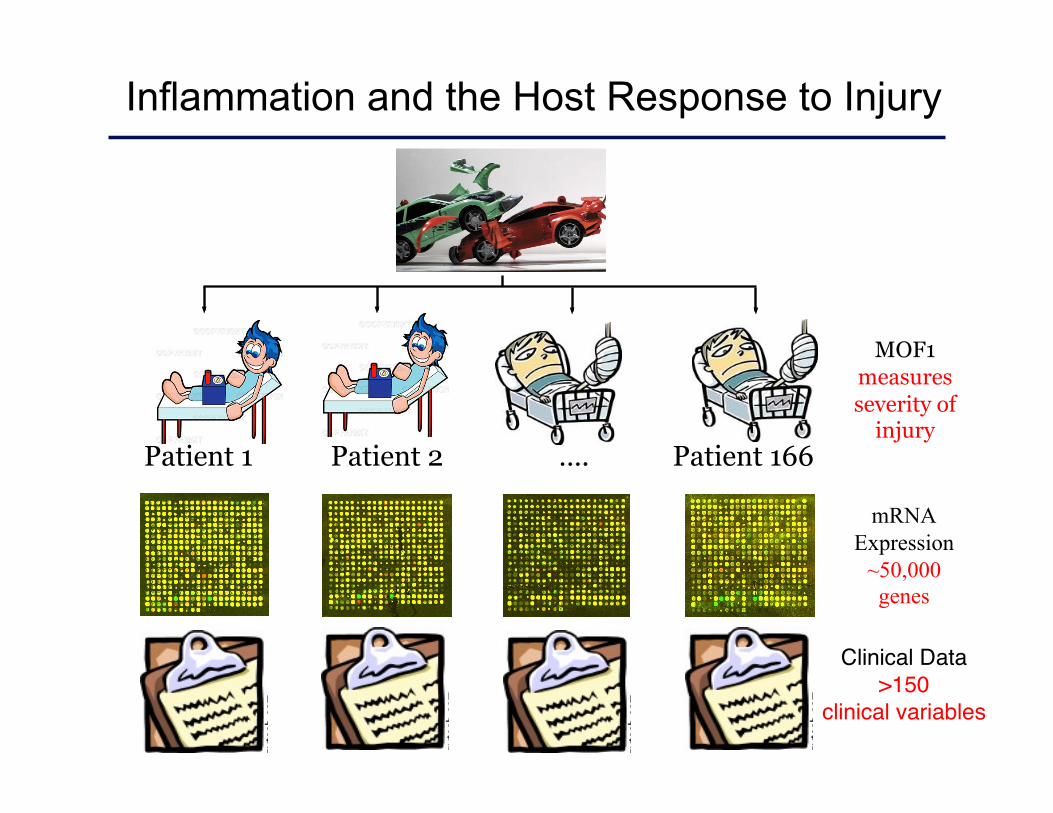
Inflammation and the Host Response to Injury
mRNA Expression
~50,000 genes
Clinical Data >150
clinical variables
Patient 1 Patient 2 Patient 166 ….
MOF measures severity of
injury
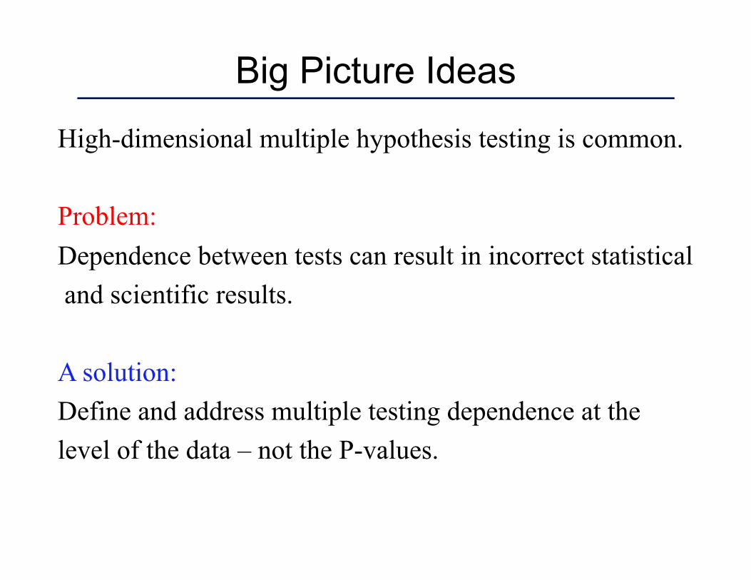
Data at Initial Time Point
Multiple Organ Failure
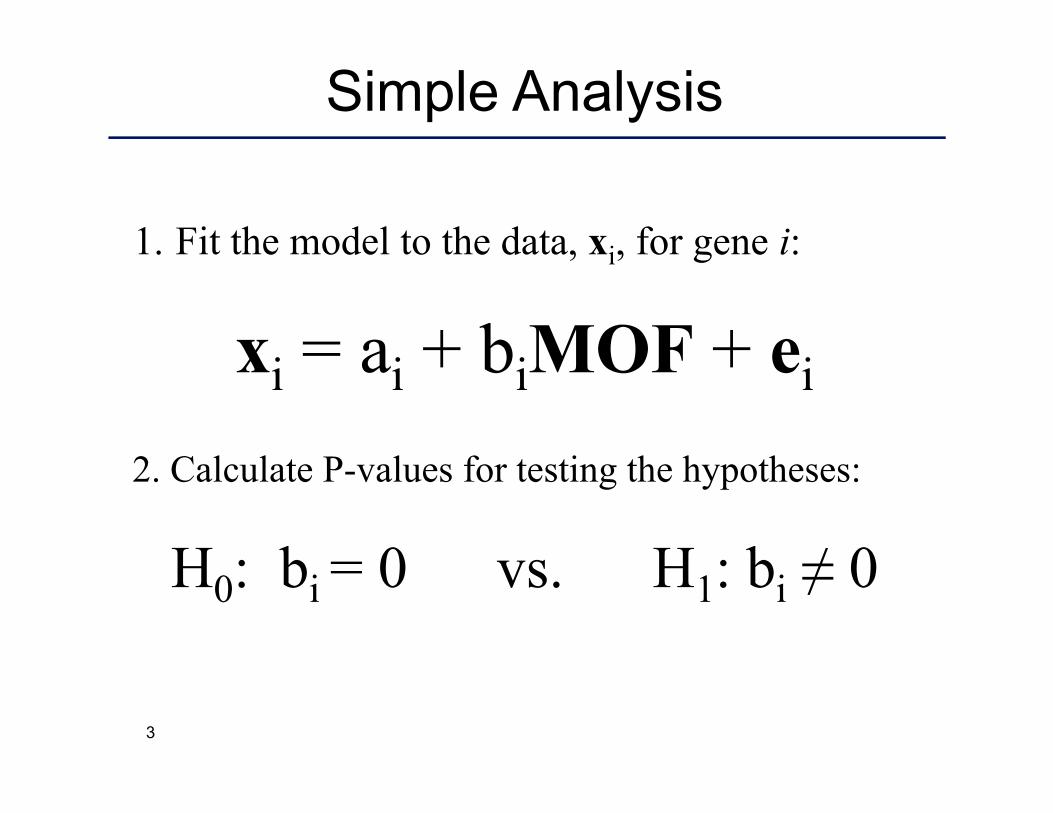
Simple Analysis
1. Fit the model to the data, xi, for gene i:
xi = ai + biMOF + ei
2. Calculate P-values for testing the hypotheses:
H0: bi = 0 vs. H1: bi ≠ 0
3
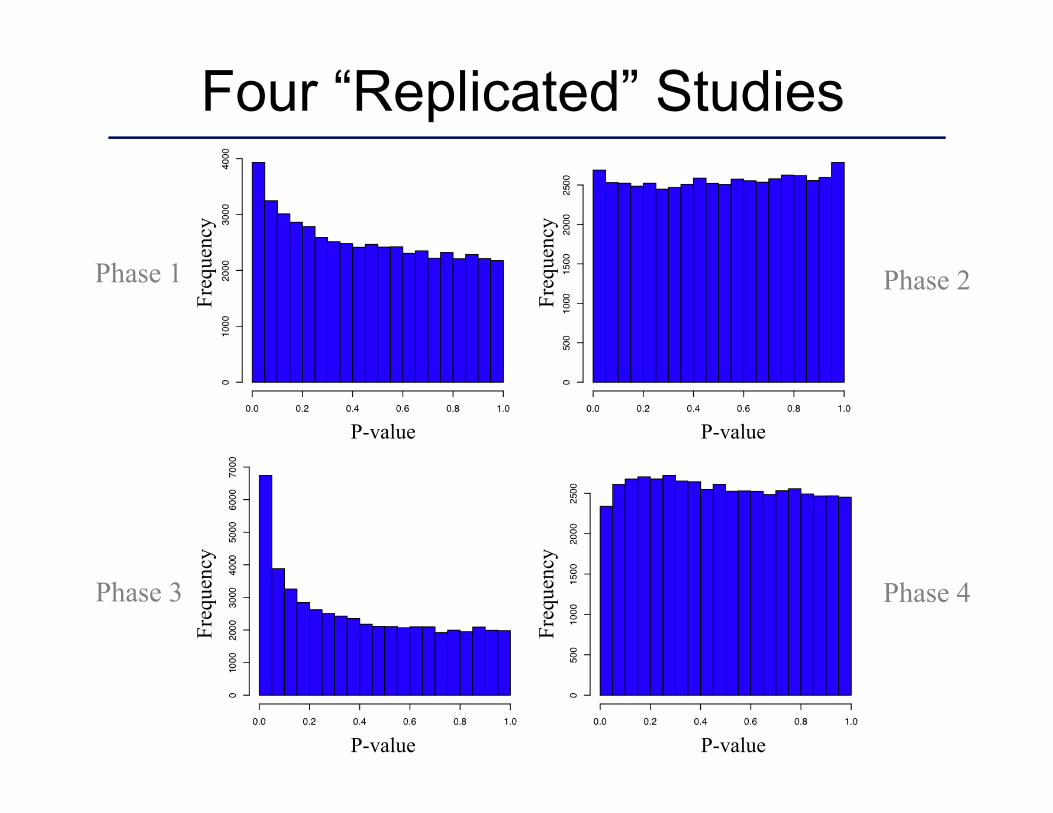
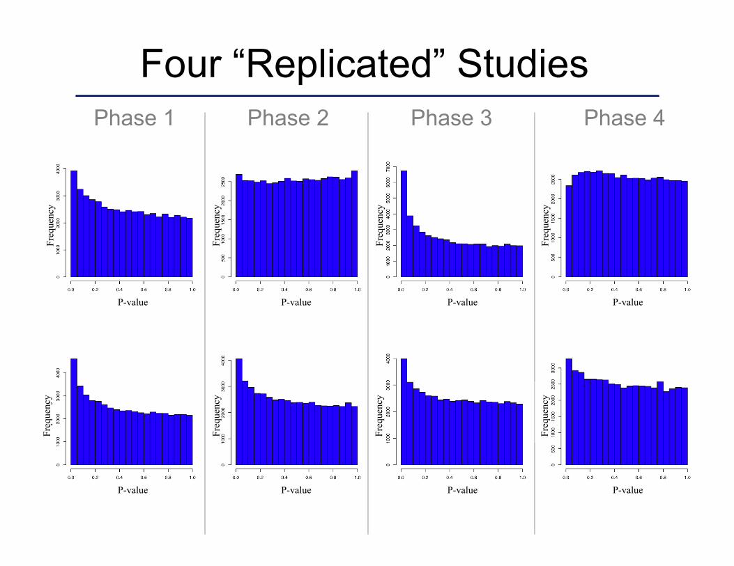
Four “Replicated” Studies
Phase 1
Phase 3
Phase 2
Phase 4
P-value P-value
P-value P-value
Freq
uenc
y
Freq
uenc
y
Freq
uenc
y
Freq
uenc
y
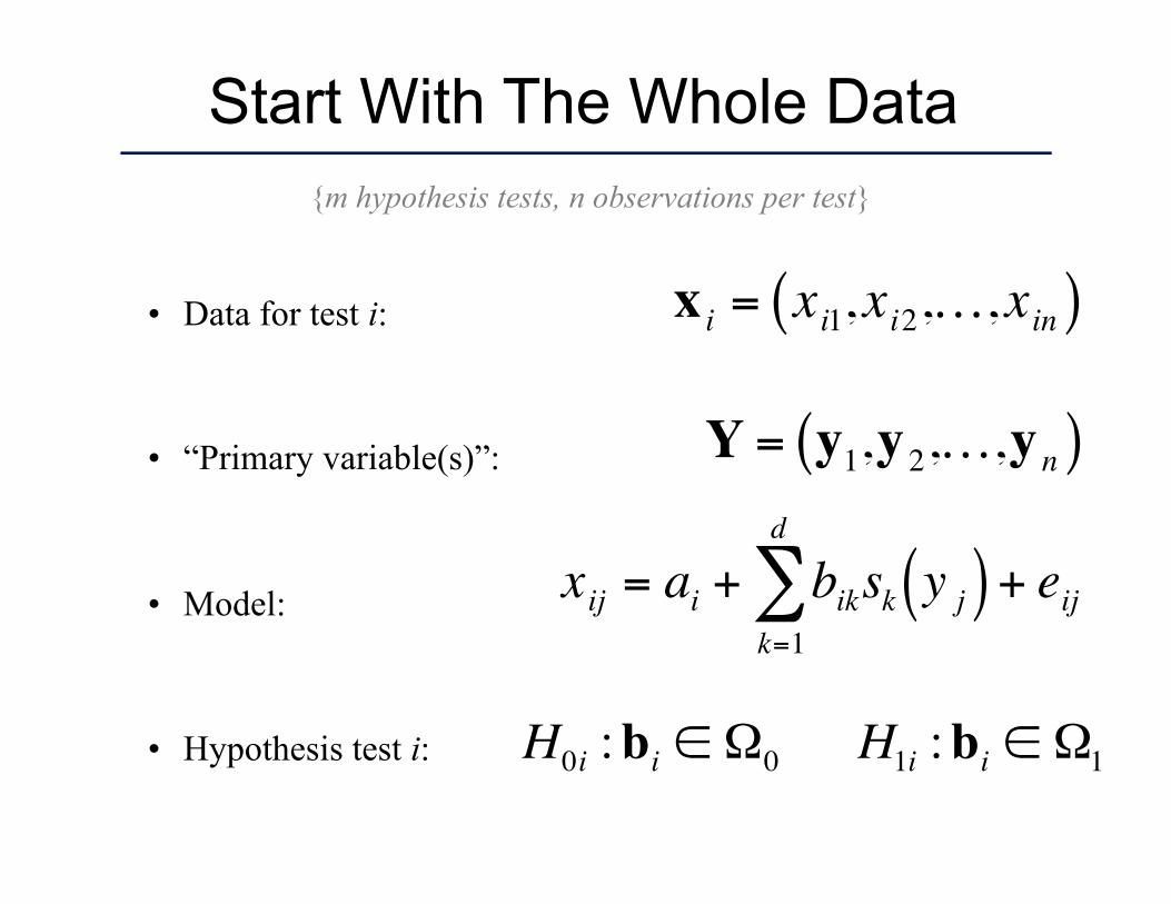
• Data for test i:
• “Primary variable(s)”:
• Model:
• Hypothesis test i:
€
x i = xi1,xi2,…,xin( )
€
Y = y1,y2,…,yn( )
€
xij = ai + biksk y j( )k=1
d
∑ + eij
€
H0i :bi ∈ Ω0 H1i :bi ∈ Ω1
{m hypothesis tests, n observations per test}
Start With The Whole Data
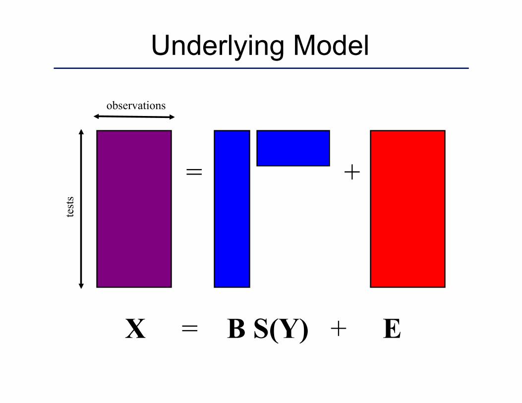
= +
X = B S(Y) + E
observations
test
s Underlying Model
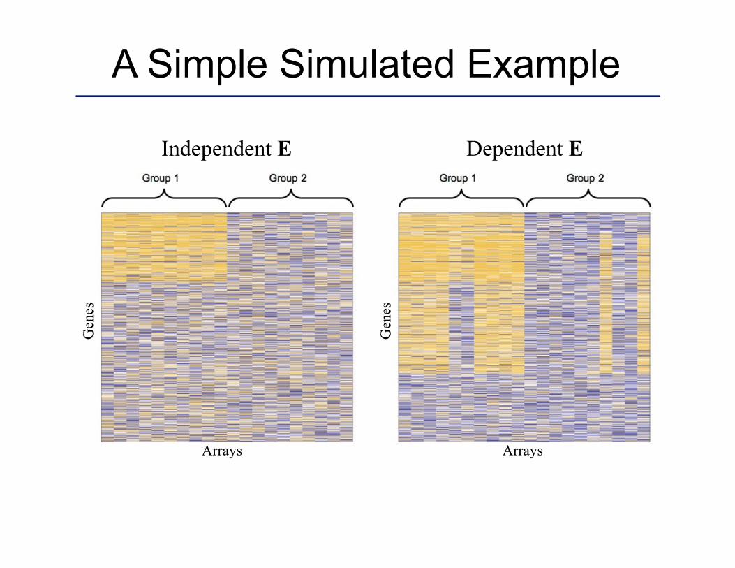
A Simple Simulated Example
Independent E Dependent E
Gen
es
Gen
es
Arrays Arrays
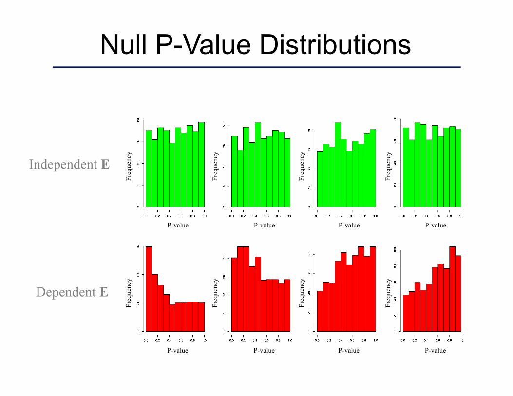
Null P-Value Distributions
Independent E
Dependent E
Freq
uenc
y
Freq
uenc
y
Freq
uenc
y
Freq
uenc
y
Freq
uenc
y
Freq
uenc
y
Freq
uenc
y
Freq
uenc
y
P-value P-value P-value P-value
P-value P-value P-value P-value

Null P-Value Distributions |ρ| = 0.40 |ρ| = 0.31 |ρ| = 0.10 |ρ| = 0.00 Correlation
Independent E
Dependent E
Freq
uenc
y
Freq
uenc
y
Freq
uenc
y
Freq
uenc
y
Freq
uenc
y
Freq
uenc
y
Freq
uenc
y
Freq
uenc
y
P-value P-value P-value P-value
P-value P-value P-value P-value
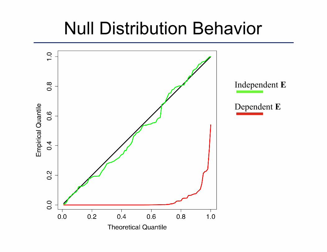
Null Distribution Behavior
Dependent E
Independent E
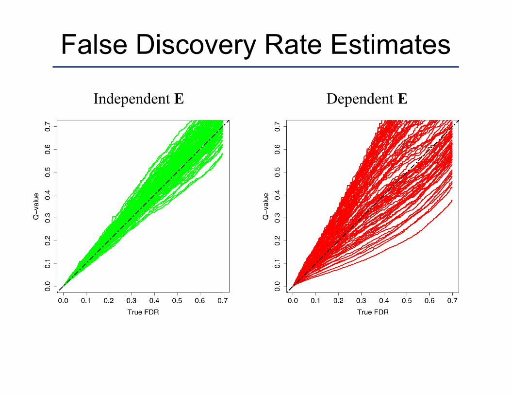
False Discovery Rate Estimates
Independent E Dependent E
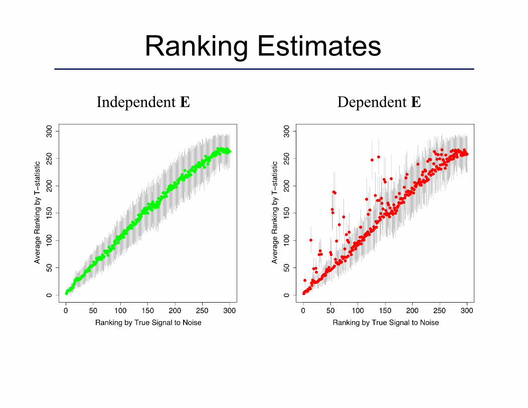
Ranking Estimates
Independent E Dependent E

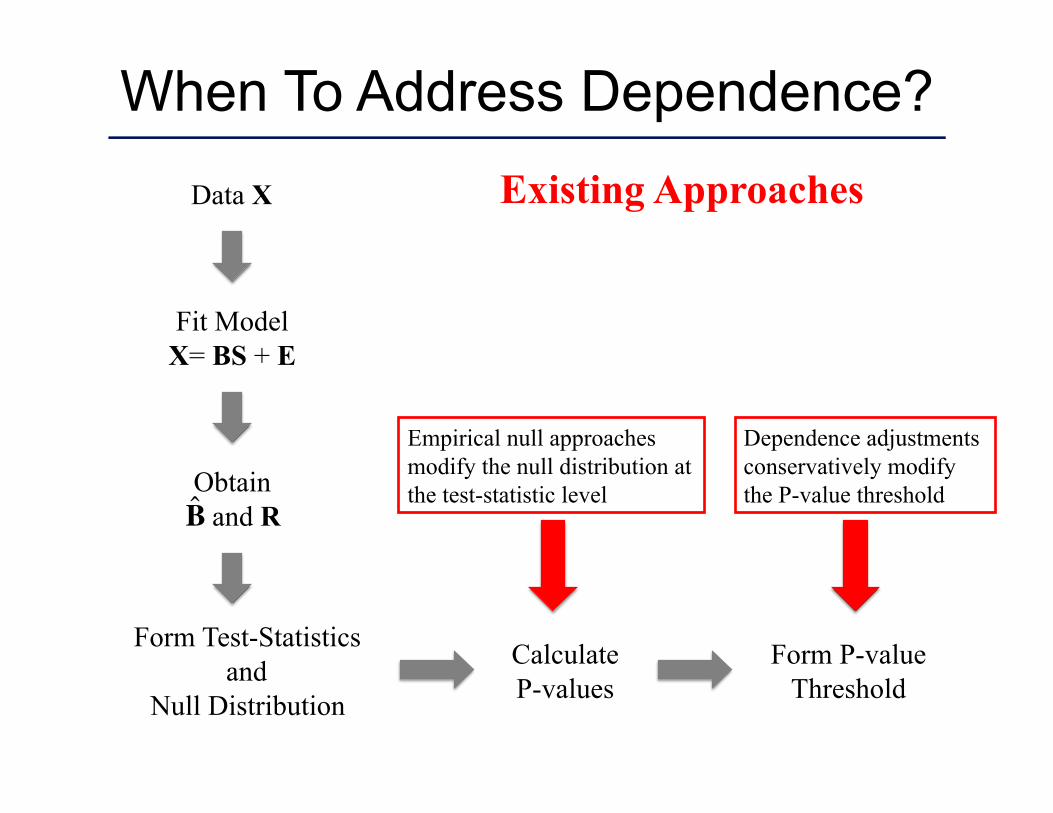
Data X
Fit Model X= BS + E
Obtain and R
€
ˆ B
Calculate P-values
Form P-value Threshold
When To Address Dependence?
Form Test-Statistics and
Null Distribution
Data X
Fit Model X= BS + E
Obtain and R
€
ˆ B
Calculate P-values
Form P-value Threshold
When To Address Dependence?
Form Test-Statistics and
Null Distribution
Existing Approaches
Empirical null approaches modify the null distribution at the test-statistic level
Dependence adjustments conservatively modify the P-value threshold
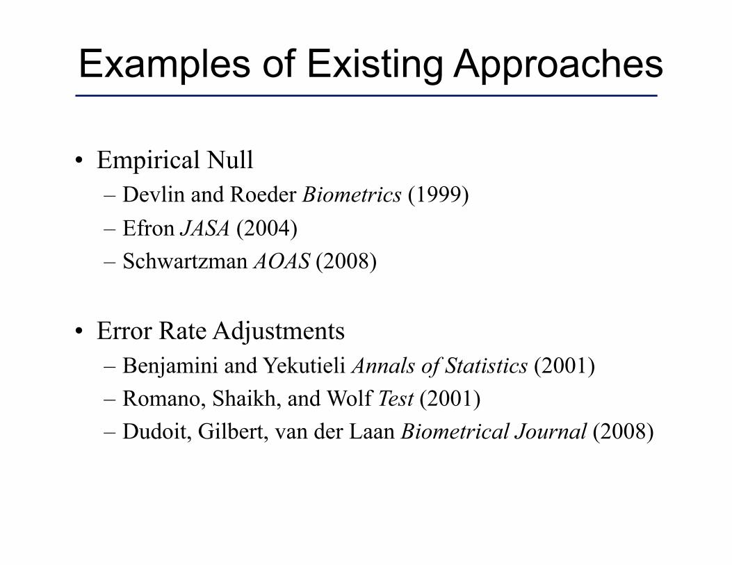
Examples of Existing Approaches
• Empirical Null – Devlin and Roeder Biometrics (1999) – Efron JASA (2004) – Schwartzman AOAS (2008)
• Error Rate Adjustments – Benjamini and Yekutieli Annals of Statistics (2001) – Romano, Shaikh, and Wolf Test (2001) – Dudoit, Gilbert, van der Laan Biometrical Journal (2008)
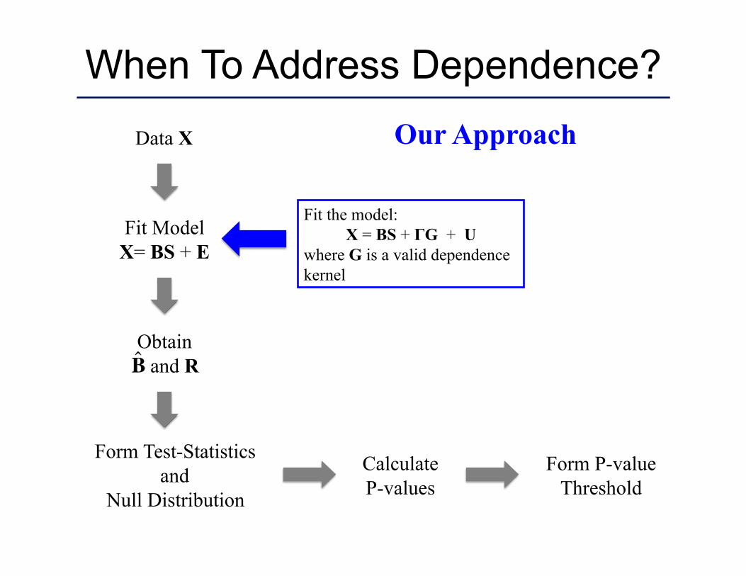
Data X
Fit Model X= BS + E
Obtain and R
€
ˆ B
Calculate P-values
Form P-value Threshold
When To Address Dependence?
Form Test-Statistics and
Null Distribution
Our Approach
Fit the model: X = BS + ΓG + U
where G is a valid dependence kernel
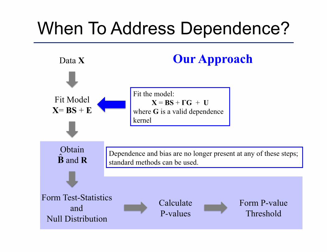
Dependence and bias are no longer present at any of these steps; standard methods can be used.
Data X
Fit Model X= BS + E
Obtain and R
€
ˆ B
Calculate P-values
Form P-value Threshold
When To Address Dependence?
Form Test-Statistics and
Null Distribution
Our Approach
Fit the model: X = BS + ΓG + U
where G is a valid dependence kernel
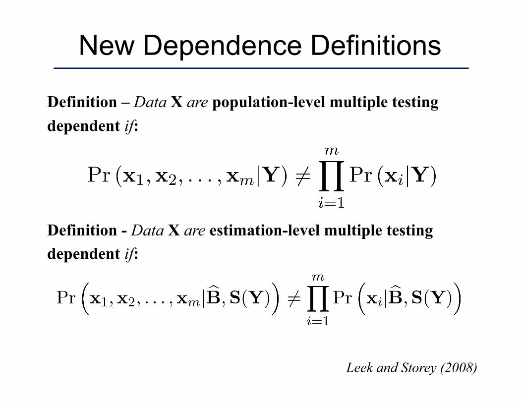
New Dependence Definitions
Definition – Data X are population-level multiple testing dependent if:
Definition - Data X are estimation-level multiple testing dependent if:
Leek and Storey (2008)
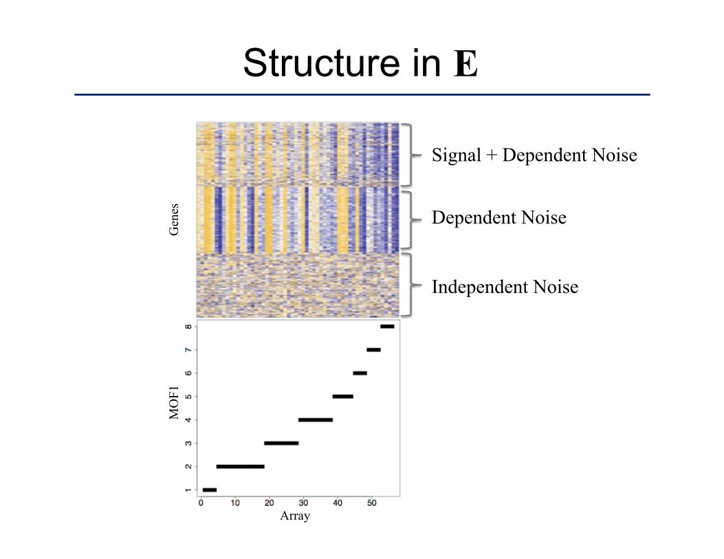
Structure in E
Array
MO
F1
Gen
es
Signal + Dependent Noise
Dependent Noise
Independent Noise
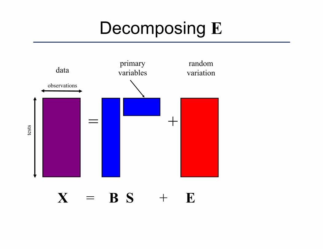
= +
X = B S + E
observations
test
s
data random variation
primary variables
Decomposing E
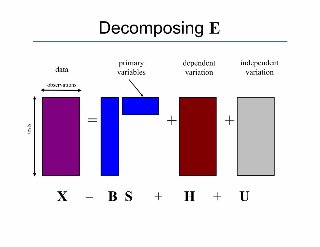
= +
X = B S + H + U
test
s +
independent variation
observations
data primary variables
dependent variation
Decomposing E
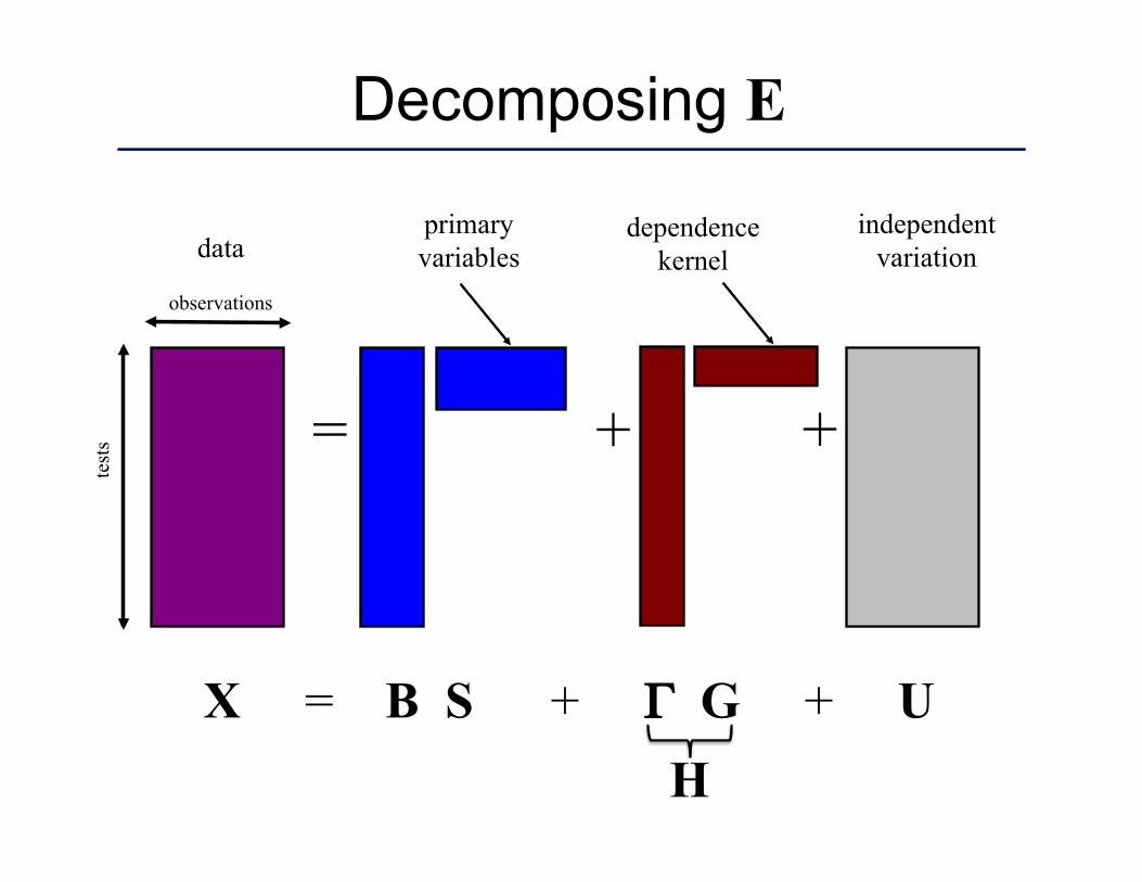
= +
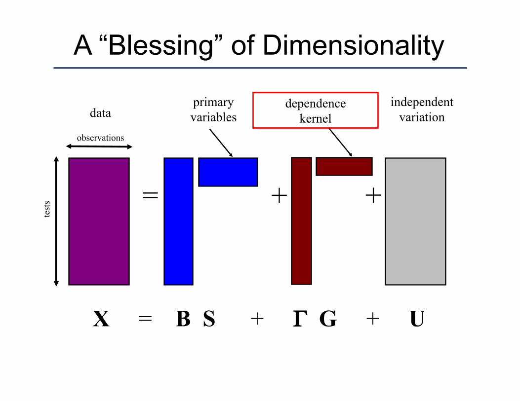
X = B S + Γ G + U
test
s +
independent variation
observations
data primary variables
dependence kernel
Decomposing E
H
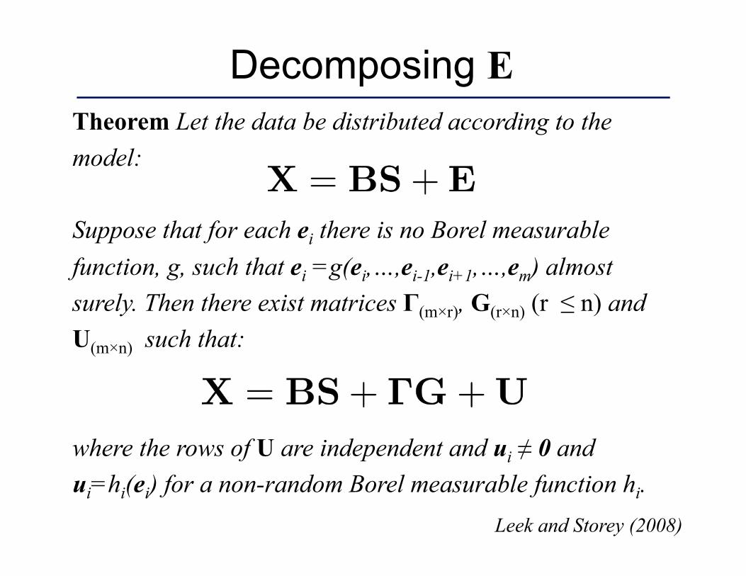
Decomposing E Theorem Let the data be distributed according to the model:
Suppose that for each ei there is no Borel measurable function, g, such that ei =g(ei,…,ei-1,ei+1,…,em) almost surely. Then there exist matrices Γ(m×r), G(r×n) (r ≤ n) and U(m×n) such that:
where the rows of U are independent and ui ≠ 0 and ui=hi(ei) for a non-random Borel measurable function hi.
Leek and Storey (2008)
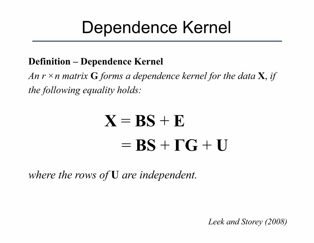
Dependence Kernel
Leek and Storey (2008)
Definition – Dependence Kernel An r ×n matrix G forms a dependence kernel for the data X, if the following equality holds:
X = BS + E = BS + ΓG + U where the rows of U are independent.
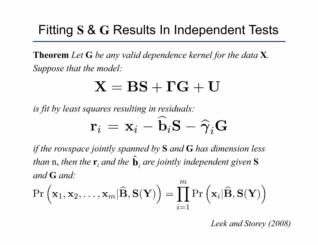
Fitting S & G Results In Independent Tests
Leek and Storey (2008)
Theorem Let G be any valid dependence kernel for the data X. Suppose that the model:
is fit by least squares resulting in residuals:
if the rowspace jointly spanned by S and G has dimension less than n, then the ri and the are jointly independent given S and G and:
€
ˆ b i
= +
X = B S + Γ G + U
test
s +
independent variation
observations
data primary variables
dependence kernel
A “Blessing” of Dimensionality
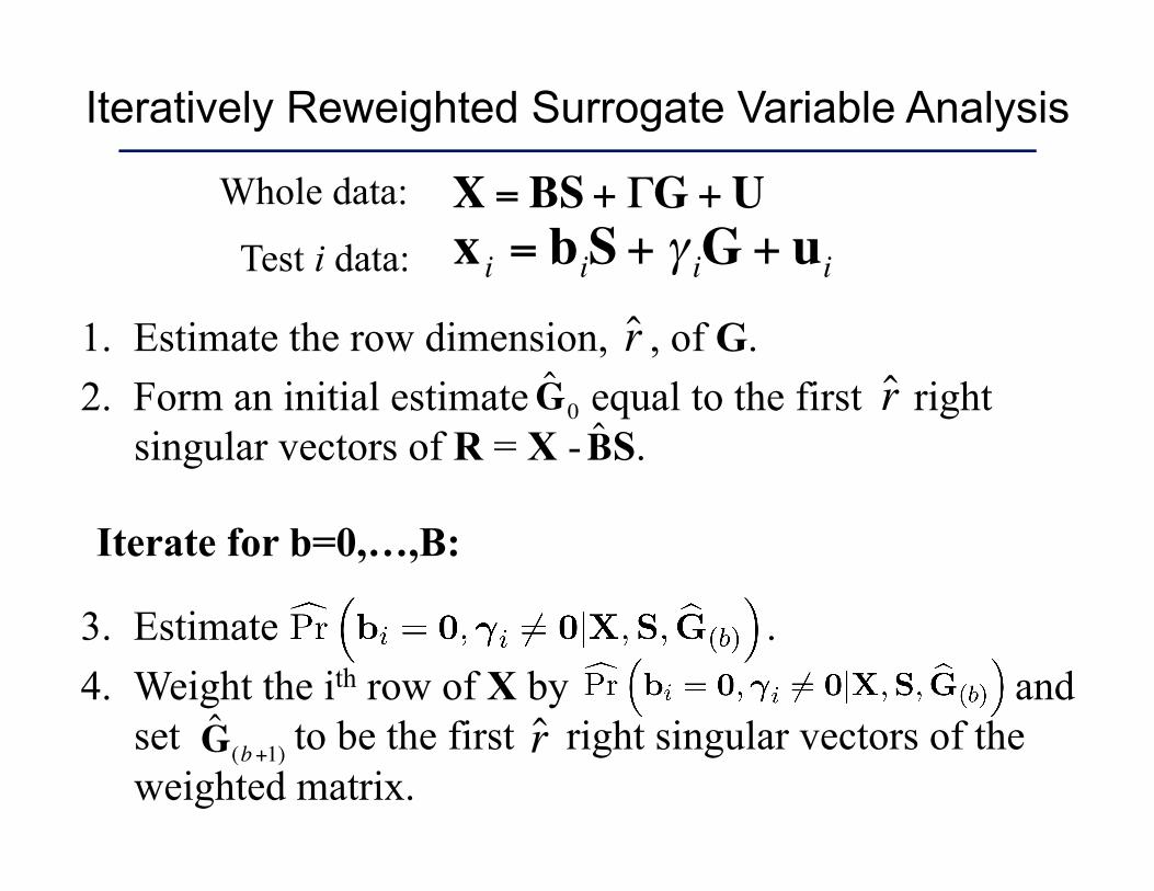
Iteratively Reweighted Surrogate Variable Analysis
1. Estimate the row dimension, , of G. 2. Form an initial estimate equal to the first right
singular vectors of R = X - S.
3. Estimate . 4. Weight the ith row of X by and
set to be the first right singular vectors of the weighted matrix.
€
ˆ G (b+1)
€
ˆ r
€
ˆ B
Iterate for b=0,…,B: €
ˆ G 0
€
ˆ r
€
X = BS+ ΓG +U
€
x i = biS+ γ iG + uiWhole data:
Test i data:
€
ˆ r
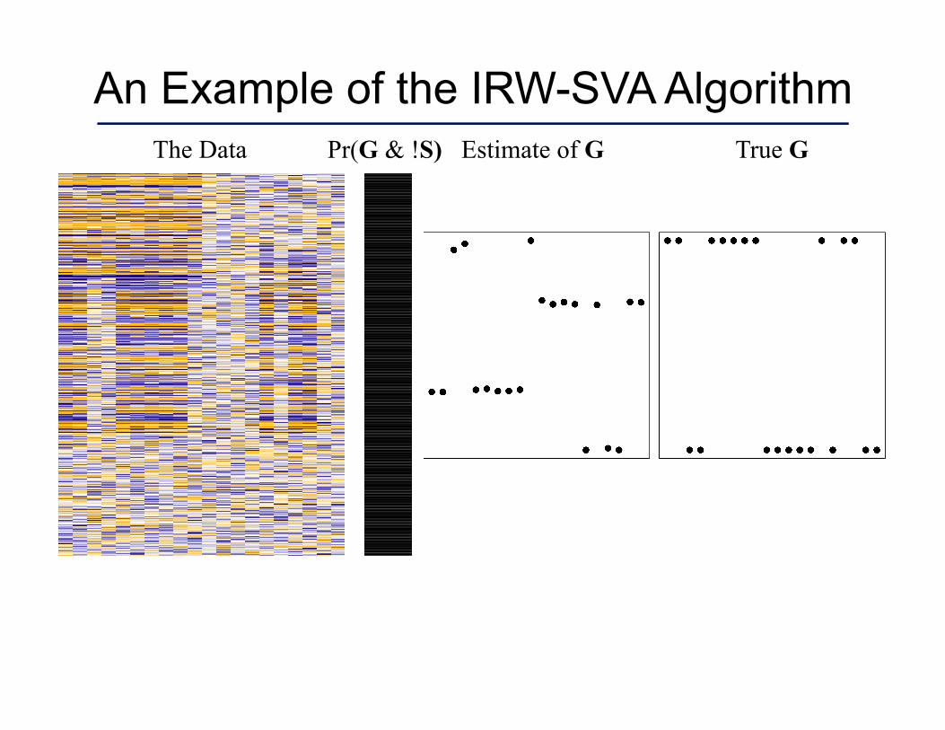
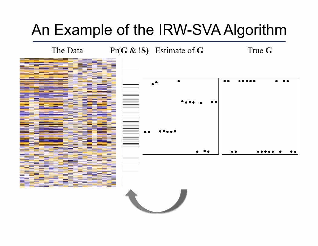
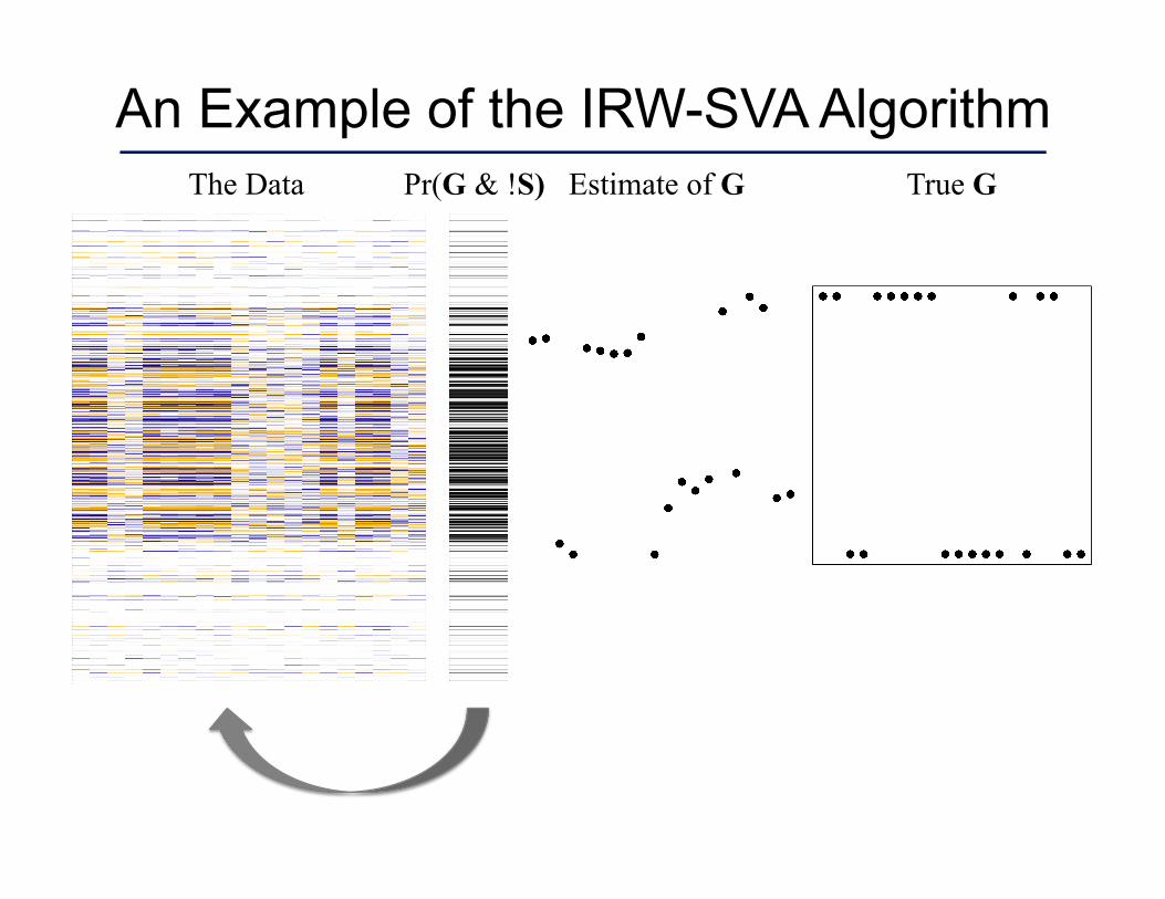
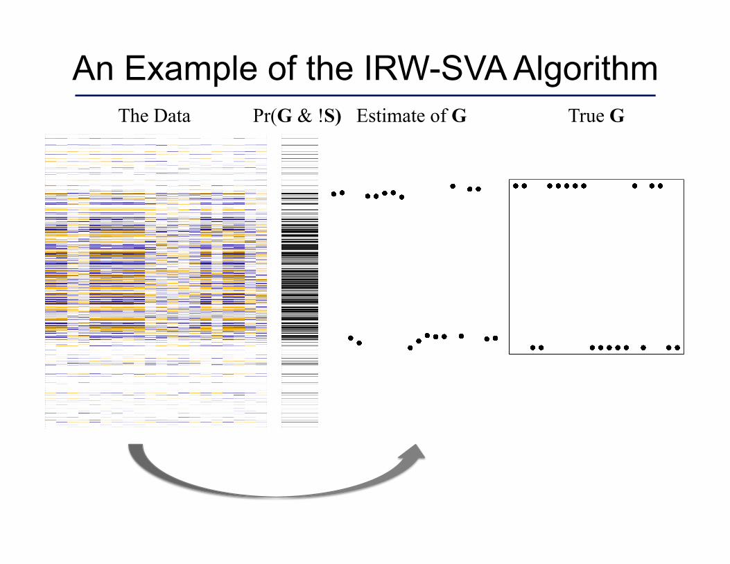
An Example of the IRW-SVA Algorithm The Data True G Estimate of G Pr(G & !S)
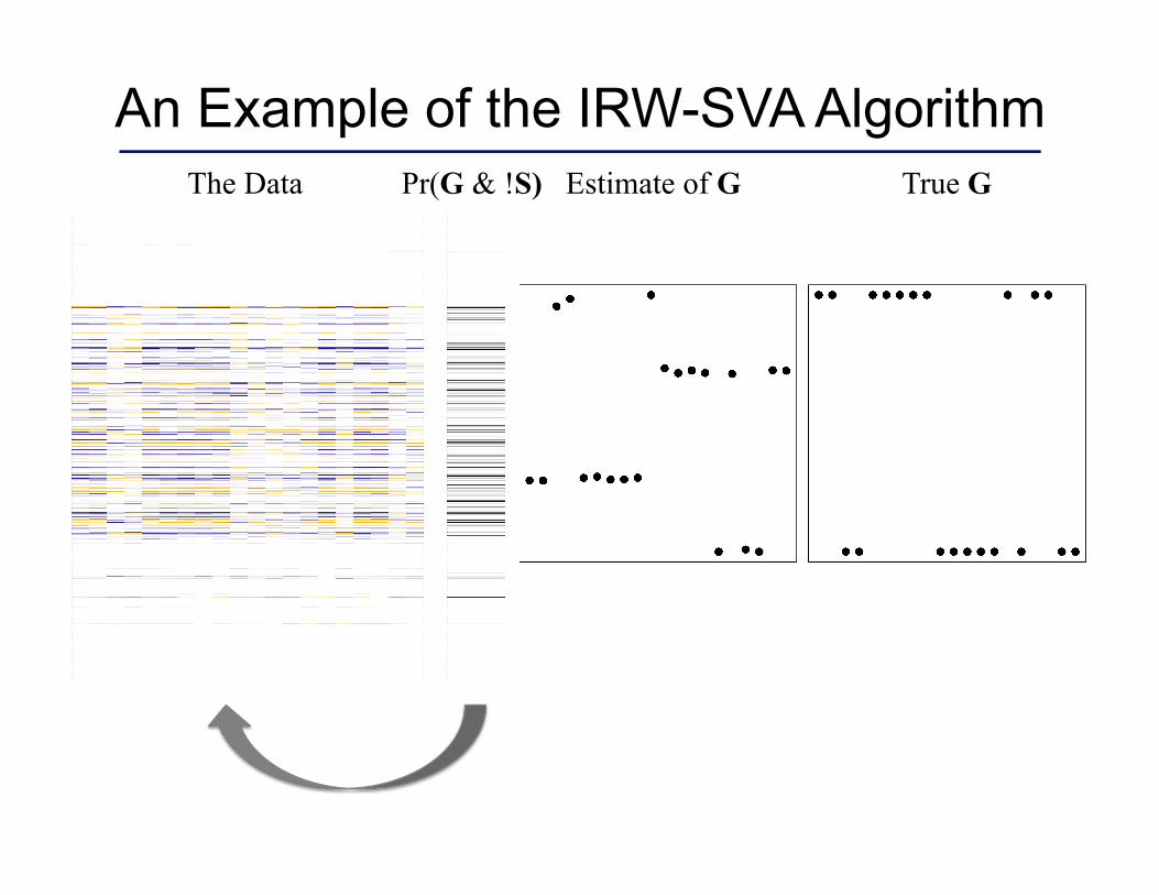
An Example of the IRW-SVA Algorithm The Data True G Estimate of G Pr(G & !S)
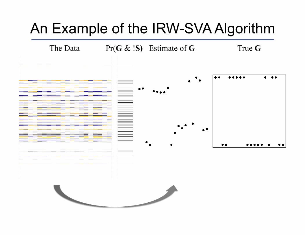
An Example of the IRW-SVA Algorithm The Data True G Estimate of G Pr(G & !S)
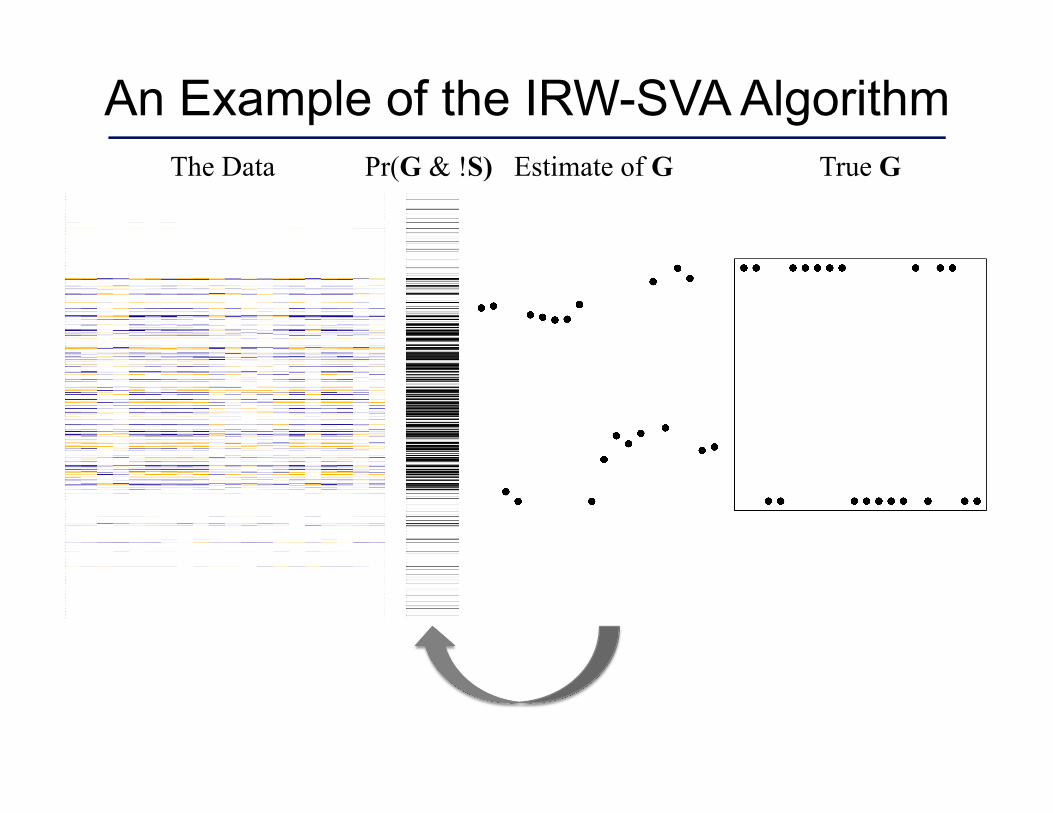
An Example of the IRW-SVA Algorithm The Data True G Estimate of G Pr(G & !S)
An Example of the IRW-SVA Algorithm The Data True G Estimate of G Pr(G & !S)
An Example of the IRW-SVA Algorithm The Data True G Estimate of G Pr(G & !S)
An Example of the IRW-SVA Algorithm The Data True G Estimate of G Pr(G & !S)
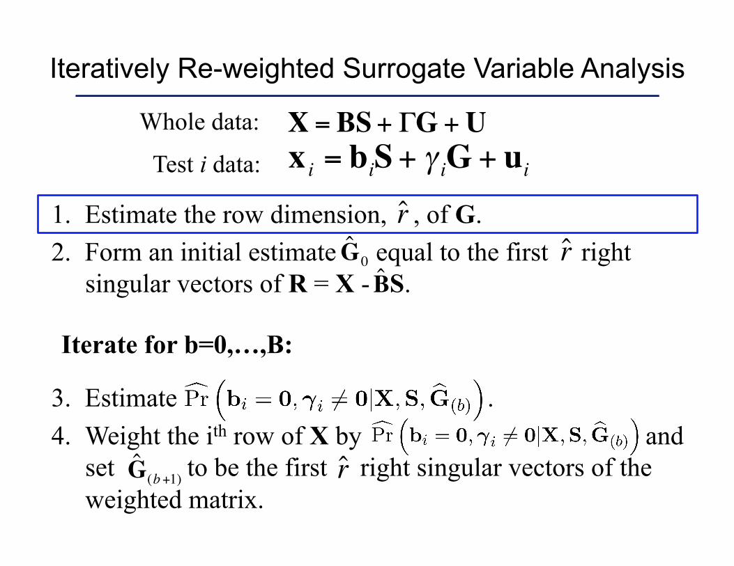
Iteratively Re-weighted Surrogate Variable Analysis
1. Estimate the row dimension, , of G. 2. Form an initial estimate equal to the first right
singular vectors of R = X - S.
3. Estimate . 4. Weight the ith row of X by and
set to be the first right singular vectors of the weighted matrix.
€
ˆ G (b+1)
€
ˆ r
€
ˆ B
€
ˆ G 0
€
ˆ r
€
X = BS+ ΓG +U
€
x i = biS+ γ iG + uiWhole data:
Test i data:
€
ˆ r
Iterate for b=0,…,B:
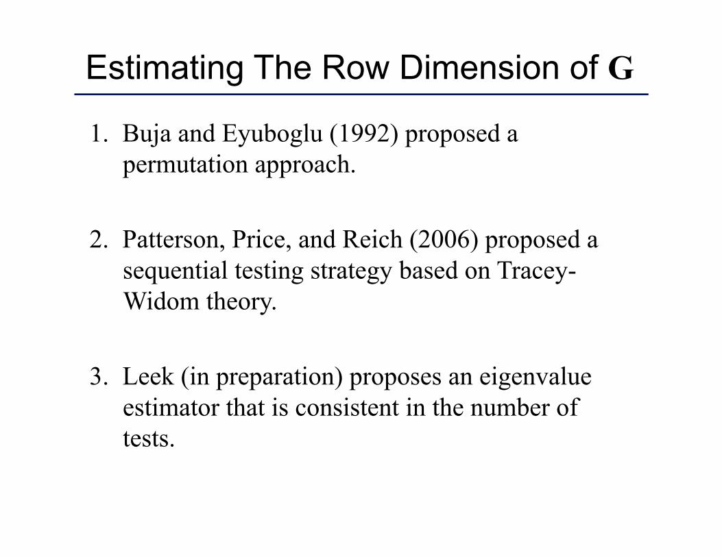
1. Buja and Eyuboglu (1992) proposed a permutation approach.
2. Patterson, Price, and Reich (2006) proposed a sequential testing strategy based on Tracey-Widom theory.
3. Leek (in preparation) proposes an eigenvalue estimator that is consistent in the number of tests.
Estimating The Row Dimension of G
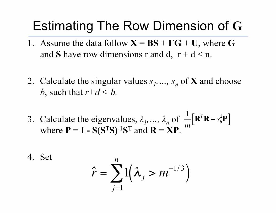
1. Assume the data follow X = BS + ΓG + U, where G and S have row dimensions r and d, r + d < n.
2. Calculate the singular values s1,…, sn of X and choose b, such that r+d < b.
3. Calculate the eigenvalues, λ1,…, λn of where P = I - S(STS)-1ST and R = XP.
4. Set
€
ˆ r = 1 λ j > m−1/ 3( )j=1
n
∑
€
€
1mRTR− sb
2P[ ]
Estimating The Row Dimension of G
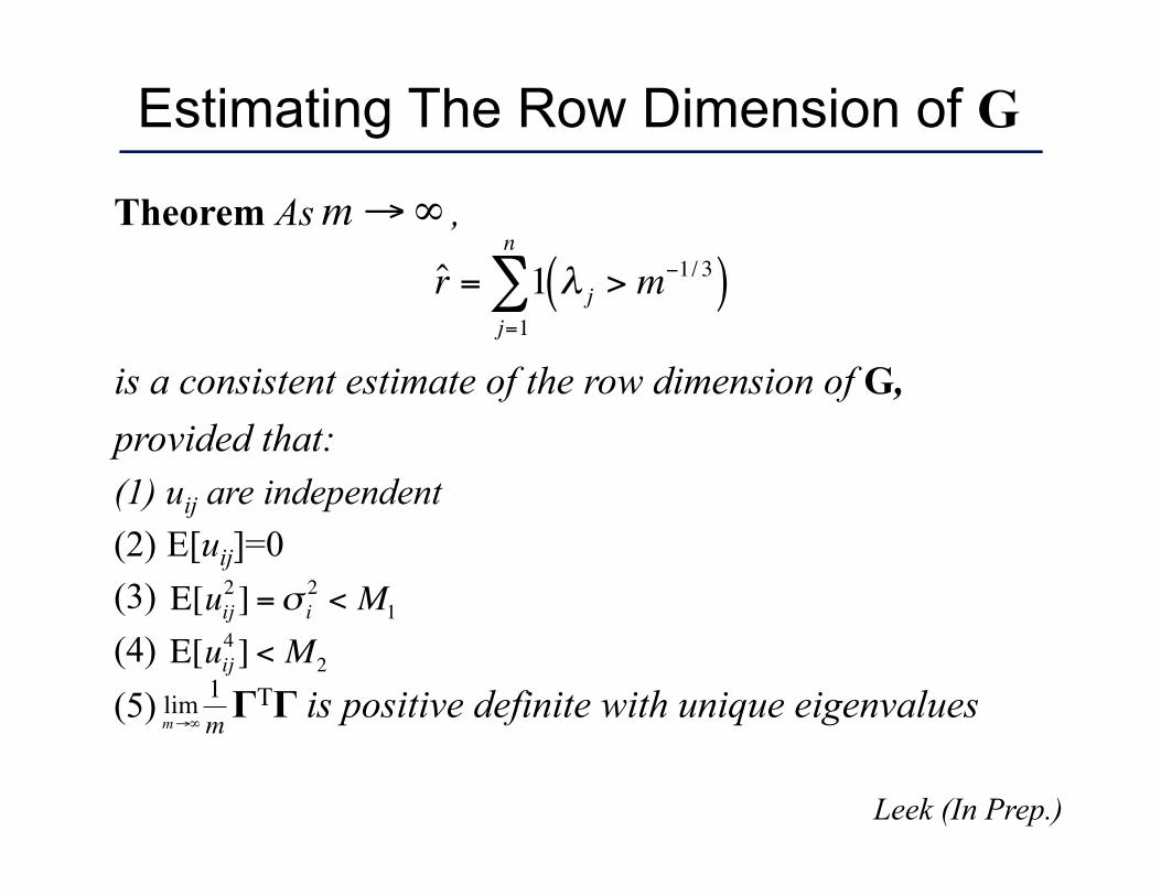
Theorem As ,
is a consistent estimate of the row dimension of G, provided that: (1) uij are independent (2) E[uij]=0 (3) (4) (5) ΓTΓ is positive definite with unique eigenvalues
€
m→∞
€
E[uij2 ] =σ i
2 < M1
€
E[uij4 ] < M2
€
limm→∞
1m
Leek (In Prep.)
€
ˆ r = 1 λ j > m−1/ 3( )j=1
n
∑
Estimating The Row Dimension of G
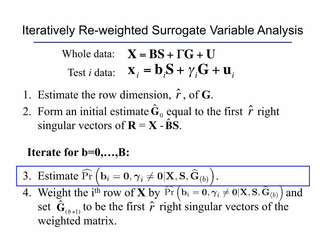
Iteratively Re-weighted Surrogate Variable Analysis
1. Estimate the row dimension, , of G. 2. Form an initial estimate equal to the first right
singular vectors of R = X - S.
3. Estimate . 4. Weight the ith row of X by and
set to be the first right singular vectors of the weighted matrix.
€
ˆ G (b+1)
€
ˆ r
€
ˆ B
€
ˆ G 0
€
ˆ r
€
X = BS+ ΓG +U
€
x i = biS+ γ iG + uiWhole data:
Test i data:
€
ˆ r
Iterate for b=0,…,B:
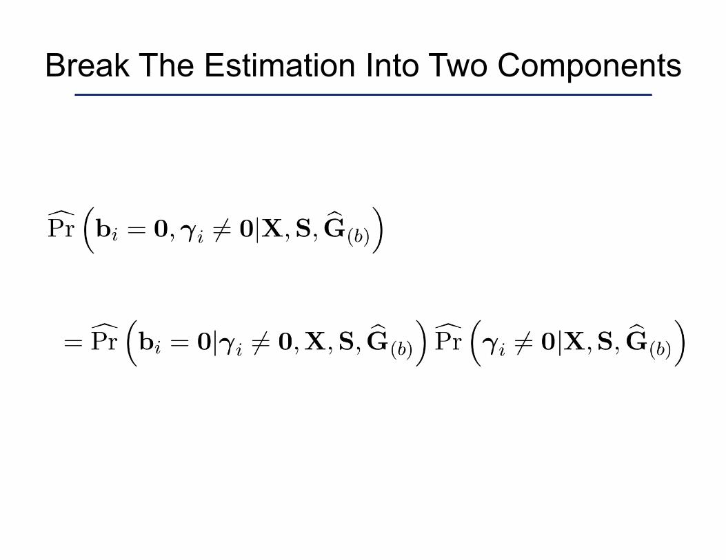
Break The Estimation Into Two Components
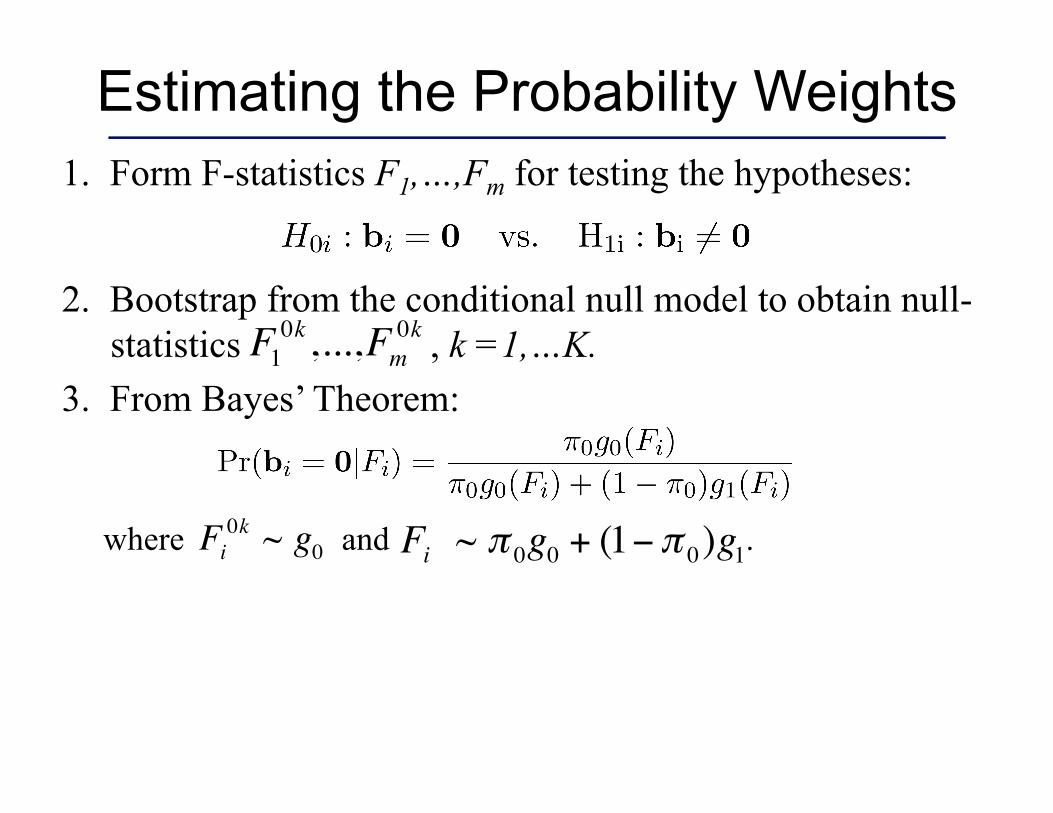
1. Form F-statistics F1,…,Fm for testing the hypotheses:
2. Bootstrap from the conditional null model to obtain null-statistics , k =1,…K.
3. From Bayes’ Theorem:
where and .
Estimating the Probability Weights
€
F10k,...,Fm
0k
€
Fi0k ~ g0
€
Fi ~ π 0g0 + (1−π 0)g1
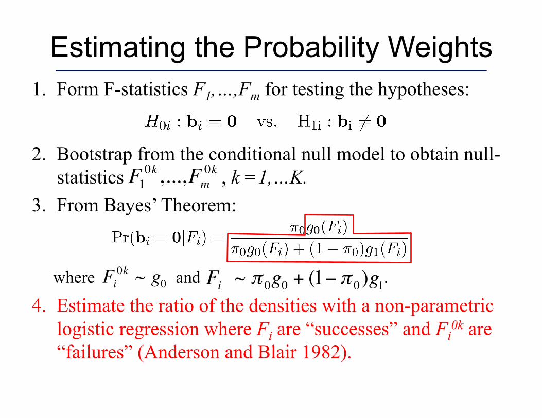
1. Form F-statistics F1,…,Fm for testing the hypotheses:
2. Bootstrap from the conditional null model to obtain null-statistics , k =1,…K.
3. From Bayes’ Theorem:
4. Estimate the ratio of the densities with a non-parametric logistic regression where Fi are “successes” and Fi
0k are “failures” (Anderson and Blair 1982).
where and . .
Estimating the Probability Weights
€
F10k,...,Fm
0k
€
Fi0k ~ g0
€
Fi ~ π 0g0 + (1−π 0)g1
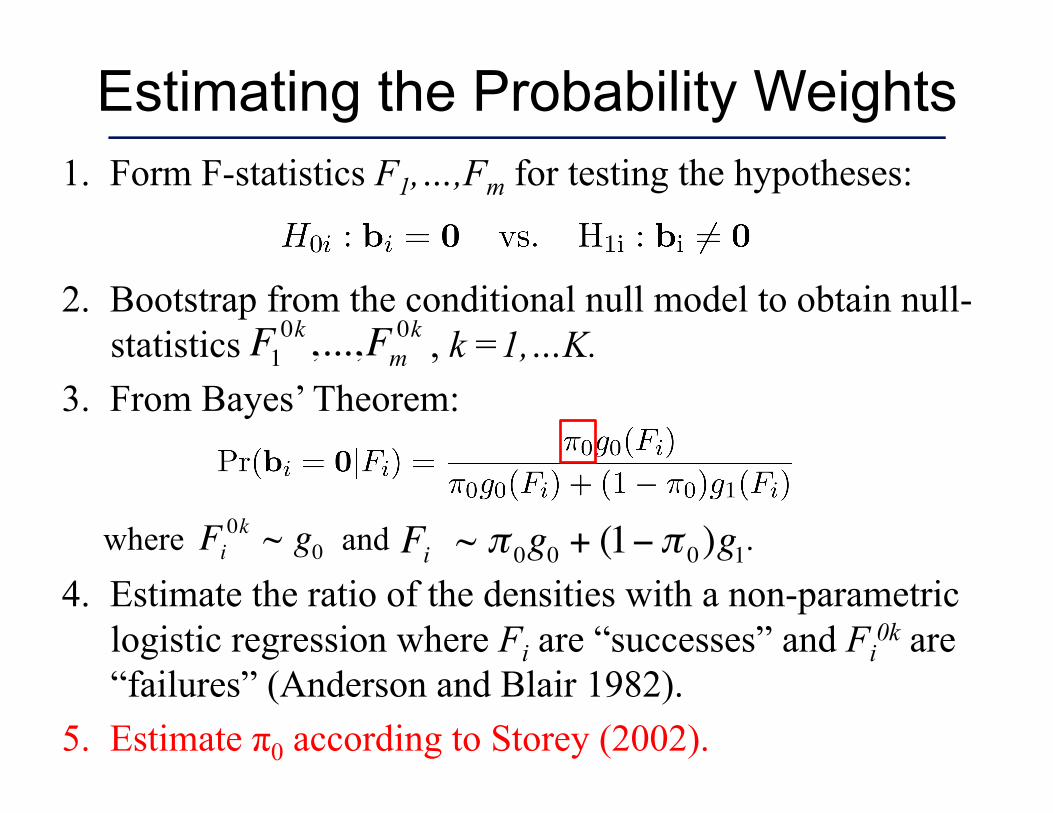
1. Form F-statistics F1,…,Fm for testing the hypotheses:
2. Bootstrap from the conditional null model to obtain null-statistics , k =1,…K.
3. From Bayes’ Theorem:
4. Estimate the ratio of the densities with a non-parametric logistic regression where Fi are “successes” and Fi
0k are “failures” (Anderson and Blair 1982).
5. Estimate π0 according to Storey (2002).
where and .
Estimating the Probability Weights
€
F10k,...,Fm
0k
€
Fi0k ~ g0
€
Fi ~ π 0g0 + (1−π 0)g1
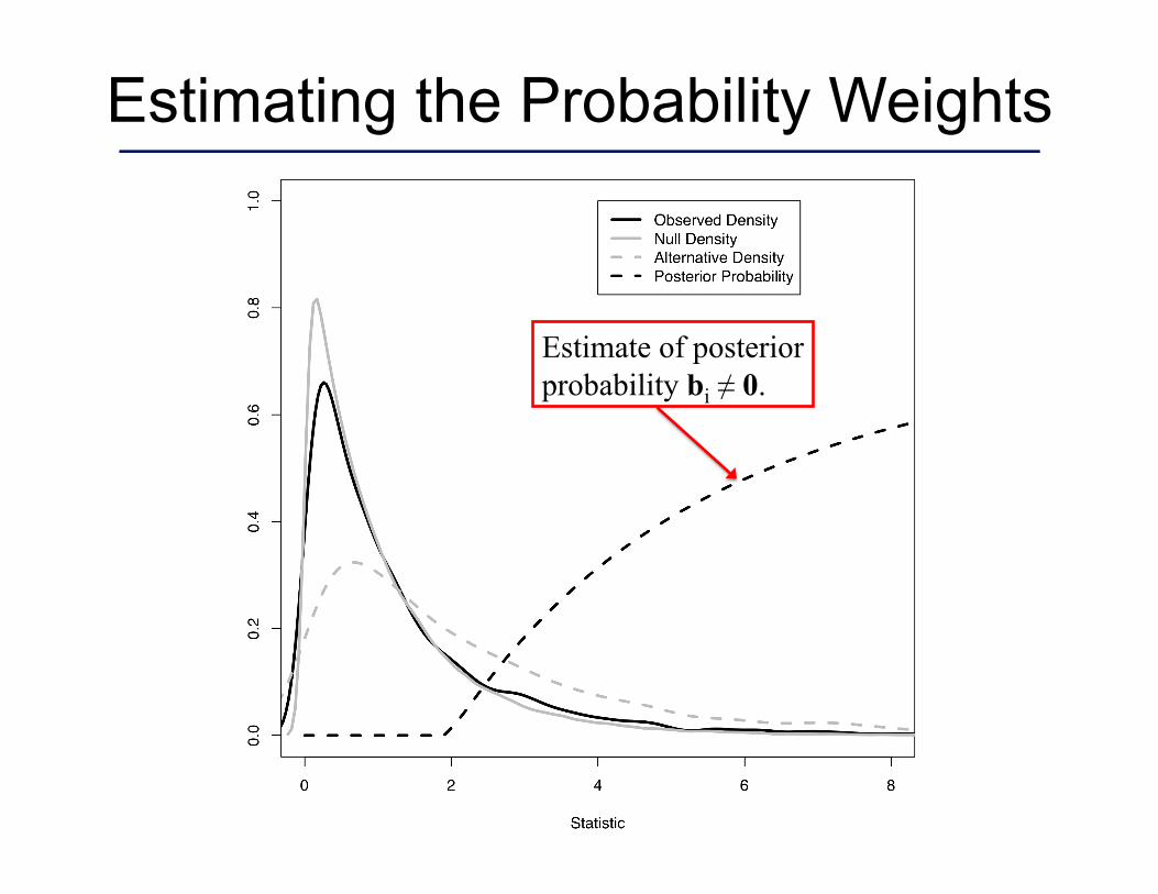
Estimating the Probability Weights
Estimate of posterior probability bi ≠ 0.
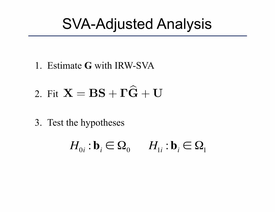
SVA-Adjusted Analysis
1. Estimate G with IRW-SVA
2. Fit
3. Test the hypotheses
€
H0i :bi ∈ Ω0 H1i :bi ∈ Ω1

A Simple Simulated Example
Independent E Dependent E
Gen
es
Gen
es
Arrays Arrays
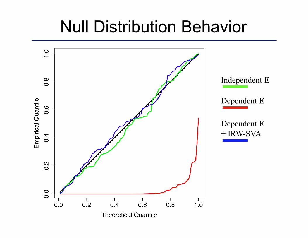
Null Distribution Behavior
Dependent E
Independent E
Dependent E + IRW-SVA
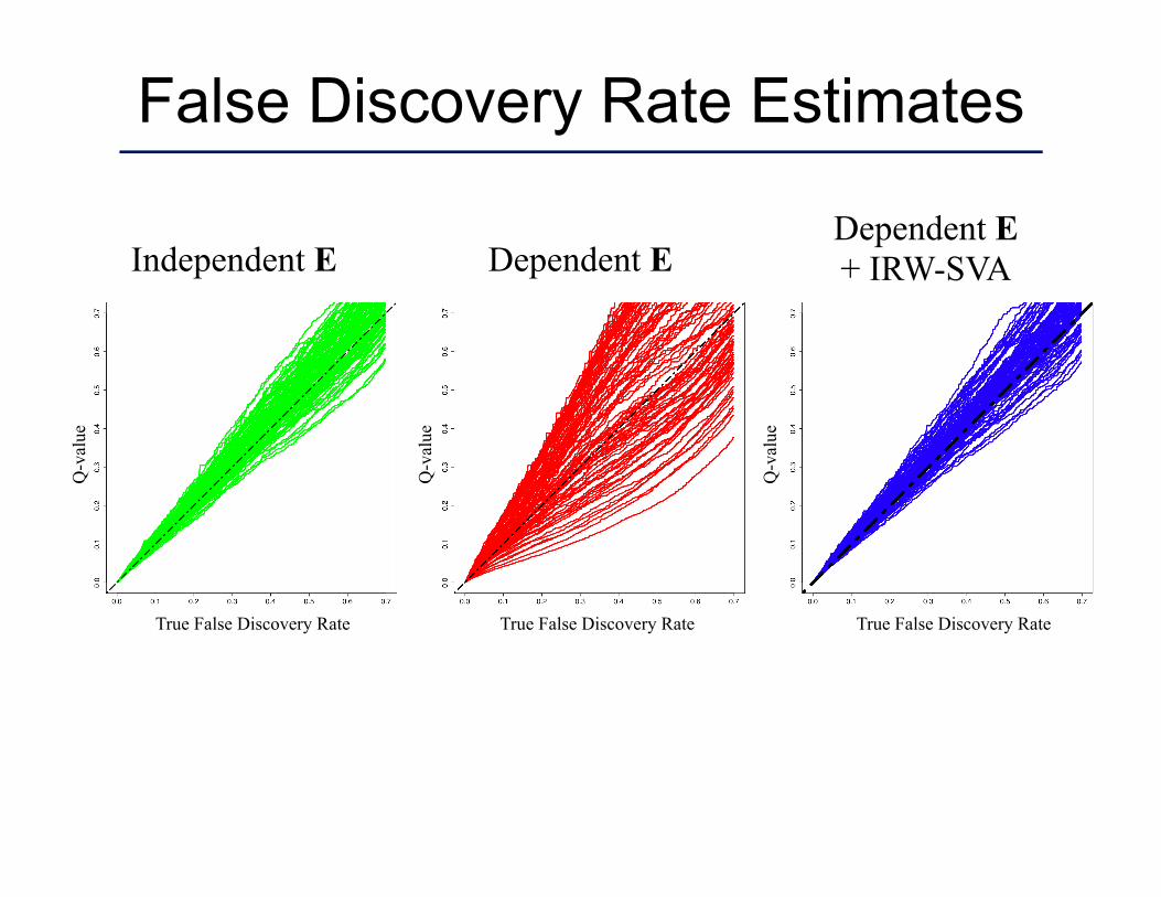
False Discovery Rate Estimates
Independent E Dependent E Dependent E + IRW-SVA
True False Discovery Rate True False Discovery Rate True False Discovery Rate
Q-v
alue
Q-v
alue
Q-v
alue
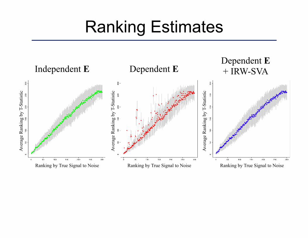
Ranking Estimates
Independent E Dependent E Dependent E + IRW-SVA
Ranking by True Signal to Noise Ranking by True Signal to Noise Ranking by True Signal to Noise
Aver
age
Ran
king
by
T-St
atis
tic
Aver
age
Ran
king
by
T-St
atis
tic
Aver
age
Ran
king
by
T-St
atis
tic
53
Inflammation and the Host Response to Injury
mRNA Expression
~50,000 genes
Clinical Data >150
clinical variables
Patient 1 Patient 2 Patient 166 ….
MOF1 measures severity of
injury
Phase 1 Phase 2 Phase 3 Phase 4
Four “Replicated” Studies Fr
eque
ncy
Freq
uenc
y
P-value P-value P-value P-value
P-value P-value P-value P-value
Freq
uenc
y
Freq
uenc
y
Freq
uenc
y
Freq
uenc
y
Freq
uenc
y
Freq
uenc
y
Freq
uenc
y
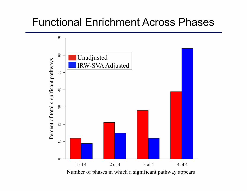
Functional Enrichment Across Phases
Number of phases in which a significant pathway appears
Perc
ent o
f tot
al si
gnifi
cant
pat
hway
s
1 of 4 2 of 4 3 of 4 4 of 4
Unadjusted IRW-SVA Adjusted
• High-dimensional hypothesis testing is common.
• Dependence between tests can result in incorrect statistical and scientific inference.
• We can define and address dependence at the level of the model using the dependence kernel.
• IRW-SVA can be used to improve inference in high-dimensional multiple hypothesis testing.
Summary
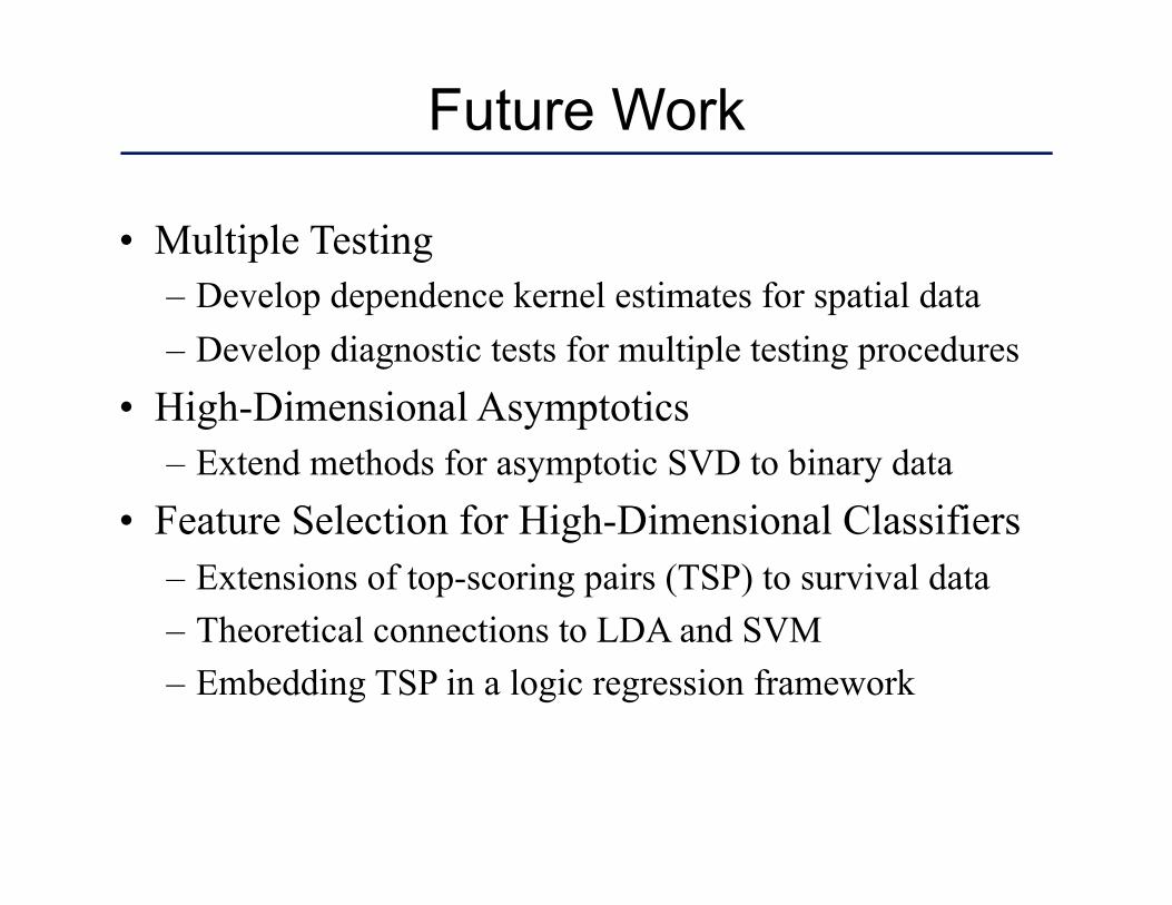
Future Work
• Multiple Testing – Develop dependence kernel estimates for spatial data – Develop diagnostic tests for multiple testing procedures
• High-Dimensional Asymptotics – Extend methods for asymptotic SVD to binary data
• Feature Selection for High-Dimensional Classifiers – Extensions of top-scoring pairs (TSP) to survival data – Theoretical connections to LDA and SVM – Embedding TSP in a logic regression framework

Thank You
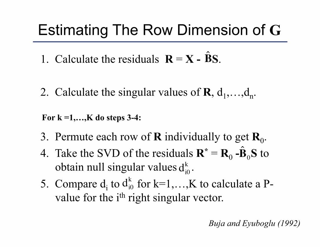
1. Calculate the residuals R = X - S.
2. Calculate the singular values of R, d1,…,dn.
3. Permute each row of R individually to get R0. 4. Take the SVD of the residuals R* = R0 - S to
obtain null singular values . 5. Compare di to for k=1,…,K to calculate a P-
value for the ith right singular vector.
Estimating The Row Dimension of G
€
ˆ B
€
ˆ B 0
€
di0k
€
di0k
For k =1,…,K do steps 3-4:
Buja and Eyuboglu (1992)
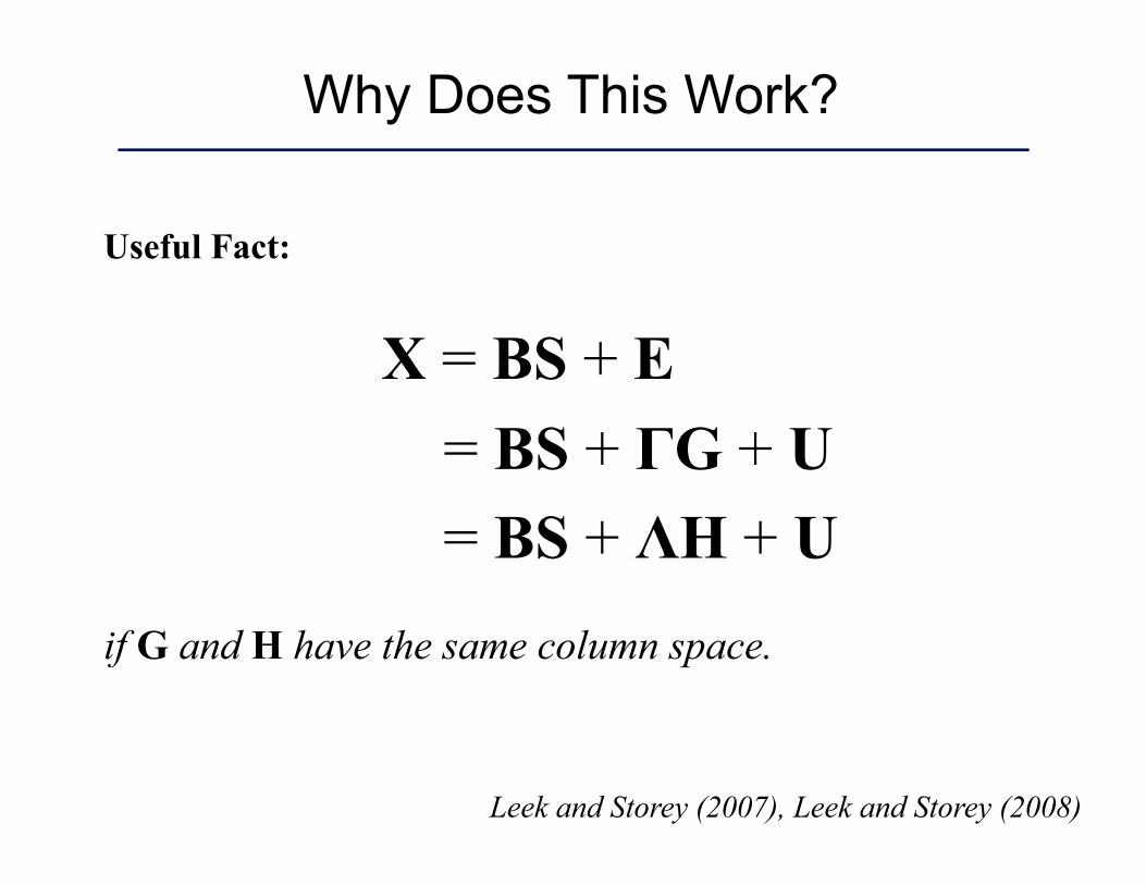
Why Does This Work?
Leek and Storey (2007), Leek and Storey (2008)
Useful Fact:
X = BS + E = BS + ΓG + U = BS + ΛH + U if G and H have the same column space.
• References:
Benjamini Y and Hochberg Y. (1995), “Controlling the false discovery rate – a practical and powerful approach to multiple testing.” JRSSB, 57: 289-300.
De Castro MC, Monte-Mor RL, Sawyer DO, and Singer, BH. (2005), “Malaria risk on the amazon frontier.” PNAS, 103: 2452-2457.
Delin B and Roeder K. (1999), “Genomic control for association studies.” Biometrics, 55: 997-1004.
Efron B. (2004) “Large-scale simultaneous hypothesis testing: The choice of a null hypothesis.” JASA, 99: 96-104.
Leek JT and Storey JD. (2008) “A general framework for multiple testing dependence.” Proceedings of the National Academy of Sciences , 105: 18718-18723.
Leek JT and Storey JD. (2007) “Capturing heterogeneity in gene expression studies by ‘Surrogate Variable Analysis’.” PLoS Genetics, 3: e161.
Taylor JE and Worsley KJ. (2007) “Detecting sparse signals in random fields, with applications to brain mapping.” JASA, 102: 913-928.
Thank You
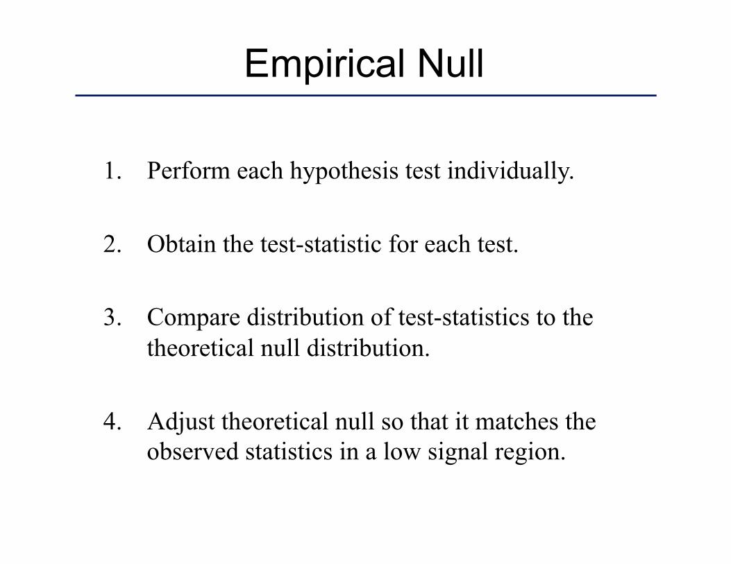
1. Perform each hypothesis test individually.
2. Obtain the test-statistic for each test.
3. Compare distribution of test-statistics to the theoretical null distribution.
4. Adjust theoretical null so that it matches the observed statistics in a low signal region.
Empirical Null
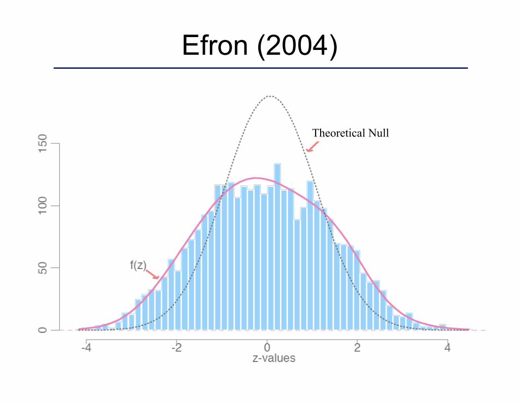
Theoretical Null
Efron (2004)
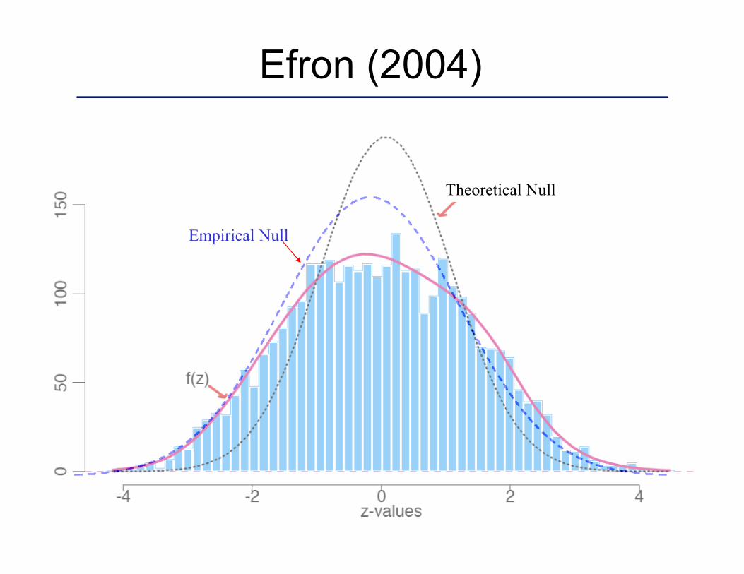
Theoretical Null
Empirical Null
Efron (2004)
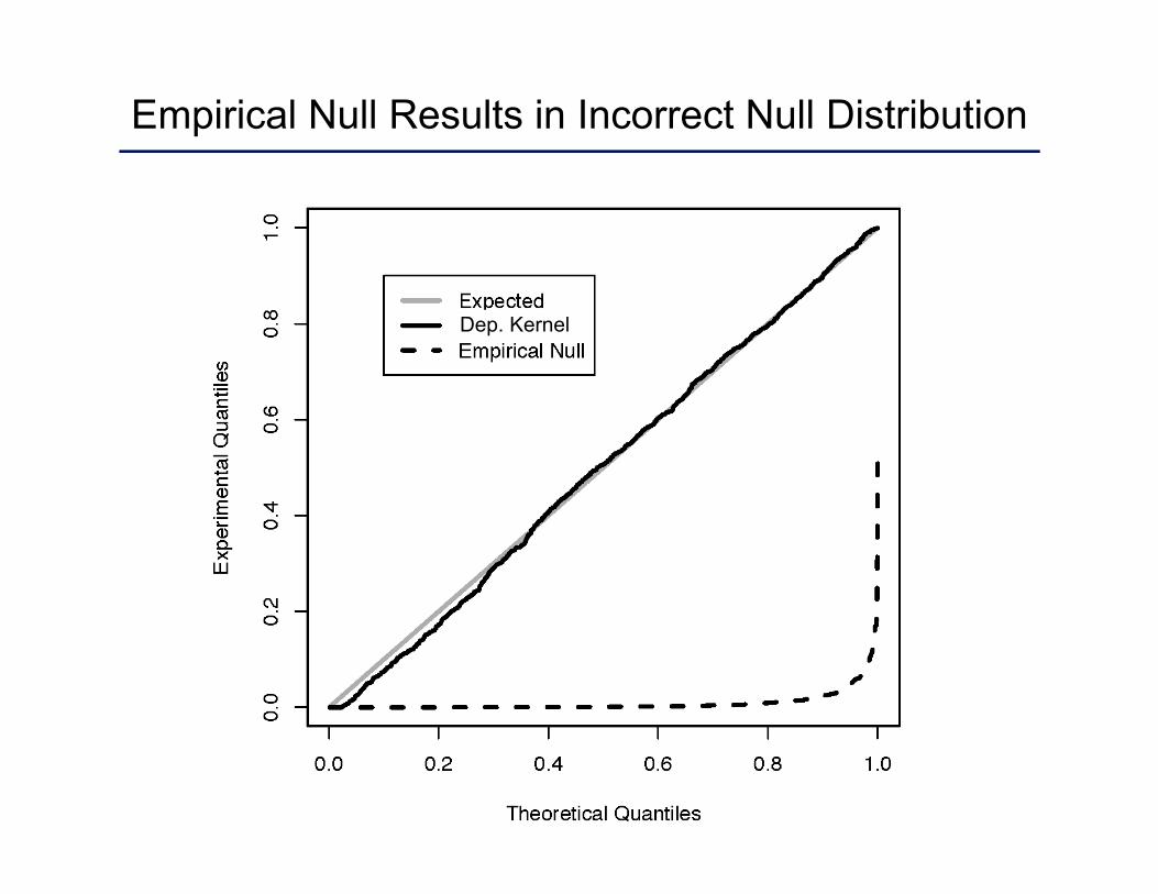
Empirical Null Results in Incorrect Null Distribution
Dep. Kernel
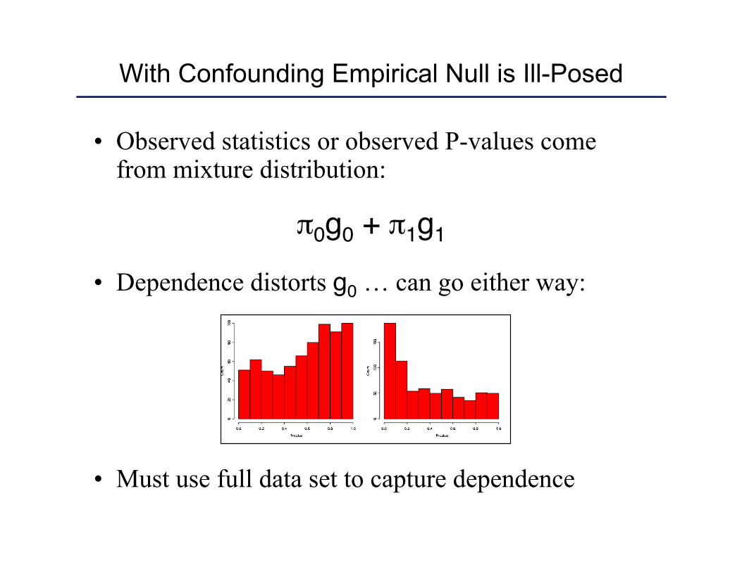
• Observed statistics or observed P-values come from mixture distribution:
π0g0 + π1g1
• Dependence distorts g0 … can go either way:
• Must use full data set to capture dependence
With Confounding Empirical Null is Ill-Posed