JAWS 2: Incident at Arched Rock

By Dave Cone Originally published in Bay Currents, Nov 1993

This time we can joke about it-nobody got hurt. For the second year in a row, autumn in Northern California was marked by a Great White Shark attack on a coastal kayaker.

Rosemary Johnson is a lifelong ocean sports enthusiast now living in Sonoma County. On Sunday October 10, she and three companions set off from Goat Rock Beach south of Jenner for the short paddle southward to Arched Rock (another Arch Rock lies north of Jenner). Rosemary was paddling a borrowed blue Frenzy, which is a plastic sit-on-top boat just nine feet long. Her friend Rick Larson, on his second kayak trip ever, was on a Scupper, and one of the others paddled a Kiwi, which is also a very short kayak.

As the four paddlers approached Arched Rock, Rosemary veered off from the group and headed around the rock. Rick and the others soon followed at some distance. Rosemary felt a powerful jolt and flew off the top of her boat. Rick saw a shark perhaps 16 feet long knock the boat entirely out of the water, and he believes Rosemary flew 12 to 14 feet into the air. Rosemary landed in the water, and briefly felt something solid underfoot. She thinks she landed on the shark. Wearing a wetsuit but no life vest, she had to swim in one direction to retrieve her paddle, then back the other way to get to her boat. She remained calm, believing that she had merely struck a rock.(!) Her approaching companions were less than calm, having seen the "monster" that hit her boat. Rick states that the shark's mouth encompassed almost the whole width of the Frenzy.

Rosemary hopped back on her kayak, but immediately capsized. She re-entered a second time and attempted to head toward shore, but had difficulty controlling the boat. When she capsized again, her friends saw the bite marks on her hull and realized that her boat was tippy and unmanageable because it was taking on water. They quickly improvised a rescue, with Rosemary riding belly down and head aft on the front of Rick's Scupper-"the only boat that could take me"-and the other paddlers towing the punctured boat. The group returned to the beach without further difficulty.

Back on dry land, the party reported the incident to Sonoma State Beaches rangers and inspected the boat. The damage measures 20 by 15 inches and lies entirely below the waterline approximately beneath the seat. A jagged crack runs perpendicular to the line of tooth marks. The pattern differs from the evidence left on Ken Kelton's boat, which shows tooth marks on both deck and hull (see "Ano Nuevo Revisited," Bay Currents, Dec. '92). Ken's shark held his boat for five to ten seconds, while Rosemary's contact was a collision rather than a grab-and-shake. Although it's common for sharks to intentionally release their prey after the initial attack, it is also possible that this shark simply bit more than it could chew, and Rosemary's boat popped out of it's maw like a watermelon seed between your fingers.

A researcher at Bodega Bay Marine Lab told the state park folks the size of the bite marks is consistent with a Great White up to 14 feet and 1500 pounds. Photos of the bite mark have been sent to shark expert Dr. Mark Marks at Humboldt State for more detailed analysis.

Park Rangers posted the beaches from Russian River to Bodega Head with shark warnings for five days after the attack, on the reasoning that Great Whites typically feed in an area for a few days and then move on. Of the numerous press accounts of the attack, the silliest was in the Santa Rosa Press-Democrat, which stated that "(Head Ranger Brian) Hickey said rangers don't know if the shark attacked on the first or last day it was in the Goat Rock area." Evidently the reporter was surprised that Hickey didn't have a copy of the shark's MISTIX reservation.

Rosemary and Rick visited the October 27 BASK general meeting, where Rosemary was peppered with questions, a few of them pertinent, and awarded a shark tee shirt and refrigerator magnet. Ken Kelton, BASK's own poster child for shark survival, greeted Rosemary, saying "You and I are members of a very exclusive club." Most of us are happy to see that club remain small.

How are such PREDICTIONS made?

HINT: Use your Trend Line

TASK #1 Unit 6 Math II - BEST MODELS How do these researchers determine the approximate size of the sharks based on the bite marks alone?

One measurement that is considered is the width of the mouth. First, researchers have to collect data on several sharks and then make a scatter plot. Use the data below to make a scatter plot.

Mouth Width (inches) 16" 18" 12" 17" 11" 15" 17" 16" 21"

Length of Shark (feet) 12.3' 16.2' 10.4' 13.6' 8.2' 11.7' 14.7' 13.6' 16.9'

1. Which variable above (Mouth Width or Shark Length) should be the independent variable (the input, x)? Why?

2. Which variable above (Mouth Width or Shark Length) should be the dependent variable (the output, y)? Why?

3. Make a SCATTER PLOT of the data at the right.

4. A trend line is a single straight line that best goes through the ‘center’ of all of the data points. (DO NOT JUST CONNECT THE POINTS) Draw a TREND LINE through the data points. (Using a piece of uncooked spaghetti works well to estimate placement.)

5. Using this trend line, we can now predict the size of a shark based on the

width of a shark's mouth. Give the approximate size of a shark that has a mouth width of 23".

6. Is your prediction in question #5 the exact same as everyone else in your class?

If it is NOT the same, whose prediction do you think is more accurate?

Who created a better trend line? Discuss.

7. What should be the properties of the BEST possible trend line using the given data? Discuss.

8. When 2 sets of data have a relatively linear relationship the data is either described as having a POSTIVE or NEGATIVE correlation. The data correlation is POSITIVE if both data sets move in the same direction (i.e. as one variable increases so does the other). The data correlation is NEGATIVE if the data sets move in opposite directions (i.e. as one variable increases the other decreases). What type of association does this data show?

23”

??

9. Most trend lines that are considered to be a “good fit” will be balanced such that the total RESIDUAL above and below the trend line is equal. RESIDUAL can be defined as the difference between the expected value and actual value (y). A more succinct definition, RESIDUAL can be described as the vertical distance (ොݕ)each data point is away from the trend line (with signed difference for above and below the trend line).

Find the RESIDUALs for each of the TREND LINES below (the SCATTER PLOT is the same in each graph).

10. What do all 4 trend lies above have in common? (optional: what is the approximate residual of your trend line from earlier)

11. To better analyze which trend line is best, it is common to consider comparing the sum of the squares of the residuals. Which trend line do you think is the best based on this new information? Is it the one you expected?

Data Point Residual

P1 1

P2 2

P3 –2

P4

P5

P6 Sum of

Residuals

Data Point Residual

P1

P2

P3

P4

P5

P6 Sum of

Residuals

Data Point Residual

P1

P2

P3

P4

P5

P6 Sum of

Residuals

Data Point Residual

P1

P2

P3

P4

P5

P6 Sum of

Residuals

TREND LINE 1 TREND LINE 2

TREND LINE 3 TREND LINE 4

-2

1

2

Data Point Residual Residual

Squared

P1 1 1

P2 2 4

P3 –2 4

P4

P5

P6

Sum

Data Point Residual Residual

Squared

P1

P2

P3

P4

P5

P6

Sum

Data Point Residual Residual

Squared

P1

P2

P3

P4

P5

P6

Sum

Data Point Residual Residual

Squared

P1

P2

P3

P4

P5

P6

Sum

TREND LINE 1 TREND LINE 2 TREND LINE 3 TREND LINE 4

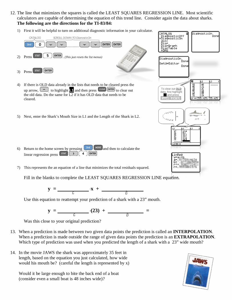
12. The line that minimizes the squares is called the LEAST SQUARES REGRESSION LINE. Most scientific calculators are capable of determining the equation of this trend line. Consider again the data about sharks. The following are the directions for the TI-83/84:

1) First it will be helpful to turn on additional diagnostic information in your calculator.

…….…

2) Press . (This just resets the list menus)

3) Press

4) If there is OLD data already in the lists that needs to be cleared press the up arrow, , to highlight L1 and then press to clear out the old data. Do the same for L2 if it has OLD data that needs to be cleared.

5) Next, enter the Shark’s Mouth Size in L1 and the Length of the Shark in L2.

6) Return to the home screen by pressing and then to calculate the linear regression press .

7) This represents the an equation of a line that minimizes the total residuals squared.

Fill in the blanks to complete the LEAST SQUARES REGRESSION LINE equation.

y = x +

Use this equation to reattempt your prediction of a shark with a 23” mouth.

y = (23) + =

Was this close to your original prediction?

13. When a prediction is made between two given data points the prediction is called an INTERPOLATION. When a prediction is made outside the range of given data points the prediction is an EXTRAPOLATION. Which type of prediction was used when you predicted the length of a shark with a 23” wide mouth?

14. In the movie JAWS the shark was approximately 35 feet in length, based on the equation you just calculated, how wide would his mouth be? (careful the length is represented by x)

Would it be large enough to bite the back end of a boat (consider even a small boat is 48 inches wide)?

CATALOG SCROLL DOWN TO DianosticOn

To clear out OLD data, first highlight

L1 and press CLEAR, ENTER.

a b

a b

15. A calculation called the correlation coefficient (r) is used to measure the extent to which the data for the two variables show a linear relationship. The closer the value is to 1 or –1 the stronger the linear relationship.

The formula for correlation coefficient is given by the equation:

y

i

x

i

syy

sxx

nr

11 , where

1 1,x y , 1 1,x y , …, 1 1,x y are the data points, x is the mean of the x-values, y is the mean of the y-values, xs is the standard deviation of the x-values, and ys is the standard deviation of the y-values. The TI-83/84 automatically calculates this result as long as the Diagnostic option is On. How strong of a linear relationship is shown by the data about sharks?

Matchbox Measures Task 1. Using a matchbox car and tracks, create a table of values and scatter

plot that shows the distance the car travels based on how high the starting ramp (as shown at in the diagrams at the right). Start with a single book to create the initial ramp and continue increasing so that you have at least 4 data points.

Determine which measure should be the independent and dependent variable. Create an appropriate scale for each of the axes.

0 Perfect Positive Linear

Relationship

No Linear

Relationship

Perfect Negative

Linear Relationship

Strong Weak None Strong Weak r:

Height of Ramp (cm)

Distance Traveled (cm)

2. Using your calculator, fill in the blanks to complete the LEAST SQUARES

REGRESSION LINE equation for the data collected with the match box car.

y = x +

3. How strong of a linear relationship is shown by the matchbox car data?

4. Using your LEAST SQUARES REGRESSIONS LINE, make a prediction how far the car will travel if the ramp is 9 cm. Is this an INTERPOLATION or an EXTAPOLATION?

= ( )+

Actually try releasing the car with the ramp at 9 cm high. How close was your prediction? Calculate the percent error (௧௨ ௨ିௗ௧ௗ ௨)

௧௨ ௨ .

5. How high would the ramp need to be for the car to travel a distance of 900 cm before coming to a rest? (Careful, you may need to solve for your solution).

= ( )+ Actually try releasing a car from the height you determined above. How many centimeters did your car get to 900 cm?

a b

a b

9cm

a b

COMPUTER COST The following show the value of a Pentium based computer system over a 7 year period.

Year 93' 94' 95' 96' 97' 98' 99'

value of computer

$3800 $3200 $2500 $2100 $1350 $900 $450

1. First determine an appropriate range and scale for the plot. 2. Make a Scatter Plot.

3. Draw a trend line 4. What type of association does the data show? 5. What is the correlation coefficient? 6. Estimate the cost of a Pentium computer in 1997.5 (interpolation or extrapolation) 7. Estimate the cost of a Pentium computer in 2009. (interpolation or extrapolation)

(careful this problem may suffer from the y2k bug) 8. Do you think the computer will ever be free? Explain your reasoning 9. Do you think the price will ever be negative? Is that possible? Explain. 10. Do you think there should be a domain restriction of the use of the trend lines (i.e.

just using the trend line for a limited number of years)?

LIP STICK CHARGE A company in California is test marketing a new line of lipsticks. The lipstick only costs the company $0.90 to make due to the volume production. The company located several different cities with approximately the same demographics and sold the exact same lipstick at different prices. They wanted to know which price would yield the largest profit. The following table shows the prices at which they were sold and the number sold at that price over a period of 3 months.

Cost $2.50 $4.00 $5.50 $7.00 $8.50 $10.00 Number

Sold 33 59 91 117 101 48

1. First determine an appropriate range and scale for the plot.

2. Make a Scatter Plot.

3. Draw a trend line or curve if more appropriate.

4. What type of association

does the data show? (Is it linear?) The TI-83/84 is capable of calculating quadratic, cubic, and quartic regression equations.

5. Explain why you think the data looks the way it does.

6. At what price do you think the company should charge to sell the most lipsticks?

7. At what price do you think they would make the largest profit?

8. Explain either why the prices you selected are the same in #6 and #7 or why they are different.

9. (OPTIONAL) Make a graph of the data on your calculator and on the grid.

i. Press

ii. If there is OLD data already in the lists that needs to be cleared press the up arrow, , to highlight L1 and then press to clear out the old data. Do the

same for L2 if it has OLD data that needs to be cleared. iii. Next, enter all of the Cost in L1 and the Number Sold in L2. iv. After entering the data, press and select all of the options shown

in the screen at the right. To do this move the cursor to the appropriate option ( ,

, )and press . To change the Xlist to L1 if needed move the cursor to Xlist and press and to the Ylist and press .

v. Finally, press . To make further adjustments to the graph window press . vi. Additionally, you can type the equation you calculated earlier in the to see the scatter plot and regression equation.

Enter the data from the chart into

L1 and L2

Select each of the following options by moving your

cursor to each and Pressing ENTER .

JUNK FOOD Calories and Fat Grams 1. The table displays data for Nutrition Guides of a single serving of particular foods. Find the equation of the best trend

line. What is your prediction as to how many Fat Grams a serving size of 200 Calories would have? a. What type of association does the data suggest? b. Create a scatter plot on the graph at the right and an

approximate trend line. c. Plot the data on the graph and using the TI-83/84. Then, find the

best possible line that fits the data using the TI-83/84's linear regression (4:linReg) command. What is the equation of the line?

y = .x + (a) (b) d. When a data point or two falls out of line from the rest of the data

that point is usually referred to as an outlier. Outliers can adversely affect the least squares regression line so that it doesn’t accurately represent the majority of the data (similar to how an outlier effects the mean). Would you describe any of the points in this set as an outlier?

e. When scatter plots contain outliers usually the median-median trend line is used instead of the least squares regression line (just as the medians are more resistant to the effects of outliers the median-median line is more resistant to outliers of a scatter plot). Calculate the median-median trend line. Calculating the equation of the median-median trend line requires that the data points are ordered from smallest to largest first coordinate and then separates the data into three equal, or nearly equal, groups with at least 1/3 of the data points in each of the first and last groups. The median x-values and y-values of each group are calculated. These medians, from smallest x-values to largest, are named 332211 ,,,,, yxyxyx . Then a line through the first and third medians is found. Finally, a line parallel to this line, 1/3 of the distance between the line and the remaining median is formed. The resulting line is of the following form

3

,, 321321

13

13 xxxayyybxxyyabaxy

. The TI83/84 is also capable of calculating this

trend line by selecting 3:Med-Med under the STAT menu. y = .x + (a) (b) f. Using each of your equations, predict the number of Fat Grams in an average serving of food that has

280 calories g. Is your prediction in problem #1c. an example of an

Food Pizza Rolls Pop Tarts Gold Fish Ck Kudo CC Dorritos Oreo Ice Cream Barron Pizza Toaster Strudel

Calories 230 220 150 130 140 160 340 190

Fat Grams 11 4 6 5 7 8 18 8

Interpolation OR Extrapolation Circle One

Prediction using Least Squares Line Prediction using Med-Med Line

Corvette Value

The table displays data for value of 1953 Corvette (EX122) in actual dollars over the years

a. Plot the data on the graph and using the TI-83. Then, find

the best possible line that fits the data using the TI-83's cubic regression (6:CubicReg) command. What is the equation of the line?

y = .x3 + .x2 + .x + . (a) (b) (c) (d)

b. Using your equation, what might be a good estimate for the value of the car in 2005?

and 2008?

c. Are your predictions in problem #2b. examples of an

d. In 2005, a 1953(EX122) of which only 300 were made sold on auction for $130,000 and in 2008, the model sold for $440,000. Were your cubic regression models still reasonable?

e. How well does the data fit a cubic equation? (Support your answer with the coefficient of determination)

Year 1953 (new) 1955 (used) 1960(used) 1963(used) 1968(used) 1970(used) 1975(used) 1978(used)

Value $3600 $2400 $1100 $1000 $3200 $4500 $7600 $18,500

Interpolation OR Extrapolation Circle One