Jaromír SkorkovskýKPH-ESF-MU Brno, Czech Republic

Brno, 2015

EOQ

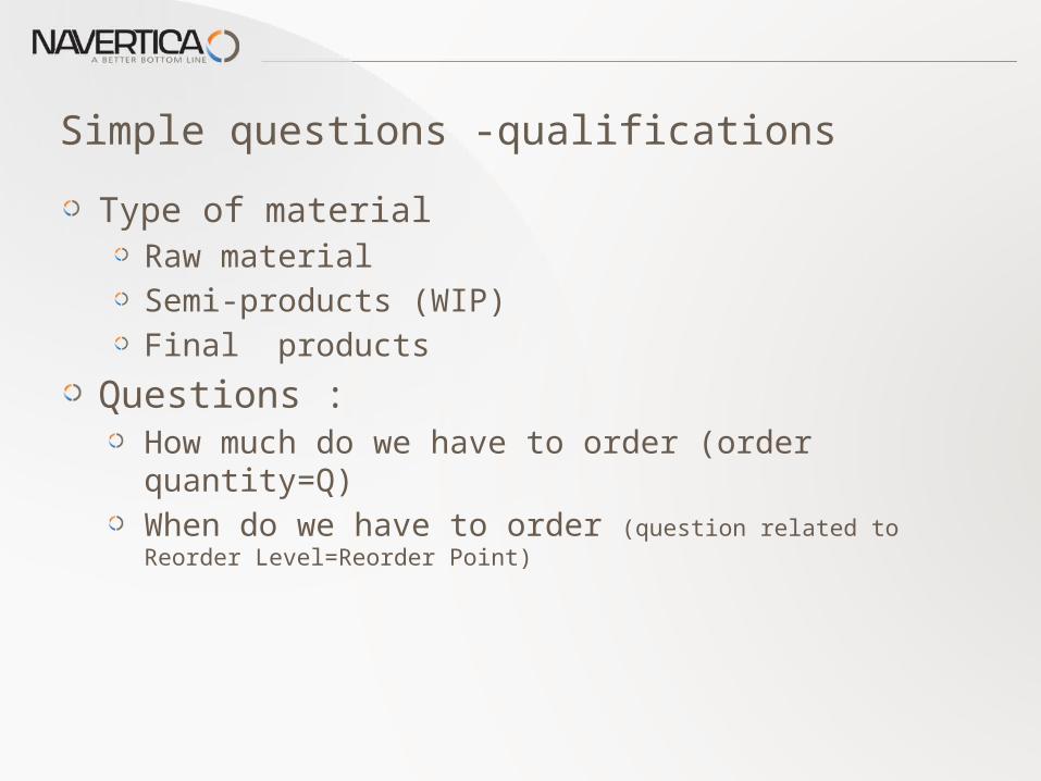
Type of materialRaw materialSemi-products (WIP)Final products

Questions :How much do we have to order (order quantity=Q)When do we have to order (question related to Reorder Level=Reorder Point)

Simple questions -qualifications

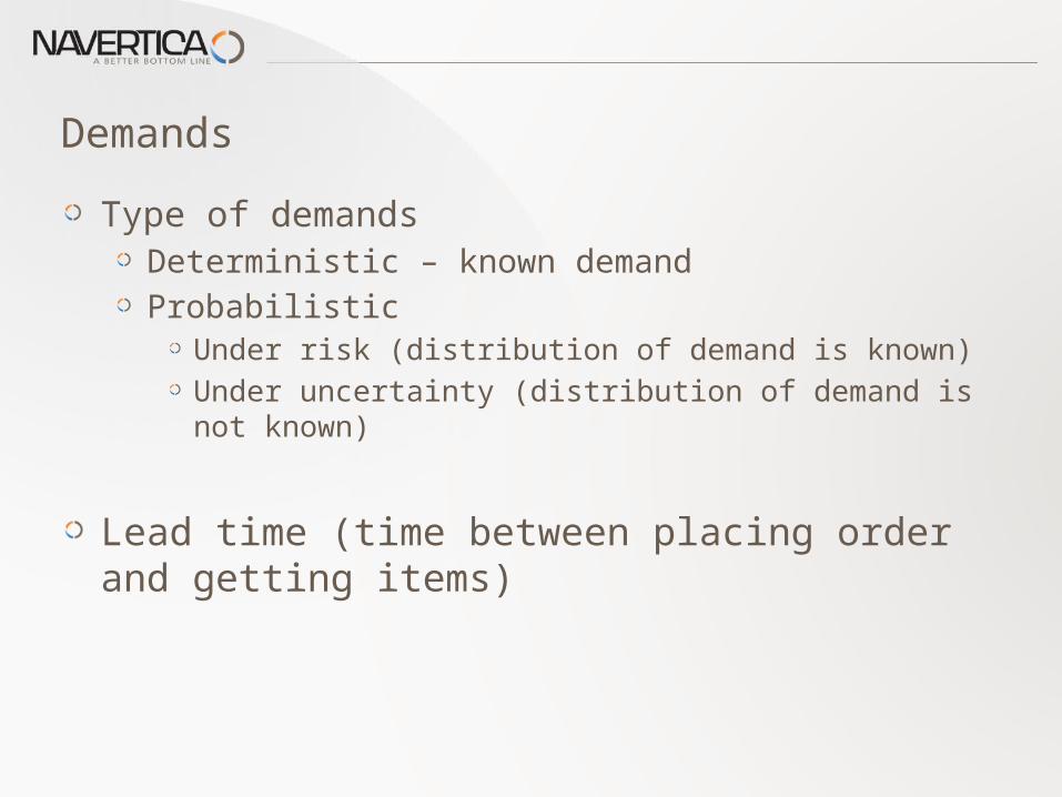
Type of demandsDeterministic – known demandProbabilistic

Under risk (distribution of demand is known)Under uncertainty (distribution of demand is not known)

Lead time (time between placing order and getting items)

Demands

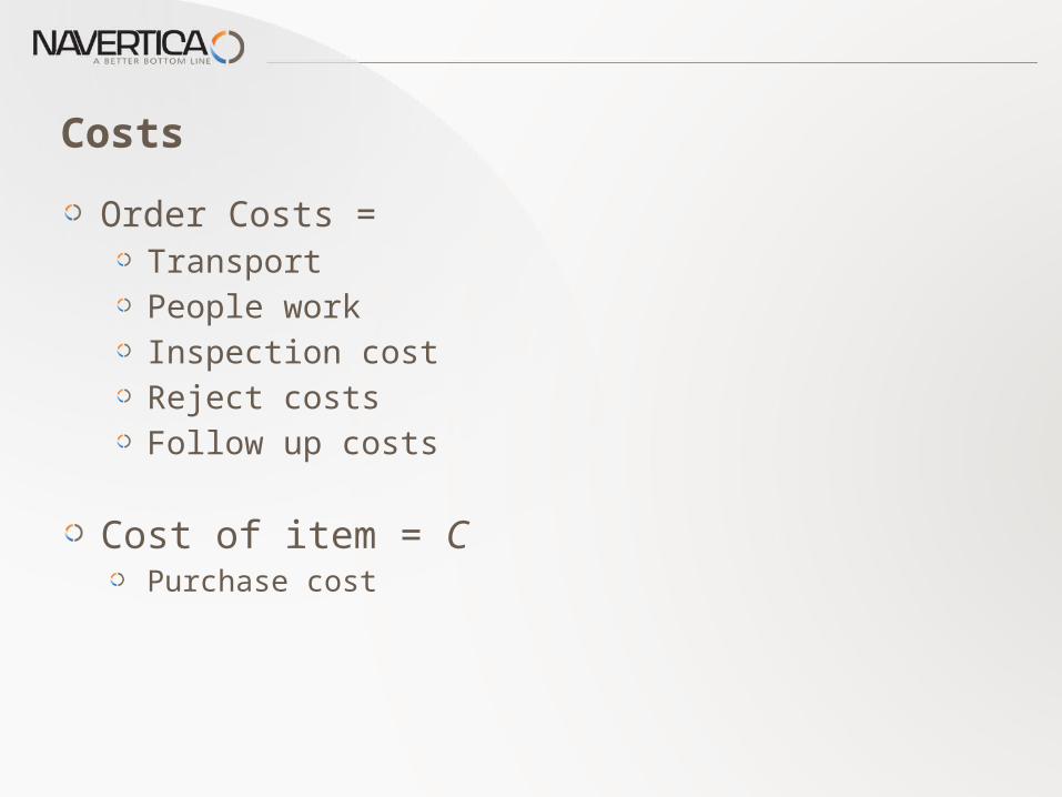
Order Costs = TransportPeople workInspection costReject costsFollow up costs

Cost of item = C

Purchase cost

Costs

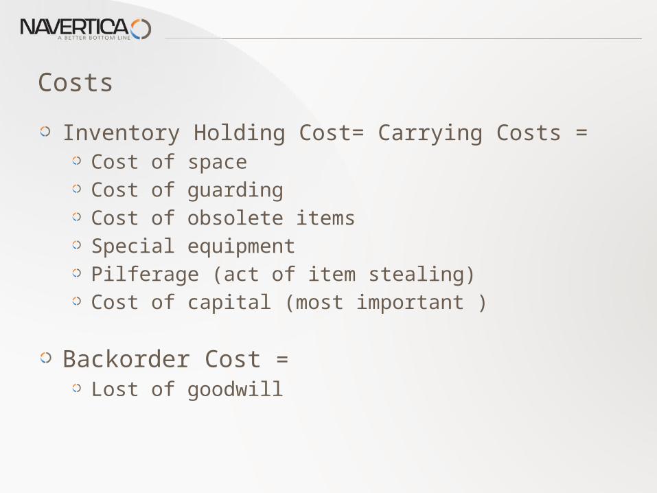
Inventory Holding Cost= Carrying Costs = Cost of spaceCost of guardingCost of obsolete itemsSpecial equipment Pilferage (act of item stealing)Cost of capital (most important )

Backorder Cost = Lost of goodwill

Costs

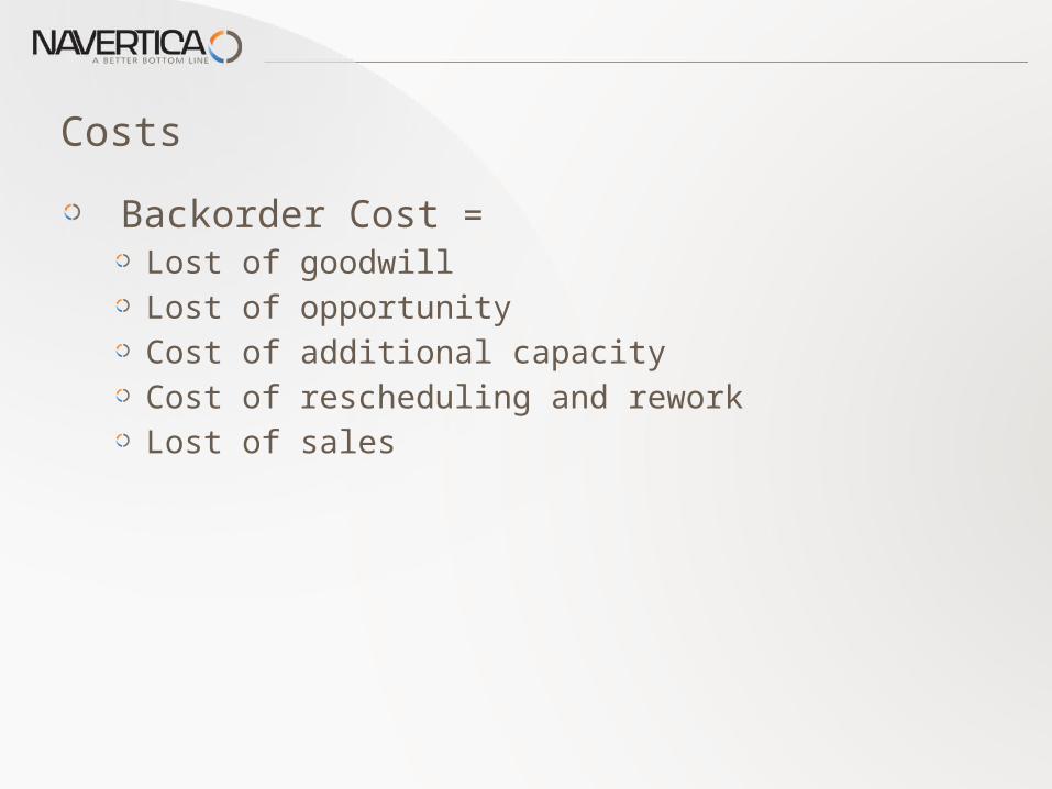
Backorder Cost = Lost of goodwill Lost of opportunityCost of additional capacityCost of rescheduling and reworkLost of sales

Costs

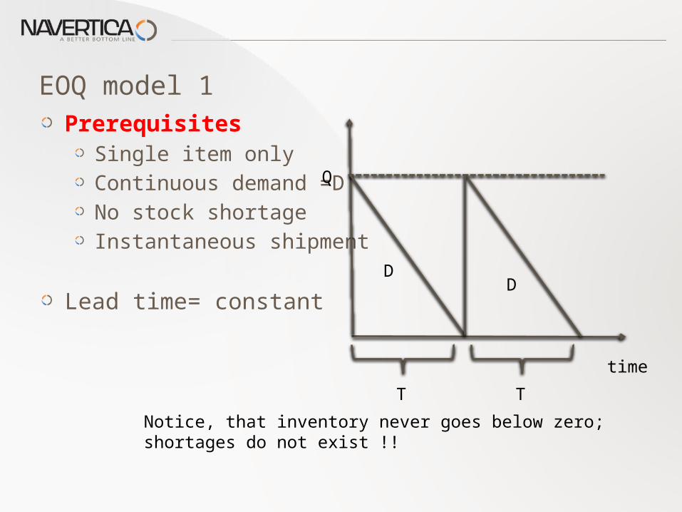
PrerequisitesSingle item onlyContinuous demand =DNo stock shortage Instantaneous shipment

Lead time= constant

EOQ model 1

D

Q

T

D

T

time

Notice, that inventory never goes below zero; shortages do not exist !!

8

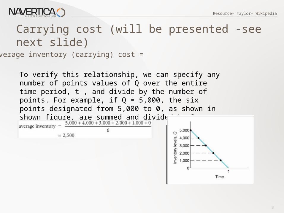
Carrying cost (will be presented -see next slide)

Resource- Taylor- Wikipedia

To verify this relationship, we can specify any number of points values of Q over the entire time period, t , and divide by the number of points. For example, if Q = 5,000, the six points designated from 5,000 to 0, as shown in shown figure, are summed and divided by 6:

Average inventory (carrying) cost =

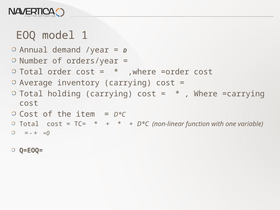
Annual demand /year = DNumber of orders/year = Total order cost = * ,where =order costAverage inventory (carrying) cost = Total holding (carrying) cost = * , Where =carrying costCost of the item = D*C Total cost = TC= * + * + D*C (non-linear function with one variable) = - + =0 Q=EOQ=

EOQ model 1

10

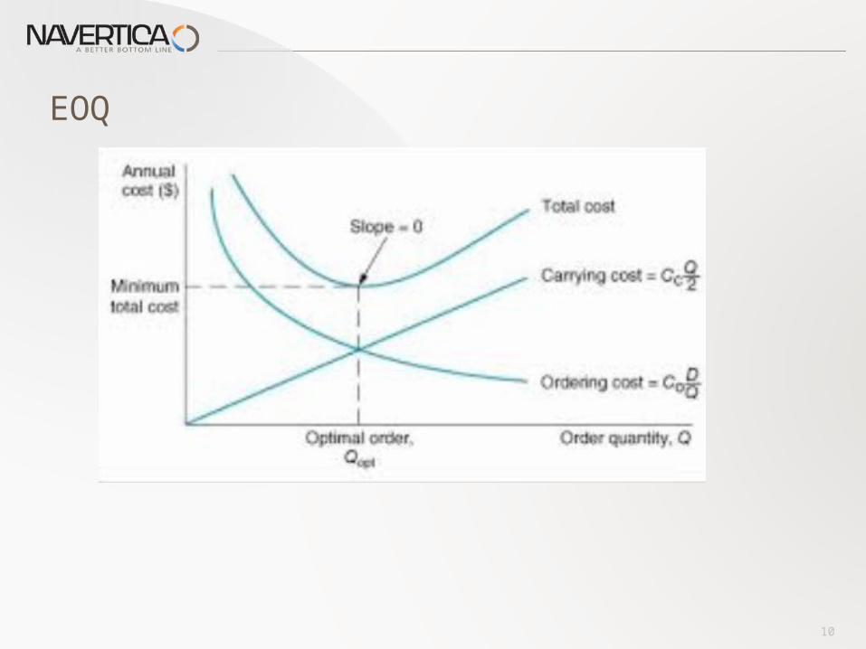
EOQ

Děkujeme za Vaši pozornost a čas