January 28, 2004Notes

– No office hour on Friday, Jan 30 (2–3), buttutorial from 1–2. (Check with 410.)

– Next Wednesday, Rafal Kustra will doSections 5.1–5.5

– Today we are doing 4.4, 4.3; that is all ofChapter 4

– The book ”Modern Applied Statistics withS” by Venables and Ripley is very useful. Makesure you have the MASS library available whenusing R or Splus (it is available on Cquest).All the code in the 3rd edition of the book isavailable in a file called ”scripts3”, in/u/radford/R-1.6.1/library/MASS.

1

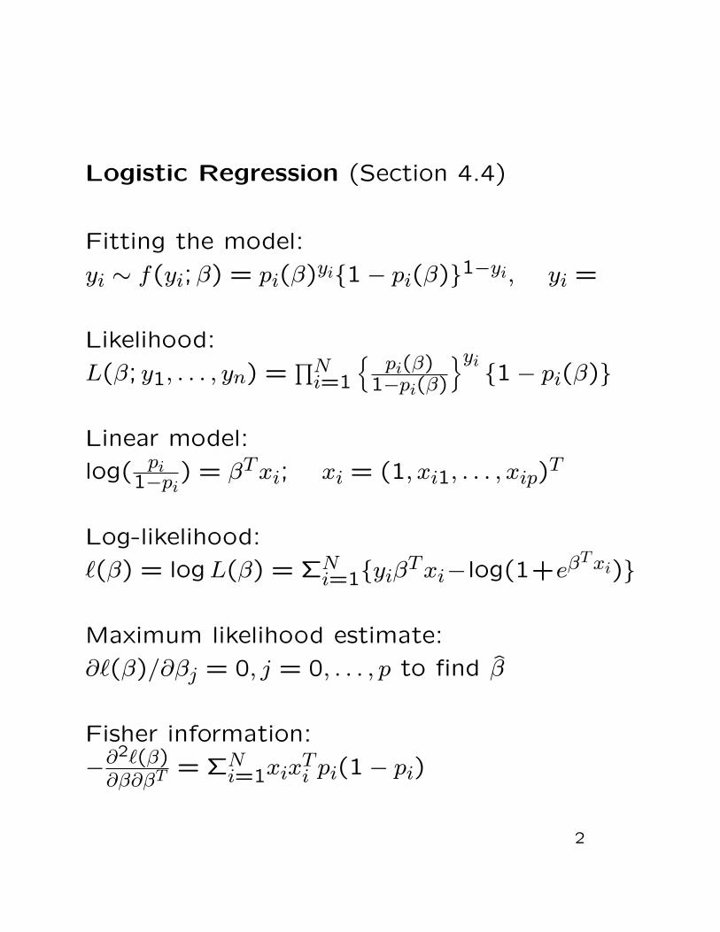
Logistic Regression (Section 4.4)

Fitting the model:

yi ∼ f(yi;β) = pi(β)yi{1− pi(β)}1−yi, yi =

Likelihood:

L(β; y1, . . . , yn) =∏N

i=1

{pi(β)

1−pi(β)

}yi {1− pi(β)}

Linear model:

log( pi1−pi

) = βTxi; xi = (1, xi1, . . . , xip)T

Log-likelihood:

`(β) = logL(β) = ΣNi=1{yiβ

Txi−log(1+eβT xi)}

Maximum likelihood estimate:

∂`(β)/∂βj = 0, j = 0, . . . , p to find β̂

Fisher information:

−∂2`(β)∂β∂βT = ΣN

i=1xixTi pi(1− pi)

2

Fitting: use an iteratively reweighted least squares

algorithm; equivalent to Newton-Raphson; p.99

Inference: β̂d→ N(β, {−`′′(β̂)}−1)

Component: β̂j ≈ N(βj, σ̂j) σ̂2j = [{−`′′(β̂)}−1]jj;

gives a t-test (z-test) for each component

2{`(β̂) − `(βj, β̃−j)} ≈ χ2dimβj

; in particular for

each component get a χ21, or equivalently

sign(β̂j − βj)√

[2{`(β̂)− `(βj, β̃−j)} ≈ N(0,1)

To compare 2 models M0 ⊂ M can use this

twice to get

2{`M(β̂) − `M0(β̃q)} ≈ χ2

p−q which provides a

test of the adequacy of M0

LHS is the difference in (residual) deviances;

analogous to SS in regression

3

– if yi ∼ Binom(ni, pi) same model applies

– E(yi) = pi, var(yi) = pi(1−pi) under Bernoulli,

– E(yi) = nipi and var(yi) = nipi(1− pi)under Binomial

– Often the model is generalized to allowvar(yi) = φpi(1− pi); called over-dispersion.

– Most software provides an estimate of φ basedon residuals.

– Model selection uses a Cp-like criterion calledAIC

– In Splus or R, use glm to fit logistic regres-sion, stepAIC for model selection

3-1

4

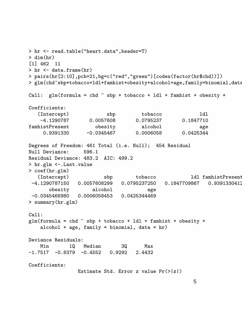
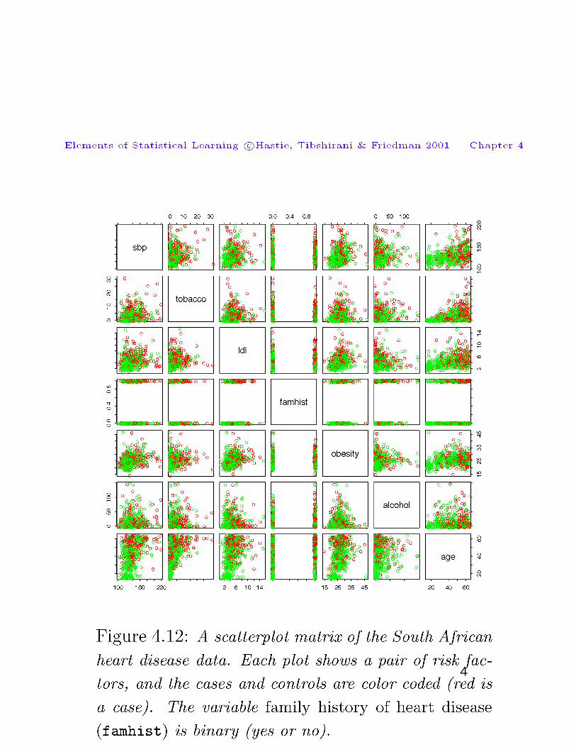
> hr <- read.table("heart.data",header=T)> dim(hr)[1] 462 11> hr <- data.frame(hr)> pairs(hr[2:10],pch=21,bg=c("red","green")[codes(factor(hr$chd))])> glm(chd~sbp+tobacco+ldl+famhist+obesity+alcohol+age,family=binomial,data=hr)

Call: glm(formula = chd ~ sbp + tobacco + ldl + famhist + obesity + alcohol + age, family = binomial, data = hr)

Coefficients:(Intercept) sbp tobacco ldl-4.1290787 0.0057608 0.0795237 0.1847710

famhistPresent obesity alcohol age0.9391330 -0.0345467 0.0006058 0.0425344

Degrees of Freedom: 461 Total (i.e. Null); 454 ResidualNull Deviance: 596.1Residual Deviance: 483.2 AIC: 499.2> hr.glm <-.Last.value> coef(hr.glm)

(Intercept) sbp tobacco ldl famhistPresent-4.1290787150 0.0057608299 0.0795237250 0.1847709867 0.9391330412

obesity alcohol age-0.0345466980 0.0006058453 0.0425344469

> summary(hr.glm)

Call:glm(formula = chd ~ sbp + tobacco + ldl + famhist + obesity +

alcohol + age, family = binomial, data = hr)

Deviance Residuals:Min 1Q Median 3Q Max

-1.7517 -0.8379 -0.4552 0.9292 2.4432

Coefficients:Estimate Std. Error z value Pr(>|z|)

5

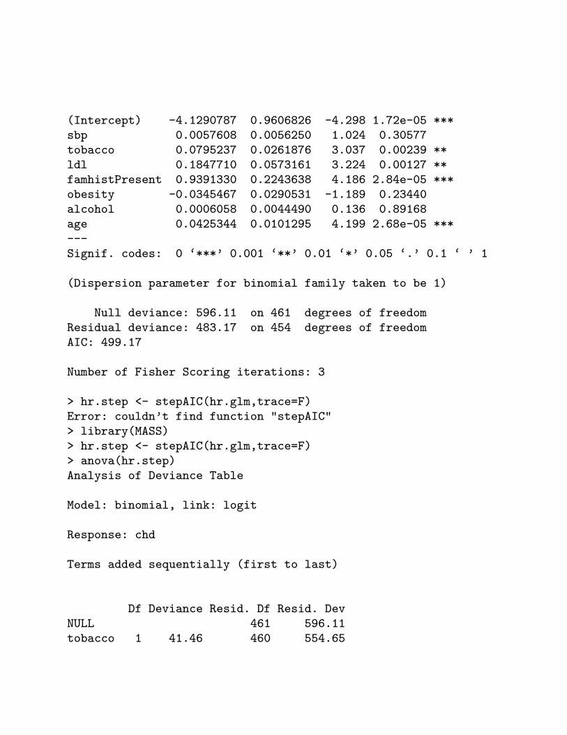
(Intercept) -4.1290787 0.9606826 -4.298 1.72e-05 ***sbp 0.0057608 0.0056250 1.024 0.30577tobacco 0.0795237 0.0261876 3.037 0.00239 **ldl 0.1847710 0.0573161 3.224 0.00127 **famhistPresent 0.9391330 0.2243638 4.186 2.84e-05 ***obesity -0.0345467 0.0290531 -1.189 0.23440alcohol 0.0006058 0.0044490 0.136 0.89168age 0.0425344 0.0101295 4.199 2.68e-05 ***---Signif. codes: 0 ‘***’ 0.001 ‘**’ 0.01 ‘*’ 0.05 ‘.’ 0.1 ‘ ’ 1

(Dispersion parameter for binomial family taken to be 1)

Null deviance: 596.11 on 461 degrees of freedomResidual deviance: 483.17 on 454 degrees of freedomAIC: 499.17

Number of Fisher Scoring iterations: 3

> hr.step <- stepAIC(hr.glm,trace=F)Error: couldn’t find function "stepAIC"> library(MASS)> hr.step <- stepAIC(hr.glm,trace=F)> anova(hr.step)Analysis of Deviance Table

Model: binomial, link: logit

Response: chd

Terms added sequentially (first to last)

Df Deviance Resid. Df Resid. DevNULL 461 596.11tobacco 1 41.46 460 554.65

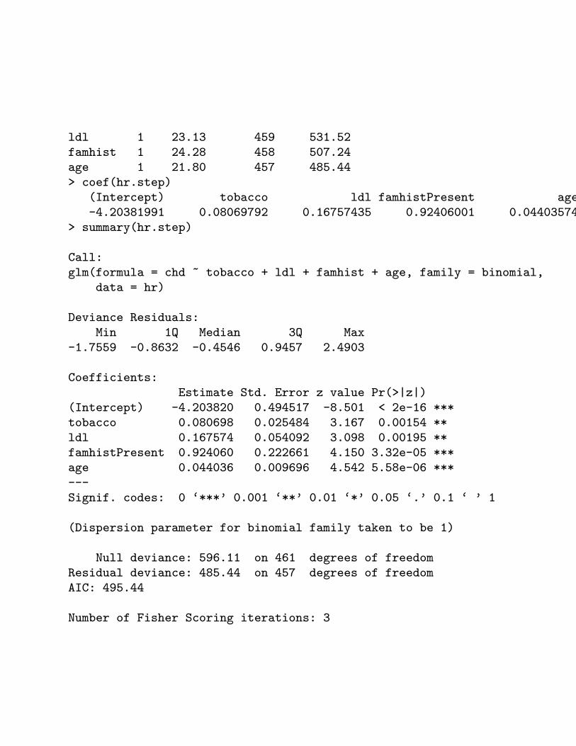
ldl 1 23.13 459 531.52famhist 1 24.28 458 507.24age 1 21.80 457 485.44> coef(hr.step)

(Intercept) tobacco ldl famhistPresent age-4.20381991 0.08069792 0.16757435 0.92406001 0.04403574

> summary(hr.step)

Call:glm(formula = chd ~ tobacco + ldl + famhist + age, family = binomial,

data = hr)

Deviance Residuals:Min 1Q Median 3Q Max

-1.7559 -0.8632 -0.4546 0.9457 2.4903

Coefficients:Estimate Std. Error z value Pr(>|z|)

(Intercept) -4.203820 0.494517 -8.501 < 2e-16 ***tobacco 0.080698 0.025484 3.167 0.00154 **ldl 0.167574 0.054092 3.098 0.00195 **famhistPresent 0.924060 0.222661 4.150 3.32e-05 ***age 0.044036 0.009696 4.542 5.58e-06 ***---Signif. codes: 0 ‘***’ 0.001 ‘**’ 0.01 ‘*’ 0.05 ‘.’ 0.1 ‘ ’ 1

(Dispersion parameter for binomial family taken to be 1)

Null deviance: 596.11 on 461 degrees of freedomResidual deviance: 485.44 on 457 degrees of freedomAIC: 495.44

Number of Fisher Scoring iterations: 3

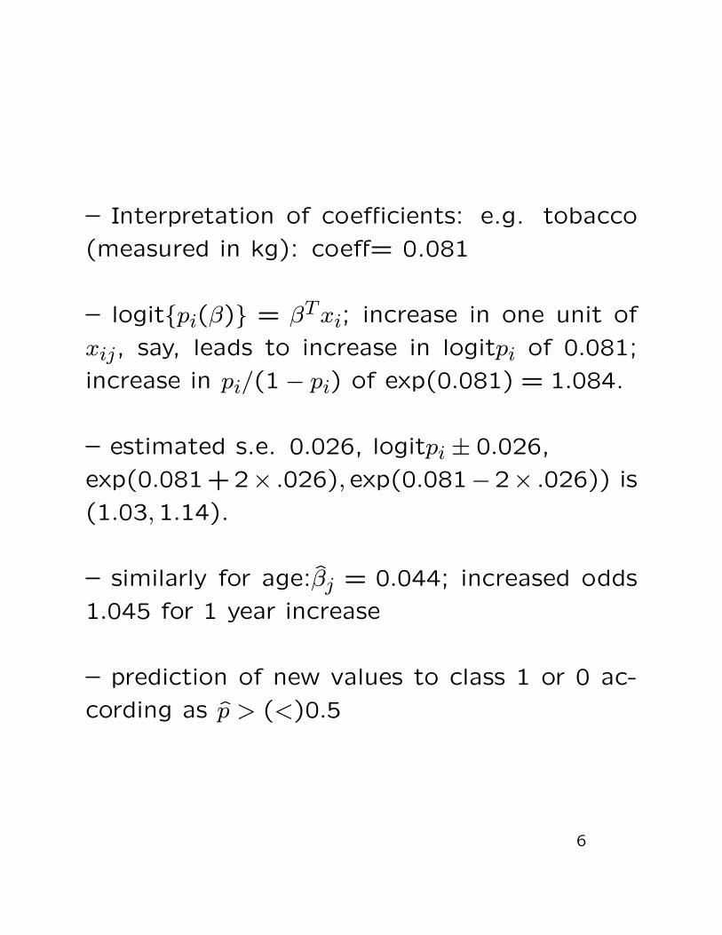
– Interpretation of coefficients: e.g. tobacco

(measured in kg): coeff= 0.081

– logit{pi(β)} = βTxi; increase in one unit of

xij, say, leads to increase in logitpi of 0.081;

increase in pi/(1− pi) of exp(0.081) = 1.084.

– estimated s.e. 0.026, logitpi ± 0.026,

exp(0.081+2× .026), exp(0.081−2× .026)) is

(1.03,1.14).

– similarly for age:β̂j = 0.044; increased odds

1.045 for 1 year increase

– prediction of new values to class 1 or 0 ac-

cording as p̂ > (<)0.5

6

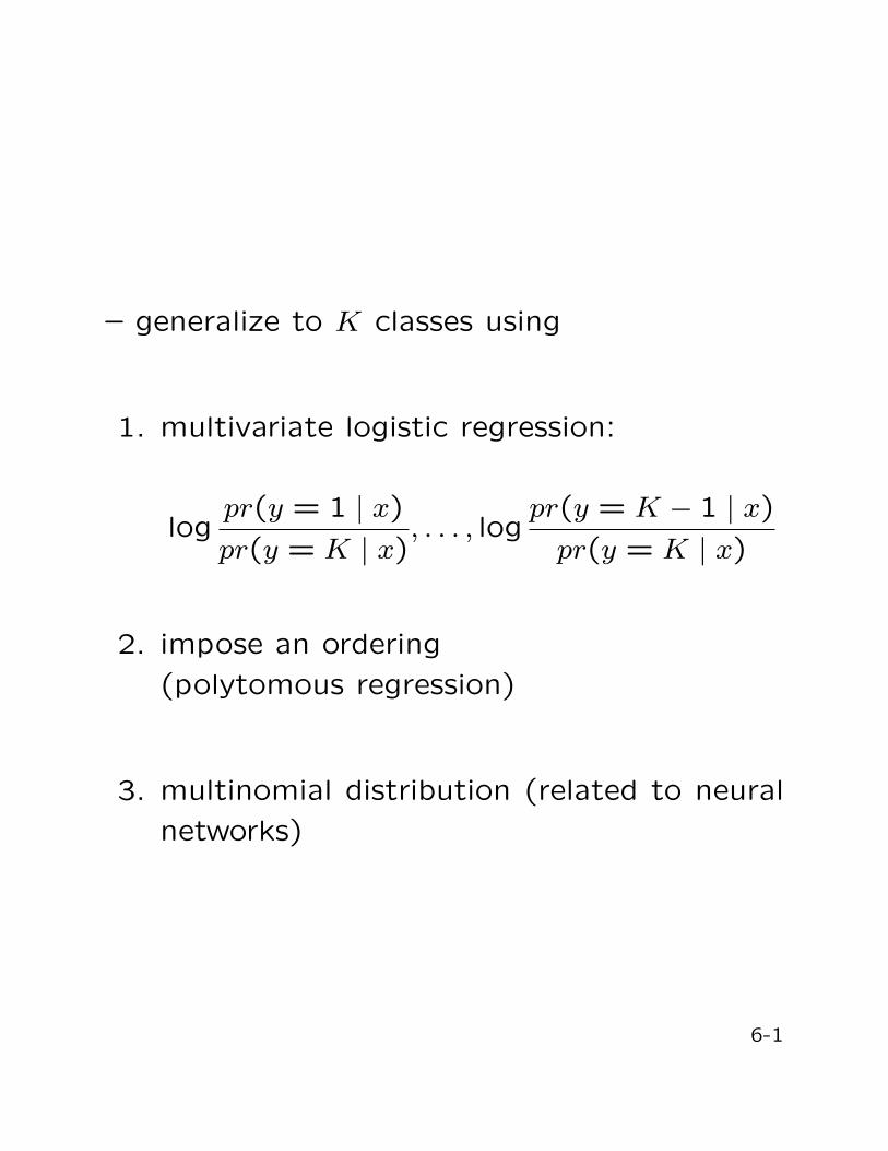
– generalize to K classes using

1. multivariate logistic regression:

logpr(y = 1 | x)pr(y = K | x)

, . . . , logpr(y = K − 1 | x)

pr(y = K | x)

2. impose an ordering

(polytomous regression)

3. multinomial distribution (related to neural

networks)

6-1

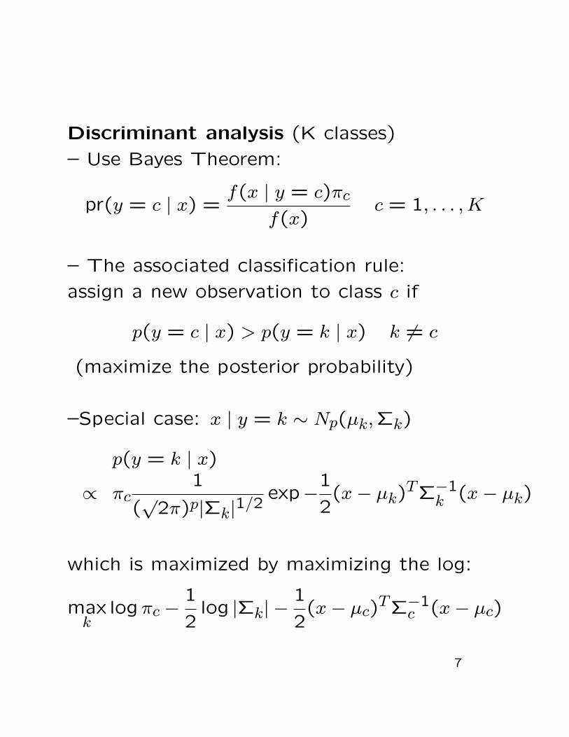
Discriminant analysis (K classes)

– Use Bayes Theorem:

pr(y = c | x) =f(x | y = c)πc

f(x)c = 1, . . . , K

– The associated classification rule:

assign a new observation to class c if

p(y = c | x) > p(y = k | x) k 6= c

(maximize the posterior probability)

–Special case: x | y = k ∼ Np(µk,Σk)

p(y = k | x)

∝ πc1

(√

2π)p|Σk|1/2exp−

1

2(x− µk)

TΣ−1k (x− µk)

which is maximized by maximizing the log:

maxk

logπc −1

2log |Σk| −

1

2(x− µc)

TΣ−1c (x− µc)

7

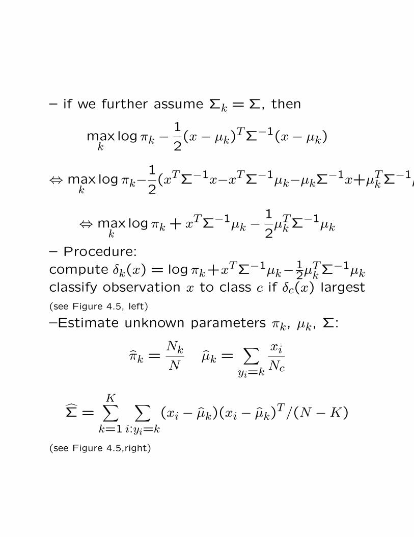
– if we further assume Σk = Σ, then

maxk

logπk −1

2(x− µk)

TΣ−1(x− µk)

⇔ maxk

logπk−1

2(xTΣ−1x−xTΣ−1µk−µkΣ

−1x+µTk Σ−1µk)

⇔ maxk

logπk + xTΣ−1µk −1

2µT

k Σ−1µk

– Procedure:compute δk(x) = logπk+xTΣ−1µk−1

2µTk Σ−1µk

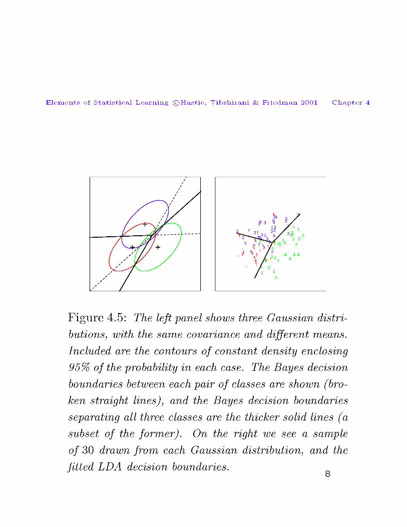
classify observation x to class c if δc(x) largest(see Figure 4.5, left)

–Estimate unknown parameters πk, µk, Σ:

π̂k =Nk

Nµ̂k =

∑yi=k

xi

Nc

Σ̂ =K∑

k=1

∑i:yi=k

(xi − µ̂k)(xi − µ̂k)T/(N −K)

(see Figure 4.5,right)

8

– Special case: 2 classes

– Choose class 2 if

log π̂2 + xT Σ̂−1µ̂2 − 12µ̂T

2 Σ̂−1µ̂2 >

log π̂1 + xT Σ̂−1µ̂1 − 12µ̂T

1 Σ̂−1µ̂1,

⇔ xT Σ̂−1(µ̂2 − µ̂1) >12(µ̂2Σ̂

−1µ̂2−12µ̂1Σ̂

−1µ̂1+log(N1/N)−log(N2/N)

– Note it is often common to specify πk = 1/K

in advance rather than estimating from the

data

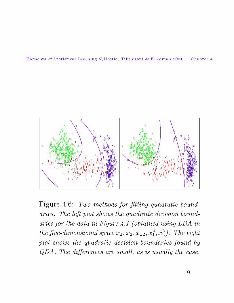
– If Σk not all equal, the discriminant func-

tion δk(x) defines a quadratic boundary; see

Figure 4.6, left

– An alternative is to augment the original set

of features with quadratic terms and use linear

discriminant functions; see Figure 4.6, right

8-1

9

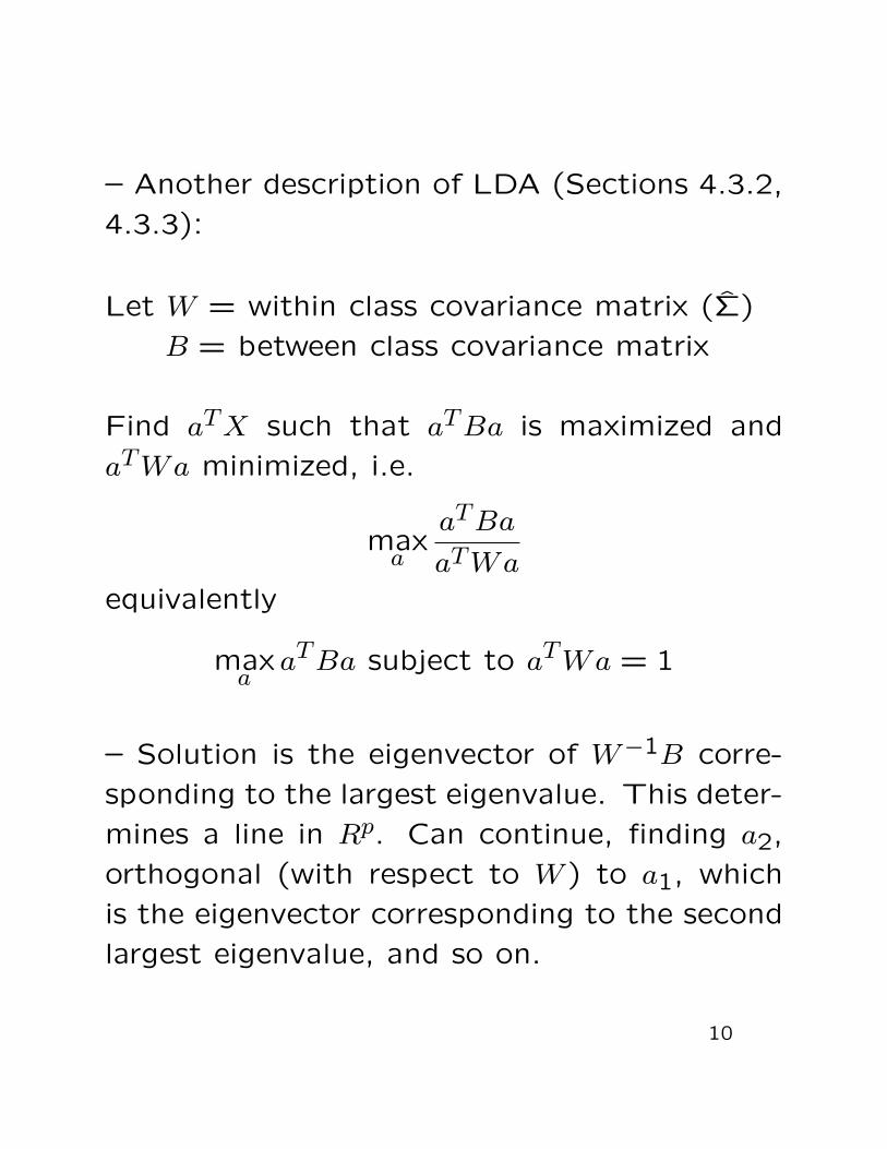
– Another description of LDA (Sections 4.3.2,

4.3.3):

Let W = within class covariance matrix (Σ̂)

B = between class covariance matrix

Find aTX such that aTBa is maximized and

aTWa minimized, i.e.

maxa

aTBa

aTWa

equivalently

maxa

aTBa subject to aTWa = 1

– Solution is the eigenvector of W−1B corre-

sponding to the largest eigenvalue. This deter-

mines a line in Rp. Can continue, finding a2,

orthogonal (with respect to W ) to a1, which

is the eigenvector corresponding to the second

largest eigenvalue, and so on.

10

There are at most min(p, K−1) positive eigen-

values.

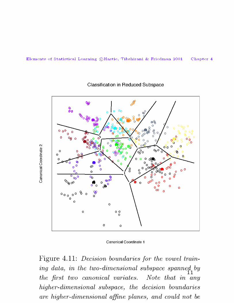
– These eigenvectors are the linear discrim-

inants, also called canonical variates. This

technique can be useful for visualization of the

groups. Figure 4.11 shows the 1st two canon-

ical variables for a data set with 10 classes.

11

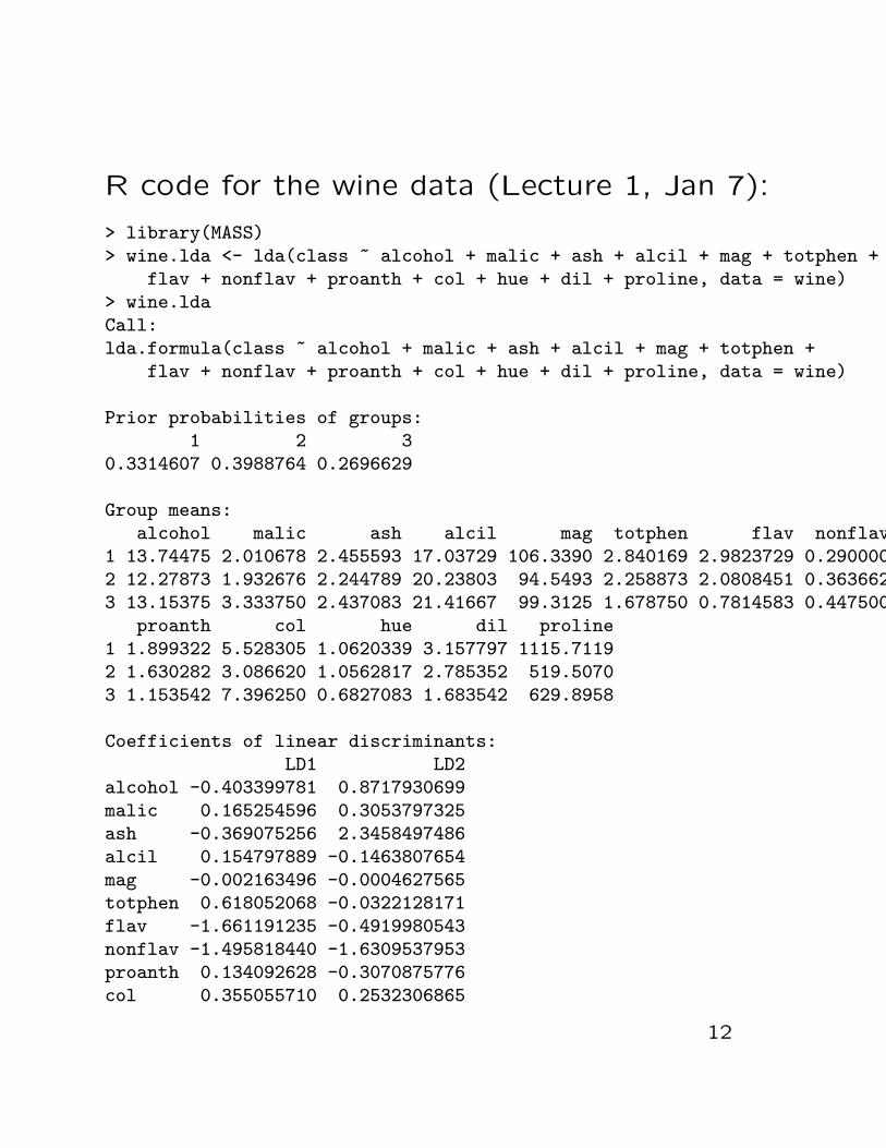
R code for the wine data (Lecture 1, Jan 7):

> library(MASS)> wine.lda <- lda(class ~ alcohol + malic + ash + alcil + mag + totphen +

flav + nonflav + proanth + col + hue + dil + proline, data = wine)> wine.ldaCall:lda.formula(class ~ alcohol + malic + ash + alcil + mag + totphen +

flav + nonflav + proanth + col + hue + dil + proline, data = wine)

Prior probabilities of groups:1 2 3

0.3314607 0.3988764 0.2696629

Group means:alcohol malic ash alcil mag totphen flav nonflav

1 13.74475 2.010678 2.455593 17.03729 106.3390 2.840169 2.9823729 0.2900002 12.27873 1.932676 2.244789 20.23803 94.5493 2.258873 2.0808451 0.3636623 13.15375 3.333750 2.437083 21.41667 99.3125 1.678750 0.7814583 0.447500

proanth col hue dil proline1 1.899322 5.528305 1.0620339 3.157797 1115.71192 1.630282 3.086620 1.0562817 2.785352 519.50703 1.153542 7.396250 0.6827083 1.683542 629.8958

Coefficients of linear discriminants:LD1 LD2

alcohol -0.403399781 0.8717930699malic 0.165254596 0.3053797325ash -0.369075256 2.3458497486alcil 0.154797889 -0.1463807654mag -0.002163496 -0.0004627565totphen 0.618052068 -0.0322128171flav -1.661191235 -0.4919980543nonflav -1.495818440 -1.6309537953proanth 0.134092628 -0.3070875776col 0.355055710 0.2532306865

12

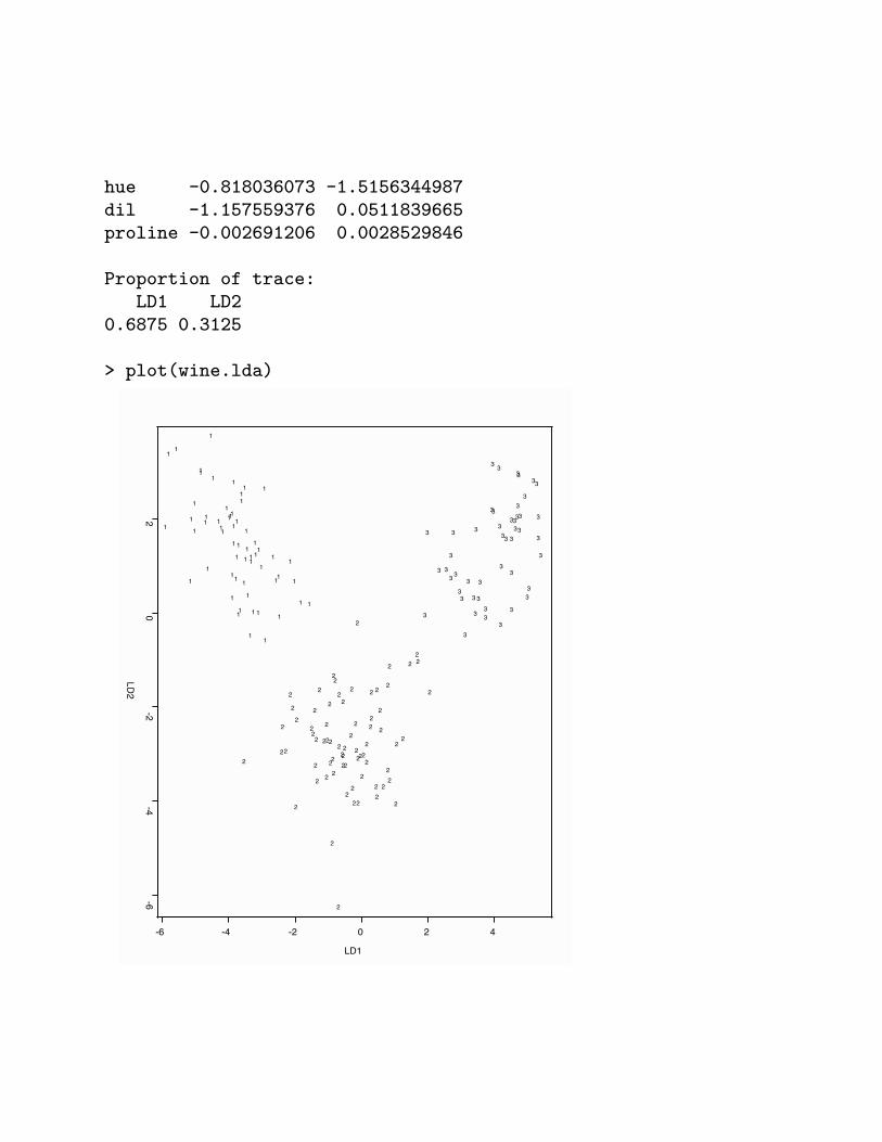
hue -0.818036073 -1.5156344987dil -1.157559376 0.0511839665proline -0.002691206 0.0028529846

Proportion of trace:LD1 LD2

0.6875 0.3125

> plot(wine.lda)

-6 -4 -2 0 2 4

-6-4

-20

2

LD1

LD2

1

1

1

1

1

111

1

1

1 111

1

11

1

1

1

1

11

1

11

1

11

1 1

1

1

11

1

1

1

1

1

1

1

1

1

1

1

1

1

1

1

1

11

1

1

1

1

11

2

2 2

2

2

2

2

22

2

2

2

2

2

2

2

2

2

2

2

2

2

2

2

2

2

2

22

2

2

2 2

2

2 2

2

2

2

2

2

2

2

2

2

2

2

2

2

2

2

2

2

2

2

2

2

22

2

2

2

2

2

2

2

2

2

2

2

2

3

3

3

3

3

3

3

3

3

3

3

3

33

3

3

3

33

33 3

3

3

3

3

3

3

3

3

3

3

3

3

3

3

3

33

3

3

3

33

3

3

3

3