Jansen KMC Introduction 2008
101
arXiv:cond-mat/0303028v1 [cond-mat.stat-mech] 3 Mar 2003 An Introduction To Monte Carlo Simulations Of Surface Reactions A. P. J. Jansen 1 February 2, 2008 1 e-mail: [email protected]
-
Upload
hkmydreams -
Category
Documents
-
view
233 -
download
1
Transcript of Jansen KMC Introduction 2008
arX
iv:c
ond-
mat
/030
3028
v1 [
cond
-mat
.sta
t-m
ech]
3 M
ar 2
003
An Introduction To Monte Carlo Simulations Of
Surface Reactions
A. P. J. Jansen1
February 2, 2008
1e-mail: [email protected]

ii
Contents
1 Introduction 1
2 A Stochastic Model for the Description of Surface Reaction Systems 32.1 The lattice gas . . . . . . . . . . . . . . . . . . . . . . . . . . . . . . . 3
2.1.1 Definitions . . . . . . . . . . . . . . . . . . . . . . . . . . . . . 42.1.2 Examples . . . . . . . . . . . . . . . . . . . . . . . . . . . . . . 42.1.3 Shortcomings . . . . . . . . . . . . . . . . . . . . . . . . . . . . 7
2.2 The Master Equation . . . . . . . . . . . . . . . . . . . . . . . . . . . . 82.2.1 Definition . . . . . . . . . . . . . . . . . . . . . . . . . . . . . . 82.2.2 Derivation . . . . . . . . . . . . . . . . . . . . . . . . . . . . . . 9
2.3 Working without a lattice . . . . . . . . . . . . . . . . . . . . . . . . . 13
3 How to Get the Transition Probabilities? 153.1 Quantum chemical calculations of transition probabilities . . . . . . . 153.2 Transition probabilities from experiments . . . . . . . . . . . . . . . . 21
3.2.1 Relating macroscopic properties to microscopic processes . . . 223.2.2 Unimolecular desorption . . . . . . . . . . . . . . . . . . . . . . 233.2.3 Unimolecular adsorption . . . . . . . . . . . . . . . . . . . . . . 253.2.4 Unimolecular reactions . . . . . . . . . . . . . . . . . . . . . . . 263.2.5 Diffusion . . . . . . . . . . . . . . . . . . . . . . . . . . . . . . 273.2.6 Bimolecular reactions . . . . . . . . . . . . . . . . . . . . . . . 273.2.7 Bimolecular adsorption . . . . . . . . . . . . . . . . . . . . . . 30
4 Monte Carlo Simulations 334.1 Solving the Master Equation . . . . . . . . . . . . . . . . . . . . . . . 33
4.1.1 The integral formulation of the Master Equation. . . . . . . . . 334.1.2 The Variable Step Size Method. . . . . . . . . . . . . . . . . . 344.1.3 Enabled and disabled reactions. . . . . . . . . . . . . . . . . . . 364.1.4 Weighted and uniform selection. . . . . . . . . . . . . . . . . . 384.1.5 Handling disabled reactions. . . . . . . . . . . . . . . . . . . . . 394.1.6 Reducing memory requirements. . . . . . . . . . . . . . . . . . 414.1.7 Oversampling and the Random Selection Method. . . . . . . . 424.1.8 The First Reaction Method. . . . . . . . . . . . . . . . . . . . . 444.1.9 Practical considerations . . . . . . . . . . . . . . . . . . . . . . 464.1.10 Time-dependent transition probabilities. . . . . . . . . . . . . . 48
4.2 A comparison with other methods. . . . . . . . . . . . . . . . . . . . . 504.2.1 The fixed time step method . . . . . . . . . . . . . . . . . . . . 50
iii
iv CONTENTS
4.2.2 Algorithmic approach . . . . . . . . . . . . . . . . . . . . . . . 504.2.3 Kinetic Monte Carlo . . . . . . . . . . . . . . . . . . . . . . . . 514.2.4 Cellular Automata . . . . . . . . . . . . . . . . . . . . . . . . . 52
4.3 The CARLOS program . . . . . . . . . . . . . . . . . . . . . . . . . . 524.4 Dynamic Monte Carlo simulations of rate equations . . . . . . . . . . 55
5 Modeling Reaction Systems 595.1 Unimolecular adsorption, . . . . . . . . . . . . . . . . . . . . . . . . . . 595.2 Bimolecular reactions . . . . . . . . . . . . . . . . . . . . . . . . . . . 605.3 Multiple sites . . . . . . . . . . . . . . . . . . . . . . . . . . . . . . . . 645.4 Systems without translational symmetry . . . . . . . . . . . . . . . . . 675.5 Infinitely fast reactions . . . . . . . . . . . . . . . . . . . . . . . . . . . 695.6 Diffusion . . . . . . . . . . . . . . . . . . . . . . . . . . . . . . . . . . . 725.7 Lateral interactions . . . . . . . . . . . . . . . . . . . . . . . . . . . . . 74
6 Examples 796.1 The Ziff-Gulari-Barshad model . . . . . . . . . . . . . . . . . . . . . . 796.2 TPD/TPR of 2AB → A2 + B2 . . . . . . . . . . . . . . . . . . . . . . 826.3 TPD with strong repulsive interactions . . . . . . . . . . . . . . . . . . 836.4 CO electrooxidation on a Pt-Ru electrode . . . . . . . . . . . . . . . . 856.5 Oscillations of CO oxidation on Pt surfaces . . . . . . . . . . . . . . . 87
Chapter 1
Introduction
If one is used to looking at chemical processes from an atomic point of view, then thefield of chemical kinetics is very complicated. Kinetics is generally studied on meso-or macroscopic scales. Atomic scales are of the order of Angstrøm and femtoseconds.Typical length scales in laboratory experiments vary between micrometers to cen-timeters, and typical time scales are often of the order of seconds or longer. Thismeans that there many orders of difference in length and time between the individualreactions and the resulting kinetics.
The length gap is not always a problem. Many systems are homogeneous, andthe kinetics of a macroscopic system can be reduced to the kinetics of a few reactingmolecules. This is generally the case for reactions in the gas phase and in solutions.For reactions on the surface of a catalyst it is not clear when this is the case. Itis certainly the case that in the overwhelming number of studies on the kinetics inheterogeneous catalysis it is implicitly assumed that the adsorbates are well-mixed,and that macroscopic rate equations can be used. These equations have the form
dθA
dt= −k
(1)A θA +
∑
B6=A
k(1)B θB (1.1)
−2k(2)A θ2
A −∑
B6=A
k(2)ABθAθB +
∑
B,C6=A
k(2)BCθBθC + . . .
with θA the so-called coverage of adsorbate A, which is the number of A’s per unit areaof the surface on which the reactions take place. The terms stand for the reactionsA → . . ., B → A, 2A → . . ., A + B → . . ., and B + C → A, respectively. The k’s arerate constants. If a position dependence θ = θ(r, t) is included we also need a diffusionterm. The result is called a reaction-diffusion equation. Simulations of reactions onsurfaces and detailed studies in surface science over the last few years have shown thatthe macroscopic rate equations are only rarely correct. Moreover, there are systemsthat show the formation of patterns with a characteristic length scale of micro- tocentimeters. For such systems it is not clear at all what the relation is between themacroscopic kinetics and the individual reactions.
Even more of a problem is the time gap. The typical atomic time scale is givenby the period of a molecular vibration. The fastest vibrations have a reciprocalwavelength of up to 4000 cm−1, and a period of about 8.3 fs. Reactions in catalysistake place in seconds or more. It is important to be aware of the origin of these
1
2 Chapter 1. Introduction
fifteen orders of magnitude difference. A reaction can be regarded as a movementof the system from one local minimum on a potential-energy surface to another. Insuch a move a so-called activation barrier has to be overcome. Most of the time thesystem moves around one local minimum. This movement is fast, in the order offemtoseconds, and corresponds to a superposition of all possible vibrations. Everytime that the system moves in the direction of the activation barrier can be regardedas an attempt to react. The probability that the reaction actually succeeds can beestimated by calculating a Boltzmann factor that gives the relative probability offinding the system at a local minimum or on top of the activation barrier. ThisBoltzmann factor is given by exp[−Ebar/RT ], where Ebar is the height of the barrier,R is the gas constant, and T is the temperature. A barrier of Ebar = 100 kJ/molat room temperature gives a Boltzmann factor of about 10−18. Hence we see thatthe very large difference in time scales is due to the very small probability that thesystem overcomes activations barriers.
In Molecular Dynamics a reaction with a high activation barrier is called a rareevent, and various techniques have been developed to get a reaction even when astandard simulation would never show it. These techniques, however, work for onereacting molecule or two molecules that react together, but not when one is inter-ested in the combination of thousands or more reacting molecules that one has whenstudying kinetics. The purpose of this course is to show how one deals with such acollection of reacting molecules. It turns out that one has to sacrifices some of thedetailed information that one has in Molecular Dynamics simulations. One can stillwork on atomic length scales, but one cannot work with the exact position of all atomsin a system. Instead one only specifies near which minimum of the potential-energysurface the system is. One does not work with the atomic time scale. Instead onehas the reactions as elementary events: i.e., one specifies at which moment the sys-tem moves from one minimum of the potential-energy surface to another. Moreover,because one doesn’t know where the atoms are exactly and how they are moving,one cannot determine the times for the reactions exactly either. Instead one canonly give probabilities for the times of the reactions. It turns out, however, that thisinformation is more than sufficient for studying kinetics.
Chapter 2
A Stochastic Model for theDescription of SurfaceReaction Systems
2.1 The lattice gas
The size of the time step, and with this computational cost, in simulations of the mo-tion of atoms and molecules is determined by the fast vibrations of chemical bonds.[1]Because the activation energies of chemical reactions are generally much higher thanthe thermal energies, chemical reactions take place on a time scale that is many ordersof magnitude larger. If one wants to study the kinetics on surfaces, then one needs amethod that does away with the fast motions.
The method that we present here does this by using the concept of sites. The forcesworking on an atom or a molecule that adsorbs on the catalyst force it to well-definedpositions on the surface.[2, 3] These positions are called sites. They correspond tominima on the potential-energy surface for the adsorbate. Most of the time adsorbatesstay very near these minima. Only when they diffuse from one site to another orduring a reaction they will not be near a minima for a very short time. Instead ofspecifying the precise positions, orientations, and configurations of the adsorbates wewill only specify for each sites its occupancy. A reaction and a diffusion from onesite to another will be modeled as a sudden change in the occupancy of the sites.Because the elementary events are now the reactions and the diffusion, the time thata system can be simulated is no longer determined by fast motions of the adsorbates.By taking a slightly larger length scale, we can simulate a much longer time scale.
If the surface of the catalyst has two-dimensional translational symmetry, or whenit can be modeled as such, the sites form a regular grid or a lattice. Our model isthen a so-called lattice-gas model. This chapter shows how this model can be used todescribe a large variety of problems in the kinetics of surface reactions.
3
4 Chapter 2. A Stochastic Model for the Description of Surface Reaction Systems
2.1.1 Definitions
If the catalyst has two-dimensional translational symmetry then there are two vectors,a1 and a2, with the property that when the catalyst is translated over any of thesevectors the result is indistinguishable from the situation before the translation. It issaid that the system is invariant under translation over these vectors. The vectors a1
and a2 are called primitive vectors . In fact the catalyst is invariant under translationalfor any vector of the form
x = n1a1 + n2a2 (2.1)
where n1 and n2 are integers. These vectors are the lattice vectors . The primitivevectors a1 and a2 are not uniquely defined. For example a (111) surface of a fcc metalis translationally invariant for a1 = a(1, 0) and a2 = a(1/2,
√3/2), where a is the
lattice spacing. But one can just as well choose a1 = a(1, 0) and a2 = a(−1/2,√
3/2).The area defined by
x = x1a1 + x2a2 (2.2)
with x1, x2 ∈ [0, 1〉 is called the unit cell . The whole system is retained by tiling theplane with the contents of a unit cell.
Expression (2.1) defines a simple lattice, Bravais lattice, or net . Simple latticeshave just one lattice point, or grid point, per unit cell. It is also possible to have morethan one lattice point per unit cell. The lattice is then given by all
x = x(i)0 + n1a1 + n2a2 (2.3)
with i = 0, 1, . . . , Nsub − 1. Each x(i)0 is a different vectors in the unit cell. The
set x(i)0 + n1a1 + n2a2 for a particular vector i forms a sublattice, which is itself
a simple lattice. There are Nsub sublattices, and they are all equivalent; they areonly translated with respect to each other. (For more information on lattices see forexample references [4] and [2]).
We assign a label to each lattice point. The lattice points correspond to thesites, and the labels specify properties of the sites. The most common property thatone wants to describe with the label is the occupancy of the site. For example, theshort-hand notation (n1, n2/s : A) can be interpreted as that the site at position
x(s)0 + n1a1 + n2a2 is occupied by a molecule A. The labels can also be used the
specify reactions. A reaction is nothing but a change in the labels. An extensionof the short-hand notation (n1, n2/s : A → B) indicates that during a reaction the
occupancy of the site at x(s)0 + n1a1 + n2a2 changes from A to B. If more than one
site is involved in a reaction then the specification will consist of a set changes of theform (n1, n2/s : A → B).
2.1.2 Examples
Figure 2.1 shows a Pt(111) surface. CO prefers to adsorb on this surface at thetop sites.[2] We can therefore model CO on this surface with a simple lattice withthe lattice points corresponding to the top sites. We have a1 = a(1, 0) and a2 =
a(1/2,√
3/2). As Nsub = 1 we choose x(0)0 = (0, 0) for simplicity. Each grid point has
a label that we choose to be equal to CO or ∗. The former indicates that the site isoccupied by a CO molecule, the latter that the site is vacant.
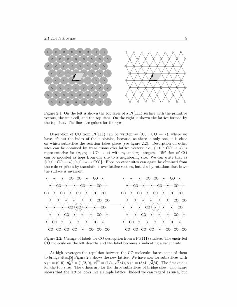
2.1 The lattice gas 5
Figure 2.1: On the left is shown the top layer of a Pt(111) surface with the primitivevectors, the unit cell, and the top sites. On the right is shown the lattice formed bythe top sites. The lines are guides for the eyes.
Desorption of CO from Pt(111) can be written as (0, 0 : CO → ∗), where wehave left out the index of the sublattice, because, as there is only one, it is clearon which sublattice the reaction takes place (see figure 2.2). Desorption on othersites can be obtained by translations over lattice vectors; i.e., (0, 0 : CO → ∗) isrepresentative for (n1, n2 : CO → ∗) with n1 and n2 integers. Diffusion of COcan be modeled as hops from one site to a neighboring site. We can write that as(0, 0 : CO → ∗), (1, 0 : ∗ → CO). Hops on other sites can again be obtained fromthese descriptions by translations over lattice vectors, but also by rotations that leavethe surface is invariant.
CO CO CO
CO CO CO
COCO CO CO CO
CO CO
CO CO
CO
CO
COCOCO CO CO CO CO
CO
CO
* * * *
* *
*
* *
* * *
* * * * * *
* * * * *
* * * * * *
* * * * * *
*
CO
CO CO CO
CO CO CO
COCO CO CO CO
CO CO
CO CO
CO
CO
COCOCO CO CO CO CO
CO
CO
* * * *
* *
*
* *
* * *
* * * * * *
* * * * *
* * * * * *
* * * * * *
*
*
Figure 2.2: Change of labels for CO desorption from a Pt(111) surface. The encircledCO molecule on the left desorbs and the label becomes ∗ indicating a vacant site.
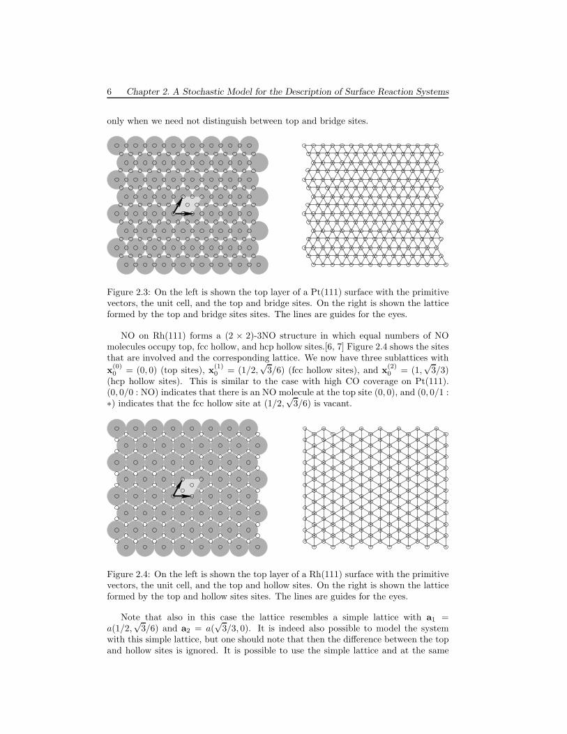
At high coverages the repulsion between the CO molecules forces some of themto bridge sites.[5] Figure 2.3 shows the new lattice. We have now for sublattices with
x(0)0 = (0, 0), x
(1)0 = (1/2, 0), x
(2)0 = (1/4,
√3/4), x
(3)0 = (3/4,
√3/4). The first one is
for the top sites. The others are for the three sublattices of bridge sites. The figureshows that the lattice looks like a simple lattice. Indeed we can regard as such, but
6 Chapter 2. A Stochastic Model for the Description of Surface Reaction Systems
only when we need not distinguish between top and bridge sites.
Figure 2.3: On the left is shown the top layer of a Pt(111) surface with the primitivevectors, the unit cell, and the top and bridge sites. On the right is shown the latticeformed by the top and bridge sites sites. The lines are guides for the eyes.
NO on Rh(111) forms a (2 × 2)-3NO structure in which equal numbers of NOmolecules occupy top, fcc hollow, and hcp hollow sites.[6, 7] Figure 2.4 shows the sitesthat are involved and the corresponding lattice. We now have three sublattices with
x(0)0 = (0, 0) (top sites), x
(1)0 = (1/2,
√3/6) (fcc hollow sites), and x
(2)0 = (1,
√3/3)
(hcp hollow sites). This is similar to the case with high CO coverage on Pt(111).(0, 0/0 : NO) indicates that there is an NO molecule at the top site (0, 0), and (0, 0/1 :∗) indicates that the fcc hollow site at (1/2,
√3/6) is vacant.
Figure 2.4: On the left is shown the top layer of a Rh(111) surface with the primitivevectors, the unit cell, and the top and hollow sites. On the right is shown the latticeformed by the top and hollow sites sites. The lines are guides for the eyes.
Note that also in this case the lattice resembles a simple lattice with a1 =a(1/2,
√3/6) and a2 = a(
√3/3, 0). It is indeed also possible to model the system
with this simple lattice, but one should note that then the difference between the topand hollow sites is ignored. It is possible to use the simple lattice and at the same
2.1 The lattice gas 7
time retaining the difference between the sites. The trick is to use the labels not justfor the occupancy, but also for indicating the type of site. So instead of labels NO and∗ indicating the occupancy, we use NOt, NOf, NOh, ∗t, ∗f, and ∗h. The last letterindicates the type of site (t stands for top, f for fcc hollow, and h for hcp hollow)and the rest for the occupancy. Instead of (0, 0/0 : NO) and (0, 0/1 : ∗) we have(0, 0 : NOt) and (1, 0 : ∗f), respectively. It depends very much on the reaction whichway of describing the system is more convenient and computationally more efficient.
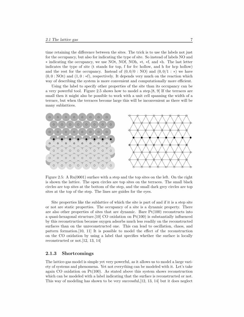
Using the label to specify other properties of the site than its occupancy can bea very powerful tool. Figure 2.5 shows how to model a step.[8, 9] If the terraces aresmall then it might also be possible to work with a unit cell spanning the width of aterrace, but when the terraces become large this will be inconvenient as there will bemany sublattices.
Figure 2.5: A Ru(0001) surface with a step and the top sites on the left. On the rightis shown the lattice. The open circles are top sites on the terraces. The small blackcircles are top sites at the bottom of the step, and the small dark grey circles are topsites at the top of the step. The lines are guides for the eyes.
Site properties like the sublattice of which the site is part of and if it is a step siteor not are static properties. The occupancy of a site is a dynamic property. Thereare also other properties of sites that are dynamic. Bare Pt(100) reconstructs intoa quasi-hexagonal structure.[10] CO oxidation on Pt(100) is substantially influencedby this reconstruction because oxygen adsorbs much less readily on the reconstructedsurfaces than on the unreconstructed one. This can lead to oscillation, chaos, andpattern formation.[10, 11] It is possible to model the effect of the reconstructionon the CO oxidation by using a label that specifies whether the surface is locallyreconstructed or not.[12, 13, 14]
2.1.3 Shortcomings
The lattice-gas model is simple yet very powerful, as it allows us to model a large vari-ety of systems and phenomena. Yet not everything can be modeled with it. Let’s takeagain CO oxidation on Pt(100). As stated above this system shows reconstructionwhich can be modeled with a label indicating that the surface is reconstructed or not.This way of modeling has shown to be very successful,[12, 13, 14] but it does neglect
8 Chapter 2. A Stochastic Model for the Description of Surface Reaction Systems
some aspects of the reconstruction. The reconstructed and the unreconstructed sur-face have very different unit cells, and the adsorption sites are also different.[15, 16]In fact, the unit cell of the reconstructed surface is very large, and there are a largenumber of adsorption sites with slightly different properties. These aspects have beenneglected in the kinetic simulations so far. As these simulations have been quite suc-cessful, it seems that these aspects are not very relevant in this case, but that neednot be always be the case. Catalytic partial oxidation (CPO) takes place at hightemperature at which the surface is so dynamic that all translational symmetry islost. In this case using a lattice to model the kinetics seems inappropriate.
The example of CO on Pt(111) has shown that at high coverage the position atwhich the molecules adsorb change. The reason for this is that these positions are notonly determined by the interactions between the adsorbates and the substrate, but alsoby the interactions between the adsorbates themselves. At low coverages the formerdominate, but at high coverages the latter may be more important. This may leadto adlayer structures that are incommensurate with the substrate.[2] Examples areformed by the nobles gases. These are weakly physisorbed, whereas at high coveragesthe packing onto the substrate is determined by the steric repulsion between them.At low and high coverages different lattices are needed to describe the positions of theadsorbates, but a single lattice describing both the low and the high coverage sites isnot possible. Simulations in which the coverages change from low to high coverageand/or vice versa then cannot be based on a lattice-gas model.
2.2 The Master Equation
2.2.1 Definition
Our treatment of Monte Carlo simulations of surface reactions differs in one veryfundamental aspect from that of other authors; the derivation of the algorithms anda large part of the interpretation of the results of the simulations are based on aMaster Equation
dPα
dt=∑
β
[WαβPβ − WβαPα] . (2.4)
In this equation t is time, α and β are configurations of the adlayer, Pα and Pβ aretheir probabilities, and Wαβ and Wβα are so-called transition probabilities per unittime that specify the rate with which the adlayer changes due to reactions. The MasterEquation is a loss-gain equation. The first term on the right stands for increases inPα because of reactions that change other configurations into α. The second termstands for decreases because of reactions in α. From
d
dt
∑
α
Pα =∑
α
dPα
dt=∑
αβ
[WαβPβ − WβαPα] = 0 (2.5)
we see that the total probability is conserved. (The last equality can be seen byswapping the summation indices in one of the terms.)
The Master Equation can be derived from first principles as will be shown below,and hence forms a solid basis for all subsequent work. There are other advantages aswell. First, the derivation of the Master Equation yields expressions for the transitionprobabilities that can be computed with quantum chemical methods.[17] This makes
2.2 The Master Equation 9
ab-initio kinetics for catalytic processes possible. Second, there are many differentalgorithms for Monte Carlo simulations. Those that are derived from the MasterEquation all give necessarily results that are statistically identical. Those that cannotbe derived from the Master Equation conflict with first principles and should bediscarded. Third, Monte Carlo is a way to solve the Master Equation, but it is notthe only one. The Master Equation can, for example, be used to derive the normalmacroscopic rate equation (see below). In general, it forms a good basis to comparedifferent theories of kinetic quantitatively, and also to compare these theories withsimulations.
2.2.2 Derivation
The Master Equation can be derived by looking at the surface and its adsorbates inphase space. This is, of course, a classical mechanics concept, and one might wonderif it is correct to look at the reactions on an atomic scale and use classical mechanics.The situation here is the same as for the derivation of the rate equations for gasphase reactions. The usual derivations there also use classical mechanics.[18, 19, 20,21, 22] Although it is possible to give a completely quantum mechanical derivationformalism,[23, 24, 25, 26] the mathematical complexity hides much of the importantparts of the chemistry. Besides, it is possible to replace the classical expressions thatwe will get by semi-quantum mechanical ones, in exactly the same way as for gasphase reactions.
A point in phase space completely specifies the positions and momenta of allatoms in the system. In Molecular Dynamics simulations one uses these positions andmomenta at some starting point to compute them at later times. One thus obtainsa trajectory of the system in phase space. We are not interested in that amount ofdetail, however. In fact as was stated before too much detail is detrimental if one isinterested in simulating many reactions. The time interval that one can simulate asystem using Molecular Dynamics is typically of the order of nanoseconds. Reactionsin catalysis have a characteristic time that is many orders of magnitude longer. Toovercome this large difference we need a method that removes the fast processes(vibrations) that determine the time scale of Molecular Dynamics, and leaves us withthe slow processes (reactions). This method looks as follows.
Instead of the precise position of each atom, we only want to know how thedifferent adsorbates are distributed over the sites of a surface. So our physical modelis a lattice. Each lattice point corresponds to one site, and has a label that specifieswhich adsorbate is adsorbed. (A vacant site is simply a special label.) A particulardistribution of the adsorbates over the sites, or, what is the same, a particular labelingof the grid points, we call a configuration. As each point in phase space is a precisespecification of the position of each atom, we also know which adsorbates are atwhich sites; i.e., we know the corresponding configuration. Different points in phasespace may, however, correspond to the same configuration, which differ only in slightvariations of the positions of the atoms. This means that we can partition phase spacein many region, each of which corresponds to one configuration. Reactions are thennothing but motion of the system in phase space from one region to another.
Because it is not possible to reproduce an experiment with exactly the same con-figuration, we are not only not interested in the precise position of the atoms, weare not even interested in specific configurations, but only in characteristic ones. Al-
10 Chapter 2. A Stochastic Model for the Description of Surface Reaction Systems
though there may be differences on a microscopic scale, the behavior of a system ona macroscopic, and often also on a mesoscopic, scale will be the same. So we donot look at individual trajectories in phase space, but we average over all possibletrajectories. This means that we work with a phase space density ρ and a probabilityPα of finding the system in configuration α. These are related via
Pα(t) =
∫
Rα
dq dp
hDρ(q,p, t), (2.6)
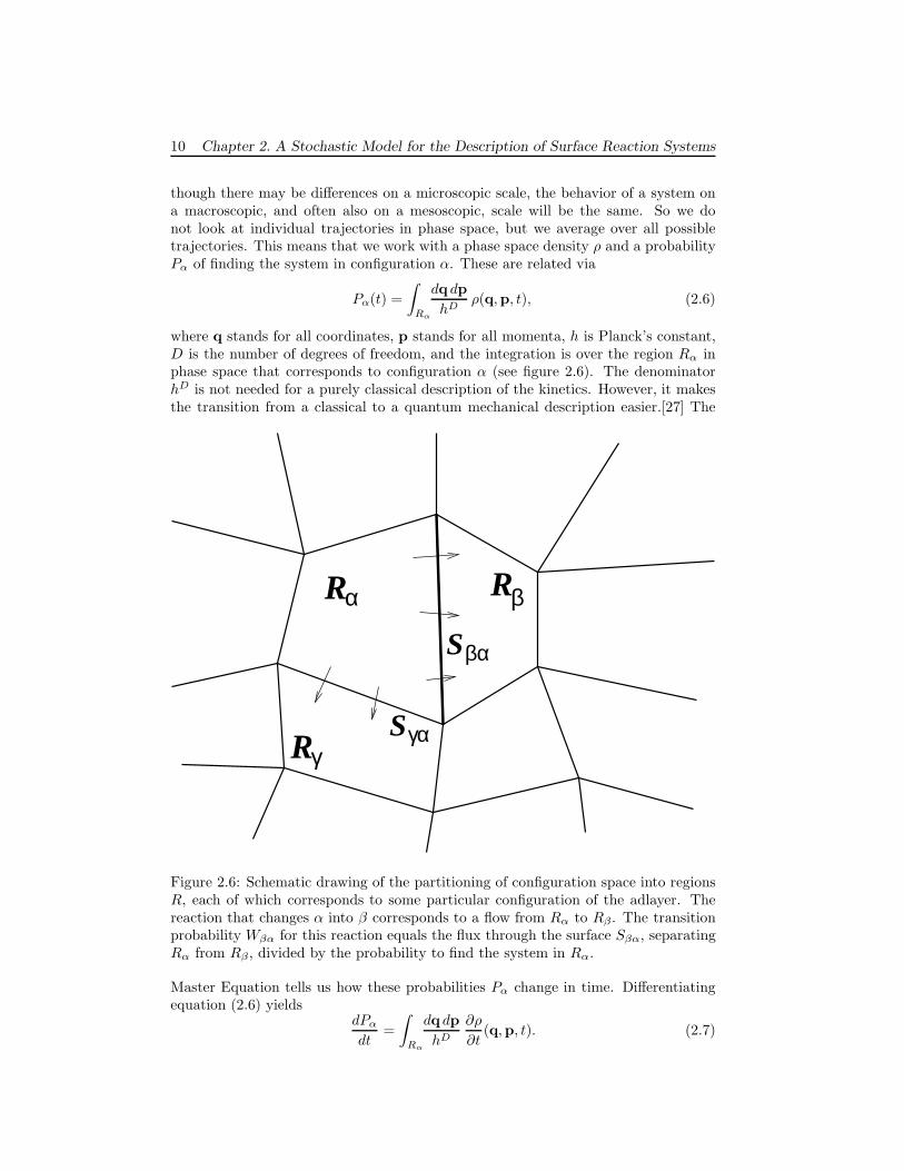
where q stands for all coordinates, p stands for all momenta, h is Planck’s constant,D is the number of degrees of freedom, and the integration is over the region Rα inphase space that corresponds to configuration α (see figure 2.6). The denominatorhD is not needed for a purely classical description of the kinetics. However, it makesthe transition from a classical to a quantum mechanical description easier.[27] The
Rα
Sγα
βαS
Rβ
Rγ
Figure 2.6: Schematic drawing of the partitioning of configuration space into regionsR, each of which corresponds to some particular configuration of the adlayer. Thereaction that changes α into β corresponds to a flow from Rα to Rβ . The transitionprobability Wβα for this reaction equals the flux through the surface Sβα, separatingRα from Rβ , divided by the probability to find the system in Rα.
Master Equation tells us how these probabilities Pα change in time. Differentiatingequation (2.6) yields
dPα
dt=
∫
Rα
dq dp
hD
∂ρ
∂t(q,p, t). (2.7)
2.2 The Master Equation 11
This can be transformed using the Liouville-equation[28]
∂ρ
∂t= −
D∑
i=1
[
∂ρ
∂qi
∂H
∂pi− ∂ρ
∂pi
∂H
∂qi
]
(2.8)
into
dPα
dt=
∫
Rα
dq dp
hD
D∑
i=1
[
∂ρ
∂pi
∂H
∂qi− ∂ρ
∂qi
∂H
∂pi
]
, (2.9)
where H is the system’s classical Hamiltonian. To simplify the mathematics, we willassume that the coordinates are Cartesian and the Hamiltonian has the usual form
H =
D∑
i=1
p2i
2mi+ V (q), (2.10)
where mi is the mass corresponding to coordinate i. We also assume that the areaRα is defined by coordinates only, and that the limits of integration for the momentaare ±∞. Although these assumptions are hardly restrictive, we would like to mentionreference[29] for a more general derivation. The assumptions allow us to go fromphase space to configuration space. (Not to be confused with the configurations ofthe Master Equation.) The first term of equation (2.9) now becomes
∫
Rα
dq dp
hD
D∑
i=1
∂ρ
∂pi
∂H
∂qi=
D∑
i=1
∫
Rα
dq∂V
∂qi
∫ ∞
−∞
dp
hD
∂ρ
∂pi(2.11)
=
D∑
i=1
∫
Rα
dq∂V
∂qi
∫ ∞
−∞
dp1 . . . dpi−1dpi+1 . . . dpD
hD
×[
ρ(pi = ∞) − ρ(pi = −∞)]
= 0,
because ρ has to go to zero for any of its variables going to ±∞ to be integrable. Thesecond term becomes
−∫
Rα
dq dp
hD
D∑
i=1
∂ρ
∂qi
∂H
∂pi= −
∫
Rα
dq dp
hD
D∑
i=1
∂
∂qi
(
pi
miρ
)
. (2.12)
This particular form suggest using the divergence theorem for the integration overthe coordinates.[30] The final result is then
dPα
dt= −
∫
Sα
dS
∫ ∞
−∞
dp
hD
D∑
i=1
nipi
miρ, (2.13)
where the first integration is a surface integral over the surface of Rα, and ni are thecomponents of the outward pointing normal of that surface. Both the area Rα andthe surface Sα are now regarded as parts of the configuration space of the system. Aspi/mi = qi, we see that the summation in the last expression is the flux through Sα
in the direction of the outward pointing normal (see figure 2.6).The final step is now to decompose this flux in two ways. First, we split the
surface Sα into sections Sα = ∪βSβα, where Sβα is the surface separating Rα from
12 Chapter 2. A Stochastic Model for the Description of Surface Reaction Systems
Rβ . Second, we distinguish between an outward flux,∑
i nipi/mi > 0, and an inwardflux,
∑
i nipi/mi < 0. Equation (2.13) can then be rewritten as
dPα
dt=
∑
β
∫
Sαβ
dS
∫ ∞
−∞
dp
hD
(
D∑
i=1
nipi
mi
)
Θ
(
D∑
i=1
nipi
mi
)
ρ (2.14)
−∑
β
∫
Sβα
dS
∫ ∞
−∞
dp
hD
(
D∑
i=1
nipi
mi
)
Θ
(
D∑
i=1
nipi
mi
)
ρ,
where in the first term Sαβ (= Sβα) is regarded as part of the surface of Rβ , andthe ni are components of the outward pointing normal of Rβ . The function Θ is theHeaviside step function.[31] Equation (2.14) can be cast in the form of the MasterEquation
dPα
dt=∑
β
[WαβPβ − WβαPα] , (2.15)
if we define the transition probabilities as
Wαβ =
[
∫
Sαβ
dS
∫ ∞
−∞
dp
hD
(
D∑
i=1
nipi
mi
)
Θ
(
D∑
i=1
nipi
mi
)
ρ
]
/
[∫
Rα
dq
∫ ∞
−∞
dp
hDρ
]
.
(2.16)
The expression for the transition probabilities can be cast in a more familiar formby using a few additional assumptions. We assume that ρ can locally be approximatedby a Boltzmann-distribution
ρ = N exp
[
− H
kBT
]
, (2.17)
where T is the temperature, kB is the Boltzmann-constant, and N is a normalizingconstant. We also assume that we can define Sαβ and the coordinates in such a waythat ni = 0, except for one coordinate i, called the reaction coordinate, for whichni = 1. The integral of the momentum corresponding to the reaction coordinate canthen be done and the result is
Wαβ =kBT
h
Q‡
Q, (2.18)
with
Q‡ ≡∫
Sαβ
dS
∫ ∞
−∞
dp1 . . . dpi−1dpi+1 . . . dpD
hD−1exp
[
− H
kBT
]
, (2.19)
Q ≡∫
Rα
dq
∫ ∞
−∞
dp
hDexp
[
− H
kBT
]
. (2.20)
We see that this is an expression that is formally identical to the Transition-StateTheory (TST) expression for rate constants.[32] There are differences in the definitionof the partition functions Q and Q‡, but even these can be neglected as will be shownin chapter 3.
2.3 Working without a lattice 13
2.3 Working without a lattice
Although the use of a lattice is very important in the theory above, one should realizethat it is really not needed from a theoretical point of view. No reference was made toa lattice in the derivation of the Master Equation, and indeed one can use the MasterEquation also for reactive systems that do no have translational or any other kind ofsymmetry.
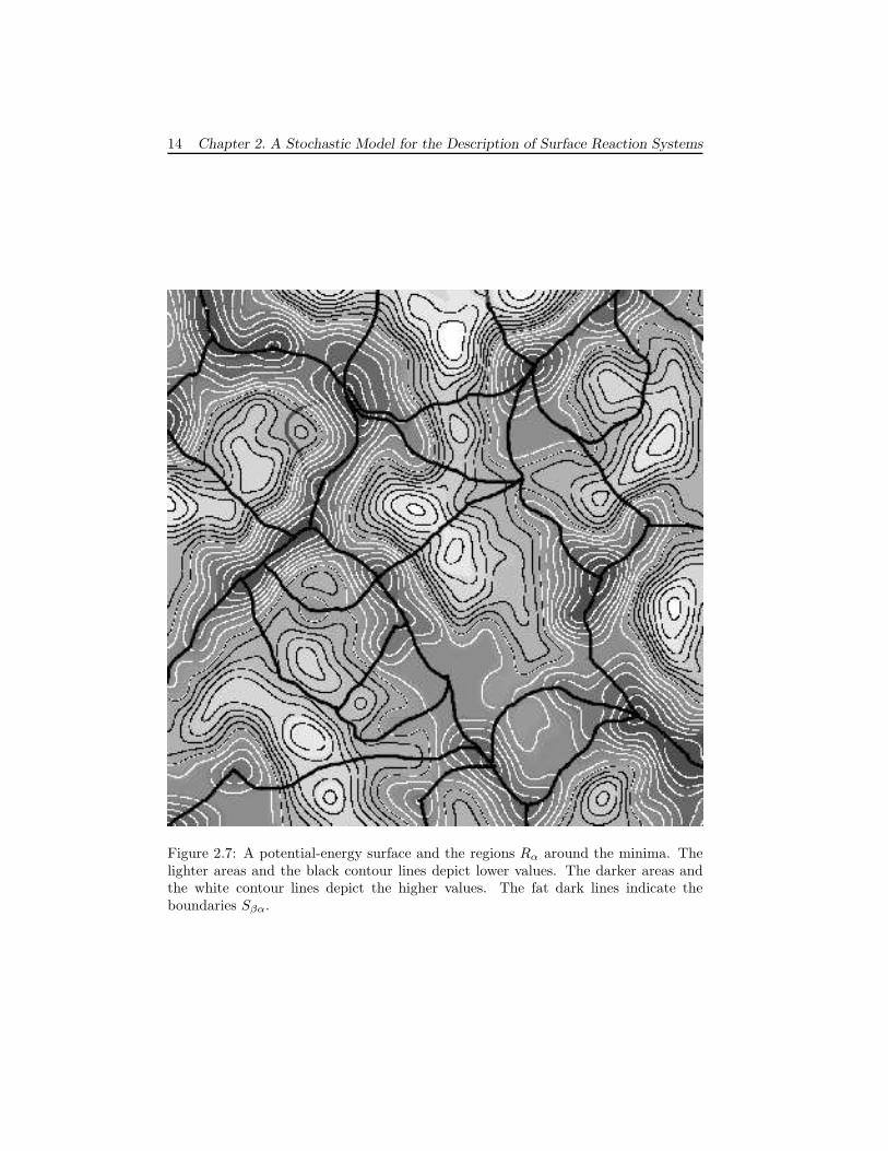
The idea is to look at the potential-energy surface (PES) of a system,[33] andassociate each “configuration” α with a minimum of the PES. The region Rα consistsof the points in phase space around the minimum (see figure 2.7). (As before themomenta can have any value.) The precise position of the surfaces Sβα are hardto determine. In Variational Transition-State Theory (VTST) they are chosen tominimize the flux,[18, 19, 20, 21, 22] but a more pragmatic approach would be toput Sβα at the saddle point of the PES that separates minimum α from β. Thederivation in section 2.2.2 does not change, and we get a Master Equation describingprocesses/reactions corresponding to transitions between the minima of the PES.Again the fast motions in the system have been removed.
The advantage of a system with translation symmetry has to do with the numberof different transition probabilities W . For the general case based on minima of thePES there is a different transition probability for each transition. For reactions on asurface the situation is simpler, because the same reaction occurring at different sitescorresponds to different configuration changes but has the same transition probability.
14 Chapter 2. A Stochastic Model for the Description of Surface Reaction Systems
Figure 2.7: A potential-energy surface and the regions Rα around the minima. Thelighter areas and the black contour lines depict lower values. The darker areas andthe white contour lines depict the higher values. The fat dark lines indicate theboundaries Sβα.
Chapter 3
How to Get the TransitionProbabilities?
The Master Equation is only useful if one knows the transition probabilities. Thereare basically two ways to get them. One way is to calculation them. The other is toderive them from experimental data.
3.1 Quantum chemical calculations of transition prob-
abilities
There are three difference between expressions (2.19) and (2.20) for the partitionfunction and those of TST.[32] The first is the absence of an exponential factor of theform exp(−Ebar/kBT ), the second is the boundaries of the integrations, and the thirdis the absence of a reference to a transition state. We deal with the boundaries first.Very often these can simply be removed. Define q(min) as the point in Rα at whichV is minimal, and approximate V in Rα by
Vharm(q) = V (q(min)) +1
2
∑
i,j
(qi − q(min)i )
∂2V
∂qi∂qj(q(min))(qj − q
(min)j ). (3.1)
This is the harmonic approximation. A very common situation is the following. Vharm
differs from V only appreciably where V − V (q(min)) is large with respect to thethermal energy kBT . Because of the Boltzmann-factor in the integrals we can replaceV by Vharm in the integrals. The integration over Rα can then also be extended toinfinity. The reason for this is that, in the region that has been added to the integral,the Boltzmann-factor with Vharm is so small that the added part is negligible. Q thusbecomes the normal expression for the classical partition function.
Note that we do not really need to make the harmonic approximation. Anhar-monicities can be included. Instead of Vharm we can use any approximation to Vthat is accurate at q unless V (q − V (q(min)) ≫ kBT , and the approximation shouldgive negligible new contributions to the integrals when the boundaries are extendedbeyond Rα.
For Q‡ we can draw the same conclusion. We restrict ourselves to Sαβ and itsextension defined by the coordinates used, and q(min) is the point on Sαβ where V is
15
16 Chapter 3. How to Get the Transition Probabilities?
minimal. The rest of the reasoning is then the same as for Q. This also explains an-other difference with TST. The exponential factor is obtained by taking the V (q(min))out off the integrals for Q and Q‡. This immediately gives the exponential factor withEbar equal to the difference between the minima of V on Sαβ and in Rα.
There are two corrections to equation (2.16) that one might want to make. Thefirst has to do with dynamical factors;[34, 35] i.e., trajectories leave Rα, cross thesurface Sβα, but then immediately return to Rα. Such a trajectory contributes tothe transition probability Wβα, but is not really a reaction. We can correct for thisas in Variational Transition-State Theory (VTST) by shifting Sβα along the surfacenormals.[21, 22] This is related to the absence of any reference to any transition stateso far. Indeed, if the Sβα can be chosen more or less arbitrarily provided the expressionfor Q‡ is corrected for the dynamical factors. Using the VTST approach Sβα will bewell-defined. It turns out that with VTST the transition state (i.e., the saddle pointbetween the minima in Rα and Rβ) is generally very close to Sβα, and taking Sβα sothat it contains the transition state is often a very good approximation.[21, 22]
The second correction is for some quantum effects. Equation (2.18) indicates oneway to include them. We can simply replace the classical partition functions by theirquantum mechanical counterparts. (It is possible, of course, to do the integrals overthe momenta in equations (2.19) and (2.20). The reason why we did not do thatwas to retain the correspondence between classical and quantum partition functions.)This does not correct for tunneling and interference effects, however. Inaccuraciesdue to tunneling, interference, and dynamic effects are not specific for the transitionprobabilities of the Master Equation. TST expressions have them too. As theseeffects are often small, this means that in practice one can use TST expressionsto calculate the the transition probabilities of the Master Equation using quantumchemical methods in the same way as one calculates rate constants provided that thepartition functions get the dominant contribution from a region in the integrationrange surrounding a minimum.
In the harmonic approximation we can write Q as
Q = e−Vmin/kBT∏
i
qv(ωi) (3.2)
with Vmin the minimum of the potential energy in Rα. The vibrational partitionfunction qv is given by
qv(ω) =kBT
hω(3.3)
classically, or
qv(ω) =e
12hω/kBT
1 − ehω/kBT(3.4)
quantum mechanically.[27, 28] The frequencies ωi are the normal mode frequencies.[36,37] Similarly we find for Q‡
Q‡ = e−V ′
min/kBT∏
j
qv(ω′j) (3.5)
with V ′min the minimum of the potential energy on Sβα and ω′
j the non-imaginarynormal mode frequencies at the transition state. Combining these results yields
Wβα =kBT
h
∏
j qv(ω′j)
∏
i qv(ωi)e−Ebar/kBT (3.6)
3.1 Quantum chemical calculations of transition probabilities 17
with Ebar = V ′min − Vmin.
It is very interesting to look in more detail at the case when it is not correctto extend the boundaries of the integrals. When the substrate has a closed-packedstructure the potential-energy surface may be quite flat parallel to the surface. If thatis the case there may be substantial contributions to the partition function up to theboundaries of the integrals. It is then not possible to apply the reasoning above. Wewill look at two examples; both dealing with simple desorption of an atom. In thefirst example the potential is completely flat parallel to the surface for all distancesof the atom to the surface. In the second example the potential only becomes flat atthe transition state.
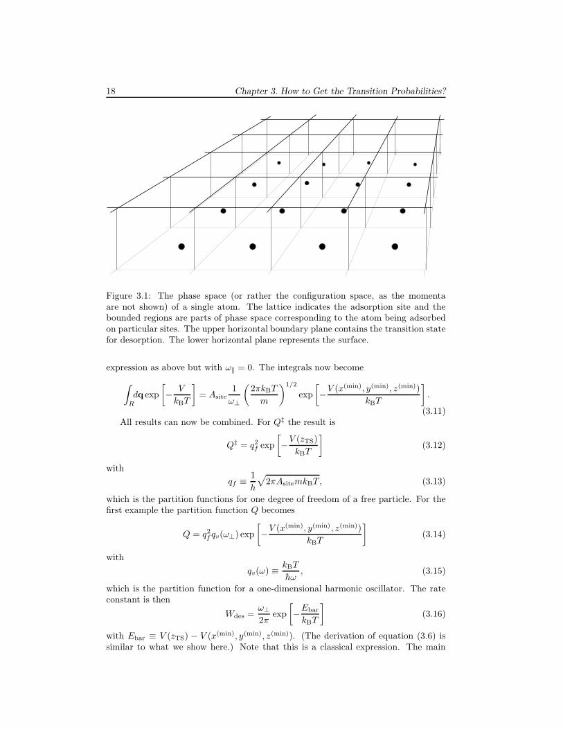
Because dealing with a phase space of many atoms is inconvenient, we restrictourselves to just one atom on the surface and calculate the transition state for des-orption for that single atom. This is the usual approach; try to minimize the numberof particles. The step to many atoms on the surface is made by assuming that thetransition probability is independent on the number of atoms. This is correct if thereare no lateral interactions, as we are assuming here. The case with lateral interactionswill be discussed later.
Figure 3.1 show regions in phase space corresponding to an atom adsorbed ondifferent sites. Crossing the upper horizontal plane bounding a region constitutesa desorption. Crossing one of the vertical planes bounding a region constitutes adiffusion to another site. The integrals of each momentum in the expression for thepartition functions Q and Q‡ become
∫ ∞
−∞
dp
hexp
[
− p2
2mkBT
]
=1
h
√
2πmkBT . (3.7)
The integrals of the coordinates for Q‡ become
∫
Sαβ
dS exp
[
− V
kBT
]
= Asite exp
[
−V (zTS)
kBT
]
, (3.8)
where zTS is the value of the coordinate perpendicular to the surface at the transitionstate for desorption, and Asite is the area of the horizontal boundary plane of a regionor the area of a single site.
The integrals of the coordinates for Q differ between our two examples. If thepotential has a well-defined minimum near the adsorption site, then we can use theharmonic approximation (this is our second example).
Vharm = V (x(min), y(min), z(min)) (3.9)
+1
2mω2
‖(x − x(min))2 +1
2mω2
‖(y − y(min))2 +1
2mω2
⊥(z − z(min))2.
The integrals become
∫
R
dq exp
[
− V
kBT
]
=1
ω2‖ω⊥
(
2πkBT
m
)3/2
exp
[
−V (x(min), y(min), z(min))
kBT
]
. (3.10)
If the potential is flat parallel to the surface (this is our first example), then we canuse the harmonic approximation only perpendicular to the surface. We get the same
18 Chapter 3. How to Get the Transition Probabilities?
Figure 3.1: The phase space (or rather the configuration space, as the momentaare not shown) of a single atom. The lattice indicates the adsorption site and thebounded regions are parts of phase space corresponding to the atom being adsorbedon particular sites. The upper horizontal boundary plane contains the transition statefor desorption. The lower horizontal plane represents the surface.
expression as above but with ω‖ = 0. The integrals now become
∫
R
dq exp
[
− V
kBT
]
= Asite1
ω⊥
(
2πkBT
m
)1/2
exp
[
−V (x(min), y(min), z(min))
kBT
]
.
(3.11)All results can now be combined. For Q‡ the result is
Q‡ = q2f exp
[
−V (zTS)
kBT
]
(3.12)
with
qf ≡ 1
h
√
2πAsitemkBT , (3.13)
which is the partition functions for one degree of freedom of a free particle. For thefirst example the partition function Q becomes
Q = q2f qv(ω⊥) exp
[
−V (x(min), y(min), z(min))
kBT
]
(3.14)
with
qv(ω) ≡ kBT
hω, (3.15)
which is the partition function for a one-dimensional harmonic oscillator. The rateconstant is then
Wdes =ω⊥
2πexp
[
−Ebar
kBT
]
(3.16)
with Ebar ≡ V (zTS) − V (x(min), y(min), z(min)). (The derivation of equation (3.6) issimilar to what we show here.) Note that this is a classical expression. The main
3.1 Quantum chemical calculations of transition probabilities 19
quantum effect is included by replacing the partition function qv by its quantummechanical counterpart.[27, 28]
qv(ω) =e
12hω/kBT
1 − ehω/kBT(3.17)
If kBT ≪ hω⊥ then qv = exp[− 12 hω⊥/kBT ] is a good approximation so that
Wdes =kBT
hexp
[
−Ebar
kBT
]
(3.18)
with Ebar = V (zTS)−[V (x(min), y(min), z(min))+ 12 hω⊥]. The last term is the zero-point
energy of the adsorbed atom.[38]For the second example we have
Q = qv(ω⊥)q2v(ω‖) exp
[
−V (x(min), y(min), z(min))
kBT
]
(3.19)
so that
Wdes =2πAsiteω⊥ω2
‖
kBTexp
[
−Ebar
kBT
]
(3.20)
classically, and
Wdes =2πAsitem(kBT )2
h3exp
[
−Ebar
kBT
]
(3.21)
quantum mechanically if ω⊥, ω‖ ≫ kBT/h and with Ebar = V (zTS)−[V (x(min), y(min), z(min))+
hω‖ + 12 hω⊥].
The expressions above show that the main properties that should be determinedin a quantum chemical calculation is the barrier Ebar, and the vibrational frequen-cies ω⊥ and possible ω‖. It is interesting to calculate the preexponential factorsin equations (3.18) and (3.21), assuming that the vibrational excitation energiesare large compared to the thermal energies. This is probably correct for Xe des-orption from Pt(111). If there is little corrugation (ω‖ ≈ 0) then we have to useequation (3.18). The preexponential factor in that expression at T = 100 K equalskBT/h = 2.1 · 1012 s−1. If we assume that Xe adsorbs strongly to a particular sitethen we are dealing with equation (3.21). With m = 2.2 ·10−25 kg, A = 6.4 ·10−20 m2
we get 2πAm(kBT )2/h3 = 5.8 · 1014 s−1.The usual way to write a rate constant is ν exp[−Eact/kBT ]. (We will see that rate
constants and transition probabilities are very similar. We will from now on often usethe term rate constant instead of transition probabilities.) The preexponential factorν and the activation energy Eact is usually assumed to be independent of temperature.This is done certainly in the experimental literature when one determines these kineticparameters from measurements of rate constants as a function of temperature. Usingthis form for the rate constant one may define the activation energy as
Eact ≡ − d lnW
d(1/kBT )= kBT 2 d lnW
dT, (3.22)
where W is a transition probability, and the preexponential factor as
ν ≡ W exp
[
Eact
kBT
]
. (3.23)
20 Chapter 3. How to Get the Transition Probabilities?
With these definitions the kinetic parameters are often found not to be temperatureindependent. Getting back to desorption from a surface in which the corrugation ofthe potential is negligible we find from equation (3.18) that Eact = Ebar+kBT and ν =ekBT/h. For desorption from a surface with corrugation we find from equation (3.21)that Eact = Ebar + 2kBT and ν = 2πAsite(ekBT )2/h3. We see that indeed theactivation energy and the preexponential factor are temperature dependent. Thedependence for the activation energy is small, because the thermal energy kBT isgeneral small compared to the barrier height Ebar. The effect on the preexponentialfactor seems larger, but one should remember that rate constants vary over manyorders of magnitude, and the effect of temperature on the preexponential factor affectsthe order of magnitude of the preexponential factor only a little. Moreover, there is acompensation effect . Increasing the temperature increases the preexponential factor,but also the activation energy, so the effect on the rate constant is reduced.
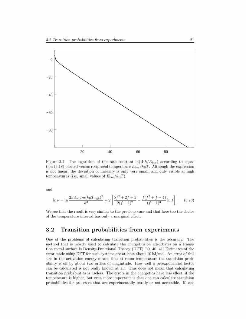
The experimental determination of the activation energy and preexponential factordoes not use the expression above of course. Experimentalists plot the logarithm ofa rate constant versus the reciprocal temperature and then fit a linear curve to it.This is something we can do as well with equations (3.18) and 3.21. The result willdepend on the temperature interval on which we do the fit, but we will see thatthe dependence is generally small. If we take, for example, equation (3.18) and plotln(hWdes/Ebar) versus β ≡ Ebar/kBT we get figure 3.2. The function that is plottedin this figure is −β − ln(β). Although this function is not linear, we see that only ifβ is small ln(β) is of similar size as β and deviations of non-linearity are noticeable.This only occurs at such high temperature that β < 1, whereas experimentally oneusually works at temperatures with β ≫ 1.
If we fit ν exp[−Eact/kBT ] to equation (3.18) on the interval [Tlow, Thigh] in theexperimental way, we have to minimize
∫ 1/Tlow
1/Thigh
d
(
1
T
)[
lnWdes − ln ν +Eact
kBT
]2
(3.24)
as a function of ln ν and Eact. The mathematics is straightforward, and the result is
Eact = Ebar
[
1 +3kBThigh
Ebar
f2 − 1 − 2f ln f
(f − 1)3
]
, (3.25)
with f = Thigh/Tlow. The second term in square brackets is small because the barrierheight is generally much larger than the thermal energy. The factor with the f ’sdecreases monotonically from 1 for f = 1 to 0 for f → ∞. For the preexponentialfactor we find
ln ν = lnkBThigh
h+
[
5f2 + 2f + 5
2(f − 1)2− f(f2 + f + 4)
(f − 1)3ln f
]
. (3.26)
The expression in square brackets with the f ’s varies from 1 for f = 1 to −∞ forf → ∞ and becomes 0 at f ≈ 5.85. This means that it is generally small comparedto the first term in the expression for ln ν.
If we fit ν exp[−Eact/kBT ] to equation (3.21) on the interval [Tlow, Thigh] in theexperimental way, we get
Eact = Ebar
[
1 +6kBThigh
Ebar
f2 − 1 − 2f ln f
(f − 1)3
]
, (3.27)
3.2 Transition probabilities from experiments 21
−80
−60
−40
−20
0
20 40 60 80
Figure 3.2: The logarithm of the rate constant ln(Wh/Ebar) according to equa-tion (3.18) plotted versus reciprocal temperature Ebar/kBT . Although the expressionis not linear, the deviation of linearity is only very small, and only visible at hightemperatures (i.e., small values of Ebar/kBT ).
and
ln ν = ln2πAsitem(kBThigh)
2
h3+ 2
[
5f2 + 2f + 5
2(f − 1)2− f(f2 + f + 4)
(f − 1)3ln f
]
. (3.28)
We see that the result is very similar to the previous case and that here too the choiceof the temperature interval has only a marginal effect.
3.2 Transition probabilities from experiments
One of the problems of calculating transition probabilities is the accuracy. Themethod that is mostly used to calculate the energetics on adsorbates on a transi-tion metal surface is Density-Functional Theory (DFT).[39, 40, 41] Estimates of theerror made using DFT for such systems are at least about 10 kJ/mol. An error of thissize in the activation energy means that at room temperature the transition prob-ability is off by about two orders of magnitude. How well a preexponential factorcan be calculated is not really known at all. This does not mean that calculatingtransition probabilities is useless. The errors in the energetics have less effect, if thetemperature is higher, but even more important is that one can calculate transitionprobabilities for processes that are experimentally hardly or not accessible. If, one
22 Chapter 3. How to Get the Transition Probabilities?
the other hand, one can obtain transition probabilities from an experiment, then thevalue that is obtained is generally more reliable than one calculated.
In general, one has to deal with a system in which several reactions can takeplace at the same time. The crude approach to obtain transition probabilities fromexperiments is then to try to fit all transition probabilities to the experiments atthe same time. This is often not a good idea. First of all such a procedure can bequite complicated. The data that one gets from an experiment are seldom a linearfunction of the transition probabilities. Consequently the fitting procedure consists ofminimizing a nonlinear function that stands for the difference between experimentaland the calculated or simulated data. Such a function normally has many localminima, and it is very hard to find the best set of transition probabilities. But thisisn’t even the most important drawback. Although one may be able to do a very goodfit of the experimental data, this need not mean that the transition probabilities aregood; given enough fit parameters, one can fit anything.
Deriving kinetic parameters from experiments does work well, when one has anexperiment of a single simple process that can be described by just one or two param-eters. The process should be simple in the sense that one has an analytical expressionwith which one can derive relatively easily the kinetic parameters given experimentaldata. The analytical expression should be exact or at least a very good approxi-mation. If one has to deal with a reaction system that is complicated and consistsof many reactions, then one should try to get experiments that measure just oneof the reactions. For example, in CO oxidation one has at least adsorption of CO,dissociative adsorption of oxygen, and the formation of CO2. Instead of trying to fitrate constants of these three reactions simultaneously, one should look at experimentsthat show only one of these reactions. An experiment that only measures stickingcoefficients as a function of CO pressure can be used to get the CO adsorption rateconstant. The following sections show a number of processes which can be used toget kinetic parameters, and we show how to get the parameters.
3.2.1 Relating macroscopic properties to microscopic processes
The analytical expressions mentioned above should relate some property that is mea-sured to the transition probabilities. We will address first the general relation. Thisrelation is exact, but often not very useful. In the next sections we will show situa-tions were the general relation can be simplified either exactly or with the use of someapproximation.
If a system is in a well-defined configuration then a macroscopic property cangenerally be computed easily. For example, the number of molecules of a particulartype in the adlayer can be obtained simply be counting. If the property that we areinterested in is denoted by X , then its value when the system is in configuration α isgiven by Xα. As our description of the system uses probabilities for the configurations,we have to look at the expectation value of X , which is given by
⟨
X⟩
=∑
α
PαXα. (3.29)
Kinetic experiment measure changes, so we have to look at d⟨
X⟩
/dt. This is given
3.2 Transition probabilities from experiments 23
byd⟨
X⟩
dt=∑
α
dPα
dtXα, (3.30)
because Xα is a property of a fixed configuration. We can remove the derivative ofthe probability using the Master Equation. This gives us
d⟨
X⟩
dt=
∑
αβ
[WαβPβ − WβαPα] Xα,
=∑
αβ
WαβPβ [Xα − Xβ] . (3.31)
The second step is obtained by swapping the summation indices. The final result canbe regarded as the expectation value of the change of X in the reaction β → α timesthe rate constant of that reaction. This general equation forms the basis for derivingrelations between macroscopic properties and transition probabilities.
3.2.2 Unimolecular desorption
Suppose we have atoms or molecules that adsorb onto one particular type of site. Weassume that we have of surface of area A with S adsorption sites. If Nα is the numberof atoms/molecules in configuration α then
d⟨
N⟩
dt=∑
αβ
WαβPβ [Nα − Nβ] . (3.32)
Diffusion does not change the number atoms/molecules, and it does not matter inthis case whether we include it or not. The only relevant process that we look at isdesorption. For the summation over α we have to distinguish between two types ofterms; the ones where α can originate from β by a desorption, and the ones whereit cannot. The latter terms have Wαβ = 0 and so they to not contribute to thesum. The former do contribute and we have Wαβ = Wdes, with Wdes the transitionprobability for desorption, and Nα−Nβ = −1. So all these non-zero terms contributeequally to the sum for a given configuration β. Moreover, the number of these termsis equally to the number of atoms/molecules in β that can desorb, because eachdesorbing atom/molecule yields a different α. So
d⟨
N⟩
dt= −Wdes
∑
β
PβNβ = −Wdes
⟨
N⟩
. (3.33)
This is an exact expression. Dividing by the number of sites S gives the rate equationfor the coverage θ =
⟨
N⟩
/S.dθ
dt= −Wdesθ. (3.34)
If we compare this to the macroscopic rate equation dθ/dt = −kdesθ with kdes themacroscopic rate constant, we see that kdes = Wdes.
For isothermal desorption kdes does not depend on time and the solution to therate equation is
θ(t) = θ(0) exp[−kdest], (3.35)
24 Chapter 3. How to Get the Transition Probabilities?
where θ(0) is the coverage at time t = 0. Kinetic experiments often measure rates,and for the desorption rate we have
dθ
dt(t) = −kdesθ(0) exp[−kdest]. (3.36)
We can now obtain the rate constant by measuring, for example, the rate of desorptionas a function of time and plotting minus the logarithm of the rate as a function oftime. Because
ln
[
−dθ
dt(t)
]
= ln[kdesθ(0)] − kdest, (3.37)
we can obtain the rate constant which equals minus the slope of the straight line.The same would hold if we would plot the logarithm of the coverage as a function oftime. Because of the equality this immediately also yields the transition probabilityto be used in a simulation.
If the rate constant depends on time then solving the rate equation is often muchmore difficult. We can always rewrite the rate equation as
1
θ
dθ
dt
d ln θ
dt= −kdes. (3.38)
Integrating this equation yields
ln θ(t) − ln θ(0) = −∫ t
0
dt′kdes(t′), (3.39)
or
θ(t) = θ(0) exp
[
−∫ t
0
dt′kdes(t′)
]
. (3.40)
Whether of not we can get an analytical solution depends on whether we can determinethe integral. In Temperature-Programmed Desorption experiments we have
kdes(t) = ν exp
[
− Eact
kB(T0 + Bt)
]
(3.41)
with Eact an activation energy, ν a preexponential factor, kB the Boltzmann-factor,T0 the temperature at time t = 0, and B the heating rate. The integral can becalculated analytically. The result is
∫ t
0
dt′ ν exp
[
− Eact
kB(T0 + Bt′)
]
= Ω(t) − Ω(0) (3.42)
with
Ω(t) =ν
B(T0 + Bt)E2
[
Eact
kB(T0 + Bt)
]
, (3.43)
where E2 is an exponential integral.[42] Although this solution has been derived sometime ago,[43] it has not yet been used in the analysis of experimental spectra, butthere are several numerical techniques that work well for such simple desorption.[44]Note that we have not made any approximations here and the transition probabilityWdes that we obtain will be exact except for experimental errors.
3.2 Transition probabilities from experiments 25
3.2.3 Unimolecular adsorption
We start with the simplest case in which the adsorption rate is proportional to thenumber of vacant sites, which is called Langmuir adsorption. We will only indicate inthis section in what way in the common situation in which the adsorption is higherthan expected based on the number of vacant sites differs.[3, 32, 45] This so-calledprecursor-mediated adsorption is really a composite process, and has to be treatedwith the knowledge presented in various sections of this chapter.
Again suppose we have atoms or molecules that adsorb onto one particular typeof site. We assume that we have a surface of area A with S adsorption sites. If Nα isthe number of atoms/molecules in configuration α then again
d⟨
N⟩
dt=∑
αβ
WαβPβ [Nα − Nβ] . (3.44)
Diffusion can again be ignored. For the summation over α we have to distinguishbetween two types of terms; the ones in which α can originate from β by a adsorption,and the ones it cannot. The latter terms have Wαβ = 0 and so they to not contributeto the sum. The former do contribute and we have Wαβ = Wads, with Wads thetransition probability for adsorption, and Nα − Nβ = 1. So all these non-zero termscontribute equally to the sum for a given configuration β. Moreover, the number ofthese terms is equally to the number of vacant sites in β onto which the moleculescan adsorb, because each adsorption yields a different α. The number of vacant sitesin configuration β equals S − Nβ , so
d⟨
N⟩
dt= Wads
∑
β
Pβ(S − Nβ) = Wads(S −⟨
N⟩
). (3.45)
Dividing by the number of sites S gives the rate equation for the coverage θ =⟨
N⟩
/S.
dθ
dt= −Wdes(1 − θ). (3.46)
If we compare this to the macroscopic rate equation dθ/dt = kads(1− θ) with kads themacroscopic rate constant, we see that kads = Wads.
So far adsorption is almost the same as desorption. The only difference is wherewe had θ for desorption we have 1−θ for adsorption on the right-hand-side of the rateequation. An importance difference now arises however. Whereas the macroscopicrate constant for desorption kdes is an basic quantity in kinetics of surface reactions,kads is generally related to other properties. This is because the adsorption processconsists of atoms or molecules impinging on the surface, and that is something thatcan be described very well with kinetic gas theory.
Suppose that the pressure of the gas is P and its temperature T , then the numberof molecules F hitting a surface of unit area per unit time is given by[27, 28]
F =P√
2πmkBT(3.47)
with m the mass of the atom or molecule. Not every atom or molecule that hitsa surface will stick to it. The sticking coefficient σ is defined as the ratio of the
26 Chapter 3. How to Get the Transition Probabilities?
number of molecules that stick to the total number hitting the surface. It can also belooked upon as the probability that an atom or molecule hitting the surface sticks.The change in the number of molecules in an area A due to adsorption can then bewritten as the vacant area times the flux F times the sticking coefficient σ. The vacantarea equals to area A times the fraction of sites in that area that is not occupied.This all leads to
d⟨
N⟩
dt= A(1 − θ)Fσ. (3.48)
If we compare this to the equations above we find
Wads =AFσ
S=
PAsiteσ√2πmkBT
, (3.49)
where Asite is the area of a single site.
Adsorption described so far is proportional to the number of vacant sites. Exper-iments measure the rate of adsorption and with the expressions derived above onecan calculate the microscopic rate constant Wads. However, it is often found thatthe rate of adsorption starts at a certain value for a bare surface and then hardlychanges when particles adsorb until the surface is almost completely covered at whichtime it suddenly drops to zero. This behavior is generally explained by describing theadsorption as a composite process.[3, 32, 45] A molecule impinging unto the surfaceadsorbs with the probability σ when the site it hits is vacant just as before. However, amolecule that hits a site that is already occupied need not be scattered. It can adsorbindirectly. It first adsorbs, with a certain probability, in a second adsorption layer.Then it starts to diffuse over the surface in this second layer. It can desorb at a laterstage, or, and that’s the important part, it can encounter a vacant site and adsorbthere permanently. This last part can increase the adsorption rate substantially whenthere are already many sites occupied. The precise dependence of the adsorption rateon the coverage θ is determined by the rate of diffusion, by the rate of adsorptiononto the second layer, and by the rate of desorption from the second layer. If thereare factors that affect the structure of the first adsorption layer, e.g. lateral interac-tion, then these too influence the adsorption rate. If the adsorption is not direct, onetalks about a precursor mechanism. A precursor on top of an adsorbed particle is anextrinsic precursor. An intrinsic precursor can be found on top of a vacant site.[46]The precursor mechanism will not always be operative for a bare surface; i.e., thereis not always an intrinsic precursor. This means that we can use equation (3.49) ifwe take for σ the sticking coefficient for adsorption on a bare surface.
3.2.4 Unimolecular reactions
With the knowledge of simple desorption and adsorption given above it is now easyto derive an expression for the rate constant Wuni for a unimolecular reaction in termof a macroscopic rate constant. In fact the derivation is exactly the same as for thedesorption. Desorption changes a site from A to ∗, whereas a unimolecular reactionchanges it to B. Replace ∗ by B in the expression for the desorption (and Wdes byWuni of course) and you have the correct expression. As the expression for desorptiondo not contain a ∗, the procedure is trivial and we find Wuni = kuni where kuni is therate constant from the macroscopic rate equation.
3.2 Transition probabilities from experiments 27
3.2.5 Diffusion
We treat diffusion as any other reaction, but experimentally one doesn’t look atchanges in coverages but at displacements of atoms and molecules. We will thereforealso look here at how the position of a particle changes.
We assume that we have only one particle on the surface, so that the particle’smovement is not hindered by any other particle. We also assume that we have asquare grid with axis parallel to the x- and the y-axis and that the distance betweengrid points is given by a. We will later look at other grids. If xα is the x-coordinateof the particle in configuration α, then
d⟨
x⟩
dt=∑
αβ
WαβPβ [xα − xβ ]. (3.50)
The x-coordinate change because the particle hops from one to another site. Whenit hops we have xα − xβ = a,−a, and 0 for a hop along the x-axis towards largerx, a hop along the x-axis towards smaller x, or a hop perpendicular to the x-axis,respectively. All these hops have a rate constant Whop and are equally likely. Thismeans d
⟨
x⟩
/dt = 0. The same holds for the y-coordinate.More useful is to look at the square of the coordinates. We then find
d⟨
x2⟩
dt=∑
αβ
WαβPβ [x2α − x2
β ]. (3.51)
Now we have x2α−x2
β = 2axβ +a2,−2axβ +a2, and 0, respectively. Because the hopsare still equally likely, we have
d⟨
x2⟩
dt= 2Whopa2. (3.52)
We find the same for the y-coordinate. The macroscopic equation for diffusion is
d⟨
x2 + y2⟩
dt= 4D, (3.53)
with D the diffusion coefficient. From this we see that we have Whop = D/a2.On a hexagonal grid a particle can hop in six different directions for which xα −
xβ = a, a/2,−a/2,−a,−a/2, and a/2 and yα−yβ = 0, a√
3/2, a√
3/2, 0,−a√
3/2, and −a√
3/2. From this we get again d⟨
x⟩
/dt = 0. For the squared displacement we findx2
α−x2β = 2axβ+a2, axβ+a2/4,−axβ+a2/4,−2axβ+a2,−axβ+a2/4, axβ+a2/4. This
yields again d⟨
x2⟩
/dt = 2Whopa2. We find the same expression for the y-coordinate,
so that also for a hexagonal grid Whop = D/a2. The same expression holds for atrigonal grid. The derivation is identical to the ones for the square and hexagonalgrids.
3.2.6 Bimolecular reactions
For all of the processes we have looked at so far it was possible to derive the macro-scopic equations from the the Master Equation exactly. This is not the case forbimolecular reactions. Bimolecular reactions will give rise to an infinite hierarchy of
28 Chapter 3. How to Get the Transition Probabilities?
macroscopic rate equations. There are two bimolecular reactions we will consider:A + B and A + A. The problem we have mentioned above is the same for both re-actions, but there is a small difference in the derivation of a numerical factor in themacroscopic rate equation. We will start with the A + B reaction.
We look at the number of A’s. The expressions for the number of B’s can beobtained by replacing A’s by B’s and B’s by A’s in the following expressions. Wehave
d⟨
N (A)⟩
dt=∑
αβ
WαβPβ
[
N (A)α − N
(A)β
]
, (3.54)
where N(A)α stands for the number of A’s. If α can originate from β by a A + B
reaction, then Wαβ = Wrx, otherwise Wαβ = 0. If such a reaction is possible, then
N(A)α − N
(A)β = −1. The problem now is with the number of configurations α that
can be obtained from β by a reaction. This number is equal to the number of AB
pairs N(AB)β . This leads then to
d⟨
N (A)⟩
dt= −Wrx
∑
β
PβN(AB)β = −Wrx
⟨
N (AB)⟩
. (3.55)
We get the same right-hand-side for the change in the number of B’s. We see thaton the right-hand-side we have obtained a quantity that we didn’t have before. Thismeans that the rate equations are not closed. We can now proceed in two ways. Thefirst is to write down rate equations for the new quantity
⟨
N (AB)⟩
and hope thatthis will lead to equations that are closed. If we do this, we find that this will nothappen. Instead we will get a right-hand-side that depends on the number of certaincombinations of three particles. We can write down rate equations for these as well,and hope that this will lead finally to a closed set of equations. But that too won’thappen. Proceeding by writing rate equations for the new quantities that we obtainwill lead to an infinite hierarchy of equations.
The second way to proceed is to introduce an approximation that will make afinite set of these equations into a closed set. We can do this at different levels. Thecrudest approximation, and the one that will lead to the common macroscopic rateequations, is to approximate
⟨
N (AB)⟩
in terms of⟨
N (A)⟩
and⟨
N (B)⟩
. This actuallyturns out to involve two approximations. The first one is that we assume that thenumber of adsorbates are randomly distributed over the surface. In this case we have
N(AB)β = ZN
(A)β [N
(B)β /S − 1], with Z the coordination number of the lattice: i.e.,
the number of nearest neighbors of a site. (Z = 4 for a square lattice, Z = 6 of ahexagonal lattice, and Z = 3 for a trigonal lattice.) The quantity between squarebrackets is the probability that a neighboring site of an A is occupied by a B. Thisapproximation leads to
d⟨
N (A)⟩
dt= − Z
S − 1Wrx
∑
β
PβN(A)β N
(B)β = − Z
S − 1Wrx
⟨
N (A)N (B)⟩
. (3.56)
This is still not a closed expression. We have
⟨
N (A)N (B)⟩
=⟨
N (A)⟩⟨
N (B)⟩
+⟨
[N (A) −⟨
N (A)⟩
][N (B) −⟨
N (B)⟩
]⟩
. (3.57)
3.2 Transition probabilities from experiments 29
The second term on the right stands for the correlation between fluctuations in thenumber of A’s and the number of B’s. In general this is not zero. Because the numberof A’s and B’s decrease because of the reaction simultaneously, this term is expectedto be positive. Fluctuations however decrease when the system size is increased. Inthe thermodynamic limit S → ∞ we can set it to zero. We finally get
d⟨
N (A)⟩
dt= −Z
SWrx
⟨
N (A)⟩⟨
N (B)⟩
(3.58)
with S − 1 replaced by S because S ≫ 1. Dividing by the number of sites S leadsthen to
dθA
dt= −ZWrxθAθB. (3.59)
This should be compared to the macroscopic rate equation
dθA
dt= −krxθAθB. (3.60)
We see from this that we have Wrx = krx/Z, but only if the two approximations arevalid. This may not be the case when the adsorbates form some kind of structure(e.g. islands or a superstructure) or when the system is small (e.g. a small cluster ofmetal atoms).
The derivation for the A + A reaction is almost the same. We have
d⟨
N (A)⟩
dt=∑
αβ
WαβPβ
[
N (A)α − N
(A)β
]
. (3.61)
If α can originate from β by a A + A reaction, then Wαβ = Wrx, otherwise Wαβ = 0.
If such a reaction is possible, then N(A)α − N
(A)β = −2, because now two A’s react.
The number of configurations α that can be obtained from β by a reaction is equal
to the number of AA pairs N(AA)β . This leads then to
d⟨
N (A)⟩
dt= −2Wrx
∑
β
PβN(AA)β = −2Wrx
⟨
N (AA)⟩
. (3.62)
If we do not want to get an infinite hierarchy of equations with rate equations forquantities of more and more A’s, we have to make an approximation again. Weapproximate
⟨
N (AA)⟩
in terms of⟨
N (A)⟩
. We first assume that the number of ad-
sorbates are randomly distributed over the surface. In this case we have N(AA)β =
(1/2)ZN(A)β [N
(A)β /S]. Note the factor 1/2 that avoids double counting of the num-
ber of AA pairs. The quantity between square brackets is the probability that aneighboring site of an A is occupied by a A. This approximation leads to
d⟨
N (A)⟩
dt= − Z
S − 1Wrx
∑
β
Pβ(N(A)β )2 = − Z
S − 1Wrx
⟨
(N (A))2⟩
. (3.63)
The factor 2 that we had previously has canceled against the factor 1/2 in the ex-pression for the number of AA pairs. To proceed we note that
⟨
(N (A))2⟩
=⟨
N (A)⟩2
+⟨
(N (A) −⟨
N (A)⟩
)2⟩
. (3.64)
30 Chapter 3. How to Get the Transition Probabilities?
The second term on the right stands for the fluctuations in the number of A’s. Thisis clearly not zero, but positive. Setting it to zero is again the thermodynamic limit.We finally get
d⟨
N (A)⟩
dt= −Z
SWrx
⟨
N (A)⟩2
. (3.65)
Dividing by the number of sites S leads then to
dθA
dt= −ZWrxθ
2A. (3.66)
This should be compared to the macroscopic rate equation
dθA
dt= −2krxθ
2A. (3.67)
Note that there is a factor 2 on the right-hand-side, which is used because a reactionsremoves two A’s. We see from this that we have Wrx = 2krx/Z.
3.2.7 Bimolecular adsorption
We deal here with the quite common case of a molecule of the type B2 that adsorbsdissociatively on two neighboring sites. An example of such adsorption is oxygenadsorption on many transition metal surfaces. We will see this adsorption when wewill discuss the Ziff-Gulari-Barshad model in Chapter 6. We will see here that it isoften convenient to look at limiting cases to derive an expression of the rate constantof adsorption.
We look at the number of B’s. We have again
d⟨
N (B)⟩
dt=∑
αβ
WαβPβ
[
N (B)α − N
(B)β
]
, (3.68)
where N(B)α stands for the number of B’s. If α can originate from β by an adsorption
reaction, then Wαβ = Wads, otherwise Wαβ = 0. If such a reaction is possible, then
N(B)α − N
(B)β = 2. The problem now is with the number of configurations α that can
be obtained from β by a reaction. This number is equal to the number of pairs of
neighboring vacant sites N(∗∗)β . This leads then to
d⟨
N (B)⟩
dt= 2Wads
∑
β
PβN(∗∗)β = 2Wads
⟨
N (∗∗)⟩
. (3.69)
The right-hand-side can in general only be approximated, but such an approximationis not needed for the case of a bare surface. In that case we have N (∗∗) = ZS/2,where Z is the coordination number of the lattice and S the number of sites in thesystem. This leads to
d⟨
N (B)⟩
dt= ZSWads. (3.70)
The change in the number of adsorbates for a bare surface is also equal to
d⟨
N (B)⟩
dt= 2AFσ, (3.71)
3.2 Transition probabilities from experiments 31
where A is the area of the surface, F is the number of particles hitting a unit areaof the surface per unit time, and σ is the sticking probability. The factor 2 is due tothe fact that a molecule that adsorbs yields two adsorbates. The flux F we’ve seenbefore and is given by
F =P√
2πmkBT(3.72)
with P the pressure, T the temperature and m the mass of a molecule. This meansthat
d⟨
N (B)⟩
dt=
2APσ√2πmkBT
. (3.73)
If we compare this with expression 3.70, we get
Wads =2AsitePσ
Z√
2πmkBT(3.74)
with Asite the area of a single site.

32 Chapter 3. How to Get the Transition Probabilities?
Chapter 4
Monte Carlo Simulations
For most systems of interest deriving analytical results from the Master Equation isnot possible. Approximations like Mean Field can of course be used, but they maynot be satisfactory. In such cases one can resort to Monte Carlo simulations.
Monte Carlo methods have been known already for several decades for the generalMaster Equations.[47] Following Gillespie they have become quite popular to simulatereactions in solutions.[48, 49, 50] A configuration α in that case is defined as a setN1, N2, . . . where Ni is the number of molecules of type i in the solution. There isno specification of where the molecules are, as in our case for surface reactions. Whensimulating reactions one talks about Dynamic Monte Carlo simulations, a term thatwe will use as well. Many of the algorithms developed in that area can be used forsurface reactions as well. However, the efficiency of the various algorithms (i.e., thecomputer time and memory) can be vary different. There are also tricks to increasethe efficiency of simulations of reactions in solutions that do not work for surfacereactions and vice versa.[51, 52, 53]
Kinetic Monte Carlo methods essentially form a subset of the algorithms men-tioned above. The different name is used because they have a different origin. Theywere specifically developed for surface reactions and are based on a dynamic inter-pretation of equilibrium Monte Carlo simulations.[54, 55, 56] They will be treated insection 4.2, whereas the Dynamic Monte Carlo methods are discussed in section 4.1.Section 4.3 describes CARLOS, a general purpose code to simulate surface reactions.
4.1 Solving the Master Equation
4.1.1 The integral formulation of the Master Equation.
To start with the derivation of the Monte Carlo algorithms for the Master Equationit is convenient to cast the Master Equation in an integral form. First we simplifythe notation of the Master Equation. We define a matrix W by
Wαβ ≡ Wαβ , (4.1)
which has vanishing diagonal elements, because Wαα = 0 by definition, and a diagonalmatrix R by
Rαβ ≡
0, if α 6= β,∑
γ Wγβ , if α = β. (4.2)
33
34 Chapter 4. Monte Carlo Simulations
If we put the probabilities of the configurations Pα in a vector P, we can write theMaster Equation as
dP
dt= −(R − W)P. (4.3)
This equation can be interpreted as a time-dependent Schrodinger-equation in imagi-nary time with Hamiltonian R−W. This interpretation can be very fruitful,[57] andleads, among others, to the integral formulation we present here.
We do not want to be distracted by technicalities at this point, so we assume thatR and W are time independent. We also introduce a new matrix Q, which is definedby
Q(t) ≡ exp[−Rt]. (4.4)
This matrix is time dependent by definition. With this definition we can rewrite theMaster Equation in the following integral form, as can be seen by substitution.
P(t) = Q(t)P(0) +
∫ t
0
dt′Q(t − t′)WP(t′). (4.5)
The equation is implicit in P. By substitution of the right-hand-side for P(t′) againand again we get
P(t) =
[
Q(t) +
∫ t
0
dt′Q(t − t′)WQ(t′) (4.6)
+
∫ t
0
dt′∫ t′
0
dt′′Q(t − t′)WQ(t′ − t′′)WQ(t′′) + . . .
]
P(0).
This equation is valid also for other definitions of R and W, but the definition wehave chosen leads to a useful interpretation. Suppose at t = 0 the system is in con-figuration α with probability Pα(0). The probability that at time t the system is stillin α (i.e., no reaction has taken place) is given by Qαα(t)Pα(0) = exp(−Rααt)Pα(0).This shows that the first term in equation.(4.6) represents the contribution to theprobabilities when no reaction takes place up to time t. The matrix W determineshow the probabilities change when a reaction takes place. The second term of equa-tion.(4.6) represents the contribution to the probabilities when no reaction takes placebetween times 0 and t′, some reaction takes place at time t′, and then no reactiontakes place between times t′ en t. So the second term stands for the contributionto the probabilities when a single reaction takes place. Subsequent terms representcontributions when two, three, four, etc. reactions take place.
4.1.2 The Variable Step Size Method.
The idea of the Dynamic Monte Carlo method is not to compute probabilities Pα(t)explicitly, but to start with some particular configuration, representative for the initialstate of the experiment one wants to simulate, and then generate a sequence of otherconfigurations with the correct probability. The integral formulation gives us directlya useful algorithm to do this.
Let’s call the initial configuration α, and let’s set the initial time to t = 0. Thenthe probability that the system is still in α at a later time t is given by
Qαα(t) = exp[−Rααt]. (4.7)

4.1 Solving the Master Equation 35
The probability distribution that the first reaction takes place at time t is minus thederivative with respect to time of this expression: i.e.,
Rαα exp[−Rααt]. (4.8)
This can be seen by taking the integral of this expression from 0 to t, which yieldsthe probability that a reaction has taken place in this interval, which equals 1 −Qαα(t). We generate a time t′ when the first reaction actually occurs according tothis probability distribution. This can be done by solving
exp[−Rααt′] = r1, (4.9)
where r1 is a uniform deviate on the unit interval.[58]At time t′ a reaction takes place. According to equation (4.6) the different re-
actions that transform configuration α to another configuration β have transitionprobabilities Wβα. This means that the probability that the system will be in config-uration β at time t′ +dt is Wβαdt, where dt is some small time interval. We thereforegenerate a new configuration α′ by picking it out of all possible new configurationsβ with a probability proportional to Wα′α. This gives us a new configuration α′ attime t′. At this point we’re in the same situation as when we started the simulation,and we can proceed by repeating the previous steps. So we generate a new time t′′,using
exp[−Rα′α′(t′′ − t′)] = r2, (4.10)
for the time of the new reaction, and a new configuration α′′ with a probabilityproportional to Wα′′α′ . In this manner we continue until some preset condition is metthat signals the end of the interval we want to simulate.
We call this whole procedure the Variable Step Size Method (VSSM). It’s a simpleyet very efficient method. The algorithm is as follows.
Variable Step Size Method: concept (VSSMc)
1. Initialize
Generate an initial configuration α.Set the time t to some initial value.Choose conditions when to stop the simulation.
2. Reaction time
Generate a time interval ∆t when no reaction takes place
∆t = − 1∑
β Wβαln r, (4.11)
where r is a random deviate on the unit interval.Change time to t → t + ∆t.
3. Reaction
Change the configuration to α′ with probability Wα′α/∑
β Wβα: i.e., do thereaction α → α′.
4. Continuation
If the stop conditions are fulfilled then stop. If not repeat at step 2.
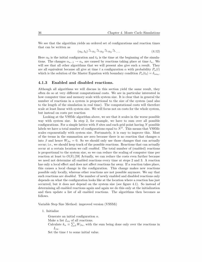
36 Chapter 4. Monte Carlo Simulations
We see that the algorithm yields an ordered set of configurations and reaction timesthat can be written as
(α0, t0)t1→α1
t2→α2t3→α3
t4→ . . . (4.12)
Here α0 is the initial configuration and t0 is the time at the beginning of the simula-tions. The changes αn−1 → αn are caused by reactions taking place at time tn. Wewill see that all other algorithms that we will present also give such a result. Theyare all equivalent because all give at time t a configuration α with probability Pα(t)which is the solution of the Master Equation with boundary condition Pα(t0) = δαα0
.
4.1.3 Enabled and disabled reactions.
Although all algorithms we will discuss in this section yield the same result, theyoften do so at very different computational costs. We are in particular interested inhow computer time and memory scale with system size. It is clear that in general thenumber of reactions in a system is proportional to the size of the system (and alsoto the length of the simulation in real time). The computational costs will thereforescale at least linear with system size. We will focus not on costs for the whole system,but instead on costs per reaction
Looking at the VSSMc algorithm above, we see that it scales in the worse possibleway with system size. In step 2, for example, we have to sum over all possibleconfigurations. For a simple lattice with S sites and each grid point having N possiblelabels we have a total number of configurations equal to NS . This means that VSSMcscales exponentially with system size. Fortunately, it is easy to improve this. Mostof the terms in the summation are zero because there is no reaction that changes αinto β and hence Wβα = 0. So we should only use those changes that can actuallyoccur; i.e., we should keep track of the possible reactions. Reactions that can actuallyoccur at a certain location we call enabled . The total number of (enabled) reactionsis proportional to the system size, so we can reduce the scaling of computer time perreaction at least to O(S).[59] Actually, we can reduce the costs even further becausewe need not determine all enabled reactions every time at steps 2 and 3. A reactionhas only a local effect and does not affect reactions far away. If a reaction takes place,this causes a local change in the configuration. This change makes new reactionspossible only locally, whereas other reactions are not possible anymore. We say thatsuch reactions are disabled . The number of newly enabled and disabled reactions onlydepends on what the configuration looks like at the location where a reaction has justoccurred, but it does not depend on the system size (see figure 4.1). So instead ofdetermining all enabled reactions again and again we do this only at the initializationand then update a list of all enabled reactions. The algorithms then becomes asfollows.
Variable Step Size Method: improved version (VSSMi)
1. Initialize
Generate an initial configuration α.Make a list Lrx of all reactions.Calculate kα ≡
∑
β Wβα, with the sum being done only over the reactions inLrx.
Set the time t to some initial value.
4.1 Solving the Master Equation 37
O
O
CO
CO
O
O
CO
CO
O
O
CO
CO
O
CO
Figure 4.1: The left shows part of a configuration for a model of CO oxidation. The fatCO and oxygen form CO2 which is removed from the surface. The middle shows newlyenabled reaction; CO can adsorb at the sites marked by dark grey circles, oxygen canadsorb dissociatively on neighboring sites indicated by two light grey circles on theline connecting the sites. The right indicates a disabled reaction; the two encircledsites had a CO and an oxygen that could form a CO2.
Choose conditions when to stop the simulation.
2. Reaction time
Generate a time interval ∆t when no reaction takes place
∆t = − 1
kαln r, (4.13)
where r is a random deviate on the unit interval.Change time to t → t + ∆t.
3. Reaction
Pick the reaction α → α′ from Lrx with probability Wα′α/kα: i.e., do thereaction α → α′.
4. Update
Remove the reaction α → α′ from Lrx.Add new enabled reactions to Lrx and remove disabled reactions.Use these reactions to calculate kα′ from kα.
5. Continuation
If the stop conditions are fulfilled then stop. If not repeat at step 2.
The reasoning leading to VSSMi suggests that the computer time per reaction ofthis algorithm does not depend on system size. However, that is still not true. Thereare two problems. First, picking the reaction in step 3 cannot be done in constanttime just with the list of all reactions. Second, adding new enabled reactions to thelist of reactions can be done easily in constant time, but removing disabled reactionspresents a problem. One can scan the list of all reactions and in remove all disabledreactions from the list, but that is an O(S) operation. It may be possible to makelinks from the sites where the last reaction has occurred to the places in the list of allreactions where the possible disabled reactions reside, but that is very complicatedand has never been done.
38 Chapter 4. Monte Carlo Simulations
4.1.4 Weighted and uniform selection.
The selection in step 3 is a weighted selection. To make this selection one has todefine cumulative rate constants Cα′α ≡ ∑
β≤α′ Wβα′ . The configurations that canbe reached by a reaction from α need to be ordered, and the summation is over allconfigurations preceding α′ (β < α′) and α′ itself. The reaction α → α′ can thenbe picked by choosing α′ using Cα′−1α < rkα ≤ Cα′α where r is a random deviateon the unit interval and α′ − 1 is the configuration before α′ in the ordering of theconfigurations. This weighted selection scales linearly with the number of reactions;i.e., it scales as O(S). The reason for this is that we have to scan all the cumulativerate constants Cα′α.
To pick a reaction in constant time we split the list of all reactions in groupscontaining reactions of the same type (or more general with the same rate constant).Two reactions are of the same type if they differ only in their position and/or orienta-tion. So CO adsorption, NO dissociation (NO → N+O and N2 associative desorption
(2N → N2) are examples of reactions types. If L(i)rx is the list of N (i) reactions with
rate constant W (i), then we proceed as follows. First, we pick a type of reaction j
with probability N (j)W (j)/∑
i N (i)W (i), and then we pick from L(j)rx a reaction at
random. The first part scales linearly with the number of lists L(i)rx , because it is a
weighted selection. This number does not depend on the system size. The secondpart is a uniform selection, and can be done in constant time. So the second part alsodoes not depend on the system size. If the number of reaction types is small, and itoften is, this method is very efficient (see figure 4.2).
It is possible to do the weighted selection of the reactions also in O(log S) timeby using a binary tree.[59] Each node of the tree has a reaction and the cumulativerate constant of all reactions of the node and both branches below the node. Afterrkα has been determined we look for the node with Cleft < rkα ≤ Cleft +Wnode whereWnode is the rate constant of the reaction of the node and Cleft is the cumulative rateconstant of the top node of the left branch. If there is no left branch then we defineCleft = 0. To find the node we do we do the following.
1. Start
Set X = rkα.Take the top node of the tree.
2. Reaction found?
if Cleft < X ≤ Cleft + Wnode
then stop; take the reaction of the node.else go to the next step
3. Continue in the left branch?
if X ≤ Cleft
then take the top node of the left branch and continue at step 2else go to the next step
4. Continue in the right branch.
Set X → X − (Cleft + Wnode).Take the top node of the right branch and continue at step 2.
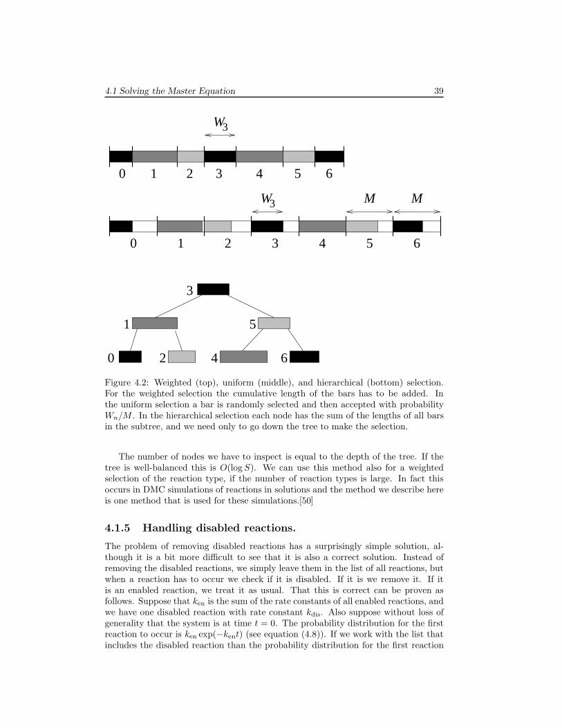
4.1 Solving the Master Equation 39
0 1 2 3 4 5 6
0 1 2 3 4 5 6
0 2 4 6
51
3
3W
3W MM
Figure 4.2: Weighted (top), uniform (middle), and hierarchical (bottom) selection.For the weighted selection the cumulative length of the bars has to be added. Inthe uniform selection a bar is randomly selected and then accepted with probabilityWn/M . In the hierarchical selection each node has the sum of the lengths of all barsin the subtree, and we need only to go down the tree to make the selection.
The number of nodes we have to inspect is equal to the depth of the tree. If thetree is well-balanced this is O(log S). We can use this method also for a weightedselection of the reaction type, if the number of reaction types is large. In fact thisoccurs in DMC simulations of reactions in solutions and the method we describe hereis one method that is used for these simulations.[50]
4.1.5 Handling disabled reactions.
The problem of removing disabled reactions has a surprisingly simple solution, al-though it is a bit more difficult to see that it is also a correct solution. Instead ofremoving the disabled reactions, we simply leave them in the list of all reactions, butwhen a reaction has to occur we check if it is disabled. If it is we remove it. If itis an enabled reaction, we treat it as usual. That this is correct can be proven asfollows. Suppose that ken is the sum of the rate constants of all enabled reactions, andwe have one disabled reaction with rate constant kdis. Also suppose without loss ofgenerality that the system is at time t = 0. The probability distribution for the firstreaction to occur is ken exp(−kent) (see equation (4.8)). If we work with the list thatincludes the disabled reaction than the probability distribution for the first reaction
40 Chapter 4. Monte Carlo Simulations
occurring at time t being also an enabled reaction is ken exp(−(ken + kdis)t), whichis the probability that no reaction occurs until time t and then an enabled reactionoccurs. This is the first contribution to the probability distribution for the enabledreaction if the disabled reaction is not removed. The probability distribution that thefirst reaction is not but the second reaction is enabled and occurs at time t is givenby
ken
∫ t
0
dt′ e−ken(t−t′)kdise−(ken+kdis)t
′
= kene−kentkdis
∫ t
0
dt′ e−kdist′
= kene−kent[
1 − e−kdist]
. (4.14)
Adding this to ken exp(−(ken+kdis)t) gives us ken exp(−kent), which is what we shouldhave.
This shows that adding a single disabled reaction does not change the probabilitydistribution for the time that the first enabled reaction occurs. In the same way we canshow that adding a second disabled reaction gives the same probability distributionas having a single disabled reaction, and that adding a third disabled reaction is thesame as having two disabled reactions, etc. So by induction we see that disabledreactions do not change the probability distribution for the occurrence of the enabledreactions. Also step 3 of VSSMi is no problem. The enabled reactions are chosen witha probability proportional to their rate constant whether or not disabled reactions arepresent in he list.
The VSSM algorithm now gets the following form.
Variable Step Size Method with an approximate list of reactions (VSSMa)
1. Initialize
Generate an initial configuration α.
Make lists L(i)rx containing all reactions of type i.
Calculate k(i) ≡ N (i)W (i), with N (i) the number of reactions of type i andW (i) the rate constant of these reactions.
Set the time t to some initial value.Choose conditions when to stop the simulation.
2. Reaction time
Generate a time interval ∆t when no reaction takes place
∆t = − 1∑
i k(i)ln r, (4.15)
where r is a random deviate on the unit interval.Change time to t → t + ∆t.
3. Reaction
Pick a type of reaction j with probability k(j)/∑
i k(i), and then pick the
reaction β → α′ from L(j)rx at random. If the reaction is enabled go to
step 4. If it is disabled go to step 6. (Note that during the simulationk(j) may have obtained contributions from disabled reactions starting fromconfigurations different from α.)
4.1 Solving the Master Equation 41
4. Enabled reaction
Change the configuration to α′.
5. Enabled update
Remove the reaction β → α′ from L(j)rx . Change k(j) → k(j) − W (j). (Note
that because the reaction is enabled β = α.)
Add new enabled reactions to the lists L(i)rx .
Use these reactions to calculate the new values for k(i) from the old ones.Skip to step 8.
6. Disabled reaction
Do not change the configuration; α′ is the same configuration as α.
7. Disabled update
Remove the disabled reaction from L(j)rx .
Change k(j) → k(j) − W (j).
8. Continuation
If the stop conditions are fulfilled then stop. If not repeat at step 2.
The computer time per reaction of algorithm VSSMa scales as O(1). This isachieved by working with an approximate list of all reactions; a list that can containdisabled reactions. We will see that the same trick can be used with other algorithmsas well. Note that picking the reaction type at step 3 can be done hierarchically asexplained at the end of section 4.1.4.
4.1.6 Reducing memory requirements.
There are other ways we might want to change the VSSM algorithm, but then becauseof memory considerations. The description of the algorithms uses a list of all reactions.This list is quite large and scales with system size. We can do away with this list atthe cost of increasing computer time, although the algorithm will still scale as O(1).
Instead of keeping track of all individual reactions we only keep track of how many
reactions there are of each different type; i.e., no lists L(i)rx but only the numbers N (i).
Because there are no lists we have to count how many reactions become disabled aftera reaction has occurred. This is similar to adding enabled reactions and can be donein constant time. (Note that this is only because we are using no lists. Removingdisabled reactions from lists is what costs time.) This means that the number N (i)
will be exact. The only problem is, after the type of reaction is determined, how todetermine which particular reaction will take place. This can be done by randomlysearching on the surface. The number of places one has to look does not depend onthe system size, but on the probability that the reaction can occur on a randomlyselected site. This random search for the location of the reaction is another form ofuniform selection. Another application of such a uniform selection will be given insection 4.1.9. If the type of reaction can take place on many places, then a particularreaction should rapidly be found.
To make the formulation of the new algorithm not too difficult we use a morerestrictive definition of a reaction type, in the sense that two reactions are of thesame type if one can be obtained from to other by a translation. Previously we alsotalked about the same reaction type if the orientation was different. We don’t do this
42 Chapter 4. Monte Carlo Simulations
here, because we want to have an unambiguous meaning if we say that a reactionoccurs at a particular site (see step 4 of VSSMs) even if more sites are involved. Forexample, if we have a reaction type of an A reacting with a B where the B is at a siteto the right of the A, then by the site of this reaction we mean the site where the Ais. The new algorithm then becomes as follows.
Variable Step Size Method with random search for the location of reactions (VSSMs).
1. Initialize
Generate an initial configuration.Count how many reactions N (i) of type i there are.Calculate k(i) ≡ N (i)W (i), with W (i) the rate constant of the reactions of type
i.Set the time t to some initial value.Choose conditions when to stop the simulation.
2. Reaction time
Generate a time interval ∆t when no reaction takes place
∆t = − 1∑
i k(i)ln r, (4.16)
where r is a random deviate on the unit interval.Change time to t → t + ∆t.
3. Reaction type
Pick a type of reaction j with probability k(j)/∑
i k(i).
4. Reaction location
Pick randomly a site for the reaction, until a site is found where the reactioncan actually occur.
5. Update
Change the configuration.Determine the new enabled reactions, and change the N (i)’s accordingly.Determine the disabled reactions, and change the N (i)’s accordingly.
6. Continuation
If the stop conditions are fulfilled then stop. If not repeat at step 2.
4.1.7 Oversampling and the Random Selection Method.
The determination of a reaction and its time can be split in three parts; the time ofthe reaction, the type of the reaction, and the site of the reaction. The last two partswere combined in the previous versions of VSSM. The determination of the reactiontype has to be done before the determination of the location of the reactions in VSSMs(otherwise one doesn’t know when to stop searching in step 4), but the time of thereaction can be determined independently from which reactions occurs where. It isalso possible to determine all three parts independently. This has the advantage thateven less bookkeeping is necessary; adding and removing reactions to update lists ornumbers of types of reaction is not necessary. The drawback is however the same as
4.1 Solving the Master Equation 43
in VSSMs, only worse; as in step 4 of VSSMs reactions will be attempted at certainlocations where the reactions cannot take place. If this does not occur to often, thenthis drawback may be small.
The trick to do away with the bookkeeping is to use a technique called oversam-
pling. Suppose we have just one type of reaction and that we have N of them. (Areaction type is defined here in the same way as for VSSMs.) The time to the nextoccurrence of a reaction is then given the probability distribution NW exp(−NWt)where W is the rate constant of the reaction. If we assume, however, that we haveM of these reactions with M > N then we can also generate the time of the nextreaction from the distribution MW exp(−MWt), but then accept the reaction withprobability N/M . To prove this we need to add the contributions that the reactionhas to be generated one, two, three etc. times before one is found that is accepted.
N
MMW exp(MWt)
+
∫ t
0
dt′N
MMWe−MW (t−t′)
[
1 − N
M
]
MWe−MWt′
+
∫ t
0
dt′∫ t′
0
dt′′N
MMWe−MW (t−t′)
×[
1 − N
M
]
MWe−MW (t′−t′′)
[
1 − N
M
]
MWe−MWt′′ + . . .
= NWe−MWt
[
1 +
[
1 − N
M
]
MWt +1
2
[
1 − N
M
]2
M2W 2t2 + . . .
]
= NWe−MWte[1−N/M ]MWt = NWe−NWt. (4.17)
The following algorithm is only useful if we do not need to determine N explic-itly. This can be accomplished if we assume that all reaction types can take place
everywhere on the surface. In terms of lists this means that each list L(i)rx has the
same S reactions during an entire simulation. Because the lists do not change andthey have a simple definition, we do not need to determine them explicitly. Also thetimes of the reactions are always taken from the same probability distribution, andthe probabilities to choose a reaction type do not change. The algorithm looks asfollows.
Random Selection Method (RSM).
1. Initialize
Generate an initial configuration.Set the time t to some initial value.Define k ≡ SWmax where Wmax is the maximum of the rate constants W (i)’s
of type i.Choose conditions when to stop the simulation.
2. Reaction time
Generate a time interval ∆t when no reaction takes place
∆t = −1
kln r, (4.18)
44 Chapter 4. Monte Carlo Simulations
where r is a random deviate on the unit interval.
3. Reaction type
Pick a type of reaction randomly.
4. Reaction location
Pick a site randomly.
5. Update
Change time to t → t + ∆t.If the reaction is possible at the site from step 4, then accept the reaction with
probability W (i)/Wmax where i is the type of reaction from step 3If the reaction is possible and accepted, change the configuration.
6. Continuation
If the stop conditions are fulfilled then stop. If not repeat at step 2.
This algorithm is called the Random Selection Method (RSM). Note that thereaction time, the type of the reaction, and the location of the reaction can be donein any order. Only time and the configuration of the system needs to be updated.The method is therefore very efficient, provided that in step 5 reaction are acceptedoften.
4.1.8 The First Reaction Method.
Instead of splitting the time, the type, and the location of a reaction, it is also possibleto combine them. This is done in the First Reaction Method.
The First Reaction Method (FRM)
1. Initialize
Generate an initial configuration α.Set the time t to some initial value.Make a list Lrx containing all reactions.Generate for each reaction α → β in Lrx a time of occurrence
tβα = t − 1
Wβαln r (4.19)
with Wβα the rate constant for the reaction and r a random deviate onthe unit interval.
Choose conditions when to stop the simulation.
2. Reaction
Take the reaction α → α′ with tα′α ≤ tβα for all β.If the reaction is enabled go to step 3. If not go to step 4.
3. Enabled update
Change the configuration to α′.Change time to t → tα′α
Remove the reaction α → α′ from Lrx.
4.1 Solving the Master Equation 45
Add new enabled reactions to Lrx and generate for each reaction α′ → β atime of occurrence
tβα′ = t − 1
Wβα′
ln r. (4.20)
Skip to step 5.
4. Disabled update
Do not change the configuration: α′ is the same configuration as α.Remove the disabled reaction from Lrx.
5. Continuation
If the stop conditions are fulfilled then stop. If not set α to α′ and repeat atstep 2.
This algorithm is called Discrete Event simulation in computer science.[60] InFRM the determination of the type and the site of a reaction is replaced by compar-ing times of occurrences for individual reactions. That this is correct can be seen asfollows. Suppose we have two reactions with rate constants W1 and W2. The proba-bility that no reaction occurs in the interval [0, t] is then exp[−(W1 + W2)t], whereasthe probability that neither reaction 1 nor reaction 2 occurs in that interval equalsexp(−W1t) exp(−W2t), which is obviously the same as the previous expression. Thisproves that FRM generates correct reaction times. It’s a bit more work to show thatthe reactions are chosen with the correct probability. The probability distribution forthe reactions times of the reactions are Wi exp(−Wit) with i = 1, 2. The probabilitythat reaction 1 occurs before reaction 2 in the FRM algorithm is given by
∫ ∞
0
dt W1e−W1t
∫ ∞
t
dt′W2e−W1t′ (4.21)
= W1
∫ ∞
0
dt e−W1te−W2t =W1
W1 + W2.
For reaction 2 we find W2/(W1 +W2), which shows that FRM also picks the reactionswith the correct probability. So we see that one can either generate one time for allreactions and then choose one reaction, or generate times for all reactions and thentake the first that will occur. We will use this later on in another way.
The disadvantage of FRM is the determination of the reaction with the smallesttime of occurrence. Scanning a list of all reaction for each new reaction scales as O(S).More efficient is to make the list of all reactions an ordered one, and keep it orderedduring a simulation. Getting the next reaction scales then as O(1), but inserting newreactions in Lrx scales as O(log S).[59] This is not as good as constant time, but it isnot particularly bad either. Still VSSM is often more efficient than FRM, but VSSMcannot always be used as we will show later, whereas FRM can always be used.
Note that disabled reactions are not removed from the list of all reactions. Notealso that we only have to generate reaction times for the new enabled reactions.Times for reactions already in Lrx need not be generated again. Suppose that attime t = t1 a time has been generated for a reaction with rate constant W . Theprobability distribution for that time is W exp[−W (t− t1)]. Now assume that at timet = t2 > t1 the reaction has not occurred. We might generate a new time using the newprobability distribution W exp[−W (t− t2)]. However, the ratio of the values of theseprobability distributions for times t > t2 is W exp[−W (t− t2)]/W exp[−W (t− t1)] =
46 Chapter 4. Monte Carlo Simulations
exp[W (t2 − t1)] is a constant. Hence relative probabilities for the times t > t2 thatthe reaction can occur are the same for both probability distributions, and no newtime need to be generated.
4.1.9 Practical considerations
There are different aspects to consider by people who just want to use the algorithmsabove to simulate a particular reactions system, and by people who want to implementthem. For the implementation the efficiency of the methods described above dependsvery much on details of the algorithm that we have not discussed. However, somegeneral guidelines can and will be given here. The interested reader is referred toreferences [61] and [62] for a more extensive analysis.
An important point is that memory and computation time depend mainly on thedata structures that are used. Except for the time steps there is relatively little toreally calculate. This involves the generation of a random number. Random numbersare also needed to pick reactions or reaction types and sites. More critical are the datastructures that contain the reactions and/or reaction types. These lists are priorityqueues,[59] and in particular for FRM these may become quite large. A problem arethe disabled reactions. Removing them depends linearly on the size of the lists and isgenerally inefficient, and should not be done after each reaction. It is better to removethem only when they should occur, and it is found that they have become disabled.Alternatively, one can do garbage collection when the size of the list becomes toolarge.[63] The determination of the next reaction that should occur depends onlylogarithmically on the size of the list in FRM. In VSSM and RSM this can even bedone in constant time.
There are a few other aspects that are important and that we haven’t mentionedyet. A central step in all algorithms is the determination of what are the new reactionsthat have become possible just after a reaction has occurred. There are dependenciesbetween the reactions that may be used to speed up the simulation. A small examplemay make this clearer. Suppose we have just adsorption of A or B onto vacant sites,and formation of AB from an A next to a B leaving two vacant sites. The formationof an AB will allow new A and B adsorptions, but no new AB formation. So it is notnecessary to check if any AB formations have become enabled.
Testing if a reaction is disabled is not trivial. It won’t do to see if the occupationof the relevant sites allows the reaction to occur. It may be that the occupation ofthe sites has changed a few times but then converted back to a situation so that thereaction can occur again. What has happened then is that when the reaction becameenabled for the second time it was added to the list of reactions for the second timetoo. If the first instance of the reaction on the list is not recognized as disabled,then the reaction will take place at the first time of occurrence. This means thateffectively the reaction has a double rate constant. This is similar to oversampling(section 4.1.7) and accepting each reaction with probability 1. (This problem doesnot occur, of course, in VSSMs and in RSM.)
Recognizing that a reaction is disabled can be done by keeping track of when areaction became enabled and when the occupation of a site last changed. If a siteinvolved in the reaction changed after the reaction became enabled, then the reactionshould be regarded as being disabled. Using the times of these changes may howeverlead to problems because of rounding errors in the representation of real (floating
4.1 Solving the Master Equation 47
point) numbers. Instead one can use integers that count reactions when they becomeenabled. Each reaction is assigned then its count number, and each site is assignedthe number of the reaction that last changed it. It a site involved in a reaction has anumber larger than the number of the reaction, then the reaction is disabled.
From the point of view of using the algorithms to simulate a system an importantaspect seems to be the scaling with system size. The important difference betweenFRM on the one, and VSSM (i.e., VSSMa and VSSMs) and RSM on the other handis the dependence on the system size. Computer time per reaction in VSSM and RSMdoes not depend on the size of the system. This is because in these methods pickinga reaction is done using uniform selection, which does not depend on the size of thelist of reactions. In RSM there is not even such a list. In FRM the computer time perreaction depends logarithmically on the system size. Here we have to determine whichof all reactions will occur first. So for large systems VSSM and RSM are generallyto be preferred. The data structure of FRM is so time consuming that FRM shouldonly be used if really necessary.
There are however a number of cases that occur quite frequently in which VSSMand RSM are not efficient. This is when there are many reaction types and whenthe rate constants depend on time. Time-dependent rate constants will be discussedin section 4.1.10. Many reaction types arise, for example, when there are lateralinteractions. In this case VSSM becomes inefficient because it will take a lot of timeto determine the reaction type. If with the lateral interactions many adsorbates affectthe rate constant of a reaction, then the number of reaction types easily becomes largerthan the number of sites (see section 5.7). RSM can be used for lateral interactions,provided that the effect of them is small. With RSM one need only include in thereaction description those sites for which the occupancy changes. If one also includesthe sites with the adsorbates affecting the rate constants then the probability thatone picks a reaction type that can occur at the randomly chosen site is too low.The adsorbates affecting the rate constants should, of course, be included when onecalculates the rate constant for the determination of the acceptance of a reaction. Ifthe effect of lateral interactions is large then this acceptance will often be low, andRSM will not be very efficient. This is very often the case. In general, one shouldrealize that simulations of systems with lateral interactions are always costly.
If VSSM and RSM can be used, then the choice between them depends on howmany sites in the system the reactions can occur. RSM is efficient for reactions thatoccur on many sites. The probability that a reaction is possible on the randomlychosen location is then high. If this is not the case then VSSM should be used.
The choice between FRM, VSSM, and RSM need not be made for all reactionsin a system together, but can be made on a per reaction type basis, because it iseasy to combine the different methods. Suppose that reaction type 1 is best treatedby VSSM, but reaction type 2 best by RSM. We then determine the first reaction oftype 1 using VSSM, and the first of type 2 by RSM. The first reaction to actuallyoccur is then simply the first reaction of these two. The proof that this is correct isidentical to the proof of the correctness of FRM. Combining algorithms in this waycan be particularly advantageous for models with many reaction types.
To summarize, VSSM is generally the best method to use unless the number ofreaction types is very large. In that case use FRM. If you have a reaction thatoccurs almost everywhere, RSM should be considered. Simply doing the simulationwith different methods and comparing is of course best. One should also look for
48 Chapter 4. Monte Carlo Simulations
alternative ways to model the system (see chapter 5).
4.1.10 Time-dependent transition probabilities.
If the transition probabilities Wαβ are themselves time dependent, then the integralformulation above needs to be adapted. This situation arises, for example, whendealing with Temperature-Programmed Desorption or Reactions (TPD/TPR),[43, 64,65] and when dealing with voltammetry.[66] The definition of the matrices W and Rremains the same, but instead of a matrix Q(t) we get
Q(t′, t) ≡ exp
[
−∫ t′
t
dt′′ R(t′′)
]
. (4.22)
With this new Q matrix the integral formulation of the Master Equation becomes
P(t) =
[
Q(t, 0) +
∫ t
0
dt′Q(t, t′)W(t′)Q(t′, 0) (4.23)
+
∫ t
0
dt′∫ t′
0
dt′′Q(t, t′)W(t′)Q(t′, t′′)W(t′′)Q(t′′, 0) + . . .
]
P(0).
The interpretation of this equation is the same as that of equation (4.6). This meansthat it is also possible to use VSSM to solve the Master Equation. The relevantequation to determine the times of the reactions becomes
Q(tn, tn−1) = r, (4.24)
where tn−1 is the time of the last reaction that has occurred, and the equation shouldbe solved for tn, which is the time of the next reaction. If just after tn−1 the systemis in configuration αn−1, then the next reaction leading to configuration αn shouldbe picked out off all possible reaction with probability proportional to Wαnαn−1
(tn).The drawback of VSSM for time-dependent transition probabilities is that the
equation for the times of the reactions is often very difficult to be solved efficiently.Equation (4.24) can in general not be solved analytically, but a numerical solutionwith a Q of the form shown in figure 4.3 is also not easy. The problem is that Rin equation (4.22) can contain many terms or terms that have a very different timedependence due to reactions with different activation energy. A possible solution isto use VSSM for each reaction type separately; i.e., we solve equation (4.24) for eachreaction type separately. The next reaction is then of the type with the smallest valuefor tn, and the first reaction is chosen from those of that type as in VSSM.[62] Thisworks provided the number of reaction types is small.
Instead of computing a time for the next reaction using the sum of the transitionprobabilities of all possible reactions, we can also compute a time for each reaction. Soif we’re currently at time t and in configuration α, then we compute for each reactionα → β a time tβα using
exp
[
−∫ tβα
t
dt′ Wβα(t′)
]
= r, (4.25)
where r is again a uniform deviate on the unit interval. The first reaction to occuris then the one with the smallest tβα. It can be shown that this time has the same
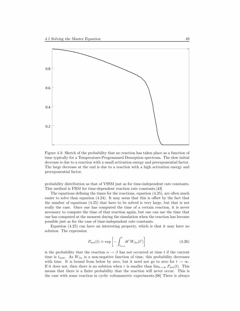
4.1 Solving the Master Equation 49
0.2
0.4
0.6
0.8
Figure 4.3: Sketch of the probability that no reaction has taken place as a function oftime typically for a Temperature-Programmed Desorption spectrum. The slow initialdecrease is due to a reaction with a small activation energy and preexponential factor.The large decrease at the end is due to a reaction with a high activation energy andpreexponential factor.
probability distribution as that of VSSM just as for time-independent rate constants.This method is FRM for time-dependent reaction rate constants.[43]
The equations defining the times for the reactions, equation (4.25), are often mucheasier to solve than equation (4.24). It may seem that this is offset by the fact thatthe number of equations (4.25) that have to be solved is very large, but that is notreally the case. Once one has computed the time of a certain reaction, it is nevernecessary to compute the time of that reaction again, but one can use the time thatone has computed at the moment during the simulation when the reaction has becomepossible just as for the case of time-independent rate constants.
Equation (4.25) can have an interesting property, which is that it may have nosolution. The expression
Pnot(t) ≡ exp
[
−∫ t
tnow
dt′ Wβα(t′)
]
(4.26)
is the probability that the reaction α → β has not occurred at time t if the currenttime is tnow. As Wβα is a non-negative function of time, this probability decreaseswith time. It is bound from below by zero, but it need not go to zero for t → ∞.If it does not, then there is no solution when r is smaller than limt→∞ Pnot(t). Thismeans that there is a finite probability that the reaction will never occur. This isthe case with some reaction in cyclic voltammetric experiments.[66] There is always
50 Chapter 4. Monte Carlo Simulations
a solution if the integral goes to infinity. This is the case when Wβα goes slower tozero than 1/t, or does not go to zero at all.
4.2 A comparison with other methods.
There are a few other approaches that we want to mention here. The fixed timestep method discretized time. The algorithmic methods are older methods that arestill being used. Kinetic Monte Carlo is very similar to VSSM and is quite popular.Cellular Automata are mentioned also but only briefly, as they are really outside thescope of this introduction to MC methods.
4.2.1 The fixed time step method
If we discretize time then the Master Equation can be written as
Pα(t + ∆t) = Pα(t) +∑
β
[Wαβ∆t Pβ(t) − Wβα∆t Pα(t)] . (4.27)
This means that if at time t we are in configuration α, then at time t+∆t we are stillin configuration α with probability 1 −∑β Wβα∆t and in configuration β differentfrom α with probability Wβα∆t. This leads to the following algorithm. For eachreaction α → β we generate a random number between 0 and 1. If r ≤ Wβα∆t thenwe change the configuration to β and time to t + ∆t. If r > Wβα∆t then we onlychange time to t + ∆t.
The algorithm above can be very efficient if it works. For example, if the rateconstants are time dependent, then the fixed time step method assumes that it isconstant during the interval [t, t + ∆t]. This avoids the evaluation of integrals like(4.25). However, it is obviously an approximation, which might necessitate smalltime steps. The time step also has to be small because the probabilities Wβα∆t and1 −∑β Wβα∆t must be between 0 and 1. Determining the maximum ∆t that givescorrect results might be cumbersome.
A more subtle problem is that one should avoid the possibility that two reactionscannot both occur but for both holds r ≤ Wβα∆t. For example, an adsorbate candesorb or react with a neighbor. The adsorbate cannot do both, but if for bothreactions we find r ≤ Wβα∆t, then we have a problem. In practice this means that∆t should be chosen so small that at most one reaction occurs during each time step.
4.2.2 Algorithmic approach
Almost all older Dynamic Monte Carlo methods are based on an algorithm that definesin what way the configuration changes. (A nice review with many references to workwith these methods is reference [67].) The generic form of that algorithm consistsof two steps. The first step is to pick a site. The second step is to try all reactionsat that site. (This may involve picking additional neighboring sites.) If a reaction ispossible at that site, then it is executed with some probability that is characteristicfor that reaction. These two steps are repeated many times. The sites are generallypicked at random. In a variant of this algorithm just one reaction is tried until onaverage all sites have been visited once, and then the next reaction is tried, etc. Thisvariant is particular popular in situations with fast diffusion; the “real” reactions are
4.2 A comparison with other methods. 51
tried first on average once on all sites, and then diffusion is used to equilibrate thesystem before the next cycle of “real” reactions.
These algorithmic Dynamic Monte Carlo methods have provided very valuableinsight in the way the configuration of the adsorbates on a catalyst evolves, but theyhave some drawbacks. First of all there is no real time. Instead time is specifiedin so-called Monte Carlo steps (MCS). One MCS is usually defined as the cycle inwhich every site has on average been visited once for each reaction. The seconddrawback is how to choose the probabilities for reactions to occur. It is clear thatfaster reactions should have a higher probability, but it is not clear how to quantifythis. This drawback is related to the first. Without a link between these probabilitiesand microscopic reaction rate constants it is not possible a priori to tell how manyreal seconds one MCS corresponds to. The idea is that Monte Carlo time in MCSand real time are proportional. We have used the similarity with RSM and shownthat this is indeed the case provided temporal fluctuations are disregarded and onehas a steady state. In the case of, for example, oscillations the two time scales arenot proportional.[61] In practice people have used the algorithmic approach to lookfor qualitative changes in the behavior of the system when the reaction probabilitiesare varied, or they have fitted the probabilities to reproduce experimental results.
The third drawback is that it is difficult with this algorithmic definition to comparewith other kinetic theories. Of course, it is possible to compare results, but an analysisof discrepancies in the results is not possible as a common ground (e.g., the MasterEquation in our approach) is missing. The generic form of the algorithm describedabove resembles the algorithm of RSM. Indeed one may look upon RSM as a methodin which the drawbacks of the algorithmic approach have been removed.
4.2.3 Kinetic Monte Carlo
The problem of real time in the algorithmic formulation of Dynamic Monte Carlo hasalso been solved by Fichthorn and Weinberg.[54] Their method is called Kinetic MonteCarlo (KMC) and has become quite popular. They replaced the reaction probabilitiesby rate constants, and assumed that the probability distribution Prx(t) of the timethat a reaction occurs is a Poisson process; i.e., it is given by
Prx(t) = k exp[−k(t − tnow)], (4.28)
where tnow is the current time, and k is the rate constant. Using the properties ofthis distribution they derived a method that is really identical to our VSSM, expectin two aspects. One aspect is that the Master Equation is absent, which makes itagain difficult to make a comparison with other kinetic theories. Instead the methodwas derived by asking under which conditions an equilibrium MC simulation can beinterpreted as a temporal evolution of a system. The other aspect is that time is incre-mented deterministically using the expectation value of the probability distributionof the first reaction to occur; i.e.,
∆t =1
∑
i Niki, (4.29)
where ki is the rate constant of reaction type i (this is the same as our transitionprobabilities W in equation (2.4)), and Ni is the number of reaction of type i. Thisavoids having to solve equation (4.10), and has been used subsequently by many
52 Chapter 4. Monte Carlo Simulations
others. However, as solving that equation only involves generating a random numberand a logarithm, which is a negligible contribution to the computer time, this is notreally an advantage. Equation (4.29) does neglect temporal fluctuations, which maybe incorrect for systems of low dimensionality.[68]
Although the derivation of Fichthorn and Weinberg only holds for Poisson pro-cesses, their method has also been used to simulate TPD spectra.[56] In that workit was assumed that, when ∆t computed with equation (4.29) is small, the rate con-stants are well approximated over the interval ∆t by their values at the start of thatinterval. This seems plausible, but, as the rate constants increase with time in TPD,equation (4.29) systematically overestimates ∆t, and the peaks in the simulated spec-tra are shifted to higher temperatures. In general, if the rate constants are timedependent then it may not even be possible to define the expectation value. We havealready mentioned the case of cyclic voltammetry where there is a finite probabilitythat a reaction will not occur at all. The expectation value is then certainly notdefined. Even if a reaction will occur sooner or later the distribution Prx(t) has to gofaster to zero for t → ∞ than 1/t2 for the expectation value to be defined. Solvingequations (4.10) or (4.25) does not lead to such problems.
4.2.4 Cellular Automata
There is an extensive literature on Cellular Automata. A discussion of this is outsidethe scope of this chapter, and we will restrict ourselves to some general remarks. Wewill also restrict ourselves to Cellular Automata in which each cell corresponds toone site. The interested reader is referred to references[69, 70, 71, 72, 73, 74] for anoverview of the application of Cellular Automata to surface reactions.
The main characteristic of Cellular Automata is that each cell, which correspondsto a grid point in our model of the surface, is updated simultaneously. This allows foran efficient implementation on massive parallel computers. It also facilitates the simu-lation of pattern formation, which is much harder to simulate with some asynchronousupdating scheme as in Dynamic Monte Carlo.[75] The question is how realistic a si-multaneous update is, as a reaction seems to be a stochastic process. One has triedto incorporate this randomness by using so-called probabilistic Cellular Automata, inwhich updates are done with some probability. These Cellular Automata differ littlefrom Dynamic Monte Carlo. In fact, probabilistic Cellular Automata can be madethat are equivalent to the RSM algorithm.[62]
4.3 The CARLOS program
CARLOS is a general purpose program for surface reactions.[76] It was developedby Johan Lukkien at the Eindhoven University of Technology in the Netherlands.General purpose means that it does not have any reaction hard-coded, but one canspecify almost any type of reaction on input. For time-independent rate constants onecan choose between VSSM, RSM, and FRM. With time-independent rate constantsthe different methods can be combined in one simulation. For time-dependent rateconstants only FRM can be used. Each rate constant W can be specified as a constantor as
W = νe−Eact/kBT , (4.30)
4.3 The CARLOS program 53
and the preexponential factor ν, the activation energy Eact, and the temperatureT are to be given on input. These quantities can be linear functions of time. Inthis way one can simulate TPD/TPR experiments (T a function of time) and linearsweep voltammetry experiments (Eact a function of time). One can also change anyquantity in discrete steps. This allows the use of VSSM and RSM for rate constantswith arbitrary time dependence, although strictly speaking only approximately.
CARLOS uses pattern recognition for finding which reactions are possible. Eachreaction has to be specified as a list of sites involved in the reaction, the occupationof the sites before, and the occupations of them after the reaction has taken place.For example, in
(0, 0), (1, 0) : A B → ∗ ∗ (4.31)
an integer pair (n1, n2) indicates a unit cell, A and B are reactions, and ∗ the product.This can be interpreted as an molecule A reacting with a molecule B at a neighboringsite to form AB which immediately desorbs leaving two vacant sites. This interpreta-tion, however, is based on the meaning of the labels A, B, and ∗. CARLOS does notknow this meaning so the interpretation is ultimately up to the user. CARLOS onlysearches for a pattern on the left of the arrow and changes it to the pattern on theright. The labels can also be used to indicate different substrate atoms, types of sites(sites with different coordination numbers, defect sites, step sites, etc.), or surfacereconstruction.
The indices specifying the unit cells are relative. The specification above standsnot just for a reaction at (0, 0) and (1, 0), but at (n1, n2) and (n1 + 1, n2) for anyintegers n1 and n2. Having more than one site per unit cell is also possible. Forexample in
(0, 0/0), (0, 0/1) : A B → ∗ ∗ (4.32)
the reaction takes place on two sites in the same unit cell. The integers after theslash indicate which sites are involved. CARLOS does not make any assumptions ondistances or angles. So
(0, 0), (1, 0) : A B → ∗ ∗ (4.33)
may refer to a square, a hexagonal, or any other type of lattice. However, to simplifythe specification of many symmetry related reactions, one can specify this symmetry,and then CARLOS does assume certain conventions in the specification of the sites.For example, the lines
Active sites: top on hex...
...Symmetry: hex 120
. . . (0, 0), (1, 0) : A B → ∗ ∗on input make CARLOS assume that the lattice is hexagonal, and that the primitivetranslation vectors have the same length and make an angle of 60. Apart from thereaction explicitly stated above, CARLOS will also generate
(0, 0), (−1, 1) : A B → ∗ ∗ (4.34)
and
(0, 0), (0,−1) : A B → ∗ ∗, (4.35)
which are obtained by rotations of 120.
54 Chapter 4. Monte Carlo Simulations
As output CARLOS can generate a list of coverages and rates as a function oftime. This list contains all possible information on the kinetics. The configuration ofa system as a function of time can be shown on screen and/or sent to a file either ingraphic format or in a format that CARLOS can use to start a new simulation.
CARLOS always produces output concerning the performance of itself. This in-cludes how long it took to do a simulation, but also information on the efficiencywith which each type of reaction was simulated. This information can then be usedto change the method, or to change the way a reaction system is modeled. The ef-ficiency can also be influenced through CARLOS’s garbage collection that removesdisabled reactions. One can specify how much memory CARLOS should use. Thismakes it possible to run CARLOS with limited computer resources, but it can also beused to increase the frequency with which CARLOS does garbage collection. CAR-LOS also has an option that tries to optimize its memory usage. CARLOS does nothave any hard coded limits on the number of reactants, the number of reaction types,or the system size. This depends only on computer limits.
A special class of reactions are formed by the so-called immediate reactions. Theytake place as soon as they become enabled; time is not advanced. These reactionswere originally introduced to simulate models with infinitely fast reactions like theCO2 formation in the ZGB-model. They proved to be also very useful, however,for making efficient models of other reaction systems. CARLOS distinguishes evenimmediate reactions with different priorities; reactions with higher priorities takeplace before immediate reactions with lower priorities.
One common application of these immediate reactions is repulsive interactionsthat are so strong that they are always avoided by a system. Suppose that a moleculeA strongly repels other A’s on neighboring sites. Instead of implementing this strongrepulsion as a situation with high energy, it may be more efficient to block all neigh-boring sites of each A. This can be accomplished by an immediately reaction.
(0, 0), (1, 0) : A ∗ → A blocked (4.36)
where ∗ is a vacant site and “blocked” is also a vacant site, but one that cannot beoccupied by another adsorbate. We assume for simplicity that there is just one siteper unit cell, and that the other neighboring sites will be blocked by similar immediatereactions. Things become a bit complicated when the A is removed by, for example,a desorption. Using a normal reaction of the form
(0, 0), (1, 0) : A blocked → ∗ ∗ (4.37)
will not work. One reason is that this will change only one neighboring site from“blocked” to ∗. Another is that the neighboring site might have another A neighbor,so that it should remain blocked.
What does work are a normal reaction for the desorption and two immediatereactions to update the “blocked” labels. The desorption is specified by
(0, 0) : A → removed (4.38)
where “removed” specifies a vacant site where an A has been removed. This label isused to trigger the first new immediate reaction
(0, 0), (1, 0) : removed blocked → removed ∗. (4.39)
4.4 Dynamic Monte Carlo simulations of rate equations 55
After this reaction has changed all “blocked” labels of the neighboring sites a secondnew immediate reaction
(0, 0) : removed → ∗ (4.40)
removes it. This procedure may seem to have the same error that there might beanother A neighbor so that the site should retain the “blocked” label. However, thiscan be corrected if now the original immediate reaction (4.36) takes place again. Thisprocedure is correct provided that the immediate reactions are done in a certain order.Reaction (4.36) should have the lowest priority as it should occur last. Reaction (4.40)should have a higher priority, and reaction (4.39) should have the highest priority.Note that there is an obvious overhead; vacant sites with two or more neighboring A’swill change their label from “blocked” to ∗ and then immediately back to “blocked”again. This overhead is often negligible.
Lateral interactions can also be treated specially by CARLOS. Suppose that wehave a one-dimensional system with molecules A that only desorb. To include theinfluence of neighboring A’s one can specify desorption from all possible configurationsof an A and its neighboring sites. For a one-dimensional system this involves just fourconfiguration: ∗A∗, AA∗, ∗AA, and AAA. If we have, however, interactions with Zneighboring sites that can either be vacant or occupied by N different adsorbates,then we have (N + 1)Z different configurations. We see that we easily get very manyreactions. So this way is the most general, but it is not efficient.
If the lateral interactions can be assumed to be pairwise additive, then CARLOShas another way to handle them. Each neighboring adsorbate is assigned an energyvalue that tells CARLOS how much its presence changes the activation energy of thereaction. So for the example above
(−1, 0), (0, 0), (1, 0) : ∗ A : -10.0 A ∗ A : -10.0 → # ∗ # (4.41)
would mean that a neighboring A would decrease the activation energy by -10.0 unitsof energy. The curly braces group all labels for the site that are allowed for thereaction. Here the neighbor must be ∗ or A. The label # is shorthand meaning thatthe occupation of the site does not change.
4.4 Dynamic Monte Carlo simulations of rate equa-tions
Macroscopic rate equations may have their shortcomings with respect to surface reac-tions, but they are perfectly acceptable in other situation; e.g., for reactions in the gasphase or in solutions where the reactants are well mixed. The rate equations specifyhow the concentrations of the reactants and products change as a function of theseconcentrations. In
dcA
dt=∑
X 6=A
k(X)1 cX − k
(A)1 cA +
∑
X,Y 6=A
k(XY)2 cXcY −
∑
X 6=A
k(AX)2 cAcX (4.42)
the terms on the right-hand-side correspond to changes in the concentration of A dueto reactions of the form X → A + . . ., A → . . ., X + Y → A + . . ., and X → A + . . .,respectively. The k’s are rate constants.
56 Chapter 4. Monte Carlo Simulations
The standard procedure to solve these equations is to use numerical methods forsets of ordinary differential equations.[77, 78] This is, however, generally not trivial.Because the rate constants often differ enormously, the rate equations form a stiff set.Such sets are known to be difficult to solve. An alternative method is to use DMC.This approach has been pioneered by Gillespie and is now used widely.[48, 49, 50]
The idea is to replace the rate equations by a Master Equation, and then to solvethat Master Equation with one of the methods that we have discussed in this chapter.The first step is to use discrete numbers of reactant and product molecules instead ofconcentrations. This can simply be done by specifying the number of molecules in afixed volume V . If the concentration of molecule X is cX, then the number of thesemolecules is NX = V cX. A configuration α is now a specification of the numbers ofall molecule types in the system. For example, if we have the reactions A → B andB → C, then there are three types of molecules (A, B, and C) and the configurationconsists of the number NA, NB, and NC.
The next step is to pose a Master Equation from which the rate equations can bederived. So we do not derive a Master Equation here, but use it as a mathematicalmodel from which the properties of the rate equations can be derived. The MasterEquation has also a rather obvious chemical interpretation. It has, of course, theusual form
dPα
dt=∑
β
[WαβPβ − WβαPα] , (4.43)
with the configurations corresponding to the sets NA, NB, NC, . . .. We now needto determine the transition probabilities. (Here we clearly distinguish between thetransitions probabilities of the Master Equation and the rate constants of the rateequations.) Suppose we have a reaction A → B that changes configuration α =
N (α)A , N
(α)B , . . . to configuration β = N (β)
A , N(β)B , . . .. We take Wβα = wA→BN
(α)A
with N(β)A = N
(α)A − 1, N
(β)B = N
(α)B + 1, and N
(β)X = N
(α)X for other molecules.
The quantity wA→B does not depend on configurations and is characteristic for thereaction. From
d⟨
NA
⟩
dt=
∑
βα
WβαPα
[
N(β)A − N
(α)A
]
(4.44)
= wA→B
∑
α
N(α)A Pα[−1] = −wA→B
⟨
NA
⟩
we see that we get the rate equation
dcA
dt= −k1cA (4.45)
if we identify cA with⟨
NA
⟩
/V and take wA→B = k1.
Similarly when we have the bimolecular reaction A + B → C and we take Wβα =
wA+B→CN(α)A N
(α)B with N
(β)A = N
(α)A − 1, N
(β)B = N
(α)B − 1, N
(β)C = N
(α)C + 1, and
N(β)X = N
(α)X with X 6= A, B, C, we get
d⟨
NA
⟩
dt= wA+B→C
∑
α
N(α)A N
(α)B Pα[−1] = wA+B→C
⟨
NANB
⟩
. (4.46)
4.4 Dynamic Monte Carlo simulations of rate equations 57
If we compare this with the derivations in section 3.2.6 we see that we do not havethe problem of the number of A-B pairs. This is because the transition probability ischosen to avoid this problem. We do have the same problem that we need to make theapproximation
⟨
NANB
⟩
=⟨
NA
⟩⟨
NB
⟩
just as in section 3.2.6. This approximationholds in the thermodynamic limit. Gillespie has argued that, if the approximationdoes not hold, the Master Equation is a more realistic description than the rateequations.[48, 49] The fluctuations that cause the approximation to break down arereal, and they are neglected in the rate equations, but properly taken into account inthe Master Equation. With the approximation we get
dcA
dt= −k2cAcB (4.47)
with k2 = wA+B→CV .Other reactions can be handled similarly and we see that the Master Equation
gives the solution of the rate equations in the form⟨
NX
⟩
/V . Because the MasterEquation is solved via a Monte Carlo procedure, the numerical problems are avoided.On the other hand the Monte Carlo simulations that solve the Master Equation haveto be repeated a number of times, because a single simulation gives NX(t) whereaswe want to know
⟨
NX(t)⟩
.The VSSM, RSM, and FRM algorithms can be used here just as we did for
surface reactions. References to the place of a reaction should be ignored, andtransitional probabilities in the algorithms should be replaced by expressions like
Wβα = wA→BN(α)A and Wβα = wA+B→CN
(α)A N
(α)B . Monte Carlo simulations to solve
rate equations have mainly be used to solve systems with many different reactantsand reaction types. This means that there is another aspect of the Monte Carlo algo-rithms that determines the efficiency than there is for surface reactions. A good bookon the subject is the one by Honerkamp.[50] Recent work in this area has focussedon an idea to replace the molecule by effective particles that represent more than onemolecule.[52, 53] This means that one reaction of these effective particles correspondto many reactions between the real molecules, which can speed up the simulationsubstantially. A similar procedure has been suggested for surface reactions.[51]

58 Chapter 4. Monte Carlo Simulations
Chapter 5
Modeling Reaction Systems
In this chapter we will look at how to model reactions. This may seem rather trivial.One “just” has to specify which sites are involved in a reaction, and the occupation ofthese sites before and after the reaction. It turns out that this is often indeed all oneneeds to do to simulate a system, but many times there are various ways to model asystem, and then the question is which one gives the most efficient simulation. Thisis typically the case when one has a system with different types of site, reactions withvery different rate constants, diffusion, and/or lateral interactions. We will discusshere a large number of different reactions. We will start with simple ones that arestraightforward to model, and then go to more complicated cases. In the descriptionof the models in this chapter we will have in mind the way models are used by theCARLOS code (see section 4.3). There will probably be few differences with othergeneral-purpose codes, but programs that simulate only a limited set of reactionssystems will very likely have some modeling approach hard-coded. If you work withsuch a code, it will not be possible to change the model. Nevertheless we still thinkthat this chapter is useful for people having to work with such codes, if only to becomeaware of the different modeling possibilities.
5.1 Unimolecular adsorption, desorption, and con-version
Modeling unimolecular adsorption, desorption, and conversion is essentially the same.In each case the reaction can be written as A → B. For adsorption A is a vacantsite and B the site occupied by an adsorbate, for desorption A is the site occupied byan adsorbate and B a vacant site, and for conversion A is the unconverted adsorbateand B the converted one. Note that we only look at the site and its occupation. Weignore the fact that prior to adsorption the adsorbate is in the gas phase or dissolvedin a solute. For the simulation this is irrelevant. In the following we use A → B as ageneric form for all three cases.
Modeling this reaction is very simple. In the notation of the CARLOS program(see section 4.3) we have
(0, 0) : A → B. (5.1)
This means that each site which has a label A, this label can change to B. Apart
59
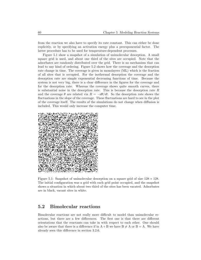
60 Chapter 5. Modeling Reaction Systems
from the reaction we also have to specify its rate constant. This can either be doneexplicitly, or by specifying an activation energy plus a preexponential factor. Thelatter procedure has to be used for temperature-dependent processes.
Figure 5.1 show a snapshot of a simulation of unimolecular desorption. A smallsquare grid is used, and about one third of the sites are occupied. Note that theadsorbates are randomly distributed over the grid. There is no mechanism that canlead to any kind of ordering. Figure 5.2 shows how the coverage and the desorptionrate change in time. The coverage is given in monolayers (ML) which is the fractionof all sites that is occupied. For the isothermal desorption the coverage and thedesorption rate are simple exponential decreasing functions of time. Because thesystem is not very big, there is a clear difference in the figures for the coverage andfor the desorption rate. Whereas the coverage shows quite smooth curves, thereis substantial noise in the desorption rate. This is because the desorption rate Rand the coverage θ are related via R = −dθ/dt. So the desorption rate shows thefluctuations in the slope of the coverage. These fluctuations are hard to see in the plotof the coverage itself. The results of the simulations do not change when diffusion isincluded. This would only increase the computer time.
Figure 5.1: Snapshot of unimolecular desorption on a square grid of size 128 × 128.The initial configuration was a grid with each grid point occupied, and the snapshotshows a situation in which about two third of the sites has been vacated. Adsorbatesare in black, vacant sites in white.
5.2 Bimolecular reactions
Bimolecular reactions are not really more difficult to model than unimolecular re-actions, but there are a few differences. The first one is that there are differentorientations that the reactants can take in with respect to each other. One shouldalso be aware that there is a difference if in A+B we have B 6= A or B = A. We havealready seen this difference in section 3.2.6.
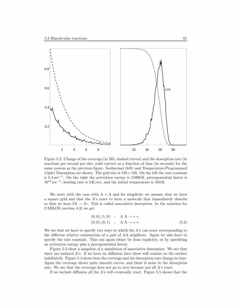
5.2 Bimolecular reactions 61
0.8
0.6
0.4
0.2
2 4 6 8 20 40 60 80
x16
Figure 5.2: Change of the coverage (in ML; dashed curves) and the desorption rate (inreactions per second per site; solid curves) as a function of time (in seconds) for thesame system as the previous figure. Isothermal (left) and Temperature-Programmed(right) Desorption are shown. The grid size is 128×128. On the left the rate constantis 0.4 sec−1. On the right the activation energy is 15000 K, preexponential factor is1013 sec−1, heating rate is 2 K/sec, and the initial temperature is 350 K.
We start with the case with A + A and for simplicity we assume that we havea square grid and that the A’s react to form a molecule that immediately desorbsso that we have 2A → 2∗. This is called associative desorption. In the notation forCARLOS (section 4.3) we get
(0, 0), (1, 0) : A A → ∗ ∗,(0, 0), (0, 1) : A A → ∗ ∗. (5.2)
We see that we have to specify two ways in which the A’s can react corresponding tothe different relative orientations of a pair of AA neighbors. Again we also have tospecify the rate constant. This can again either be done explicitly, or by specifyingan activation energy plus a preexponential factor.
Figure 5.3 show a snapshot of a simulation of associative desorption. We see thatthere are isolated A’s. If we have no diffusion then these will remain on the surfaceindefinitely. Figure 5.4 shows how the coverage and the desorption rate change in time.Again the coverage shows quite smooth curves, and there is noise in the desorptionrate. We see that the coverage does not go to zero because not all A’s react.
If we include diffusion all the A’s will eventually react. Figure 5.5 shows that the
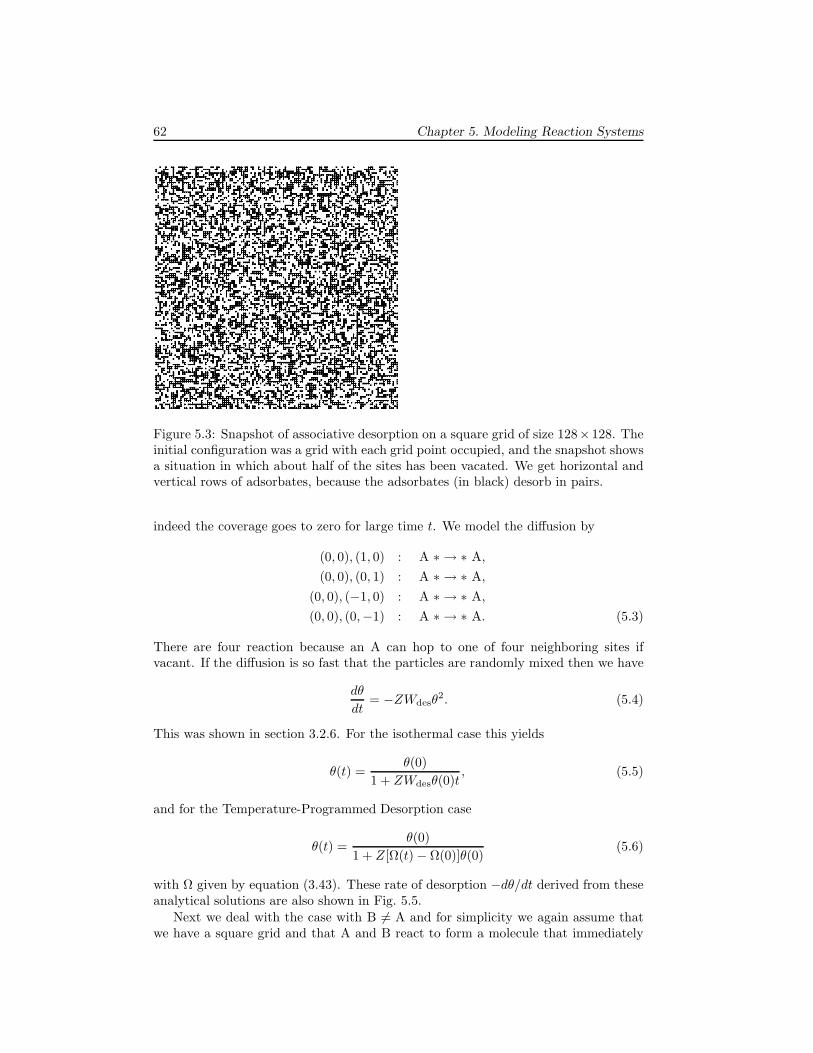
62 Chapter 5. Modeling Reaction Systems
Figure 5.3: Snapshot of associative desorption on a square grid of size 128×128. Theinitial configuration was a grid with each grid point occupied, and the snapshot showsa situation in which about half of the sites has been vacated. We get horizontal andvertical rows of adsorbates, because the adsorbates (in black) desorb in pairs.
indeed the coverage goes to zero for large time t. We model the diffusion by
(0, 0), (1, 0) : A ∗ → ∗ A,
(0, 0), (0, 1) : A ∗ → ∗ A,
(0, 0), (−1, 0) : A ∗ → ∗ A,
(0, 0), (0,−1) : A ∗ → ∗ A. (5.3)
There are four reaction because an A can hop to one of four neighboring sites ifvacant. If the diffusion is so fast that the particles are randomly mixed then we have
dθ
dt= −ZWdesθ
2. (5.4)
This was shown in section 3.2.6. For the isothermal case this yields
θ(t) =θ(0)
1 + ZWdesθ(0)t, (5.5)
and for the Temperature-Programmed Desorption case
θ(t) =θ(0)
1 + Z[Ω(t) − Ω(0)]θ(0)(5.6)
with Ω given by equation (3.43). These rate of desorption −dθ/dt derived from theseanalytical solutions are also shown in Fig. 5.5.
Next we deal with the case with B 6= A and for simplicity we again assume thatwe have a square grid and that A and B react to form a molecule that immediately
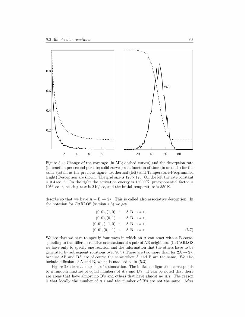
5.2 Bimolecular reactions 63
0.8
0.6
0.4
0.2
2 4 6 8 20 40 60 80
x40
Figure 5.4: Change of the coverage (in ML; dashed curves) and the desorption rate(in reaction per second per site; solid curves) as a function of time (in seconds) for thesame system as the previous figure. Isothermal (left) and Temperature-Programmed(right) Desorption are shown. The grid size is 128×128. On the left the rate constantis 0.4 sec−1. On the right the activation energy is 15000 K, preexponential factor is1013 sec−1, heating rate is 2 K/sec, and the initial temperature is 350 K.
desorbs so that we have A + B → 2∗. This is called also associative desorption. Inthe notation for CARLOS (section 4.3) we get
(0, 0), (1, 0) : A B → ∗ ∗,(0, 0), (0, 1) : A B → ∗ ∗,
(0, 0), (−1, 0) : A B → ∗ ∗,(0, 0), (0,−1) : A B → ∗ ∗. (5.7)
We see that we have to specify four ways in which an A can react with a B corre-sponding to the different relative orientations of a pair of AB neighbors. (In CARLOSwe have only to specify one reaction and the information that the others have to begenerated by subsequent rotations over 90.) These are two more than for 2A → 2∗,because AB and BA are of course the same when A and B are the same. We alsoinclude diffusion of A and B, which is modeled as in (5.3).
Figure 5.6 show a snapshot of a simulation. The initial configuration correspondsto a random mixture of equal numbers of A’s and B’s. It can be noted that thereare areas that have almost no B’s and others that have almost no A’s. The reasonis that locally the number of A’s and the number of B’s are not the same. After
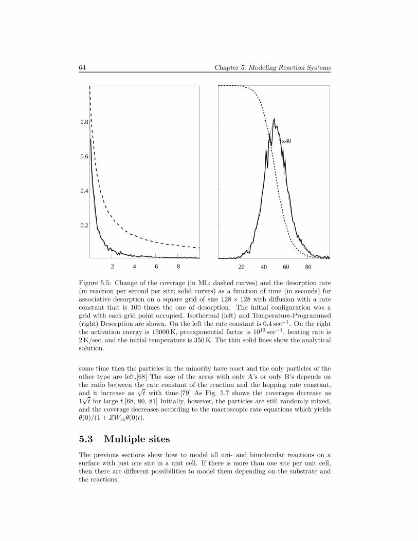
64 Chapter 5. Modeling Reaction Systems
8
0.8
0.6
0.4
0.2
2 4 6 20 40 60 80
x40
Figure 5.5: Change of the coverage (in ML; dashed curves) and the desorption rate(in reaction per second per site; solid curves) as a function of time (in seconds) forassociative desorption on a square grid of size 128 × 128 with diffusion with a rateconstant that is 100 times the one of desorption. The initial configuration was agrid with each grid point occupied. Isothermal (left) and Temperature-Programmed(right) Desorption are shown. On the left the rate constant is 0.4 sec−1. On the rightthe activation energy is 15000 K, preexponential factor is 1013 sec−1, heating rate is2 K/sec, and the initial temperature is 350 K. The thin solid lines show the analyticalsolution.
some time then the particles in the minority have react and the only particles of theother type are left.[68] The size of the areas with only A’s or only B’s depends onthe ratio between the rate constant of the reaction and the hopping rate constant,and it increase as
√t with time.[79] As Fig. 5.7 shows the coverages decrease as
1√
t for large t.[68, 80, 81] Initially, however, the particles are still randomly mixed,and the coverage decreases according to the macroscopic rate equations which yieldsθ(0)/(1 + ZWrxθ(0)t).
5.3 Multiple sites
The previous sections show how to model all uni- and bimolecular reactions on asurface with just one site in a unit cell. If there is more than one site per unit cell,then there are different possibilities to model them depending on the substrate andthe reactions.
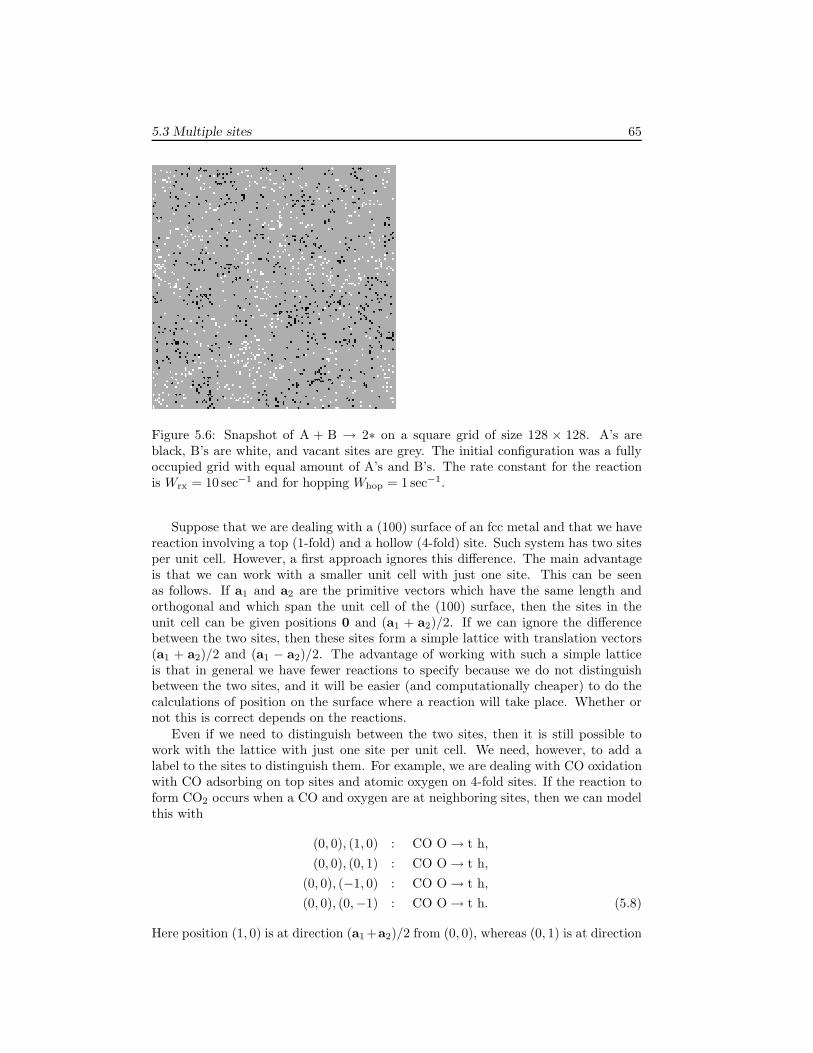
5.3 Multiple sites 65
Figure 5.6: Snapshot of A + B → 2∗ on a square grid of size 128 × 128. A’s areblack, B’s are white, and vacant sites are grey. The initial configuration was a fullyoccupied grid with equal amount of A’s and B’s. The rate constant for the reactionis Wrx = 10 sec−1 and for hopping Whop = 1 sec−1.
Suppose that we are dealing with a (100) surface of an fcc metal and that we havereaction involving a top (1-fold) and a hollow (4-fold) site. Such system has two sitesper unit cell. However, a first approach ignores this difference. The main advantageis that we can work with a smaller unit cell with just one site. This can be seenas follows. If a1 and a2 are the primitive vectors which have the same length andorthogonal and which span the unit cell of the (100) surface, then the sites in theunit cell can be given positions 0 and (a1 + a2)/2. If we can ignore the differencebetween the two sites, then these sites form a simple lattice with translation vectors(a1 + a2)/2 and (a1 − a2)/2. The advantage of working with such a simple latticeis that in general we have fewer reactions to specify because we do not distinguishbetween the two sites, and it will be easier (and computationally cheaper) to do thecalculations of position on the surface where a reaction will take place. Whether ornot this is correct depends on the reactions.
Even if we need to distinguish between the two sites, then it is still possible towork with the lattice with just one site per unit cell. We need, however, to add alabel to the sites to distinguish them. For example, we are dealing with CO oxidationwith CO adsorbing on top sites and atomic oxygen on 4-fold sites. If the reaction toform CO2 occurs when a CO and oxygen are at neighboring sites, then we can modelthis with
(0, 0), (1, 0) : CO O → t h,
(0, 0), (0, 1) : CO O → t h,
(0, 0), (−1, 0) : CO O → t h,
(0, 0), (0,−1) : CO O → t h. (5.8)
Here position (1, 0) is at direction (a1 +a2)/2 from (0, 0), whereas (0, 1) is at direction
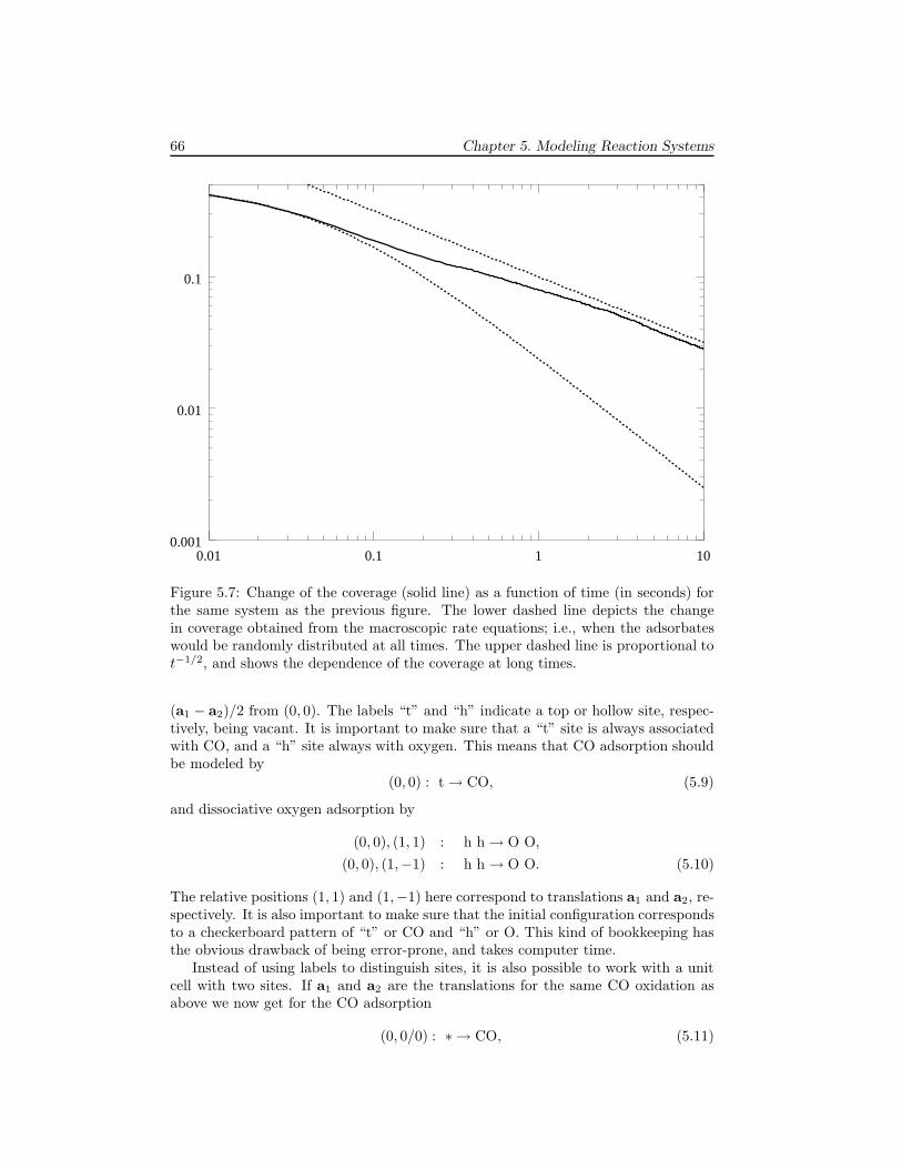
66 Chapter 5. Modeling Reaction Systems
0.001
0.01
0.01 0.1 1 10
0.1
Figure 5.7: Change of the coverage (solid line) as a function of time (in seconds) forthe same system as the previous figure. The lower dashed line depicts the changein coverage obtained from the macroscopic rate equations; i.e., when the adsorbateswould be randomly distributed at all times. The upper dashed line is proportional tot−1/2, and shows the dependence of the coverage at long times.
(a1 − a2)/2 from (0, 0). The labels “t” and “h” indicate a top or hollow site, respec-tively, being vacant. It is important to make sure that a “t” site is always associatedwith CO, and a “h” site always with oxygen. This means that CO adsorption shouldbe modeled by
(0, 0) : t → CO, (5.9)
and dissociative oxygen adsorption by
(0, 0), (1, 1) : h h → O O,
(0, 0), (1,−1) : h h → O O. (5.10)
The relative positions (1, 1) and (1,−1) here correspond to translations a1 and a2, re-spectively. It is also important to make sure that the initial configuration correspondsto a checkerboard pattern of “t” or CO and “h” or O. This kind of bookkeeping hasthe obvious drawback of being error-prone, and takes computer time.
Instead of using labels to distinguish sites, it is also possible to work with a unitcell with two sites. If a1 and a2 are the translations for the same CO oxidation asabove we now get for the CO adsorption
(0, 0/0) : ∗ → CO, (5.11)
5.4 Systems without translational symmetry 67
with the third “O” in (0, 0/0) referring to the top site in the unit cell. The dissociativeadsorption of oxygen becomes
(0, 0/1), (1, 0/1) : ∗ ∗ → O O,
(0, 0/1), (0, 1/1) : ∗ ∗ → O O. (5.12)
The “1” in (0, 0/1) indicates the hollow site. Note that we can now use the same labelfor any vacant site. The oxidation reaction becomes
(0, 0/0), (0, 0/1) : CO O → ∗ ∗,(0, 0/0), (−1, 0/1) : CO O → ∗ ∗,(0, 0/0), (0,−1/1) : CO O → ∗ ∗,
(0, 0/0), (−1,−1/1) : CO O → ∗ ∗. (5.13)
Whether it is better to use labels to distinguish the sites or to work with a unitcell with two sites depends on the reactions and the substrate. Also coding may playa role. Calculations of the positions of where reactions can take place can often bedone more efficient when the grid sizes are powers of two. If we use labels, then thismight not be possible. For example, suppose we have a (111) surface of an fcc metaland we are dealing with top and the two hollow sites. These form again a simplelattice, but if we use this simple lattice then we have to work with system sizes thatare multiples of three.
5.4 Systems without translational symmetry
The simulations always assume that the sites form a lattice. The previous sectionon multiple sites has shown that by adding labels specifying extra properties to asite we can modify the lattice. We can use this even to model a system that has notranslational symmetry while still using a lattice.
Suppose we want to model a stepped surface. We can model such a surface witha large unit cell and multiple sites. This may not be a good idea, however. Wewill be dealing with many sites per unit cell, and we will have to specify for eachits reactions. This will generally lead to a long list of reactions, even if the differentsites on the terraces have the same properties, and only the sites at the steps behavedifferently. In such a case it is better to use a label to distinguish to sites at the step.For example, if we are dealing with simple desorption of an adsorbate A then we canmodel desorption from a terrace site as
(0, 0) : A → ∗. (5.14)
Desorption from a site at the step becomes
(0, 0) : As → ∗s. (5.15)
We add an “s” to distinguish the adsorbate on a step site and a vacant step site.Note that there is a difference with the example of CO oxidation on a (100) surfaceof the section on multiple sites. There the label “CO” already implied one type ofsite and “O” another. Here the same adsorbate can be found on both types of sites.We also need to specify different rate constants for the desorption for both types of
68 Chapter 5. Modeling Reaction Systems
sites, because otherwise distinguishing them would not be meaningful. The preciseposition of the steps has to be specified in the initial configuration.
For a unimolecular reaction we need to specify just two reactions. If we havea bimolecular reaction we need to specify reactions for all possible combinations ofoccupations of step and terrace sites. So if we have a reaction A + B → 2∗, then wewill have A B → ∗ ∗, As B → ∗s ∗, A Bs → ∗ ∗s, and As Bs → ∗s ∗s. Diffusioncan also be regarded as a bimolecular reaction, and we need to specify A ∗ → ∗ A,As ∗ → ∗s A, A ∗s → ∗ As, and As ∗s → ∗s As for the diffusion of A. Needless to
say that all these possibilities will have in general different rate constants.The procedure above will be unavoidable if we have point defects that are not
regularly distributed over the surface. The specification of the initial configurationdetermines where the defects are. It is of course possible to have more than one typeof defect.
On a surface with defects most sites usually are normal sites and only a minorityis a defect site. The procedure above can also be used when that is not the case.This means that we can use it to model a surface of a bimetallic catalyst. Only theinterpretation of the label changes; it will not indicate a normal or step site, but asite on one or the other metal. If there are reactions that are not affected by thetype of metal on which it occurs, another model may be more efficient. Suppose thatwe have one site per unit cell disregarding the difference between the metals and alladsorbates occupy top sites. We then specify an imaginary second site. The first sitegets the adsorbate and the second has to label specifying the metal. The second sitedoesn’t actually exist. There is only one site, but we split the information on this sitein two. With adsorbate A and metal M1 and M2 we have
(0, 0/0), (0, 0/1) : A M1 → ∗ M1 (5.16)
and(0, 0/0), (0, 0/1) : A M2 → ∗ M2 (5.17)
for desorption. In the previous models we combined the information on the adsorbateand the site in one label. Here we keep that information apart. This is advantageous ifthere is a reaction that does not depend on the metal. So if diffusion of the adsorbateis equally fast on both metals, we can model this with
(0, 0/0), (1, 0/0) : A ∗ → ∗ A (5.18)
and similar expressions for hops to other neighboring sites. We see that there isno information on the metal. This would not be possible if the information on theadsorbate and the information on the metal would have been combined.
So far the occupation of the sites have been allowed to change through reactions,but the properties of the sites themselves have been fixed. This need not always bethe case. The surface composition of a bimetallic catalyst may change, or we might bedealing with a reconstructing surface. For a reconstructing surface we can introduce alabel that specifies to which phase of the substrate a site belongs. A change of surfacecomposition of a bimetallic catalyst or a reconstruction can be modeled with reactionsthat specify the changes in the substrate. For example, there have been many studiesof CO oxidation on reconstructing platinum surfaces. In one of the simplest modelsof this process there are reaction for the growth of the phases.[13, 14, 82] One phase,called the α phase, growths if there are no adsorbates. This can be modeled by
(0, 0/1), (0, 0/0), (1, 0/1), (1, 0/0) : α ∗ β ∗ → α ∗ α ∗. (5.19)
5.5 Infinitely fast reactions 69
The β phase growths in an area with sites occupied by CO.
(0, 0/1), (0, 0/0), (1, 0/1), (1, 0/0) : β CO α CO → β CO β CO. (5.20)
It should be realized that there are restrictions in what one can do with a changingsubstrate in DMC simulations. One does need to be able to put everything on a grid.Reconstructions that lead, for example, to surface structure with a different densitycan only be modeled if this change is ignored. Also changes of the local point-groupsymmetry may not be possible to model.
5.5 Infinitely fast reactions
Sometimes a reaction is so much faster than the other reactions in a system that oneregard may as an infinitely fast reaction. This has the advantage that one doesn’tneed to compute the time when that reaction takes place. One simply checks ifthe sites involved are occupied by the correct reactants and then replaces them bythe products without changing the time. More difficult are situations where morethan one infinitely fast reaction are possible but not all of them can actually takeplace. Sometimes one can choose a reaction at random, sometimes one needs to givedifferent infinite reactions different priorities. There are also situations when it isbetter to incorporate a fast reaction in another reaction, and there are situationswhere one doesn’t actually have infinitely fast reactions, but they can be useful in themodeling. CARLOS (see section 4.3) calls these infinitely fast reactions immediatereactions.
Suppose we have a system with three reactions; simple adsorption of A’s, simpleadsorption of B’s, and when an A occupies a site next to a B they react and theproduct desorbs. We will look at the case where the reaction A+B and the desorptionis infinitely fast; i.e., we have with infinitely large rate constant A + B → 2∗ as far asthe occupation of the sites is concerned. If the rate constant for adsorption of A (B)is larger than the one for adsorption of B (A), then after some time the surface willbecome completely covered by A’s (B’s). We will therefore only look at the situationin which A and B have the same rate constant for adsorption. In this system itcan occur that there is a vacant site with two or more neighboring sites that areoccupied by B’s. If an A adsorbs onto the vacant site, then it can react with eitherof the neighboring B’s. It seems obvious to pick the B with which the A will reactat random. Similarly, if a B adsorbs at a site where it gets two or more A neighbors,then it will react with one of them which should be picked at random.
Actually we have implicitly assumed in the previous paragraph that all neighborsare equivalent. This is the case for example on a square grid that represents a (100)surface of an fcc metal, or a hexagonal grid that represents a (111) surface of an fccmetal. This is not the case for a rectangular grid that represents a (110) surface ofan fcc metal. There is a different rate constant for a reaction with a neighboring inone direction than for the direction perpendicular to it. It is possible in this situationto have different priorities for the infinitely fast reactions. Suppose an A has a Bneighbor in direction 1 and a B neighbor in direction 2. It will react with bothof them infinitely fast, but it prefers to react with the one in direction 1. In sucha situation one should give the reaction with the neighbor in direction 1 a higherpriority. So first check if there are AB pairs oriented in direction 1. If this is the case
70 Chapter 5. Modeling Reaction Systems
then have them react. If there is more than one of such a pair then if necessary tochoose at random among the different pairs. After there are no more of such pairs,then check for AB pairs oriented in direction 2, and react them.
One can also remove the infinitely fast reaction altogether. Straightforward mod-eling as above yields
(0, 0) : ∗ → A (5.21)
for the adsorption, and(0, 0), (1, 0) : A B → ∗ ∗ (5.22)
plus symmetry-related expressions for the infinitely fast reaction. We can now com-bine these two reactions. For example an adsorption on a site with vacant neighboringsites can be modeled as
(0, 1),(−1, 0), (0, 0), (1, 0),
(0,−1):
∗∗ ∗ ∗
∗→
∗∗ A ∗
∗. (5.23)
For simplicity we have assumed that we have a square grid. The rate constant for thisreaction equals the rate constant for adsorption. More interesting is the adsorptionon a site with one B neighbor. We then have
(0, 1),(−1, 0), (0, 0), (1, 0),
(0,−1):
∗∗ ∗ B
∗→
∗∗ ∗ ∗
∗. (5.24)
The adsorption takes place at (0, 0), but there is an immediate reaction with the Bso that the sites at (0, 0) and (1, 0) become vacant again. On a square grid there arethree other symmetry-related reactions. The rate constant for each of them is againthe rate constant for adsorption. If there are two B neighbors we get
(0, 1),(−1, 0), (0, 0), (1, 0),
(0,−1):
B∗ ∗ B
∗→
B∗ ∗ ∗
∗(5.25)
and symmetry-related reactions or
(0, 1),(−1, 0), (0, 0), (1, 0),
(0,−1):
∗B ∗ B
∗→
∗B ∗ ∗
∗(5.26)
and symmetry-related reactions. In both reactions there are two possibilities for A toreact. This affects the rate constant. Suppose we have at time t the situation
∗B ∗ B
∗(5.27)
and an A adsorbs in the middle. This adsorption takes on average a time W−1ads, where
Wads is the rate constant for adsorption. So after adsorption we are on average attime t + W−1
ads and have the situation
∗B A B
∗. (5.28)
5.5 Infinitely fast reactions 71
Next the A reacts with one of the B’s to give
∗∗ ∗ B
∗, or
∗B ∗ ∗
∗(5.29)
with equal probability, and we are still at time t + W−1ads. If use the second method
of modeling the reactions, then we go directly from the initial to one of the finalsituations. If the rate constant for each of the reactions is W2B, then on average thereaction takes place at time t + (2W2B)−1. We get a factor 1/2, because in the initialsituations there are two reactions possible. The total rate constant for that situationis the sum of the rate constants of all possible reactions; i.e., 2W2B. To get the sameresult as before we therefore must have W2B = Wads/2. In general, if we have N Bneighbors in the initial situation then the direct reactions should have a rate constantthat is equal to the rate constant for adsorption divided by N .
Whether removing the infinitely fast reactions is efficient will depend on the sys-tem, but it is more common to introduce such reactions rather than to remove them.Introducing infinitely fast reactions need not be restricted to reactions that actual oc-cur. In fact, the reactions we introduce are generally ones that exist only in the modeland not in reality. Suppose that we have adsorption of a somewhat bulky adsorbateA. The adsorbate occupies not only a particular site, but also makes it impossiblefor other adsorbates to occupy neighboring sites. On a square grid we might try tomodel this as follows.
(0, 1),(−1, 0), (0, 0), (1, 0),
(0,−1):
∗∗ ∗ ∗
∗→
AtAl A Ar
Ab(5.30)
where the labels on the right stand for the adsorbate, and blocked sites above, left,right, and below, respectively. (Having all five sites getting a label A is not a good idea,because after more adsorbates have adsorbed you won’t be able to tell which A standsfor an adsorbate and which stands for a blocked site.) The drawback of this model isthat effectively more than these four neighboring sites are blocked. For example, itis not possible for another A to adsorb on site (1, 1) because such adsorption aboveneeds ∗ on (1, 0) and (0, 1) whereas there are Ar and Aa, respectively.
This problem can be solved with infinitely fast reactions. The adsorption we modelsimply with
(0, 0) : ∗ → A. (5.31)
This reaction has a finite rate constant. The blocking of the neighboring sites ismodeled with
(0, 0), (1, 0) : A ∗ → A blocked. (5.32)
This reaction, and the symmetry-related ones, are infinitely fast. In this way anotherA can adsorb on (1, 1). This seems quite straightforward, but things become a bitmore tricky when the adsorbate can also diffuse and desorb, We look at desorption,Just
(0, 0) : A → ∗ (5.33)
does not work, because this leaves “blocked” labels for sites that are not blocked anylonger,
(0, 0), (1, 0) : A blocked → ∗ ∗ (5.34)
72 Chapter 5. Modeling Reaction Systems
doesn’t work either, because this reaction can occur only once for each adsorbate,This means only one label “blocked” is changed back to ∗, but the adsorbate mayhave been blocking more than one site, What does work is first
(0, 0) : A → vacated, (5.35)
The label “vacated” indicates that an adsorbate has just desorbed from the site, It isused to remove the “blocked” labels by
(0, 0), (1, 0) : vacated blocked → vacated ∗, (5.36)
This should be an infinitely fast reaction, Note that the label “vacated” stays so thatit can remove all “blocked” labels, To get rid of the “vacated” label we finally haveanother infinitely fast reaction
(0, 0) : vacated → ∗, (5.37)
It is clear that this reaction should only occur after all “blocked” labels have beenremoved, so it should have a lower priority than the previous reaction, The last thingthat we now need to do is to give the original blocking reaction (5.32) an even lowerpriority, If we would not do that we could get the following infinite loop
∗ ∗ ∗ ∗ → ∗ A ∗ ∗→ blocked A ∗ ∗→ blocked A blocked ∗→ blocked A blocked A→ blocked vacated blocked A→ blocked vacated ∗ A→ blocked vacated blocked A→ blocked vacated ∗ A→ . . .
(5.38)
(We have looked only at the sites along one line for convenience,) With the blockingreaction having the lowest priority sites only become blocked again after the “vacated”label has been removed,
5.6 Diffusion
Diffusion is often mentioned when shortcomings of DMC are discussed, This is notquite appropriate, It is even less appropriate to say that DMC has problems whenthere are reactions with very different rate constants, This is indeed a problem whena fix step size is used, because the step size should be small enough so that the fastestreactions is simulated correctly, For the slower reactions a small step size is, however,inefficient, There is no problem with variable step sizes, Diffusion is indeed a problem,because it is often much faster than the other processes, DMC will happily simulatethis fast diffusion, but most computer time is spent on diffusion and only a very smallfraction on the other reaction, which are often the ones one really interesting in,This is not really a shortcoming of DMC, however, but reflects an intrinsic propertyof the system one is studying, Any method that simulates all processes that takeplace will have to spent most time on the diffusion simply because most events are
5.6 Diffusion 73
adsorbates moving from site to site, A similar situation arises when one has a veryfast adsorption-desorption equilibrium with most events adsorption and desorptionprocesses, Nevertheless, there are some ways to reduce the fraction of computer timethat one has to spend on diffusion,
To model diffusion one needs to have a reaction like
(0, 0), (1, 0) : A ∗ → ∗ A, (5.39)
The problem is in the rate constant and in a possible use of other reactions as well,In the simplest case one simply gives the reaction above a rate constant so that oneobtains the correct diffusion constant (see section 3.2.5), If the diffusion is not too fast(i,e,, a substantial part of the simulation is spent on other reactions), then this is allone needs to do, If the diffusion is too fast, then there are a few other options, Veryoften diffusion is so fast that it equilibrates the adlayer before another process/reactionhas taken place, In such a situation the precise rate of diffusion is not important, Aslong as this equilibration occurs, then the simulation yields correct results, This oftenmeans that it is possible to make diffusion much slower than in reality, One has tothink here about a reduction of orders of magnitude, The precise value also dependson the system size, The displacement of a particle through diffusion increase with thesquare of time, If the system is small, then it will rapidly have moved through thewhole system, If the system is large, then this will take longer, This means that forsmall systems the diffusion rate can be reduced more than for large systems,
In some algorithmic approaches of DMC fast diffusion has been simulated as fol-lows, After a particle has adsorbed it starts to diffuse over the surface, This diffusionconsists of random hops from one site to another, These hops continue until the par-ticle encounters another particle with which it can react, It then stops hopping andreacts with the other particle,[83, 84] This method was used to model CO oxidation,CO is the rapidly diffusing particle, and atomic oxygen is fixed at an adsorption site,and is the particle with which CO reacts, Diffusion was regarded as being faster thanany of the other processes, but, as the CO react with the very first oxygen that itencounters, it seems that the formation of CO2 is really even faster, If we work withinfinitely fast reaction then we have
(0, 0), (1, 0) : CO ∗ → ∗ CO (5.40)
for the diffusion, This reaction has a low priority, The formation of CO2 is representedby
(0, 0), (1, 0) : CO O → ∗ ∗ (5.41)
with a high priority,If we really want to have a diffusion faster than the oxidation, then things become
more complicated, For the diffusion we now have the infinitely fast reaction
(0, 0), (1, 0) : CO ∗ → CO CO, (5.42)
The label “CO” does not mean that there is a CO at that site, but that CO will visitthe site during its diffusion over the surface, This reaction has a high priority, say 2,The reaction is modeled via
(0, 0), (1, 0) : CO O → r r, (5.43)
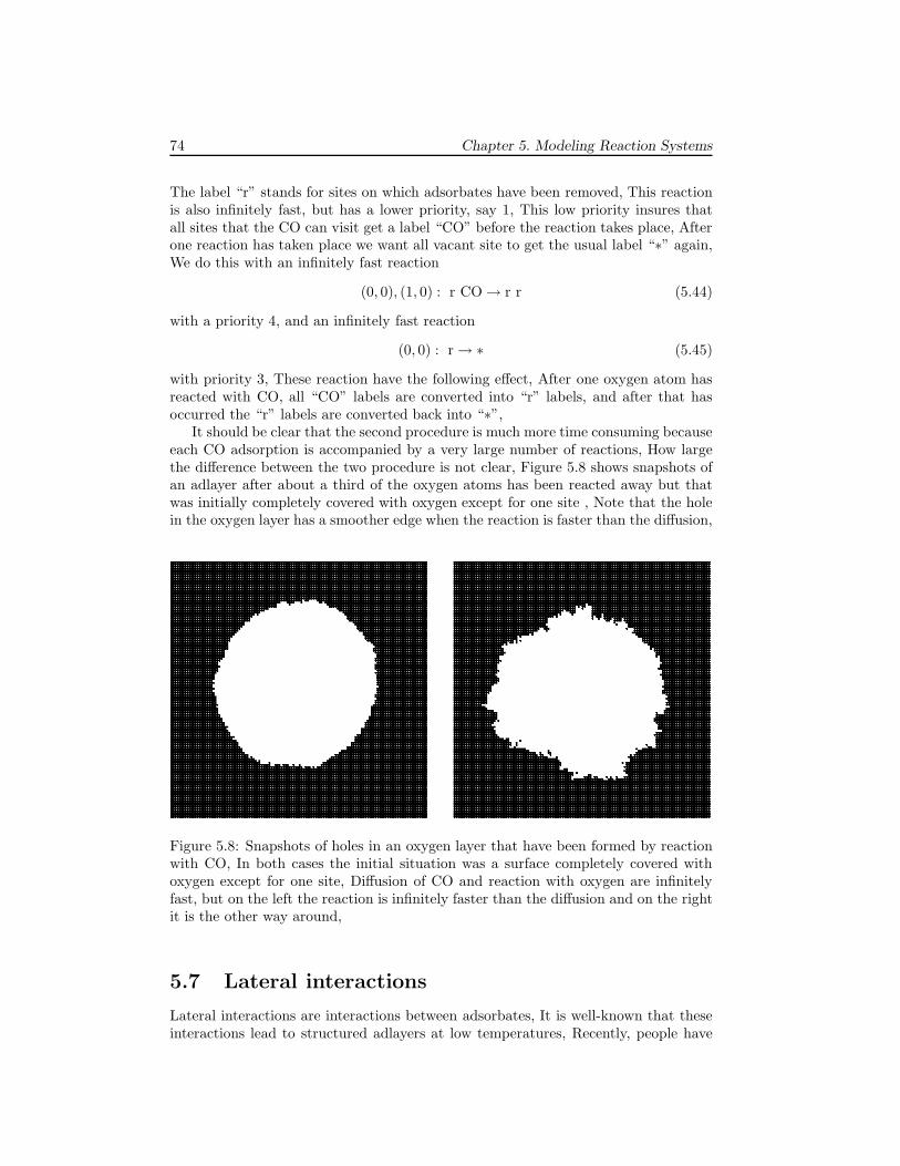
74 Chapter 5. Modeling Reaction Systems
The label “r” stands for sites on which adsorbates have been removed, This reactionis also infinitely fast, but has a lower priority, say 1, This low priority insures thatall sites that the CO can visit get a label “CO” before the reaction takes place, Afterone reaction has taken place we want all vacant site to get the usual label “∗” again,We do this with an infinitely fast reaction
(0, 0), (1, 0) : r CO → r r (5.44)
with a priority 4, and an infinitely fast reaction
(0, 0) : r → ∗ (5.45)
with priority 3, These reaction have the following effect, After one oxygen atom hasreacted with CO, all “CO” labels are converted into “r” labels, and after that hasoccurred the “r” labels are converted back into “∗”,
It should be clear that the second procedure is much more time consuming becauseeach CO adsorption is accompanied by a very large number of reactions, How largethe difference between the two procedure is not clear, Figure 5.8 shows snapshots ofan adlayer after about a third of the oxygen atoms has been reacted away but thatwas initially completely covered with oxygen except for one site , Note that the holein the oxygen layer has a smoother edge when the reaction is faster than the diffusion,
Figure 5.8: Snapshots of holes in an oxygen layer that have been formed by reactionwith CO, In both cases the initial situation was a surface completely covered withoxygen except for one site, Diffusion of CO and reaction with oxygen are infinitelyfast, but on the left the reaction is infinitely faster than the diffusion and on the rightit is the other way around,
5.7 Lateral interactions
Lateral interactions are interactions between adsorbates, It is well-known that theseinteractions lead to structured adlayers at low temperatures, Recently, people have
5.7 Lateral interactions 75
realized that the kinetics of surface reactions can be substantially affected by theseinteractions even at high temperature, Little is known about the form of these inter-actions and even less about the strength of them, In this section we present a generalbut not very efficient method, the method that is implemented in CARLOS to modelpairwise additive interactions, and a few tricks to model more complicated interac-tions with reasonable efficiency, In all cases we assume that the lateral interactionsare short range,
A general method to model lateral interaction consists of specifying the reactionand the occupation of the sites that may have adsorbates that will affect the reaction,For example, if we have a simple desorption of an adsorbate A on a square grid witha rate constant that depends on the occupation of the four neighboring sites, then wehave the reactions
(0, 1),(−1, 0), (0, 0), (1, 0),
(0,−1):
∗∗ A ∗
∗→
∗∗ ∗ ∗
∗,
(0, 1),(−1, 0), (0, 0), (1, 0),
(0,−1):
∗∗ A A
∗→
∗∗ ∗ A
∗,
(0, 1),(−1, 0), (0, 0), (1, 0),
(0,−1):
A∗ A A
∗→
A∗ ∗ A
∗, (5.46)
(0, 1),(−1, 0), (0, 0), (1, 0),
(0,−1):
∗A A A
∗→
∗A ∗ A
∗,
(0, 1),(−1, 0), (0, 0), (1, 0),
(0,−1):
AA A A
∗→
AA ∗ A
∗,
(0, 1),(−1, 0), (0, 0), (1, 0),
(0,−1):
AA A A
A→
AA ∗ A
A,
Of all symmetry-related reactions only one is shown, Each of these reactions can begiven a different rate constant (or activation energy and preexponential factor), Byspecifying all possible occupations of the neighboring sites explicitly any form of thelateral interactions can be modeled, The disadvantage should also be clear, The listof reactions can be quite long, With Z neighboring sites that may be occupied by anadsorbate that affects the reaction and A possible occupations of each of these sites(including no adsorbate) there are AZ reactions to specify,
CARLOS (see section 4.3) has the possibility to deal with lateral interactions thatchange the activation energy of a reaction in a pairwise additive manner, Let’s takethe previous example of a desorbing adsorbate A again, In CARLOS desorption canbe specified as
(0, 1),(−1, 0), (0, 0), (1, 0),
(0,−1): (5.47)
∗ A : ϕ ∗ A : ϕ A ∗ A : ϕ
∗ A : ϕ →
## ∗ #
#,
76 Chapter 5. Modeling Reaction Systems
The notation with the curly braces means that an adsorbate A at the site changes theactivation energy of the reaction by an amount ϕ, A vacant site does not change theactivation energy, The hashes (#) on the right mean that the occupation of the sitedoes not change, This way to model lateral interactions does not have the flexibilityof the more general approach, but it is definitely much easier,
Figure 5.9 shows the typical effect of lateral interactions, Interactions betweennearest neighbors are very often repulsive, On a square grid this leads the checkerboardstructure at low temperatures, (Increasing the temperature leads to via an order-disorder phase transition to a random structure,) When diffusion is slow relaxation isslow and the checkerboard does not cover the whole system, but domains are formed,If one wants to get a good idea of these domains one can change the model in thefollowing way, Instead of the reaction (5.47) one uses
(0, 1),(−1, 0), (0, 0), (1, 0),
(0,−1): (5.48)
∗2 A2 : ϕ ∗2 A2 : ϕ A1 ∗2 A2 : ϕ
∗2 A2 : ϕ →
## ∗1 #
#,
and
(0, 1),(−1, 0), (0, 0), (1, 0),
(0,−1): (5.49)
∗1 A1 : ϕ ∗1 A1 : ϕ A2 ∗1 A1 : ϕ
∗1 A1 : ϕ →
## ∗2 #
#,
In the initial condition if a site has a label ending in 1 (2) then a neighboring siteshould have a label ending in 2 (1), The reason for having two reactions representingeffectively the same reaction is that one can now give neighboring sites on output adifferent coloring, If one gives “A1” to same color as “∗2”, and “A2” the same color as“∗1”, then all sites of one domain will have the same color as can be seen in Fig, 5.9,Completely covered or vacant areas will appear as a checkerboard now,
For lateral interactions that are not pairwise additive we need not always use thegeneral method, One should always look for some simple prescription describing theenergetics, For example, suppose that the activation energy for simple desorptiondepends on the number of nearest-neighbor sites being occupied, Then this might bemodeled by the reaction
(0, 0/0), (0, 0/1) : A n → ∗ n, (5.50)
Here we have two sites per unit cell, The first is an actual site, but the second hasa label that specifies how many of the neighbors of the actual site are occupied; i,e,,the label n is number of adsorbates on neighboring sites, In CARLOS one can useinfinitely fast reactions to update the labels specifying these numbers, but one can ofcourse also implement this explicitly,
Another example would be simple desorption on a hexagonal grid with an activa-tion energy that is affected by adsorbates that are nearest neighbors and that form
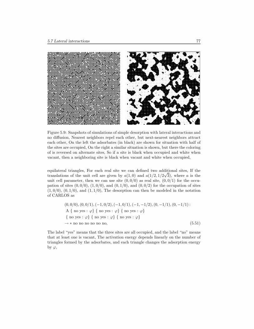
5.7 Lateral interactions 77
Figure 5.9: Snapshots of simulations of simple desorption with lateral interactions andno diffusion, Nearest neighbors repel each other, but next-nearest neighbors attracteach other, On the left the adsorbates (in black) are shown for situation with half ofthe sites are occupied, On the right a similar situation is shown, but there the coloringof is reversed on alternate sites, So if a site is black when occupied and white whenvacant, then a neighboring site is black when vacant and white when occupied,
equilateral triangles, For each real site we can defined two additional sites, If thetranslations of the unit cell are given by a(1, 0) and a(1/2, 1/2
√3), where a is the
unit cell parameter, then we can use site (0, 0/0) as real site, (0, 0/1) for the occu-pation of sites (0, 0/0), (1, 0/0), and (0, 1/0), and (0, 0/2) for the occupation of sites(1, 0/0), (0, 1/0), and (1, 1/0), The desorption can then be modeled in the notationof CARLOS as
(0, 0/0), (0, 0/1), (−1, 0/2), (−1, 0/1), (−1,−1/2), (0,−1/1), (0,−1/1) :
A no yes : ϕ no yes : ϕ no yes : ϕ no yes : ϕ no yes : ϕ no yes : ϕ→ ∗ no no no no no no, (5.51)
The label “yes” means that the three sites are all occupied, and the label “no” meansthat at least one is vacant, The activation energy depends linearly on the number oftriangles formed by the adsorbates, and each triangle changes the adsorption energyby ϕ,

78 Chapter 5. Modeling Reaction Systems
Chapter 6
Examples
This chapter is somewhat similar to chapter 5 on how to model reaction systems,However, the emphasize here is more on the information one can get from DMCsimulations; i,e,, the reason why one wants to do DMC simulations instead of usingconventional macroscopic rate equations,
6.1 The Ziff-Gulari-Barshad model
Although the work by Ziff, Gulari, and Barshad does not represent the first applicationof Monte Carlo to model surface reactions it is probably the most influential workof its type,[85] There are several reasons for that, It deals with CO oxidation whichwas and still is a very important process in catalysis and surface science, It is a verysimple model, which makes it generic, Its simplicity also made it possible to analyze indetail the relation between the microscopic reactions and the macroscopic properties,It showed the shortcomings of the macroscopic rate equations and what the origin ofthese shortcomings were, It showed that these DMC simulations could yield so-calledkinetic or non-equilibrium phase transitions, In fact, apart from the first-order phasetransition also known from macroscopic rate equations, it showed that there was acontinuous phase transition as well,
We present here the model, which we will call the ZGB-model, in its generic form,There are two adsorbates; A and B, If one wants to use the ZGB-model for COoxidation, then A stands for CO and B for atomic oxygen, There are three reactionsin the model, Adsorbate A can adsorb at single vacant sites, Adsorbate B can adsorb,but as it forms diatomic molecules in the gas phase, two neighboring vacant sitesare needed, An A will react with a B if they are nearest neighbors, This reactions isinfinitely fast, so this takes place immediately after an adsorption, We can write thereaction as
A(gas) + ∗ → A(ads)
B2(gas) + 2∗ → 2B(ads) (6.1)
A(ads) + B(ads) → AB(gas) + 2∗
where ∗ is a vacant site, “ads” stands for an adsorbed species, and “gas” for a speciesin the gas phase, The reactions involving two sites can only take place on neighboring
79
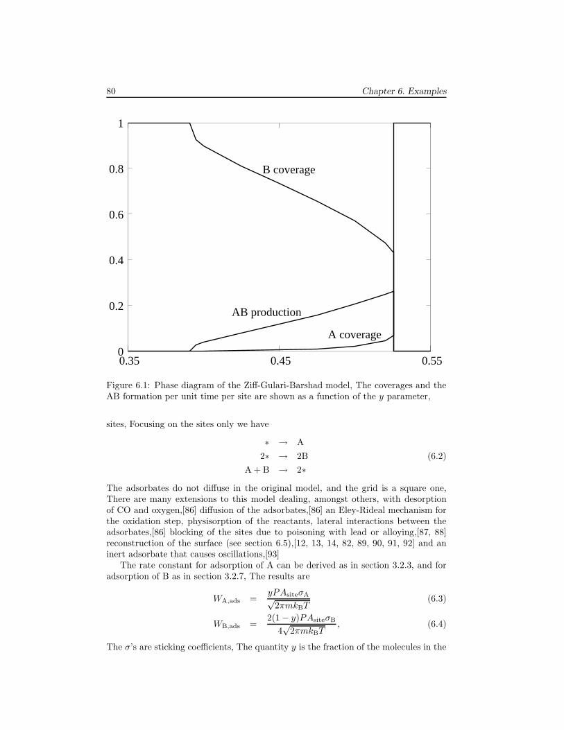
80 Chapter 6. Examples
0
0.2
0.4
0.6
0.8
1
0.35 0.45 0.55
AB production
B coverage
A coverage
Figure 6.1: Phase diagram of the Ziff-Gulari-Barshad model, The coverages and theAB formation per unit time per site are shown as a function of the y parameter,
sites, Focusing on the sites only we have
∗ → A
2∗ → 2B (6.2)
A + B → 2∗
The adsorbates do not diffuse in the original model, and the grid is a square one,There are many extensions to this model dealing, amongst others, with desorptionof CO and oxygen,[86] diffusion of the adsorbates,[86] an Eley-Rideal mechanism forthe oxidation step, physisorption of the reactants, lateral interactions between theadsorbates,[86] blocking of the sites due to poisoning with lead or alloying,[87, 88]reconstruction of the surface (see section 6.5),[12, 13, 14, 82, 89, 90, 91, 92] and aninert adsorbate that causes oscillations,[93]
The rate constant for adsorption of A can be derived as in section 3.2.3, and foradsorption of B as in section 3.2.7, The results are
WA,ads =yPAsiteσA√
2πmkBT(6.3)
WB,ads =2(1 − y)PAsiteσB
4√
2πmkBT, (6.4)
The σ’s are sticking coefficients, The quantity y is the fraction of the molecules in the
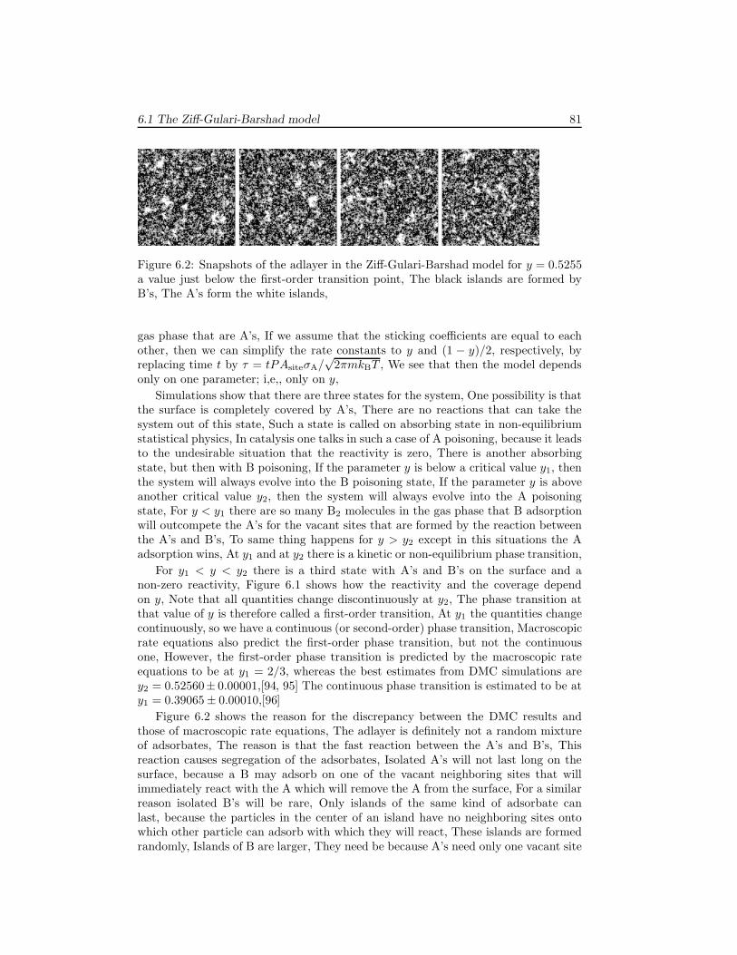
6.1 The Ziff-Gulari-Barshad model 81
Figure 6.2: Snapshots of the adlayer in the Ziff-Gulari-Barshad model for y = 0.5255a value just below the first-order transition point, The black islands are formed byB’s, The A’s form the white islands,
gas phase that are A’s, If we assume that the sticking coefficients are equal to eachother, then we can simplify the rate constants to y and (1 − y)/2, respectively, byreplacing time t by τ = tPAsiteσA/
√2πmkBT , We see that then the model depends
only on one parameter; i,e,, only on y,
Simulations show that there are three states for the system, One possibility is thatthe surface is completely covered by A’s, There are no reactions that can take thesystem out of this state, Such a state is called on absorbing state in non-equilibriumstatistical physics, In catalysis one talks in such a case of A poisoning, because it leadsto the undesirable situation that the reactivity is zero, There is another absorbingstate, but then with B poisoning, If the parameter y is below a critical value y1, thenthe system will always evolve into the B poisoning state, If the parameter y is aboveanother critical value y2, then the system will always evolve into the A poisoningstate, For y < y1 there are so many B2 molecules in the gas phase that B adsorptionwill outcompete the A’s for the vacant sites that are formed by the reaction betweenthe A’s and B’s, To same thing happens for y > y2 except in this situations the Aadsorption wins, At y1 and at y2 there is a kinetic or non-equilibrium phase transition,
For y1 < y < y2 there is a third state with A’s and B’s on the surface and anon-zero reactivity, Figure 6.1 shows how the reactivity and the coverage dependon y, Note that all quantities change discontinuously at y2, The phase transition atthat value of y is therefore called a first-order transition, At y1 the quantities changecontinuously, so we have a continuous (or second-order) phase transition, Macroscopicrate equations also predict the first-order phase transition, but not the continuousone, However, the first-order phase transition is predicted by the macroscopic rateequations to be at y1 = 2/3, whereas the best estimates from DMC simulations arey2 = 0.52560± 0.00001,[94, 95] The continuous phase transition is estimated to be aty1 = 0.39065± 0.00010,[96]
Figure 6.2 shows the reason for the discrepancy between the DMC results andthose of macroscopic rate equations, The adlayer is definitely not a random mixtureof adsorbates, The reason is that the fast reaction between the A’s and B’s, Thisreaction causes segregation of the adsorbates, Isolated A’s will not last long on thesurface, because a B may adsorb on one of the vacant neighboring sites that willimmediately react with the A which will remove the A from the surface, For a similarreason isolated B’s will be rare, Only islands of the same kind of adsorbate canlast, because the particles in the center of an island have no neighboring sites ontowhich other particle can adsorb with which they will react, These islands are formedrandomly, Islands of B are larger, They need be because A’s need only one vacant site
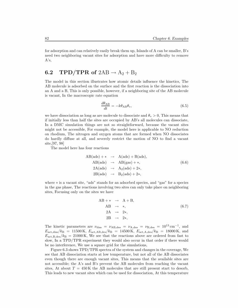
82 Chapter 6. Examples
for adsorption and can relatively easily break them up, Islands of A can be smaller, B’sneed two neighboring vacant sites for adsorption and have more difficulty to removeA’s,
6.2 TPD/TPR of 2AB → A2 + B2
The model in this section illustrates how atomic details influence the kinetics, TheAB molecule is adsorbed on the surface and the first reaction is the dissociation intoan A and a B, This is only possible, however, if a neighboring site of the AB moleculeis vacant, In the macroscopic rate equation
dθAB
dt= −kθABθ∗, (6.5)
we have dissociation as long as are molecule to dissociate and θ∗ > 0, This means thatif initially less than half the sites are occupied by AB’s all molecules can dissociate,In a DMC simulation things are not so straightforward, because the vacant sitesmight not be accessible, For example, the model here is applicable to NO reductionon rhodium, The nitrogen and oxygen atoms that are formed when NO dissociatesdo hardly diffuse at all, and severely restrict the motion of NO to find a vacantsite,[97, 98]
The model here has four reactions
AB(ads) + ∗ → A(ads) + B(ads),
AB(ads) → AB(gas) + ∗, (6.6)
2A(ads) → A2(ads) + 2∗,2B(ads) → B2(ads) + 2∗,
where ∗ is a vacant site, “ads” stands for an adsorbed species, and “gas” for a speciesin the gas phase, The reactions involving two sites can only take place on neighboringsites, Focusing only on the sites we have
AB + ∗ → A + B,
AB → ∗, (6.7)
2A → 2∗,2B → 2∗,
The kinetic parameters are νdiss = νAB,des = νA,des = νB,des = 1013 cm−1, andEact,diss/kB = 11500 K, Eact,AB,des/kB = 14500 K, Eact,A,des/kB = 18000 K, andEact,B,des/kB = 21000 K, We see that the reactions above are ordered from fast toslow, In a TPD/TPR experiment they would also occur in that order if there wouldbe no interference, We use a square grid for the simulations,
Figure 6.3 shows TPD/TPR spectra of the system and changes in the coverage, Wesee that AB dissociation starts at low temperature, but not all of the AB dissociateseven though there are enough vacant sites, This means that the available sites arenot accessible; the A’s and B’s prevent the AB molecules from reaching the vacantsites, At about T = 450 K the AB molecules that are still present start to desorb,This leads to new vacant sites which can be used for dissociation, At this temperature
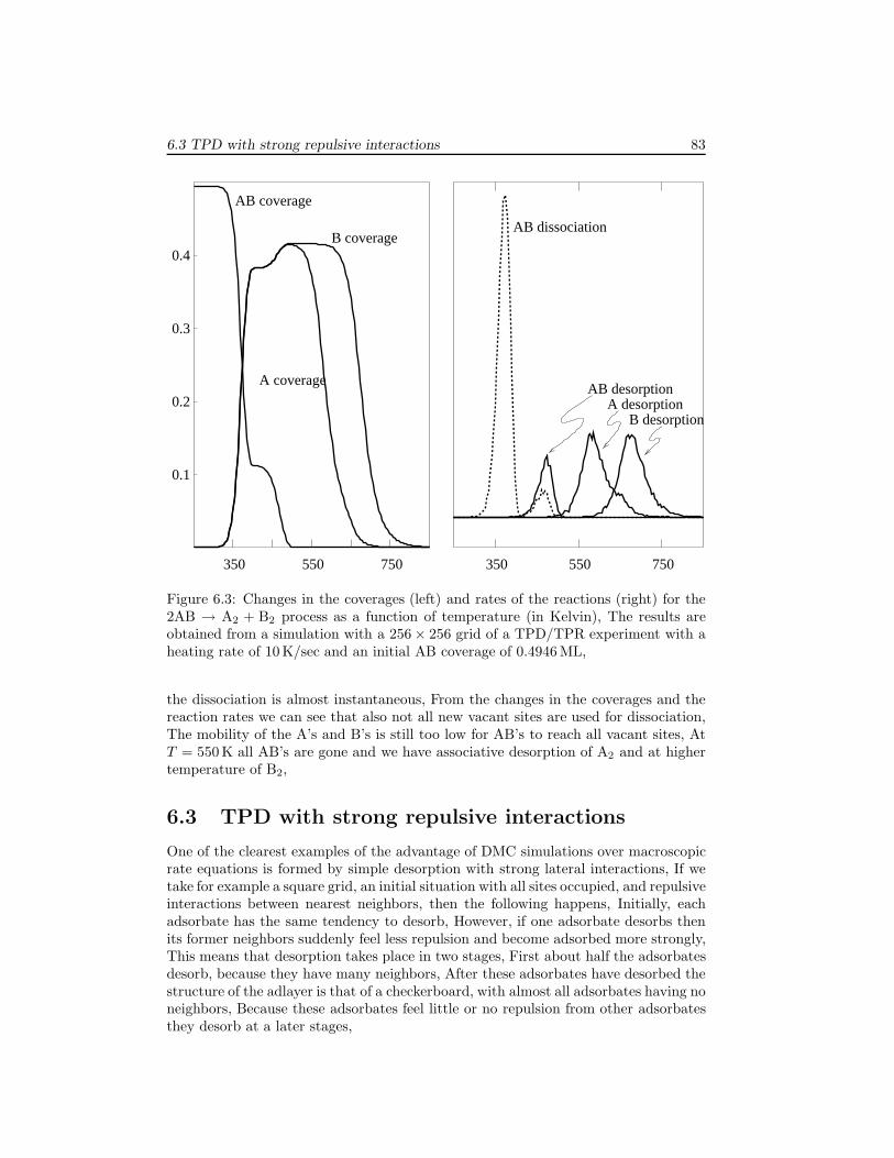
6.3 TPD with strong repulsive interactions 83
350 550 750 350 550 750
0.4
0.3
0.2
0.1
AB coverage
A coverage
B coverageAB dissociation
B desorptionA desorption
AB desorption
Figure 6.3: Changes in the coverages (left) and rates of the reactions (right) for the2AB → A2 + B2 process as a function of temperature (in Kelvin), The results areobtained from a simulation with a 256× 256 grid of a TPD/TPR experiment with aheating rate of 10 K/sec and an initial AB coverage of 0.4946 ML,
the dissociation is almost instantaneous, From the changes in the coverages and thereaction rates we can see that also not all new vacant sites are used for dissociation,The mobility of the A’s and B’s is still too low for AB’s to reach all vacant sites, AtT = 550 K all AB’s are gone and we have associative desorption of A2 and at highertemperature of B2,
6.3 TPD with strong repulsive interactions
One of the clearest examples of the advantage of DMC simulations over macroscopicrate equations is formed by simple desorption with strong lateral interactions, If wetake for example a square grid, an initial situation with all sites occupied, and repulsiveinteractions between nearest neighbors, then the following happens, Initially, eachadsorbate has the same tendency to desorb, However, if one adsorbate desorbs thenits former neighbors suddenly feel less repulsion and become adsorbed more strongly,This means that desorption takes place in two stages, First about half the adsorbatesdesorb, because they have many neighbors, After these adsorbates have desorbed thestructure of the adlayer is that of a checkerboard, with almost all adsorbates having noneighbors, Because these adsorbates feel little or no repulsion from other adsorbatesthey desorb at a later stages,
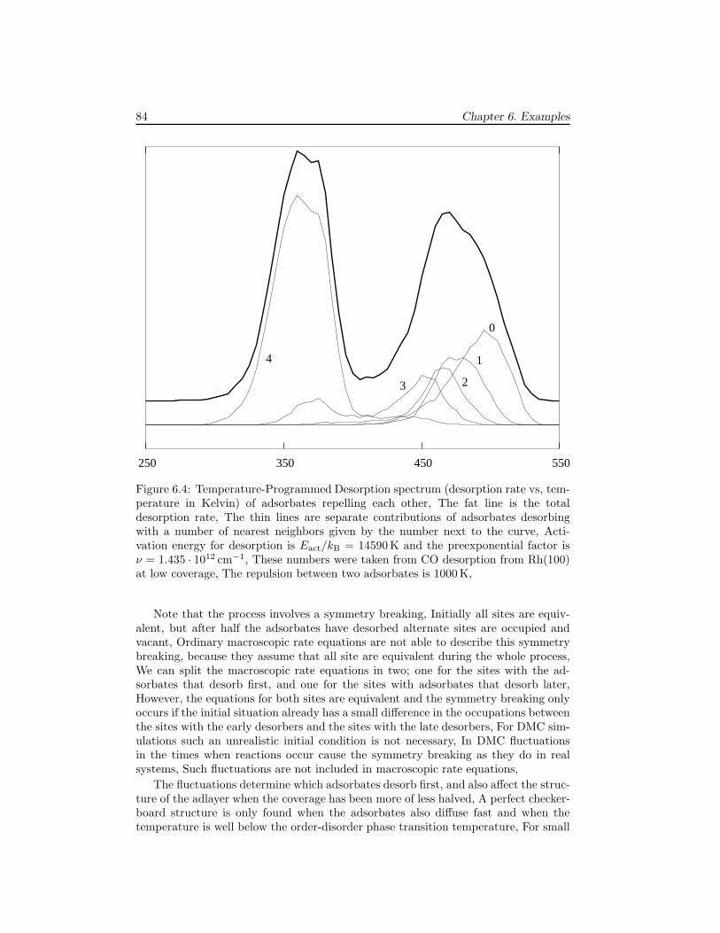
84 Chapter 6. Examples
4
3
250 350 450 550
2
1
0
Figure 6.4: Temperature-Programmed Desorption spectrum (desorption rate vs, tem-perature in Kelvin) of adsorbates repelling each other, The fat line is the totaldesorption rate, The thin lines are separate contributions of adsorbates desorbingwith a number of nearest neighbors given by the number next to the curve, Acti-vation energy for desorption is Eact/kB = 14590 K and the preexponential factor isν = 1.435 · 1012 cm−1, These numbers were taken from CO desorption from Rh(100)at low coverage, The repulsion between two adsorbates is 1000 K,
Note that the process involves a symmetry breaking, Initially all sites are equiv-alent, but after half the adsorbates have desorbed alternate sites are occupied andvacant, Ordinary macroscopic rate equations are not able to describe this symmetrybreaking, because they assume that all site are equivalent during the whole process,We can split the macroscopic rate equations in two; one for the sites with the ad-sorbates that desorb first, and one for the sites with adsorbates that desorb later,However, the equations for both sites are equivalent and the symmetry breaking onlyoccurs if the initial situation already has a small difference in the occupations betweenthe sites with the early desorbers and the sites with the late desorbers, For DMC sim-ulations such an unrealistic initial condition is not necessary, In DMC fluctuationsin the times when reactions occur cause the symmetry breaking as they do in realsystems, Such fluctuations are not included in macroscopic rate equations,
The fluctuations determine which adsorbates desorb first, and also affect the struc-ture of the adlayer when the coverage has been more of less halved, A perfect checker-board structure is only found when the adsorbates also diffuse fast and when thetemperature is well below the order-disorder phase transition temperature, For small
6.4 CO electrooxidation on a Pt-Ru electrode 85
system sizes the diffusion need not be so fast as for large system sizes, Diffusion hasto make sure that no domains are formed as in figure 5.9, Simulations show that evenat relatively small systems with say a 128 × 128 grid it is almost impossible to avoiddomain formation,
Figure 6.4 shows a TPD spectrum for a system with repulsive interactions, Weshow TPD instead of isothermal desorption, because the latter shows the two stagesin the desorption only in how fast the coverage and the desorption rate decreases, Ifthe coverage is plotted logarithmically, then we get first a straight line with a largenegative slope, followed by a straight line with a small, in absolute sense, negativeslope, In TPD the two stages are much clearer, because the desorption rate hastwo peaks, The figure shows that the second stage (i,e,, the second peak) has alsocontributions from adsorbates with one, two, and even three neighbors, which is dueto the fact that the first stage never forms a perfect checkerboard structure, If therepulsion becomes very strong, then more than two peaks can be formed,
In real systems the effects of lateral interactions are generally not so unambiguous,The lateral interactions have to be strong enough so that a well-defined structure isformed when half the adsorbates have desorbed, If this is not the case then the lateralinteractions only show up by shifting or broadening a single peak when the initialcoverage is increased, When lateral interactions are strong enough, then they mayalso push adsorbates to other adsorption sites, These sites have a lower adsorptionenergy, but overall the energy is lowered because it lessens the repulsion between theadsorbates, The result may even be an adlayer structure that is incommensurate withthe substrate, Finally, lateral interactions need not just be between nearest neighbors,Interactions between next- en next-next-nearest neighbors are not uncommon, Longerrange interactions have been excluded,[99] but charged adsorbates might have long-range interactions, which may explain very broad desorption peaks,
6.4 CO electrooxidation on a Pt-Ru electrode
The reason for doing DMC simulations is that the system is not homogeneous, Thismay be because the reactions cause an inhomogeneity in the adlayer, but it may alsobe that the substrate is inhomogeneous as in the case for the system of this section,The precise structure of the Pt-Ru electrode is not known, We will assume here thatthe two metals each form large islands mainly for illustrative purposes,[100] The ideaof having two metals is that each catalyzes only some reactions well, In the modelhere the CO2 formation proceeds well on Pt and the H2O dissociates on Ru,
We model the system with a square grid, We simulate a linear-sweep voltammetryexperiment in which the electrode is initially for 99% covered by CO, The followingreactions can occur,
H2O + ∗ → OH + H+ + e−,
OH + H+ + e− → H2O + ∗, (6.8)
CO + OH → CO2 + 2 ∗ +H+ + e−,
or if we just look at the site occupation
∗ → OH,
OH → ∗, (6.9)
CO + OH → 2∗,
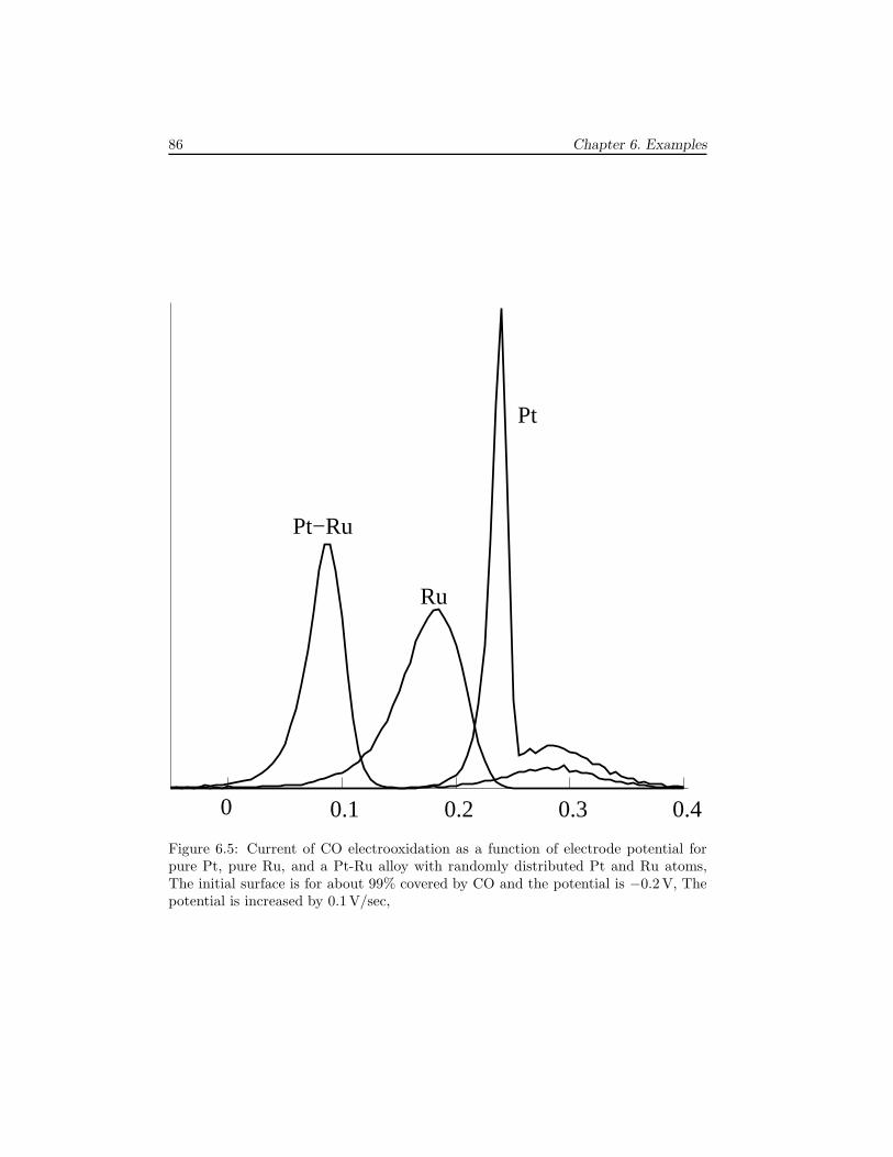
86 Chapter 6. Examples
0.1 0.2 0.3 0.4 0
Ru
Pt
Pt−Ru
Figure 6.5: Current of CO electrooxidation as a function of electrode potential forpure Pt, pure Ru, and a Pt-Ru alloy with randomly distributed Pt and Ru atoms,The initial surface is for about 99% covered by CO and the potential is −0.2 V, Thepotential is increased by 0.1 V/sec,
6.5 Oscillations of CO oxidation on Pt surfaces 87
The reactions can take place on both metals, and the latter also on the border of aPt and a Ru patch, The CO diffuses rapidly over the surface, whereas OH remainsfixed at the site where it is formed, In the experiment the current is measured; i,e,,the sum of the rates of the first and the last reaction minus the second,
Although the reactions can occur on both metals, the rate constants differ, Wecan write the rate constants as
WMads = kM
ads exp
[
αMe0E
kBT
]
,
WMdes = kM
des exp
[
− (1 − αM)e0E
kBT
]
, (6.10)
WM1M2
rx = kM1M2
rx exp
[
αM1M2e0E
kBT
]
,
The first refers to the dissociative adsorption of water, the second to the desorptionof water, and the last to the formation of CO2, In the last M1 is the metal with theCO, and M2 the metal with the OH, The α’s are so-called transfer coefficients, e0 isthe elementary charge, and E is the potential of the electrode, All transfer coefficientare taken equal to 0.5, T = 300 K, and kPt
ads = 0.2 s−1, kPtdes = 104 s−1, kRu
ads = 40 s−1,kRudes = 5 s−1, kRuRu
rx = 0.1 s−1, kRuPtrx = 0.1 s−1, kPtPt
rx = 1 s−1, and kPtRurx = 1 s−1, The
rate constant for CO diffusion is 100 s−1,Figure 6.5 shows the voltammograms for a Pt, a Ru, and a Pt-Ru electrode, These
are obtained by linearly changing the potential of the electrode from −0.2 to 0.5 Vin 7 seconds, The remarkable fact is that the Pt-Ru alloy is more reactive than eitherof the pure metals, The reason for this is as follows, The rate limiting step on Pt isthe dissociative adsorption of water, On Ru the rate limiting step is the formationof CO2, We get a synergetic effect if the oxidation step on the boundary of the Ptand Ru parts of the alloy is at least as fast as on Pt, In that case OH is formed onRu on the boundary, and CO on Pt reacts with this OH, This is most clearly seenwhen we do a simulation with large Pt and Ru islands (see figure 6.6), There is adepletion of CO on Pt near the boundary, because there the CO react, There is ahigher concentration of OH on Ru near the boundary because the higher oxidationreactivity there leads to more vacant sites for water adsorption,
6.5 Oscillations of CO oxidation on Pt surfaces
One problem for which extensive DMC simulations have been done by various groupsis the problem of CO oscillations on Pt(100) and Pt(110), A crucial role in theseoscillations is played by the reconstruction of the surface, and the effect of this re-construction on the adsorption of oxygen, The explanation of the oscillations is asfollows, A bare Pt surface reconstructs into a structure with a low sticking coefficientfor oxygen, This means that predominantly CO adsorbs on bare Pt, However, CO liftsthe reconstruction, The normal structure has a high sticking coefficient for oxygen,So after CO has adsorbed in a sufficient amount to lift the reconstruction oxygen canalso adsorb, The CO and the oxygen react, and form CO2, This CO2 rapidly desorbsleaving bare Pt which reconstructs again, An important aspect of this process, andalso other oscillatory reactions on surfaces, is the problem of synchronization, Thecycle described above can easily take place on the whole surface, but oscillations on
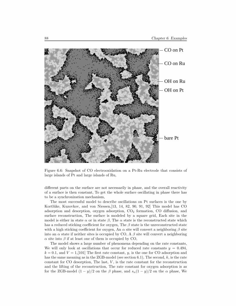
88 Chapter 6. Examples
CO on Pt
CO on Ru
OH on Ru
OH on Pt
bare Pt
Figure 6.6: Snapshot of CO electrooxidation on a Pt-Ru electrode that consists oflarge islands of Pt and large islands of Ru,
different parts on the surface are not necessarily in phase, and the overall reactivityof a surface is then constant, To get the whole surface oscillating in phase there hasto be a synchronization mechanism,
The most successful model to describe oscillations on Pt surfaces is the one byKortluke, Kuzovkov, and von Niessen,[13, 14, 82, 90, 91, 92] This model has COadsorption and desorption, oxygen adsorption, CO2 formation, CO diffusion, andsurface reconstruction, The surface is modeled by a square grid, Each site in themodel is either in state α or in state β, The α state is the reconstructed state whichhas a reduced sticking coefficient for oxygen, The β state is the unreconstructed statewith a high sticking coefficient for oxygen, An α site will convert a neighboring β siteinto an α state if neither sites is occupied by CO, A β site will convert a neighboringα site into β if at least one of them is occupied by CO,
The model shows a large number of phenomena depending on the rate constants,We will only look at oscillations that occur for reduced rate constants y = 0.494,k = 0.1, and V = 1,[101] The first rate constant, y, is the one for CO adsorption andhas the same meaning as in the ZGB-model (see section 6.1), The second, k, is the rateconstant for CO desorption, The last, V , is the rate constant for the reconstructionand the lifting of the reconstruction, The rate constant for oxygen adsorption is asfor the ZGB-model (1 − y)/2 on the β phase, and sα(1 − y)/2 on the α phase, We
6.5 Oscillations of CO oxidation on Pt surfaces 89
will look at the Pt(110) surface which has sα = 0.5, The diffusion rate constant hasbeen varied,
Figure 6.7 shows snapshots obtained from some large simulations in which thediffusion is just about fast enough to lead to global oscillations provided the initialconditions are favorable, However, it is also possible to choose the initial conditionsso that the oscillations are not synchronized properly, In that case one can see theformation of patterns as the right half of the figure shows,
Synchronization is obtained when the diffusion rate is fast enough, The minimalvalue is related to the so-called Turing-like structures that are formed in the substrate,These structure can best be seen in the lower two pictures on the left and all pictureson the right of figure 6.7, If diffusion is so fast that within one oscillatory period COcan move from one phase (α or β) to a neighboring island of the other phase, then theoscillation are well synchronized, If the diffusion rate is slower, then we get patternformation, Note that the system has two length scales, The characteristic length scaleof the adlayer is much larger than the characteristic length scale of the Turing-likestructures as can be seen in the right half of the figure,
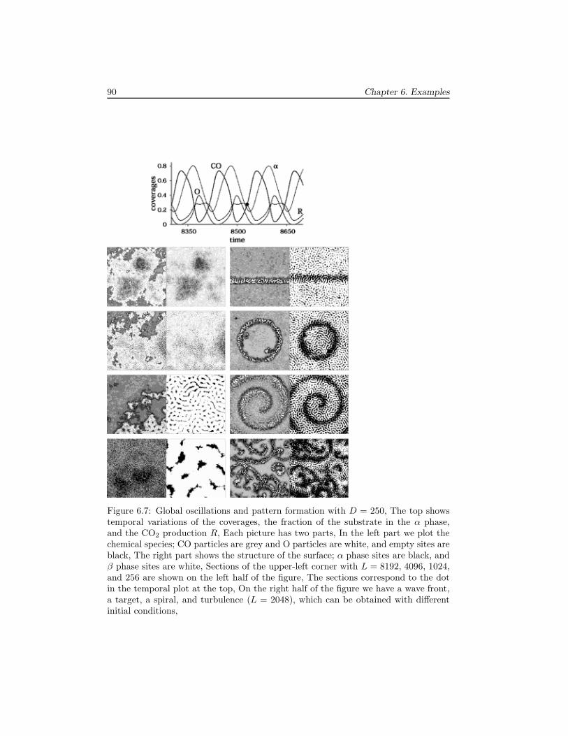
90 Chapter 6. Examples
Figure 6.7: Global oscillations and pattern formation with D = 250, The top showstemporal variations of the coverages, the fraction of the substrate in the α phase,and the CO2 production R, Each picture has two parts, In the left part we plot thechemical species; CO particles are grey and O particles are white, and empty sites areblack, The right part shows the structure of the surface; α phase sites are black, andβ phase sites are white, Sections of the upper-left corner with L = 8192, 4096, 1024,and 256 are shown on the left half of the figure, The sections correspond to the dotin the temporal plot at the top, On the right half of the figure we have a wave front,a target, a spiral, and turbulence (L = 2048), which can be obtained with differentinitial conditions,
Bibliography
[1] M. P. Allen and D. J. Tildesley, Computer Simulation of Liquids (Clarendon,Oxford, 1987).
[2] A. Zangwill, Physics at Surfaces (Cambridge University Press, Cambridge,1988).
[3] J. M. Thomas and W. J. Thomas, Principles and Practice of Heterogeneous
Catalysis (VCH, Weinheim, 1997).
[4] N. W. Ashcroft and N. D. Mermin, Solid State Physics (Holt, Rinehart, andWinston, New York, 1976).
[5] N. V. Petrova and I. N. Yakovkin, Lateral Interaction and CO Adlayer Struc-tures on the Pt(111) Surface, Surf. Sci. 519 (2002) 90.
[6] C.-T. Kao, G. S. Blackman, M. A. V. Hove, G. A. Somorjai, and C.-M.Chan, The Surface Structure and Chemical Reactivity of Rh(111)-(2×2)-3NOby HREELS and Dynamical LEED Analysis, Surf. Sci. 224 (1989) 77.
[7] M. van Hardeveld, Elementary Reactions in the Catalytic Reduction of NO on
Rhodium Surfaces , Ph.D. thesis, Eindhoven University of Technology (1997).
[8] S. Dahl, A. Logadottir, R. C. Egeberg, J. H. Larsen, I. Chorkendorff,E. Tornqvist, and J. K. N. rskov. Role of Steps in N2 Activation on Ru(0001),Phys. Rev. Lett. 83 (1999) 1814.
[9] B. Hammer, Bond Activation at Monatomic Steps: NO Dissociation at Corru-gated Ru(0001), Phys. Rev. Lett. 83 (2000) 3681.
[10] R. Imbihl and G. Ertl, Oscillatory Kinetics in Heterogeneous Catalysis, Chem.
Rev. 95 (1995) 697.
[11] M. M. Slin’ko and N. I. Jaeger, Oscillating Heterogeneous Catalytic Systems,
Studies in Surface Science and Catalysis 86 (Elsevier, Amsterdam, 1994).
[12] R. J. Gelten, A. P. J. Jansen, R. A. van Santen, J. J. Lukkien, J. P. L, Segers,and P. A. J. Hilbers. Monte Carlo Simulations of a Surface Reaction ModelShowing Spatio-Temporal Pattern Formation and Oscillations, J. Chem. Phys.
108 (1998) 5921.
[13] V. N. Kuzovkov, O. Kortlucke, and W. von Niessen, Nucleation and IslandGrowth Kinetics on Reconstructing Surfaces, Phys. Rev. Lett. 83 (1999) 1636.
91
92 BIBLIOGRAPHY
[14] O. Kortlucke, V. N. Kuzovkov, and W. von Niessen, Global Synchronization viaHomogeneous Nucleation in Oscillating Surface Reactions, Phys. Rev. Lett. 83(1999) 3089.
[15] M. Gruyters, T. Ali, and D. A. King, Modelling temporal kinetic oscillations forCO oxidation on Pt100. The (1×1)-CO island growth rate power law model,Chem. Phys. Lett. 232 (1995) 1.
[16] M. Gruyters, T. Ali, and D. A. King, Theoretical inquiry into the microscopicorigins of the oscillatory CO oxidation reaction on Pt100, J. Phys. Chem.
100 (1996) 14417.
[17] A. R. Leach, Molecular Modelling. Principles and Applications (Longman, Sin-gapore, 1996).
[18] J. C. Keck, Variational Theory of Chemical Reaction Rates Applied to Three-Body Recombinations, J. Chem. Phys. 32 (1960) 1035.
[19] J. C. Keck, Statistical Investigation of Dissociation Cross-Section for Diatoms,Discuss. Faraday Soc. 33 (1962) 173.
[20] J. C. Keck, Variational Theory of Reaction Rates, Adv. Chem. Phys. 13 (1967)85.
[21] P. Pechukas, Statistical Approximations in Collision Theory, In W. Miller (ed.),Dynamics of Molecular Collisions, Part B , 269–322 (Plenum Press, New York,1976).
[22] D. G. Truhlar, A. D. Isaacson, and B. C. Garrett, Generalized Transition StateTheory, In M. Baer (ed.), Theory of Chemical Reaction Dynamics, Part IV ,65–138 (CRC Press, Boca Raton, 1985).
[23] W. H. Miller, Quantum Mechanical Transition State Theory and a New Semi-classical Model for Reaction Rate Constants, J. Chem. Phys. 61 (1974) 1823.
[24] W. H. Miller, Semiclassical Limit of Quantum Mechanical Transition State The-ory for Nonseparable Systems, J. Chem. Phys. 62 (1975) 1899.
[25] G. A. Voth, Feynman Path Integral Formulation of Quantum MechanicalTransition-State Theory, J. Phys. Chem. 97 (1993) 8365.
[26] V. A. Benderskii, D. E. Makarov, and C. A. Wight, Chemical Dynamics at LowTemperatures, Adv. Chem. Phys. 88 (1994) 1.
[27] D. A. McQuarrie, Statistical Mechanics (Harper, New York, 1976).
[28] R. Becker, Theorie der Warme (Springer, Berlin, 1985).
[29] A. P. J. Jansen, Compensating Hamiltonian Method for Chemical ReactionDynamics: Xe Desorption from Pd(100), J. Chem. Phys. 94 (1991) 8444.
[30] E. Kreyszig, Advanced Engineering Mathematics (Wiley, New York, 1993).
[31] A. H. Zemanian, Distribution Theory and Transform Analysis (Dover, NewYork, 1987).
BIBLIOGRAPHY 93
[32] R. A. van Santen and J. W. Niemantsverdriet, Chemical Kinetics and Catalysis
(Plenum Press, New York, 1995).
[33] P. G. Mezey, Potential Energy Hypersurfaces (Elsevier, Amsterdam, 1987).
[34] E. K. Grimmelmann, J. C. Tully, and E. Helfand, Molecular Dynamics of In-frequent Events: Thermal Desorption of Xenon from a Platinum Surface, J.
Chem. Phys. 74 (1981) 5300.
[35] J. C. Tully, Dynamics of gas-surface interactions: Thermal desorption of Ar andXe from platinum, Surf. Sci. 111 (1981) 461.
[36] E. B.Wilson, J. C. Decius, and P. C. Cross, Molecular Vibrations: The Theory
of Infrared and Raman Vibrational Spectra (McGraw-Hill, London, 1955).
[37] H. Goldstein, Classical Mechanics (Addison-Wesley, Amsterdam, 1981).
[38] A. Messiah, Quantum Mechanics (North-Holland, Amsterdam, 1961).
[39] P. Hohenberg and W. Kohn, Inhomogeneous Electron Gas, Phys. Rev. 136(1964) B864.
[40] W. Kohn and L. S. Sham, Self-Consistent Equations Including Exchange andCorrelation Effects, Phys. Rev. 140 (1965) A1133.
[41] R. G. Parr and W. Yang, Density-Functional Theory of Atoms and Molecules
(Oxford University Press, New York, 1989).
[42] M. Abramowitz and I. A. Stegun, Handbook of Mathematical Functions with
Formulas, Graphs, and Mathematical Tables (Dover, New York, 1965).
[43] A. P. J. Jansen, Monte Carlo Simulations of Chemical Reactions on a Sur-face with Time-Dependent Reaction-Rate Constants, Comput. Phys. Comm.
86 (1995) 1.
[44] A. M. de Jong and J. W. Niemantsverdriet, Thermal desorption analysis: Com-parative test of ten commonly applied procedures, Surf. Sci. 233 (1990) 355.
[45] G. A. Somorjai, Introduction to surface chemistry and catalysis (Wiley, Chich-ester, 1993).
[46] A. Cassuto and D. A. King, Rate Expressions for Adsorption and DesorptionKinetics with Precursor States and Lateral Interactions, Surf. Sci. 102 (1981)388.
[47] K. Binder, Monte Carlo Methods in Statistical Physics (Springer, Berlin, 1986).
[48] D. T. Gillespie, A general method for numerically simulating the stochastic timeevolution of coupled chemical reactions, J. Comput. Phys. 22 (1976) 403.
[49] D. T. Gillespie, Exact stochastic simulations of coupled chemical reactions, J.
Phys. Chem. 81 (1977) 2340.
[50] J. Honerkamp, Stochastische Dynamische Systeme (VCH, Weinheim, 1990).
94 BIBLIOGRAPHY
[51] A. P. J. Jansen and J. J. Lukkien, Dynamic Monte-Carlo Simulations of Reac-tions in Heterogeneous Catalysis, Catalysis Today 53 (1999) 259.
[52] D. T. Gillespie, Approximate Accelerated Stochastic Simulation of ChemicallyReacting Systems, J. Chem. Phys. 115 (2001) 1716.
[53] H. Resat, H. S. Wiley, and D. A. Dixon, Probability Weighted Dynamic MonteCarlo Method for Reaction Kinetics Simulations. Submitted to J. Chem. Phys.B (2001).
[54] K. A. Fichthorn and W. H. Weinberg, Theoretical Foundations of DynamicalMonte Carlo Simulations, J. Chem. Phys. 95 (1991) 1090.
[55] H. C. Kang and W. H. Weinberg, Kinetic modeling of surface rate processes,Surf. Sci. 299/300 (1994) 755.
[56] B. Meng and W. H. Weinberg, Monte Carlo Simulations of Temperature-Programmed Desorption Spectra, J. Chem. Phys. 100 (1994) 5280.
[57] F. C. Alcaraz, M. Droz, M. Henkel, and V. Rittenberg, Reaction-Diffusion Pro-cesses, Critical Dynamics, and Quantum Chains, J. Phys. 230 (1994) 250.
[58] W. Feller, An Introduction to Probability Theory and Its Applications (Wiley,New York, 1970).
[59] D. E. Knuth, The Art of Computer Programming, Volume III: Sorting and
Searching (Addison-Wesley, Reading, 1973).
[60] I. Mitrani, Simulation Techniques for Discrete Event Systems (Cambridge Uni-versity Press, Cambridge, 1982).
[61] J. J. Lukkien, J. P. L. Segers, P. A. J. Hilbers, R. J. Gelten, and A. P. J,Jansen. Efficient Monte Carlo Methods for the Simulation of Catalytic SurfaceReactions, Phys. Rev. E 58 (1998) 2598.
[62] J. P. L. Segers, Algorithms for the Simulation of Surface Processes. Ph.D. thesis,Eindhoven University of Technology (1999).
[63] D. E. Knuth, The Art of Computer Programming, Volume I: Fundamental Al-
gorithms (Addison-Wesley, Reading, 1973).
[64] A. P. J. Jansen, A Monte Carlo Study of Temperature-Programmed DesorptionWith Lateral Attractive Interactions, Phys. Rev. B 52 (1995) 5400.
[65] R. M. Nieminen and A. P. J. Jansen, Monte Carlo Simulations of Surface Re-actions, Appl. Catal. A: General 160 (1997) 99.
[66] M. T. M. Koper, J. J. Lukkien, A. P. J. Jansen, P. A. J. Hilbers, and R. A.va, Santen. Monte Carlo Simulations of a Simple Model for the ElectrocatalyticCO Oxidation on Platinum, J. Chem. Phys. 109 (1998) 6051.
[67] S. J. Lombardo and A. T. Bell, A Review of Theoretical Models of Adsorption,Diffusion, Desorption, and Reaction of Gases on Metal Surfaces, Surf. Sci. Rep.
13 (1991) 1.
BIBLIOGRAPHY 95
[68] V. Privman, Nonequilibrium Statistical Mechanics in One Dimension (Cam-bridge University Press, Cambridge, 1997).
[69] J. Mai and W. von Niessen, Cellular-automaton approach to a surface reaction,Phys. Rev. A 44 (1991) R6165.
[70] J. Mai and W. von Niessen, Diffusion and reaction in multicomponent systemsvia cellular-automaton modeling: A + B2, J. Chem. Phys. 98 (1993) 2032.
[71] R. Danielak, A. Perera, M. Moreau, M. Frankowicz, and R. Kapral, SurfaceStructure and Catalytic CO Oxidation Oscillations, Physica A 229 (1996) 428.
[72] J. P. Boon, B. Dab, R. Kapral, and A. Lawniczak, Lattice Gas Automata forReactive Systems, Phys. Rep. 273 (1996) 55.
[73] J. R. Weimar, Simuation with Cellular Automata (Logos Verlag, Berlin, 1997).
[74] S. Wolfram, A New Kind of Science (Wolfram Media, Champaign, Illinois,2002).
[75] B. Drossel, Self-Organized Criticality and Synchronization in the Forest-Fire Model, Los Alamos Preprint Server; http://xxx.lanl.gov, paperno.cond-mat/9506021 (1995).
[76] CARLOS is a general-purpose program, written in C by J. J. Lukkien, fo,simulating reactions on surfaces that can be represented by regular grids; animplementation of the First-Reaction Method, the Variable Stepsize Method,and the Random Selection Method, http://wwwpa.win.tue.nl/johanl/carlos/.
[77] W. H. Press, B. P. Flannery, S. A. Teukolsky, and W. T. Vetterling, Numerical
Recipes. The Art of Scientific Computing (Cambridge University Press, Cam-bridge, 1989).
[78] J. Stoer and R. Bulirsch, Introduction to Numerical Analysis (Springer, NewYork, 1993).
[79] S. Redner, Scaling Theories of Diffusion-Controlled and Ballistically ControlledBimolecular Reactions, In V. Privman (ed.), Nonequilibrium Statistical Mechan-
ics in One Dimension, 3–27 (Cambridge University Press, Cambridge, 1996).
[80] A. A. Ovchinnikov and Y. B. Zeldovich, Role of Density Fluctuations in Bi-molecular Reaction Kinetics, Chem. Phys. 28 (1978) 215.
[81] D. Toussaint and F. Wilczek, Particle-Antiparticle Annihilation in DiffusiveMotion, J. Chem. Phys. 78 (1983) 2642.
[82] V. N. Kuzovkov, O. Kortlucke, and W. von Niessen, Kinetic Model for SurfaceReconstruction, Phys. Rev. E 66 (2002) 011603.
[83] V. P. Zhdanov and B. Kasemo, ??, J. Catal. 170 (1997) 377.
[84] V. P. Zhdanov and B. Kasemo, Kinetics of the 2A+B → 2AB Reaction Compli-cated by Spatial Constraints for Adsorption, Formation of Islands, and Steps,Surf. Sci. 412/413 (1998) 527.
96 BIBLIOGRAPHY
[85] R. M. Ziff, E. Gulari, and Y. Barshad, Kinetic Phase Transitions in an Irre-versible Surface-Reaction Model, Phys. Rev. Lett. 56 (1986) 2553.
[86] H.-P. Kaukonen and R. M. Nieminen, Computer simulation studies of the cat-alytic oxidation of carbon monoxide on platinum metals, J. Chem. Phys. 91(1989) 4380.
[87] J.-P. Hovi, J. Vaari, H.-P. Kaukonen, and R. M. Nieminen, Simulations of theeffect of preadsorbed poisons and promoters on irreversible surface reactions,Comput. Mater. Sci. 1 (1992) 33.
[88] J. Mai, A. Casties, W. von Niessen, and V. N. Kuzovkov, A Stochastic Modeland a Monte Carlo Simulation for the Description of CO Oxidation on Pt/SnAlloys, J. Chem. Phys. 102 (1995) 5037.
[89] R. J. Gelten, R. A. van Santen, and A. P. J. Jansen, Dynamic Monte CarloSimulations of Oscillatory Heterogeneous Catalytic Reactions, In P. B. Balbuenaand J. M. Seminario (eds.), Molecular Dynamics: From Classical to Quantum
Methods (Elsevier, Amsterdam, 1999).
[90] O. Kortlucke, V. N. Kuzovkov, and W. von Niessen, Oscillation PhenomenaLeading to Chaos in a Stochastic Surface Reaction Model, Phys. Rev. Lett. 81(1998) 2164.
[91] V. N. Kuzovkov, O. Kortlucke, and W. von Niessen, Kinetic Oscillations in theCatalytic CO Oxidation on Pt Single Crystal Surfaces: Theory and Simulations,J. Chem. Phys. 108 (1998) 5571.
[92] O. Kortlucke, V. N. Kuzovkov, and W. von Niessen, Simulation of KineticOscillations in Surface Reactions on Reconstructing Surfaces, J. Chem. Phys.
110 (1999) 11523.
[93] N. M. H. Janssen, P. D. Cobden, and B. E. Nieuwenhuys, Non-linear behaviourof nitric oxide reduction reactions over metal surfaces, J. Phys. Condens. Matter
9 (1997) 1889.
[94] R. M. Ziff and B. J. Brosilow, Investigation of the first-order phase transitionin the A−B2 reaction model using a constant-coverage kinetic ensemble, Phys.
Rev. A 46 (1992) 4630.
[95] B. J. Brosilow, E. Gulari, and R. M. Ziff, Boundary effects in a surface reactionmodel for CO oxidation, J. Chem. Phys. 98 (1993) 674.
[96] I. Jensen, H. Fogedby, and R. Dickman, Critical Exponents for an IrreversibleSurface Reaction Model, Phys. Rev. A 41 (1990) 3411.
[97] R. M. van Hardeveld, M. J. P. Hopstaken, J. J. Lukkien, P. A. J. Hilbers, A. P. J.Jansen, R. A. van Santen, and J. W. Niemantsverdriet. Role of Surface Diffusionin the Ordering of Adsorbed Molecules: Dynamic Monte Carlo Simulations ofNO on Rh(111), Chem. Phys. Lett. 302 (1999) 98.
BIBLIOGRAPHY 97
[98] A. P. J. Jansen, C. G. M. Hermse, F. Frechard, and J. J. Lukkien, Ab-initiokinetics of heterogeneous catalysis: NO+N+O/Rh(111). In V. Alexandrov,J. Dongarra, B. Juliano, R. Renner, and C. Ta, (eds.), Computational Science—
ICCS 2001 , 531–540 (Springer, Berlin, 2001).
[99] Q. Ge, R. Kose, and D. A. King, Adsorption Energetics and Bonding fromFemtomole Calorimetry and from First Principles Theory, Adv. Catal. 45 (2000)207.
[100] M. T. M. Koper, J. J. Lukkien, A. P. J. Jansen, and R. A. van Santen, LatticeGas Model for CO Electrooxidation on Pt-Ru Bimetallic Surfaces, J. Phys.
Chem. B 103 (1999) 5522.
[101] R. Salazar, A. P. J. Jansen, and V. N. Kuzovkov, A New Synchronization Mech-anism Via Turing-Like Microscopic Structures for CO Oxidation on Pt(110), LosAlamos Preprint Server; http://arXiv.org/, paperno. cond-mat/0210699 (2002).