
Fpga based implementation of a double precision ieee floating point adder

J.1 Introduction J-2
J.2 Basic Techniques of Integer Arithmetic J-2
J.3 Floating Point J-13
J.4 Floating-Point Multiplication J-17
J.5 Floating-Point Addition J-21
J.6 Division and Remainder J-27
J.7 More on Floating-Point Arithmetic J-32
J.8 Speeding Up Integer Addition J-37
J.9 Speeding Up Integer Multiplication and Division J-44
J.10 Putting It All Together J-57
J.11 Fallacies and Pitfalls J-62
J.12 Historical Perspective and References J-63
Exercises J-67
J
Computer Arithmeticby David Goldberg
Xerox Palo Alto Research CenterThe Fast drives out the Slow even if the Fast is wrong.
W. Kahan
J-2 ■ Appendix J Computer Arithmetic
J.1
J.2
Introduction
Although computer arithmetic is sometimes viewed as a specialized part of CPUdesign, it is a very important part. This was brought home for Intel in 1994 whentheir Pentium chip was discovered to have a bug in the divide algorithm. Thisfloating-point flaw resulted in a flurry of bad publicity for Intel and also cost thema lot of money. Intel took a $300 million write-off to cover the cost of replacingthe buggy chips.
In this appendix, we will study some basic floating-point algorithms, includ-ing the division algorithm used on the Pentium. Although a tremendous varietyof algorithms have been proposed for use in floating-point accelerators, actualimplementations are usually based on refinements and variations of the few basicalgorithms presented here. In addition to choosing algorithms for addition, sub-traction, multiplication, and division, the computer architect must make otherchoices. What precisions should be implemented? How should exceptions behandled? This appendix will give you the background for making these and otherdecisions.
Our discussion of floating point will focus almost exclusively on the IEEEfloating-point standard (IEEE 754) because of its rapidly increasing acceptance.Although floating-point arithmetic involves manipulating exponents and shiftingfractions, the bulk of the time in floating-point operations is spent operating onfractions using integer algorithms (but not necessarily sharing the hardware thatimplements integer instructions). Thus, after our discussion of floating point,we will take a more detailed look at integer algorithms.
Some good references on computer arithmetic, in order from least to mostdetailed, are Chapter 3 of Patterson and Hennessy [2009]; Chapter 7 of Hamacher,
Vranesic, and Zaky [1984]; Gosling [1980]; and Scott [1985].Basic Techniques of Integer Arithmetic
Readers who have studied computer arithmetic before will find most of this sectionto be review.
Ripple-Carry Addition
Adders are usually implemented by combining multiple copies of simple com-ponents. The natural components for addition are half adders and full adders.The half adder takes two bits a and b as input and produces a sum bit s and acarry bit cout as output. Mathematically, s¼ (a+b) mod 2, and cout¼b(a+b)/2c,where b c is the floor function. As logic equations, s¼ ab + ab and cout¼ab,where ab means a ^ b and a+b means a _ b. The half adder is also called
a (2,2) adder, since it takes two inputs and produces two outputs. The full adder
J:2:1
J:2:2
J.2 Basic Techniques of Integer Arithmetic ■ J-3
is a (3,2) adder and is defined by s¼ (a+b+c) mod 2, cout¼b(a+b+c)/2c, orthe logic equations
s¼ abc+ abc+ abc+ abc
cout ¼ ab+ ac + bc
The principal problem in constructing an adder for n-bit numbers out of smallerpieces is propagating the carries from one piece to the next. The most obviousway to solve this is with a ripple-carry adder, consisting of n full adders, asillustrated in Figure J.1. (In the figures in this appendix, the least-significantbit is always on the right.) The inputs to the adder are an�1an�2⋯a0and bn�1bn�2⋯b0, where an�1an�2⋯a0 represents the numberan�12n�1 + an�22n�2 +⋯+ a0. The ci+1 output of the ith adder is fed into the ci + 1
input of the next adder (the (i+1)-th adder) with the lower-order carry-in c0set to 0. Since the low-order carry-in is wired to 0, the low-order adder could be a halfadder. Later, however, we will see that setting the low-order carry-in bit to 1 is usefulfor performing subtraction.
In general, the time a circuit takes to produce an output is proportional to themaximum number of logic levels through which a signal travels. However, deter-mining the exact relationship between logic levels and timings is highly technologydependent. Therefore, when comparing adders we will simply compare the numberof logic levels in each one. How many levels are there for a ripple-carry adder? Ittakes two levels to compute c1 from a0 and b0. Then it takes two more levels to com-pute c2 from c1, a1, b1, and so on, up to cn. So, there are a total of 2n levels. Typicalvalues of n are 32 for integer arithmetic and 53 for double-precision floating point.The ripple-carry adder is the slowest adder, but also the cheapest. It can be built withonly n simple cells, connected in a simple, regular way.
Because the ripple-carry adder is relatively slow compared with the designsdiscussed in Section J.8, you might wonder why it is used at all. In technologieslike CMOS, even though ripple adders take time O(n), the constant factor is verysmall. In such cases short ripple adders are often used as building blocks in larger
adders.bn–1
an–1
sn–1
Fulladder
cn–1
sn–2
cn
an–2
bn–2
Fulladder
b1
a1
s1
Fulladder
s0
a0
b0
Fulladder
c2 c
1
0
Figure J.1 Ripple-carry adder, consisting of n full adders. The carry-out of one fulladder is connected to the carry-in of the adder for the next most-significant bit. Thecarries ripple from the least-significant bit (on the right) to the most-significant bit(on the left).

Multiply Step
J-4 ■ Appendix J Computer Arithmetic
Radix-2 Multiplication and Division
The simplest multiplier computes the product of two unsigned numbers, one bit at atime, as illustrated in Figure J.2(a). The numbers to be multiplied are an�1an�2⋯a0and bn�1bn�2⋯b0, and they are placed in registers A and B, respectively. Register
P is initially 0. Each multiply step has two parts:(i) If the least-significant bit of A is 1, then register B, containing bn�1bn�2⋯b0, isadded to P; otherwise, 00⋯00 is added to P. The sum is placed back into P.
(ii) Registers P and A are shifted right, with the carry-out of the sum being movedinto the high-order bit of P, the low-order bit of P being moved into register A,and the rightmost bit of A, which is not used in the rest of the algorithm, being
shifted out.Carry-out
AP
n
n
n
Shift
P
B0
A
n + 1
n1
n
Shift
(a)
(b)
1
B
Figure J.2 Block diagram of (a) multiplier and (b) divider for n-bit unsigned integers.Each multiplication step consists of adding the contents of P to either B or 0 (dependingon the low-order bit of A), replacing P with the sum, and then shifting both P and A onebit right. Each division step involves first shifting P and A one bit left, subtracting B fromP, and, if the difference is nonnegative, putting it into P. If the difference is nonnegative,the low-order bit of A is set to 1.
Divide Step
Nonrestoring
Divide Step
J.2 Basic Techniques of Integer Arithmetic ■ J-5
After n steps, the product appears in registers P and A, with A holding thelower-order bits.
The simplest divider also operates on unsigned numbers and produces thequotient bits one at a time. A hardware divider is shown in Figure J.2(b). Tocompute a/b, put a in the A register, b in the B register, and 0 in the P register
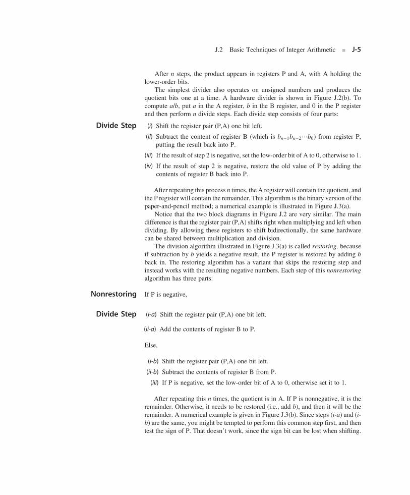
and then perform n divide steps. Each divide step consists of four parts:(i) Shift the register pair (P,A) one bit left.
(ii) Subtract the content of register B (which is bn�1bn�2⋯b0) from register P,putting the result back into P.
(iii) If the result of step 2 is negative, set the low-order bit of A to 0, otherwise to 1.
(iv) If the result of step 2 is negative, restore the old value of P by adding thecontents of register B back into P.
After repeating this process n times, the A register will contain the quotient, andthe P register will contain the remainder. This algorithm is the binary version of thepaper-and-pencil method; a numerical example is illustrated in Figure J.3(a).
Notice that the two block diagrams in Figure J.2 are very similar. The maindifference is that the register pair (P,A) shifts right when multiplying and left whendividing. By allowing these registers to shift bidirectionally, the same hardwarecan be shared between multiplication and division.
The division algorithm illustrated in Figure J.3(a) is called restoring, becauseif subtraction by b yields a negative result, the P register is restored by adding bback in. The restoring algorithm has a variant that skips the restoring step andinstead works with the resulting negative numbers. Each step of this nonrestoring
algorithm has three parts:If P is negative,
(i-a) Shift the register pair (P,A) one bit left.
(ii-a) Add the contents of register B to P.
Else,
(i-b) Shift the register pair (P,A) one bit left.
(ii-b) Subtract the contents of register B from P.
(iii) If P is negative, set the low-order bit of A to 0, otherwise set it to 1.
After repeating this n times, the quotient is in A. If P is nonnegative, it is theremainder. Otherwise, it needs to be restored (i.e., add b), and then it will be theremainder. A numerical example is given in Figure J.3(b). Since steps (i-a) and (i-b) are the same, you might be tempted to perform this common step first, and then
test the sign of P. That doesn’t work, since the sign bit can be lost when shifting.
Figure J.3 Numerical example of (a) restoring division and (b) nonrestoring division.
J-6 ■ Appendix J Computer Arithmetic

Example
Answer
J.2 Basic Techniques of Integer Arithmetic ■ J-7
The explanation for why the nonrestoring algorithm works is this. Let rk be thecontents of the (P,A) register pair at step k, ignoring the quotient bits (which are sim-ply sharing the unused bits of register A). In Figure J.3(a), initially A contains 14, sor0¼14. At the end of the first step, r1¼28, and so on. In the restoring algorithm, part(i) computes 2rk and then part (ii) 2rk�2nb (2nb since b is subtracted from the lefthalf). If 2rk�2nb�0, both algorithms end the step with identical values in (P,A). If2rk�2nb<0, then the restoring algorithm restores this to 2rk, and the next stepbegins by computing rres¼2(2rk)�2nb. In the non-restoring algorithm, 2rk�2nbis kept as a negative number, and in the next step rnonres¼2(2rk�2nb)+2nb¼4rk�2nb¼ rres. Thus (P,A) has the same bits in both algorithms.
If a and b are unsigned n-bit numbers, hence in the range 0�a,b�2n�1, thenthe multiplier in Figure J.2 will work if register P is n bits long. However, fordivision, P must be extended to n+1 bits in order to detect the sign of P. Thusthe adder must also have n+1 bits.
Why would anyone implement restoring division, which uses the same hard-ware as nonrestoring division (the control is slightly different) but involves an extraaddition? In fact, the usual implementation for restoring division doesn’t actuallyperform an add in step (iv). Rather, the sign resulting from the subtraction is testedat the output of the adder, and only if the sum is nonnegative is it loaded back intothe P register.
As a final point, before beginning to divide, the hardware must check to seewhether the divisor is 0.
Signed Numbers
There are four methods commonly used to represent signed n-bit numbers: signmagnitude, two’s complement, one’s complement, and biased. In the sign magni-tude system, the high-order bit is the sign bit, and the low-order n�1 bits are themagnitude of the number. In the two’s complement system, a number and itsnegative add up to 2n. In one’s complement, the negative of a number is obtainedby complementing each bit (or, alternatively, the number and its negative add up to2n�1). In each of these three systems, nonnegative numbers are represented in theusual way. In a biased system, nonnegative numbers do not have their usual rep-resentation. Instead, all numbers are represented by first adding them to the biasand then encoding this sum as an ordinary unsigned number. Thus, a negative num-ber k can be encoded as long as k+bias�0. A typical value for the bias is 2n�1.
Using 4-bit numbers (n¼4), if k¼3 (or in binary, k¼00112), how is�k expressed
in each of these formats?In signed magnitude, the leftmost bit in k¼00112 is the sign bit, so flip it to 1:�k isrepresented by 10112. In two’s complement, k+11012¼2n¼16. So�k is repre-sented by 11012. In one’s complement, the bits of k¼00112 are flipped, so�kis represented by 11002. For a biased system, assuming a bias of 2n�1¼8, k is
represented by k+bias¼10112, and�k by�k+bias¼01012.
J:2:3
J-8 ■ Appendix J Computer Arithmetic
The most widely used system for representing integers, two’s complement, is thesystem we will use here. One reason for the popularity of two’s complement is thatit makes signed addition easy: Simply discard the carry-out from the highorder bit.To add 5+�2, for example, add 01012 and 11102 to obtain 00112, resulting in thecorrect value of 3. A useful formula for the value of a two’s complement numberan�1an�2⋯a1a0 is
�an�12n�1 + an�22
n�2 +⋯ + a121 + a0
As an illustration of this formula, the value of 11012 as a 4-bit two’s complementnumber is �1 �23+1 �22+0 �21+1 �20¼�8+4+1¼�3, confirming the result ofthe example above.
Overflow occurs when the result of the operation does not fit in the represen-tation being used. For example, if unsigned numbers are being represented using 4bits, then 6¼01102 and 11¼10112. Their sum (17) overflows because its binaryequivalent (100012) doesn’t fit into 4 bits. For unsigned numbers, detecting over-flow is easy; it occurs exactly when there is a carry-out of the most-significant bit.For two’s complement, things are trickier: Overflow occurs exactly when the carryinto the high-order bit is different from the (to be discarded) carry-out of the high-order bit. In the example of 5+�2 above, a 1 is carried both into and out of theleftmost bit, avoiding overflow.
Negating a two’s complement number involves complementing each bit andthen adding 1. For instance, to negate 00112, complement it to get 11002 and thenadd 1 to get 11012. Thus, to implement a�b using an adder, simply feed a and b(where b is the number obtained by complementing each bit of b) into the adder andset the low-order, carry-in bit to 1. This explains why the rightmost adder inFigure J.1 is a full adder.
Multiplying two’s complement numbers is not quite as simple as adding them.The obvious approach is to convert both operands to be nonnegative, do anunsigned multiplication, and then (if the original operands were of opposite signs)negate the result. Although this is conceptually simple, it requires extra time andhardware. Here is a better approach: Suppose that we are multiplying a times busing the hardware shown in Figure J.2(a). Register A is loaded with the numbera; B is loaded with b. Since the content of register B is always b, we will use B andb interchangeably. If B is potentially negative but A is nonnegative, the onlychange needed to convert the unsigned multiplication algorithm into a two’s com-plement one is to ensure that when P is shifted, it is shifted arithmetically; that is,the bit shifted into the high-order bit of P should be the sign bit of P (rather than thecarry-out from the addition). Note that our n-bit-wide adder will now be addingn-bit two’s complement numbers between �2n�1 and 2n�1�1.
Next, suppose a is negative. The method for handling this case is called Boothrecoding. Booth recoding is a very basic technique in computer arithmetic andwill play a key role in Section J.9. The algorithm on page J-4 computes a�b byexamining the bits of a from least significant to most significant. For example, ifa¼7¼01112, then step (i) will successively add B, add B, add B, and add 0. Booth
recoding “recodes” the number 7 as 8�1¼ 10002�00012 ¼ 1001, where 1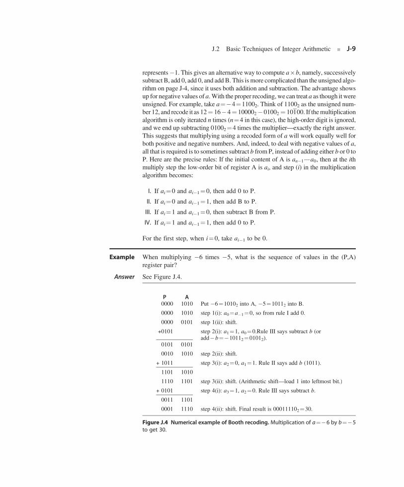
Example
Answer
J.2 Basic Techniques of Integer Arithmetic ■ J-9
represents�1. This gives an alternative way to compute a�b, namely, successivelysubtract B, add 0, add 0, and add B. This is more complicated than the unsigned algo-rithm on page J-4, since it uses both addition and subtraction. The advantage showsup for negative values of a.With the proper recoding, we can treat a as though it wereunsigned. For example, take a¼�4¼11002. Think of 11002 as the unsigned num-ber 12, and recode it as 12¼ 16�4¼ 100002�01002 ¼ 10100. If themultiplicationalgorithm is only iterated n times (n¼4 in this case), the high-order digit is ignored,and we end up subtracting 01002¼4 times the multiplier—exactly the right answer.This suggests that multiplying using a recoded form of a will work equally well forboth positive and negative numbers. And, indeed, to deal with negative values of a,all that is required is to sometimes subtract b from P, instead of adding either b or 0 toP. Here are the precise rules: If the initial content of A is an�1⋯a0, then at the ithmultiply step the low-order bit of register A is ai, and step (i) in the multiplicationalgorithm becomes:
I. If ai¼0 and ai�1¼0, then add 0 to P.
II. If ai¼0 and ai�1¼1, then add B to P.
III. If ai¼1 and ai�1¼0, then subtract B from P.
IV. If ai¼1 and ai�1¼1, then add 0 to P.
For the first step, when i¼0, take ai�1 to be 0.
When multiplying �6 times �5, what is the sequence of values in the (P,A)
register pair?See Figure J.4.
Figure J.4 Numerical example of Booth recoding. Multiplication of a¼�6 by b¼�5to get 30.
J-10 ■ Appendix J Computer Arithmetic
The four prior cases can be restated as saying that in the ith step you should add(ai�1�ai)B to P. With this observation, it is easy to verify that these rules work,because the result of all the additions is
Xn�1
i¼0
b ai�1�aið Þ2i ¼ b �an�12n�1 + an�22
n�2 +… + a12 + a0� �
+ ba�1
Using Equation J.2.3 (page J-8) together with a�1¼0, the right-hand side is seen tobe the value of b�a as a two’s complement number.
The simplest way to implement the rules for Booth recoding is to extend the Aregister one bit to the right so that this new bit will contain ai�1. Unlike the naivemethod of inverting any negative operands, this technique doesn’t require extrasteps or any special casing for negative operands. It has only slightly more controllogic. If the multiplier is being shared with a divider, there will already be the capa-bility for subtracting b, rather than adding it. To summarize, a simple method forhandling two’s complement multiplication is to pay attention to the sign of P whenshifting it right, and to save the most recently shifted-out bit of A to use in decidingwhether to add or subtract b from P.
Booth recoding is usually the best method for designing multiplication hardwarethat operates on signed numbers. For hardware that doesn’t directly implement it,however, performing Booth recoding in software or microcode is usually too slowbecause of the conditional tests and branches. If the hardware supports arithmeticshifts (so that negative b is handled correctly), then the following method can beused. Treat the multiplier a as if it were an unsigned number, and perform the firstn�1multiply steps using the algorithm on page J-4. If a<0 (in which case there willbe a 1 in the low-order bit of the A register at this point), then subtract b from P;otherwise (a�0), neither add nor subtract. In either case, do a final shift (for a totalof n shifts). This works because it amounts to multiplying b by�an�12n�1 +⋯+ a12 + a0, which is the value of an�1⋯a0 as a two’s complementnumber by Equation J.2.3. If the hardware doesn’t support arithmetic shift, thenconverting the operands to be nonnegative is probably the best approach.
Two final remarks: A good way to test a signed-multiply routine is totry �2n�1��2n�1, since this is the only case that produces a 2n�1 bit result.Unlike multiplication, division is usually performed in hardware by convertingthe operands to be nonnegative and then doing an unsigned divide. Because divi-sion is substantially slower (and less frequent) than multiplication, the extra time
used to manipulate the signs has less impact than it does on multiplication.Systems Issues
When designing an instruction set, a number of issues related to integer arithmeticneed to be resolved. Several of them are discussed here.
First, what should be done about integer overflow? This situation is compli-cated by the fact that detecting overflow differs depending on whether the operands
are signed or unsigned integers. Consider signed arithmetic first. There are three
Figure J.5 Summary of howtion that traps if the V bit is
J.2 Basic Techniques of Integer Arithmetic ■ J-11
approaches: Set a bit on overflow, trap on overflow, or do nothing on overflow. Inthe last case, software has to check whether or not an overflow occurred. The mostconvenient solution for the programmer is to have an enable bit. If this bit is turnedon, then overflow causes a trap. If it is turned off, then overflow sets a bit (or, alter-natively, have two different add instructions). The advantage of this approach isthat both trapping and nontrapping operations require only one instruction. Fur-thermore, as we will see in Section J.7, this is analogous to how the IEEEfloating-point standard handles floating-point overflow. Figure J.5 shows howsome common machines treat overflow.
What about unsigned addition? Notice that none of the architectures inFigure J.5 traps on unsigned overflow. The reason for this is that the primaryuse of unsigned arithmetic is in manipulating addresses. It is convenient to be ableto subtract from an unsigned address by adding. For example, when n¼4, we cansubtract 2 from the unsigned address 10¼10102 by adding 14¼11102. Thisgenerates an overflow, but we would not want a trap to be generated.
A second issue concerns multiplication. Should the result of multiplying twon-bit numbers be a 2n-bit result, or should multiplication just return the low-order nbits, signaling overflow if the result doesn’t fit in n bits? An argument in favor of ann-bit result is that in virtually all high-level languages, multiplication is an oper-ation in which arguments are integer variables and the result is an integer variableof the same type. Therefore, compilers won’t generate code that utilizes a double-precision result. An argument in favor of a 2n-bit result is that it can be used by anassembly language routine to substantially speed up multiplication of multiple-precision integers (by about a factor of 3).
A third issue concerns machines that want to execute one instruction every cycle.It is rarely practical to perform amultiplication or division in the same amount of timethat an addition or register-registermove takes. There are three possible approaches tothis problem. The first is to have a single-cyclemultiply-step instruction. This mightdo one step of the Booth algorithm. The second approach is to do integer multipli-
cation in the floating-point unit and have it be part of the floating-point instruction set.various machines handle integer overflow. Both the 8086 and SPARC have an instruc-set, so the cost of trapping on overflow is one extra instruction.
J-12 ■ Appendix J Computer Arithmetic
(This is what DLX does.) The third approach is to have an autonomous unit in theCPUdo themultiplication. In this case, the result either can be guaranteed to be deliv-ered in a fixed number of cycles—and the compiler charged with waiting the properamount of time—or there can be an interlock. The same comments apply to divisionas well. As examples, the original SPARC had a multiply-step instruction but nodivide-step instruction,while theMIPSR3000has an autonomous unit that doesmul-tiplication and division (newer versions of the SPARC architecture added an integermultiply instruction). The designers of the HP Precision Architecture did an espe-cially thorough job of analyzing the frequency of the operands for multiplicationand division, and they based their multiply and divide steps accordingly. (SeeMagenheimer et al. [1988] for details.)
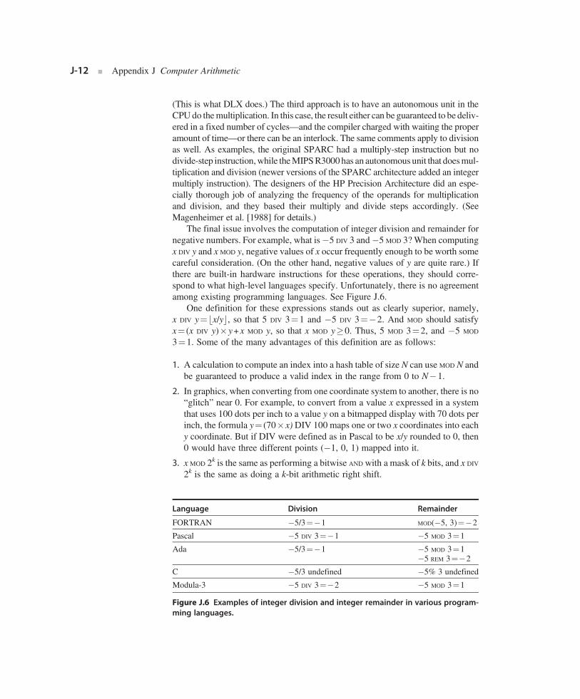
The final issue involves the computation of integer division and remainder fornegative numbers. For example, what is�5 DIV 3 and�5 MOD 3?When computingx DIV y and x MOD y, negative values of x occur frequently enough to be worth somecareful consideration. (On the other hand, negative values of y are quite rare.) Ifthere are built-in hardware instructions for these operations, they should corre-spond to what high-level languages specify. Unfortunately, there is no agreementamong existing programming languages. See Figure J.6.
One definition for these expressions stands out as clearly superior, namely,x DIV y¼bx/yc, so that 5 DIV 3¼1 and �5 DIV 3¼�2. And MOD should satisfyx¼ (x DIV y)�y+x MOD y, so that x MOD y�0. Thus, 5 MOD 3¼2, and �5 MOD
3¼1. Some of the many advantages of this definition are as follows:
1. A calculation to compute an index into a hash table of size N can use MOD N andbe guaranteed to produce a valid index in the range from 0 to N�1.
2. In graphics, when converting from one coordinate system to another, there is no“glitch” near 0. For example, to convert from a value x expressed in a systemthat uses 100 dots per inch to a value y on a bitmapped display with 70 dots perinch, the formula y¼ (70�x) DIV 100 maps one or two x coordinates into eachy coordinate. But if DIV were defined as in Pascal to be x/y rounded to 0, then0 would have three different points (�1, 0, 1) mapped into it.
3. x MOD 2k is the same as performing a bitwise AND with a mask of k bits, and x DIV
2k is the same as doing a k-bit arithmetic right shift.
Figure J.6 Examples of integer division and integer remainder in various program-ming languages.

J.3
J.3 Floating Point ■ J-13
Finally, a potential pitfall worth mentioning concerns multiple-precision addi-tion. Many instruction sets offer a variant of the add instruction that adds threeoperands: two n-bit numbers together with a third single-bit number. This thirdnumber is the carry from the previous addition. Since the multiple-precision num-ber will typically be stored in an array, it is important to be able to increment the
array pointer without destroying the carry bit.Floating Point
Many applications require numbers that aren’t integers. There are a number ofways that nonintegers can be represented. One is to use fixed point; that is, use inte-ger arithmetic and simply imagine the binary point somewhere other than just tothe right of the least-significant digit. Adding two such numbers can be done withan integer add, whereas multiplication requires some extra shifting. Other repre-sentations that have been proposed involve storing the logarithm of a number anddoing multiplication by adding the logarithms, or using a pair of integers (a,b) torepresent the fraction a/b.However, only one noninteger representation has gainedwidespread use, and that is floating point. In this system, a computer word isdivided into two parts, an exponent and a significand. As an example, an exponentof�3 and a significand of 1.5 might represent the number 1.5�2�3¼0.1875. Theadvantages of standardizing a particular representation are obvious. Numericalanalysts can build up high-quality software libraries, computer designers candevelop techniques for implementing high-performance hardware, and hardwarevendors can build standard accelerators. Given the predominance of thefloating-point representation, it appears unlikely that any other representation willcome into widespread use.
The semantics of floating-point instructions are not as clear-cut as the seman-tics of the rest of the instruction set, and in the past the behavior of floating-pointoperations varied considerably from one computer family to the next. The varia-tions involved such things as the number of bits allocated to the exponent andsignificand, the range of exponents, how rounding was carried out, and the actionstaken on exceptional conditions like underflow and overflow. Computer architec-ture books used to dispense advice on how to deal with all these details, butfortunately this is no longer necessary. That’s because the computer industry is rap-idly converging on the format specified by IEEE standard 754-1985 (also an inter-national standard, IEC 559). The advantages of using a standard variant offloating point are similar to those for using floating point over other nonintegerrepresentations.
IEEE arithmetic differs from many previous arithmetics in the following majorways:
1. When rounding a “halfway” result to the nearest floating-point number, it picksthe one that is even.
2. It includes the special values NaN, ∞, and�∞.

J-14 ■ Appendix J Computer Arithmetic
3. It uses denormal numbers to represent the result of computations whose value isless than 1:0�2Emin .
4. It rounds to nearest by default, but it also has three other rounding modes.
5. It has sophisticated facilities for handling exceptions.
To elaborate on (1), note that when operating on two floating-point numbers,the result is usually a number that cannot be exactly represented as anotherfloating-point number. For example, in a floating-point system using base 10and two significant digits, 6.1�0.5¼3.05. This needs to be rounded to two digits.Should it be rounded to 3.0 or 3.1? In the IEEE standard, such halfway cases arerounded to the number whose low-order digit is even. That is, 3.05 rounds to 3.0,not 3.1. The standard actually has four rounding modes. The default is round tonearest, which rounds ties to an even number as just explained. The other modesare round toward 0, round toward+∞, and round toward�∞.
We will elaborate on the other differences in following sections. For further
reading, see IEEE [1985], Cody et al. [1984], and Goldberg [1991].Special Values and Denormals
Probably the most notable feature of the standard is that by default a computationcontinues in the face of exceptional conditions, such as dividing by 0 or taking thesquare root of a negative number. For example, the result of taking the square rootof a negative number is a NaN (Not a Number), a bit pattern that does not representan ordinary number. As an example of how NaNs might be useful, consider thecode for a zero finder that takes a function F as an argument and evaluates F atvarious points to determine a zero for it. If the zero finder accidentally probes out-side the valid values for F, then F may well cause an exception. Writing a zerofinder that deals with this case is highly language and operating-system dependent,because it relies on how the operating system reacts to exceptions and how thisreaction is mapped back into the programming language. In IEEE arithmetic itis easy to write a zero finder that handles this situation and runs on many differentsystems. After each evaluation of F, it simply checks to see whether F has returneda NaN; if so, it knows it has probed outside the domain of F.
In IEEE arithmetic, if the input to an operation is a NaN, the output is NaN(e.g., 3+NaN¼NaN). Because of this rule, writing floating-point subroutines thatcan accept NaN as an argument rarely requires any special case checks. For exam-ple, suppose that arccos is computed in terms of arctan, using the formula
arccosx¼ 2arctanffiffiffiffiffiffiffiffiffiffiffiffiffiffiffiffiffiffiffiffiffiffiffiffiffiffiffiffiffi1� xð Þ= 1 + xð Þp� �
. If arctan handles an argument of NaNproperly, arccos will automatically do so, too. That’s because if x is a NaN,
1 +x, 1�x, (1+x)/(1�x), andffiffiffiffiffiffiffiffiffiffiffiffiffiffiffiffiffiffiffiffiffiffiffiffiffiffiffiffiffi1� xð Þ= 1 + xð Þp
will also be NaNs. No checkingfor NaNs is required.
While the result offfiffiffiffiffiffiffi�1
pis a NaN, the result of 1/0 is not a NaN, but +∞, which
is another special value. The standard defines arithmetic on infinities (there are

Example
Answer
J.3 Floating Point ■ J-15
both +∞ and �∞) using rules such as 1/∞¼0. The formulaarccosx¼ 2arctan
ffiffiffiffiffiffiffiffiffiffiffiffiffiffiffiffiffiffiffiffiffiffiffiffiffiffiffiffiffi1� xð Þ= 1 + xð Þp� �
illustrates how infinity arithmetic can beused. Since arctan x asymptotically approaches π/2 as x approaches∞, it is naturalto define arctan(∞)¼π/2, in which case arccos(�1) will automatically be com-puted correctly as 2 arctan(∞)¼π.
The final kind of special values in the standard are denormal numbers. In manyfloating-point systems, if Emin is the smallest exponent, a number less than 1:0�2Emin cannot be represented, and a floating-point operation that results in a numberless than this is simply flushed to 0. In the IEEE standard, on the other hand, num-bers less than 1:0�2Emin are represented using significands less than 1. This iscalled gradual underflow. Thus, as numbers decrease in magnitude below 2Emin ,they gradually lose their significance and are only represented by 0 when all theirsignificance has been shifted out. For example, in base 10 with four significantfigures, let x¼ 1:234�10Emin . Then, x/10 will be rounded to 0:123�10Emin , havinglost a digit of precision. Similarly x/100 rounds to 0:012�10Emin , and x/1000 to0:001�10Emin , while x/10000 is finally small enough to be rounded to 0. Denor-mals make dealing with small numbers more predictable by maintaining familiarproperties such as x¼y, x�y¼0. For example, in a flush-to-zero system (againin base 10 with four significant digits), if x¼ 1:256�10Emin and y¼ 1:234�10Emin ,then x� y¼ 0:022�10Emin , which flushes to zero. So even though x 6¼y, thecomputed value of x�y¼0. This never happens with gradual underflow. In thisexample, x� y¼ 0:022�10Emin is a denormal number, and so the computation of
x�y is exact.Representation of Floating-Point Numbers
Let us consider how to represent single-precision numbers in IEEE arithmetic.Single-precision numbers are stored in 32 bits: 1 for the sign, 8 for the exponent,and 23 for the fraction. The exponent is a signed number represented using the biasmethod (see the subsection “Signed Numbers,” page J-7) with a bias of 127. Theterm biased exponent refers to the unsigned number contained in bits 1 through 8,and unbiased exponent (or just exponent) means the actual power to which 2 is tobe raised. The fraction represents a number less than 1, but the significand of thefloating-point number is 1 plus the fraction part. In other words, if e is the biasedexponent (value of the exponent field) and f is the value of the fraction field, the
number being represented is 1. f�2e�127.What single-precision number does the following 32-bit word represent?
1 10000001 01000000000000000000000
Considered as an unsigned number, the exponent field is 129, making the value ofthe exponent 129�127¼2. The fraction part is .012¼ .25, making the significand
1.25. Thus, this bit pattern represents the number �1.25�22¼�5.
J-16 ■ Appendix J Computer Arithmetic
The fractional part of a floating-point number (.25 in the example above) mustnot be confused with the significand, which is 1 plus the fractional part. The lead-ing 1 in the significand 1.f does not appear in the representation; that is, the leadingbit is implicit. When performing arithmetic on IEEE format numbers, the fractionpart is usually unpacked, which is to say the implicit 1 is made explicit.
Figure J.7 summarizes the parameters for single (and other) precisions.It shows the exponents for single precision to range from �126 to 127; accord-ingly, the biased exponents range from 1 to 254. The biased exponents of 0 and255 are used to represent special values. This is summarized in Figure J.8. Whenthe biased exponent is 255, a zero fraction field represents infinity, and a nonzerofraction field represents a NaN. Thus, there is an entire family of NaNs. When thebiased exponent and the fraction field are 0, then the number represented is 0.Because of the implicit leading 1, ordinary numbers always have a significandgreater than or equal to 1. Thus, a special convention such as this is required torepresent 0. Denormalized numbers are implemented by having a word with a zeroexponent field represent the number 0:f �2Emin .
The primary reason why the IEEE standard, like most other floating-point for-mats, uses biased exponents is that it means nonnegative numbers are ordered inthe same way as integers. That is, the magnitude of floating-point numbers can becompared using an integer comparator. Another (related) advantage is that 0 is repre-sented by a word of all 0s. The downside of biased exponents is that adding them is
slightly awkward, because it requires that the bias be subtracted from their sum.Figure J.7 Format parameters for the IEEE 754 floating-point standard. The first rowgives the number of bits in the significand. The blanks are unspecified parameters.
Figure J.8 Representation of special values.When the exponent of a number falls out-side the range Emin�e�Emax, then that number has a special interpretation as indicatedin the table.

J.4 Floating-Point Multiplication ■ J-17
J.4
Example
Answer
Floating-Point Multiplication
The simplest floating-point operation is multiplication, so we discuss it first. Abinary floating-point number x is represented as a significand and an exponent,x¼ s�2e. The formula
s1�2e1� �� s2�2e2
� �¼ s1 � s2ð Þ�2e1 + e2
shows that a floating-point multiply algorithm has several parts. The first part mul-tiplies the significands using ordinary integer multiplication. Because floating-point numbers are stored in sign magnitude form, the multiplier need only dealwith unsigned numbers (although we have seen that Booth recoding handlessigned two’s complement numbers painlessly). The second part rounds the result.If the significands are unsigned p-bit numbers (e.g., p¼24 for single precision),then the product can have as many as 2p bits and must be rounded to a p-bit num-ber. The third part computes the new exponent. Because exponents are stored with
a bias, this involves subtracting the bias from the sum of the biased exponents.How does the multiplication of the single-precision numbers
1 1000001 0000… ¼ �1�23
0 1000001 1000… ¼ 1�24
proceed in binary?
When unpacked, the significands are both 1.0, their product is 1.0, and so the resultis of the form:
1 ???????? 000…
To compute the exponent, use the formula:
biased exp e1 + e2ð Þ¼ biased exp e1ð Þ + biased exp e2ð Þ�bias
From Figure J.7, the bias is 127¼011111112, so in two’s complement �127 is100000012. Thus, the biased exponent of the product is
1000001010000011
+ 1000000110000110
Since this is 134 decimal, it represents an exponent of 134�bias¼134�127, as
expected.The interesting part of floating-point multiplication is rounding. Some of thedifferent cases that can occur are illustrated in Figure J.9. Since the cases are similar
in all bases, the figure uses human-friendly base 10, rather than base 2.
Figure J.9 Examples of rounding a multiplication. Using base 10 and p¼3, parts (a)and (b) illustrate that the result of a multiplication can have either 2p�1 or 2p digits;hence, the position where a 1 is added when rounding up (just left of the arrow) can
J-18 ■ Appendix J Computer Arithmetic
In the figure, p¼3, so the final result must be rounded to three significantdigits. The three most-significant digits are in boldface. The fourth most-significant digit (marked with an arrow) is the round digit, denoted by r.
If the round digit is less than 5, then the bold digits represent the rounded result. Ifthe round digit is greater than 5 (as in part (a)), then 1 must be added to the least-significant bold digit. If the round digit is exactly 5 (as in part (b)), then additionaldigits must be examined to decide between truncation or incrementing by 1. It is onlynecessary to know if any digits past 5 are nonzero. In the algorithm below, thiswill berecorded in a sticky bit. Comparing parts (a) and (b) in the figure shows that there aretwo possible positions for the round digit (relative to the least-significant digit of theproduct). Case (c) illustrates that, when adding 1 to the least-significant bold digit,there may be a carry-out. When this happens, the final significand must be 10.0.
There is a straightforward method of handling rounding using the multiplier ofFigure J.2 (page J-4) together with an extra sticky bit. If p is the number of bits inthe significand, then the A, B, and P registers should be p bits wide. Multiply thetwo significands to obtain a 2p-bit product in the (P,A) registers (see Figure J.10).During the multiplication, the first p�2 times a bit is shifted into the A register, ORit into the sticky bit. This will be used in halfway cases. Let s represent the stickybit, g (for guard) the most-significant bit of A, and r (for round) the second most-significant bit of A. There are two cases:
1. The high-order bit of P is 0. Shift P left 1 bit, shifting in the g bit from A. Shift-ing the rest of A is not necessary.
2. The high-order bit of P is 1. Set s :¼ s _ r and r :¼ g, and add 1 to the exponent.
Now if r¼0, P is the correctly rounded product. If r¼1 and s¼1, then P+1 is
vary. Part (c) shows that rounding up can cause a carry-out.
the product (where by P+1 we mean adding 1 to the least-significant bit of P).

Example
Answer
Figure J.10 The two cases of the floating-point multiply algorithm. The top lineshows the contents of the P and A registers after multiplying the significands, withp¼6. In case (1), the leading bit is 0, and so the P register must be shifted. In case(2), the leading bit is 1, no shift is required, but both the exponent and the roundand sticky bits must be adjusted. The sticky bit is the logical OR of the bits marked s.
J.4 Floating-Point Multiplication ■ J-19
If r¼1 and s¼0, we are in a halfway case and round up according to the least-significant bit of P. As an example, apply the decimal version of these rules toFigure J.9(b). After the multiplication, P¼126 and A¼501, with g¼5, r¼0and s¼1. Since the high-order digit of P is nonzero, case (2) applies andr :¼ g, so that r¼5, as the arrow indicates in Figure J.9. Since r¼5, we couldbe in a halfway case, but s¼1 indicates that the result is in fact slightly over1/2, so add 1 to P to obtain the correctly rounded product.
The precise rules for rounding depend on the rounding mode and are given inFigure J.11. Note that P is nonnegative, that is, it contains the magnitude of theresult. A good discussion of more efficient ways to implement rounding is in
Santoro, Bewick, and Horowitz [1989].In binary with p¼4, show how the multiplication algorithm computes the product
�5�10 in each of the four rounding modes.In binary,�5 is�1.0102�22 and 10¼1.0102�23. Applying the integer multipli-cation algorithm to the significands gives 011001002, so P¼01102, A¼01002,g¼0, r¼1, and s¼0. The high-order bit of P is 0, so case (1) applies. Thus, P
becomes 11002, and since the result is negative, Figure J.11 gives:round to�∞ 11012 add 1 since r _ s¼1 / 0¼TRUE
round to+∞ 11002
round to 0 11002
round to nearest 11002 no add since r ^ p0¼1 ^ 0¼FALSE and
ing to�∞, in which c
ase it is �1.1 012�25¼�52.r ^ s¼1 ^ 0¼FALSE
The exponent is 2+3¼5, so the result is�1.1002�25¼�48, except when round-

Figure J.11 Rules for implementing the IEEE roundingmodes. Let S be themagnitudeof the preliminary result. Blanks mean that the pmost-significant bits of S are the actualresult bits. If the condition listed is true, add 1 to the pth most-significant bit of S. Thesymbols r and s represent the round and sticky bits, while p0 is the pth most-significant
J-20 ■ Appendix J Computer Arithmetic
Overflow occurs when the rounded result is too large to be represented. In sin-gle precision, this occurs when the result has an exponent of 128 or higher. If e1 ande2 are the two biased exponents, then 1�ei�254, and the exponent calculatione1+e2�127 gives numbers between 1+1�127 and 254+254�127, or between�125 and 381. This range of numbers can be represented using 9 bits. So one wayto detect overflow is to perform the exponent calculations in a 9-bit adder (seeExercise J.12). Remember that you must check for overflow after rounding—the example in Figure J.9(c) shows that this can make a difference.
Denormals
Checking for underflow is somewhat more complex because of denormals. In sin-gle precision, if the result has an exponent less than�126, that does not necessarilyindicate underflow, because the result might be a denormal number. For example,the product of (1�2�64) with (1�2�65) is 1�2�129, and �129 is below the legalexponent limit. But this result is a valid denormal number, namely, 0.125�2�126.In general, when the unbiased exponent of a product dips below �126, the result-ing product must be shifted right and the exponent incremented until the exponentreaches �126. If this process causes the entire significand to be shifted out, thenunderflow has occurred. The precise definition of underflow is somewhat subtle—see Section J.7 for details.
When one of the operands of a multiplication is denormal, its significand willhave leading zeros, and so the product of the significands will also have leadingzeros. If the exponent of the product is less than�126, then the result is denormal,so right-shift and increment the exponent as before. If the exponent is greater than�126, the result may be a normalized number. In this case, left-shift the product(while decrementing the exponent) until either it becomes normalized or theexponent drops to �126.
Denormal numbers present a major stumbling block to implementingfloating-point multiplication, because they require performing a variableshift in the multiplier, which wouldn’t otherwise be needed. Thus, high-
bit of S.
performance, floating-point multipliers often do not handle denormalized

J.5
J.5 Floating-Point Addition ■ J-21
numbers, but instead trap, letting software handle them. A few practical codesfrequently underflow, even when working properly, and these programs willrun quite a bit slower on systems that require denormals to be processed bya trap handler.
So far we haven’t mentioned how to deal with operands of zero. This can behandled by either testing both operands before beginning the multiplication or test-ing the product afterward. If you test afterward, be sure to handle the case 0�∞properly: This results in NaN, not 0. Once you detect that the result is 0, set thebiased exponent to 0. Don’t forget about the sign. The sign of a product is theXOR of the signs of the operands, even when the result is 0.
Precision of Multiplication
In the discussion of integer multiplication, we mentioned that designers mustdecide whether to deliver the low-order word of the product or the entire prod-uct. A similar issue arises in floating-point multiplication, where the exactproduct can be rounded to the precision of the operands or to the next higherprecision. In the case of integer multiplication, none of the standard high-levellanguages contains a construct that would generate a “single times single getsdouble” instruction. The situation is different for floating point. Many lan-guages allow assigning the product of two single-precision variables to adouble-precision one, and the construction can also be exploited by numericalalgorithms. The best-known case is using iterative refinement to solve linear
systems of equations.Floating-Point Addition
Typically, a floating-point operation takes two inputs with p bits of precision andreturns a p-bit result. The ideal algorithm would compute this by first performingthe operation exactly, and then rounding the result to p bits (using the currentrounding mode). The multiplication algorithm presented in the previous sectionfollows this strategy. Even though hardware implementing IEEE arithmetic mustreturn the same result as the ideal algorithm, it doesn’t need to actually perform theideal algorithm. For addition, in fact, there are better ways to proceed. To see this,consider some examples.
First, the sum of the binary 6-bit numbers 1.100112 and 1.100012�2�5: Whenthe summands are shifted so they have the same exponent, this is
1:10011+ :0000110001
Using a 6-bit adder (and discarding the low-order bits of the second addend) gives
1:10011+ :00001
+ 1:10100
J-22 ■ Appendix J Computer Arithmetic
The first discarded bit is 1. This isn’t enough to decide whether to round up. Therest of the discarded bits, 0001, need to be examined. Or, actually, we just need torecord whether any of these bits are nonzero, storing this fact in a sticky bit just asin the multiplication algorithm. So, for adding two p-bit numbers, a p-bit adder issufficient, as long as the first discarded bit (round) and the OR of the rest of thebits (sticky) are kept. Then Figure J.11 can be used to determine if a roundup isnecessary, just as with multiplication. In the example above, sticky is 1, so aroundup is necessary. The final sum is 1.101012.
Here’s another example:
1:11011+ :0101001
A 6-bit adder gives:
1:11011+ :01010+ 10:00101
Because of the carry-out on the left, the round bit isn’t the first discarded bit; rather,it is the low-order bit of the sum (1). The discarded bits, 01, are OR’ed together tomake sticky. Because round and sticky are both 1, the high-order 6 bits of the sum,10.00102, must be rounded up for the final answer of 10.00112.
Next, consider subtraction and the following example:
1:00000� :00000101111
The simplest way of computing this is to convert� .000001011112 to its two’scomplement form, so the difference becomes a sum:
1:00000+ 1:11111010001
Computing this sum in a 6-bit adder gives:
1:00000+ 1:11111
0:11111
Because the top bits canceled, the first discarded bit (the guard bit) is needed to fill inthe least-significant bit of the sum, which becomes 0.1111102, and the second dis-carded bit becomes the round bit. This is analogous to case (1) in the multiplicationalgorithm (see page J-19). The round bit of 1 isn’t enough to decide whether to roundup. Instead, we need to OR all the remaining bits (0001) into a sticky bit. In this case,sticky is1, so the final resultmustbe roundedup to0.111111.Thisexample shows thatif subtraction causes themost-significant bit to cancel, then one guard bit is needed. Itis natural to ask whether two guard bits are needed for the case when the two most-significant bits cancel. The answer is no, because if x and y are so close that the top
two bits of x�y cancel, then x�y will be exact, so guard bits aren’t needed at all.
J.5 Floating-Point Addition ■ J-23
To summarize, addition is more complex than multiplication because, depend-ing on the signs of the operands, it may actually be a subtraction. If it is an addition,there can be carry-out on the left, as in the second example. If it is subtraction, therecan be cancellation, as in the third example. In each case, the position of the roundbit is different. However, we don’t need to compute the exact sum and then round.We can infer it from the sum of the high-order p bits together with the round andsticky bits.
The rest of this section is devoted to a detailed discussion of the floatingpointaddition algorithm. Let a1 and a2 be the two numbers to be added. The notations eiand si are used for the exponent and significand of the addends ai. This means thatthe floating-point inputs have been unpacked and that si has an explicit leading bit.To add a1 and a2, perform these eight steps:
1. If e1<e2, swap the operands. This ensures that the difference of the exponentssatisfies d¼e1�e2�0. Tentatively set the exponent of the result to e1.
2. If the signs of a1 and a2 differ, replace s2 by its two’s complement.
3. Place s2 in a p-bit register and shift it d¼e1�e2 places to the right (shifting in1’s if s2 was complemented in the previous step). From the bits shifted out, set gto the most-significant bit, set r to the next most-significant bit, and set sticky tothe OR of the rest.
4. Compute a preliminary significand S¼ s1+ s2 by adding s1 to the p-bit registercontaining s2. If the signs of a1 and a2 are different, the most-significant bit of Sis 1, and there was no carry-out, then S is negative. Replace S with its two’scomplement. This can only happen when d¼0.
5. Shift S as follows. If the signs of a1 and a2 are the same and there was a carryoutin step 4, shift S right by one, filling in the high-order position with 1 (the carry-out). Otherwise, shift it left until it is normalized. When left-shifting, on the firstshift fill in the low-order position with the g bit. After that, shift in zeros. Adjustthe exponent of the result accordingly.
6. Adjust r and s. If S was shifted right in step 5, set r :¼ low-order bit of S beforeshifting and s :¼ g OR r OR s. If there was no shift, set r :¼ g, s :¼ r OR s. Ifthere was a single left shift, don’t change r and s. If there were two or more leftshifts, r :¼ 0, s :¼ 0. (In the last case, two or more shifts can only happen whena1 and a2 have opposite signs and the same exponent, in which case the com-putation s1+ s2 in step 4 will be exact.)
7. Round S using Figure J.11; namely, if a table entry is nonempty, add 1 to thelow-order bit of S. If rounding causes carry-out, shift S right and adjust the expo-nent. This is the significand of the result.
8. Compute the sign of the result. If a1 and a2 have the same sign, this is the sign ofthe result. If a1 and a2 have different signs, then the sign of the result depends onwhich of a1 or a2 is negative, whether there was a swap in step 1, and whether S
was replaced by its two’s complement in step 4. See Figure J.12.
Answer
Answer
Figure J.12 Rules for computing the sign of a sum when the addends havedifferent signs. The swap column refers to swapping the operands in step 1, while thecompl column refers to performing a two’s complement in step 4. Blanks are “don’t care.”
J-24 ■ Appendix J Computer Arithmetic
�2 0
Example Use the algorithm to compute the sum (�1.0012�2 )+ (�1.1112�2 ).s1¼1.001, e1¼�2, s2¼1.111, e2¼0
1. e1<e2, so swap. d¼2. Tentative exp¼0.
2. Signs of both operands negative, don’t negate s2.
3. Shift s2 (1.001 after swap) right by 2, giving s2¼ .010, g¼0, r¼1, s¼0.
4.1:111
+ :010
1ð Þ0:001 S¼ 0:001, with a carry�out:
5. Carry-out, so shift S right, S¼1.000, exp¼exp+1, so exp¼1.
6. r¼ low-order bit of sum¼1, s¼g _ r _ s¼0 _ 1 _ 0¼1.
7. r AND s¼TRUE, so Figure J.11 says round up, S¼S+1 or S¼1.001.
8. Both signs negative, so sign of result is negative. Final answer:
�S�2exp¼1.0012�21.Example
Use the algorithm to compute the sum (�1.0102)+1.1002.s1¼1.010, e1¼0, s2¼1.100, e2¼0
1. No swap, d¼0, tentative exp¼0.
2. Signs differ, replace s2 with 0.100.
3. d¼0, so no shift. r¼g¼ s¼0.
4.1:010
+ 0:100
1:110 Signs are different, most-significant bit is 1, no carry-out, so
must two’s complement sum, giving S¼ 0:010:
J.5 Floating-Point Addition ■ J-25
5. Shift left twice, so S¼1.000, exp¼exp�2, or exp¼�2.
6. Two left shifts, so r¼g¼ s¼0.
7. No addition required for rounding.
8. Answer is sign�S�2exp or sign�1.000�2�2. Get sign from Figure J.12.Since complement but no swap and sign(a1) is�, the sign of the sum is +. Thus,
the answer¼1.0002�2�2.Speeding Up Addition
Let’s estimate how long it takes to perform the algorithm above. Step 2 may requirean addition, step 4 requires one or two additions, and step 7 may require an addi-tion. If it takes T time units to perform a p-bit add (where p¼24 for single preci-sion, 53 for double), then it appears the algorithm will take at least 4 T time units.But that is too pessimistic. If step 4 requires two adds, then a1 and a2 have the sameexponent and different signs, but in that case the difference is exact, so no roundupis required in step 7. Thus, only three additions will ever occur. Similarly,it appears that a variable shift may be required both in step 3 and step 5. But ifje1�e2j�1, then step 3 requires a right shift of at most one place, so only step5 needs a variable shift. And, if je1�e2j>1, then step 3 needs a variable shift,but step 5 will require a left shift of at most one place. So only a single variableshift will be performed. Still, the algorithm requires three sequential adds, which,in the case of a 53-bit double-precision significand, can be rather time consuming.
Anumber of techniques can speed up addition.One is to use pipelining. The “Put-ting It All Together” section gives examples of how some commercial chips pipelineaddition. Another method (used on the Intel 860 [Kohn and Fu 1989]) is to performtwo additions in parallel. We now explain how this reduces the latency from 3T to T.
There are three cases to consider. First, suppose that both operands have thesame sign. We want to combine the addition operations from steps 4 and 7. Theposition of the high-order bit of the sum is not known ahead of time, becausethe addition in step 4 may or may not cause a carry-out. Both possibilities areaccounted for by having two adders. The first adder assumes the add in step 4 willnot result in a carry-out. Thus, the values of r and s can be computed before the addis actually done. If r and s indicate that a roundup is necessary, the first adder willcompute S¼ s1+ s2+1, where the notation +1 means adding 1 at the position of theleast-significant bit of s1. This can be done with a regular adder by setting the low-order carry-in bit to 1. If r and s indicate no roundup, the adder computes S¼ s1+ s2as usual. One extra detail: When r¼1, s¼0, you will also need to know the low-order bit of the sum, which can also be computed in advance very quickly. Thesecond adder covers the possibility that there will be carry-out. The values of rand s and the position where the roundup 1 is added are different from above,but again they can be quickly computed in advance. It is not known whether therewill be a carry-out until after the add is actually done, but that doesn’t matter. By
doing both adds in parallel, one adder is guaranteed to reduce the correct answer.
J-26 ■ Appendix J Computer Arithmetic
The next case is when a1 and a2 have opposite signs but the same exponent.The sum a1+a2 is exact in this case (no roundup is necessary) but the sign isn’tknown until the add is completed. So don’t compute the two’s complement (whichrequires an add) in step 2, but instead compute s1 + s2 + 1 and s1 + s2 + 1 in parallel.The first sum has the result of simultaneously complementing s1 and computing thesum, resulting in s2� s1. The second sum computes s1� s2. One of these will benonnegative and hence the correct final answer. Once again, all the additionsare done in one step using two adders operating in parallel.
The last case, when a1 and a2 have opposite signs and different exponents, ismore complex. If je1�e2j>1, the location of the leading bit of the difference is inone of two locations, so there are two cases just as in addition. When je1�e2j¼1,cancellation is possible and the leading bit could be almost anywhere. However,only if the leading bit of the difference is in the same position as the leading bit of s1could a roundup be necessary. So one adder assumes a roundup, and the otherassumes no roundup. Thus, the addition of step 4 and the rounding of step 7can be combined. However, there is still the problem of the addition in step 2!
To eliminate this addition, consider the following diagram of step 4:
j__ __ p __ __js1 1:xxxxxxxs2� 1yyzzzzz
If the bits marked z are all 0, then the high-order p bits of S¼ s1� s2 can be com-puted as s1 + s2 + 1. If at least one of the z bits is 1, use s1 + s2. So s1� s2 can becomputed with one addition. However, we still don’t know g and r for the two’scomplement of s2, which are needed for rounding in step 7.
To compute s1� s2 and get the proper g and r bits, combine steps 2 and 4 asfollows. Don’t complement s2 in step 2. Extend the adder used for computing S twobits to the right (call the extended sum S0). If the preliminary sticky bit (computedin step 3) is 1, compute S0 ¼ s01 + s
02, where s1
0 has two 0 bits tacked onto the right,and s20 has preliminary g and r appended. If the sticky bit is 0, compute s01 + s
02 + 1.
Now the two low-order bits of S0 have the correct values of g and r (the stickybit was already computed properly in step 3). Finally, this modification can becombined with the modification that combines the addition from steps 4 and 7to provide the final result in time T, the time for one addition.
A fewmore details need to be considered, as discussed in Santoro, Bewick, andHorowitz [1989] and Exercise J.17. Although the Santoro paper is aimed at mul-tiplication, much of the discussion applies to addition as well. Also relevant isExercise J.19, which contains an alternative method for adding signed magnitudenumbers.
Denormalized Numbers
Unlike multiplication, for addition very little changes in the preceding descriptionif one of the inputs is a denormal number. There must be a test to see if the exponent
field is 0. If it is, then when unpacking the significand there will not be a leading 1.
J.6
J.6 Division and Remainder ■ J-27
By setting the biased exponent to 1 when unpacking a denormal, the algorithmworks unchanged.
To deal with denormalized outputs, step 5 must be modified slightly. Shift Suntil it is normalized, or until the exponent becomes Emin (that is, the biased expo-nent becomes 1). If the exponent is Emin and, after rounding, the high-order bit of Sis 1, then the result is a normalized number and should be packed in the usual way,by omitting the 1. If, on the other hand, the high-order bit is 0, the result is denor-mal. When the result is unpacked, the exponent field must be set to 0. Section J.7discusses the exact rules for detecting underflow.
Incidentally, detecting overflow is very easy. It can only happen if step 5involves a shift right and the biased exponent at that point is bumped up to 255
in single precision (or 2047 for double precision), or if this occurs after rounding.Division and Remainder
In this section, we’ll discuss floating-point division and remainder.
Iterative Division
We earlier discussed an algorithm for integer division. Converting it into a floating-point division algorithm is similar to converting the integer multiplication algo-rithm into floating point. The formula
s1�2e1ð Þ= s2�2e2ð Þ¼ s1=s2ð Þ�2e1�e2
shows that if the divider computes s1/s2, then the final answer will be this quotientmultiplied by 2e1�e2 . Referring to Figure J.2(b) (page J-4), the alignment of oper-ands is slightly different from integer division. Load s2 into B and s1 into P. The Aregister is not needed to hold the operands. Then the integer algorithm for divi-sion (with the one small change of skipping the very first left shift) can be used,and the result will be of the form q0 � q1⋯. To round, simply compute two addi-tional quotient bits (guard and round) and use the remainder as the sticky bit. Theguard digit is necessary because the first quotient bit might be 0. However, sincethe numerator and denominator are both normalized, it is not possible for the twomost-significant quotient bits to be 0. This algorithm produces one quotient bit ineach step.
A different approach to division converges to the quotient at a quadraticrather than a linear rate. An actual machine that uses this algorithm will be dis-cussed in Section J.10. First, we will describe the two main iterative algorithms,and then we will discuss the pros and cons of iteration when compared with thedirect algorithms. A general technique for constructing iterative algorithms,called Newton’s iteration, is shown in Figure J.13. First, cast the problem inthe form of finding the zero of a function. Then, starting from a guess for the zero,
approximate the function by its tangent at that guess and form a new guess based
J:6:1
J:6:2
xx
i+1x
i
f(x)
f(xi)
Figure J.13 Newton’s iteration for zero finding. If xi is an estimate for a zero of f, thenxi +1 is a better estimate. To compute xi+1, find the intersection of the x-axis with thetangent line to f at f(xi).
J-28 ■ Appendix J Computer Arithmetic
on where the tangent has a zero. If xi is a guess at a zero, then the tangent line hasthe equation:
y� f xið Þ¼ f 0 xið Þ x� xið ÞThis equation has a zero at
x¼ xi+ 1 ¼ xi� f xið Þf 0 xið Þ
To recast division as finding the zero of a function, consider f(x)¼x�1�b. Since thezero of this function is at 1/b, applying Newton’s iteration to it will give an iterativemethod of computing 1/b from b. Using f 0(x)¼�1/x2, Equation J.6.1 becomes:
xi+ 1 ¼ xi�1=xi�b
�1=x2i¼ xi + xi� x2i b¼ xi 2� xibð Þ
Thus, we could implement computation of a/b using the following method:
1. Scale b to lie in the range 1�b<2 and get an approximate value of 1/b (call itx0) using a table lookup.
2. Iterate xi+1¼xi(2�xib) until reaching an xn that is accurate enough.
3. Compute axn and reverse the scaling done in step 1.
Here are some more details. Howmany times will step 2 have to be iterated? Tosay that xi is accurate to p bits means that j(xi�1/b)/(1/b)j¼2�p, and a simple alge-braic manipulation shows that when this is so, then (xi+1�1/b)/(1/b)¼2�2p. Thus,the number of correct bits doubles at each step. Newton’s iteration is self-correct-ing in the sense that making an error in xi doesn’t really matter. That is, it treats xi asa guess at 1/b and returns xi+1 as an improvement on it (roughly doubling the
digits). One thing that would cause xi to be in error is rounding error. More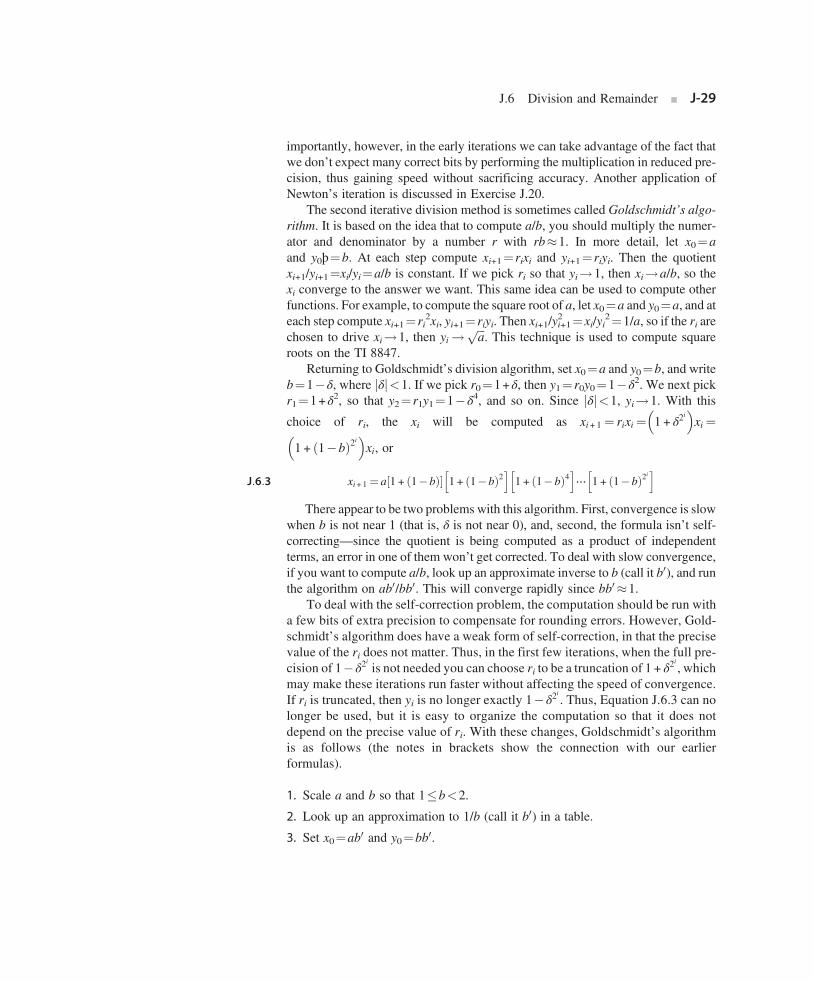
J:6:3
J.6 Division and Remainder ■ J-29
importantly, however, in the early iterations we can take advantage of the fact thatwe don’t expect many correct bits by performing the multiplication in reduced pre-cision, thus gaining speed without sacrificing accuracy. Another application ofNewton’s iteration is discussed in Exercise J.20.
The second iterative division method is sometimes called Goldschmidt’s algo-rithm. It is based on the idea that to compute a/b, you should multiply the numer-ator and denominator by a number r with rb�1. In more detail, let x0¼aand y0þ¼b. At each step compute xi+1¼ rixi and yi+1¼ riyi. Then the quotientxi+1/yi+1¼xi/yi¼a/b is constant. If we pick ri so that yi!1, then xi!a/b, so thexi converge to the answer we want. This same idea can be used to compute otherfunctions. For example, to compute the square root of a, let x0¼a and y0¼a, and ateach step compute xi+1¼ ri
2xi, yi+1¼ riyi. Then xi+1/yi+12 ¼xi/yi
2¼1/a, so if the ri arechosen to drive xi!1, then yi !
ffiffiffia
p. This technique is used to compute square
roots on the TI 8847.Returning to Goldschmidt’s division algorithm, set x0¼a and y0¼b, and write
b¼1�δ, where jδj<1. If we pick r0¼1+δ, then y1¼ r0y0¼1�δ2. We next pickr1¼1+δ2, so that y2¼ r1y1¼1�δ4, and so on. Since jδj<1, yi!1. With this
choice of ri, the xi will be computed as xi + 1 ¼ rixi ¼ 1 + δ2i
� �xi ¼
1 + 1�bð Þ2i� �
xi, or
xi+ 1 ¼ a 1 + 1�bð Þ½ 1 + 1�bð Þ2h i
1 + 1�bð Þ4h i
⋯ 1 + 1�bð Þ2ih i
There appear to be two problems with this algorithm. First, convergence is slowwhen b is not near 1 (that is, δ is not near 0), and, second, the formula isn’t self-correcting—since the quotient is being computed as a product of independentterms, an error in one of them won’t get corrected. To deal with slow convergence,if you want to compute a/b, look up an approximate inverse to b (call it b0), and runthe algorithm on ab0/bb0. This will converge rapidly since bb0 �1.
To deal with the self-correction problem, the computation should be run witha few bits of extra precision to compensate for rounding errors. However, Gold-schmidt’s algorithm does have a weak form of self-correction, in that the precisevalue of the ri does not matter. Thus, in the first few iterations, when the full pre-cision of 1�δ2
iis not needed you can choose ri to be a truncation of 1 + δ
2i , whichmay make these iterations run faster without affecting the speed of convergence.If ri is truncated, then yi is no longer exactly 1�δ2
i. Thus, Equation J.6.3 can no
longer be used, but it is easy to organize the computation so that it does notdepend on the precise value of ri. With these changes, Goldschmidt’s algorithmis as follows (the notes in brackets show the connection with our earlierformulas).
1. Scale a and b so that 1�b<2.
2. Look up an approximation to 1/b (call it b0) in a table.
3. Set x0¼ab0 and y0¼bb0.

J-30 ■ Appendix J Computer Arithmetic
4. Iterate until xi is close enough to a/b:
Loop
r� 2� y if yi ¼ 1 + δi, then r� 1�δi½ y¼ y� r yi+ 1 ¼ yi� r� 1�δi
2� �
xi +1 ¼ xi� r xi +1 ¼ xi� r½ End loop
The two iteration methods are related. Suppose in Newton’s method that weunroll the iteration and compute each term xi+1 directly in terms of b, instead ofrecursively in terms of xi. By carrying out this calculation (see Exercise J.22),we discover that
xi + 1 ¼ x0 2� x0bð Þ 1 + x0b�1ð Þ2� i
1 + x0b�1ð Þ4h i
⋯ 1 + x0b�1ð Þ2ih ih
This formula is very similar to Equation J.6.3. In fact, they are identical if a and b inJ.6.3 are replaced with ax0, bx0, and a¼1. Thus, if the iterations were done to infi-nite precision, the two methods would yield exactly the same sequence xi.
The advantage of iteration is that it doesn’t require special divide hardware.Instead, it can use the multiplier (which, however, requires extra control). Further,on each step, it delivers twice as many digits as in the previous step—unlike ordi-nary division, which produces a fixed number of digits at every step.
There are two disadvantages with inverting by iteration. The first is that theIEEE standard requires division to be correctly rounded, but iteration only deliversa result that is close to the correctly rounded answer. In the case of Newton’s iter-ation, which computes 1/b instead of a/b directly, there is an additional problem.Even if 1/bwere correctly rounded, there is no guarantee that a/bwill be. An exam-ple in decimal with p¼2 is a¼13, b¼51. Then a/b¼ .2549…, which rounds to.25. But 1/b¼ .0196…, which rounds to .020, and then a� .020¼ .26, which is offby 1. The second disadvantage is that iteration does not give a remainder. This isespecially troublesome if the floating-point divide hardware is being used toperform integer division, since a remainder operation is present in almost everyhigh-level language.
Traditional folklore has held that the way to get a correctly rounded result fromiteration is to compute 1/b to slightly more than 2p bits, compute a/b to slightlymore than 2p bits, and then round to p bits. However, there is a faster way, whichapparently was first implemented on the TI 8847. In this method, a/b is computedto about 6 extra bits of precision, giving a preliminary quotient q. By comparing qbwith a (again with only 6 extra bits), it is possible to quickly decide whether qis correctly rounded or whether it needs to be bumped up or down by 1 in theleast-significant place. This algorithm is explored further in Exercise J.21.
One factor to take into account when deciding on division algorithms is the rel-ative speed of division and multiplication. Since division is more complex than mul-tiplication, it will run more slowly. A common rule of thumb is that division
algorithms should try to achieve a speed that is about one-third that of multiplication.
J.6 Division and Remainder ■ J-31
One argument in favor of this rule is that there are real programs (such as some ver-sions of spice) where the ratio of division to multiplication is 1:3. Another placewhere a factor of 3 arises is in the standard iterative method for computing squareroot. This method involves one division per iteration, but it can be replaced by one
using three multiplications. This is discussed in Exercise J.20.Floating-Point Remainder
For nonnegative integers, integer division and remainder satisfy:
a¼ a DIV bð Þb + a REM b, 0� a REM b< b
A floating-point remainder x REM y can be similarly defined as x¼ INT(x/y)y+x REM
y. How should x/y be converted to an integer? The IEEE remainder function usesthe round-to-even rule. That is, pick n¼ INT (x/y) so that jx/y�nj�1/2. If two dif-ferent n satisfy this relation, pick the even one. Then REM is defined to be x�yn.Unlike integers where 0�a REM b<b, for floating-point numbers jx REM yj�y/2.Although this defines REM precisely, it is not a practical operational definition,because n can be huge. In single precision, n could be as large as 2127/2�126¼2253�1076.
There is a natural way to compute REM if a direct division algorithm is used.Proceed as if you were computing x/y. If x¼ s12e1 and y¼ s22e2 and the divideris as in Figure J.2(b) (page J-4), then load s1 into P and s2 into B. After e1�e2division steps, the P register will hold a number r of the form x�yn satisfying0� r<y. Since the IEEE remainder satisfies jREMj�y/2, REM is equal to either ror r�y. It is only necessary to keep track of the last quotient bit produced, whichis needed to resolve halfway cases. Unfortunately, e1�e2 can be a lot of steps, andfloating-point units typically have a maximum amount of time they are allowed tospend on one instruction. Thus, it is usually not possible to implement REM directly.None of the chips discussed in Section J.10 implements REM, but they could byproviding a remainder-step instruction—this is what is done on the Intel 8087 fam-ily. A remainder step takes as arguments two numbers x and y, and performs dividesteps until either the remainder is in P or n steps have been performed, where n is asmall number, such as the number of steps required for division in the highest-supported precision. Then REM can be implemented as a software routine that callsthe REM step instruction b(e1�e2)/nc times, initially using x as the numerator butthen replacing it with the remainder from the previous REM step.
REM can be used for computing trigonometric functions. To simplify things,imagine that we are working in base 10 with five significant figures, and considercomputing sin x. Suppose that x¼7. Then we can reduce by π¼3.1416 and com-pute sin(7)¼ sin(7�2�3.1416)¼ sin(0.7168) instead. But, suppose we want tocompute sin(2.0�105). Then 2�105/3.1416¼63661.8, which in our five-placesystem comes out to be 63662. Since multiplying 3.1416 times 63662 gives200000.5392, which rounds to 2.0000�105, argument reduction reduces
2�105 to 0, which is not even close to being correct. The problem is that our
J.7
J-32 ■ Appendix J Computer Arithmetic
five-place system does not have the precision to do correct argument reduction.Suppose we had the REM operator. Then we could compute 2�105 REM 3.1416and get� .53920. However, this is still not correct because we used 3.1416, whichis an approximation for π. The value of 2�105 REM π is� .071513.
Traditionally, there have been two approaches to computing periodic functionswith large arguments. The first is to return an error for their value when x is large.The second is to store π to a very large number of places and do exact argumentreduction. The REM operator is not much help in either of these situations. There is athird approach that has been used in some math libraries, such as the BerkeleyUNIX 4.3bsd release. In these libraries, π is computed to the nearest floating-pointnumber. Let’s call this machine π, and denote it by π0. Then, when computing sin x,reduce x using x REM π0. As we saw in the above example, x REM π0 is quite differentfrom x REM π when x is large, so that computing sin x as sin(x REM π0) will not givethe exact value of sin x. However, computing trigonometric functions in this fash-ion has the property that all familiar identities (such as sin2x+cos2x¼1) are true towithin a few rounding errors. Thus, using REM together with machine π provides asimple method of computing trigonometric functions that is accurate for smallarguments and still may be useful for large arguments.
When REM is used for argument reduction, it is very handy if it also returns thelow-order bits of n (where x REM y¼x�ny). This is because a practical implemen-tation of trigonometric functions will reduce by something smaller than 2π.For example, it might use π/2, exploiting identities such as sin(x�π/2)¼�cosx, sin(x�π)¼�sin x. Then the low bits of n are needed to choose the correct
identity.More on Floating-Point Arithmetic
Before leaving the subject of floating-point arithmetic, we present a few additionaltopics.
Fused Multiply-Add
Probably the most common use of floating-point units is performing matrixoperations, and the most frequent matrix operation is multiplying a matrix timesa matrix (or vector), which boils down to computing an inner product,x1 �y1+x2 �y2+…+xn �yn. Computing this requires a series of multiply-addcombinations.
Motivated by this, the IBM RS/6000 introduced a single instruction thatcomputes ab+c, the fused multiply-add. Although this requires being able to readthree operands in a single instruction, it has the potential for improving the perfor-mance of computing inner products.
The fused multiply-add computes ab+c exactly and then rounds. Althoughrounding only once increases the accuracy of inner products somewhat, that is
not its primary motivation. There are two main advantages of rounding once. First,
J.7 More on Floating-Point Arithmetic ■ J-33
as we saw in the previous sections, rounding is expensive to implement because itmay require an addition. By rounding only once, an addition operation has beeneliminated. Second, the extra accuracy of fused multiply-add can be used to com-pute correctly rounded division and square root when these are not availabledirectly in hardware. Fused multiply-add can also be used to implement efficientfloating-point multiple-precision packages.
The implementation of correctly rounded division using fused multiply-addhas many details, but the main idea is simple. Consider again the example fromSection J.6 (page J-30), which was computing a/b with a¼13, b¼51. Then 1/brounds to b0 ¼ .020, and ab0 rounds to q0 ¼ .26, which is not the correctly roundedquotient. Applying fused multiply-add twice will correctly adjust the result, via theformulas
r¼ a�bq0
q00 ¼ q0 + rb0
Computing to two-digit accuracy, bq0 ¼51� .26 rounds to 13, and so r¼a�bq0
would be 0, giving no adjustment. But using fused multiply-add givesr¼a�bq0 ¼13� (51� .26)¼� .26, and then q00 ¼q0 + rb0 ¼ .26� .0052¼ .2548,which rounds to the correct quotient, .25. More details can be found in the papers
by Montoye, Hokenek, and Runyon [1990] and Markstein [1990].Precisions
The standard specifies four precisions: single, single extended, double, and doubleextended. The properties of these precisions are summarized in Figure J.7 (page J-16). Implementations are not required to have all four precisions, but are encour-aged to support either the combination of single and single extended or all of sin-gle, double, and double extended. Because of the widespread use of doubleprecision in scientific computing, double precision is almost always implemented.Thus, the computer designer usually only has to decide whether to support doubleextended and, if so, how many bits it should have.
The Motorola 68882 and Intel 387 coprocessors implement extended precisionusing the smallest allowable size of 80 bits (64 bits of significand). However, manyof the more recently designed, high-performance floating-point chips do not imple-ment 80-bit extended precision. One reason is that the 80-bit width of extendedprecision is awkward for 64-bit buses and registers. Some new architectures, suchas SPARC V8 and PA-RISC, specify a 128-bit extended (or quad) precision. Theyhave established a de facto convention for quad that has 15 bits of exponent and113 bits of significand.
Although most high-level languages do not provide access to extended preci-sion, it is very useful to writers of mathematical software. As an example, considerwriting a library routine to compute the length of a vector (x,y) in the plane, namely,ffiffiffiffiffiffiffiffiffiffiffiffiffi
x2 + y2p
. If x is larger than 2Emax=2, then computing this in the obvious way will
overflow. This means that either the allowable exponent range for this subroutine
J-34 ■ Appendix J Computer Arithmetic
will be cut in half or a more complex algorithm using scaling will have to beemployed. But, if extended precision is available, then the simple algorithm willwork. Computing the length of a vector is a simple task, and it is not difficult tocome up with an algorithm that doesn’t overflow. However, there are more com-plex problems for which extended precision means the difference between asimple, fast algorithm and a much more complex one. One of the best examplesof this is binary-to-decimal conversion. An efficient algorithm for binary-to-decimal conversion that makes essential use of extended precision is very readablypresented in Coonen [1984]. This algorithm is also briefly sketched in Goldberg[1991]. Computing accurate values for transcendental functions is another exampleof a problem that is made much easier if extended precision is present.
One very important fact about precision concerns double rounding. To illus-trate in decimals, suppose that we want to compute 1.9�0.66 and that singleprecision is two digits, while extended precision is three digits. The exact resultof the product is 1.254. Rounded to extended precision, the result is 1.25. Whenfurther rounded to single precision, we get 1.2. However, the result of 1.9�0.66correctly rounded to single precision is 1.3. Thus, rounding twice may not pro-duce the same result as rounding once. Suppose you want to build hardware thatonly does double-precision arithmetic. Can you simulate single precision bycomputing first in double precision and then rounding to single? The aboveexample suggests that you can’t. However, double rounding is not alwaysdangerous. In fact, the following rule is true (this is not easy to prove, butsee Exercise J.25).
If x and y have p-bit significands, and x+y is computed exactly and then roundedto q places, a second rounding to p places will not change the answer if q�2p+2.This is true not only for addition, but also for multiplication, division, and squareroot.
In our example above, q¼3 and p¼2, so q Š 2p+2 is not true. On the otherhand, for IEEE arithmetic, double precision has q¼53 and p¼24, so q¼53 Š2p +2¼50. Thus, single precision can be implemented by computing in doubleprecision—that is, computing the answer exactly and then rounding to double—and then rounding to single precision.
Exceptions
The IEEE standard defines five exceptions: underflow, overflow, divide by zero,inexact, and invalid. By default, when these exceptions occur, they merely set aflag and the computation continues. The flags are sticky, meaning that once set theyremain set until explicitly cleared. The standard strongly encourages implementa-tions to provide a trap-enable bit for each exception. When an exception with anenabled trap handler occurs, a user trap handler is called, and the value of the asso-ciated exception flag is undefined. In Section J.3 we mentioned that
ffiffiffiffiffiffiffi�3p
has the
value NaN and 1/0 is∞. These are examples of operations that raise an exception.
J.7 More on Floating-Point Arithmetic ■ J-35
By default, computingffiffiffiffiffiffiffi�3
psets the invalid flag and returns the value NaN.
Similarly 1/0 sets the divide-by-zero flag and returns ∞.The underflow, overflow, and divide-by-zero exceptions are found in most
other systems. The invalid exception is for the result of operations such asffiffiffiffiffiffiffi�1p
, 0/0, or∞�∞, which don’t have any natural value as a floating-point num-ber or as∞. The inexact exception is peculiar to IEEE arithmetic and occurseither when the result of an operation must be rounded or when it overflows. Infact, since 1/0 and an operation that overflows both deliver∞, the exception flagsmust be consulted to distinguish between them. The inexact exception is anunusual “exception,” in that it is not really an exceptional condition because itoccurs so frequently. Thus, enabling a trap handler for the inexact exception willmost likely have a severe impact on performance. Enabling a trap handler doesn’taffect whether an operation is exceptional except in the case of underflow. This isdiscussed below.
The IEEE standard assumes that when a trap occurs, it is possible to identify theoperation that trapped and its operands. On machines with pipelining or multiplearithmetic units, when an exception occurs, it may not be enough to simply havethe trap handler examine the program counter. Hardware support may be necessaryto identify exactly which operation trapped.
Another problem is illustrated by the following program fragment.
r1 = r2/r3r2 = r4 + r5
These two instructions might well be executed in parallel. If the divide traps, itsargument r2 could already have been overwritten by the addition, especially sinceaddition is almost always faster than division. Computer systems that support trap-ping in the IEEE standard must provide some way to save the value of r2, either inhardware or by having the compiler avoid such a situation in the first place. Thiskind of problem is not peculiar to floating point. In the sequence
r1 = 0(r2)r2 = r3
it would be efficient to execute r2 = r3 while waiting for memory. But, if acces-sing 0(r2) causes a page fault, r2might no longer be available for restarting theinstruction r1 = 0(r2).
One approach to this problem, used in theMIPSR3010, is to identify instructionsthat may cause an exception early in the instruction cycle. For example, an additioncan overflow only if one of the operands has an exponent of Emax, and so on. Thisearly check is conservative: It might flag an operation that doesn’t actually cause anexception. However, if such false positives are rare, then this technique will haveexcellent performance. When an instruction is tagged as being possibly exceptional,special code in a trap handler can compute it without destroying any state. Rememberthat all these problems occur only when trap handlers are enabled. Otherwise, setting
the exception flags during normal processing is straightforward.
J-36 ■ Appendix J Computer Arithmetic
Underflow
We have alluded several times to the fact that detection of underflow is morecomplex than for the other exceptions. The IEEE standard specifies that if anunderflow trap handler is enabled, the system must trap if the result is denormal.On the other hand, if trap handlers are disabled, then the underflow flag is setonly if there is a loss of accuracy—that is, if the result must be rounded. Therationale is, if no accuracy is lost on an underflow, there is no point in setting awarning flag. But if a trap handler is enabled, the user might be trying to sim-ulate flush-to-zero and should therefore be notified whenever a result dipsbelow 1:0�2Emin .
So if there is no trap handler, the underflow exception is signaled only whenthe result is denormal and inexact, but the definitions of denormal and inexactare both subject to multiple interpretations. Normally, inexact means there wasa result that couldn’t be represented exactly and had to be rounded. Considerthe example (in a base 2 floating-point system with 3-bit significands) of1:112�2�2� �� 1:112�2Emin
� �¼ 0:1100012�2Emin , with round to nearest in effect.The delivered result is 0:112�2Emin , which had to be rounded, causing inexact tobe signaled. But is it correct to also signal underflow? Gradual underflow losessignificance because the exponent range is bounded. If the exponent range wereunbounded, the delivered result would be 1:102�2Emin�1, exactly the same answerobtained with gradual underflow. The fact that denormalized numbers have fewerbits in their significand than normalized numbers therefore doesn’t make anydifference in this case. The commentary to the standard [Cody et al. 1984] encour-ages this as the criterion for setting the underflow flag. That is, it should beset whenever the delivered result is different from what would be delivered in asystem with the same fraction size, but with a very large exponent range. However,owing to the difficulty of implementing this scheme, the standard allows settingthe underflow flag whenever the result is denormal and different from the infinitelyprecise result.
There are two possible definitions of what it means for a result to be denormal.Consider the example of 1.102�2�1 multiplied by 1:102�2Emin . The exact productis 0:1111�2Emin . The rounded result is the normal number 1:002�2Emin . Shouldunderflow be signaled? Signaling underflow means that you are using the beforerounding rule, because the result was denormal before rounding. Not signalingunderflow means that you are using the after rounding rule, because the resultis normalized after rounding. The IEEE standard provides for choosing either rule;however, the one chosen must be used consistently for all operations.
To illustrate these rules, consider floating-point addition. When the result of anaddition (or subtraction) is denormal, it is always exact. Thus, the underflow flagnever needs to be set for addition. That’s because if traps are not enabled then noexception is raised. And if traps are enabled, the value of the underflow flag isundefined, so again it doesn’t need to be set.
One final subtlety should be mentioned concerning underflow. When there is
no underflow trap handler, the result of an operation on p-bit numbers that causes
J.8
J:8:1
J:8:2
J:8:3
J.8 Speeding Up Integer Addition ■ J-37
an underflow is a denormal number with p�1 or fewer bits of precision. Whentraps are enabled, the trap handler is provided with the result of the operationrounded to p bits and with the exponent wrapped around. Now there is a potentialdouble-rounding problem. If the trap handler wants to return the denormal result, itcan’t just round its argument, because that might lead to a double-rounding error.Thus, the trap handler must be passed at least one extra bit of information if it is to
be able to deliver the correctly rounded result.Speeding Up Integer Addition
The previous section showed that many steps go into implementing floating-pointoperations; however, each floating-point operation eventually reduces to an integeroperation. Thus, increasing the speed of integer operations will also lead to fasterfloating point.
Integer addition is the simplest operation and the most important. Even forprograms that don’t do explicit arithmetic, addition must be performed to incre-ment the program counter and to calculate addresses. Despite the simplicity ofaddition, there isn’t a single best way to perform high-speed addition. We will dis-cuss three techniques that are in current use: carry-lookahead, carry-skip, andcarry-select.
Carry-Lookahead
An n-bit adder is just a combinational circuit. It can therefore be written by a logicformula whose form is a sum of products and can be computed by a circuit with twolevels of logic. How do you figure out what this circuit looks like? FromEquation J.2.1 (page J-3) the formula for the ith sum can be written as:
si ¼ aibici + aibici + aibici + aibici
where ci is both the carry-in to the ith adder and the carry-out from the (i�1)-stadder.
The problem with this formula is that, although we know the values of aiand bi—they are inputs to the circuit—we don’t know ci. So our goal is to writeci in terms of ai and bi. To accomplish this, we first rewrite Equation J.2.2(page J-3) as:
ci ¼ gi�1 + pi�1ci�1, gi�1 ¼ ai�1bi�1, pi�1 ¼ ai�1 + bi�1
Here is the reason for the symbols p and g: If gi�1 is true, then ci is certainlytrue, so a carry is generated. Thus, g is for generate. If pi�1 is true, then if ci�1 istrue, it is propagated to ci. Start with Equation J.8.1 and use Equation J.8.2 toreplace ci with gi�1+pi�1ci�1. Then, use Equation J.8.2 with i�1 in place of ito replace ci�1 with ci�2, and so on. This gives the result:
ci ¼ gi�1 + pi�1gi�2 + pi�1pi�2gi�3 +⋯+ pi�1pi�2⋯p1g0 + pi�1pi�2⋯p1p0c0
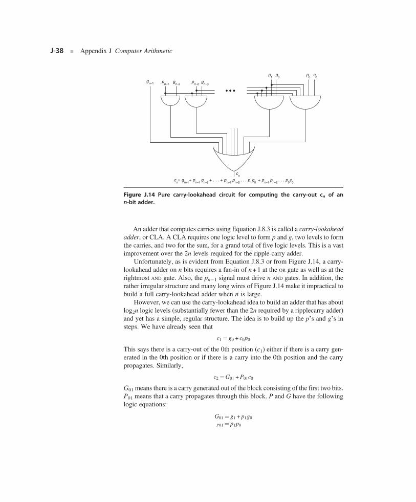
gn–1 p
n–1
cn
gn–2
pn–2
gn–3
p1
g0
p0
c0
cn= g
n–1+ p
n–1g
n–2+ . . . + p
n–1p
n–2 . . . p
1g
0+ p
n–1p
n–2. . . p
0c
0
Figure J.14 Pure carry-lookahead circuit for computing the carry-out cn of ann-bit adder.
J-38 ■ Appendix J Computer Arithmetic
An adder that computes carries using Equation J.8.3 is called a carry-lookaheadadder, or CLA. A CLA requires one logic level to form p and g, two levels to formthe carries, and two for the sum, for a grand total of five logic levels. This is a vastimprovement over the 2n levels required for the ripple-carry adder.
Unfortunately, as is evident from Equation J.8.3 or from Figure J.14, a carry-lookahead adder on n bits requires a fan-in of n+1 at the OR gate as well as at therightmost AND gate. Also, the pn�1 signal must drive n AND gates. In addition, therather irregular structure and many long wires of Figure J.14 make it impractical tobuild a full carry-lookahead adder when n is large.
However, we can use the carry-lookahead idea to build an adder that has aboutlog2n logic levels (substantially fewer than the 2n required by a ripplecarry adder)and yet has a simple, regular structure. The idea is to build up the p’s and g’s insteps. We have already seen that
c1 ¼ g0 + c0p0
This says there is a carry-out of the 0th position (c1) either if there is a carry gen-erated in the 0th position or if there is a carry into the 0th position and the carrypropagates. Similarly,
c2 ¼G01 +P01c0
G01 means there is a carry generated out of the block consisting of the first two bits.P01 means that a carry propagates through this block. P and G have the followinglogic equations:
G01 ¼ g1 + p1g0
P01 ¼ p1p0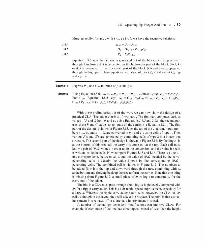
J:8:4
J:8:5
J:8:6
Answer
J.8 Speeding Up Integer Addition ■ J-39
More generally, for any j with i< j, j+1<k, we have the recursive relations:
ck + 1 ¼Gik +Pikci
Gik ¼Gj+ 1,k +Pj+ 1,kGij
Pik ¼PijPj + 1,k
Equation J.8.5 says that a carry is generated out of the block consisting of bits ithrough k inclusive if it is generated in the high-order part of the block (j+1, k)or if it is generated in the low-order part of the block (i,j) and then propagatedthrough the high part. These equations will also hold for i� j<k if we set Gii¼giand Pii¼pi.
Example
Express P03 and G03 in terms of p’s and g’s.Using Equation J.8.6, P03¼P01P23¼P00P11P22P33. Since Pii¼pi, P03¼p0p1p2p3.For G03, Equation J.8.5 says G03¼G23+P23G01¼ (G33+P33G22)+ (P22P33)
(G11+P11G00)¼g3+p3g2+p3p2g1+p3p2p1g0.With these preliminaries out of the way, we can now show the design of apractical CLA. The adder consists of two parts. The first part computes variousvalues of P and G from pi and gi, using Equations J.8.5 and J.8.6; the second partuses these P and G values to compute all the carries via Equation J.8.4. The firstpart of the design is shown in Figure J.15. At the top of the diagram, input num-bers a7… a0 and b7… b0 are converted to p’s and g’s using cells of type 1. Thenvarious P’s and G’s are generated by combining cells of type 2 in a binary treestructure. The second part of the design is shown in Figure J.16. By feeding c0 inat the bottom of this tree, all the carry bits come out at the top. Each cell mustknow a pair of (P,G) values in order to do the conversion, and the value it needsis written inside the cells. Now compare Figures J.15 and J.16. There is a one-to-one correspondence between cells, and the value of (P,G) needed by the carry-generating cells is exactly the value known by the corresponding (P,G)-generating cells. The combined cell is shown in Figure J.17. The numbers tobe added flow into the top and downward through the tree, combining with c0at the bottom and flowing back up the tree to form the carries. Note that one thingis missing from Figure J.17: a small piece of extra logic to compute c8 for thecarry-out of the adder.
The bits in a CLA must pass through about log2 n logic levels, compared with2n for a ripple-carry adder. This is a substantial speed improvement, especially fora large n. Whereas the ripple-carry adder had n cells, however, the CLA has 2ncells, although in our layout they will take n log n space. The point is that a smallinvestment in size pays off in a dramatic improvement in speed.
A number of technology-dependent modifications can improve CLAs. For
example, if each node of the tree has three inputs instead of two, then the height
1 1 1 1 1 1
1
1 1
2
2
2
2
2
a7
b7
a6
b6
a5
b5
a4
b4
a3
b3
a2
b2
a1
b1
a0
b0
p0
g0
p1
g1
g7
p7
G6, 7
P6, 7
G4, 5
P4, 5
G2, 3
P2, 3
G0 ,1
P0 ,1
G4, 7
P4, 7
G0, 3
P0, 3
G0, 7
P0, 7
gi = a
ib
i p
i = a
i + b
i G
i, k = G
j+1, k + P
j+1, k G
i, j
Pi, k
= Pi, j
Pj+1,k
Pi, j
Gi, j
Gj+1, k
ai
bi
Pj+1, k
22
2
Figure J.15 First part of carry-lookahead tree. As signals flow from the top to thebottom, various values of P and G are computed.
c7
c6
c5
c4
c3
c2
c1
c0
p0
g0
p2
g2
P 0, 1
G0, 1
p4
g4
p6
g6
c6
c4
c2
c0
c0
c4
c0
cj+1
= Gi j
+ Pi j
ci
ci
Pi, j
Gi, j
ci
p4, 5
G4, 5
P0, 3
G0, 3
Figure J.16 Second part of carry-lookahead tree. Signals flow from the bottom to thetop, combining with P and G to form the carries.
J-40 ■ Appendix J Computer Arithmetic
of the tree will decrease from log2 n to log3 n. Of course, the cells will be morecomplex and thus might operate more slowly, negating the advantage of thedecreased height. For technologies where rippling works well, a hybrid design
might be better. This is illustrated in Figure J.19. Carries ripple between adders
A A
A
B
B
s7
a7
b7
c7
A A A A A A
B
BBB
+ +
B
s1
a1
b1
s0
a0
b0
c6 c
5c
4c
3c
2c
1c
0
c0
c0
P0, 3
G0, 3
c4
c0
si a
ib
i
si = a
i p
i = a
i + b
ig
i = a
i b
i
gi
pi
ci G
i, kP
i, kc
i
ci
Pi j
Gij
cj +1
Pj +1,k
Gj +1,k
bi
ci
c2
c4c
6
B
Figure J.17 Complete carry-lookahead tree adder. This is the combination ofFigures J.15 and J.16. The numbers to be added enter at the top, flow to the bottomto combine with c0, and then flow back up to compute the sum bits.
J.8 Speeding Up Integer Addition ■ J-41
at the top level, while the “B” boxes are the same as those in Figure J.17. Thisdesign will be faster if the time to ripple between four adders is faster than the timeit takes to traverse a level of “B” boxes. (To make the pattern more clear,Figure J.19 shows a 16-bit adder, so the 8-bit adder of Figure J.17 correspondsto the right half of Figure J.19.)
Carry-Skip Adders
A carry-skip adder sits midway between a ripple-carry adder and a carry-lookahead adder, both in terms of speed and cost. (A carry-skip adder is not calleda CSA, as that name is reserved for carry-save adders.) The motivation for thisadder comes from examining the equations for P and G. For example,
P03 ¼ p0p1p2p3G03 ¼ g3 + p3g2 + p3p2g1 + p3p2p1g0
Computing P is much simpler than computing G, and a carry-skip adder only
computes the P’s. Such an adder is illustrated in Figure J.18. Carries begin rippling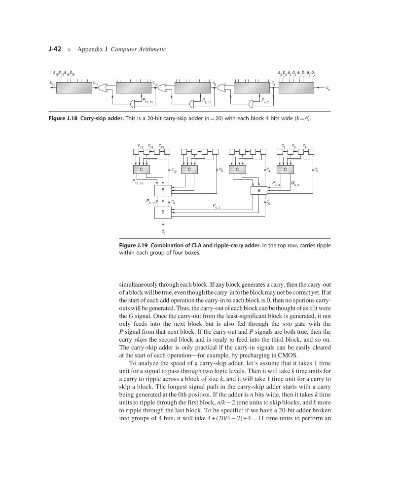
a3
b3
a2
b2
a1
b1
a0
b0
c4
c0
P4, 7
c8
c12
P12, 15 P
8, 11
a19
a18
b19
b18
c16
c20
Figure J.18 Carry-skip adder. This is a 20-bit carry-skip adder (n¼20) with each block 4 bits wide (k¼4).
c15
c14
c13
c12
P12, 15
P8, 15
c8
c0
P0, 7
c8
c4
c0
c0
G0, 3
P0, 3
c1
c2
c3
C
B
B
C C C
B
Figure J.19 Combination of CLA and ripple-carry adder. In the top row, carries ripplewithin each group of four boxes.
J-42 ■ Appendix J Computer Arithmetic
simultaneously through each block. If any block generates a carry, then the carry-outof ablockwill be true, even though the carry-in to theblockmaynot becorrect yet. If atthe start of each add operation the carry-in to each block is 0, then no spurious carry-outswill be generated. Thus, the carry-out of each block can be thought of as if itwerethe G signal. Once the carry-out from the least-significant block is generated, it notonly feeds into the next block but is also fed through the AND gate with theP signal from that next block. If the carry-out and P signals are both true, then thecarry skips the second block and is ready to feed into the third block, and so on.The carry-skip adder is only practical if the carry-in signals can be easily clearedat the start of each operation—for example, by precharging in CMOS.
To analyze the speed of a carry-skip adder, let’s assume that it takes 1 timeunit for a signal to pass through two logic levels. Then it will take k time units fora carry to ripple across a block of size k, and it will take 1 time unit for a carry toskip a block. The longest signal path in the carry-skip adder starts with a carrybeing generated at the 0th position. If the adder is n bits wide, then it takes k timeunits to ripple through the first block, n/k�2 time units to skip blocks, and kmoreto ripple through the last block. To be specific: if we have a 20-bit adder broken
into groups of 4 bits, it will take 4+ (20/4�2)+4¼11 time units to perform an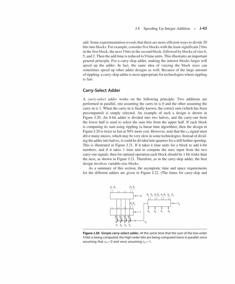
J.8 Speeding Up Integer Addition ■ J-43
add. Some experimentation reveals that there are more efficient ways to divide 20bits into blocks. For example, consider five blocks with the least-significant 2 bitsin the first block, the next 5 bits in the second block, followed by blocks of size 6,5, and 2. Then the add time is reduced to 9 time units. This illustrates an importantgeneral principle. For a carry-skip adder, making the interior blocks larger willspeed up the adder. In fact, the same idea of varying the block sizes cansometimes speed up other adder designs as well. Because of the large amountof rippling, a carry-skip adder is most appropriate for technologies where ripplingis fast.
Carry-Select Adder
A carry-select adder works on the following principle: Two additions areperformed in parallel, one assuming the carry-in is 0 and the other assuming thecarry-in is 1. When the carry-in is finally known, the correct sum (which has beenprecomputed) is simply selected. An example of such a design is shown inFigure J.20. An 8-bit adder is divided into two halves, and the carry-out fromthe lower half is used to select the sum bits from the upper half. If each blockis computing its sum using rippling (a linear time algorithm), then the design inFigure J.20 is twice as fast at 50% more cost. However, note that the c4 signal mustdrive manymuxes, which may be very slow in some technologies. Instead of divid-ing the adder into halves, it could be divided into quarters for a still further speedup.This is illustrated in Figure J.21. If it takes k time units for a block to add k-bitnumbers, and if it takes 1 time unit to compute the mux input from the twocarry-out signals, then for optimal operation each block should be 1 bit wider thanthe next, as shown in Figure J.21. Therefore, as in the carry-skip adder, the bestdesign involves variable-size blocks.
As a summary of this section, the asymptotic time and space requirements
for the different adders are given in Figure J.22. (The times for carry-skip andc0
s0
s1
s2
s3
c4
s4
a4
b4
s5
s6
s7
1
0a
3 b
3 a
2 b
2 a
1 b
1 a
0 b
0
a7 b
7a
4 b
4
Figure J.20 Simple carry-select adder. At the same time that the sum of the low-order4 bits is being computed, the high-order bits are being computed twice in parallel: onceassuming that c4¼0 and once assuming c4¼1.

J.9
c13
c8
c4 c
0
s0
s1
s2
s3
s4
s5
s6
s7
s8
s9
1
00
1
s10
s11
s12
s13
c13
c8
1
s14
s15
s16
s17
s18
0
Figure J.21 Carry-select adder. As soon as the carry-out of the rightmost block isknown, it is used to select the other sum bits.
Figure J.22 Asymptotic time and space requirements for four different types ofadders.
J-44 ■ Appendix J Computer Arithmetic
carry-select come from a careful choice of block size. See Exercise J.26 for thecarry-skip adder.) These different adders shouldn’t be thought of as disjointchoices, but rather as building blocks to be used in constructing an adder. The util-ity of these different building blocks is highly dependent on the technology used.For example, the carry-select adder works well when a signal can drive manymuxes, and the carry-skip adder is attractive in technologies where signals canbe cleared at the start of each operation. Knowing the asymptotic behavior ofadders is useful in understanding them, but relying too much on that behavior isa pitfall. The reason is that asymptotic behavior is only important as n grows verylarge. But n for an adder is the bits of precision, and double precision today is thesame as it was 20 years ago—about 53 bits. Although it is true that as computersget faster, computations get longer—and thus have more rounding error, which in
turn requires more precision—this effect grows very slowly with time.Speeding Up Integer Multiplication and Division
The multiplication and division algorithms presented in Section J.2 are fairly slow,producing 1 bit per cycle (although that cycle might be a fraction of the CPUinstruction cycle time). In this section, we discuss various techniques forhigher-performance multiplication and division, including the division algorithm
used in the Pentium chip.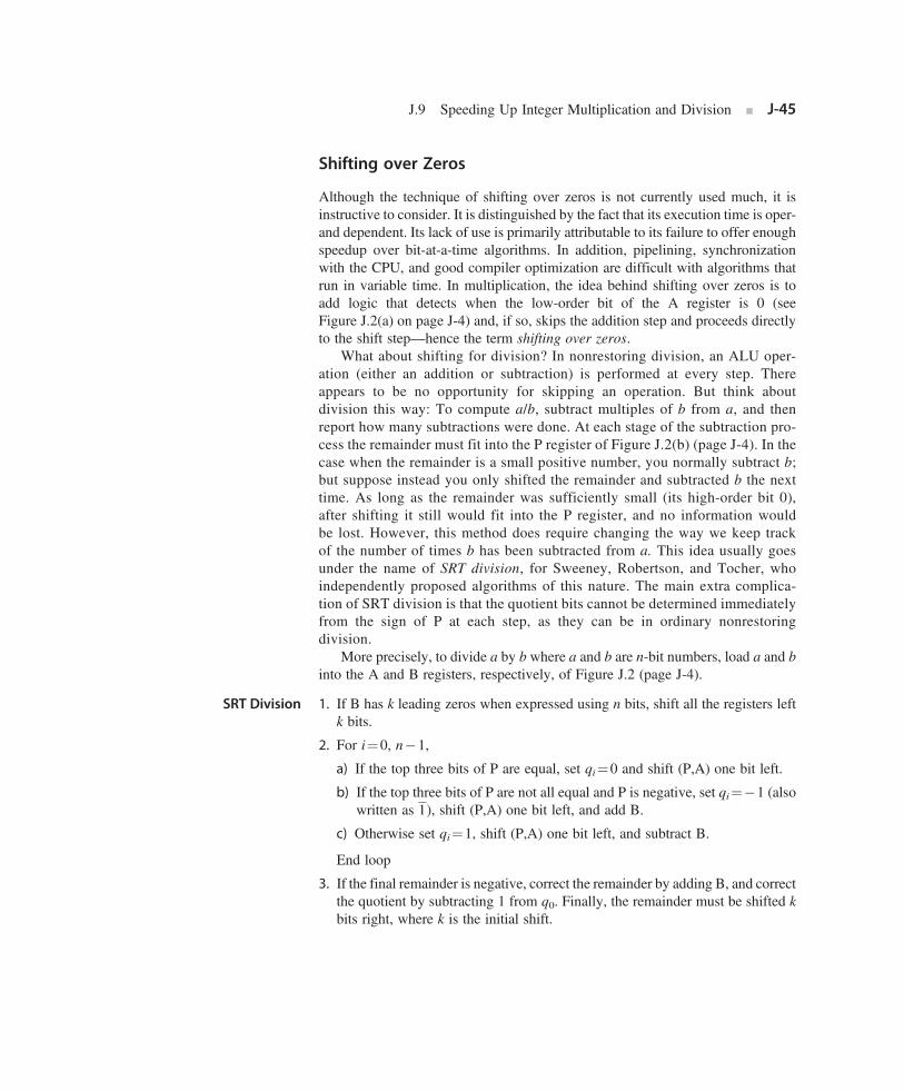
SRT Division
J.9 Speeding Up Integer Multiplication and Division ■ J-45
Shifting over Zeros
Although the technique of shifting over zeros is not currently used much, it isinstructive to consider. It is distinguished by the fact that its execution time is oper-and dependent. Its lack of use is primarily attributable to its failure to offer enoughspeedup over bit-at-a-time algorithms. In addition, pipelining, synchronizationwith the CPU, and good compiler optimization are difficult with algorithms thatrun in variable time. In multiplication, the idea behind shifting over zeros is toadd logic that detects when the low-order bit of the A register is 0 (seeFigure J.2(a) on page J-4) and, if so, skips the addition step and proceeds directlyto the shift step—hence the term shifting over zeros.
What about shifting for division? In nonrestoring division, an ALU oper-ation (either an addition or subtraction) is performed at every step. Thereappears to be no opportunity for skipping an operation. But think aboutdivision this way: To compute a/b, subtract multiples of b from a, and thenreport how many subtractions were done. At each stage of the subtraction pro-cess the remainder must fit into the P register of Figure J.2(b) (page J-4). In thecase when the remainder is a small positive number, you normally subtract b;but suppose instead you only shifted the remainder and subtracted b the nexttime. As long as the remainder was sufficiently small (its high-order bit 0),after shifting it still would fit into the P register, and no information wouldbe lost. However, this method does require changing the way we keep trackof the number of times b has been subtracted from a. This idea usually goesunder the name of SRT division, for Sweeney, Robertson, and Tocher, whoindependently proposed algorithms of this nature. The main extra complica-tion of SRT division is that the quotient bits cannot be determined immediatelyfrom the sign of P at each step, as they can be in ordinary nonrestoringdivision.
More precisely, to divide a by b where a and b are n-bit numbers, load a and b
into the A and B registers, respectively, of Figure J.2 (page J-4).1. If B has k leading zeros when expressed using n bits, shift all the registers leftk bits.
2. For i¼0, n�1,
a) If the top three bits of P are equal, set qi¼0 and shift (P,A) one bit left.
b) If the top three bits of P are not all equal and P is negative, set qi¼�1 (alsowritten as 1), shift (P,A) one bit left, and add B.
c) Otherwise set qi¼1, shift (P,A) one bit left, and subtract B.
End loop
3. If the final remainder is negative, correct the remainder by adding B, and correctthe quotient by subtracting 1 from q0. Finally, the remainder must be shifted k
bits right, where k is the initial shift.
Figure J.23 SRT division of 10002/00112. The quotient bits are shown in bold, usingthe notation 1 for �1.
J-46 ■ Appendix J Computer Arithmetic
Anumerical example is given in Figure J.23. Althoughwe are discussing integerdivision, it helps in explaining the algorithm to imagine the binary point just left ofthe most-significant bit. This changes Figure J.23 from 010002/00112 to 0.10002/.00112. Since the binary point is changed in both the numerator and denominator,the quotient is not affected. The (P,A) register pair holds the remainder and is a two’scomplement number. For example, if P contains 111102 andA¼0, then the remain-der is 1.11102¼�1/8. If r is the value of the remainder, then �1� r<1.
Given these preliminaries, we can now analyze the SRT division algorithm. Thefirst step of the algorithm shifts b so that b�1/2. The rule for which ALU operationto perform is this: If�1/4� r<1/4 (true whenever the top three bits of P are equal),then compute 2r by shifting (P,A) left one bit; if r<0 (and hence r<�1/4, sinceotherwise it would have been eliminated by the first condition), then compute 2r+b by shifting and then adding; if r�1/4 and subtract b from 2r. Using b�1/2,it is easy to check that these rules keep �1/2� r<1/2. For nonrestoring division,we only have jrj�b, and we need P to be n+1 bits wide. But, for SRT division,the bound on r is tighter, namely, �1/2� r<1/2. Thus, we can save a bit by elim-inating the high-order bit of P (and b and the adder). In particular, the test for equalityof the top three bits of P becomes a test on just two bits.
The algorithm might change slightly in an implementation of SRT division.After each ALU operation, the P register can be shifted as many places as necessaryto make either r�1/4 or r<�1/4. By shifting k places, k quotient bits are set equalto zero all at once. For this reason SRT division is sometimes described as one that
keeps the remainder normalized to jrj�1/4.
J.9 Speeding Up Integer Multiplication and Division ■ J-47
Notice that the value of the quotient bit computed in a given step is based onwhich operation is performed in that step (which in turn depends on the result of theoperation from the previous step). This is in contrast to nonrestoring division,where the quotient bit computed in the ith step depends on the result of the oper-ation in the same step. This difference is reflected in the fact that when the finalremainder is negative, the last quotient bit must be adjusted in SRT division,but not in nonrestoring division. However, the key fact about the quotient bitsin SRT division is that they can include 1. Although Figure J.23 shows the quotientbits being stored in the low-order bits of A, an actual implementation can’t do thisbecause you can’t fit the three values �1, 0, 1 into one bit. Furthermore, the quo-tient must be converted to ordinary two’s complement in a full adder. A commonway to do this is to accumulate the positive quotient bits in one register and thenegative quotient bits in another, and then subtract the two registers after all thebits are known. Because there is more than one way to write a number in termsof the digits �1, 0, 1, SRT division is said to use a redundant quotientrepresentation.
The differences between SRT division and ordinary nonrestoring division canbe summarized as follows:
1. ALU decision rule—In nonrestoring division, it is determined by the sign of P;in SRT, it is determined by the two most-significant bits of P.
2. Final quotient—In nonrestoring division, it is immediate from the successivesigns of P; in SRT, there are three quotient digits (1, 0, 1), and the final quotientmust be computed in a full n-bit adder.
3. Speed—SRT division will be faster on operands that produce zero quotient bits.
The simple version of the SRT division algorithm given above does not offerenough of a speedup to be practical in most cases. However, later on in this sectionwe will study variants of SRT division that are quite practical.
Speeding Up Multiplication with a Single Adder
As mentioned before, shifting-over-zero techniques are not used much in currenthardware. We now discuss some methods that are in widespread use. Methods thatincrease the speed of multiplication can be divided into two classes: those that use asingle adder and those that use multiple adders. Let’s first discuss techniques thatuse a single adder.
In the discussion of addition we noted that, because of carry propagation, it isnot practical to perform addition with two levels of logic. Using the cells ofFigure J.17, adding two 64-bit numbers will require a trip through seven cellsto compute the P’s and G’s and seven more to compute the carry bits, which willrequire at least 28 logic levels. In the simple multiplier of Figure J.2 on page J-4,each multiplication step passes through this adder. The amount of computation ineach step can be dramatically reduced by using carry-save adders (CSAs). A carry-
save adder is simply a collection of n independent full adders. A multiplier using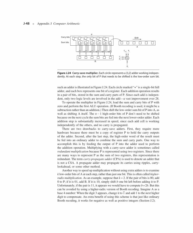
B
A
P
Sum bits
Carry bits
ci
ai
ci+1
si
bi
Shift
+ + + + + +
+
Figure J.24 Carry-save multiplier. Each circle represents a (3,2) adder working indepen-dently. At each step, the only bit of P that needs to be shifted is the low-order sum bit.
J-48 ■ Appendix J Computer Arithmetic
such an adder is illustrated in Figure J.24. Each circle marked “+” is a single-bit fulladder, and each box represents one bit of a register. Each addition operation resultsin a pair of bits, stored in the sum and carry parts of P. Since each add is indepen-dent, only two logic levels are involved in the add—a vast improvement over 28.
To operate the multiplier in Figure J.24, load the sum and carry bits of P withzero and perform the first ALU operation. (If Booth recoding is used, it might be asubtraction rather than an addition.) Then shift the low-order sum bit of P into A, aswell as shifting A itself. The n�1 high-order bits of P don’t need to be shiftedbecause on the next cycle the sum bits are fed into the next lower-order adder. Eachaddition step is substantially increased in speed, since each add cell is workingindependently of the others, and no carry is propagated.
There are two drawbacks to carry-save adders. First, they require morehardware because there must be a copy of register P to hold the carry outputsof the adder. Second, after the last step, the high-order word of the result mustbe fed into an ordinary adder to combine the sum and carry parts. One way toaccomplish this is by feeding the output of P into the adder used to performthe addition operation. Multiplying with a carry-save adder is sometimes calledredundant multiplication because P is represented using two registers. Since thereare many ways to represent P as the sum of two registers, this representation isredundant. The term carry-propagate adder (CPA) is used to denote an adder thatis not a CSA. A propagate adder may propagate its carries using ripples, carry-lookahead, or some other method.
Another way to speed upmultiplication without using extra adders is to examinek low-order bits of A at each step, rather than just one bit. This is often called higher-radix multiplication. As an example, suppose that k¼2. If the pair of bits is 00, add0 to P; if it is 01, add B. If it is 10, simply shift b one bit left before adding it to P.Unfortunately, if the pair is 11, it appears we would have to compute b+2b. But thiscan be avoided by using a higher-radix version of Booth recoding. Imagine A as abase 4 number: When the digit 3 appears, change it to 1 and add 1 to the next higherdigit to compensate. An extra benefit of using this scheme is that just like ordinary
Booth recoding, it works for negative as well as positive integers (Section J.2).
J.9 Speeding Up Integer Multiplication and Division ■ J-49
The precise rules for radix-4 Booth recoding are given in Figure J.25. At the ithmultiply step, the two low-order bits of the A register contain a2i and a2i+1. Thesetwo bits, together with the bit just shifted out (a2i�1), are used to select the multipleof b that must be added to the P register. A numerical example is given inFigure J.26. Another name for this multiplication technique is overlapping triplets,since it looks at 3 bits to determine what multiple of b to use, whereas ordinaryBooth recoding looks at 2 bits.
Besides having more complex control logic, overlapping triplets also requiresthat the P register be 1 bit wider to accommodate the possibility of 2b or�2b beingadded to it. It is possible to use a radix-8 (or even higher) version of Booth recod-ing. In that case, however, it would be necessary to use the multiple 3B as a poten-tial summand. Radix-8 multipliers normally compute 3B once and for all at the
beginning of a multiplication operation.Figure J.25 Multiples of b to use for radix-4 Booth recoding. For example, if the twolow-order bits of the A register are both 1, and the last bit to be shifted out of the Aregister is 0, then the correct multiple is�b, obtained from the second-to-last row ofthe table.
Figure J.26 Multiplication of27 times25 using radix-4 Booth recoding. The columnlabeled L contains the last bit shifted out the right end of A.

J-50 ■ Appendix J Computer Arithmetic
Faster Multiplication with Many Adders
If the space for many adders is available, then multiplication speed can beimproved. Figure J.27 shows a simple array multiplier for multiplying two 5-bitnumbers, using three CSAs and one propagate adder. Part (a) is a block diagramof the kind we will use throughout this section. Parts (b) and (c) show the adder inmore detail. All the inputs to the adder are shown in (b); the actual adders with their
interconnections are shown in (c). Each row of adders in (c) corresponds to a box in(b)
(c)
b0
a1
b0
a0
b0
A
b1
A
b2
A
b3
A
b4
A
b4
a1
b4
a0
b0
a4 b
0 A
b1
A
b2
A
b1
a4
p9
p8
p7
p6
p5
p4
p3
p2
p1
p0
(a)
b4A b
3A
b2A b
1A b
0A
CSA
CSA
CSA
Propagate adder
Figure J.27 An array multiplier. The 5-bit number in A is multiplied by b4b3b2b1b0. Part(a) shows the block diagram, (b) shows the inputs to the array, and (c) expands the arrayto show all the adders.

J.9 Speeding Up Integer Multiplication and Division ■ J-51
(a). The picture is “twisted” so that bits of the same significance are in the samecolumn. In an actual implementation, the array would most likely be laid out asa square instead.
The array multiplier in Figure J.27 performs the same number of additions asthe design in Figure J.24, so its latency is not dramatically different from that of asingle carry-save adder. However, with the hardware in Figure J.27, multiplicationcan be pipelined, increasing the total throughput. On the other hand, although thislevel of pipelining is sometimes used in array processors, it is not used in any of thesingle-chip, floating-point accelerators discussed in Section J.10. Pipelining is dis-cussed in general in Appendix C and by Kogge [1981] in the context of multipliers.
Sometimes the space budgeted on a chip for arithmetic may not hold an arraylarge enough to multiply two double-precision numbers. In this case, a populardesign is to use a two-pass arrangement such as the one shown in Figure J.28.The first pass through the array “retires” 5 bits of B. Then the result of this firstpass is fed back into the top to be combined with the next three summands. Theresult of this second pass is then fed into a CPA. This design, however, losesthe ability to be pipelined.
If arrays require as many addition steps as the much cheaper arrangements inFigures J.2 and J.24, why are they so popular? First of all, using an array has asmaller latency than using a single adder—because the array is a combinationalcircuit, the signals flow through it directly without being clocked. Although thetwo-pass adder of Figure J.28 would normally still use a clock, the cycle timefor passing through k arrays can be less than k times the clock that would be neededfor designs like the ones in Figures J.2 or J.24. Second, the array is amenable tovarious schemes for further speedup. One of them is shown in Figure J.29. Theidea of this design is that two adds proceed in parallel or, to put it another way,
each stream passes through only half the adders. Thus, it runs at almost twiceCSA
CPA
b5A
b2A
b6A
b3A
b7A
b4A
b1A b
0A
CSA
CSA
Figure J.28 Multipass array multiplier. Multiplies two 8-bit numbers with about halfthe hardware that would be used in a one-pass design like that of Figure J.27. At theend of the second pass, the bits flow into the CPA. The inputs used in the first passare marked in bold.
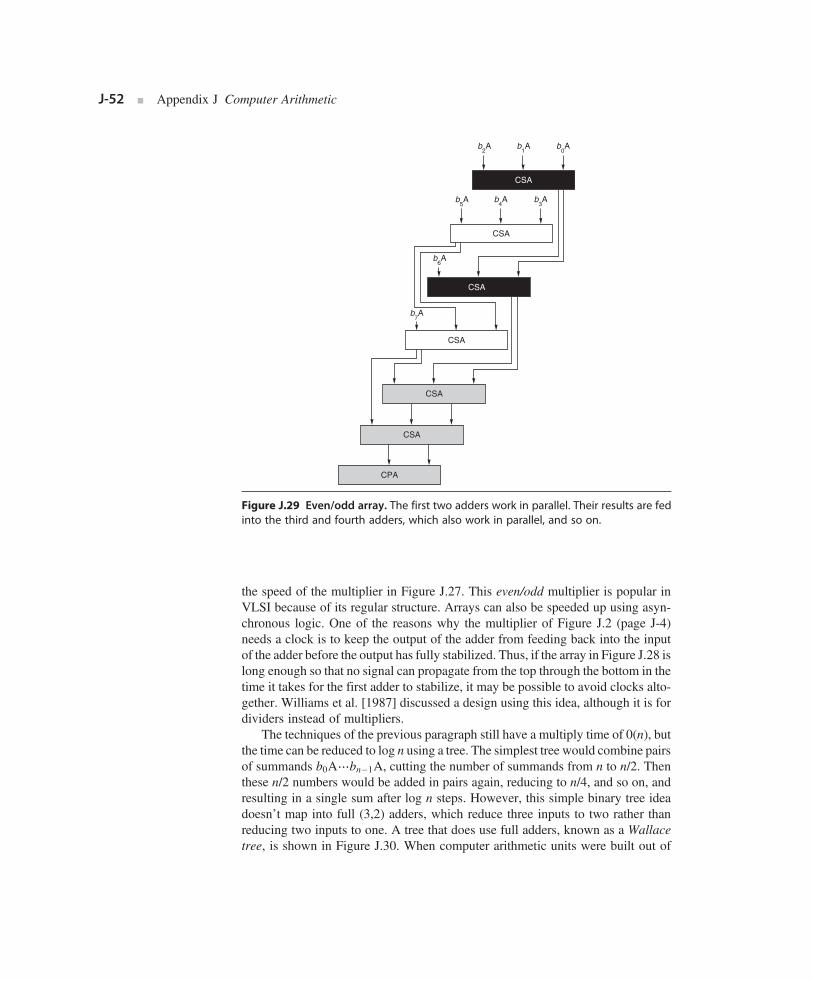
b2A
b4A b
3Ab
5A
b1A b
0A
CSA
CSA
b6A
b7A
CSA
CSA
CSA
CPA
CSA
Figure J.29 Even/odd array. The first two adders work in parallel. Their results are fedinto the third and fourth adders, which also work in parallel, and so on.
J-52 ■ Appendix J Computer Arithmetic
the speed of the multiplier in Figure J.27. This even/odd multiplier is popular inVLSI because of its regular structure. Arrays can also be speeded up using asyn-chronous logic. One of the reasons why the multiplier of Figure J.2 (page J-4)needs a clock is to keep the output of the adder from feeding back into the inputof the adder before the output has fully stabilized. Thus, if the array in Figure J.28 islong enough so that no signal can propagate from the top through the bottom in thetime it takes for the first adder to stabilize, it may be possible to avoid clocks alto-gether. Williams et al. [1987] discussed a design using this idea, although it is fordividers instead of multipliers.
The techniques of the previous paragraph still have a multiply time of 0(n), butthe time can be reduced to log n using a tree. The simplest tree would combine pairsof summands b0A⋯bn�1A, cutting the number of summands from n to n/2. Thenthese n/2 numbers would be added in pairs again, reducing to n/4, and so on, andresulting in a single sum after log n steps. However, this simple binary tree ideadoesn’t map into full (3,2) adders, which reduce three inputs to two rather thanreducing two inputs to one. A tree that does use full adders, known as a Wallace
tree, is shown in Figure J.30. When computer arithmetic units were built out of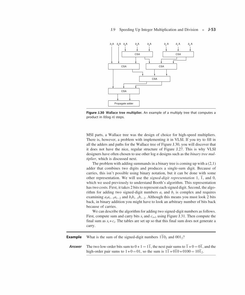
Answer
CSA
CSA
CSA
CSA
b7A b
6A b
5A b
4A b
3A b
2 A b
1 A b
0 A
CSA
CSA
Propagate adder
Figure J.30 Wallace tree multiplier. An example of a multiply tree that computes aproduct in 0(log n) steps.
J.9 Speeding Up Integer Multiplication and Division ■ J-53
MSI parts, a Wallace tree was the design of choice for high-speed multipliers.There is, however, a problem with implementing it in VLSI. If you try to fill inall the adders and paths for the Wallace tree of Figure J.30, you will discover thatit does not have the nice, regular structure of Figure J.27. This is why VLSIdesigners have often chosen to use other log n designs such as the binary tree mul-tiplier, which is discussed next.
The problem with adding summands in a binary tree is coming up with a (2,1)adder that combines two digits and produces a single-sum digit. Because ofcarries, this isn’t possible using binary notation, but it can be done with someother representation. We will use the signed-digit representation 1, 1, and 0,which we used previously to understand Booth’s algorithm. This representationhas two costs. First, it takes 2 bits to represent each signed digit. Second, the algo-rithm for adding two signed-digit numbers ai and bi is complex and requiresexamining aiai�1ai�2 and bibi�1bi�2. Although this means you must look 2 bitsback, in binary addition you might have to look an arbitrary number of bits backbecause of carries.
We can describe the algorithm for adding two signed-digit numbers as follows.First, compute sum and carry bits si and ci+1 using Figure J.31. Then compute thefinal sum as si+ci. The tables are set up so that this final sum does not generate acarry.
Example
What is the sum of the signed-digit numbers 1102 and 0012?The two low-order bits sum to 0 + 1¼ 11, the next pair sums to 1 + 0¼ 01, and the
high-order pair sums to 1+0¼01, so the sum is 11 + 010 + 0100¼ 1012.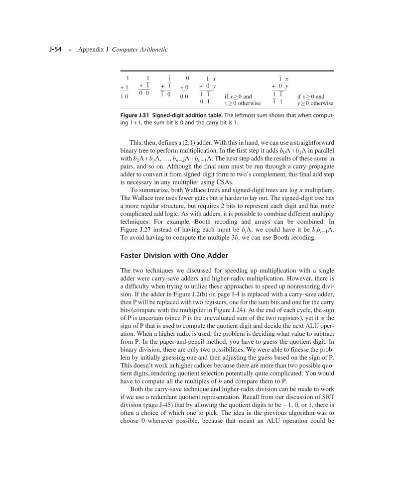
Figure J.31 Signed-digit addition table. The leftmost sum shows that when comput-ing 1+1, the sum bit is 0 and the carry bit is 1.
J-54 ■ Appendix J Computer Arithmetic
This, then, defines a (2,1) adder. With this in hand, we can use a straightforwardbinary tree to perform multiplication. In the first step it adds b0A+b1A in parallelwith b2A+b3A,…, bn�2A+bn�1A. The next step adds the results of these sums inpairs, and so on. Although the final sum must be run through a carry-propagateadder to convert it from signed-digit form to two’s complement, this final add stepis necessary in any multiplier using CSAs.
To summarize, both Wallace trees and signed-digit trees are log n multipliers.The Wallace tree uses fewer gates but is harder to lay out. The signed-digit tree hasa more regular structure, but requires 2 bits to represent each digit and has morecomplicated add logic. As with adders, it is possible to combine different multiplytechniques. For example, Booth recoding and arrays can be combined. InFigure J.27 instead of having each input be biA, we could have it be bibi�1A.To avoid having to compute the multiple 3b, we can use Booth recoding.
Faster Division with One Adder
The two techniques we discussed for speeding up multiplication with a singleadder were carry-save adders and higher-radix multiplication. However, there isa difficulty when trying to utilize these approaches to speed up nonrestoring divi-sion. If the adder in Figure J.2(b) on page J-4 is replaced with a carry-save adder,then P will be replaced with two registers, one for the sum bits and one for the carrybits (compare with the multiplier in Figure J.24). At the end of each cycle, the signof P is uncertain (since P is the unevaluated sum of the two registers), yet it is thesign of P that is used to compute the quotient digit and decide the next ALU oper-ation. When a higher radix is used, the problem is deciding what value to subtractfrom P. In the paper-and-pencil method, you have to guess the quotient digit. Inbinary division, there are only two possibilities. We were able to finesse the prob-lem by initially guessing one and then adjusting the guess based on the sign of P.This doesn’t work in higher radices because there are more than two possible quo-tient digits, rendering quotient selection potentially quite complicated: You wouldhave to compute all the multiples of b and compare them to P.
Both the carry-save technique and higher-radix division can be made to workif we use a redundant quotient representation. Recall from our discussion of SRTdivision (page J-45) that by allowing the quotient digits to be �1, 0, or 1, there isoften a choice of which one to pick. The idea in the previous algorithm was to
choose 0 whenever possible, because that meant an ALU operation could be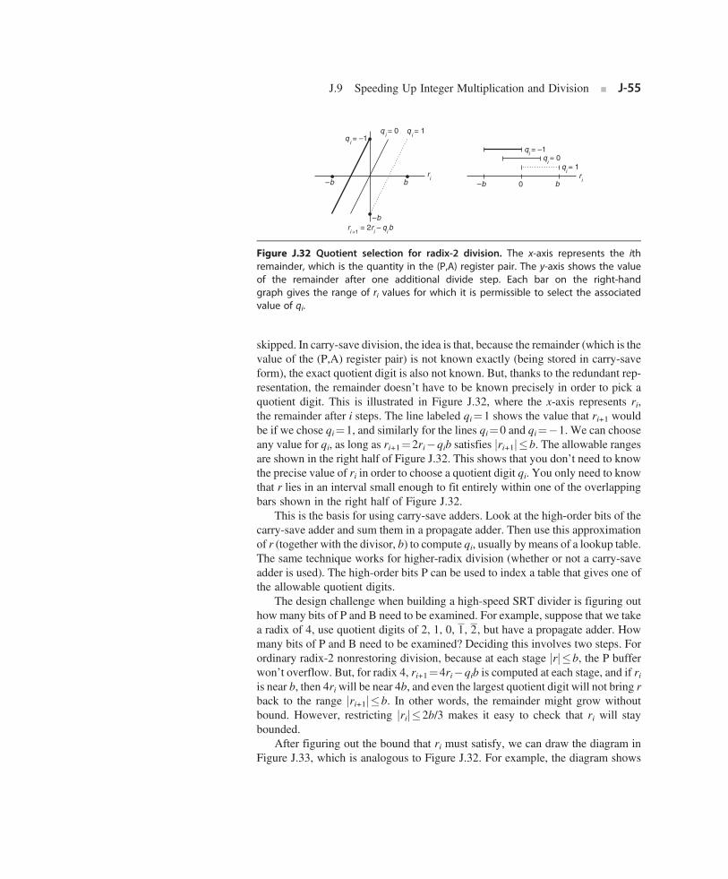
b–b
–b
b–b 0
qi = –1
qi= 0 q
i= 1
qi= –1
qi= 0
qi= 1
ri
ri
ri +1
= 2ri – q
ib
Figure J.32 Quotient selection for radix-2 division. The x-axis represents the ithremainder, which is the quantity in the (P,A) register pair. The y-axis shows the valueof the remainder after one additional divide step. Each bar on the right-handgraph gives the range of ri values for which it is permissible to select the associatedvalue of qi.
J.9 Speeding Up Integer Multiplication and Division ■ J-55
skipped. In carry-save division, the idea is that, because the remainder (which is thevalue of the (P,A) register pair) is not known exactly (being stored in carry-saveform), the exact quotient digit is also not known. But, thanks to the redundant rep-resentation, the remainder doesn’t have to be known precisely in order to pick aquotient digit. This is illustrated in Figure J.32, where the x-axis represents ri,the remainder after i steps. The line labeled qi¼1 shows the value that ri+1 wouldbe if we chose qi¼1, and similarly for the lines qi¼0 and qi¼�1. We can chooseany value for qi, as long as ri+1¼2ri�qib satisfies jri+1j�b. The allowable rangesare shown in the right half of Figure J.32. This shows that you don’t need to knowthe precise value of ri in order to choose a quotient digit qi. You only need to knowthat r lies in an interval small enough to fit entirely within one of the overlappingbars shown in the right half of Figure J.32.
This is the basis for using carry-save adders. Look at the high-order bits of thecarry-save adder and sum them in a propagate adder. Then use this approximationof r (together with the divisor, b) to compute qi, usually by means of a lookup table.The same technique works for higher-radix division (whether or not a carry-saveadder is used). The high-order bits P can be used to index a table that gives one ofthe allowable quotient digits.
The design challenge when building a high-speed SRT divider is figuring outhow many bits of P and B need to be examined. For example, suppose that we takea radix of 4, use quotient digits of 2, 1, 0, 1, 2, but have a propagate adder. Howmany bits of P and B need to be examined? Deciding this involves two steps. Forordinary radix-2 nonrestoring division, because at each stage jrj�b, the P bufferwon’t overflow. But, for radix 4, ri+1¼4ri�qib is computed at each stage, and if riis near b, then 4riwill be near 4b, and even the largest quotient digit will not bring rback to the range jri+1j�b. In other words, the remainder might grow withoutbound. However, restricting jrij�2b/3 makes it easy to check that ri will staybounded.
After figuring out the bound that ri must satisfy, we can draw the diagram in
Figure J.33, which is analogous to Figure J.32. For example, the diagram shows
Answer
2b3
–2b3
2b3
5b12
b3
b6
b12
0
qi = –2 q
i = –1 q
i = 1q
i = 0 q
i = 2
ri
ri +1
= 4ri – q
ib
qi = 2
qi = 1
ri
qi = 0
qi = –2
qi = –1
–2b3
ri +1
Figure J.33 Quotient selection for radix-4 division with quotient digits22,21, 0, 1, 2.
J-56 ■ Appendix J Computer Arithmetic
that if ri is between (1/12)b and (5/12)b, we can pick q¼1, and so on. Or, to put itanother way, if r/b is between 1/12 and 5/12, we can pick q¼1. Suppose thedivider examines 5 bits of P (including the sign bit) and 4 bits of b (ignoringthe sign, since it is always nonnegative). The interesting case is when the high bitsof P are 00011xxx⋯, while the high bits of b are 1001xxx⋯. Imagine the binarypoint at the left end of each register. Since we truncated, r (the value of Pconcatenated with A) could have a value from 0.00112 to 0.01002, and b couldhave a value from .10012 to .10102. Thus, r/b could be as small as 0.00112/.10102 or as large as 0.01002/.10012, but 0.00112/.10102¼3/10<1/3 wouldrequire a quotient bit of 1, while 0.01002/.10012¼4/9>5/12 would require a quo-tient bit of 2. In other words, 5 bits of P and 4 bits of b aren’t enough to pick aquotient bit. It turns out that 6 bits of P and 4 bits of b are enough. This can beverified by writing a simple program that checks all the cases. The output of sucha program is shown in Figure J.34.
Example
Using 8-bit registers, compute 149/5 using radix-4 SRT division.Follow the SRT algorithm on page J-45, but replace the quotient selection rule in
step 2 with one that uses Figure J.34. See Figure J.35.The Pentium uses a radix-4 SRT division algorithm like the one just presented,except that it uses a carry-save adder. Exercises J.34(c) and J.35 explore this indetail. Although these are simple cases, all SRT analyses proceed in the sameway. First compute the range of ri, then plot ri against ri+1 to find the quotientranges, and finally write a program to compute how many bits are necessary.(It is sometimes also possible to compute the required number of bits analytically.)
Various details need to be considered in building a practical SRT divider.
J.10
Figure J.34 Quotient digits for radix-4 SRT division with a propagate adder. The toprow says that if the high-order 4 bits of b are 10002¼8, and if the top 6 bits of P arebetween 1101002¼�12 and 1110012¼�7, then �2 is a valid quotient digit.
J.10 Putting It All Together ■ J-57
For example, the quotient lookup table has a fairly regular structure, which means itis usually cheaper to encode it as a PLA rather than in ROM. For more details about
SRT division, see Burgess and Williams [1995].Putting It All Together
In this section, we will compare the Weitek 3364, the MIPS R3010, and the TexasInstruments 8847 (see Figures J.36 and J.37). In many ways, these are ideal chips
to compare. They each implement the IEEE standard for addition, subtraction,
Figure J.35 Example of radix-4 SRT division. Division of 149 by 5.
Figure J.36 Summary of the three floating-point chips discussed in this section. Thecycle times are for production parts available in June 1989. The cycle counts are fordouble-precision operations.
J-58 ■ Appendix J Computer Arithmetic

Figure J.37 Chip layout for the TI 8847, MIPS R3010, and Weitek 3364. In the left-hand columns are the photo-micrographs; the right-hand columns show the corresponding floor plans.
(Continued)
J.10 Putting It All Together ■ J-59

Figure J.37 (Continued)
J-60 ■ Appendix J Computer Arithmetic
multiplication, and division on a single chip. All were introduced in 1988 and runwith a cycle time of about 40 nanoseconds. However, as we will see, they use quitedifferent algorithms. The Weitek chip is well described in Birman et al. [1990], theMIPS chip is described in less detail in Rowen, Johnson, and Ries [1988], anddetails of the TI chip can be found in Darley et al. [1989].
These three chips have a number of things in common. They perform additionand multiplication in parallel, and they implement neither extended precision nor aremainder step operation. (Recall from Section J.6 that it is easy to implement theIEEE remainder function in software if a remainder step instruction is available.)The designers of these chips probably decided not to provide extended precisionbecause the most influential users are those who run portable codes, which can’trely on extended precision. However, as we have seen, extended precision canmake for faster and simpler math libraries.
In the summary of the three chips given in Figure J.36, note that a higher tran-sistor count generally leads to smaller cycle counts. Comparing the cycles/op num-bers needs to be done carefully, because the figures for the MIPS chip are those fora complete system (R3000/3010 pair), while the Weitek and TI numbers are forstand-alone chips and are usually larger when used in a complete system.
The MIPS chip has the fewest transistors of the three. This is reflected in the
fact that it is the only chip of the three that does not have any pipelining or hardware
J.10 Putting It All Together ■ J-61
square root. Further, the multiplication and addition operations are not completelyindependent because they share the carry-propagate adder that performs the finalrounding (as well as the rounding logic).
Addition on the R3010 uses a mixture of ripple, CLA, and carry-select. Acarry-select adder is used in the fashion of Figure J.20 (page J-43). Within eachhalf, carries are propagated using a hybrid ripple-CLA scheme of the type indicatedin Figure J.19 (page J-42). However, this is further tuned by varying the size ofeach block, rather than having each fixed at 4 bits (as they are in Figure J.19).The multiplier is midway between the designs of Figures J.2 (page J-4) andJ.27 (page J-50). It has an array just large enough so that output can be fed backinto the input without having to be clocked. Also, it uses radix-4 Booth recodingand the even/odd technique of Figure J.29 (page J-52). The R3010 can do a divideand multiply in parallel (like the Weitek chip but unlike the TI chip). The divider isa radix-4 SRTmethod with quotient digits�2,�1, 0, 1, and 2, and is similar to thatdescribed in Taylor [1985]. Double-precision division is about four times slowerthan multiplication. The R3010 shows that for chips using an 0(n) multiplier, anSRT divider can operate fast enough to keep a reasonable ratio between multiplyand divide.
The Weitek 3364 has independent add, multiply, and divide units. It also usesradix-4 SRT division. However, the add and multiply operations on the Weitekchip are pipelined. The three addition stages are (1) exponent compare, (2) addfollowed by shift (or vice versa), and (3) final rounding. Stages (1) and (3) takeonly a half-cycle, allowing the whole operation to be done in two cycles, eventhough there are three pipeline stages. The multiplier uses an array of the styleof Figure J.28 but uses radix-8 Booth recoding, which means it must compute 3times the multiplier. The three multiplier pipeline stages are (1) compute 3b,(2) pass through array, and (3) final carry-propagation add and round. Single pre-cision passes through the array once, double precision twice. Like addition, thelatency is two cycles.
The Weitek chip uses an interesting addition algorithm. It is a variant on thecarry-skip adder pictured in Figure J.18 (page J-42). However, Pij, which is the log-ical AND of many terms, is computed by rippling, performing one AND perripple. Thus, while the carries propagate left within a block, the value of Pij is prop-agating right within the next block, and the block sizes are chosen so that both wavescomplete at the same time. Unlike theMIPS chip, the 3364 has hardware square root,which shares the divide hardware. The ratio of double-precision multiply to divide is2:17. The large disparity between multiply and divide is due to the fact that multi-plication uses radix-8 Booth recoding, while division uses a radix-4 method. In theMIPS R3010, multiplication and division use the same radix.
The notable feature of the TI 8847 is that it does division by iteration (using theGoldschmidt algorithm discussed in Section J.6). This improves the speed of divi-sion (the ratio of multiply to divide is 3:11), but means that multiplication and divi-sion cannot be done in parallel as on the other two chips. Addition has a two-stagepipeline. Exponent compare, fraction shift, and fraction addition are done in the
first stage, normalization and rounding in the second stage. Multiplication uses
J.11
Fallacy
Fallacy
Pitfall
Pitfall
J-62 ■ Appendix J Computer Arithmetic
a binary tree of signed-digit adders and has a three-stage pipeline. The first stagepasses through the array, retiring half the bits; the second stage passes through thearray a second time; and the third stage converts from signed-digit form to two’scomplement. Since there is only one array, a new multiply operation can only beinitiated in every other cycle. However, by slowing down the clock, two passesthrough the array can be made in a single cycle. In this case, a new multiplicationcan be initiated in each cycle. The 8847 adder uses a carry-select algorithm ratherthan carry-lookahead. As mentioned in Section J.6, the TI carries 60 bits of pre-cision in order to do correctly rounded division.
These three chips illustrate the different trade-offs made by designers with sim-ilar constraints. One of the most interesting things about these chips is the diversityof their algorithms. Each uses a different add algorithm, as well as a different mul-tiply algorithm. In fact, Booth recoding is the only technique that is universally
used by all the chips.Fallacies and Pitfalls
Underflows rarely occur in actual floating-point application code
Although most codes rarely underflow, there are actual codes that underflow fre-quently. SDRWAVE [Kahaner 1988], which solves a one-dimensional wave equa-tion, is one such example. This program underflows quite frequently, even whenfunctioning properly. Measurements on one machine show that adding hardware
support for gradual underflow would cause SDRWAVE to run about 50% faster.Conversions between integer and floating point are rare
In fact, in spice they are as frequent as divides. The assumption that conversionsare rare leads to a mistake in the SPARC version 8 instruction set, which does not
provide an instruction to move from integer registers to floating-point registers.Don’t increase the speed of a floating-point unit without increasing its memorybandwidth
A typical use of a floating-point unit is to add two vectors to produce a third vector.If these vectors consist of double-precision numbers, then each floating-pointadd will use three operands of 64 bits each, or 24 bytes of memory. The memorybandwidth requirements are even greater if the floating-point unit can perform
addition and multiplication in parallel (as most do).�x is not the same as 0�x
This is a fine point in the IEEE standard that has tripped up some designers.Because floating-point numbers use the sign magnitude system, there are twozeros, +0 and �0. The standard says that 0�0¼+0, whereas� (0)¼�0. Thus,
�x is not the same as 0�x when x¼0.
J.12 Historical Perspective and References ■ J-63
J.12
Historical Perspective and ReferencesThe earliest computers used fixed point rather than floating point. In “PreliminaryDiscussion of the Logical Design of an Electronic Computing Instrument,” Burks,Goldstine, and von Neumann [1946] put it like this:
There appear to be two major purposes in a “floating” decimal point system both ofwhich arise from the fact that the number of digits in a word is a constant fixed bydesign considerations for each particular machine. The first of these purposes is toretain in a sum or product as many significant digits as possible and the second ofthese is to free the human operator from the burden of estimating and inserting intoa problem “scale factors”—multiplicative constants which serve to keep numberswithin the limits of the machine.There is, of course, no denying the fact that human time is consumed in arrang-
ing for the introduction of suitable scale factors. We only argue that the time soconsumed is a very small percentage of the total time we will spend in preparingan interesting problem for our machine. The first advantage of the floating pointis, we feel, somewhat illusory. In order to have such a floating point, one mustwaste memory capacity that could otherwise be used for carrying more digitsper word. It would therefore seem to us not at all clear whether the modest advan-tages of a floating binary point offset the loss of memory capacity and theincreased complexity of the arithmetic and control circuits.
This enables us to see things from the perspective of early computer designers,who believed that saving computer time and memory were more important thansaving programmer time.
The original papers introducing the Wallace tree, Booth recoding, SRT divi-sion, overlapped triplets, and so on are reprinted in Swartzlander [1990]. A goodexplanation of an early machine (the IBM 360/91) that used a pipelined Wallacetree, Booth recoding, and iterative division is in Anderson et al. [1967]. A discus-sion of the average time for single-bit SRT division is in Freiman [1961]; this is oneof the few interesting historical papers that does not appear in Swartzlander.
The standard book of Mead and Conway [1980] discouraged the use of CLAsas not being cost effective in VLSI. The important paper by Brent and Kung [1982]helped combat that view. An example of a detailed layout for CLAs can be found inNgai and Irwin [1985] or in Weste and Eshraghian [1993], and a more theoreticaltreatment is given by Leighton [1992]. Takagi, Yasuura, and Yajima [1985] pro-vide a detailed description of a signed-digit tree multiplier.
Before the ascendancy of IEEE arithmetic, many different floating-point for-mats were in use. Three important ones were used by the IBM 370, the DEC VAX,and the Cray. Here is a brief summary of these older formats. The VAX format isclosest to the IEEE standard. Its single-precision format (F format) is like IEEEsingle precision in that it has a hidden bit, 8 bits of exponent, and 23 bits of fraction.However, it does not have a sticky bit, which causes it to round halfway cases up
instead of to even. The VAX has a slightly different exponent range from IEEE
J-64 ■ Appendix J Computer Arithmetic
single: Emin is �128 rather than �126 as in IEEE, and Emax is 126 instead of 127.The main differences between VAX and IEEE are the lack of special values andgradual underflow. The VAX has a reserved operand, but it works like a signalingNaN: It traps whenever it is referenced. Originally, the VAX’s double precision(D format) also had 8 bits of exponent. However, as this is too small for manyapplications, a G format was added; like the IEEE standard, this format has 11 bitsof exponent. The VAX also has an H format, which is 128 bits long.
The IBM370 floating-point format uses base 16 rather than base 2. Thismeans itcannot use a hidden bit. In single precision, it has 7 bits of exponent and 24 bits (6 hexdigits) of fraction. Thus, the largest representable number is 1627¼24�27¼229,compared with 228 for IEEE. However, a number that is normalized in the hexadec-imal sense only needs to have a nonzero leading digit.When interpreted in binary, thethreemost-significant bits could be zero. Thus, there are potentially fewer than24bitsof significance. The reason for using the higher base was to minimize the amount ofshifting required when adding floating-point numbers. However, this is less signifi-cant in current machines, where the floating-point add time is usually fixed indepen-dently of the operands. Another difference between 370 arithmetic and IEEEarithmetic is that the 370 has neither a round digit nor a sticky digit, which effectivelymeans that it truncates rather than rounds. Thus, inmany computations, the resultwillsystematically be too small. Unlike theVAXand IEEE arithmetic, every bit pattern isa valid number. Thus, library routinesmust establish conventions forwhat to return incase of errors. In the IBM FORTRAN library, for example,
ffiffiffiffiffiffiffi�4p
returns 2!Arithmetic on Cray computers is interesting because it is driven by a motiva-
tion for the highest possible floating-point performance. It has a 15-bit exponentfield and a 48-bit fraction field. Addition on Cray computers does not have a guarddigit, and multiplication is even less accurate than addition. Thinking of multipli-cation as a sum of p numbers, each 2p bits long, Cray computers drop the low-orderbits of each summand. Thus, analyzing the exact error characteristics of the mul-tiply operation is not easy. Reciprocals are computed using iteration, and divisionof a by b is done by multiplying a times 1/b. The errors in multiplication and recip-rocation combine to make the last three bits of a divide operation unreliable. Atleast Cray computers serve to keep numerical analysts on their toes!
The IEEE standardization process began in 1977, inspired mainly byW. Kahanand based partly on Kahan’s work with the IBM 7094 at the University of Toronto[Kahan 1968]. The standardization process was a lengthy affair, with gradualunderflow causing the most controversy. (According to Cleve Moler, visitors tothe United States were advised that the sights not to be missed were Las Vegas,the Grand Canyon, and the IEEE standards committee meeting.) The standardwas finally approved in 1985. The Intel 8087 was the first major commercial IEEEimplementation and appeared in 1981, before the standard was finalized. It con-tains features that were eliminated in the final standard, such as projective bits.According to Kahan, the length of double-extended precision was based on whatcould be implemented in the 8087. Although the IEEE standard was not based onany existing floating-point system, most of its features were present in some other
system. For example, the CDC 6600 reserved special bit patterns for INDEFINITE
J.12 Historical Perspective and References ■ J-65
and INFINITY, while the idea of denormal numbers appears in Goldberg [1967] aswell as in Kahan [1968]. Kahan was awarded the 1989 Turing prize in recognitionof his work on floating point.
Although floating point rarely attracts the interest of the general press, news-papers were filled with stories about floating-point division in November 1994. Abug in the division algorithm used on all of Intel’s Pentium chips had just come tolight. It was discovered by Thomas Nicely, a math professor at Lynchburg Collegein Virginia. Nicely found the bug when doing calculations involving reciprocals ofprime numbers. News of Nicely’s discovery first appeared in the press on the frontpage of the November 7 issue of Electronic Engineering Times. Intel’s immediateresponse was to stonewall, asserting that the bug would only affect theoreticalmathematicians. Intel told the press, “This doesn’t even qualify as an errata… evenif you’re an engineer, you’re not going to see this.”
Under more pressure, Intel issued a white paper, dated November 30, explain-ing why they didn’t think the bug was significant. One of their arguments wasbased on the fact that if you pick two floating-point numbers at random and divideone into the other, the chance that the resulting quotient will be in error is about 1 in9 billion. However, Intel neglected to explain why they thought that the typicalcustomer accessed floating-point numbers randomly.
Pressure continued to mount on Intel. One sore point was that Intel had knownabout the bug before Nicely discovered it, but had decided not to make it public.Finally, on December 20, Intel announced that they would unconditionally replaceany Pentium chip that used the faulty algorithm and that they would take an unspe-cified charge against earnings, which turned out to be $300 million.
The Pentium uses a simple version of SRT division as discussed in Section J.9.The bug was introduced when they converted the quotient lookup table to a PLA.Evidently there were a few elements of the table containing the quotient digit 2 thatIntel thought would never be accessed, and they optimized the PLA design usingthis assumption. The resulting PLA returned 0 rather than 2 in these situations.However, those entries were really accessed, and this caused the division bug.Even though the effect of the faulty PLA was to cause 5 out of 2048 table entriesto be wrong, the Pentium only computes an incorrect quotient 1 out of 9 billion
times on random inputs. This is explored in Exercise J.34.References
Anderson, S.F., Earle, J.G., Goldschmidt, R.E., Powers, D.M., 1967. The IBM System/360 Model 91:Floating-point execution unit. IBM J. Research and Development 11, 34–53. Reprinted inSwartzlander [1990]. Good description of an early high-performance floating-point unit that useda pipelined Wallace tree multiplier and iterative division.
Bell, C.G., Newell, A., 1971. Computer Structures: Readings and Examples. McGraw-Hill, New York.Birman, M., Samuels, A., Chu, G., Chuk, T., Hu, L., McLeod, J., Barnes, J., 1990. Developing the
WRL3170/3171 SPARC floating-point coprocessors. IEEE Micro 10 (1), 55–64. These chips havethe same floating-point core as the Weitek 3364, and this paper has a fairly detailed description of
that floating-point design.
J-66 ■ Appendix J Computer Arithmetic
Brent, R.P., Kung, H.T., 1982. A regular layout for parallel adders. IEEE Trans. on ComputersC-31, 260–264. This is the paper that popularized CLAs in VLSI.
Burgess, N., Williams, T., 1995. Choices of operand truncation in the SRT division algorithm. IEEETrans. on Computers 44, 7. Analyzes how many bits of divisor and remainder need to be examinedin SRT division.
Burks, A.W., Goldstine, H.H., von Neumann, J., 1946. Preliminary discussion of the logical design ofan electronic computing instrument. In: Aspray, W., Burks, A. (Eds.), Papers of John von Neumann.Report to the U.S. Army Ordnance Department, p. 1; also appears. MIT Press, Cambridge, Mass,pp. 97–146. Tomash Publishers, Los Angeles, 1987.
Cody, W.J., Coonen, J.T., Gay, D.M., Hanson, K., Hough, D., Kahan, W., Karpinski, R., Palmer, J.,Ris, F.N., Stevenson, D., 1984. A proposed radix- and word-length-independent standard forfloating-point arithmetic. IEEE Micro 4 (4), 86–100. Contains a draft of the 854 standard, whichis more general than 754. The significance of this article is that it contains commentary on the stan-dard, most of which is equally relevant to 754. However, be aware that there are some differencesbetween this draft and the final standard.
Coonen, J., 1984. Contributions to a proposed standard for binary floating point arithmetic. Ph.D. thesis.University of California–Berkeley. The only detailed discussion of how rounding modes can be usedto implement efficient binary decimal conversion.
Darley, H.M., et al., 1989. Floating point/integer processor with divide and square root functions. U.S.Patent. 4 (878,190) October 31, 1989. Pretty readable as patents go. Gives a high-level view of the TI8847 chip, but doesn’t have all the details of the division algorithm.
Demmel, J.W., Li, X., 1994. Faster numerical algorithms via exception handling. IEEE Trans. onComputers 43 (8), 983–992. A good discussion of how the features unique to IEEE floating pointcan improve the performance of an important software library.
Freiman, C.V., 1961. Statistical analysis of certain binary division algorithms. Proc. IRE 49 (1), 91–103.Contains an analysis of the performance of shifting-over-zeros SRT division algorithm.
Goldberg, D., 1991. What every computer scientist should know about floating-point arithmetic.Computing Surveys 23 (1), 5–48. Contains an in-depth tutorial on the IEEE standard from the soft-ware point of view.
Goldberg, I.B., 1967. 27 bits are not enough for 8-digit accuracy. Comm. ACM 10 (2), 105–106. Thispaper proposes using hidden bits and gradual underflow.
Gosling, J.B., 1980. Design of Arithmetic Units for Digital Computers. Springer-Verlag, New York.A concise, well-written book, although it focuses on MSI designs.
Hamacher, V.C., Vranesic, Z.G., Zaky, S.G., 1984. Computer Organization, 2nd ed.McGraw-Hill, NewYork. Introductory computer architecture book with a good chapter on computer arithmetic.
Hwang, K., 1979. Computer Arithmetic: Principles, Architecture, and Design. Wiley, New York. Thisbook contains the widest range of topics of the computer arithmetic books.
IEEE, 1985. IEEE standard for binary floating-point arithmetic. SIGPLAN Notices 22 (2), 9–25. IEEE754 is reprinted here.
Kahan,W., 1968. 7094-II system support for numerical analysis. SHARE Secretarial Distribution. SSD-159. This system had many features that were incorporated into the IEEE floating-point standard.
Kahaner, D.K., 1988. Benchmarks for ‘real’ programs. SIAM News.(November).. The benchmark pre-sented in this article turns out to cause many underflows.
Knuth, D., 1981. 2nd ed. The Art of Computer Programming.Vol. II. Addison-Wesley, Reading, Mass.Has a section on the distribution of floating-point numbers.
Kogge, P., 1981. The Architecture of Pipelined Computers. McGraw-Hill, New York. Has a brief dis-cussion of pipelined multipliers.
Kohn, L., Fu, S.-W., 1989. A 1,000,000 transistor microprocessor. In: IEEE Int’l. Solid-State CircuitsConf. Digest of Technical Papers, pp. 54–55. There are several articles about the i860, but this onecontains the most details about its floating-point algorithms.
Koren, I., 1989. Computer Arithmetic Algorithms. Prentice Hall, Englewood Cliffs, N.J..Leighton, F.T., 1992. Introduction to Parallel Algorithms andArchitectures: Arrays. Trees, Hypercubes,
Morgan Kaufmann, San Francisco. This is an excellent book, with emphasis on the complexity anal-
ysis of algorithms. Section 1.2.1 has a nice discussion of carry-lookahead addition on a tree.
Exercises ■ J-67
Magenheimer, D.J., Peters, L., Pettis, K.W., Zuras, D., 1988. Integer multiplication and division on theHP Precision architecture. IEEE Trans. on Computers 37 (8), 980–990. Gives rationale for theinteger- and divide-step instructions in the Precision architecture.
Markstein, P.W., 1990. Computation of elementary functions on the IBMRISC System/6000 processor.IBM J. of Research and Development 34 (1), 111–119. Explains how to use fused muliply-add tocompute correctly rounded division and square root.
Mead, C., Conway, L., 1980. Introduction to VLSI Systems. Addison-Wesley, Reading, Mass.Montoye, R.K., Hokenek, E., Runyon, S.L., 1990. Design of the IBMRISC System/6000 floating-point
execution. IBM J. of Research and Development 34 (1), 59–70. Describes one implementation offused multiply-add.
Ngai, T.-F., Irwin, M.J., 1985. Regular, area-time efficient carry-lookahead adders. In: Proc. SeventhIEEE Symposium on Computer Arithmetic, pp. 9–15. Describes a CLA like that of Figure J.17,where the bits flow up and then come back down.
Patterson, D.A., Hennessy, J.L., 2009. Computer Organization and Design: The Hardware/SoftwareInterface, 4th Edition Morgan Kaufmann, San Francisco. Chapter 3 is a gentler introduction tothe first third of this appendix.
Peng, V., Samudrala, S., Gavrielov, M., 1987. On the implementation of shifters, multipliers, anddividers in VLSI floating point units. In: Proc. Eighth IEEE Symposium on Computer Arithmetic,pp. 95–102. Highly recommended survey of different techniques actually used in VLSI designs.
Rowen, C., Johnson, M., Ries, P., 1988. The MIPS R3010 floating-point coprocessor. IEEE Micro53–62 (June).
Santoro, M.R., Bewick, G., Horowitz, M.A., 1989. Rounding algorithms for IEEE multipliers. In: Proc.Ninth IEEE Symposium onComputer Arithmetic, pp. 176–183.A very readable discussion of how toefficiently implement rounding for floating-point multiplication.
Scott, N.R., 1985. Computer Number Systems and Arithmetic. Prentice Hall, Englewood Cliffs, N.J.Swartzlander, E. (Ed.), 1990. Computer Arithmetic. IEEEComputer Society Press, Los Alamitos, Calif.
A collection of historical papers in two volumes.Takagi, N., Yasuura, H., Yajima, S., 1985. High-speed VLSI multiplication algorithm with a redundant
binary addition tree. IEEE Trans. on Computers C-34 (9), 789–796. A discussion of the binary treesigned multiplier that was the basis for the design used in the TI 8847.
Taylor, G.S., 1981. Compatible hardware for division and square root. In: Proc. Fifth IEEE Symposiumon Computer Arithmetic, May 18–19, 1981. Ann Arbor, Mich, pp. 127–134. Good discussion of aradix-4 SRT division algorithm.
Taylor, G.S., 1985. Radix 16 SRT dividers with overlapped quotient selection stages. In: Proc. SeventhIEEE Symposium on Computer Arithmetic, June 4–6, 1985, pp. 64–71 Urbana, Ill..Describes a verysophisticated high-radix division algorithm.
Weste, N., Eshraghian, K., 1993. Principles of CMOS VLSI Design: A Systems Perspective, 2nd ed.Addison-Wesley, Reading, Mass. This textbook has a section on the layouts of various kinds ofadders.
Williams, T.E., Horowitz, M., Alverson, R.L., Yang, T.S., 1987. A self-timed chip for division.In: Advanced Research in VLSI, Proc. 1987 Stanford Conf. MIT Press, Cambridge, Mass.Describesa divider that tries to get the speed of a combinational design without using the area that would be
required by one.Exercises
J.1 [12]< J.2>Using n bits, what is the largest and smallest integer that can be repre-sented in the two’s complement system?
J.2 [20/25]< J.2> In the subsection “Signed Numbers” (page J-7), it was stated thattwo’s complement overflows when the carry into the high-order bit position is dif-
ferent from the carry-out from that position.
J.11
J-68 ■ Appendix J Computer Arithmetic
a. [20]< J.2>Give examples of pairs of integers for all four combinations ofcarry-in and carry-out. Verify the rule stated above.
b. [25]< J.2>Explain why the rule is always true.
J.3 [12]< J.2>Using 4-bit binary numbers, multiply�8��8 using Booth recoding.
J.4 [15]< J.2>Equations J.2.1 and J.2.2 are for adding two n-bit numbers.Derive similar equations for subtraction, where there will be a borrow insteadof a carry.
J.5 [25]< J.2>On a machine that doesn’t detect integer overflow in hardware, showhow you would detect overflow on a signed addition operation in software.
J.6 [15/15/20]< J.3>Represent the following numbers as single-precision and
double-precision IEEE floating-point numbers:a. [15]< J.3>10.
b. [15]< J.3>10.5.
c. [20]< J.3>0.1.
J.7 [12/12/12/12/12]< J.3>Below is a list of floating-point numbers. In single preci-sion, write down each number in binary, in decimal, and give its representation in
IEEE arithmetic.a. [12]< J.3>The largest number less than 1.
b. [12]< J.3>The largest number.
c. [12]< J.3>The smallest positive normalized number.
d. [12]< J.3>The largest denormal number.
e. [12]< J.3>The smallest positive number.
J.8 [15]< J.3> Is the ordering of nonnegative floating-point numbers the same as inte-gers when denormalized numbers are also considered?
J.9 [20]< J.3>Write a program that prints out the bit patterns used to representfloating-point numbers on your favorite computer. What bit pattern is usedfor NaN?
J.10 [15]< J.4>Using p¼4, show how the binary floating-point multiply algorithmcomputes the product of 1.875�1.875.
[12/10]< J.4>Concerning the addition of exponents in floating-point multiply:
a. [12]< J.4>What would the hardware that implements the addition of expo-nents look like?
b. [10]< J.4> If the bias in single precision were 129 instead of 127, would addi-
tion be harder or easier to implement?J.12 [15/12]< J.4> In the discussion of overflow detection for floating-point multipli-cation, it was stated that (for single precision) you can detect an overflowed expo-
nent by performing exponent addition in a 9-bit adder.
J.13
J.17
Exercises ■ J-69
a. [15]< J.4>Give the exact rule for detecting overflow.
b. [12]< J.4>Would overflow detection be any easier if you used a 10-bit adder
instead?[15/10]< J.4>Floating-point multiplication:
a. [15]< J.4>Construct two single-precision floating-point numbers whose prod-uct doesn’t overflow until the final rounding step.
b. [10]< J.4> Is there any rounding mode where this phenomenon cannot occur?
J.14 [15]< J.4>Give an example of a product with a denormal operand but a normal-ized output. How large was the final shifting step? What is the maximum possibleshift that can occur when the inputs are double-precision numbers?
J.15 [15]< J.5>Use the floating-point addition algorithm on page J-23 to compute1.0102� .10012 (in 4-bit precision).
J.16 [10/15/20/20/20]< J.5> In certain situations, you can be sure that a+b is exactly
representable as a floating-point number, that is, no rounding is necessary.a. [10]< J.5> If a, b have the same exponent and different signs, explain why a+b is exact. This was used in the subsection “Speeding Up Addition” on pageJ-25.
b. [15]< J.5>Give an example where the exponents differ by 1, a and b have dif-ferent signs, and a+b is not exact.
c. [20]< J.5> If a�b�0, and the top two bits of a cancel when computing a�b,explain why the result is exact (this fact is mentioned on page J-22).
d. [20]< J.5> If a�b�0, and the exponents differ by 1, show that a�b is exactunless the high order bit of a�b is in the same position as that of a (mentionedin “Speeding Up Addition,” page J-25).
e. [20]< J.5> If the result of a�b or a+b is denormal, show that the result is
exact (mentioned in the subsection “Underflow,” on page J-36).[15/20]< J.5>Fast floating-point addition (using parallel adders) for p¼5.
a. [15]< J.5>Step through the fast addition algorithm for a+b, wherea¼1.01112 and b¼ .110112.
b. [20]< J.5>Suppose the rounding mode is toward+∞. What complicationarises in the above example for the adder that assumes a carry-out? Suggest
a solution.J.18 [12]< J.4, J.5>Howwould you use two parallel adders to avoid the final round-upaddition in floating-point multiplication?
J.19 [30/10]< J.5>This problem presents a way to reduce the number of addition steps
in floating-point addition from three to two using only a single adder.a. [30]< J.5>Let A and B be integers of opposite signs, with a and b their mag-nitudes. Show that the following rules for manipulating the unsigned numbers a
and b gives A+B.
J.20
J-70 ■ Appendix J Computer Arithmetic
1. Complement one of the operands.2. Use end-around carry to add the complemented operand and the other
(uncomplemented) one.3. If there was a carry-out, the sign of the result is the sign associated with the
uncomplemented operand.4. Otherwise, if there was no carry-out, complement the result, and give it the
sign of the complemented operand.
b. [10]< J.5>Use the above to showhow steps 2 and 4 in the floating-point addi-
tion algorithm on page J-23 can be performed using only a single addition.[20/15/20/15/20/15]< J.6> Iterative square root.
a. [20]< J.6>Use Newton’s method to derive an iterative algorithm for squareroot. The formula will involve a division.
b. [15]< J.6>What is the fastest way you can think of to divide a floating-pointnumber by 2?
c. [20]< J.6> If division is slow, then the iterative square root routine will also beslow. Use Newton’s method on f(x)¼1/x2�a to derive a method that doesn’tuse any divisions.
d. [15]< J.6>Assume that the ratio division by 2 : floating-point add : floating-point multiply is 1:2:4. What ratios of multiplication time to divide time makeseach iteration step in the method of part (c) faster than each iteration in themethod of part (a)?
e. [20]< J.6>When using the method of part (a), how many bits need to be in theinitial guess in order to get double-precision accuracy after three iterations?(You may ignore rounding error.)
f. [15]< J.6>Suppose that when spice runs on the TI 8847, it spends 16.7% of itstime in the square root routine (this percentage has been measured on othermachines). Using the values in Figure J.36 and assuming three iterations,how much slower would spice run if square root were implemented in software
using the method of part(a)?J.21 [10/20/15/15/15]< J.6>Correctly rounded iterative division. Let a and b befloating-point numbers with p-bit significands (p¼53 in double precision). Letq be the exact quotient q¼a/b, 1�q<2. Suppose that q is the result of an iterationprocess, that q has a few extra bits of precision, and that 0< q�q< 2�p. For thefollowing, it is important that q< q, even when q can be exactly represented as a
floating-point number.a. [10]< J.6> If x is a floating-point number, and 1�x<2, what is the next rep-resentable number after x?
b. [20]< J.6>Show how to compute q0 from q, where q0 has p+1 bits of precisionand jq�q0j<2�p.
c. [15]< J.6>Assuming round to nearest, show that the correctly rounded quo-
tient is either q0, q0 �2�p, or q0 +2�p.
J.26
Exercises ■ J-71
d. [15]< J.6>Give rules for computing the correctly rounded quotient from q0
based on the low-order bit of q0 and the sign of a�bq0.
e. [15]< J.6>Solve part (c) for the other three rounding modes.
J.22 [15]< J.6>Verify the formula on page J-30. (Hint: If xn ¼ x0 2� x0bð Þ�Πi¼1,n 1 + 1� x0bð Þ2i
h i, then 2� xnb¼ 2� x0b 2� x0bð ÞΠ 1 + 1� x0bð Þ2i
h i¼
2� 1� 1� x0bð Þ2h i
Π 1 + 1� x0bð Þ2ih i
.)
J.23 [15]< J.7>Our example that showed that double rounding can give a differentanswer from rounding once used the round-to-even rule. If halfway cases arealways rounded up, is double rounding still dangerous?
J.24 [10/10/20/20]< J.7>Some of the cases of the italicized statement in the “Preci-
sions” subsection (page J-33) aren’t hard to demonstrate.a. [10]< J.7>What formmust a binary number have if rounding to q bits followedby rounding to p bits gives a different answer than rounding directly to p bits?
b. [10]< J.7>Show that for multiplication of p-bit numbers, rounding to q bitsfollowed by rounding to p bits is the same as rounding immediately to p bitsif q�2p.
c. [20]< J.7> If a and b are p-bit numbers with the same sign, show that roundinga+b to q bits followed by rounding to p bits is the same as rounding immedi-ately to p bits if q�2p+1.
d. [20]< J.7>Do part (c) when a and b have opposite signs.
J.25 [Discussion]< J.7> In the MIPS approach to exception handling, you need a testfor determining whether two floating-point operands could cause an exception.This should be fast and also not have too many false positives. Can you comeup with a practical test? The performance cost of your design will depend onthe distribution of floating-point numbers. This is discussed in Knuth [1981]and the Hamming paper in Swartzlander [1990].
[12/12/10]< J.8>Carry-skip adders.
a. [12]< J.8>Assuming that time is proportional to logic levels, how long does ittake an n-bit adder divided into (fixed) blocks of length k bits to perform anaddition?
b. [12]< J.8>What value of k gives the fastest adder?
c. [10]< J.8>Explain why the carry-skip adder takes time 0ffiffiffin
pð Þ.J.27 [10/15/20]< J.8>Complete the details of the block diagrams for the following
adders.
a. [10]< J.8> In Figure J.15, show how to implement the “1” and “2” boxes interms of AND and OR gates.
b. [15]< J.8> In Figure J.19, what signals need to flow from the adder cells in thetop row into the “C” cells? Write the logic equations for the “C” box.
c. [20]< J.8>Show how to extend the block diagram in J.17 so it will produce the
carry-out bit c8.
J-72 ■ Appendix J Computer Arithmetic
J.28 [15]< J.9>For ordinary Booth recoding, the multiple of b used in the ith stepis simply ai�1�ai. Can you find a similar formula for radix-4 Booth recoding(overlapped triplets)?
J.29 [20]< J.9>Expand Figure J.29 in the fashion of J.27, showing the individualadders.
J.30 [25]< J.9>Write out the analog of Figure J.25 for radix-8 Booth recoding.
J.31 [18]< J.9>Suppose that an�1 … a1a0 and bn�1 … b1b0 are being added in asigned-digit adder as illustrated in the example on page J-53. Write a formulafor the ith bit of the sum, si, in terms of ai, ai�1, ai�2, bi, bi�1, and bi�2.
J.32 [15]< J.9>The text discussed radix-4 SRT division with quotient digits of �2,�1, 0, 1, 2. Suppose that 3 and�3 are also allowed as quotient digits.What relationreplaces jrij�2b/3?
J.33
[25/20/30]< J.9>Concerning the SRT division table, Figure J.34:a. [25]< J.9>Write a program to generate the results of Figure J.34.
b. [20]< J.9>Note that Figure J.34 has a certain symmetry with respect to pos-itive and negative values of P. Can you find a way to exploit the symmetry andonly store the values for positive P?
c. [30]< J.9>Suppose a carry-save adder is used instead of a propagate adder.The input to the quotient lookup table will be k bits of divisor and l bits ofremainder, where the remainder bits are computed by summing the top l bitsof the sum and carry registers. What are k and l? Write a program to generate
the analog of Figure J.34.J.34 [12/12/12]< J.9, J.12>The first several million Pentium chips produced had aflaw that caused division to sometimes return the wrong result. The Pentium usesa radix-4 SRT algorithm similar to the one illustrated in the example on page J-56(but with the remainder stored in carry-save format; see Exercise J.33(c)). Accord-
ing to Intel, the bug was due to five incorrect entries in the quotient lookup table.a. [12]< J.9, J.12>The bad entries should have had a quotient of plus or minus 2,but instead had a quotient of 0. Because of redundancy, it’s conceivable that thealgorithm could “recover” from a bad quotient digit on later iterations. Showthat this is not possible for the Pentium flaw.
b. [12]< J.9, J.12>Since the operation is a floating-point divide rather than aninteger divide, the SRT division algorithm on page J-45 must be modified intwo ways. First, step 1 is no longer needed, since the divisor is already normal-ized. Second, the very first remainder may not satisfy the proper bound(jrj�2b/3 for Pentium; see page J-55). Show that skipping the very first leftshift in step 2(a) of the SRT algorithm will solve this problem.
c. [12]< J.9, J.12> If the faulty table entries were indexed by a remainder thatcould occur at the very first divide step (when the remainder is the divisor), ran-dom testing would quickly reveal the bug. This didn’t happen. What does that
tell you about the remainder values that index the faulty entries?
Exercises ■ J-73
J.35 [12]< J.6, J.9>The discussion of the remainder-step instruction assumed thatdivision was done using a bit-at-a-time algorithm. What would have to changeif division were implemented using a higher-radix method?
J.36 [25]< J.9> In the array of Figure J.28, the fact that an array can be pipelined is notexploited. Can you come up with a design that feeds the output of the bottom CSAinto the bottom CSAs instead of the top one, and that will run faster than the
arrangement of Figure J.28?


![Precision and Performance: Floating Point and IEEE …...Floating point encodings and functionality are defined in the IEEE 754 Standard [2] last revised in 2008. Goldberg [5] gives](https://static.fdocuments.us/doc/165x107/5eb4ca8f3eeecf0ae01fb13a/precision-and-performance-floating-point-and-ieee-floating-point-encodings.jpg)