IX Optimizaci n en La Planificaci n Minera
30
Slide 1 Optimization Modeling for Mining Engineers Alexandra M. Newman Division of Economics and Business Colorado School of Mines Slide 2 Seminar Outline • Linear Programming • Integer Linear Programming • Mixed Integer Linear Programming • Network Models • Nonlinear Programming 1
-
Upload
fabian-jadue -
Category
Documents
-
view
44 -
download
2
Transcript of IX Optimizaci n en La Planificaci n Minera

Slide 1
Optimization Modeling for Mining Engineers
Alexandra M. Newman
Division of Economics and Business
Colorado School of Mines
Slide 2
Seminar Outline
• Linear Programming
• Integer Linear Programming
• Mixed Integer Linear Programming
• Network Models
• Nonlinear Programming
1

Slide 3
Linear Programming
Consider the following system:
(P ) min cx
subject to Ax = b
x ≥ 0
where x is an n × 1 vector of decision variables, and A, c,
and b are known data in the format of an m × n matrix, a
1 × n row vector, and an m × 1 column vector, respectively.
Slide 4
Linear Programming in Mining
• Blend raw materials with certain characteristics into final
products with specifications on the characteristics
• Given a mining sequence, compute a production
schedule
• Allocate equipment to a task for a given number of hours
• Make tactical production decisions, e.g., regarding
sending product to mills
2

Slide 5
Example 1: Linear Programming
The Metalco Company desires to blend a new alloy of 40%
tin, 35% zinc, and 25% lead from several available alloys
having the properties given in Table 1. Formulate a linear
program whose solution would yield the proportions of these
alloys that should be blended to produce a new alloy at
minimum cost.
Slide 6
Example 1: Linear Programming
Table 1: Alloy properties
Alloy 1 Alloy 2 Alloy 3 Alloy 4 Alloy 5
%Tin 60 25 45 20 50
%Zinc 10 15 45 50 40
%Lead 30 60 10 30 10
Cost ($/lb.) 22 20 25 24 27
3

Slide 7
Solution 1a: Linear Programming
Let xi = proportion of alloy i used {i = 1,2,3,4,5}
minimize 22x1 + 20x2 + 25x3 + 24x4 + 27x5
subject to : 60x1 + 25x2 + 45x3 + 20x4 + 50x5 = 40
10x1 + 15x2 + 45x3 + 50x4 + 40x5 = 35
30x1 + 60x2 + 10x3 + 30x4 + 10x5 = 25
x1 + x2 + x3 + x4 + x5 = 1
x1 ≥ 0, x2 ≥ 0, x3 ≥ 0, x4 ≥ 0, x5 ≥ 0
Slide 8
Solutions to the Linear Optimization Problem
If Ax = b is:
• a uniquely determined system, then x is unique.
• an over-determined system, then x may not exist.
• an underdetermined system, then there may be many
sets of values for x.
4
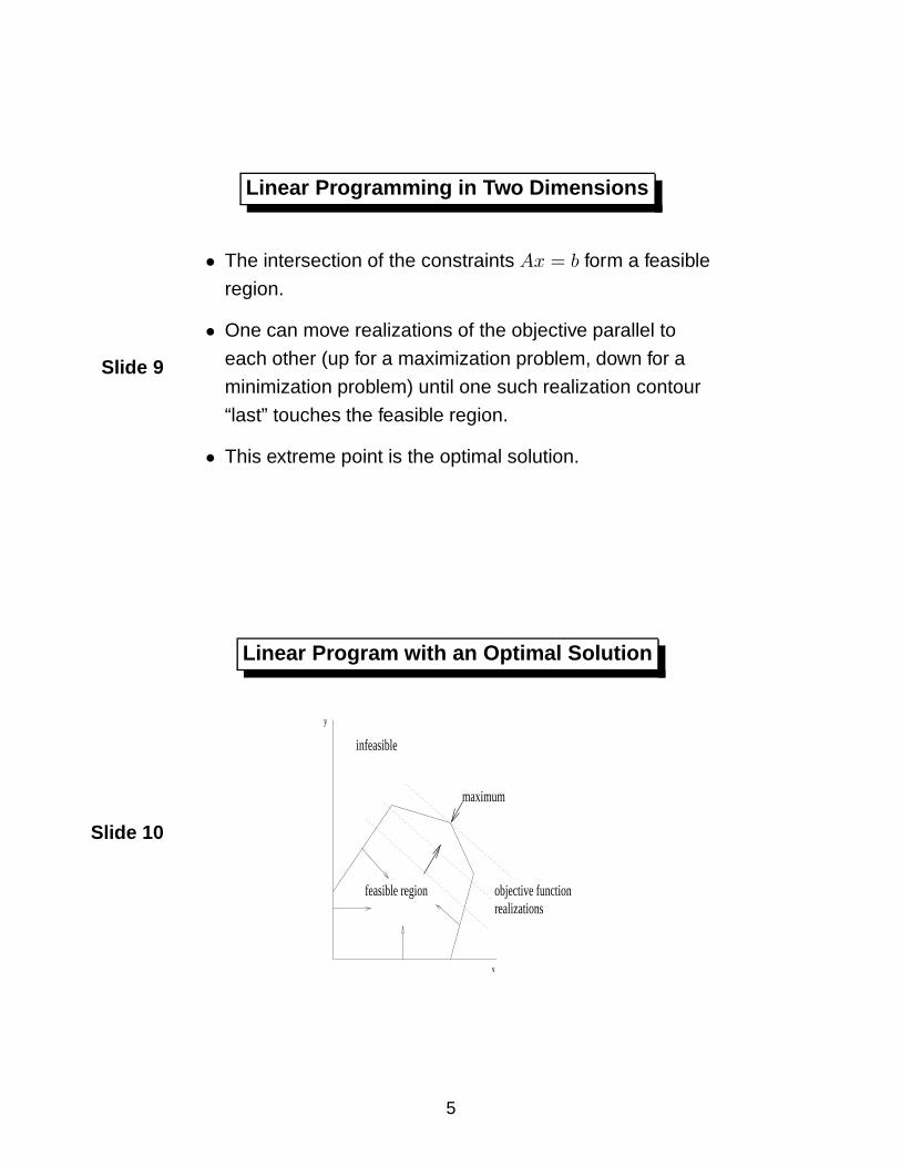
Slide 9
Linear Programming in Two Dimensions
• The intersection of the constraints Ax = b form a feasible
region.
• One can move realizations of the objective parallel to
each other (up for a maximization problem, down for a
minimization problem) until one such realization contour
“last” touches the feasible region.
• This extreme point is the optimal solution.
Slide 10
Linear Program with an Optimal Solution
x
y
maximum
feasible region objective function realizations
infeasible
5
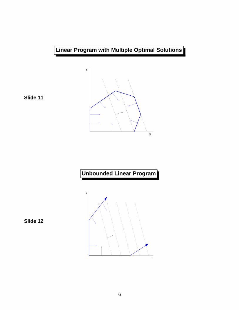
Slide 11
Linear Program with Multiple Optimal Solutions
x
y
Slide 12
Unbounded Linear Program
y
x
6

Slide 13
Infeasible Linear Program
x
y
Slide 14
Two Linear Optimization Algorithms
• Simplex Method: theoretical performance is exponential,
but practical performance is “good” (only check extreme
points, and usually not all of them)
• Interior Point (Barrier) Method: theoretical performance
is polynomial, and practical performance is good for
large-scale problems
7

Slide 15
Simplex Method
x
y
Slide 16
Interior Point Method
x
y
8

Slide 17
Solution 1b: Linear Programming
• Minimum cost: $23.46
– Alloy 1: 0.043
– Alloy 2: 0.283
– Alloy 3: 0.674
Slide 18
Integer Linear Programming
Consider the following system:
(P ) min cy
subject to Ay = b
y ≥ 0 and integer (and binary)
where y is an n× 1 vector of decision variables, and A, c, and
b are known data in the format of an m × n matrix, a 1 × n
row vector, and an m × 1 column vector, respectively.
9

Slide 19
Integer Linear Programming in Mining
• Delineate an ore body, determine an economic envelope
• Schedule “long-term” production, e.g., machine
placements
• Make decisions with logical, e.g., precedence,
constraints: open pit block sequencing, mining strata
Slide 20
Example 2: Integer Programming
W.R. Gracea strip mines phosphates in strata numbered from
i = 1 at the top to i = n at the deepest level. Each stratum
must be removed before the next can be mined, but only
some of the layers contain enough suitable minerals to justify
processing into the company’s three products: pebble,
concentrate, and flotation feed (j = 1, 2, 3).
aBased on D. Klingman and N. Phillips (1988), “Integer Programmingfor Optimal Phosphate-Mining Strategies,” Journal of the Operational Re-search Society, 9, pp. 805-809.
10

Slide 21
Example 2: Integer Programming
The company can estimate from drill samples the quantity aij
of product j available in each stratum i, the fraction bij of
BPL (a measure of phosphate content) in the part of i
suitable for j, and the corresponding fraction pij of pollutant
chemicals. The company wishes to choose a mining plan
that maximizes the product output while keeping the average
fraction BPL of material processed for each product j at least
bj and the average pollution fraction at most pj . Formulate an
integer linear program model of this mining problem.
Slide 22
Example 2: Integer Programming
Table 2: Quantity, BPL, and pollutant for each product and
stratum
Stratum ai1 ai2 ai3 bi1 bi2 bi3 pi1 pi2 pi3
1 4 2 3 .2 .1 .3 .4 .7 .5
2 1 0 2 .1 0 .2 .2 0 .4
3 0 1 4 0 .2 .4 0 .3 .6
4 2 5 0 .3 .7 0 .4 .8 0
5 3 2 5 .2 .3 .2 .4 .5 .4
Limits .25 .3 .27 .7 .9 .7
11

Slide 23
Solution 2a: Integer Programming
Let xi = 1 if we remove stratum i and 0 otherwiseLet yi = 1 if we process stratum i and 0 otherwise
maxn∑
i=1
3∑
j=1
aijyi
subject to xi ≤ xi−1 ∀ i = 2, ..., n
yi ≤ xi ∀ i = 1, ..., nn∑
i=1
bijaijyi ≥ bj
n∑
i=1
aijyi ∀ j = 1, 2, 3
n∑
i=1
pijaijyi ≤ pj
n∑
i=1
aijyi ∀ j = 1, 2, 3
Slide 24
Integer Linear Programming
x
y
12
Slide 25
Integer Programming Optimization Algorithm
• Now, there are a finite, rather than an infinite, number offeasible solutions.
• So, we could enumerate all the feasible solutions, testthem in the objective function, and choose the best one.
• This would take a long time.
• In fact, even though the conventional algorithm uses“smarter” techniques to reduce enumeration, thealgorithm still has theoretical exponential complexity.
• And, in practice, integer programs require far moresolution time than linear programs of commensurate size.
Slide 26
Solution 2b: Integer Programming
• Maximum product output: 12
– Remove strata 1, 2, 3, and 4
– Process strata 3 and 4
13
Slide 27
Mixed Integer Linear Programming
Consider the following system:
(P ) min cx + dy
subject to Ax + Ey = b
x ≥ 0, y ≥ 0 and integer (and binary)
where x is an n × 1 vector of decision variables, y is an n′ × 1
vector of decision variables, and A, E, c, d and b are known
data in the format of an m × n matrix, an m × n′ matrix, a
1 × n row vector, a 1 × n′ row vector, and an m × 1 column
vector, respectively.
Slide 28
Mixed Integer Linear Programming in Mining
• Scheduling production with sequence and tonnage
decisions
• Supporting development decisions with production
constraints
• Combined resolution production scheduling models
14

Slide 29
Example 3: Mixed Integer Linear Programming
A steel mill has received an order for 25 tons of steel. The
steel must be 5% carbon and 5% molybdenum by weight.
The steel is manufactured by combining three types of metal:
steel ingots, scrap steel, and alloys. Four steel ingots are
available for purchase. The weight (in tons), cost per ton,
carbon, and molybdenum content of each ingot are given in
Table 3. Three types of alloys can be purchased. The cost
per ton and chemical makeup of each alloy are given in Table
4. Steel scrap can be purchased at a cost of $100 per ton.
Slide 30
Example 3: Mixed Integer Linear Programming
Steel scrap contains 3% carbon and 9% molybdenum.
Formulate a mixed integer programming model whose
solution will tell the steel mill how to minimize the cost of
filling their order.
Table 3: Ingot properties
Ingot Weight Cost per Ton ($) Carbon % Molybdenum %
1 5 35 5 3
2 3 33 4 3
3 4 31 5 4
4 6 28 3 4
15
Slide 31
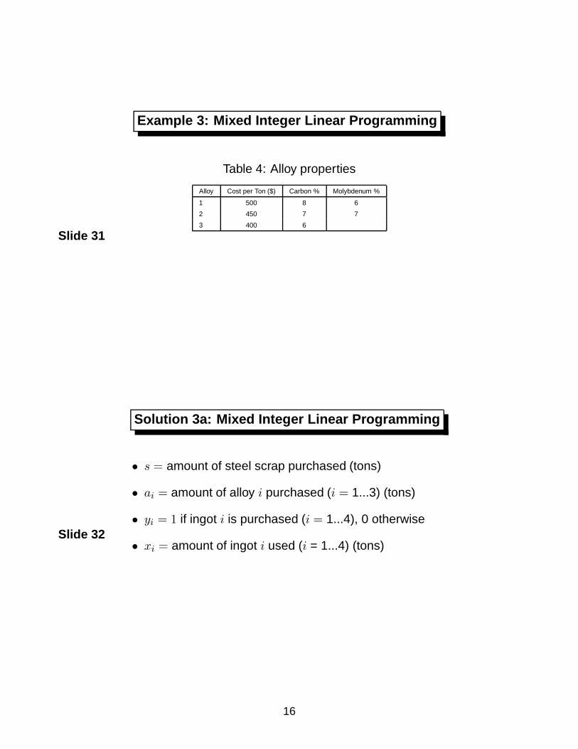
Example 3: Mixed Integer Linear Programming
Table 4: Alloy properties
Alloy Cost per Ton ($) Carbon % Molybdenum %
1 500 8 6
2 450 7 7
3 400 6
Slide 32
Solution 3a: Mixed Integer Linear Programming
• s = amount of steel scrap purchased (tons)
• ai = amount of alloy i purchased (i = 1...3) (tons)
• yi = 1 if ingot i is purchased (i = 1...4), 0 otherwise
• xi = amount of ingot i used (i = 1...4) (tons)
16

Slide 33
Solution 3a: Mixed Integer Linear Programming
min 175y1 + 99y2 + 124y3 + 168y4 + 500a1 + 450a2 + 400a3 + 100s
subject to a1 + a2 + a3 + s + x1 + x2 + x3 + x4 = 25
0.08a1 + 0.07a2 + 0.06a3 + 0.03s + 0.05x1 + 0.04x2 + 0.05x3 + 0.03x4 = 1.25
0.06a1 + 0.07a2 + 0.09s + 0.03x1 + 0.03x2 + 0.04x3 + 0.04x4 = 1.25
x1 ≤ 5y1
x2 ≤ 3y2
x3 ≤ 4y3
x4 ≤ 6y4
s, ai, xi ≥ 0 ∀ i; yi binary ∀ i
Slide 34
Mixed Integer Linear Programming Optimization Algorithm
• These are solved the same way as integer linear
programs are.
17
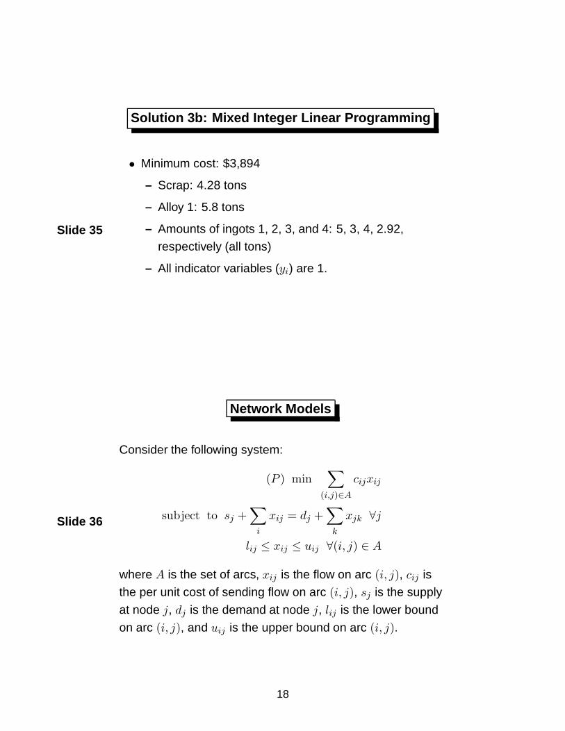
Slide 35
Solution 3b: Mixed Integer Linear Programming
• Minimum cost: $3,894
– Scrap: 4.28 tons
– Alloy 1: 5.8 tons
– Amounts of ingots 1, 2, 3, and 4: 5, 3, 4, 2.92,
respectively (all tons)
– All indicator variables (yi) are 1.
Slide 36
Network Models
Consider the following system:
(P ) min∑
(i,j)∈A
cijxij
subject to sj +∑
i
xij = dj +∑
k
xjk ∀j
lij ≤ xij ≤ uij ∀(i, j) ∈ A
where A is the set of arcs, xij is the flow on arc (i, j), cij is
the per unit cost of sending flow on arc (i, j), sj is the supply
at node j, dj is the demand at node j, lij is the lower bound
on arc (i, j), and uij is the upper bound on arc (i, j).
18

Slide 37
Network Models in Mining
• Assigning equipment to jobs
• Making equipment replacement decisions
• Block sequencing with special structure
• Determining the ultimate pit limits
Slide 38
Benefits of Network Models
• You get integrality for free
• You can solve them very quickly
• You can depict them graphically
19
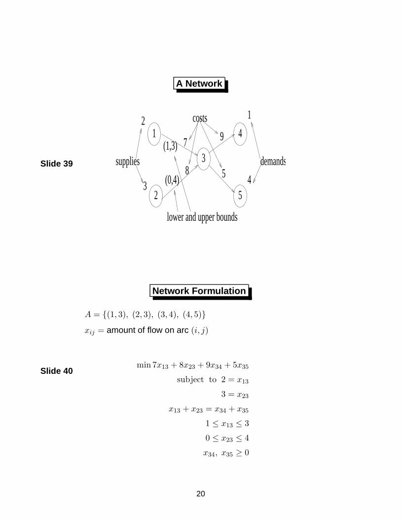
Slide 39
A Network
2
3
1
42
7
8
9
5(0,4)
(1,3)4
5
1
demandssupplies
costs
lower and upper bounds
3
Slide 40
Network Formulation
A = {(1, 3), (2, 3), (3, 4), (4, 5)}
xij = amount of flow on arc (i, j)
min 7x13 + 8x23 + 9x34 + 5x35
subject to 2 = x13
3 = x23
x13 + x23 = x34 + x35
1 ≤ x13 ≤ 3
0 ≤ x23 ≤ 4
x34, x35 ≥ 0
20

Slide 41
Example 4: Network Models
The district manager of the Whiskey Coal Mining Companywants to maximize his profits from his district operations. Thedistrict has two mines and two mills in operation. Productsfrom Mine #1 are shipped to Mills #1 and/or #2; however,Mine #2 ships coal only to Mill #2. Production andtransportation schemes, capacities, and costs are given inTables 5-7 below. Mill #1 yields $4 profit per ton mined, andMill #2 yields $5 profit per ton mined. Please draw acorresponding minimum cost flow graph whose solutionwould maximize profits. Label all supplies, demands, costs,and lower and upper bounds on your directed network, asapplicable. Explain your answer.
Slide 42
Example 4: Network Models
Table 5: Capacity (tons) of and cost of mining at each mine
Mine lower bound on capacity upper bound on capacity mining cost per ton
1 1 6 $2
2 1 7 $2
Table 6: Capacity (tons) of and cost of transporting coal from
mine to mill
Mine Mill lower bound on capacity upper bound on capacity transportation cost per ton
1 1 2 4 $1
1 2 0 5 $2
2 2 2 8 $4
21

Slide 43
Example 4: Network Models
Table 7: Capacity (tons) of each mill
Mill lower bound on capacity upper bound on capacity
1 0 5
2 1 9
Slide 44
Solution 4a: Network Models
2
2
2
1
4
5
4
(1, 6)
(1, 7)
(2, 4)
(0, 5)
(2, 8)
(0, 5)
(1, 9)
S
1
2
1
2
T
Mine Mill
22
Slide 45
Solution 4a: Network Models
Costs of extraction at each mine, and transporting the orefrom the mines to the mills are given on the arcs from thesource to the mines, and from the mines to the mills,respectively. Profits from each mill are given as negativecosts on the arcs terminating at the sink. Lower and upperbounds on capacity at the mines, and between the mines andthe mills are given on the arcs from the source to the mines,and from the mines to the mills, respectively. Capacities atthe mills are given on the arcs terminating at the sink.
An optimal solution to this minimum cost flow problem willyield the optimal distribution plan from the mines through themills.
Slide 46
Solving Network Models
• There are very fast (polynomial time) algorithms to solve
network models.
• Performance gains (over conventional linear
programming solvers) are significant for large models.
• If the model is small or fast solutions are not important,
use a linear programming solver to solve a network
model.
23

Slide 47
Solution 4b: Network Models
• Minimum cost: $4
– Mine 1: Extract 6 tons of coal and send 2 tons to mill
1 and 4 tons to mill 2
– Mine 2: Extract 2 tons of coal and send both to mill 2
– Mill 1: Process and sell 2 tons of coal
– Mill 2: Process and sell 6 tons of coal
Slide 48
Nonlinear Programming
• We will only consider nonlinear programs with
continuous-valued decision variables.
• Generally, nonlinear programming is divided into
constrained and unconstrained nonlinear models.
• Why did we not address unconstrained linear
programming?
• You have seen many unconstrained nonlinear
optimization problems before.
24
Slide 49
Nonlinear Programming in Mining
• Fitting curves to data
• Minimizing quadratic deviation of production output from
target levels (in the short-, medium-, or long-terms)
• Incorporating geotechnical considerations into
production scheduling or other planning models
Slide 50
Example 5: Nonlinear Programming
A mine manager wants to allocate between 10% and 60% of
his available mining capacity to mining each of the precious
metals gold, silver, and copper. With market prices varying
wildly from year to year, he has done some research on past
performance to guide his decisions. Table 8 shows the
average return for each precious metal ($/oz.) and the
covariances among the categories that he has computed.
Formulate a constrained nonlinear program whose solution
would tell the mine manager the least risk plan (using only
covariance terms as a measure of risk) that will average a
return of at least $90.
25

Slide 51
Example 5: Nonlinear Programming
Table 8: Return and covariance matrix for precious metals
Gold Silver Copper
Dollar Return ($/oz.) 77.38 88.38 107.50
Covariance
Gold 1.09 -1.12 -3.15
Silver -1.12 1.52 4.38
Copper -3.15 4.38 12.95
Slide 52
Solution 5a: Nonlinear Programming
Indices:
• i = type of metal in first category, i = 1, 2, 3
• j = type of metal in second category, j = 1, 2, 3
Parameters:
• Ri = average return of metal type i ($/oz) (see table)
• Vij = covariance between metal i and metal j (see table)
• h = minimum return required ($) ($90)
• l = lower bound on capacity (10%)
• u = upper bound on capacity (60%)
26

Slide 53
Solution 5a: Nonlinear Programming
Variables:
• Pi = proportion of capacity devoted to mining metal type i
• P̂i = amount of precious metal i mined (oz.)
Formulation:
min3∑
i=1
3∑
j=1
VijPiPj
Slide 54
Solution 5a: Nonlinear Programming
Formulation:
s.t. li ≤ Pi ≤ ui ∀ i
3∑
i=1
Pi = 1
3∑
i=1
RiP̂i ≥ h
P̂1
P1=
P̂2
P2=
P̂3
P3
P̂i ≥ 0 ∀ i
27

Slide 55
Constrained Nonlinear Optimization Problem
min f(x)
subject to hi(x) = bi ∀i = 1...j
gi(x) ≤ ci ∀i = j + 1, ...,m
Slide 56
Difficulties with Nonlinear Optimization
• Functions may not be well behaved.
• Specifically, f may not be convex (or concave).
• A local optimal solution may not be a global optimal
solution.
28

Slide 57
Illustration of an Ill-behaved Nonlinear Function
Slide 58
Convex and Concave Functions
• Certain functional forms for f will ensure that a local
optimal solution is globally optimal.
• Specifically, if f is convex and the sense of the objective
is minimize, then a local optimal solution will be globally
optimal.
• And if f is concave and the sense of the objective is
maximize, then a local optimal solution will be globally
optimal.
29
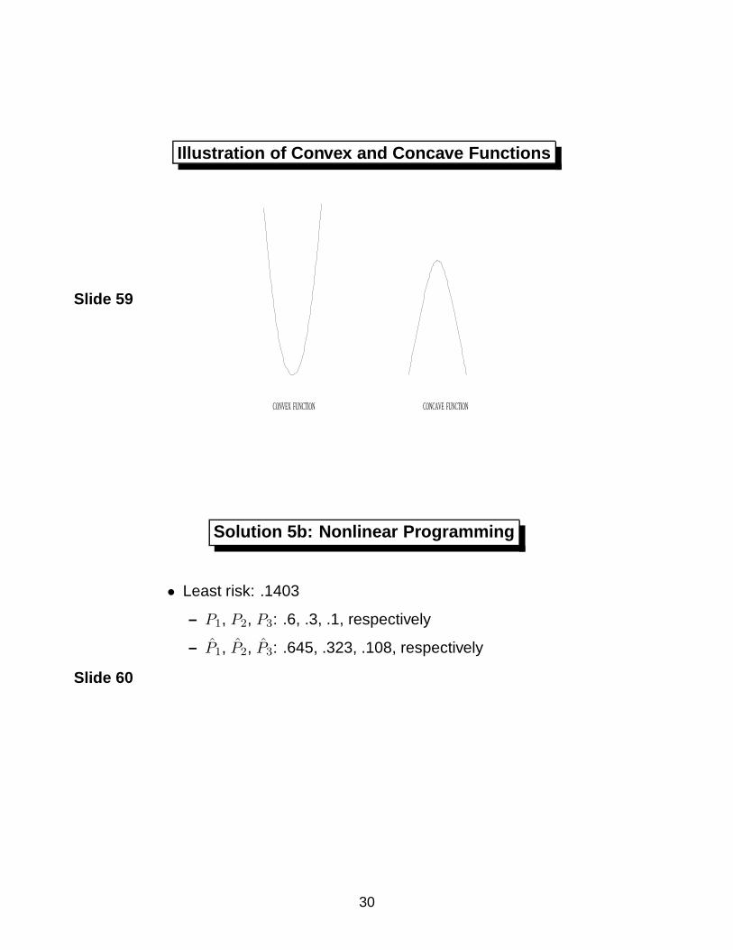
Slide 59
Illustration of Convex and Concave Functions
CONCAVE FUNCTIONCONVEX FUNCTION
Slide 60
Solution 5b: Nonlinear Programming
• Least risk: .1403
– P1, P2, P3: .6, .3, .1, respectively
– P̂1, P̂2, P̂3: .645, .323, .108, respectively
30