Mouse/Rat ECG

Equipment:1. IX-BIO4 or IX-BIO8

2. Needle Electrodes: C-ISO-GNE5 platinum needle electrodes.

3. Computer

4. Optional: C-PB-P1 :Piggy-Back Male/Female Safety Pin Connector to Single Female Safety Pin Connector

5. Optional: Temperature monitoring system.

Supplies:1. Isoflurane inhalation anesthetics

2. Optional: Heat lamp

3. Masking tape

4. Gauze

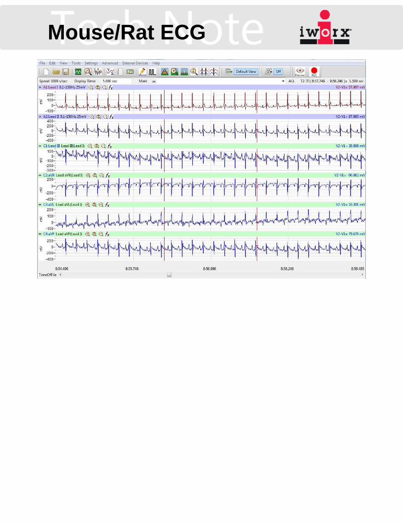
Overview: The Electrocardiogram ( ECG) is recorded and analysed with the iWorx Data acquisition and analysis system. Lead I and Lead II ECG is collected by connecting needle electrodes to the 4 limbs of the animal. Lead II, aVF, aVL, aVR can be calculated by software if needed. For routine screening, Lead II is typically used. The recorded ECG is analysed using the ECG analysis module for LabScribe

Recorder Setup:Place the recorder on the bench close to the computer.

Connect the USB cable to recorder and the computer

Click on the LabScribe shortcut on the computer’s desktop to open the program. Alternately, click on the Windows Start Menu, select All Programs, and then the listing for iWorx. Select LabScribe. The LabScribe Main window will appear once the program opens.

From the Main window, select the Settings tab and then click on “Load Group...”.

Locate the Research Settings folder (default location is: C:Program Files:iWorx:Labscribe:Research Settings...), Open the IX-BIO folder which contains the settings group IXBIO.iwxgrp. Select this group and click Open.

Again, select the Settings tab. Below “Default Setting” is a list of settings, select the Animal Heart menu and then the IX-BIO_SixLeadECG_Rodent settings file from the list.

LabScribe will be configured by the IX-BIO_SixLeadECG_Rodent settings file, and a pdf setup document will open.

Note: if you do not see the Research Settings folder in the LabScribe folder, Reinstall LabScribe, making sure that the Research settings are installed.

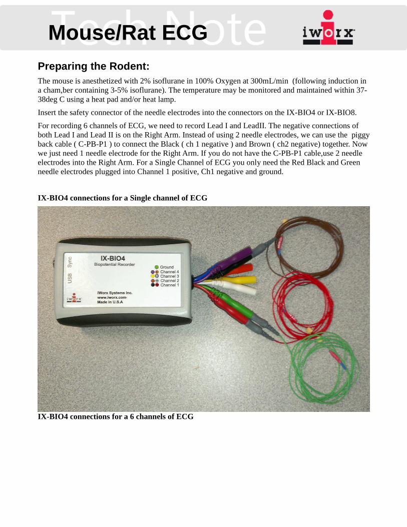
Mouse/Rat ECGPreparing the Rodent:The mouse is anesthetized with 2% isoflurane in 100% Oxygen at 300mL/min (following induction in a cham,ber containing 3-5% isoflurane). The temperature may be monitored and maintained within 37-38deg C using a heat pad and/or heat lamp.

Insert the safety connector of the needle electrodes into the connectors on the IX-BIO4 or IX-BIO8.

For recording 6 channels of ECG, we need to record Lead I and LeadII. The negative connections of both Lead I and Lead II is on the Right Arm. Instead of using 2 needle electrodes, we can use the piggyback cable ( C-PB-P1 ) to connect the Black ( ch 1 negative ) and Brown ( ch2 negative) together. Now we just need 1 needle electrode for the Right Arm. If you do not have the C-PB-P1 cable,use 2 needle electrodes into the Right Arm. For a Single Channel of ECG you only need the Red Black and Green needle electrodes plugged into Channel 1 positive, Ch1 negative and ground.

IX-BIO4 connections for a Single channel of ECG

IX-BIO4 connections for a 6 channels of ECG

Mouse/Rat ECG

IX-BIO8 connections for a Single channel of ECG

Mouse/Rat ECGIX-BIO8 connections for a 6 channels of ECG

As follows:

Insert the Needle electrodes subcutaneously into the Limbs of the mouse as follows.

• The needle electrode plugged into Ch1 Positive is inserted into the Left Arm of the mouse/rat

• The needle electrode plugged into Ch1 & Ch2 Negative is inserted into the Right Arm of the mouse/rat

• The needle electrode plugged into Ch2 Positive is inserted into the Left Leg of the mouse/rat

• The needle electrode plugged into Ground is inserted into the Right Leg of the mouse/rat

Make sure that the needle only penetrates the skin of the animal and is not into the muscle.

Mouse/Rat ECG

Recording with LabScribe:1. Initiate recording by pressing the red icon labeled “REC”. The icon will now change to black

and be labeled “STOP”.

2. Within 3-5 seconds, the mean signal recording should become centered at midscale by the High-Pass-Filter, and the Auto-Scale button may be used to zoom in on the Y-Axis. The signal may fluctuate for the first few minutes and then stabilize. If there are concerns about the qualityof the data being captured, corrective steps can be taken.

3. When the recording is finshed Click the “STOP” icon.

Mouse/Rat ECG

Mouse/Rat ECGAnalysis

Typical Use:The first step required to use the ECG Analysis Module begins in the Main-Window , and depends upon the range of data that requires analysis. Ensure the ECG signal is not inverted, as viewed in the Main Window—inverted ECG will not work in the module because the R-Waves are assumed the mostpositive points of inflection when parsing data. If the Complete-File or Current-Block is intended foranalysis, the cursors are used to select a section of data containing several good representative ECG cycles, all on a relatively flat baseline—and, no obvious “ugly” data. Alternately, the data range intended for analysis can consist of the Selection between the cursors.

If the initial selection does not work, cursors are provided within the ECG Analysis Module allowing the “template” (and range for Selection) to be redefined from that window. Software places marks on the R-Wave peaks within the selected data on the Input-Data-Graph to convey how it defines the ECG cycles between the cursors.

Once the Main-Window data/threshold selection is complete, from the “Advanced” tab, hover over the“ECG Analysis->” and select “Offline Calculations”. This will open the ECG Analysis Module, in aseparate window, in front of the Labscibe Main-Window.

Ensure the data range and selection on the Channels tab reflect the desired source data and range. From the Settings tab, load the Zebrafish settings from the Load Presets drop-menu. Click Calculate.The program will analyze the selected Data Range, parsing individual sequential Cycles into Groups.

Illustration 1: ECG Analysis Module

Mouse/Rat ECGThe results for each Group are shown in rows of the Output-Data-Table. The Group ECG waveforms are displayed in the Module-Graph. Results of Output-Data-Table the and the Module-Graph can be exported for documentation.

Advanced Use:When pressing Calculate, the module analyzes the selected data range recorded in a Main-Window channel by applying parameters to an algorithm, and parsing the data into chunks—in essence, converting a 'chart' style recording, into multiple 'scope' style snap-shots. Each snap-shot represents an ECG cycle candidate, based upon the algorithm detection parameters in the Settings tab. These candidates are then further sorted by applying parameters in the Artifact Removal tab to discriminate between Good and Bad candidates. Good cycles are used to form Groups, each of which generates an Average ECG cycle, displayed on the Module-Graph, and included in the Output-Data-Table. If the settings cause a large number of cycles to be parsed incorrectly, the settings themselves should be adjusted. Probing the Group and Cycles In Group

Definitions:The ECG Analysis Module consists of an Input-Data-Graph , five Configuration -Tabs (Channels, Settings, Artifact Removal, Detection Algorithms, and Outliers), a Group column, a Cycles In Group column, an output Module-Graph, a Calculate button, and an Output-Data-Table.

Input-Data-Graph:

The Input-Data-Graph is located at the top of the ECG Analysis Module. It shows the data selectionfrom the Main-Window that is used to define the characteristic QRS shape. Software marks the peaks of the R-Waves to indicate how it will parse data. Movable Blue cursors are provided that allow the selection to be modified from within the module. Ideally, several complete ECG cycles that are representative of the data set for analysis should be encompassed by the cursors.

The data set between the cursors is significant because the ECG Analysis Module uses this as a template to characterize the typical ECG cycle within the data of interest, which is then used to “tune” the algorithm so that it is best able to detect all available ECG cycle candidates. If, for example, the typical P-Wave amplitude is 0.2mV, and the typical R-Wave amplitude is 1mV, the threshold used to detect the R-Waves must be set high enough so that P-Waves are rejected, but not the R-Waves. If selected data between the cursors also included a 20mV “spike” due to movement, the threshold for theR-Wave will be elevated such that it may preclude detecting the actual ECG R-Waves—rejecting them as too small, much as would happen when discriminating between R and P-Waves in normal conditions.

Channels Tab:

The Channels Tab allows selection of the scope and source of the data to be analyzed. These are accessed via drop-down menus:

1. “ECG Channel” selects the ECG channel that contains the data set to be analyzed. The default is the raw ECG channel, “A1”, but can select a filtered or computed channel.

2. “Data Range”, allows you to analyze data from the “Selected”, “Current Block”, or “Complete File”. Selected includes the data recorded between the two cursors in the Main-

Mouse/Rat ECGwindow. Current Block includes the data recorded in the entire data block where the cursors were placed in the Main-window. Complete File includes the data recorded in the entire file in the Main-window.

Settings Tab:

The Settings Tab allows adjustment of parameters that tune how the algorithm of the ECG Analysis Module detects the characteristic points in the selected ECG cycles. The Mouse Presets will configurethese parameters for you, though they may be modified as desired. Once selected, the Mouse Presets will remain until a different choice is loaded—even if software is closed and reopened. These parameters are accessed via drop-down menus and Up/Down arrows allowing multiple options to enter new values:

1. “Average” specifies the amount of data to be used when constructing Groups. By default, the number of Good cycles is used to specify this amount.

Alternately, the amount of data per Group can be defined as a period of time, in Seconds. This is not recommended for normal use because fixing time allows for Groups within a recording to contain different numbers of cycles—because the cycle period varies—and thus, when comparing the tabulated output-data, the resultant data can be skewed, depending on the number of cycles actually included when averaging the data. The ECG Analysis Module doesn't have a minimum Group period, and if the specified period is too small to contain complete ECG cycles, the result may be problematic.

2. “Typical QRS Width” specifies the typical period—in mS—from the centers of the Q to S waves. This aids the algorithm in finding the Q and S-waves after it has identified—and marked—the R-Wave.

3. “Pre-P Baseline” specifies—in addition to the “Maximum P-R” field, the period—in mS—to be graphed, preceding the beginning of the center of the R-wave... This ensures that the graph frames the cycles with adequate data leading up to the P-wave to provide context.

The Module-Graph aligns all cycles—across all Groups created per use—such that the center of the R-Waves are all co-located. This allows scanning through the cycles across all Groups with the Up/Down Arrow-Keys, providing an easy method to observe shifts in timing between the ECG complex constituent components. This setting is potentially confusing, however, because the period between P and R waves is not fixed, and thus, the leftmost data included in the graph cannot be both fixed to a specific period of time before the peak of the P-Wave, while still maintaining the alignment of all R-Waves. Software takes the period defined in this field, in addition to the “Maximum P-R” field. If the default setting leaves the beginning of the P-Wave too close to the left-side of the graph, increase this field until satisfied.

4. “Maximum P-R” specifies the maximum period—in mS—that can exist between the centers ofthe P and R-waves for a particular ECG cycle. Software uses this variable to limit the period before the center of the detected R-Wave to scan for the P-Wave. In instances where the P-Wave is undetectable for an ECG cycle, this precludes software from hunting back to the R-Wave of the preceding ECG cycle, and mislabeling that as the P-Wave for the current cycle.

Software detects the P-Wave in order to mark the beginning (Pb), center (P), and end (Pe) of the P-Wave, and to perform calculations placed in the Output-Data-Table. In instances where software misidentifies these points, the markers can be manually placed where desired, or the

Mouse/Rat ECG“Detection Algorithms” parameters may be adjusted—in either case, the Output-Data-Table will be updated to reflect the changes.

5. “Maximum R-T ” specifies the maximum period—in mS—that can exist between the centers ofthe R and P-Waves for a particular ECG cycle. Software uses this variable to limit the period after the center of the detected R-Wave to scan for the T-Wave. In instances where the T-Wave is undetectable for an ECG cycle, this precludes software from hunting forward to the P-Wave of the subsequent ECG cycle, and mislabeling that as the T-Wave for the current cycle.

Software detects the T-Wave in order to mark the beginning (Tb), center (T), and end (Te) of the T-Wave, and to perform calculations placed in the Output-Data-Table. In instances where software misidentifies these points, the markers can be manually placed where desired, or the “Detection Algorithms” parameters may be adjusted to compensated—in either case, the Output-Data-Table will be updated to reflect the changes.

6. “QTc type” provides a drop menu of options to specify the calculation used to determine the the Q and T-Waves interval. Calculation options currently include: Bazett, Fridericia, Framingham, and Hodge.

7. “Measure ST Elevation At” specifies the period—in mS—from the center of the R-wave, at which to measure the ST elevation, relative to zero line. This value is placed in the Output-Data-Table.

8. “Isoelectric Line is” provides a drop menu of options to specify the method used to calculate the Isoelectric Line. Calculation options currently include: Mean Of All Points, Mean Of Pre-PPoints, and Zero. The Isoelectric Line is displayed on the Module-Graph as a green line.

9. “P Wave May Be Larger Than R Wave” provides a check-box which, conveys to software that for the current ECG analysis, the P-Waves are of larger amplitude than the R-Waves. By default software assumes that R-waves are the largest amplitude components of the ECG complex, and then uses this when parsing data. If this option was not included, in these instances, software would misidentify a P-Wave as an R-Wave, which would then corrupt the procedures for detecting the P and T-Waves.

10. “Inverted T-wave” provides a check-box which when selected, alerts software that for the current ECG analysis, the T-waves are inverted. Software then looks for a local minimum—instead of maximum—point of inflection when identifying the T-Wave.

11. “Ignore First ___ Seconds In Block” specifies—in Seconds—a period of data to ignore at the beginning of the selected data block. This is useful where the beginning of the collected data includes poor data, for example, where the electrodes were being adjusted for optimal placement.

12. “Cycle Detection Threshold Sensitivity” provides a mechanism to tune how software detects R-Waves. Increasing the value in this field, will make software accept more possible ECG R-Waves as valid. Lowering the value will make it more selective.

The characteristic QRS complex is determined by the data selection between the cursors when importing data for analysis—or modified after entering the ECG Analysis Module. The value in this field provides software with a number to divide the R-Wave amplitude of the characteristic QRS complex in order to set a threshold value to use for detecting R-Waves. By default, the value in the field is set at 3, which means that the threshold is set at 1/3rd the

Mouse/Rat ECGamplitude of the R-Wave in the characteristic QRS complex. Only data that exceeds that threshold is considered a possible R-Wave. This ensures that other points of inflection such as P-Waves are not miss-characterized as R-Waves. By contrast, increasing the value in the field to 6 would set the threshold at 1/6th the amplitude of the R-Wave in the characteristic QRS complex, which allows more data to be considered as possible R-Waves.

Artifact Removal Tab:

The Artifact Removal Tab allows adjustment of parameters that tune how the algorithm of the ECG Analysis Module rejects possible ECG cycles. Effectively, this tab provides multiple discriminators, any of which can cause rejection of a cycle candidate. The Mouse Presets will configure these parameters for you, though they may be modified as desired. Once selected, the Presets will remain until a different choice is loaded—even if software is closed and reopened. These parameters are accessed via drop-down menus and Up/Down arrows allowing multiple options to enter new values:

1. “Rate” specifies—in Beats/Minute—the window of frequencies that are allowed. Cycle candidates that have exceeded the Cycle Detection Threshold Sensitivity, will be excluded if they occur too rapidly—or if they occur with too infrequently.

Note that for example, this implies that if a recording were to “flat line” for significant periods of time around an isolated ECG cycle that matched the characteristic QRS complex exactly, thatcycle would be rejected if the specified Rate envelope was set above zero.

2. “R Amplitude” specifies—in the units data was imported in—the window of R-Wave amplitudes (relative to the isoelectic-line) that are allowed. This discriminator is used to ensure that the included R-Waves are consistent with the characteristic QRS template. If the ECG cycles amplitudes are typically 1mV, this field could be set to reject R-waves greater than 5mV for example. This precludes any R-Wave candidate outside this window to be rejected.

3. “Activity ” specifies— in the units data was imported in—the allowable cumulative deviation between adjacent data points across the ECG cycle. Specifically, the sum of the absolute-valuesof the difference between each data sample and the preceding data sample is calculated across the samples within the cycle. If this value exceeds the value specified in the Activity field, that cycle will be rejected.

ActivityCalculated = Σ (ABS(SampleN – SampleN-1)), across all samples in cycle.

Note that the calculated Activity can exceed the defined threshold either by including a large number of small shifts, or a small number of larger shifts, or some combination of the two. Further, the defined value requires a proportional relationship to the characteristic QRS template. If the typical R-Wave amplitude is 1mV, the allowable Activity should be five times larger than for a 5mV R-Wave simply because the allowable sample to sample deviations for an ideal recording will increase by that factor.

4. “Noise” specifies—in the units data was imported in squared—the allowable amount of Standard Deviation. This is useful for removing data that has been modulated by 60Hz noise—or other relatively slow modulations that are too slow to be caught by the Activity setting.

NoiseCalculated = Σ (ABS(SampleN – Isoelectic-Line)2), across all samples in cycle.

A Minimum to Maximum range of Noise is specified. By default, the Minimum is 0, because as a rule, this is used to discriminate against noisy signals so that clean signals can be averaged

Mouse/Rat ECGand interpreted. However, by providing a minimum setting, the tool can also discriminate to only view signals with a minimum level of noise in case one wanted to sort those to correlate them to some activity, for example.

5. “Minimum ” specifies—in the units data was imported in—a window of amplitude that the minimum amplitude contained in the ECG cycle analyzed must reside within. This acceptable envelope is defined with respect to the isoelectric-line.

Illustration#3 depicts how the Minimum artifact rejection tool defines a window that the minimum amplitude in the cycle is required to sit within. It also depicts how the R Amplitude artifact rejection tool defines a window that the R-Wave peak minus the isoelectric-line must sit within.

Detection Algorithms Tab:

The Detection Algorithms tab defines how the algorithms determines—and marks—the following parameters:

1. Beginning Of P-Wave: Software defines a value equal to the Isoelectric-Line plus a signed percentage of the peak P-Wave value—defined in this field—and searches to the left of the peakof the P-Wave for this value, and marks that location with a Pb marker.

2. End Of P-Wave: Software defines a value equal to the Isoelectric-Line plus a signed percentage of the peak P-Wave value—defined in this field—and searches to the right of the peak of the P-Wave for this value, and marks that location with a Pe marker.

3. Beginning Of Q-Wave: Software defines a value equal to the Isoelectric-Line plus a signed percentage of the peak R-Wave value—defined in this field—and searches to the left of the peak of the R-Wave for this value. This field provides a drop-menu allowing a software to either align with the negative crossing (moving from peak of R-Wave backward in time toward the Q-Wave) or the positive crossing (moving from peak of Q-Wave backward in time toward

Illustration 2: R Amplitude And Minimum Artifact Removal

Cycle-Minimum

R Amplitude(min.)

Minimum (min.)

Minimum (max.)

R Amplitude(Max.)

Cycle Measure R-Amplitude

Mouse/Rat ECGthe P-Wave). Ideally, the Q-Wave is a small amplitude negative excursion from the isoelectric-line, shortly after the end of the P-Wave, and the selection provided in this fields drop-menu allows the Qb marker to be placed on either the falling or rising edge of that excursion.

4. End Of S-Wave: Software defines a value equal to the Isoelectric-Line plus a signed percentage of the peak R-Wave value—defined in this field—and searches to the right of the peak of the R-Wave for this value. This field provides a drop-menu allowing a software to either align with the negative crossing (moving from peak of R-Wave forward in time toward the S-Wave) or the positive crossing (moving from peak of S-Wave forward in time toward the T-Wave). Ideally, the S-Wave is a small amplitude negative excursion from the isoelectric-line, immediately following the end of the R-Wave, and the selection provided in this fields drop-menu allows the Se marker to be placed on either the falling or rising edge of that excursion.

5. Beginning Of T-Wave: Software defines a value equal to the Isoelectric-Line plus a signed percentage of the peak T-Wave value—defined in this field—and searches to the left of the peakof the T-Wave for this value. The Tb marker is placed in this location.

6. End Of T-Wave: Software defines a value equal to the Isoelectric-Line plus a signed percentage of the peak T-Wave value—defined in this field—and searches to the right of the peak of the T-Wave for this value. The Te marker is placed in this location.

Outliers Tab:

The Outliers tab provides a report of the cycles—labeled by Block number and Cycle-Count—rejectedby software. Cycles manually included after software rejects them are also noted in a separate list. Thislisting allows online investigation of the cycles, and is included in the final export.

Group:

The number of cycles to Average specified in the Settings tab defines the number of Good cycles to include in each Group. Any Bad Cycles encountered when sequentially parsing the data are included,but are “disabled” by default.

There are two cases where a Group may contain less cycles than specified: 1) The final Group will be incomplete, where inadequate cycles are available to complete it, or 2) The end of a Block is encountered while constructing a Group. A Group cannot include cycles spanning multiple Blocks of data because the Block typically demarcates the periods of data acquisition before and after a drug is administered that may impact the form of the ECG over time, and it introduces false results when including data from both Blocks when averaging the number of cycles within one Group.

A check-box is provided for each Group. When “checked”, the Group data is included for calculations displayed in the Output-Data-Table. Clicking on the Group-Number will display the Good cycles within that Group in the Module-Graph—regardless of the state of the check-box for that Group.

Cycles In Group:

The Cycles within a Group are labeled by Block# and Cycle-Count. The list reflects the indexed cycles—Good and Bad—that the Module processed to detect the specified number of Good cycles required in the Group. Group#1 will thus always begin with Block#1:Cycle #1, which if Good, will be enabled, and if Bad, will be disabled. It will then include the subsequent cycles processed until the specified number is completed. Clicking on Group #2 then begins with the next available cycle—

Mouse/Rat ECGagain, Good or Bad. Cycles deemed Bad by software can be examined, and checked as Good manually, where an exception is required.

Module-Graph:

The Module-Graph is located at the center-right side of the ECG Analysis Module. It can be used to display the ECG cycles within a Group, including the Group Average ECG cycle. In this mode, the isoelectric-line is displayed in Green, and the Group Average ECG cycle in Red. The current cycle isdepicted in Black, and the the remaining Good cycles are in depicted in Gray.

Alternately, it allows XY graphing of parameters (Rate, R Amplitude, Activity, Noise, and Minimum )from within the Artifact Removal tab. This allows cycles to be sorted—graphically, as dots representing each cycle—by these parameters. Note that software does not preclude graphing any parameter against itself, in which case, the result is always a line. XY graphing is generally useful in separating clusters of similar ECG cycles. It is also useful for graphically identifying how well the Artifact Removal parameters are set for the recording. Toward that end, a Blue adjustable selection rectangle is provided allowing the X and Y parameter minimum and maximum values to be altered by dragging the sides of this selection rectangle. Note that the fields in the Artifact Removal tab will be updated from the Module-Graph. This is depicted in Illustration#4. Note that each dot is color coded,with Good cycles colored Green, rejected cycles colored Red, and the selected cycle colored Blue. Double clicking on any dot selects it. The selected cycle's Group is highlighted, as is the index of the cycle within the Cycles-In-Group column. Similarly, clicking on any Group causes the first contained cycle to be selected, and its dot will be colored Blue on the Module-Graph. Clicking on any particular cycle from the Cycles-In-Group column will select that cycle, and turn the corresponding dot Blue.

The Module-Graph drop-menu allows the following funtionality:

1. Copy-Graph: Copies the graphical content of the Module-Graph to the clip-board.

2. View ECG Graph: Cause the Module-Graph to display the time-domain ECG cycles.

3. View Average ECG Graph: Causes the Module-Graph to only display the Group Average ECG cycle.

4. View Artifact Graph : Causes the Module-Graph to display the XY Artifact Removal parameter selected in the Artifact Removal tab.

5. Export Average Data: Allows exporting the selected Group's Average ECG cycle as a Comma Separated Value text file.

6. Set X Axis Scale: Allows explicit definition of the graph's X-axis scale.

7. Set Y Axis Scale: Allows explicit definition of the graph's Y-axis scale.

8. Auto-Scale The X Axis Scale: forces software to define the graph's X-axis scale to include all cycles.

9. Auto-Scale The Y Axis Scale: forces software to define the graph's Y-axis scale to include all cycles.

Note that the X and Y Scales can alternately be adjusted by right-clicking on the graph, or by dragging the X or Y scale on the screen.

Mouse/Rat ECGAs an example of cycle sorting, consider a hypothetical instance where a recording is made spanning two blocks, the first containing ECG of a fish before dosing it with a drug, and the second block after the drug has affected the fish. Assume that drug causes the typical R-Amplitude to halve. Graphing R-Amplitude Versus Rate will show two clusters representing the Good cycles, one centered around the initial R-Amplitude, the second clustered around the halved R-Amplitude. It is now possible to select one or other cluster using the provided interface, and then to perform Calculate with the updated configuration—effectively only showing those cycles once the Module-Graph is returned to display ECG.

Similarly, if a recording was generally clean, but had areas contaminated by 60Hz noise, those sections might be sorted out by plotting Noise versus Rate.

In Illustration#4, Minimum versus Rate is graphed. The Red dots to the left of the selection interface are rejected because their Rate is insufficient. Those to the right are rejected because the rate is too great. The dots within the selection box are colored Green and are largely clustered between 0 and 8—indicating that the lowest amplitudes in those cycles had a value in that range. There are two Green dots at approximately 30 and 32 which likely should be excluded because their lowest amplitudes are well above the isoelectric-line. Illustration#5 shows that the maximum allowable value for the Minimum discriminator has been lowered to approximately10 via the graphical interface. Note that thetext entry field on the Artifact Removal tab now shows 10.0433, reflecting this change. Clicking Calculate again will update the analysis output of the module. ECG can be viewed again in the Module-Graph by selecting that from the graph's drop-menu. Note that in Illustration#5, the selected Blue dot corresponds to Group#19, Cycle-Index B1:242. Illustration#6 shows that particular cycle in the time domain which shows that it is in fact not a valid ECG cycle, and thus should be rejected. The other dot that was formerly included is Group#15, Cycle-Index B1:160, and it is shown in Illustration#7, and again, it is clearly not a valid ECG cycle.

Illustration 3: XY Graphing

Illustration 4: Modified XY GraphIllustration 5: 1st Cycle Rejected By Minimum Discriminator.Illustration 6: 2nd Cycle Rejected By Minimum Discriminator.

Mouse/Rat ECGOutput-Data-Table:

The Output-Data-Table is located at the bottom of the ECG Analysis Module. It is populated by the analysis results after the Calculate button is pressed. Each row number represents the Group index. The columns contain the calculation results. Manually adjusting the markers (Pb, P, Pe, Qb, R, Se, Tb, T, and Te) changes the calculations without pressing the Calculate button. If, however, the detection or rejection parameters require adjustment, the Calculate button must be pressed to update the Output-Data-Table.

The following buttons are provided as part of the Output-Data-Table:

1. Copy: Copies the text content of the Output-Data-Table to the clip-board.

2. Export : Exports the text content of the Output-Data-Table to a file.

3. Algorithms : Opens a window containing definitions for the various columns, containing calculation results.

4. Table Options: Allows the included calculations for the Output-Data-Table to be customized.It also allows the Time in the calculations to be relative to the Selection-Start, or to the Time-Of-Day.

5. Load Template: Allows the configuration parameter settings to be uploaded from a saved file.

6. Save Template: Allows the configuration parameter settings to be saved to a file.

7. Synch: Provides a mechanism to locate a Group within the Main-Window. The selected Group when the Synch button is pressed will be displayed in the Main-Window. The result will not be seen if the ECG Analysis Module window is maximized in front of the Main-Window.

Recognizing Issues And Optimizing ECG Recording:Good connections to an adequately anesthetized mouse will provide good ECG signal recordings .

The main source of noise is Main pickup. The best way to reduce this is to braid or twist the electrodescables together so that they will pick up the same amount of noise. The amplifier is then able to cancel out the noise that is picked up by the electrodes.

Insufficient Anesthesia, may cause the EMG from the animal to be picked up.