WORKING PAPER

3/2004

IVARS TILLERS MONEY DEMAND IN LATVIA

IVARS TILLERS MONEY DEMAND IN LATVIA

RIGA 2004

© Latvijas Banka, 2004

Computer graphics by Olafs Muiþnieks have been used on the cover.The source is to be indicated when reproduced.

ISBN 9984–676–13–7

The views expressed in this publication are those of the author, senior econometrist of the Bank of LatviaMonetary Policy Department. The author assumes responsibility for any errors and omissions.

ABSTRACT

The econometric analysis of the demand for broad money in Latvia suggests a stablerelationship of money demand. The analysis of parameter exogeneity indicates that theequilibrium adjustment is driven solely by the changes in the amount of money. The demandfor money in Latvia is characterised by relatively high income elasticity typical for theeconomy in a monetary expansion phase. Due to stability, close fit of the money demandfunction and rapid equilibrium adjustment, broad money aggregates can be used as indicatorsof the economic activity.

Key words: money demand, co-integration, exogeneity, vector error correction

JEL classification codes: C22, C32, E41

CONTENTS

Introduction 4

1. Theories of the Demand for Money 61.1 The quantity theory of money 61.1.1 The Fisher quantity theory of money 61.1.2 The demand for money: analysis by Cambridge economists 71.2 The Keynes liquidity preference theory 81.3 The Tobin model 91.4 The Baumol–Tobin money demand model 91.5 The Friedman modern quantity theory of money 10

2. Empirical Models of Money Demand 122.1 The partial adjustment model 122.2 The buffer stock model 142.3 The error-correction model 15

3. The Demand for Money: Problem Investigation in Other Countries 16

4. Modelling Money Demand for Latvia 194.1 Selection of model variables 194.2 Co-integration analysis 204.3 Money demand models in Latvia 22

Conclusions 29

Appendix 1 31

Appendix 2 32

Bibliography 34

3

4

INTRODUCTION

The main objective of the Bank of Latvia is to maintain price stability. In pursuit ofthis objective, the Bank of Latvia has set external stability of the national currency asan intermediate policy goal and is implementing a fixed exchange rate system in Latvia.Under a maturing financial system and deepening monetisation of the economy, theBank of Latvia's policy aimed at regulating bank liquidity to minimise interest ratefluctuations on the money market is constantly gaining in importance. Studies dedicatedto the demand for money are relevant for the monetary policy decision-making process.

Interest rates on the financial market are determined by the interrelation betweendemand and supply. The supply of money is not constant and changes with the Bankof Latvia intervening in the foreign exchange market and employing monetaryinstruments. In recent years, the Bank of Latvia has played an active part in theformation of the money supply. If in the 1990s interventions in the foreign exchangemarket were primary drivers of changes, in 2002 and 2003, with an exception of short-lived periods of buying currency, the growth in the monetary base was affected by theBank of Latvia's foreign exchange swap and repo transactions.

In the country with a small and open economy where no restrictions are set for capitalflows and a fixed exchange rate regime is implemented, the supply of money dependson the demand for it, and the central bank acts under constraints to pursue independentinterest rate targets. A pre-requisite for such a situation is a perfect mobility of capital;however, capital mobility typical for the financial markets of advanced economiesdoes not exist in transition economies. Though the spread between risks related tofinancial instruments in Latvia and the advanced countries is narrowing, the Latvianfinancial market is not yet sufficiently developed and does not have an adequatenumber of liquid financial instruments to become attractive to international short-term investments. Hence, at least in the short run, the correlation between moneymarket interest rates of lats and currencies of the basket to which the lats is pegged isnot close.

In periods when capital flows are not sufficient to achieve interest rate equilibrium,extra volatility of interest rates is possible. With lending playing an ever-increasingrole in the economy, the relationship between money market interest rates and theaggregated domestic demand becomes tighter; hence the significance of liquidityregulatory policy is constantly growing. On the other hand, trade-off is to be foundbetween a more flexible liquidity management policy and stability of the exchangerate peg; this adds to the importance of money demand studies for the purpose ofenhancing stability on the money market in the circumstances of a pegged currency.Moreover, the assessment of stability or instability of the money demand in Latviaand the factors influencing it will be valid also after Latvia joins the Economic andMonetary Union (EMU), as the European Central Bank (ECB), alongside the analysisof general macroeconomic data, places a particular focus on the growth of monetary

5

aggregates that are an important indicator the ECB's monetary policy relies on.

The first two Chapters of the paper are devoted to some major theories related to thedemand for money and methods of their potential empirical application; Chapter 3presents country-specific analysis of the demand for money. The assessment of thedemand for money in Latvia is given in Chapter 4, whereas the concluding part of thepaper contains basic inferences resulting from the study.

6

6

1. THEORIES OF THE DEMAND FOR MONEY

1.1 The quantity theory of money

The economic theory advances a great number of money demand theories that sharea common stance: the major function of money is it being a medium of exchange;hence these theories treat the quantity of money in demand as dependent on thevolume of transactions in the economy. Economists are not unanimous to what extentthe demand for money depends on changes in interest rates, and the analysis of thisissue deserves particular attention in the money theory.

The quantity theory of money was developed in the 19th and early 20th century, and itshows the relationship between the quantity of money in circulation and aggregateincome. This theory provides an explanation how much money will be held at a definitelevel of aggregate income; hence the quantity theory of money is also a theory of thedemand for money. The view that interest rates do not affect the demand for money isan essential feature of this theory.

1.1.1 The Fisher quantity theory of money

American economist I. Fisher ranks among the developers of the classical quantitytheory of money. His theory (14) explains the relation between the quantity of moneyin circulation and the volume of transactions in the economy. As measuring the volumeof transactions is complicated, the Fisher theory has been modified to link the quantityof money with the amount of spending on goods and services produced in the economy.The quantity of money is dependent on both the total amount of spending and theintensity of using money in settlements. In the Fisher theory, this dependence isexpressed by the velocity of money V, which measures the average number of timesper year a unit of money is used to settle up for goods and services:

[1],

whereM is the quantity of money;P is the price level;Y is the output.

The Fisher equation expressing the relation between the quantity ofmoney in circulation and nominal income of the economy is obtained from thedefinition of the money velocity. The Fisher equation, without any additionalassumption on the velocity of money, is an identity – a relation that always holds bydefinition, therefore the Fisher quantity theory of money is based on the analysis offactors affecting the velocity of money.

7

The velocity of money is affected by institutional and technological factors thatdetermine the type of payment (cash, settlement accounts). According to Fisher'sstance, effects of institutional factors change slowly over time, and the velocity ofmoney is relatively constant; hence in the shorter run, the quantity of money dependsonly on the nominal income level. Where the money market is in equilibrium, thequantity of money in the economy is equal to the demanded amount of money Md.Assuming that the velocity of money is constant, the equation of the demand for moneyis obtained from the Fisher equation:

[2],

where the constant k is inversely proportional to the velocity of money. As this theorybuilds on the assumption that money functions only as a medium of exchange and isheld in the amount needed for settlements, the Fisher theory rejects the dependenceof the demand for money on interest rates.

1.1.2 The demand for money: analysis by Cambridge economists

Independently of I. Fisher, Cambridge economists A. Marshall and A. C. Pigoudiscovered an identical relation between money and the volume of transactions.Consistency of the two equations notwithstanding, the analyses conducted by I. Fisherand the Cambridge economists differ noticeably.

First, the theories developed by I. Fisher and the Cambridge economists use distinctiveapproaches to the problem. The focus of the Cambridge quantity theory of money isnot on the analysis of market equilibrium but on the choice of individual economicagents. In contrast to the Fisher theory concerning factors that affect the quantity ofmoney needed for conducting transactions, the Cambridge theory focuses on thequantity of money that economic agents would like to hold under certain circumstances.

Second, in addition to an argument in the Fisher theory that money serves as a mediumof exchange, the Cambridge economists view money also as a store of value; hencethe volume of transactions is a significant yet not the only factor having an impact onthe demand for money. The Cambridge theory deals also with the role of wealth andinterest rates. With wealth of economic agents increasing, the volume of financialassets (including money) held for storing wealth should have grown. Assuming thatwealth, the volume of transactions and the level of income are proportional, the demandfor money is also proportional to the nominal income.

Emphasising the significance of the transaction volume for the formation of the demandfor money, the Cambridge economists treated the coefficient k as constant; however,the values of this coefficient may be subject to short-term fluctuations, as the choiceof economic agents to use money as a store of value will be influenced by interestrates and the expected return on other assets.

8

1.2 The Keynes liquidity preference theory

Until the Great Depression, economists shared the view that in the longer run thevelocity of money is affected by technological changes, and in the shorter run instabilityis not typical for it. Following the notable fall in the velocity of money during theGreat Depression, other determinants of the demand for money were sought to explainvariability of the velocity of money. J. M. Keynes scrapped the view that the velocityof money was constant and developed a theory in which he placed a particular emphasison the role of interest rates. However, his theory not only deals with the factorsinfluencing the money demand but provides also a deeper insight into causes for holdingmoney. Proceeding from the analysis of these causes, J. M. Keynes arrived at threemotives: the transaction, precautionary and speculative motive.

Pointing out that the need for money is determined by its function as a medium ofexchange, the Keynes theory argues that the demand for money basically depends onthe volume of transactions. Assuming that the volume of transactions is proportionalto income, this component of the money demand should also be proportional to income.Acknowledging that money functions as a store of value, J. M. Keynes proposed thatin addition to using money for making planned payments there is a need to use moneyto cover unforeseen expenses. According to J. M. Keynes, the quantity of money heldfor the precautionary motive is mainly affected by the level of planned costs inproportion to the income level. Consequently, this component of the money demandis proportional to income.

J. M. Keynes adopted the stance of the classics of the economic theory that money isa medium of storing value. This function of money gives rise to the so-called speculativemotive for holding money. In addition to the argument about the close relation betweenthe stored wealth and the income level, J. M. Keynes emphasised the importance ofinterest rates for economic agents to make decisions on the amount of money to beallocated for storing wealth. When changes in interest rates are anticipated and whenresulting from such changes the placement of speculative capital does not ensure thelargest possible return, economic agents would act reasonably and move their capitalto such financial assets that yield the largest return. In J. M. Keynes' view, the assetsthat can be used to store wealth are money and bonds.

Regarding the financial assets to be used for storing value, the Keynes theory assumesthat economic agents anticipate a move of interest rates toward some "normal" level.The interest rates that are above such a "normal" level are expected to fall; the returnexpected on current investment in bonds could be a good reason to use bonds, notmoney for storing value. When, in turn, a rise in interest rates is expected, the demandfor money would increase, as due to higher interest rates the former investment inbonds would bring about losses.

The value of money is in its purchasing power; hence the money demand is the demandfor its real value. It follows from J. M. Keynes' analysis that the real demand for money

9

Md/P should be positively related to the real income Y and negatively related to theinterest rate r, with the following general money demand function:

[3],

where signs (+ or –) of respective derivations are showed beneath variables.

The speculative money demand model of the Keynes theory produces two explanationsfor fluctuations in the velocity of money. Using the definition of money velocity andthe Keynes money demand function, it is possible to show that under money marketequilibrium the velocity of money increases due to rising interest rates. The Keynesmodel implies that money demand depends on the normal level of interest rates thatcannot be directly observed. Changes in this level may figure as a second cause forunstable velocity of money.

1.3 The Tobin model

Criticism of J. M. Keynes' analysis of the speculative money demand most often focuseson more straightforward assumptions, as the condition regarding the individual choiceto either place capital in bonds or hold it as monetary assets does not foresee a portfoliodiversification possibility. Eliminating this shortcoming, J. Tobin created a speculativemoney demand model in which, along the expected return on assets, he incorporatedrisk of return on assets as an additional portfolio-formation factor. According to thismodel, economic agents are not willing to assume risk. A constant expected return isa significant feature of monetary assets (J. Tobin considered a case of a zero expectedreturn). Bond prices, in turn, may be subject to fluctuations, the return on themcomprises risk, and a negative return is also possible. Hence risk-averse economicagents may still wish to use monetary assets also for storing value, because in this waythe portfolio volatility would be limited. J. Tobin's analysis shows that portfoliodiversification is possible by involving monetary assets, and hence, despite the zeroreturn, money may serve as a medium for storing value.

1.4 The Baumol–Tobin money demand model

W. Baumol (3) and J. Tobin (31) independently of each other advanced similar moneydemand models, which showed that monetary assets held for conducting transactionsmight be affected by interest rates. This model deals with an economy where twotypes of financial assets are available – monetary assets that do not yield interest, andone other type of interest bearing liquid assets, e.g. bonds that cannot be used forsettlements. Only money can be used in transactions, while bond trading is associatedwith transaction costs. In such circumstances, two types of costs are possible – costsrelated to holding money and a brokerage fee, offsetting the shortage of monetaryassets with the income from trading bonds. Economic agents face the problem how to

10

minimise effects of the lost interest and reduce the amount of brokerage fees. If thetotal value of transactions made in a particular period is Y, the brokerage fee relatedto trading bonds is b and the interest rate is r, the minimisation of total expenses leadsto the amount of money required for transaction purposes:

[4].

1.5 The Friedman modern quantity theory of money

M. Friedman developed a theory in 1956 in which he defined the function of thedemand for money on the basis of the theory of demand for assets.

According to this theory, the demand for monetary assets should be related to resourcesat the disposal of an economic agent, i.e. the total amount of assets and the expectedreturn on alternative-to-money assets in comparison with the return on monetaryassets. The demand for assets is positively related to wealth; hence the same relationexists also between the demand for money and the indicator of permanent wealth, ameasure of accumulated wealth introduced by M. Friedman. Permanent income iscalculated as the present value of the expected average future income, and, in contrastto income, this indicator shows less pronounced short-term volatility.

Next to money, also bonds, shares and goods can be used for storing value. The reasonbehind using other alternative-to-money assets for storing value is the expected returnon such other assets against the expected return on money deposits; hence an increasein return on alternative assets relative to monetary assets would result in a diminishingdemand for money. These considerations lead to an assumption that the function ofthe real demand for money is as follows:

[5],

whereYp is the permanent income;rm is the expected return on monetary assets;rb is the expected return on bonds;re is the expected return on shares;πe is the expected inflation.

By contrast to J. M. Keynes, M. Friedman considered that goods and money aresubstitutes, and his theory does not treat the expected return on money deposits as aconstant variable. With interest rates rising in the economy, banks' income from lendingalso increases; in such circumstances, banks, aiming to attract new funds, push up

11

interest rates on deposits. Competition in the banking sector is the factor driving updeposit interest rates until there is no excess profit. Under the impact of these processes,

the difference is rather stable. Due to it, interest rates are likely to have little

impact on the demand for money.

12

2. EMPIRICAL MODELS OF MONEY DEMAND

Theoretical studies of the demand for money indicate that the demand-formationmechanism is complicated and the money demand function can be derived analyticallyonly for highly straightforward models. Theory, however, ranks prominent in empiricalstudies of the money demand, as it furnishes information on variables, derivationsigns and values of parameters of the demand function that can be used in advancingstatistically verifiable hypotheses and interpreting economically empirical results.

According to theoretical models, the money demand could be determined by the pricelevel P, the volume of transactions T made in the economy, opportunity costs of holdingmoney r, and the interest rate R on money deposit. Expecting a stable long runequilibrium, the demand theory for money postulates the relation of the money demandequilibrium and justifies derivation signs of the function:

[6].

Due to stochastic deviations, the equilibrium, in fact, is never achieved, yet in theevent of a stable equilibrium an adjustment to equilibrium should take place.

The theoretically substantiated function of the demand for money is an equilibriumrelation, yet due to changes in the determinants of money demand, equilibrium wouldbe attained with a certain lag. As a rule, economic modelling uses time series withsuch periodicity of observations that does not allow for assuming the adjustment toequilibrium as proceeding without lags; the time series of economic variables compriseinformation on both structural relations of variables and dynamics. Hence specificationof the model, which is appropriate for forecasting, should take into account alsodynamic properties of variables, and it is important to seek for a correct specificationof both the model structure and dynamics.

2.1 The partial adjustment model

The error-correction model is generally accepted for analysing the demand for money.Early studies of the money demand widely exploited the so-called partial adjustmentmodel advanced by G. C. Chow, which can be considered to be a special case of thesingle equation error-correction model. This model extends the conventional moneydemand model by assuming that the actual amount of money may differ from theequilibrium money demand, yet with time the equilibrium is recovered. Even thoughthe conditions for adjustment to equilibrium incorporated in the partial adjustmentmodel are too specific, and volatility of money demand functions has been oftenobserved in empirical studies, this model underpinned the development of dynamicmodels of the demand for money.

The partial adjustment model for money demand has been developed on the basis of

13

the equilibrium approach to the demand for money. The demand equilibrium modelassumes that any factor changes with an impact on the demand for money areimmediately followed by an action of economic agents aimed at complete adjustmentof money balances to the new equilibrium level. The most widely used formulation ofthe money demand long-run equilibrium relation is as follows:

[7],

wherem*

t is the real demand for money under conditions of equilibrium;yt is the real income;rt is variables representing opportunity costs.

All components of the equation are logarithms of corresponding variables in the periodt.

The partial adjustment model assumes that the adjustment to equilibrium moneymarket is hindered by portfolio adjustment costs, which do not allow for the adjustmentof the actual money stock to the desired level in one period of time. According to thescheme proposed by G. C. Chow, for the purpose of describing the equilibriumadjustment dynamics (9), the difference between the actual and equilibrium stock ofmoney diminishes as showed by the following relation:

[8],

where mt is the actually demanded quantity of money and the partial adjustmentcoefficient . When the long-run money demand equilibrium relation iscombined with the equilibrium adjustment relation, the following equation is ob-tained:

[9],

where coefficients a1 and a2 denote the long-run elasticity of money demand, whereasδa1 and δa2 denote the short run elasticity of money demand.

Until the beginning of the 1970s, the partial adjustment model performed well in thestudies of money demand; however, later its application was associated withinsurmountable problems, instability of demand functions for money and thesubsequent inaccurate forecasts of the money stock in particular. However, theapplication of weighted monetary aggregates in an attempt to avoid volatility of themoney demand, which stemmed also from an inaccurate definition of monetaryaggregates, did not eliminate regular forecast errors of the partial adjustment model.

The partial adjustment model is characterised by an extremely low estimation of theinterest rate short-run elasticity, which on average was one order lower than the

14

estimation of interest rate long-run elasticity. The adequacy of the model specificationbecomes highly questionable also due to the fact that the main explanatory factor isthe lagged monetary variable implying a very long period of adjustment to equilibrium.Critical remarks in the address of this model focus also on the current econometricproblems, among which central are the simultaneity bias of parameter estimates andthe spurious regression problem associated with non-stationarity of time series.

2.2 The buffer stock model

In the 1980s, the buffer stock model was developed as an alternative approach for theestimation of parameters of the demand function for money with the aim to offset thepoor performance of the partial adjustment model. The precautionary motive ofholding money underpinned the development of the buffer stock model to justify theproposed dynamic specification. Transaction costs limit the portfolio adjustmentprocess; hence, due to unexpected inflows of money, surplus cash balances may form.As the buffer stock of money allows for offsetting unexpected outflows and inflows ofmoney, economic agents accept temporary fluctuations of the money stock from theoptimum level m*. In contrast to the partial adjustment model where a short-termmoney supply in the economy is determined mainly by the demand, money supplyunder the buffer stock model is exogenous, and it is the money supply factors – openmarket operations and expansionary lending of the banking system – that primarilyinfluence the money stock.

J. Carr and M. R. Darby created a shock-absorbing model (8), which is one of themost popular buffer stock approaches widely used in empirical studies. Under thismodel, a variable representing a money supply shock is additionally included in thedemand function for money, while the specification of dynamics is equivalent to thepartial adjustment model. The first equation of the model by J. Carr and M. R. Darbyis as follows:

[10],

where (mt – m*t) is the unexpected supply but (mt – pt) is the logarithm of the actual

supply of money. The unexpected supply of money m*t is described by the following

equation:

[11].

Z is the vector of variables with a regular effect on money supply as viewed by theeconomic agents, while g denotes model parameters. Criticism of this model so farhas mainly focused on econometric problems implied by its specification. By includingthe variable mt on both sides of the equation, the residual variable ut and mt cannot beviewed as non-correlated.

15

Even though the buffer stock model is theoretically sound, its quality has not beensufficiently appropriate for empirical research, and the model has been scrapped.The basic failure of the model consists in its equilibrium-adjustment dynamics, whichis more complicated than can be captured by the partial adjustment and buffer stockmodels. Nowadays, the analysis of the demand for money most often rests on theerror-correction model.

2.3 The error-correction model

In empirical money demand studies, the error-correction model has taken its place asthe most appropriate instrument of investigation. This approach combines tworelations – the adjustment to the long-run equilibrium upset by the effects of stochasticfactors (error-correction) and the description of short-run dynamics – in a singleequation. The error-correction model represents a methodological trend accordingto which an appropriate specification of the data dynamic structure plays an essentialpart in economic modelling. Over a longer term, the model should represent structuralrelations of the economy, whereas the specification of the short-run dynamics is derivedfrom the analysis of data. The studies of the equilibrium adjustment dynamics haveshown that the process is more complicated than implied by the partial adjustmentand buffer stock models, and it has determined the failure of the two.

In comparison with the above-described models used in analysing the demand formoney, the error-correction model has a number of advantages, of which the possibilityto avoid spurious statistical inferences when analysing the regression of non-stationaryvariables is the first to be mentioned. In contrast to models with only differentiatedtime series, information on long-run relation among variables is not lost when usingthe error-correction model; moreover, the specification allows for distinguishingbetween the short-run and the long-run effect.

Initially, the error-correction model was a single equation model, yet its evolutionresulted in an extended model of several equations or the so-called vector error-correction (VEC) model. This model respects endogeneity properties of variables,and it is an advantage that often supports building of a stable money demand model.

16

3. THE DEMAND FOR MONEY: PROBLEM INVESTIGATION IN OTHER

COUNTRIES

Since the end of the 1970s, when economists in the US and other advanced countrieswere unable to explain the actual development of money aggregates by means of themoney demand function, they have plunged into extensive studies of the demand formoney. Search for causes of and solutions to volatile money demand deepened theoverall perception of the demand for money and fostered the appearance of newmethods of econometric analysis.

Money demand is a significant subject of research for central banks. In Finland, theresearch by A. Ripatti (28) which investigates the demand for money, the models forthe monetary aggregates M1 and M2 have been created using the specification of thevector auto regression (VAR) model, which, on the basis of test results, can be reducedto a single equation model. The advantage of such a modelling strategy is the possibilityto identify, by statistical methods, exogenous factors and simplify the model structureavoiding initial possibly erroneous assumptions regarding exogeneity of variables.The study discloses exogeneity of interest rates and prices. The findings of the studyare consistent with the inference of the economic theory that in a small and openeconomy with a fixed exchange rate regime interest rate fluctuations in a long-runare not caused by money supply but rather by foreign interest rate developments andcurrency risk.

The research paper developed by S. Hendry at the central bank of Canada (21) isamong the numerous studies of the 1990s using the co-integration analysis method ofS. Johansen. The aim of the analysis is to examine long-term relationships among themonetary aggregate M1, prices, output and interest rates in Canada, questioning theexistence of a stable relation that could be interpreted as a long-run demand for money.Quarterly data (1956–1993) have been used in the estimation of co-integrationrelationships. The VEC model analysis has led to the following finding: if M1 exceedsthe long-run demand, M1 will decline and prices will go up, adjusting to equilibrium.The effect is insignificant in terms of output and interest rates, pointing to weakexogeneity of the given variables. Though the outcomes indicate that the adjustmentto monetary equilibrium is determined by fluctuations in money stock and prices, theexistence of real effects of short-run monetary changes are not ruled out. The parameteranalysis of the short-run dynamics leads to a conclusion that changes in the quantityof money do have an effect on the economy over a shorter horison.

The 1980s was the period, when the majority of world central banks scrapped thestrategy of intermediate monetary targets. The main reason for this change of themonetary policy strategy was the growing instability of the relation among the moneysupply, interest rates, income and prices caused by structural changes of the financialmarkets. The central bank of Germany was among those banks that continued topursue the monetary targeting strategy; hence the demand for money has been

17

extensively examined in this country. D. Gerdesmeier's research (16) is dedicated tocomprehensive studies of the part played by wealth in the German demand for money.

M. Scharnagl's paper (29) provides a detailed discussion of suitability of the monetaryaggregate M3 for monetary policy strategy, building on the P* approach developed byJ. J. Hallmann, R. D. Porter and D. H. Small (18). The study provides a comprehensiveinsight in suitability of the definition of money aggregates, stability of the moneydemand, controllability of the monetary intermediate target and the level of its linkagewith the ultimate goal of monetary policy. When defining monetary aggregates, thequestion whether from the point of view of economic agents financial assets includedin a monetary aggregate belong to the same category of assets (money) is usuallyomitted. The choice of a particular combination of financial assets is determined bypreferences of economic agents that can be described by the utility function. Financialassets m are characterised by the weak separability property in relation to commoditiesc, if arguments of the utility function

[12]

can be sub-grouped and the utility function written as follows:

[13].

Weakly separable groups can be viewed as elementary commodities, for the marginalrate of substitution of elements within one group depends only on the amount ofelements within this particular group. If the weak separability property is inherent ina particular financial asset group, open preferences of economic agents should not becontradictory to GARP – the Generalised Axiom of Revealed Preference. Themonetary aggregate satisfies GARP, if under the inequality:

[14],

the following inequality does not hold:

[15],

where m i, m j are financial assets and p i, p j are their prices. Interpreting i and j as timeindices, H. R. Varian proposed verification of this axiom as a non-parametric test foridentification of the weak separability of the financial asset group (32), in such a wayavoiding problems associated with the selection of a certain utility function. Thoughthe period (1977–1995) selected for the study contains observations that do not meetGARP terms for the monetary aggregate M3, the axiom is not violated in the shortenedselected period (1983–1995). It must be admitted that when selecting components ofa monetary aggregate, reliability of this test should not be overestimated because ofits low power.

18

When selecting the monetary targeting strategy, the stability of the money demandfunction is a decisive precondition to use the monetary aggregate as an intermediatemonetary policy goal. The outcomes of testing stability of the demand for moneyconfirm that the narrow monetary aggregate M1 is not appropriate for an intermediatetarget of monetary policy (16), while the demand function of the monetary aggregateM3 is stable and interest rates may be used as a policy instrument in controlling theamount of money.(4)

When certain unanimity regarding theoretical aspects of the formation of the demandfor money was achieved and given the diminishing confidence in monetary aggregatesas sound intermediate targets of monetary policy, economists started to lose interestin the demand for money. Nevertheless, data quality of the monetary sector's indicatorsand a comparatively small number of variables needed for an adequate modelformulation enhanced the application of the money demand analysis whendemonstrating the practical application of new econometric methods. The researchconducted by S. Johansen and K. Juselius (23), which demonstrates the maximumlikelihood method using models of the demand for money in Denmark and Finland,is ranked among the classical works of economic science.

The analysis of money demand is used for the purpose of demonstrating a newtheoretical approach to defining and testing variable exogeneity concepts. The paperby N. R. Ericsson, D. F. Hendry and G. E. Mizon (13) deals with the concepts ofexogeneity, causality and invariance, reflecting the application of the exogeneityconcept in econometric models with co-integrated variables. The given issues ofeconometric modelling are illustrated using the UK money demand model.

The money demand studies have not lost their importance. As countries with unstablemoney demand are also members of the EMU, issues of the money demand stabilityin the euro area, despite the prominent share of Germany, are still in the focus ofresearch. Investigations conducted (5) confirm stability of the demand for the monetaryaggregate M3, which can be explained by both the part Germany plays in the euroarea and the stabilising effect of pooling monetary aggregates of different EMUcountries.

19

4. MODELLING MONEY DEMAND FOR LATVIA

The modelling of the demand for money in Latvia follows three stages. At the firststage, appropriate variables for the money demand model are selected; estimation oftheir stationarity and co-integration is conducted at the second stage, and, finally,proceeding from several statistical tests the optimum specification of the model isderived.

4.1 Selection of model variables

When engaging in money demand investigations, researchers in Latvia face a majorproblem of economic empirical studies, i.e. the selection of statistically measurableindicators that would be compatible with theoretically presented ones. In the moderneconomy, a great many of liquid financial instruments can perform functions of money,and the demand function for narrow monetary aggregates may be instable. Of lessliquid assets with monetary properties, only the share of time deposits is significantfor the Latvian economy. Given the share of deposits in foreign currencies in totaldeposits (almost 40% in early 2004) and the use of foreign currencies in settlements,broad money M2X incorporating deposits in both lats and foreign currencies is thebest measure of the money supply. As the value of money consists in its purchasingpower and the real demand for money is the object of this study, the real quantity ofmoney computed by dividing the nominal indicator with the consumer price index(CPI) is used to characterise the supply of money. Gross domestic product (GDP) atconstant prices of 2000 has been chosen as the income-representing variable.

An important issue of the money demand studies is opportunity costs of holding money,which stem from different rates of return on money and alternative assets. Governmentbonds, whose liquidity on the secondary market of securities compares well to timedeposits, can be considered the most significant alternative for storing wealth.Nevertheless, due to the relatively low level of wealth and income, private personsmost often prefer bank time deposits; therefore, the yield on government bonds inLatvia is not the best indicator for opportunity costs of holding money.

Attempting to incorporate financial sector indicators in the models, one encountersserious additional problems, of which the major one is heterogeneity of data typicalfor the indicators of Latvia's financial markets even over a short period of time. It isassociated with both the dynamic evolution of the Latvian financial sector and the lowlevel of overall development in the mid-1990s to which the time series used inmacroeconomic studies refer. Hence the possibility to ascribe the results obtained bystatistical methods to the current situation is limited. The length of the financial sectortime series is another problem. Data on the secondary market quotations of thegovernment debt instruments became available in 1999 starting with the conduct ofsuch transactions on the Riga Stock Exchange. Though technically these data permitthe assessment of regression parameters for several factors, opportunity costs of cash

20

deposits, according to the theory, are a weak indicator of the money demand and itseffects cannot be observed over such a short period.

Opportunity costs of holding money are incurred also due to a rise in prices. Theindicator of expected inflation might be a considerably more important source ofopportunity costs of holding money than the yield on financial instruments. The depositinterest rate, in turn, pushes up the demand for money. As the time series of annualinflation and interest rates are relatively tightly correlated, the multicollinearityproblem will emerge and reduce the efficiency of parameter assessment if theseindicators are included as separate variables. Another factor of the empirical moneydemand function is the real interest rate on deposits, which is calculated byapproximately assessing the expected inflation rate in the up-coming year on the basisof the current inflation rate.

In the selected period (1996–2003), money supply was not the key factor affectingprices, while inflation in Latvia was mainly driven by price convergence processes andchanges in administratively regulated prices and tax rates. Therefore, the vector ofendogenous variables does not comprise the price level component, as the latter isaffected by factors not included in the model. The model specification assumes that inthe long run the so-called money illusion is non-existent and, therefore, the real demandfor money does not depend on the price level.

The vector of model variables used in the study, thus, is made up of the real supply ofthe broad money using the consumer price index as deflator: m – p = ln(M2X/CPI),GDP at constant prices of 2000: y = ln(GDP) and the real long-term deposit rate:r = iD – πe (graphic charts of indicators' time series are given in Appendix 1). The firstquarter of 1996 is used as the initial sample period, with macroeconomic indicatorsduring the 1995 banking crisis, when the Latvian economy experienced serious shocksdue to which statistical relationships between indicators were loose, being omitted.

4.2 Co-integration analysis

Though theoretically money demand factors can be reduced to comparatively fewaccurately measurable economic indicators (GDP, CPI and interest rates), the latterreflect economic sectors that are mutually interacting with each other. Single equationerror correction methods developed at the initial stage of co-integration analysis areapplicable only if the involved variables are linked by a single co-integration vector;however, even in such cases unbiased parameter estimates are not always obtainable.The estimation of the money demand parameters using the single equation errorcorrection model is applied if the demand factors can be treated as exogenous. Thevalidity of the single equation error correction model and exogeneity properties of itsexplanatory factors can be investigated on the basis of the general co-integrationanalysis developed by S. Johansen.(22)

21

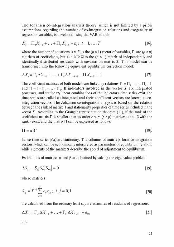
The Johansen co-integration analysis theory, which is not limited by a prioriassumptions regarding the number of co-integration relations and exogeneity ofregression variables, is developed using the VAR model:

[16],

where the number of equations is p, Xt is the (p × 1) vector of variables, Π i are (p × p)

matrices of coefficients, but is the (p × 1) matrix of independently andidentically distributed residuals with covariation matrix Σ. This model can betransformed into the following equivalent equilibrium correction model:

[17].

The coefficient matrices of both models are linked by relations and . If indicators involved in the vector Xt are integratedprocesses, and stationary linear combinations of the indicators' time series exist, thetime series are called co-integrated and their coefficient vectors are known as co-integration vectors. The Johansen co-integration analysis is based on the relationbetween the rank of matrix Π and stationarity properties of time series included in thevector Xt. According to the Granger representation theorem (11), if the rank of thecoefficient matrix Π is smaller than its order r < p, (r × p) matrices α and β with therank r exist, and the matrix Π can be expressed as follows:

[18],

hence time series β'Xt are stationary. The columns of matrix β form co-integrationvectors, which can be economically interpreted as parameters of equilibrium relation,while elements of the matrix α describe the speed of adjustment to equilibrium.

Estimations of matrices α and β are obtained by solving the eigenvalue problem:

[19],

where matrices

[20]

are calculated from the ordinary least square estimates of residuals of regressions:

[21]

and

22

[22].

When solving the matrix eigenvalue problem (see equation [19]), eigenvectors

and eigenvalues are obtained; the eigenvectors

corresponding to the largest values of r are the estimates of co-integration vectors.

For the purpose of determining the number r of co-integration vectors, S. Johansenand K. Juselius developed tests for the rank of the matrix Π.(23) The matrix trace test

is used to check the null hypothesis on the basis of test statistics:

[23],

where are the smallest eigenvalues of p – r. The hypothetical alternative

of this test is the assumption that there are more co-integration vectors than r. Thelargest eigenvalue test appraises the hypothesis H0 : rank(Π) = r – 1 against thealternative rank(Π) = r, using

[24]

as test statistic.

4.3 Money demand models in Latvia

Proceeding from the arguments above, the money demand model is based on theVEC model, which allows for incorporation of information on the dynamic structureof long run interrelation of variables and rather general dynamic structure of datawithout imposing restrictions on exogeneity properties of variables. This approachensures elimination of the spurious regression problem that emerges when using non-stationary time series in the estimation of parameters, and avoidance of simultaneitybias associated with potential endogeneity of variables.

In order to identify the co-integration matrix rank of the VEC model, the Johansentrace test has been applied, with its results summarised in Table 1.

Table 1

RESULTS OF THE CO-INTEGRATION MATRIX TRACE TEST

H0 H1 λ λtrace

α = 0.05 α = 0.01

r = 0* r > 0 0.5139 32.7089 29.7971 35.4582

r = 1 r > 1 0.2242 8.9050 15.4947 19.9371

r = 2 r > 2 0.0159 0.5276 3.8415 6.6349

* The hypothesis is rejected at the significance level of 0.01.

23

The outcomes of the test show that the null hypothesis H0 : r = 0 can be rejected at thecriterion significance level α = 0.05; by contrast, neither the hypothesis H0 : r = 1 northe hypothesis H0 : r = 2 can be rejected. According to these results, the time seriesm – p, y and r are linked by the same co-integration vector, and it can be interpreted asthe demand for money.

The optimum short run specification of the VAR model dynamics has been selectedfollowing AIC information criteria of H. Akaike and SC information criteria ofG. Schwartz, which convincingly confirm that one quarter is the optimum period oflag (see Table 2).

Table 2

VALUES OF LAG LENGTH SELECTION CRITERIA

Q1 Q2 Q3 Q4

AIC –4.5127 –4.2761 –3.9133 –3.5406

SC –3.6883 –3.0394 –2.2643 –1.4590

Table 3

RESULTS OF EXOGENEITY TEST

H0 : γ2 = 0 H0 : γ3 = 0 H0 : γ2 = γ3 = 0

W = 0.060 W = 0.005 W = 0.065

χ20.95

(1) = 3.841 χ20.95

(1) = 3.841 χ20.95

(1) = 5.991

Weak exogeneity of variables in the VEC model can be verified using the coefficientrestriction test of the adjustment-to-equilibrium velocity. Testing exogeneity of GDPand interest rates against co-integration vector parameters, statistics of the coefficientrestriction test and the results of testing critical values of the null hypothesis are givenin Table 3.

The results of testing the weak exogeneity show that neither the restrictions onindividual coefficients nor the null hypotheses of the related test can be rejected;hence it can be assumed with considerably high probability that the variables y and rare weakly exogenous relative to the parameters of co-integration relation, and thefollowing single equation model can be applied to obtain consistent and unbiasedparameter estimates of this relation:

[25].

Parameter estimates of this equation are given in Table 4 (with coefficient t-statistic inbrackets). Coefficients c1 and c2 denote short run elasticities, the coefficient c3 standsfor velocity at which model parameters adjust to equilibrium, whereas from coefficientsc4 and c5 long run elasticities among the model parameters can be calculated. Thefindings summed up in the Table lead to two basic inferences. First, a relatively high

24

long run elasticity of the money demand income was observed in Latvia in the sampleperiod: with the real income rising by 1%, the broad money in circulation increasedby 2.3%–2.4% on average, pressing money velocity down by 1.3%–1.4% on average inaccord with the quantity theory of money. Second, as is seen from coefficient estimatet-statistic, real interest rate elasticities of both the short run and the long run moneydemand are statistically insignificant, and parameter estimates of the simplifiedregression equation are rather insensitive to the non-inclusion of interest rates in themodel (i.e. the simplified specification of dynamics does not impair statistical propertiesof the model, as is shown by stability testing; see Appendix 2). The economicdevelopment trends of Latvia in this period are to a great extent an explanation forthe two facts.

First, there is a mutual interrelation between bank lending to the economy and theformation of deposits, and, in periods of a lending boom, a steep rise in the quantityof money may be experienced. Long-term deposits, on the one hand, constitute creditresources of banks and enable them to engage more actively in long-term lending. Onthe other hand, lending, which over a shorter horison pushes up the volume of demanddeposits, in the process of money circulation has an effect also on the volume of long-term deposits. An increase in longer-term deposits indicates that money is on thedemand as a medium of storing value.

Second, an underdeveloped financial market that misses diversified opportunities forcapital and stock formation and does not offer an alternative for depositing cash withbanks can also drive the demand for money. The role of money as a store of value andthe demand for money would strengthen, if during a more active period of lending,when an inflow of funds in the economy boosts cash flows and the income of economic

Table 4

MONEY DEMAND FUNCTION IN LATVIA (1996–2003)

∆y ∆yt – 1

∆r ∆rt – 1

∆(m – p)t – 1

(m – p)t – 1

yt – 1

rt – 1

c

1.0862 –0.5419 1.2729 –8.1455

(4.9103) (–4.1396) (4.0916) (–4.072)

R2adj = 0.48, DW = 1.93

Breusch–Godfrey AR(4): F-statistic = 0.21 (p-value = 0.93)

Heteroscedasticity test: F-statistic = 0.67 (p-value = 0.67)

ARCH(1): F-statistic = 0.31 (p-value = 0.58)

1.0736 –0.3764 6.870 × 10–4 1.188 × 10–3 0.2230 –0.6644 1.5797 –1.714 × 10–3 –10.124

(4.1628) (–1.0192) (0.2184) (0.4420) (1.501) (–3.721) (3.7004) (–0.7480) (–3.6894)

R2adj = 0.43, DW = 2.31

Breusch–Godfrey AR(4): F-statistic = 1.27 (p-value = 0.31)

Heteroscedasticity test: F-statistic = 0.70 (p-value = 0.76)

ARCH(1): F-statistic = 0.17 (p-value = 0.68)

25

agents, broad based alternatives for investing in more profitable and simultaneouslyliquid assets are not in place.

The second half of the 1990s was a complicated period of development, full of confusionand risks for the financial sector of Latvia and its overall economic growth.Notwithstanding the obvious successful macroeconomic stabilisation, mistrust towardthe banking sector grew notably after the banking crisis of 1995, resulting in a shortageof banks' long-term credit resources. Relatively mixed economic growth trends andthe outlook for development, in turn, encumbered the assessment of business projects,limiting the access to credit for a vast range of economic agents. Long-term credit wasmainly extended to low-risk projects; large enterprises won a significant share of thefunding. Lending to private persons was at the initial stage of development, real estatemarket was underdeveloped, while mortgage lending did not gain momentum due toexcessively high interest rates. Consequently, the interest rates on long-term loanswere more volatile and lower on average than those on short-term loans and henceless representative as a credit price measure.

The limited demand for low risk project financing and the relatively tight competitionamong banks in the market sector of large enterprise financing compelled banks toseek for alternative investment opportunities outside Latvia. The short-term debtinstruments of Russia whose yield rates became more and more attractive due todeepening of Russia's financial dependence on additionally attracted foreign financialresources, were seen by Latvia's banks as such an apparently low risk alternative.However, the favorable situation for short-term financial investment did not last long.As a result of the 1998 financial crisis in Russia, Latvia's banks incurred significantlosses, and confidence in the banking sector was shaken. Depositors' response furtherweakened the banking sector whose credit policy became particularly cautious.

The beginning of 2000 marked a turning point between the periods of economicrestructuring and dynamic growth. Re-assessing the risk-adjusted performance offoreign markets and recovering from losses incurred on the Russian market, Latvianbanks engaged in domestic lending that escalated competition and, with interest rateson loans dropping, enhanced an overall accessibility to credits. The activity of foreignbanks considerably stiffened the competition among banks and facilitated the attractionof long-term financial resources. These factors were supported by falling interest rateson global financial markets that caused also a drop in interest rates on loans. Theseprocesses served as a starting point for vast-scale lending to the Latvian economy thatimproved the economic outlook, promoted the development of the real estate marketand pushed up the contribution of the domestic demand to the overall economicgrowth.

Taking due account of the distinctive performance of the banking sector in the late1990s and the last four-year period, it is appropriate to distinguish the two periodsand to assess potential differences of the money demand parameters in them.

26

Table 5

MONEY DEMAND IN LATVIA IN TWO SAMPLES

1996–1999 2000–2003

c y r c y r

–15.714 2.4408 1.0770 × 10–3 –14.449 2.2652 –3.0270 × 10–3

(–8.9024) (9.4939) (0.3147) (–9.2474) (13.008) (–0.2910)

R2 = 0.95

DW = 1.38

R2 = 0.98

DW = 1.88

By dividing the time series of macroeconomic indicators into two periods, the sampleselection is reduced to 16 observations, and no analysis is possible using previouslyused approaches. Taking into account the findings of the previous analysis that confirmthe tightness of the money demand equilibrium equation, a simpler model, limited tothe analysis of the money demand equilibrium relation for each period as is shown inTable 5, can be used.

As the outcomes of the regression analysis indicate, the money demand incomeelasticity for both periods does not differ within the margins of the statistical error,confirming stability of the money demand and the income level relation. Thoughinterest rate elasticity is not statistically significant in either of the periods, the elasticitysign of the money demand interest rate for the sample period of 2000–2003 is consistentwith the theory. According to the estimation of interest rate elasticity, an increase ofone percentage point in real interest rates at a maintained monetary equilibrium causesa fall of approximately 0.3% in the volume of money. However, taking into accountthe rapid growth of the economy and the relatively small interest rate fluctuationmargins in the reviewed period, including also the period of the dynamic developmentof lending, the contribution of interest rates to the demand for money is notablyovercome by the effects of changes in the income level. The fact that the influence ofinterest rates in the second sample period has increased (statistical insignificance ofthis increase notwithstanding, the small sample hinders from obtaining a reliableinference about the significance of interest rates) suggests that with the economydeveloping and lending increasing, interest rate effects are likely to strengthen in thefuture.

The velocity of broad money has fallen in both sample periods (see Chart 1), and thefall has been particularly notable in the last four years due to the robust economic andlending growth in circumstances of the persisting low inflation rate.

Despite a considerable recent fall in the velocity of broad money, it still notably exceedsthe level in Central European countries and in particular that of advanced westerneconomies (see Table 6). It can well be explained by differences in income and savingslevels: according to Eurostat estimates, the average income level in Latvia was stillthe lowest among the EU countries in 2003.

27

Table 6

BROAD MONEY VELOCITY

Latvia* Poland* Estonia* Hungary* Slovakia* Germany** US** UK***

2.60 2.38 2.31 2.11 1.59 1.44 1.25 1.03

* M2** M3*** M4

Assessing forecasting properties of the broad money model, the notable explanatorypower of the money demand equilibrium relation ensuring high model forecastprecision within the sample deserves attention. In combination with the so far observedrobust relation between the amount of money in circulation and the income level, itallows for the application of the estimated money demand function for forecastingpurposes (see Chart 2).

28

1 For instance, ECB's monetary policy is based on the assumption that the velocity of broad money in EMU countries annu-ally falls by 0.5%–1.0% on average.

The money demand function can be used in forecasting monetary aggregates, and itscombination with the money supply model for predicting the monetary multiplierpermits a timely forecast of liquidity developments. Taking into account robustness ofthe demand for money and the comparatively short monetary equilibrium adjustmenttime, broad money can be used as an effective indicator of economic activity, becausebroad money aggregates are published earlier than are those of the GDP dynamics.

The observed relations indicate that with the economic growth in Latvia continuing,the income level is likely to rise also in the future triggering an increase in the quantityof money. Notwithstanding the intensive lending, the amount of funds extended ascredit has not yet reached the level of saturation, and the outlook for economicdevelopment implies that further monetisation of the economy is expected. Likewise,a further fall in the velocity of broad money (a precondition for the current robustmoney demand function) to the level of the other EU Member States may beexperienced. Hence the fact that the quantity of money in circulation grows fasterthan the income level does not create direct inflationary pressure, and there are nogrounds for concerns about the monetary policy being too loose. However, the fall inthe velocity of broad money at the current pace is unlikely to persist in the future, andwith the broad money velocity coming closer to the level of the advanced Europeancountries, the fall would decelerate.1 Consequently, the relation between the growthrate of the income level and the quantity of money in circulation in Latvia is likely tostrengthen, and an excessively rapid growth of the quantity of money in circulationwould signal potential inflationary pressures.

29

CONCLUSIONS

The econometric analysis of the demand for broad money in Latvia has been conductedon the basis of economic theories that outline the basic determinants of the demandfor money – changes in the income level and interest rates. The vector of variables inthe model used is formed from the real demand for broad money, GDP at constantprices of 2000 and the real interest rate on long-term deposits.

The investigation led to a conclusion that a stable money demand equilibrium relationexists, and GDP and real interest rates on deposits are exogenous in respect to theparameters of the equilibrium relation. The testing equilibrium parameter restrictionsof the equilibrium correction VEC model indicates that the equilibrium adjustmentdynamics is determined solely by changes in the quantity of money, while short-runmoney supply changes are not accompanied by changes in GDP and interest rates.Consequently, parameter estimates of the single equation regression model will nothave a bias associated with endogeneity of explanatory variables.

When analysing model parameter values, it should be noted that the high long-runincome elasticity of money demand (around 2.3%–2.4%) implies a descending trendof the broad money velocity. In addition, fast adjustment to equilibrium, approximatelyestimated at 0.54, is typical for the money demand. High level income elasticity ischaracteristic for the economic development at the stage of fast monetisation, while,on the other hand, such elasticity should not be unequivocally interpreted as a longrun elasticity. And though in the period dealt with in the paper a stable relationshiplinks monetary aggregates and income, with the income level rising, the velocity ofmoney is going to fall in the future, thus also reducing income elasticity of the moneydemand.

The findings of econometric estimations indicate that real interest rate elasticity ofthe demand for money is statistically insignificant. When analysing these outcomes itshould be noted, however, that the power of statistical inference criteria depends onboth the number of observations and the magnitude of the relation. When short sampleperiods are used, the relatively weak explanatory factors are difficult to distinguishfrom the insignificant ones; hence statistical inference procedures cannot lead to anunambiguous answer regarding the presence of such processes that according to theeconomic theory are rather weak yet significant for the analysis of monetary policy. Itshould be noted at the same time that with the strengthening of lending in the last 3–4 year period, the impact of interest rates on the money demand has been slightlygrowing.

Though, in order to arrive at a more effective estimation of statistically significantparameters, the exclusion of statistically insignificant factors from the models meantfor forecasting is a widely accepted practice, quantitatively small relations are alsoimportant for models employed in macroeconomic analysis to provide economically

30

interpretable and meaningful model simulation features. Taking into account that,from the quality aspect, the obtained interest rate elasticities are economicallyinterpretable – with real interest rates on deposits falling, the demand for money alsobecomes weaker, though only slightly, and the long run elasticity notably exceeds thecorresponding short run elasticity – the derived model can be used also in the estimationof the impact of monetary policy.

Notwithstanding the stable demand for money characterising Latvia's economy, thespecific features of price and interest rate formation in a country with a small andopen economy implementing a fixed foreign exchange rate regime should be consideredwhen analysing the possibility to use the money demand for monetary policy purposes.In an open and small economy with a fixed exchange rate regime, there is little roomfor independent interest rate policy along maintaining the stability of the exchangerate peg.

In a long-term perspective, inflation is a monetary phenomenon, but in a mediumterm the price formation in Latvia is notably affected by the price level of marketablegoods in trade partner countries and by changes in administratively regulated prices,while a rise in the quantity of money is likely to have a direct effect only on the pricesof non-tradeables. Though in line with improvements in people's well-being theconsumption basket share of prices for non-tradeables increases, the share of non-tradeable non-regulated goods is still almost two times below the level in advancedEuropean countries. Hence the controlling of the amount of broad money cannotserve the purpose of accurate controlling of inflation in a medium term, during whichthe domestic demand may be regulated by means of monetary policy. Moreover, thelow elasticity of interest rates and the limited ability of the Bank of Latvia to influenceinterest rates and simultaneously preserve exchange rate stability completely rule outthe application of monetary aggregates as intermediate goals of monetary policy andsupport the assumption that the strategy of monetary aggregate control is not usefulfor a country with a small and open economy.

Despite the above-given limitations to the application of the money demand function,the stability of the demand for money allows for the money aggregates to be used asindicators of the economic activity. Taking into account the close relation betweenbroad money and factors of the demand for money, the inverted money demandfunction can be used in effective estimation of GDP.

The money demand function can make a definite contribution to the monetary policyimplementation. By using the money demand function and simulating the moneymultiplication process, it is possible to project the amount of the required bank reservesin line with expected developments in the economy and bank lending. Consequently,the money demand and supply models can be used in the process of liquidity manage-ment of the banking sector.

31

Appendix 1

CHARTS OF BASIC ECONOMIC INDICATORS

32

Appendix 2

TESTS FOR THE MONEY DEMAND MODEL STABILITY

33

34

BIBLIOGRAPHY

1. Akaike, H. "A New Look at the Statistical Model Identification." IEEE Transactions AutomaticControl, AC-19, No. 6, 1974, pp. 716–723.

2. Banerjee, A.; Hendry, D. F. "Testing Integration and Cointegration: an Overview." Oxford Bulletin

of Economics and Statistics, Vol. 54, No. 3 (1992): pp. 225–255.

3. Baumol, W. J. "The Transactions Demand for Cash: An Inventory Theoretic Approach." The Quarterly

Journal of Economics, Vol. 66, No. 4 (1952): pp. 545–556.

4. Beyer, A. "Modelling Money Demand in Germany." Journal of Applied Econometrics, Vol. 13, No. 1(1998): pp. 57–76.

5. Brand, C.; Cassola, N. "A Money Demand System for Euro Area M3." ECB Working Paper, No. 39,2000.

6. Brown, R. L.; Durbin, J.; Evans, J. M. "Techniques for Testing the Constancy of RegressionRelationships over Time." Journal of the Royal Statistical Society, Series B (Methodological), Vol. 37,No. 2 (1975): pp. 149–192.

7. Buscher, H. S.; Frowen, St. F. "The Demand for Money in the US, UK, Japan and West Germany.An Empirical Study of the Evidence since 1973." In: Frowen, St. F. (ed.). "Monetary Theory andMonetary Policy. New Tracks for the 1990s." New York: St. Martin's Press, 1993, pp. 123–170.

8. Carr, J.; Darby, M. R. "The Role of Money Supply Shocks in the Short-Run Demand for Money."Journal of Monetary Economics, Vol. 8, No. 2 (1981): pp. 183–199.

9. Chow, G. C. "On the Long-Run and Short-Run Demand for Money." The Journal of Political Economy,Vol. 74, No. 2, April (1966): pp. 111–131.

10. Dolado, J. J.; Jenkinson, T.; Sosvilla-Rivero, S. "Cointegration and Unit Roots." Journal of Economic

Surveys, Vol. 4, No. 3 (1990): pp. 249–273.

11. Engle, R. F.; Granger, C. W. J. "Co-integration and Error Correction: Representation, Estimationand Testing." Econometrica, Vol. 55, No. 2 (1987): pp. 251–276.

12. Engle, R. F.; Hendry, D. F.; Richard, J. F. "Exogeneity." Econometrica, Vol. 51, No. 2 (1983): pp.277–304.

13. Ericsson, N. R.; Hendry, D. F.; Mizon, G. E. "Exogeneity, Cointegration, and Economic PolicyAnalysis." Journal of Business and Economic Statistics, Vol. 16, No. 4 (1998): pp. 370–387.

14. Fisher, I. "The Purchasing Power of Money." Macmillan, 1911.

15. Friedman, M. "The Quantity Theory of Money: a Restatement." In: Friedman, M. (ed.). "Studiesin the Quantity Theory of Money." The University of Chicago Press, 1956, pp. 3–21.

16. Gerdesmeier, D. "The Role of Wealth in Money Demand." Discussion Paper, No. 5/96, DeutscheBundesbank, 1996.

17. Hansen, B. E. "Methodology: Alchemy or Science: Review Article." The Economic Journal, Vol.106, Issue 438 (1996): pp. 1398–1413.

18. Hallmann, J. J.; Porter, R. D.; Small, D. H. "Is the Price Level Tied to the M2 Aggregate in theLong Run?" The American Economic Review, Vol. 81, No. 4 (1991): pp. 841–858.

19. Hatanaka, M. "Time-Series-Based Econometrics:Unit Roots and Cointegration." Oxford UniversityPress, 1996.

20. Hendry, D. F. "Dynamic Econometrics." Oxford University Press, 1995.

35

21. Hendry, S. "Long-Run Demand for M1." Working Paper, 95–11, Bank of Canada, 1995.

22. Johansen, S. "Statistical Analysis of Cointegration Vectors." Journal of Economic Dynamics and

Control, Vol. 12 (1988): pp. 231–254.

23. Johansen, S.; Juselius, K. "Maximum Likelihood Estimation and Inference on Cointegration: WithApplications to the Demand for Money." Oxford Bulletin of Economics and Statistics, Vol. 52, No. 2(1990): pp. 169–210.

24. Keynes, J. M. "The General Theory of Employment, Interest and Money." 1936.

25. MacKinnon, J. G. "Critical Values for Cointegration Tests." In: Engle, R. F.; Granger, C. W. J.(eds.). "Long Run Economic Relationship: Readings in Cointegration." Oxford University Press, 1991,pp. 266–276.

26. Mishkin, F. S. "The Economics of Money, Banking, and Financial Markets." Fifth Edition, AddisonWesley Longman, 1998.

27. Muscatelli, V. A.; Hurn, S. "Cointegration and Dynamic Time Series Models." Journal of Economic

Surveys, Vol. 6, No. 1 (1992): pp. 1–43.

28. Ripatti, A. "Econometric Modelling of the Demand for Money in Finland." Bank of Finland, 1994.

29. Scharnagl, M. "Monetary Aggregates with Special Reference to Structural Changes in the FinancialMarkets." Discussion Paper, No. 2/96, Deutsche Bundesbank, 1996.

30. Tobin, J. "The Interest-Elasticity of Transactions Demand for Cash." The Review of Economics and

Statistics, Vol. 38, No. 3 (1956): pp. 241–247.

31. Tobin, J. "Liquidity Preference as Behavior Towards Risk." The Review of Economic Studies, Vol.25, No. 2 (1958): pp. 65–86.

32. Varian, H. R. "The Nonparametric Approach to Demand Analysis." Econometrica, Vol. 50, No. 4(1982): pp. 945–973.

Latvijas Banka (Bank of Latvia)K. Valdemâra ielâ 2a, Riga, LV-1050, LatviaPhone: +371 702 2300 Fax: +371 702 2420http://www.bank.lvinfo@bank.lvPrinted by Premo