ITERATIVE METHODS FOR SOLVING SYSTEMS OF …imbusy.org/math/thesis.pdf · ITERATIVE METHODS FOR...
61
ITERATIVE METHODS FOR SOLVING SYSTEMS OF LINEAR EQUATIONS: HYPERPOWER, CONJUGATE GRADIENT AND MONTE CARLO METHODS A thesis submitted to the University of Manchester for the degree of Master of Philosophy in the Faculty of Engineering and Physical Sciences 2014 Lukas Steiblys School of Mathematics
Transcript of ITERATIVE METHODS FOR SOLVING SYSTEMS OF …imbusy.org/math/thesis.pdf · ITERATIVE METHODS FOR...

ITERATIVE METHODS FOR SOLVING
SYSTEMS OF LINEAR EQUATIONS:
HYPERPOWER, CONJUGATE GRADIENT
AND MONTE CARLO METHODS
A thesis submitted to the University of Manchester
for the degree of Master of Philosophy
in the Faculty of Engineering and Physical Sciences
2014
Lukas Steiblys
School of Mathematics
Contents
List of Figures 5
Abstract 6
Declaration 7
Copyright Statement 8
Acknowledgements 10
1 Introduction 11
1.1 Systems of Linear Equations . . . . . . . . . . . . . . . . . . . . . . . . . . . 12
1.2 Direct vs. Iterative Methods . . . . . . . . . . . . . . . . . . . . . . . . . . . 14
1.3 Target Hardware . . . . . . . . . . . . . . . . . . . . . . . . . . . . . . . . . 15
1.4 Algorithm-Based Fault Tolerance . . . . . . . . . . . . . . . . . . . . . . . . 16
2 Newton-Schultz Iteration 20
2.1 The Algorithm . . . . . . . . . . . . . . . . . . . . . . . . . . . . . . . . . . 20
2
2.2 Expansion of the Series . . . . . . . . . . . . . . . . . . . . . . . . . . . . . . 21
2.3 Convergence of Newton-Schultz Iteration . . . . . . . . . . . . . . . . . . . . 22
2.4 Bounding the Number of Terms . . . . . . . . . . . . . . . . . . . . . . . . . 24
2.5 Actual results . . . . . . . . . . . . . . . . . . . . . . . . . . . . . . . . . . . 25
2.6 Problems With This Method . . . . . . . . . . . . . . . . . . . . . . . . . . . 27
3 Conjugate Gradient Method 28
3.1 The Algorithm . . . . . . . . . . . . . . . . . . . . . . . . . . . . . . . . . . 28
3.1.1 Convergence . . . . . . . . . . . . . . . . . . . . . . . . . . . . . . . . 30
3.2 Synchronization Reduction . . . . . . . . . . . . . . . . . . . . . . . . . . . . 32
3.2.1 Theory . . . . . . . . . . . . . . . . . . . . . . . . . . . . . . . . . . . 32
3.2.2 Results . . . . . . . . . . . . . . . . . . . . . . . . . . . . . . . . . . . 34
4 Soft Errors and Conjugate Gradient Method 40
4.1 Errors as Perturbations to the Matrix . . . . . . . . . . . . . . . . . . . . . . 40
4.2 A Sequence of Sums . . . . . . . . . . . . . . . . . . . . . . . . . . . . . . . 42
4.3 A Sequence of Products . . . . . . . . . . . . . . . . . . . . . . . . . . . . . 43
4.4 Key Problems . . . . . . . . . . . . . . . . . . . . . . . . . . . . . . . . . . . 44
5 A Monte Carlo Method 46
5.1 Particle Filters . . . . . . . . . . . . . . . . . . . . . . . . . . . . . . . . . . 46
5.2 The Algorithm . . . . . . . . . . . . . . . . . . . . . . . . . . . . . . . . . . 47
5.3 Results . . . . . . . . . . . . . . . . . . . . . . . . . . . . . . . . . . . . . . . 48
3

5.4 Further Work . . . . . . . . . . . . . . . . . . . . . . . . . . . . . . . . . . . 49
6 Summary 50
6.1 Suggestions for Further Work . . . . . . . . . . . . . . . . . . . . . . . . . . 51
Bibliography 52
Appendices 55
A Code for the Number of Terms 56
B Modified Conjugate Gradient Method 58
C Code for the Monte Carlo Method 60
Final Word Count: 6428 4
List of Figures
2.1 General plot of the 2-norm of Tα as a function of α in black, |1 − αM2| in
green and |1− αm2| in blue. . . . . . . . . . . . . . . . . . . . . . . . . . . . 22
2.2 Plot of the number of terms that have magnitude greater than 2−16 in terms
of n and α. . . . . . . . . . . . . . . . . . . . . . . . . . . . . . . . . . . . . 26
3.1 Residual plot for ”af 3 k101” matrix. . . . . . . . . . . . . . . . . . . . . . . 35
3.2 Residual plot for ”nasa4704” matrix. . . . . . . . . . . . . . . . . . . . . . . 35
3.3 Residual plot for ”olafu” matrix. . . . . . . . . . . . . . . . . . . . . . . . . . 36
3.4 Residual plot for ”parabolic fem” matrix. . . . . . . . . . . . . . . . . . . . . 36
3.5 Residual plot for ”smt” matrix. . . . . . . . . . . . . . . . . . . . . . . . . . 37
3.6 Residual plot for ”thermal1” matrix. . . . . . . . . . . . . . . . . . . . . . . 37
5.1 Logarithmic plot of the norm of the smallest residuals at every iteration . . . 48
5

Abstract
Today’s fastest machines used in High-Performance Computing can have hundreds of thou-sands of cores. To take advantage of all the available processing power, algorithms that docomputations in parallel must be used. Some of the limiting factors of these algorithms arethe need for synchronization between different computational units and the amount of com-munication that has to be done between them. In addition, as the number of cores grows,useful results may not be achievable because of the failure of these cores.
In this thesis, named ”Iterative Methods for Solving Systems of Linear Equations: Hy-perpower, Conjugate Gradient and Monte Carlo Methods” and submitted to the Universityof Manchester by Lukas Steiblys for the degree of Master of Philosophy in May 2014, modifi-cations to Newton-Schultz iteration and Conjugate Gradient algorithms are investigated forapplicability to solving large systems of linear equations that may also have better perfor-mance on multi-core machines than then standard versions of the algorithms. The notionsof hard-error and soft-error are also explained, a solution for mitigation of soft-errors in theConjugate Gradient Method is proposed and its efficacy is examined. In the end, a differ-ent method for solving systems of linear equations that incorporates random sampling isintroduced.
6

Declaration
No portion of the work referred to in this thesis has been submitted in support of an appli-
cation for another degree or qualification of this or any other university or other institution
of learning.
7

Copyright Statement
i. The author of this thesis (including any appendices and/or schedules to this thesis) owns
certain copyright or related rights in it (the Copyright) and s/he has given The Uni-
versity of Manchester certain rights to use such Copyright, including for administrative
purposes.
ii. Copies of this thesis, either in full or in extracts and whether in hard or electronic copy,
may be made only in accordance with the Copyright, Designs and Patents Act 1988
(as amended) and regulations issued under it or, where appropriate, in accordance with
licensing agreements which the University has from time to time. This page must form
part of any such copies made.
iii. The ownership of certain Copyright, patents, designs, trade marks and other intellectual
property (the Intellectual Property) and any reproductions of copyright works in the
thesis, for example graphs and tables (Reproductions), which may be described in this
thesis, may not be owned by the author and may be owned by third parties. Such
Intellectual Property and Reproductions cannot and must not be made available for use
without the prior written permission of the owner(s) of the relevant Intellectual Property
8

and/or Reproductions.
iv. Further information on the conditions under which disclosure, publication and commer-
cialisation of this thesis, the Copyright and any Intellectual Property and/or Repro-
ductions described in it may take place is available in the University IP Policy (see
http://documents.manchester.ac.uk/DocuInfo.aspx?DocID=487), in any relevant The-
sis restriction declarations deposited in the University Library, The University Librarys
regulations (see http://www.manchester.ac.uk/library/aboutus/regulations) and in The
Universitys policy on Presentation of Theses.
9

Acknowledgements
I would like to thank Professor David J. Silvester for the support he provided during the
first year of study and in the compilation of my thesis. His comments and guidelines helped
form the first version of this thesis.
Secondly, I could not have done this without Professor Jack Dongarra who provided the
initial ideas for my research and gave pointers when I was stuck.
Professor Francoise Tisseur and Dr Craig Lucas have also greatly helped me improve the
thesis and reach its final shape.
Finally, I am grateful to my parents for their support and interest in all the things I do.
10
Chapter 1
Introduction
Throughout this thesis we will be concerned with solving large systems of linear equations
usually arising from the discretization of models for solving physical problems. Three dis-
tinct iterative algorithms will be presented that take advantage of current highly-parallel
architectures of supercomputers and rely heavily on matrix-vector multiplications.
The first algorithm is a modification of the Newton-Schultz iteration for matrix inversion
to solve linear systems of equations. The next two chapters describe a modified Conjugate
Gradient method for linear systems with symmetric definite matrices that tries to reduce the
number of synchronization points to shorten the running time. The last chapter introduces
a Monte Carlo algorithm that does not rely on the matrix having any special structure and
makes use of building a large set of approximate solutions and independently sampling it
with replacement based on their accuracy.
11
Next I will present the background material necessary to understand the rest of the the-
sis.
1.1 Systems of Linear Equations
A linear equation in the n variables x1, x2, ..., xn is an equation that can be written in the
form
a1x1 + a2x2 + ...+ anxn = b, (1.1)
where the coefficients a1, a2, ..., an and the constant term b are constants. A system of linear
equations is a finite set of linear equations, each with the same variables. A solution of a
system of linear equations is a set of values for each variable xi that are simultaneously a
solution of each equation in the system. This set of values is often written in a so-called
vector format as v = [x1, x2, ..., xn] where the variable name is replaced with the actual value.
An example of a system of m linear equations in n variables is
a11x1+ a12x2+...+ a1nxn = b1
a21x1+ a22x2+...+ a2nxn = b2
... =...
am1x1+am2x2+...+amnxn =bm.
12

This is usually written in matrix form as
Ax = b, (1.2)
where x = [x1, x2, ..., xn]T , b = [b1, b2, ..., bm]T , A is a matrix with the entry in row i and
column j equal to aij and Ax is the standard matrix-vector product between matrix A and
vector x.
We are trying to find the solution vector x that satisfies these m equations. A matrix
A ∈ Rn×n is called non-singular when it has an inverse matrix A−1 ∈ Rn×n such that
AA−1 = A−1A = I, where I is the identity matrix, or equivalently, for every vector b ∈ Rn×1
there is a corresponding vector x ∈ Rn×1 that satisfies the equation Ax = b. Only square
matrices can be non-singular and the rank of such a matrix is equal to the number of rows
or columns of a matrix. The rank of a matrix A is the size of the largest collection of linearly
independent columns of A. A set of vectors {v1, v2, ..., vn} are linearly independent when the
only solution to the equation a1v1 + a2v2 + ... + anvn = 0 is a1 = a2 = ... = an = 0. For a
more detailed explanation of ”rank”, see [8] p.49. The span of a set of vectors {v1, v2, . . . , vn}
is the set of all linear combinations of those vectors:
span({v1, v2, . . . , vn}) = {a1v1 + a2v2 + · · ·+ anvn|∀a1, a2, . . . , an ∈ R}. (1.3)
A matrix is called sparse if most of the entries aij are zero. In many algorithms, sparseness
can be exploited to reduce the number of operations performed to calculate the answer.
13

An eigenvalue λ of a square matrix A is a real or complex scalar such that Ae = λe for
some vector e, called an eigenvector of A. A matrix can have up to n distinct eigenvalue
and eigenvector pairs, where n is the dimension of the matrix. A real symmetric square
matrix A is called positive-definite if xTAx > 0 for all vectors x 6= 0 and in that case all the
eigenvalues of A are real and positive.
1.2 Direct vs. Iterative Methods
Direct methods for solving systems of linear equations try to find the exact solution and
do a fixed amount of work. Unfortunately, the exact solution may not be found using con-
ventional computers because of the way real numbers are approximated and the arithmetic
is performed. The errors introduced during computation can compound and render the
method unusable for very large systems of equations. In addition, the number of arithmetic
operations to be done to solve a large system using direct methods may become infeasible
and in the case where many of the coefficients aij are zero, a lot of this work is redundant.
Iterative methods try to find the solution by generating a sequence of vectors that are ap-
proximate solutions to the system of equations. These methods try to approach the actual
solution as fast and as accurately as possible. This means the algorithm can be stopped once
the sequence of vectors approaches a solution that is close enough to the actual solution.
In addition, iterative methods can sometimes take better advantage of the structure found
in the matrix. A lot of matrices in practice, especially when considering physical models,
are sparse, meaning that most of the coefficients aij are equal to zero. In that case iterative
14

methods arrive at a solution in a shorter period of time than direct methods and perform
computations only when necessary.
1.3 Target Hardware
The machines used to perform calculations in high-performance scientific computing indus-
try are massively parallel, meaning that they can run millions of tasks simultaneously. The
machines usually have multiple racks of interconnected nodes and each node has a bunch of
processors running independently and all these processors come with multiple cores that can
also work independently. For a list of the fastest supercomputers in the world, see [10].
The tasks that are performed need to coordinate with one another and usually algorithms
have many synchronization points, where the algorithm has to stop until all the data that
is necessary to move on to the next step of the process has to be computed and collected.
Numerical computation happens in floating point arithmetic [7]. The most common standard
is the IEEE 754 standard [1] and it is used in almost all modern processors for represent-
ing real numbers in finite number of bits (32 or 64 bits, called single and double precision
respectively). Not every real number can be represented in that standard as there is an
infinite number of real numbers, but only a finite number of bits to store them, and the real
numbers have to be approximated. Great care must be taken in designing the algorithms so
that these approximations can be used to compute meaningful answers.
Performance can be measured in two main ways: the amount of time an algorithm takes to
produce an answer or the number of FLOPs (Floating-point operations) performed to arrive
15

at the answer. The first method is fairly self explanatory and the second one is the total num-
ber of all the elementary mathematical operations performed. An elementary operation is an
addition, subtraction, multiplication and division of two floating point numbers, although
variations on what can be considered and elementary operation exists and sometimes in-
clude the computation of other elementary functions such as exponentials and trigonometric
functions and the multiply-add operation. Because of the parallel nature of the execution of
algorithms, the relation between the running time and the number of operations performed
is not always direct.
The algorithms presented here rely heavily on doing a lot of matrix-vector multiplications.
These operations can be performed in parallel using a multi-threaded BLAS (Basic Linear
Algebra Subprograms [9]) software library. We do not delve into the details of BLAS in
this thesis, but rather build on top of it by attempting to perform multiple matrix-vector
multiplications simultaneously.
1.4 Algorithm-Based Fault Tolerance
Transistors, used as electronic switches, are the building blocks of all processors operating in
practice today. As the transistors used in modern processors and memory cells shrink and
the number of cores that can perform tasks independently in a processor grows, failure to
perform their duty becomes a real possibility. We need to be aware of the errors that this
increased failure rate might introduce during the execution of the algorithms.
Failure types can be split into two broad categories: hard errors and soft errors. Soft errors
16

are one time events that are mostly caused by cosmic radiation. They invalidate the data
stored in a memory cell or affect the flipping of a gate in a microprocessor, but do not
damage the device permanently. This type of error does not halt the entire computation
or affect it in any noticeable way, but the small error that is introduced might propagate
during subsequent steps of the algorithm and render most or all of the results useless. Special
care needs to be taken in detecting and rectifying soft errors, especially with long running
computations prevalent in high-performance scientific computing that might take days to
come up with an answer. On the other hand, hard errors completely halt the algorithm
because of a computer failure or network connectivity problems.
Algorithm-based fault tolerance moves the responsibility of detecting and correcting errors
from the hardware side to the software side. One example of that is matrix-matrix and
matrix-vector multiplications that can use checksums to detect and correct errors introduced
during computation. Suppose we have a n-by-m matrix A
A =
a11 a12 ... a1m
a21 a22 ... a2m
... ... ... ...
an1 an2 ... anm
. (1.4)
17

The column checksum matrix Ac of matrix A is defined as an (n+1)-by-m matrix with the
matrix A in the first n rows and the last row is generated as an+1,j =∑n
i=1 ai,j. Thus
Ac =
A
ecA
, ec = [1, 1, ..., 1] ∈ R1×n. (1.5)
Similarly, the row checksum matrix Ar of matrix A is defined as an n-by-(m+1) matrix with
the matrix A in the first m columns and the last column is generated as ai,m+1 =∑m
j=1 ai,j.
Ar =
[A Aer
], er = [1, 1, ..., 1]T ∈ Rm×1. (1.6)
Now when we want to multiply matrices A ∈ Rn×m and B ∈ Rm×k to get C ∈ Rn×k, we just
multiply their corresponding column and row checksum matrices Ac and Br. The result is a
full checksum matrix Cf
Ac ×Br =
A
ecA
× [B Ber
]=
C Cer
ecC ecCer
= Cf ∈ R(n+1)×(k+1). (1.7)
The checksums can then be used to detect, locate and correct a single erroneous element
using the following procedure:
1) Find the column and row sums of C
SC = [sc1, sc2, ..., sck], sci =n∑j=1
ci,j (1.8)
18

SR = [sr1, sr2, ..., srn]T , srj =k∑i=1
ci,j (1.9)
2) Compare each sum in SC and SR with the corresponding checksum elements ecC and
Cer. Suppose we detect inconsistent elements sci 6= (ecC)i and srj 6= (Cer)j. That means
an error occurred when computing the element of C located at row i and column j.
3) The error can be corrected by finding the true value of
ci,j = ˆci,j − scj + (ecC)j = ˆci,j − sri + (Cer)i, (1.10)
where ˆci,j is the erroneous element that was computed.
We will be using this technique to identify the errors and compute their magnitude in later
chapters on fault-tolerant algorithms.
19

Chapter 2
Newton-Schultz Iteration
Newton-Schultz iteration, also known as the hyperpower method, is an iterative procedure
for finding the inverse of a matrix A if A is non-singular and its pseudo-inverse otherwise [2].
Here I will describe the method and try to apply it to solving a system of linear equations
instead of computing the inverse of A.
2.1 The Algorithm
Given a non-singular matrix A its inverse can be estimated using an iterative process Xi+1 =
2Xi −XiAXi such that X1 = αAT for 0 < α < 2/λ2L, where λ2L is the largest eigenvalue of
ATA and AT is the transpose of A (reflected over the main diagonal). As i→∞, Xi → A−1.
Thus, the solution to Ax = b is estimated by x = Xib and the estimate approaches the actual
solution as i→∞. For more details about convergence, see Section 2.3 of this thesis or [2].
20

2.2 Expansion of the Series
Usually we do not need to find the inverse of A, but simply a solution x to Ax = b, x = A−1b.
In case of a sparse matrix A, A−1 may not be sparse and for large dimensions we might not
even be able to store the inverse or the intermediate results. If we replace A−1 with Xi for
some i > 1 and expand Xi in terms of X1, it might be possible to find an approximate solu-
tion to x just by doing matrix-vector multiplications and summing them up. We hope that
finding just the solution x instead of the whole matrix A−1 will require less computational
and memory resources. Let us first expand Xi for i = 2, 3, 4 in terms of X1:
X2 = 2X1 −X1AX1
X3 = 4X1 − 6(X1A)X1 + 4(X1A)2X1 − (X1A)3X1
X4 = 8X1 − 28(X1A)X1 + 56(X1A)2X1 − 70(X1A)3X1 + 56(X1A)4X1 − 28(X1A)5X1 +
8(X1A)6X1 − (X1A)7X1
The general form of the sum is
Xn+1 =2n∑k=1
(2n
k
)(−1)k−1(X1A)k−1X1. (2.1)
The number of terms to be added grows exponentially as 2n, but the good news is that for a
reasonably small α parameter, used for computing X1 = αAT , a lot of the terms at the end
21

Figure 2.1: General plot of the 2-norm of Tα as a function of α in black, |1− αM2| in greenand |1− αm2| in blue.
of the expanded series have very small magnitude and can be discarded without sacrificing
the accuracy of the result. We can compute an upper bound of the norm of the sum of terms
at the end of the series. If the norm is sufficiently small, these last terms have very little
effect on the solution.
2.3 Convergence of Newton-Schultz Iteration
The method can be constructed by taking a sequence of Xi with the property
I −Xi+1A = (I −XiA)2. (2.2)
22

and from that if follows that
I −XiA = (I −X1A)2i
(2.3)
‖I −XiA‖2 = ‖I −X1A‖2i
2 . (2.4)
If the magnitude of ||I − XiA|| < 1, then the magnitude of ||I − Xi+1A|| = (||I − XiA||)2
will be even smaller and Xi will get closer and closer to A−1. So the convergence of the
Newton-Schultz iteration depends on the magnitude of
Tα = I −X1A = I − αATA. (2.5)
The magnitude of ||Tα||2 = max ‖Tαx‖2‖x‖2 , x 6= 0, where ‖x‖2 =
√n∑i
x2i , and is also known as
the 2-norm of Tα. If ‖Tα‖ < 1 then the method will converge as can be seen in Equation
(2.4) and this can be achieved by choosing α in the range (0, 2/λ2L) where λ2L = ‖A‖22 and is
equal to the largest eigenvalue of ATA. Because ATA is symmetric positive definite, all the
eigenvalues of ATA are real and positive. From Equation (2.4) we can infer that the speed
of convergence of the hyperpower method can be chosen by using the appropriate expansion
of the series. In the Newton-Schultz case it is quadratic.
The range of values of α that satisfy ‖Tα‖ < 1 can be computed by taking an eigenvector
e of ATA and its corresponding eigenvalue λ2 and multiplying it by Ta. Then Tαe = (I −
αATA)e = (1− αλ2)e. Suppose the largest and smallest eigenvalues of ATA are λ2L and λ2S.
For α = 0, ||T0||2 = ||I||2 = 1. Then for some αc, 0 ≤ α ≤ αc, ||Tα||2 = 1 − αλ2S until the
largest eigenvector eL of ATA starts dominating the 2-norm of Tα again. The minimum of
23
Tα is achieved at α = αc = 2λ2L+λ
2S
, at the intersection of |1−αλ2L| and |1−αλS| where α 6= 0.
A plot of the 2-norm of Ta can be seen in figure 2.1.
We are interested in values of α that are greater than and close to zero that make the 2-norm
of the term (X1A)k = (αATA)k in the sum for Xi in equation (2.1) decrease rapidly. The
decrease has to be fast enough so that after multiplication by(2n
k
)the term stays within
reasonable bounds.
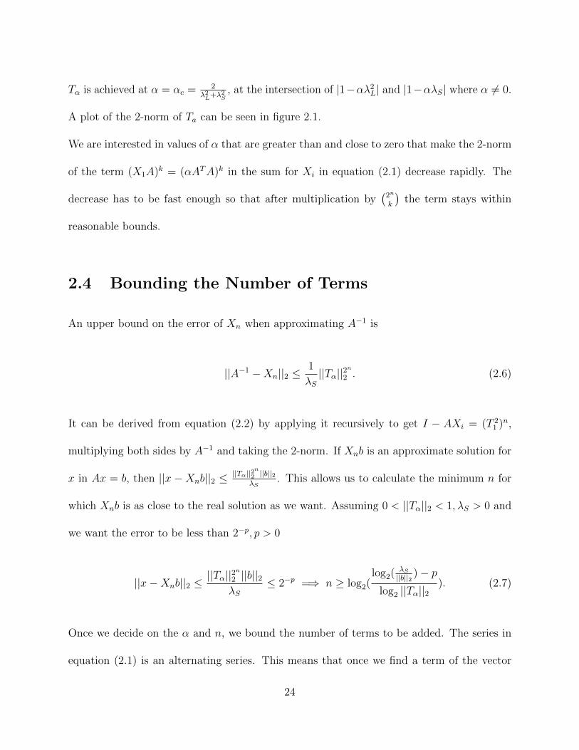
2.4 Bounding the Number of Terms
An upper bound on the error of Xn when approximating A−1 is
||A−1 −Xn||2 ≤1
λS||Tα||2
n
2 . (2.6)
It can be derived from equation (2.2) by applying it recursively to get I − AXi = (T 21 )n,
multiplying both sides by A−1 and taking the 2-norm. If Xnb is an approximate solution for
x in Ax = b, then ||x−Xnb||2 ≤ ||Tα||2n
2 ||b||2λS
. This allows us to calculate the minimum n for
which Xnb is as close to the real solution as we want. Assuming 0 < ||Tα||2 < 1, λS > 0 and
we want the error to be less than 2−p, p > 0
||x−Xnb||2 ≤||Tα||2
n
2 ||b||2λS
≤ 2−p =⇒ n ≥ log2(log2(
λS||b||2 )− p
log2 ||Tα||2). (2.7)
Once we decide on the α and n, we bound the number of terms to be added. The series in
equation (2.1) is an alternating series. This means that once we find a term of the vector
24

sequence that has a ∞-norm, which is equal to the largest absolute value of all the elements
of a vector, that is smaller than 2−p, we can discard the rest of the terms. That happens
when
||(
2n
k
)(−1)k−1(X1A)k−1X1b||∞ ≤
(2n
k
)||X1A||k−1∞ ||X1b||∞ ≤ 2−p,
where ‖X1A‖∞ = max ‖X1Ax‖∞‖x‖∞ , x 6= 0.
Suppose ||X1A||∞ ≤ 2−m and ||X1b||∞ ≤ 2−q. Then we have to find k such that
(2n
k
)||(X1A)||k−1∞ ||X1b||∞ ≤
2nk
k!2−m(k−1)2−q ≤ 2−p
or
−k∑i=1
log2(k) + (n−m)k +m− q ≤ −p.
2.5 Actual results
The method works best when the condition number κ(ATA) (the ratio of the largest and
smallest eigenvalues of ATA) is close to 1, because in that case ||Tα||2 decreases much faster
with increasing α.
For the experiment, a real square matrix A of size 200x200, which was a sum of the identity
matrix and a matrix with elements drawn from a uniformly random distribution, was used.
The test was performed using the GNU Octave software package working with double pre-
cision arithmetic. The smallest eigenvalue of ATA was equal to 0.94405, the largest one was
2.2506 (condition number of 2.38398). For an expression of X6 in terms of X1 only the first
25

Figure 2.2: Plot of the number of terms that have magnitude greater than 2−16 in terms ofn and α.
54 out of 64 terms of equation (2.1) need to be added to get the ∞-norm of the error of the
approximate solution down to less than 2−16. The plot of the number of terms that have
magnitude greater than 2−16 can be seen in Figure 2.2 where α ∈ [0; 0.25] on one horizontal
axis and n ∈ [0; 20] on the other one. It was generated using the code provided in Appendix
A.
Some amount of parallelism in the algorithm could be extracted by doing the summing in-
dependently once you have the terms of the sum ready. Also, even though there is a lot
dependence among the terms themselves, each one can be computed in multiple ways. For
example, the vector term (X1A)8X1b can be found by applying the matrix X1A to X1b
eight times, or multiplying X1A by itself three times to get ((X1A)2)2)2 = (X1A)8 and then
multiplying that by X1b. Whether that is something worth doing needs further investigation.
26

2.6 Problems With This Method
The biggest problem is that the terms in the sequence grow extremely large and this results
in catastrophic cancellation error that causes significant loss of accuracy in the last digits
of the computed solution. For larger values of n and larger condition numbers, zero digits
of accuracy can be computed. One idea to mitigate this cancellation error could be to
orthogonalize the set of basis vectors (X1A)kX1b for k = 0, 1, 2... used in the expansion of
the series. However, all this does is it moves the main problem of computing an alternating
series with coefficients of large magnitude for the solution of Ax = b to computing the
coefficients for the expansion in the new basis. The coefficient for the first vector in this
basis set is now∑2n
k=1
(2n
k
)(−1)k−1αkci where ci = ((X1A)iX1b)
TX1b. It is another alternating
series with coefficients of large magnitude, but its result is now a scalar, not a vector. It is
not clear if it is possible to compute this numerically in a practical way and currently I am
not aware of any way solve the cancellation error problem.
Another disadvantage is that other, more popular Krylov subspace iterative methods, that
will be analysed in more detail in the following chapters, reach the desired accuracy much
quicker compared to the described algorithm and do it in a stable way. By ”stable” we mean
that the solution will not diverge.
27

Chapter 3
Conjugate Gradient Method
The Conjugate Gradient method is an iterative algorithm for finding a solution to a large and
sparse linear system of equations whose corresponding matrix A is real, symmetric (AT = A)
and positive-definite (xTAx > 0 for all non-zero vectors x). In this chapter the algorithm
will be described briefly and a way to reduce the need for synchronization will be introduced.
3.1 The Algorithm
Given a matrix A, a right-hand side vector b and an initial guess at a solution x0 (usu-
ally x0 = b or x0 = 0), the algorithm is trying to minimize the quadratic function f(x) =
12xTAx − xT b. The point that minimizes this function is the actual solution to Ax = b. At
each iteration of the algorithm, a search direction di is chosen so that it is A-orthogonal
to and linearly independent from all the other previous search directions. A-orthogonality
means that dTi Adj = 0 for all j < i.
28

After we find a suitable direction vector dk, a step in that direction is taken xk+1 = xk+αkdk
using an αk that minimizes the quadratic function f(xk+1). Thus, a sequence x0, x1, ..., xk
is generated and xk → x as k → n − 1, where x is the actual solution to Ax = b. The-
oretically, the algorithm reaches the exact solution after n iterations because the search
directions d0, d1, ..., dn−1 cover the whole search space. In practice, however, the floating
point arithmetic used in computers prevents us from finding the exact solution, but we can
get sufficiently close. Pseudocode for the conjugate gradient method is shown in Algorithm
1.
Algorithm 1 Find a solution to Ax = b using the Conjugate Gradient method
Input: matrix A, vector bOutput: solution xnx0 := 0n := row count of Ar0 := b− Ax0d0 := r0k := 0while k < n doαk :=
rTk rkdTkAdk
xk+1 := xk + αkdkrk+1 := rk − αkAdkβk+1 :=
rTk+1rk+1
rTk rk
dk+1 := rk+1 + βk+1dkk := k + 1
end while
Usually the algorithm is stopped after much fewer than n iterations. The magnitude of the
residual rk can be a good indicator of when to halt the program when it drops below some
set threshold. For more information about the stopping criterion as it applies to the finite
element method, see [12].
29

3.1.1 Convergence
After k iterations of the Algorithm 1, an approximate solution xk to x = A−1b is chosen
from the Krylov subspace Kk(A, r0) := span({r0, Ar0, A2r0, ..., Ak−1r0}) such that the error
ek = x− xk is minimized over the A-norm ||ek||A = eTkAek. Expand xk in the form
xk =k−1∑j=0
αjAjr0 (3.1)
given some coefficients α0, α1, ..., αk−1. We can express this as xk = qk−1(A)r0 where qk−1(ζ)
is a polynomial of the form
qk−1(ζ) =k−1∑j=0
αjζj. (3.2)
Since x0 = 0, e0 = x− x0 = x, r0 = b− Ax0 = b and we can express ek as
ek = e0 − xk = e0 − qk−1(A)r0 = pk(A)e0, (3.3)
where pk(ζ) = 1− ζqk−1(ζ) is a polynomial of degree k.
As previously stated, ||ek||A is minimized over all the vectors in the Krylov subspaceKk(A, r0)
and this gives us a way to characterize the polynomial pk(ζ) as a polynomial of order k with
a constant term equal to 1 that minimizes
||ek||A = minpk∈Pk,pk(0)=1
||pk(A)e0||A, (3.4)
30

where Pk is the set of all real polynomials of degree k.
An upper bound on ||ek||A can be found if we expand e0 in the basis of eigenvectors vi of A,
where Avi = λivi:
e0 =n∑j=1
γjvj. (3.5)
Combining the last two equations we can bound the error ek:
‖ek‖A = minpk∈Pk,pk(0)=1 ‖n∑j=1
γjpk(λj)vj‖A
≤ minpk∈Pk,pk(0)=1 ‖maxj |pk(λj)|n∑j=1
γjvj‖A
= minpk∈Pk,pk(0)=1 maxj |pk(λj)|‖e0‖A.
(3.6)
If we can find an interval [a, b] such that λj ∈ [a; b] for all j (optimally a = minj λj, b =
maxj λj), then
‖ek‖A‖e0‖A
≤ minpk∈Pk,pk(0)=1
maxx∈[a;b]
|pk(x)|. (3.7)
Polynomials pk(x) that minimize the upper bound of equation (3.7) are known (see [14]) and
they are a scaled and translated version of Chebyshev polynomials of the first kind:
χk(x) =τk(b+ab−a −
2xb−a
)τk(b+ab−a
) . (3.8)
Standard Chebyshev polynomials τ0, τ1, ... are given by τk(x) = cos(k cos−1 x) and it can be
shown that
τk(x) =1
2
[(t+√t2 − 1)k + (t−
√t2 − 1)k
]. (3.9)
31

If a = minj λj and b = maxj λj, then the condition number of A is κ =maxj λjminj λj
= ba
and using
equation (3.9) we get
τk
(b+ a
b− a
)= τk
(κ+ 1
κ− 1
)=
1
2
[(√κ− 1√κ+ 1
)k+
(√κ+ 1√κ− 1
)k]≥ 1
2
(√κ+ 1√κ− 1
)k. (3.10)
The magnitude of the numerator in equation (3.8) is always less than or equal to one for
x ∈ [a; b] and combining equation (3.7) with (3.8) and (3.10) we can establish the following
upper bound on ‖ek‖A:
‖ek‖A ≤ 2
(√κ− 1√κ+ 1
)k‖e0‖A. (3.11)
This shows that for well-conditioned matrices the conjugate gradient method converges very
quickly. More on the convergence of the conjugate gradient method can be found in [6],
pages 72-75.
3.2 Synchronization Reduction
3.2.1 Theory
The conjugate gradient method is highly synchronous. The computation of dk at iteration
k depends on having already computed βk and rk, βk depends on rk, rk depends on αk−1
and αk−1 depends on dk−1. In this section we will introduce a way to compute the search
direction dk without directly relying on already having rk or xk.
Assume you are doing the k-th iteration so you already have k A-orthogonal search directions
32

d1, d2, ..., dk. Then the next search direction can be computed as follows:
1. Compute q = Adk.
2. A-orthogonalize q and dk to get q′ (q′ = q − dTkAq
dTkAdkdk).
3. A-orthogonalize q′ and dk−1 to get dk+1 (dk+1 = q′ − dTk−1Aq
dTk−1Adk−1dk−1).
dk+1 is automaticallyA-orthogonal to d1, d2, ...dk−2 becauseAdk isA-orthogonal to d1, d2, ...dk−2.
We can prove the A-orthogonality of Adk with dj, j < k − 1 as follows:
Lemma 3.2.1. Assume we are working in infinite precision arithmetic. Then either the set
of vectors Kk = {b, Ab,A2b, ..., Ak−1b} are linearly independent or the solution to Ax = b has
already been found at the k-th iteration of the conjugate gradient method.
Proof. Suppose the set of vectors Kk are not linearly independent for some k and some
vector Aib for i ∈ {0, 1, 2, ..., k − 1} can be expressed as a linear combination of vectors in
{Ajb}j=0,2..i−1 = Ki. This implies that Ai+1b = AAib can also be expressed in terms of
vectors in Ki and span(Ki+1) = span(Ki). The conjugate gradient method chooses xi to
be a linear combination of vectors in Kk such that the residual rk is minimized. The CG
algorithm solves the problem in a finite number of iterations n, rn = 0. As the span of Kk
is the same as of Ki, ri must be zero and the solution has already been found at iteration i
or the vectors in Kk are linearly independent.
Theorem 3.2.2. Assume the solution has not yet been found at the k-th iteration of the
conjugate gradient method. Then Adk is A-orthogonal to d1, d2, ...dk−2 where di is the search
direction used at i’th iteration.
33
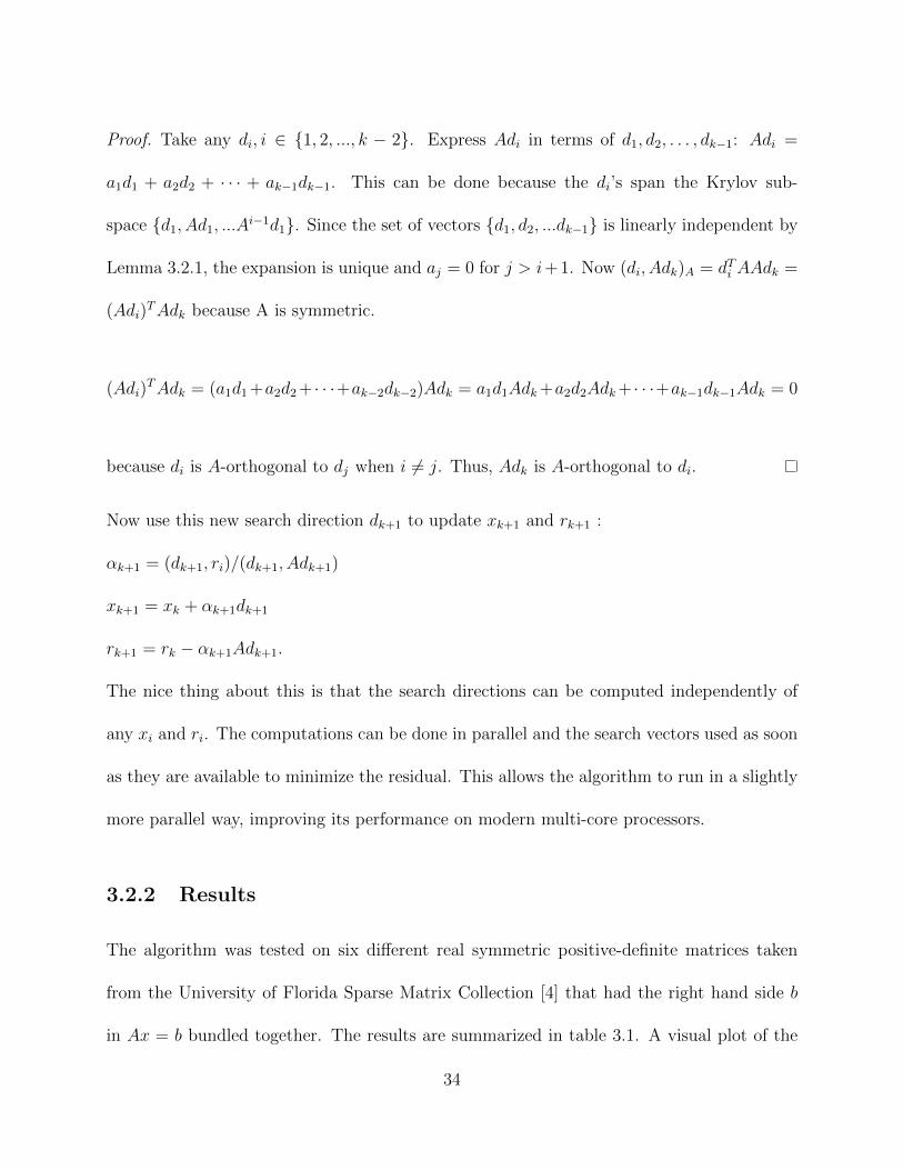
Proof. Take any di, i ∈ {1, 2, ..., k − 2}. Express Adi in terms of d1, d2, . . . , dk−1: Adi =
a1d1 + a2d2 + · · · + ak−1dk−1. This can be done because the di’s span the Krylov sub-
space {d1, Ad1, ...Ai−1d1}. Since the set of vectors {d1, d2, ...dk−1} is linearly independent by
Lemma 3.2.1, the expansion is unique and aj = 0 for j > i+ 1. Now (di, Adk)A = dTi AAdk =
(Adi)TAdk because A is symmetric.
(Adi)TAdk = (a1d1+a2d2+ · · ·+ak−2dk−2)Adk = a1d1Adk+a2d2Adk+ · · ·+ak−1dk−1Adk = 0
because di is A-orthogonal to dj when i 6= j. Thus, Adk is A-orthogonal to di.
Now use this new search direction dk+1 to update xk+1 and rk+1 :
αk+1 = (dk+1, ri)/(dk+1, Adk+1)
xk+1 = xk + αk+1dk+1
rk+1 = rk − αk+1Adk+1.
The nice thing about this is that the search directions can be computed independently of
any xi and ri. The computations can be done in parallel and the search vectors used as soon
as they are available to minimize the residual. This allows the algorithm to run in a slightly
more parallel way, improving its performance on modern multi-core processors.
3.2.2 Results
The algorithm was tested on six different real symmetric positive-definite matrices taken
from the University of Florida Sparse Matrix Collection [4] that had the right hand side b
in Ax = b bundled together. The results are summarized in table 3.1. A visual plot of the
34

Figure 3.1: Residual plot for ”af 3 k101” matrix.
Figure 3.2: Residual plot for ”nasa4704” matrix.
35

Figure 3.3: Residual plot for ”olafu” matrix.
Figure 3.4: Residual plot for ”parabolic fem” matrix.
36

Figure 3.5: Residual plot for ”smt” matrix.
Figure 3.6: Residual plot for ”thermal1” matrix.
37

actual norm of the residual after each iteration can be seen in figures 3.1 to 3.6, where the
horizontal axis is the index of the iteration and the vertical axis is the norm. The decision
about whether the algorithm converges or not was made by visually inspecting the slope of
the graph - if the slope was negative, it was assumed that the estimate of the solution would
eventually converge to the actual solution.
For some of the matrices, the modified algorithm outputs the exact same results as the
original algorithm (matrices ”parabolic fem” and ”thermal1”). However, for others some
numerical instability causes the modified algorithm to explode and produce solution values
outside the normal range (matrices ”af 3 k101”, ”nasa4704”, ”olafu” and ”smt”). The mod-
ified algorithm can be fixed by resetting the estimate of the residual and the search direction
when the solution explodes by setting residual = b − Ax, search direction = residual for
the last known valid solution estimate x, but that makes a significant difference in the output
of the modified algorithm compared to the original algorithm. The source of the numerical
instability is not known right now and needs further investigation.
38

Matrix name Size Non-zeroentries
Original Modified
af 3 k101 503625× 503625 17550675 converges converges, residual = NaNafter 28 iterations, reset ev-ery 20 iterations
nasa4704 4704× 4704 104756 converges converges, residual = NaNafter 25 iterations, reset ev-ery 20 iterations
smt 25710× 25710 3749582 converges converges, residual = NaNafter 28 iterations, reset ev-ery 20 iterations
olafu 16146× 16146 1015156 does notconverge
does not converge,residual = NaN after22 iterations, reset every 10iterations
parabolic fem 525825× 525825 3674625 converges convergesthermal1 82654× 82654 574458 converges converges
Table 3.1: A description of a sample of matrices taken from the University of Florida matrixlibrary and the results of running the modified Conjugate Gradient method on them.
39

Chapter 4
Soft Errors and Conjugate Gradient
Method
As mentioned in the introductory chapter, sometimes computation can be corrupted by soft
errors - one time events that do not halt the algorithm and need extra care to be detected.
In this chapter we will try to modify the standard conjugate gradient method to fix the
erroneous results caused by soft errors once they have been detected.
4.1 Errors as Perturbations to the Matrix
Iterative methods have the property that they might never find the solution in a finite
number of steps but should get closer to the real solution at every step. That is why, when
running an iterative method like the conjugate gradient method, we would want to stop
after some number of iterations and check for soft errors. If no errors have occurred then we
40

may continue. On the other hand, if there is at least one soft error in the computation of
matrix-vector or inner vector products involved in the computation, we would like to be able
to fix it in an efficient way as opposed to restarting the whole algorithm from the beginning
or, if we took care of storing the intermediate results, a point where everything was still
correct.
Suppose we have an equation Ax = b. We would like to construct a sequence of matrices
A1, A2, ..., An such that Ai → A as i → ∞ and for every i, Aixi = bi, where xi is the
computed solution at the i’th iteration of the algorithm and bi is some n × 1 vector that
might differ at each iteration, but is also approaching b. Now, if one soft error occurs during
the computation of the solution and we can detect it using the method described in chapter
1.3, we would like to be able to fix it. If we stopped after j iterations to check for errors, we
have our current erroneous matrix (call it Aej) and erroneous approximation to the solution
(call it xej) that should satisfy Aejxej = bj. We would like to be able to find a rank-1 matrix
δA = uvT such that Aej + δA = Aj. In that case we could find the actual solution at step j
with the help of the Sherman-Morrison formula
(A+ uvT )−1 = A−1 − A−1uvTA−1
1 + vTA−1u. (4.1)
Our goal is to find such a sequence of matrices A1, A2, ...An that would result in an easy-to-
compute rank-1 matrix update δA in case of one soft error.
41
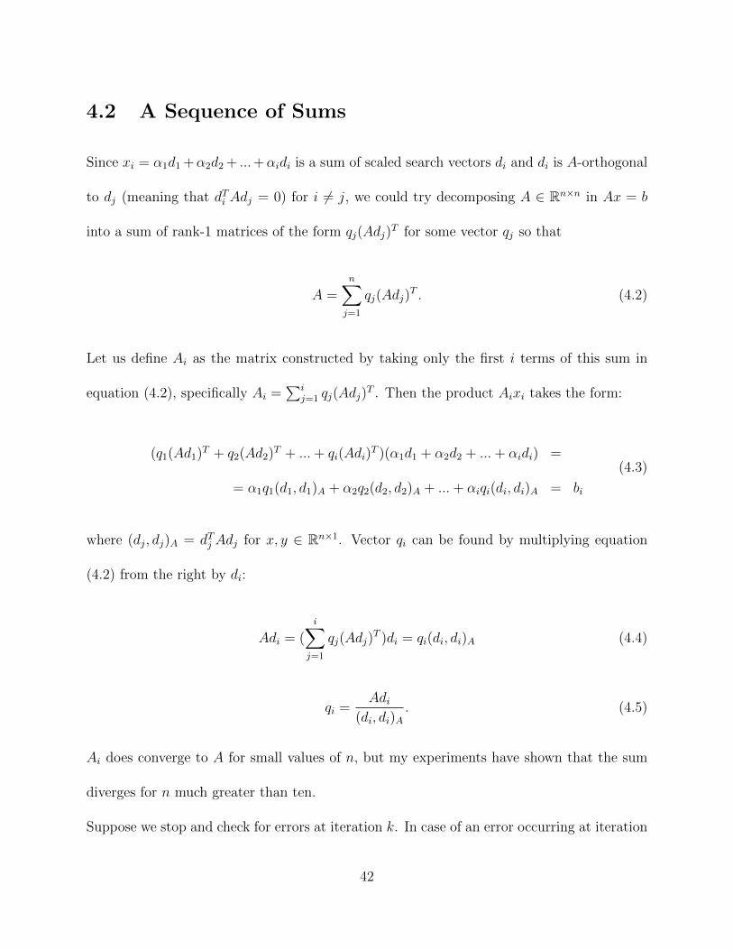
4.2 A Sequence of Sums
Since xi = α1d1 +α2d2 + ...+αidi is a sum of scaled search vectors di and di is A-orthogonal
to dj (meaning that dTi Adj = 0) for i 6= j, we could try decomposing A ∈ Rn×n in Ax = b
into a sum of rank-1 matrices of the form qj(Adj)T for some vector qj so that
A =n∑j=1
qj(Adj)T . (4.2)
Let us define Ai as the matrix constructed by taking only the first i terms of this sum in
equation (4.2), specifically Ai =∑i
j=1 qj(Adj)T . Then the product Aixi takes the form:
(q1(Ad1)T + q2(Ad2)
T + ...+ qi(Adi)T )(α1d1 + α2d2 + ...+ αidi) =
= α1q1(d1, d1)A + α2q2(d2, d2)A + ...+ αiqi(di, di)A = bi
(4.3)
where (dj, dj)A = dTj Adj for x, y ∈ Rn×1. Vector qi can be found by multiplying equation
(4.2) from the right by di:
Adi = (i∑
j=1
qj(Adj)T )di = qi(di, di)A (4.4)
qi =Adi
(di, di)A. (4.5)
Ai does converge to A for small values of n, but my experiments have shown that the sum
diverges for n much greater than ten.
Suppose we stop and check for errors at iteration k. In case of an error occurring at iteration
42

j, k ≥ j, the rank of δA, the matrix that fixes Ak, is 2 × (k − j + 1) as the rank grows by
two at each iteration for which we do not fix the error. The rank is growing because at each
step the approximation Ak to the matrix A is not getting closer to the actual matrix A in
addition to moving away from it. The computation of δA is highly involved and it is of much
higher rank than we want for use with the Sherman-Morrison formula. A different option to
try would be a product of matrices (a factorization) instead of a sum.
4.3 A Sequence of Products
Suppose we could construct a series of matrices A1, A2, ..., Ai such that Ai = ∆Ai ···∆A2∆A1
and
Ai[x1, x2, ..., xi] = [Ax1, Ax2, ..., Axi], 1 ≤ i ≤ n. (4.6)
In this case one could take ∆Ai = I + qidTi , where qi = Adi−Aidi
dTi Aidi.
Unfortunately this decomposition into a product of matrices does not help with the compu-
tation of the rank-1 perturbation matrix in case of an error. The problem is that an error
at step i affects not only the matrix ∆Ai, but also ∆Ai+1,∆Ai+2, ... and so on.
Another approach we can try is computing the rank-1 perturbation ∆A to matrix A as
∆A = uvT where u = αej, v =dTi A
dTi Adi, j is the location of the error in the vector wi = Adi
that is computed in the conjugate gradient method (lines 8 and 10 in Algorithm 1), α is the
magnitude of the error, di is the search vector in the Algorithm 1 at step i and ej is the unit
vector with value one in location j and zero everywhere else. The erroneous vector is then
equal to wei = wi + αej = (A+ ∆A)di.
43

The problem with this approach is that it requires all the vectors di to be A-orthogonal
to each other. However, once an error is introduced at step k, all the subsequent vectors
dk+1, dk+2... are not A-orthogonal to the first i− 2 vectors any more.
An attempt has been made to apply this solution to the GMRES method (see [8] p.548),
but this factorization works only when the search vectors are all A-orthogonal to each other.
The orthogonality property dTi dj = 0 when i 6= j does not seem to be sufficient.
4.4 Key Problems
There are a couple of reasons why the ideas presented do not seem to work in practice. I
will list some of them:
1. Once a soft error occurs, A + ∆A may not be positive definite any more even if A is
and this is a necessary property for the conjugate gradient method to work properly.
This is not a problem for methods that work with indefinite matrices such as GMRES,
but attempts to apply these ideas to those methods have failed as well.
2. If you want to use the Sherman-Morrison formula to fix the error, you still have to
compute A−1u, where u = αej. This is usually no easier than computing the actual
solution to the main problem Ax = b.
3. The condition number of A+∆A becomes very high even for errors of small magnitude.
But the biggest issue, in my opinion, is that the error ei in the solution is, in general, not in
the Krylov subspace of A at iteration i and can not be expressed using the search vectors
44

d1, d2, ..., di that have already been computed.
45

Chapter 5
A Monte Carlo Method
As computers become faster, but at the same time less reliable, entirely different classes
of algorithms might become useful for solving large scale linear algebra problems. In this
chapter we are going to discuss a stochastic algorithm that was inspired by particle filters,
also known as the sequential Monte Carlo method. The algorithm attempts to guess what
the solution might be and then refines the guesses until it gets close enough to the actual
solution.
5.1 Particle Filters
Particle filtering [11],[3] is a Monte Carlo method for performing statistical inference in
models where the state of the system is evolving with time and information about the state
is collected via noisy measurements made at each time step. However, in our case the state
of the system is constant and we will simply perform noisy measurements to estimate the
46
state vector, the true location of the solution to the linear system of equations. We call the
measurements, or guesses, particles and the act of estimating the state vector - filtering.
5.2 The Algorithm
The algorithm will proceed as follows:
1. First we make a set S1 = {xi1} of N random guesses at the solution to the system of
equations.
2. Afterwards, we compute the residual ri1 = b− Axi1 for each guess xi1.
3. The third step is to make a set T = {xi2} of N new guesses by sampling from the set
S1 without replacement. The probability P (xi1) of picking xi1 is proportional to some
function g(x) of the magnitude of the residual, that is P (xi1) =g(||ri1||)N∑j=1
g(||rj1||). We would
like to sample the guesses with smaller residuals more often so we can pick g(x) = e−βx
for some scalar β. In the experiment below, β = 10000.
4. The final step is to apply a small perturbation εi2 to each xi2 ∈ T to form a new set
S2 = {xi2 + εi2 : xi2 ∈ T}. This allows us to search for better solutions in the vicinity of
the current estimate xi2.
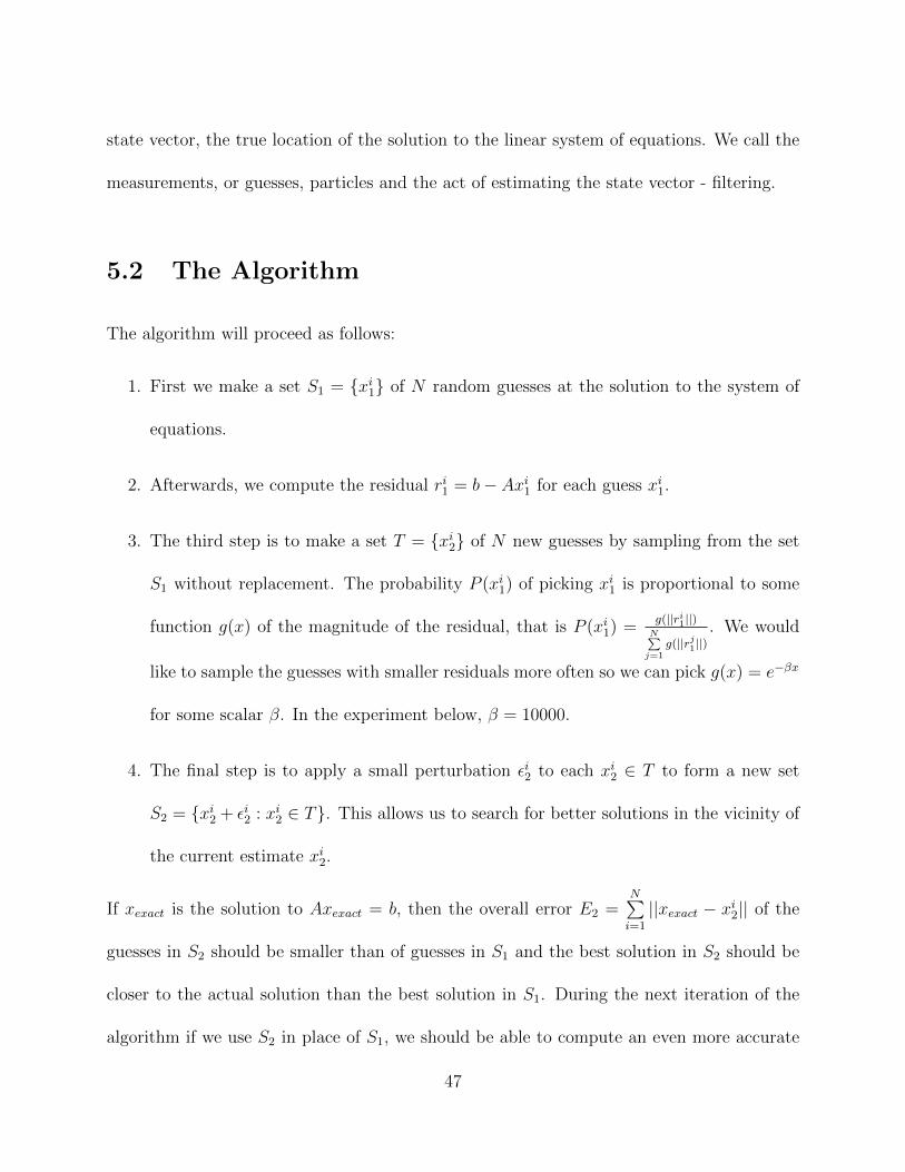
If xexact is the solution to Axexact = b, then the overall error E2 =N∑i=1
||xexact − xi2|| of the
guesses in S2 should be smaller than of guesses in S1 and the best solution in S2 should be
closer to the actual solution than the best solution in S1. During the next iteration of the
algorithm if we use S2 in place of S1, we should be able to compute an even more accurate
47

Figure 5.1: Logarithmic plot of the norm of the smallest residuals at every iteration
solution. We can use the magnitude of the smallest residual to figure out when to stop the
algorithm, just as with the conjugate gradient method discussed in Chapter 3.
5.3 Results
The test was performed using a matrix A = 110B + I ∈ R200×200 which is a sum of a matrix
B ∈ R200×200 with uniformly random elements in the range [0;1) and the 200× 200 identity
matrix I. A logarithmic plot of the smallest norm of the residuals after each iteration can
be seen in Figure 5.1. The magnitude of the smallest residual is steadily decreasing and
this implies that we are computing more and more accurate solutions. Code used for the
experiment can be found in the Appendix C.
48

5.4 Further Work
Careful analysis of the algorithm has not been carried out yet. An investigation into the
convergence bounds similar to the one presented in Chapter 3.1.1 on the conjugate gradient
method would be useful. Also, it is not clear what an optimal function g(x) of the norm of
the residual in step 3 of the algorithm could be.
The algorithm could be potentially useful in cases where a lot of errors occur during execution
time and some form of fault-tolerance is required as it does not matter if some of the solutions
have large errors in them because they will be discarded during the re-sampling step and
replaced with more accurate ones. Also, each sample is independent of every other sample
so a lot of operations could be performed in parallel per sample.
49

Chapter 6
Summary
Even though the modification of the hyperpower method presented in Chapter 2 does not
require any matrix-matrix multiplications to find the solution as opposed to the original
algorithm of finding the inverse of the matrix first, it suffers from cancellation error and is
not usable for large matrices of moderate rank.
The modification of the original Conjugate Gradient method in Chapter 3 reduces some
synchronization and allows the algorithm to run in a more parallel fashion arriving at an
answer quicker on multi-core machines. However, it does fail sometimes as shown during the
experiments.
Recovering from soft errors as formulated in Chapter 4 should allow for faster recovery.
However, I was not able to build a proper procedure for recovery because of some serious
theoretical problems. Also, simply restoring the last known good solution and restarting the
standard algorithm from that point is a simple solution that is hard to improve on.
The Monte Carlo algorithm presented in Chapter 5 does allow easy recovery from soft errors,
50

but is not very efficient considering how many operations it performs for a set level of solution
accuracy. However, it might be practical for processors with very high rates of soft errors.
6.1 Suggestions for Further Work
Fault-tolerance for iterative methods for solving large and sparse linear systems of equations
is still an active topic of research. At the moment the best way to recover from a soft error
after detecting it is restarting from a checkpoint. It would be beneficial to have methods
that are able to recover from one or more soft errors without throwing away all the results
computed after a checkpoint.
Stochastic Monte Carlo methods such as the one presented in Chapter 5 could be fairly
resilient to soft errors because we can treat these errors as just another source of randomness,
but converge slower than the more popular algorithms such as the conjugate gradient method
and are more computationally intensive. Convergence bounds for the method in chapter 5
need to be established and there are a lot of parameters that need investigating and tuning.
51

Bibliography
[1] 754-2008 - IEEE Standard for Floating-Point Arithmetic. Aug. 29, 2008. isbn: 978-0-
7381-5752-8.
[2] M. Altman. “An optimum cubically convergent iterative method of inverting a linear
bounded operator in Hilbert space”. In: Pacific Journal of Mathematics 10 (4 1960),
pp. 1107–1113.
[3] S. Arulampalam et al. “A tutorial on particle filters for online nonlinear/non-Gaussian
Bayesian tracking”. In: IEEE Transactions on Signal Processing 50 (2 2002), pp. 174–
188.
[4] Tim Davis and Yifan Hu. The University of Florida Sparse Matrix Collection.
http://www.cise.ufl.edu/research/sparse/matrices/. 2014.
[5] Peng Du, Piotr Luszczek, and Jack Dongarra. High Performance Linear System Solver
with Resilience to Multiple Soft Errors.
http://www.netlib.org/lapack/lawnspdf/lawn256.pdf. 2011.
52

[6] Howard C. Elman, David J. Silvester, and Andrew J. Wathen. Finite Elements and
Fast Iterative Solvers with Applications in Incompressible Fluid Dynamics. Oxford Uni-
veristy Press, 2005. isbn: 019852868X.
[7] David Goldberg. “What Every Computer Scientist Should Know About Floating-Point
Arithmetic”. In: Computing Surveys (March, 1991).
[8] Gene H. Golub and Charles F. Van Loan. Matrix Computations (3rd Edition). Johns
Hopkins University Press, 1996. isbn: 0801854148.
[9] C. L. Lawson et al. “Basic Linear Algebra Subprograms for Fortran Usage”. In: ACM
Transactions on Mathematical Software (TOMS) 5 (3 1979), pp. 308–323.
[10] Hans Meuer et al. Top500 Supercomputing Sites. http://www.top500.org/.
[11] Emin Orhan. Particle Filtering.
http://www.cns.nyu.edu/~eorhan/notes/particle-filtering.pdf. 2012.
[12] M. Picasso. “A stopping criterion for the conjugate gradient algorithm in the framework
of anisotropic adaptive finite elements”. In: Communications in Numerical Methods in
Engineering 25 (4 2009), pp. 339–355.
[13] David Pool. Linear Algebra: A Modern Introduction (Second Edition). Thomson Brooks/Cole,
2005. isbn: 0534405967.
[14] Theodore J. Rivlin. Chebyshev Polynomials: From Approximation Theory to Algebra
and Number Theory. Wiley-Interscience, 1990. isbn: 0471628964.
53

[15] Jonathan Richard Shewchuk. An Introduction to the Conjugate Gradient Method With-
out the Agonizing Pain.
http://www.cs.cmu.edu/~quake-papers/painless-conjugate-gradient.pdf. 1994.
[16] V. K. Stefanidis and K. G. Margaritis. Algorithm Based Fault Tolerant Matrix Opera-
tions for Parallel and Distributed Systems: Block Checksum Methods.
http://www.academia.edu/1350674. 2003.
54

Appendices
55

Appendix A
Code for the Number of Terms
Code for GNU Octave to compute the number of terms to solve Ax = b:
n = 200; # matrix size n x n
p = 16; # aim for less than 2^-p of absolute error
A = rand(n)*0.005+eye(n); # The Matrix
b = rand(n,1);
m = eigs(A*A’,1,’sm’) # smallest eigenvalue
M = eigs(A*A’,1,’la’) # largest eigenvalue
max_k = 2000; # maximum number of terms that should be added
stepfrac = 400;
steps = 100;
stepsize = 2.0/(M*stepfrac);
normAtA = norm(A’*A,inf);
normAtb = norm(A’*b,inf);
normb = norm(b);
min_it = inf;
min_alpha = inf;
min_terms = inf;
for i=1:steps,# try different alphas
56

realalpha = i*stepsize;
normT(i) = 1.0 - m*realalpha;
iter(i) = realalpha;
for j=1:20,# try different X_j
prec(j) = j;
value(i,j) = -inf;
# can this iteration achieve enough precision? norm(T)^(2^j) > 2^(-p)
if j < log2((log2(m/normb)-p)/log2(normT(i))), continue; end
m_t = ceil(log2(realalpha*normAtA)); # bound X*A
p_t = ceil(log2(realalpha*normAtb)); # bound X*b
printed_already = 0;
sum = 0;
for k=1:2^j,# sum some terms
if k > max_k, break; end
# have we found a small enough term already?
if printed_already == 1, break; end
# tighter sum (bound) than in the article
sum += log2((2^j-k+1)/k);
term_k = sum + m_t*(k-1) + m_t + p_t;
if term_k <= -p,
printed_already = 1;
value(i,j) = k;
if k <= min_terms,# is this the best solution so far globally?
min_terms = k;
min_alpha = realalpha;
min_it = j;
end
end
end
end
end
fprintf("Best results for alpha = %e and %d iterations: %d terms\n",
min_alpha, min_it, min_terms);
surf(prec,iter,value)
57

Appendix B
Modified Conjugate Gradient Method
The first part of the loop is just A-orthogonalization of the next two search directions.
An attempt has been made to make the code as readable as possible at the cost of computing
some quantities a couple of times.
% input: A, b; result: x;
x = b;
k = 1;
r = b - A*x;
p = r;
while k < length(b)+1,
Ap = A*p;
% orthogonalize the next search direciton
q = Ap - ((p’*A*Ap)/(p’*Ap))*p;
if k > 1
q = q - ((prev_p’*A*Ap)/(prev_p’*A*prev_p))*prev_p;
end
% generate a new search direction used in the next iteration
next_p = A*q;
next_p = next_p - ((q’*A*next_p)/(q’*A*q))*q;
next_p = next_p - ((p’*A*next_p)/(p’*A*p))*p;
58

% any r could be used theoretically, but it has to be updated once
% in a while in practise because of finite precision arithmetic
% and search directions losing orthogonality
alpha_1 = (p’*r)/(p’*Ap);
alpha_2 = (q’*r)/(q’*A*q);
x = x + alpha_1*p;
x = x + alpha_2*q;
% could do without updating r if the search directions would not lose
% orthogonality, but that is not the case as the number of iterations
% increases
r = r - alpha_1*Ap;
r = r - alpha_2*A*q;
if norm(r) < 1.0e-13, break, end
prev_p = q;
p = next_p;
k = k + 1;
end
59

Appendix C
Code for the Monte Carlo Method
The algorithm assumes that variables A, b and n have already been initialized.
maxSamples = floor(2*n);
samples = (ones(n,maxSamples)-2.0*rand(n,maxSamples))*norm(b);
k = 1;
while k < 2000,
res = b*ones(1,maxSamples) - A*samples;
for i=(1:maxSamples)
r(i) = norm(res(:,i));
end
sumR = sum(r);
w = r/sumR;
for i=(1:maxSamples),
w(i) = exp(-w(i)*100000.0);
end
choices = randsample(maxSamples,maxSamples,true,w);
for i=(1:maxSamples)
guess = (ones(n,1)-2.0*rand(n,1));
guess = guess/norm(guess);
newSamples(:,i) = samples(:,choices(i)) + guess*r(choices(i))*0.1;
end
60

samples = newSamples;
k = k + 1;
end
61