Iterative finite element approximations of solutions to parabolic equations with nonlocal conditions
22
Nonlinear Analysis 50 (2002) 433 – 454 www.elsevier.com/locate/na Iterative nite element approximations of solutions to parabolic equations with nonlocal conditions Dennis Jackson ∗ Department of Mathematical Sciences, Florida Institute of Technology, 150 West University Boulevard, Melbourne, FL 32901-6975 USA Received 25 February 2000; accepted 4 December 2000 1. Introduction The following nonlocal parabolic equation will be studied: u t + Au = f(x;t ) on Q; u | =0; T0 0 h(x;)u(x;)d + g(T 1 ;:::;T N ; u)= (x); (1.1) where 0 ¡T 0 6 T; is a bounded domain in R n with a smooth boundary ;Q = × (0;T ), and A is a second order elliptic operator, Au = − n i;j=1 @ @x i a ij (x) @u @x j + n i=1 a i (x) @u @x i + a 0 (x)u (1.2) with a ij (x);a i (x) ∈ C ∞ ( ), and h(t;x) ∈ C ∞ ( Q 0 ) where Q 0 = [0;T 0 ] × . ∗ Corresponding author. Tel.: +1-404-674-8091; fax: +1-404-674-7412. E-mail address: [email protected] (D. Jackson). 0362-546X/02/$ - see front matter c 2002 Elsevier Science Ltd. All rights reserved. PII: S0362-546X(01)00741-6
-
Upload
dennis-jackson -
Category
Documents
-
view
213 -
download
1
Transcript of Iterative finite element approximations of solutions to parabolic equations with nonlocal conditions
Nonlinear Analysis 50 (2002) 433– 454www.elsevier.com/locate/na
Iterative �nite element approximations ofsolutions to parabolic equations with
nonlocal conditions
Dennis Jackson∗
Department of Mathematical Sciences, Florida Institute of Technology, 150 West University Boulevard,Melbourne, FL 32901-6975 USA
Received 25 February 2000; accepted 4 December 2000
1. Introduction
The following nonlocal parabolic equation will be studied:
ut + Au=f(x; t) on Q;
u |�=0;
∫ T0
0h(x; �)u(x; �) d�+ g(T1; : : : ; TN ; u)= (x);
(1.1)
where 0¡T06T; � is a bounded domain in Rn with a smooth boundary �;Q=� ×(0; T ), and A is a second order elliptic operator,
Au=−n∑
i; j=1
@@xi
(aij(x)
@u@xj
)+
n∑i=1
ai(x)@u@xi
+ a0(x)u (1.2)
with aij(x); ai(x)∈C∞( 2�), and h(t; x)∈C∞( 2Q0) where Q0 = [0; T0]× �.
∗ Corresponding author. Tel.: +1-404-674-8091; fax: +1-404-674-7412.E-mail address: jackson@zach.�t.edu (D. Jackson).
0362-546X/02/$ - see front matter c© 2002 Elsevier Science Ltd. All rights reserved.PII: S0362 -546X(01)00741 -6
434 D. Jackson / Nonlinear Analysis 50 (2002) 433– 454
The function g: C0((0; T ];L2(�)) → L2(�) will include functions of the form
g(T1; : : : ; TN ; u)=N1∑i=1
hi(x)u(x; Ti) +N∑
i=N1+1
∫ Ti+Ki
Ti
hi(x; �)u(x; �) d�; (1.3)
with 0¡Ti6T for 16 i6N , Ti + Ki6T and 0¡Ti for N1 + 16 i6N; hi(x)∈C∞( 2�), and hi(x; t)∈C∞( 2� × [Ti; Ti + Ki]).An example of a problem of the form (1.1) is the problem of recovering the ini-
tial concentration of a chemical reactant from measurements of the pointwise amountof reaction over a period of time. Let u(x; t) represent the concentration of the re-actant. Assume it reacts with the region proportionally to the concentration at a rateh(x; t)u(x; t). Also, assume the concentration of the chemical satis�es a diDusion equa-tion, the amount of chemical removed when it reacts is at a rate k(x; t)u(x; t), and (x)is the amount of the reaction from time 0 when the chemical is suddenly mixed intothe region to time T0. The problem can be represented by the system
ut + Au=f(x; t)− k(x; t)u;
u |�=0;∫ T0
0h(x; �)u(x; �) d�= (x):
(1.4)
Nonlocal parabolic problems of the form
ut + Au=f(u);
u |�= g(x);
u(x; 0) + g(T1; : : : ; TN ; u)= (x);
(1.5)
where there is a condition connecting the initial value of u to values at later times,have been studied by several authors. Existence and uniqueness of solutions have beenshown by Byszewski [2], Chabrowski [3], Hess [5], Jackson [7], Kerelov [8] andVabishchewich [15]. In [6], the author obtains error estimates for the semidiscrete �niteelement approximation of equations of the form (1.5) where the parabolic equation islinear. Lin [10] uses an iterative �nite diDerence method to approximate solutions tononlocal problems of the form (1.5).In this paper, it will be shown that system (1.1) has a unique solution under suit-
able conditions on the data. We then approximate the system by a nonlocal system ofordinary diDerential equations and obtain error estimates for the semidiscrete approxi-mation of the solution. Finally, we use a fully discrete iterative procedure to approx-imate u(x; 0). The solution to system (1.1) can then be approximated using standardnumerical methods.
2. Existence and uniqueness of solutions
In this section, the Banach �xed point theorem is used to show the existence anduniqueness of solutions to Eqs. (1.1).
D. Jackson / Nonlinear Analysis 50 (2002) 433– 454 435
Let a(u; v) be de�ned by
a(u; v)=n∑
i; j=1
∫�
aij(x)@u@xi
@v@xj
dx +n∑
i=1
∫�
ai(x)@u@xi
v dx +∫�a0(x)uv dx: (2.1)
Assume for u∈H 10 (�),
a(u; u)¿ �‖u‖21; (2.2)
where Hs(�) and Hs0(�) are the usual Sobolev spaces with norms ‖ ‖s and ‖ ‖= ‖ ‖0,
see [1] or [11].If inequality (2.2) is not satis�ed, but
a(u; u) + 0‖u‖2¿ �‖u‖21;replace u by e 0tw in Eqs. (1.1) and A by 2A=A+ 0I .
Conditions (1.2) and (2.2) imply A with domain, D(A)=H 2(�)∩H 10 (�), generates
an analytic semigroup S(t)= e−At . The fractional powers of A are de�ned. If A satis-�es the inequality (2.2), f∈D(A%); %¿ 0 and 0¡%¡�, one can �nd a constant M'
depending continuously on � for each ' such that
‖A%S(t)f‖6Ma'e−at
t'‖f‖D(A%′ ); (2.3)
where '= % − %′; '¿ 0. See Pazy [12]. In the case A is positive self-adjoint withsmallest eigenvalue �, we can take Ma
' =(�'=(� − a))'e−'.Let the spaces W*;% be de�ned by
W*;a = {f∈C0((0; T ];L2(�)) | sup0¡t6T
t1+*‖f(t)‖¡∞} (2.4)
with Wa =W0; a and norms
‖f‖W*; a = sup0¡t6T
t1+*eat‖f(t)‖: (2.5)
Let a be a constant such that inequality (2.3) is satis�ed. We will assume g :Wa →L2(�) such that for u; v∈Wa,
‖g(T1; : : : ; TN ; u)− g(T1; : : : ; TN ; v)6 k*1 ‖u− v‖W*; a ; *=0: (2.6)
If g is of the form (1.3), then inequality (2.6) is satis�ed for *¿ 0 with constantk*1 given by
k*1 =
N1∑i=1
mi
T 1+*i
e−aTi +N∑
i=N1+1
∫ Ti+Ki
Ti
Hi(�)�1+* ea� d�; (2.7)
where mi =supx∈�|hi(x)| and Hi(t)= supx∈�|hi(x; t)|.Assume
h(x; t)= 1 + k(x; t) (2.8)
436 D. Jackson / Nonlinear Analysis 50 (2002) 433– 454
with k(x; 0)=0, and
‖e−AT0‖¡ 1 (i:e:; Ma0 e
−aT0 ¡ 1): (2.9)
If A is self-adjoint and condition (2.2) is satis�ed, inequality (2.9) holds for allT0; T0 ¿ 0. If condition (2.9) is not satis�ed, replace u by e 0tv for 0¿ 0 large enough.This, however, can increase the size of k*
1 for the new nonlocal function g.If u∈C0([0; T ];L2(�)) satis�es system (1.1) with f∈L1(0; T ;L2(�)), then
u(x; t)= S(t)u(0) +∫ t
0S(t − �)f(x; �) d�: (2.10)
The third condition in the system can be written as∫ T0
0S(�)u(0) d�+
∫ T0
0
∫ �
0h(x; �)S(�− �′)f(x; �′) d�′ d�
+∫ T0
0k(x; �)S(�)u(0) d�+ g(T1; : : : ; TN ; u)= (x): (2.11)
Inequalities (2.2) and (2.9) imply A−1 and (I − e−AT0 )−1 exist. Let
F(u)≡ (I − e−AT0 )−1[ (x)− g(T1; : : : ; TN ; u)−
∫ T0
0k(x; �)u(�) d�
]
−∫ T0
0
∫ �
0(I − e−AT0 )−1(e−A(�−�′)f(x; �′)) d�′ d�: (2.12)
Since A−1 exists,∫ T0
0S(�)u(0) d�=A−1(I − e−AT0 )u(0):
Thus, if the right-hand side of identity (2.12) is a member of D(A), Eqs. (2.10) and(2.11) are equivalent to
u(t)= S(t)AF(u) +∫ t
0S(t − �)f(x; �) d�: (2.13)
Recall, for 0¡.¡ 1; C.([0; T ];L2(�))= {f∈C0([0; T ];L2(�))| ‖f(t) − f(s)‖6L | t − s|.} for some L¿ 0, where L is independent of s and t.We will use the following lemmas:
Lemma 2.1. Let f∈C0([0; T ];D(A%)); %¿ 0, such that A%f∈C.([0; T ];L2(�)) forsome .; 0¡.¡ 1. Let h∈C∞( 2Q) and assume for each t; 06 t6T0; h(x; t)v∈D(A%+1) if v∈D(A%+1). Then∫ T0
0
∫ �
0h(x; �)e−A(�−�′)f(x; �′) d�′ d�∈D(A%+1):
D. Jackson / Nonlinear Analysis 50 (2002) 433– 454 437
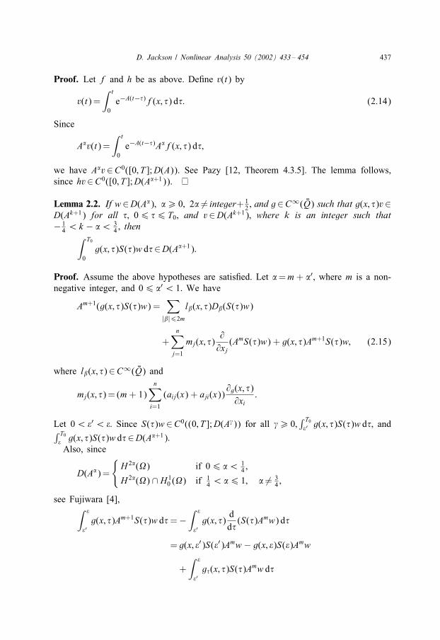
Proof. Let f and h be as above. De�ne v(t) by
v(t)=∫ t
0e−A(t−�)f(x; �) d�: (2.14)
Since
A%v(t)=∫ t
0e−A(t−�)A%f(x; �) d�;
we have A%v∈C0([0; T ];D(A)). See Pazy [12, Theorem 4:3:5]. The lemma follows,since hv∈C0([0; T ];D(A%+1)).
Lemma 2.2. If w∈D(A%); %¿ 0; 2% �= integer+12 ; and g∈C∞( 2Q) such that g(x; �)v∈
D(Ak+1) for all �; 06 �6T0; and v∈D(Ak+1); where k is an integer such that− 1
4 ¡k − %¡ 34 ; then∫ T0
0g(x; �)S(�)w d�∈D(A%+1):
Proof. Assume the above hypotheses are satis�ed. Let %=m+ %′; where m is a non-negative integer, and 06 %′ ¡ 1: We have
Am+1(g(x; �)S(�)w) =∑
|*|62m
l*(x; �)D*(S(�)w)
+n∑
j=1
mj(x; �)@@xj
(AmS(�)w) + g(x; �)Am+1S(�)w; (2.15)
where l*(x; �)∈C∞( 2Q) and
mj(x; �)= (m+ 1)n∑
i=1
(aij(x) + aji(x))@g(x; �)@xi
:
Let 0¡2′ ¡2: Since S(�)w∈C0((0; T ];D(A.)) for all .¿ 0;∫ T0
2′ g(x; �)S(�)w d�; and∫ T0
2 g(x; �)S(�)w d�∈D(A%+1):Also, since
D(A%)=
{H 2%(�) if 06 %¡ 1
4 ;
H 2%(�) ∩ H 10 (�) if 1
4 ¡%6 1; % �= 34 ;
see Fujiwara [4],∫ 2
2′g(x; �)Am+1S(�)w d�=−
∫ 2
2′g(x; �)
dd�
(S(�)Amw) d�
= g(x; 2′)S(2′)Amw − g(x; 2)S(2)Amw
+∫ 2
2′g�(x; �)S(�)Amw d�
438 D. Jackson / Nonlinear Analysis 50 (2002) 433– 454
and S(�)w∈C0([0; T ];H 2%(�));∥∥∥∥A%+1∫ 2
2′g(x; �)S(�)w d�
∥∥∥∥6C∥∥∥∥Am+1
∫ 2
2′g(x; �)S(�)w d�
∥∥∥∥2%′
6∑
|*|62m
∫ 2
2′‖l*(x; .)D*(S(�)w)‖2%′ d�
+n∑
j=1
C∫ 2
2′‖AmS(�)w‖1+2%′ d�
+ ‖ g(x; 2′)S(2′)w − g(x; 2)S(2)w‖2%′
+∫ 2
2′‖g�(x; �)S(�)Amw‖2%′ d�
6C(2− 2′) +n∑
j=1
C∫ 2
2′‖A1=2S(�)Am+%′w‖ d�
6C(2− 2′) +n∑
j=1
C∫ 2
2′
1�1=2
‖S(�)w‖D(A%) d�
6C(2− 2′):
The lemma follows since A%+1 is a closed operator.
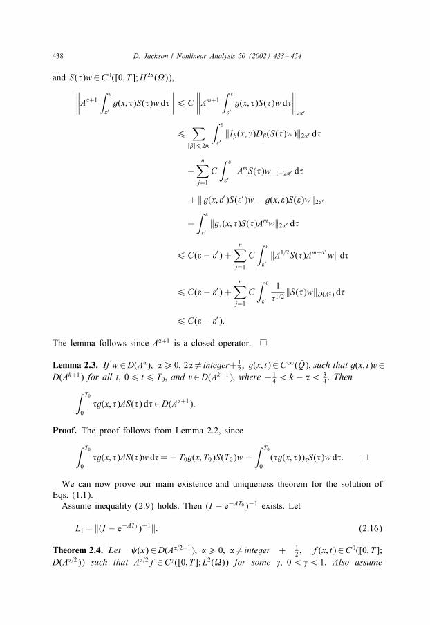
Lemma 2.3. If w∈D(A%); %¿ 0; 2% �= integer+12 ; g(x; t)∈C∞( 2Q); such that g(x; t)v∈
D(Ak+1) for all t; 06 t6T0; and v∈D(Ak+1); where − 14 ¡k − %¡ 3
4 : Then∫ T0
0�g(x; �)AS(�) d�∈D(A%+1):
Proof. The proof follows from Lemma 2.2, since
∫ T0
0�g(x; �)AS(�)w d�=− T0g(x; T0)S(T0)w −
∫ T0
0(�g(x; �))�S(�)w d�:
We can now prove our main existence and uniqueness theorem for the solution ofEqs. (1.1).Assume inequality (2.9) holds. Then (I − e−AT0 )−1 exists. Let
L1 = ‖(I − e−AT0 )−1‖: (2.16)
Theorem 2.4. Let (x)∈D(A%=2+1); %¿ 0; % �= integer + 12 , f(x; t)∈C0([0; T ];
D(A%=2)) such that A%=2f∈C.([0; T ];L2(�)) for some .; 0¡.¡ 1: Also assume
D. Jackson / Nonlinear Analysis 50 (2002) 433– 454 439
conditions (1:2); (2:2); (2:3); (2:6) and (2:9): Assume g(T1; : : : ; TN ; u)∈D(A%=2+1),u∈C0([0; T ]; D(A%=2+1)); and let k(t)=maxx∈�|k(x; t)|: Then if
M%1 L1k01 +Ma
1 L1
∫ T0
0�−1k(�)e−a� d�¡ 1; (2.17)
Eqs. (1.1) have a unique solution u; such that
u∈C0([0; T ];D(A%=2)) ∩ C1((0; T ];D(A%=2)) ∩ C0((0; T ];D(A%=2+1)): (2.18)
Proof. Assume the above hypotheses are satis�ed. For u∈W0; a; de�ne 3(u) by
3(u)=AS(t)F(u) +∫ t
0S(t − �)f(x; �) d�; (2.19)
where F(u) is de�ned by identity (2.12). Since F(u)∈L2(�); and ‖AS(t)F(u)‖6 (Ma
1 =t)‖F(u)‖; it follows that 3(u)∈W0; a:Let u; v∈W0; a: Then
‖teat(3(u)(t)− 3(v)(t))‖6Ma
1 L1‖g(T1; : : : ; TN ; u)− g(T1; : : : ; TN ; v‖
+Ma1 L1
∥∥∥∥∫ T0
0k(x; �)(u(�)− v(�)) d�
∥∥∥∥6Ma
1 L1k01‖u− v‖W0; a +Ma1 L1
∫ T0
0�−1 k(x; �)
ea�‖�ea�(u(�)− v(�))‖ d�
6Ma1 L1k01‖u− v‖W0; a +Ma
1 L1
∫ T0
0�−1k(�)e−a� d�‖u− v‖W0; a
6d‖u− v‖W0; a ;
where 0¡d¡ 1:Thus by the Banach �xed point theorem, there is a unique u∈W 1
0; a such thatu=3(u):Then by Eq. (2.19)
∫ T0
0k(x; �)u(�) d�=
∫ T0
0k(x; �)AS(�)F(u) d�+
∫ T0
0k(x; �)v(�) d�;
where v(t) is de�ned by Eq. (2.14). From the above and Lemmas 2.1 and 2.3, it fol-lows that if F(u)∈D(Ai); 06 i6 %=2+ 1 then
∫ T0
0 k(x; �)u(�) d�∈D(Ai+1): ThereforeF(u)∈D(A%=2+1); which implies conclusions (2.18).
If inequality (2.17) is not satis�ed, system (1.1) may not have a unique solution.
440 D. Jackson / Nonlinear Analysis 50 (2002) 433– 454
Example. Consider the system
ut − uxx =0; if 0¡x¡ 1;
u(0; t)= 0; u(1; t)= 0;∫ 1
0u(x; �) d�− bu(x; 2)= (x) (2.20)
for a= 62− 12 ; Ma
1 = 262e−1: Also L1 = (1−e−62)−1 and k01 = (b=2)e−262+1: Thus, Eqs.
(2.20) have a unique solution if (x)∈H 2(0; 1)∩H 10 (0; 1) and b62e−262
=(1−e−62)¡ 1:
But if b=(1 − e−62)=62e−262
; then u(x; t)=Ae−62t sin 6x satis�es Eqs. (2.20) with (x) ≡ 0 for all values of A and the system has no solution if (x)= sin 6x:
3. The semidiscrete approximation
In this section, we approximate system (1.1) by a nonlocal system of diDeren-tial equations. Under suitable conditions we show the system we use to approximatethe nonlocal problem (1.1) also has a unique solution. Finally, we obtain error esti-mates for the semidiscrete approximations, using semigroup methods similar to those ofLasiecka [9].Let {Vh} be a family of �nite dimensional vector spaces such that Vh ⊆ H 1(�) and
inf8∈Vh
{‖f − 8‖+ h‖f − 8‖1}6Chs‖f‖s (3.1)
for f∈Hs(�) ∩ H 10 (�); 16 s6 r; where C is independent of h.
Assume there are linear operators Ah from Vh into itself for h small enough suchthat for fh; gh ∈Vh and 2¿ 0
(Ahfh; fh)¿ �′‖fh‖21 (3.2)
with
�6 �′ + 2; (3.3)
(Ahfh; gh)6C‖fh‖1‖gh‖1 (3.4)
and
‖(PhA−1 − A−1h Ph)f‖6Ch%+2‖A%=2f‖; 06 %6 r − 2; (3.5)
where Ph is the L2 projection of L2(�) onto Vh and C is independent of h in eachcase.The above conditions are satis�ed with �′ in inequality (3.2) equal to � in inequality
(2.2) for the standard Galerkin method. They are also satis�ed if Nitsche’s method is
D. Jackson / Nonlinear Analysis 50 (2002) 433– 454 441
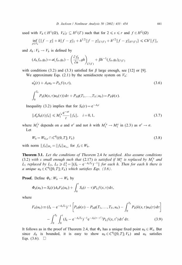
used with Vh ∈H 1(�); Vh|� ⊆ H 1(�) such that for 26 s6 r and f∈H 2(�)
inf8∈Vh
{‖f − 8‖+ h‖f − 8‖1 + h1=2‖f − 8‖L1(�) + hs=2‖f − 8‖H 1(�)}6Chs‖f‖s
and Ah :Vh → Vh is de�ned by
(Ahfh; gh)= a(fh; gh)−(@fh
@n; gh)L2(�)
+ *h−1(fh; gh)L2(�)
with conditions (3.2) and (3.3) satis�ed for * large enough, see [12] or [9].We approximate Eqs. (2.1) by the semidiscrete system on Vh:
u′h(t) + Ahuh =Phf(x; t); (3.6)
∫ T0
0Ph(h(x; �)uh(�)) d�+ Phg(T1; : : : ; TN ; uh)=Ph (x):
Inequality (3.2) implies that for Sh(t)= e−Aht
‖AihSh(t)fh‖6M
′a1e−at
t‖fh‖; i=0; 1; (3.7)
where M′a1 depends on a and �′ and not h with M
′a1 → Ma
1 in (2.3) as �′ → �:Let
Wh =W0; a ∩ C0((0; T ];Vh) (3.8)
with norm ‖fh‖Wh = ‖fh‖W0; a for fh ∈Wh:
Theorem 3.1. Let the conditions of Theorem 2:4 be satis7ed. Also assume conditions(3:2) with 2 small enough such that (2:17) is satis7ed if Ma
1 is replaced by M′a1 and
L1 replaced by L2; L2¿Lh1 = ‖(Ih − e−AhT0 )−1‖ for each h. Then for each h there is
a unique uh ∈C0([0; T ];Vh) which satis7es Eqs. (3.6).
Proof. De�ne 3h :Wh → Wh by
3h(uh)= Sh(t)AhFh(uh) +∫ t
0Sh(t − �)Phf(x; �) d�;
where
Fh(uh)≡ (Ih − e−AhT0 )−1[Ph (x)− Phg(T1; : : : ; TN ; uh)−
∫ T0
0Ph(k(x; �)uh(�) d�
]
−∫ T0
0
∫ �
0(Ih − e−AhT0 )−1e−Ah(�−�′)Phf(x; �′) d�′ d�: (3.9)
It follows as in the proof of Theorem 2.4, that 3h has a unique �xed point uh ∈Wh: Butsince Ah is bounded, it is easy to show uh ∈C0([0; T ];Vh) and uh satis�esEqs. (3.6).
442 D. Jackson / Nonlinear Analysis 50 (2002) 433– 454
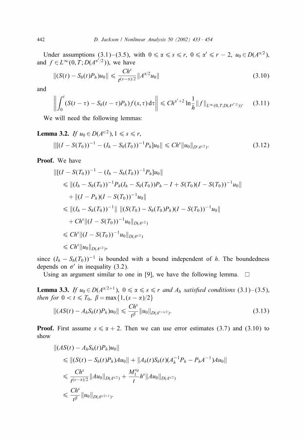
Under assumptions (3.1)–(3.5), with 06 %6 s6 r; 06 %′6 r − 2; u0 ∈D(A%=2);and f∈L∞(0; T ;D(A%′=2)); we have
‖(S(t)− Sh(t)Ph)u0‖6 Chs
t(s−%)=2 ‖A%=2u0‖ (3.10)
and ∥∥∥∥∫ t
0(S(t − �)− Sh(t − �)Ph)f(x; �) d�
∥∥∥∥6Ch%′+2 ln1h‖f‖L∞(0;T ;D(A%′ =2)): (3.11)
We will need the following lemmas:
Lemma 3.2. If u0 ∈D(As=2); 16 s6 r;
‖[(I − S(T0))−1 − (Ih − Sh(T0))−1Ph]u0‖6Chs‖u0‖D(As=2): (3.12)
Proof. We have
‖[(I − S(T0))−1 − (Ih − Sh(T0))−1Ph]u0‖6 ‖(Ih − Sh(T0))−1Ph(Ih − Sh(T0))Ph − I + S(T0)(I − S(T0))−1u0‖+ ‖(I − Ph)(I − S(T0))−1u0‖
6 ‖(Ih − Sh(T0))−1‖ ‖(S(T0)− Sh(T0)Ph)(I − S(T0))−1u0‖+Chs‖(I − S(T0))−1u0‖D(As=2)
6Chs‖(I − S(T0))−1u0‖D(As=2)
6Chs‖u0‖D(As=2);
since (Ih − Sh(T0))−1 is bounded with a bound independent of h. The boundednessdepends on �′ in inequality (3.2).Using an argument similar to one in [9], we have the following lemma.
Lemma 3.3. If u0 ∈D(A%=2+1); 06 %6 s6 r and Ah satis7ed conditions (3:1)–(3:5);then for 0¡t6T0; *=max{1; (s− %)=2}
‖(AS(t)− AhSh(t)Ph)u0‖6 Chs
t*‖u0‖D(A1+%=2): (3.13)
Proof. First assume s6 % + 2. Then we can use error estimates (3.7) and (3.10) toshow
‖(AS(t)− AhSh(t)Ph)u0‖6 ‖(S(t)− Sh(t)Ph)Au0‖+ ‖Ah(t)Sh(t)(A−1
h Ph − PhA−1)Au0‖
6Chs
t(s−%)=2 ‖Au0‖D(A%=2) +M ′a
1
ths‖Au0‖D(A%=2)
6Chs
t*‖u0‖D(A%=2+1):
D. Jackson / Nonlinear Analysis 50 (2002) 433– 454 443
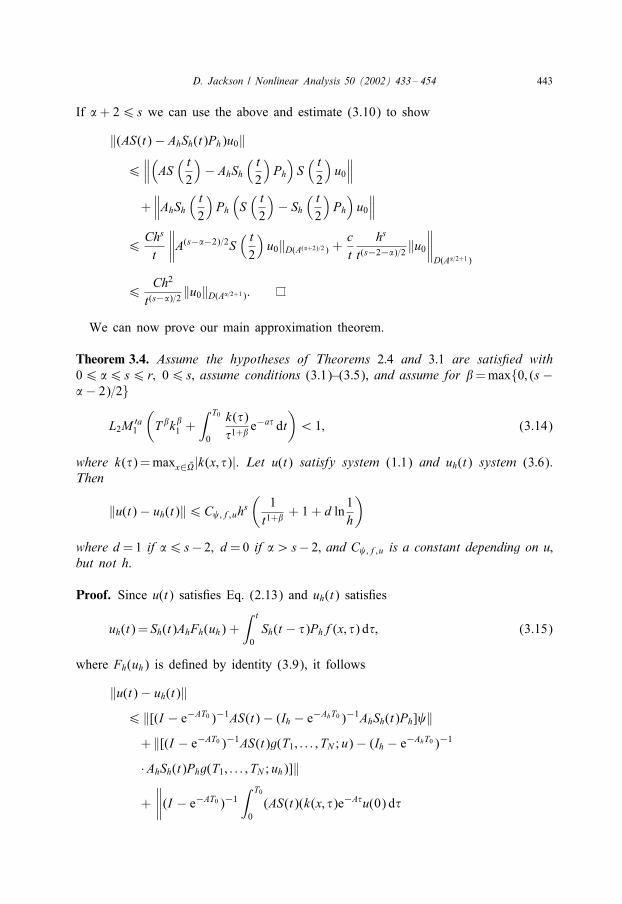
If %+ 26 s we can use the above and estimate (3.10) to show
‖(AS(t)− AhSh(t)Ph)u0‖
6∥∥∥(AS ( t
2
)− AhSh
( t2
)Ph
)S( t2
)u0∥∥∥
+∥∥∥AhSh
( t2
)Ph
(S( t2
)− Sh
( t2
)Ph
)u0∥∥∥
6Chs
t
∥∥∥∥A(s−%−2)=2S( t2
)u0‖D(A(%+2)=2) +
ct
hs
t(s−2−%)=2 ‖u0∥∥∥∥D(A%=2+1)
6Ch2
t(s−%)=2 ‖u0‖D(A%=2+1):
We can now prove our main approximation theorem.
Theorem 3.4. Assume the hypotheses of Theorems 2:4 and 3:1 are satis7ed with06 %6 s6 r; 06 s; assume conditions (3:1)–(3:5), and assume for *=max{0; (s−%− 2)=2}
L2M ′a1
(T*k*
1 +∫ T0
0
k(�)�1+* e
−a� dt)
¡ 1; (3.14)
where k(�)=maxx∈ 2�|k(x; �)|. Let u(t) satisfy system (1:1) and uh(t) system (3:6).Then
‖u(t)− uh(t)‖6C ;f;uhs(
1t1+* + 1 + d ln
1h
)
where d=1 if %6 s− 2; d=0 if %¿s− 2; and C ;f;u is a constant depending on u;but not h.
Proof. Since u(t) satis�es Eq. (2.13) and uh(t) satis�es
uh(t)= Sh(t)AhFh(uh) +∫ t
0Sh(t − �)Phf(x; �) d�; (3.15)
where Fh(uh) is de�ned by identity (3.9), it follows
‖u(t)− uh(t)‖6 ‖[(I − e−AT0 )−1AS(t)− (Ih − e−AhT0 )−1AhSh(t)Ph] ‖+ ‖[(I − e−AT0 )−1AS(t)g(T1; : : : ; TN ; u)− (Ih − e−AhT0 )−1
·AhSh(t)Phg(T1; : : : ; TN ; uh)]‖
+∥∥∥∥(I − e−AT0 )−1
∫ T0
0(AS(t)(k(x; �)e−A�u(0) d�
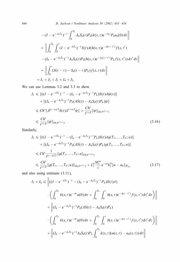
444 D. Jackson / Nonlinear Analysis 50 (2002) 433– 454
− (I − e−AhT0 )−1∫ T0
0AhSh(t)Ph(k(x; �)e−Ah�Phuh(0) d�
∥∥∥∥+∥∥∥∥∫ T0
0
∫ �
0(I − e−AT0 )−1S(t)A(h(x; �)e−A(�−�′)f(x; �′)
− (Ih − e−AhT0 )−1AhSh(t)Ph(h(x; �)e−Ah(�−�′)Phf(x; �′)) d�′ d�∥∥∥
+∥∥∥∥∫ t
0(S(t − �)− Sh(t − �)Ph)f(x; �) d�
∥∥∥∥= I1 + I2 + I3 + I4 + I5:
We can use Lemmas 3.2 and 3.3 to show
I16 ‖((I − e−AT0 )−1 − (Ih − e−AhT0 )−1Ph)S(t)A (x)‖+ ‖(Ih − e−AhT0 )−1Ph(AS(t)− AhSh(t)Ph) ‖
6Chs‖A(s−%)=2S(t)A1+%=2 ‖+ Chs
t1+* ‖ ‖D(A%=2+1)
6Chs
t1+* ‖ ‖D(A%=2+1): (3.16)
Similarly,
I26 ‖((I − e−AT0 )−1 − (Ih − e−AhT0 )−1Ph)S(t)Ag(T1; : : : ; TN ; u)‖+ ‖(Ih − e−AhT0 )−1Ph(AS(t)− AhSh(t)Ph)g(T1; : : : ; TN ; u)‖
6Chs 1t(s−%)=2 ‖g(T1; : : : ; TN ; u‖D(A1+%=2)
6Chs
t1+* ‖g(T1; : : : ; TN ; u)‖D(A%=2+1) + Lh1M ′a
1
te−atk*
1 ‖u− uh‖W*; a (3.17)
and also using estimate (3.11),
I3 + I46∥∥∥∥((I − e−AT0 )−1 − (Ih − e−AhT0 )−1Ph)S(t)A)
·(∫ T0
0k(x; �)e−A�u(0) d�+
∫ T0
0
∫ �
0h(x; �)e−A(�−�′)f(x; �′) d�′ d�
)∥∥∥∥+∥∥∥∥(Ih − e−AhT0 )−1Ph(AS(t)− AhSh(t)Ph)
·(∫ T0
0k(x; �)e−A�u(0) d�+
∫ T0
0
∫ �
0h(x; �)e−A(�−�′)f(x; �′) d�′ d�
)∥∥∥∥+∥∥∥∥(Ih − e−AhT0 )−1AhSh(t)Ph
∫ T0
0k(x; �)(u(x; �)− uh(x; �)) d�
∥∥∥∥
D. Jackson / Nonlinear Analysis 50 (2002) 433– 454 445
+∥∥∥∥(Ih − e−AhT0 )−1AhSh(t)Ph
∫ T0
0
∫ �
0(e−A(�−�′)
− e−Ah(�−�′)Ph)f(x; �′) d�′ d�∥∥∥
6Chs(
1t1+*
)∥∥∥∥∫ T0
0k(x; �) e−A�u(0) d�
+∫ T0
0
∫ �
0h(x; �)e−A(�−�′)f(x; �′) d�′ d�
∥∥∥∥D(A%=2+1)
+L2M ′a
1 e−at
t
∫ T0
0
k(�)�1+* e−a�‖u− uh‖W*; a d�
+Cth%+2 ln 1
h‖f‖L∞(0;T ;D(A%=2)): (3.18)
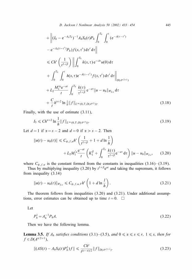
Finally, with the use of estimate (3.11),
I56Ch%+2 ln1h‖f‖L∞(0;T ;D(A%=2)): (3.19)
Let d=1 if %= s− 2 and d=0 if %¿s− 2. Then
‖u(t)− uh(t)‖6C ;f;uhs(
1t1+* + 1 + d ln
1h
)
+L2M′a1e−at
t
(K*1 +
∫ T0
0
k(�)�1+* e
−a� d�)‖u− uh‖W*; a ; (3.20)
where C ;f;u is the constant formed from the constants in inequalities (3.16)–(3.19).Thus by multiplying inequality (3.20) by t1+*eat and taking the supremum, it follows
from inequality (3.14)
‖u(t)− uh(t)‖W*; a 6C ;f;u;T hs(1 + d ln
lh
): (3.21)
The theorem follows from inequalities (3.20) and (3.21). Under additional assump-tions, error estimates can be obtained up to time t=0.
Let
P1h =A−1
h PhA: (3.22)
Then we have the following lemma.
Lemma 3.5. If Ah satis7es conditions (3.1)–(3.5); and 06 %6 s6 r; 16 s; then forf∈D(A%=2+1);
‖(AS(t)− AhSh(t)P1h)f‖6
Chs
t(s−%)=2 ‖f‖D(A%=2+1): (3.23)
446 D. Jackson / Nonlinear Analysis 50 (2002) 433– 454
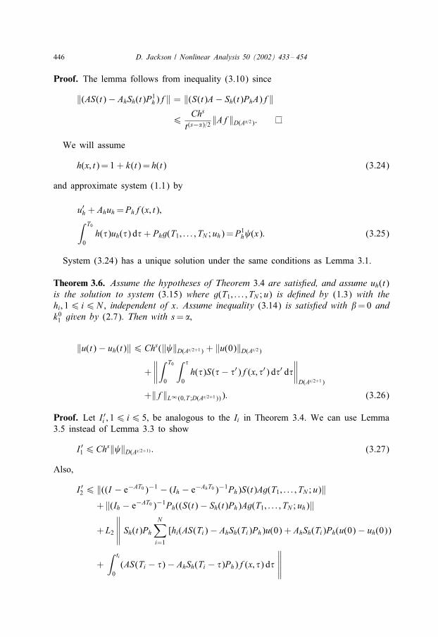
Proof. The lemma follows from inequality (3.10) since
‖(AS(t)− AhSh(t)P1h)f‖ = ‖(S(t)A− Sh(t)PhA)f‖
6Chs
t(s−%)=2 ‖Af‖D(A%=2):
We will assume
h(x; t)= 1 + k(t)= h(t) (3.24)
and approximate system (1.1) by
u′h + Ahuh =Phf(x; t);∫ T0
0h(�)uh(�) d�+ Phg(T1; : : : ; TN ; uh)=P1
h (x): (3.25)
System (3.24) has a unique solution under the same conditions as Lemma 3:1.
Theorem 3.6. Assume the hypotheses of Theorem 3:4 are satis7ed, and assume uh(t)is the solution to system (3.15) where g(T1; : : : ; TN ; u) is de7ned by (1.3) with thehi; 16 i6N , independent of x. Assume inequality (3:14) is satis7ed with *=0 andk01 given by (2.7). Then with s= %;
‖u(t)− uh(t)‖6Chs(‖ ‖D(As=2+1) + ‖u(0)‖D(As=2)
+∥∥∥∥∫ T0
0
∫ �
0h(�)S(�− �′)f(x; �′) d�′ d�
∥∥∥∥D(As=2+1)
+‖f‖L∞(0;T ;D(As=2+1))): (3.26)
Proof. Let I ′i ; 16 i6 5; be analogous to the Ii in Theorem 3.4. We can use Lemma3.5 instead of Lemma 3.3 to show
I ′16Chs‖ ‖D(As=2+1) : (3.27)
Also,
I ′26 ‖((I − e−AT0 )−1 − (Ih − e−AhT0 )−1Ph)S(t)Ag(T1; : : : ; TN ; u)‖+ ‖(Ih − e−AT0 )−1Ph((S(t)− Sh(t)Ph)Ag(T1; : : : ; TN ; uh)‖
+L2
∥∥∥∥∥ Sh(t)Ph
N∑i=1
[hi(AS(Ti)− AhSh(Ti)Ph)u(0) + AhSh(Ti)Ph(u(0)− uh(0))
+∫ ti
0(AS(Ti − �)− AhSh(Ti − �)Ph)f(x; �) d�
∥∥∥∥∥
D. Jackson / Nonlinear Analysis 50 (2002) 433– 454 447
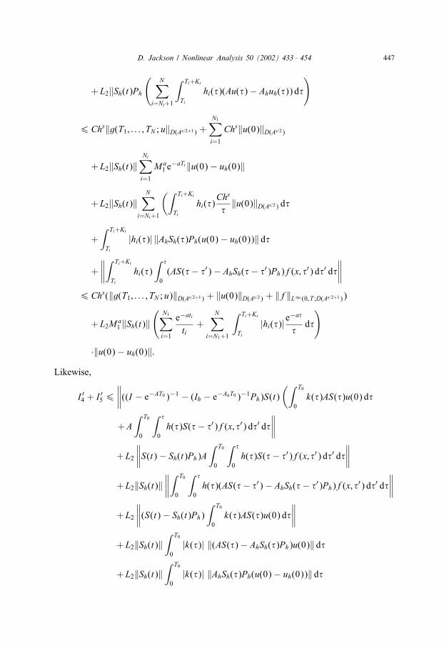
+L2‖Sh(t)Ph
(N∑
i=Ni+1
∫ Ti+Ki
Ti
hi(�)(Au(�)− Ahuh(�)) d�
)
6Chs‖g(T1; : : : ; TN ; u‖D(As=2+1) +N1∑i=1
Chs‖u(0)‖D(As=2)
+L2‖Sh(t)‖Ni∑i=1
Ma1 e
−aTi‖u(0)− uh(0)‖
+L2‖Sh(t)‖N∑
i=Ni+1
(∫ Ti+Ki
Ti
hi(�)Chs
�‖u(0)‖D(As=2) d�
+∫ Ti+Ki
Ti
|hi(�)| ‖AhSh(�)Ph(u(0)− uh(0))‖ d�
+∥∥∥∥∫ Ti+Ki
Ti
hi(�)∫ �
0(AS(�− �′)− AhSh(�− �′)Ph)f(x; �′) d�′ d�
∥∥∥∥6Chs(‖g(T1; : : : ; TN ; u)‖D(As=2+1) + ‖u(0)‖D(As=2) + ‖f‖L∞(0;T ;D(As=2+1))
+L2Ma1 ‖Sh(t)‖
(N1∑i=1
e−ati
ti+
N∑i=N1+1
∫ Ti+Ki
Ti
|hi(�)|e−a�
�d�
)
·‖u(0)− uh(0)‖:Likewise,
I ′4 + I ′56∥∥∥∥((I − e−AT0 )−1 − (Ih − e−AhT0 )−1Ph)S(t)
(∫ T0
0k(�)AS(�)u(0) d�
+A∫ T0
0
∫ �
0h(�)S(�− �′)f(x; �′) d�′ d�
∥∥∥∥+L2
∥∥∥∥S(t)− Sh(t)Ph)A∫ T0
0
∫ �
0h(�)S(�− �′)f(x; �′) d�′ d�
∥∥∥∥+L2‖Sh(t)‖
∥∥∥∥∫ T0
0
∫ �
0h(�)(AS(�− �′)− AhSh(�− �′)Ph)f(x; �′) d�′ d�
∥∥∥∥+L2
∥∥∥∥(S(t)− Sh(t)Ph)∫ T0
0k(�)AS(�)u(0) d�
∥∥∥∥+L2‖Sh(t)‖
∫ T0
0|k(�)| ‖(AS(�)− AhSh(�)Ph)u(0)‖ d�
+L2‖Sh(t)‖∫ T0
0|k(�)| ‖AhSh(�)Ph(u(0)− uh(0))‖ d�
448 D. Jackson / Nonlinear Analysis 50 (2002) 433– 454
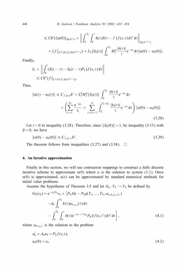
6Chs(‖u(0)‖D(As=2) +∥∥∥∥∫ T0
0
∫ �
0h(�)S(�− �′)f(x; �) d�′ d�
∥∥∥∥D(As=2+1)
+ ‖f‖L∞(0;T0;D(As=2+1)) + L2‖Sh(t)‖∫ T0
0Ma
1|k(�)|
�e−a� d�‖u(0)− uh(0)‖:
Finally,
I5 =∥∥∥∥∫ t
0(S(t − �)− Sh(t − �)Ph)f(x; �) d�
∥∥∥∥6Chs‖f‖L∞(0;T ;D(As=2+1)):
Thus,
‖u(t)− uh(t)‖6Cf; ;uhs + Lh1M
a1 ‖Sh(t)‖
∫ T0
0
|k(�)|�
e−a� d�
+
(N1∑i=1
e−ati
ti+
N∑i=N1+1
∫ Ti+Ki
Ti
|hi(�)|�
e−a� d�
)‖u(0)− uh(0)‖:
(3.28)
Let t=0 in inequality (3.28). Therefore, since ‖Sh(0)‖=1; by inequality (3.13) with*=0, we have
‖u(0)− uh(0)‖6Cf; ;fhs: (3.29)
The theorem follows from inequalities (3.27) and (3:38).
4. An iterative approximation
Finally in this section, we will use contraction mappings to construct a fully discreteiterative scheme to approximate u(0) where u is the solution to system (1.1). Onceu(0) is approximated, u(t) can be approximated by standard numerical methods forinitial value problems.Assume the hypotheses of Theorem 3:5 and let Gh :Vh → Vh be de�ned by
Gh(vh) = e−AhT0vh +[PhA − Phg(T1; : : : ; TN ; uh;Ah;vh;Af)
−Ah
∫ T0
0k(�)uh;vh; 0 (�) d�
−∫ T0
0
∫ �
0h(�)e−(�−�′)AhPhAf(x; �′) d�′ d�
]; (4.1)
where uh;vh;f is the solution to the problem
u′h + Ahuh =Phf(x; t);
uh(0)= vh: (4.2)
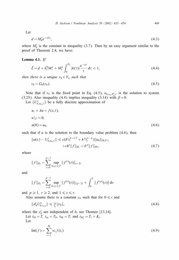
D. Jackson / Nonlinear Analysis 50 (2002) 433– 454 449
Let
d=M ′0e
−aT0 ; (4.3)
where M ′0 is the constant in inequality (3.7). Then by an easy argument similar to the
proof of Theorem 2.4, we have:
Lemma 4.1. If
2L=d+ k01Ma1 +Ma
1
∫ T0
0|k(�)|e
−a�
�d�¡ 1; (4.4)
then there is a unique vh ∈Vn such that
vh =Gh(vh): (4.5)
Note that if vh is the �xed point in Eq. (4.5), uh;vh;P1hf
is the solution to system(3.25). Also inequality (4.4) implies inequality (3.14) with *=0.
Let {Uih;u0 ;f} be a fully discrete approximation of
ut + Au=f(x; t);
u |� =0;
u(0)= u0; (4.6)
such that if u is the solution to the boundary value problem (4.6), then
‖u(ti)− Uih;u0 ;f‖6 c(hst%−s=2
i + kpt%−pi )‖u0‖D(A%)
+chs‖f‖H1 + kp‖f‖H2 ; (4.7)
where
‖f‖H1 =p−1∑i=0
sup06t6T
‖f(i)(t)‖s−2i
and
‖f‖H2 =p−1∑i=0
sup06t6T
‖f(i)(t)‖2p−2i +∫ T
0‖f(p)(s)‖ ds
and p¿ 1; r¿ 2; and 16 s6 r.Also assume there is a constant c0 such that for 06 i and
‖AihU
nh;vn; 0‖6 c0
tin‖vh‖; (4.8)
where the ci0 are independent of h, see Thomee [13,14].Let tM =T; tn0 =T0; tMi =Ti and tM ′
1=Ti + Ki.
Let
Int(f)=M∑i=1
wif(ti) (4.9)
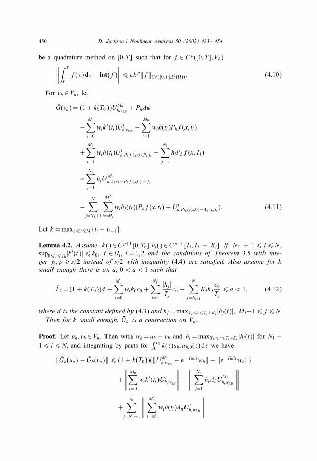
450 D. Jackson / Nonlinear Analysis 50 (2002) 433– 454
be a quadrature method on [0; T ] such that for f∈Cp([0; T ]; Vh)∥∥∥∥∫ T
0f(�) d�− Int(f)
∥∥∥∥6 ckp‖f‖Cp([0;T ];L2(�)): (4.10)
For vh ∈Vh, let
2G(vh) = (1 + k(T0))UM0h;vh;0
+ PhA
−M0∑i=0
wik ′(ti)Uih;vh;0 −
M0∑i=1
wih(ti)Phf(x; ti)
+M0∑i=1
wih(ti)Uih;Phf(x;0);Phft −
N1∑j=1
hiPhf(x; Ti)
−N1∑j=1
hiUMih;Ahvh−Phf(x;0);−ft
−N∑
j=N1+1
M ′j∑
i=Mj
wihj(ti)(Phf(x; ti)− Uih;Phfh(x;0)−Ahvh;ft ): (4.11)
Let k =max16i6M{ti − ti−1}.
Lemma 4.2. Assume k()∈Cp+1[0; T0]; hi()∈Cp+1[Ti; Ti + Ki] if N1 + 16 i6N ,sup06t6T0
|k ′(t)|6 k0; f∈Hi; i=1; 2 and the conditions of Theorem 3:5 with inte-ger p;p¿ s=2 instead of s=2 with inequality (4:4) are satis7ed. Also assume for ksmall enough there is an a; 0¡a¡ 1 such that
2L2 = (1 + k(T0))d+M0∑i=0
wik0c0 +N1∑j=1
|hj|Tj
c0 +N∑
j=Ni+1
Kjhjc0Tj6 a¡ 1; (4.12)
where d is the constant de7ned by (4:3) and hj =maxTj6t6Tj+Kj |hj(t)|; Mj+16 j6N .Then for k small enough, 2Gh is a contraction on Vh.
Proof. Let uh; vh ∈Vh. Then with wh = uh − vh and hi =maxT16t6Ti+Ki |hi(t)| for N1 +16 i6N; and integrating by parts for
∫ T0
0 k(�)uh; uh;0(�) d� we have
‖ 2Gh(un)− 2Gh(vn)‖6 (1 + k(T0))(‖UM0h;wh;0
− e−T0Ahwh‖+ ‖e−T0Ahwh‖)
+
∥∥∥∥∥M0∑i=0
wik ′(ti)Uih;wh;0
∥∥∥∥∥+∥∥∥∥∥
N1∑j=1
hiAhUMj
h;wh;0
∥∥∥∥∥+
N∑j=N1+1
∥∥∥∥∥M ′
i∑i=Mi
wih(ti)AhU ih;wh;0
∥∥∥∥∥
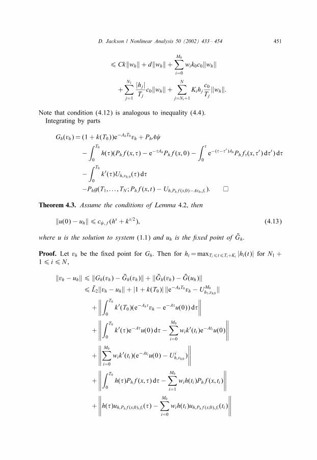
D. Jackson / Nonlinear Analysis 50 (2002) 433– 454 451
6Ck‖wh‖+ d‖wh‖+M0∑i=0
wik0c0‖wh‖
+N1∑j=1
|hj|Tj
c0‖wh‖+N∑
j=Ni+1
Kihjc0Tj
‖wh‖:
Note that condition (4.12) is analogous to inequality (4.4).Integrating by parts
Gh(vh) = (1 + k(T0))e−AhT0vh + PhA
−∫ T0
0h(�)(Phf(x; �)− e−�AhPhf(x; 0)−
∫ �
0e−(�−�′)AhPhf�(x; �′) d�′) d�
−∫ T0
0k ′(�)Uh;vh; 0 (�) d�
−Phg(T1; : : : ; TN ;Phf(x; t)− Uh;Phf(x;0)−Avh;ft ):
Theorem 4.3. Assume the conditions of Lemma 4:2; then
‖u(0)− uh‖6 c ;f(hs + ks=2); (4.13)
where u is the solution to system (1:1) and uh is the 7xed point of 2Gh.
Proof. Let vh be the �xed point for Gh. Then for hi =maxTi6t6Ti+Ki |hi(t)| for N1 +16 i6N ,
‖vh − uh‖6 ‖Gh(vh)− 2Gh(vh)‖+ ‖ 2Gh(vh)− 2G(uh)‖6 2L2‖vh − uh‖+ |1 + k(T0)| ‖e−AhT0vh − UM0
h1 ;vh;0‖
+∥∥∥∥∫ T0
0k ′(T0)(e−Ah�vh − e−A�u(0)) d�
∥∥∥∥+
∥∥∥∥∥∫ T0
0k ′(�)e−A�u(0) d�−
M0∑i=0
wik ′(ti)e−Ati u(0)
∥∥∥∥∥+
∥∥∥∥∥M0∑i=0
wik ′(ti)(e−Ati u(0)− Uih;vh;0 )
∥∥∥∥∥+
∥∥∥∥∥∫ T0
0h(�)Phf(x; �) d�−
M0∑i=1
wih(ti)Phf(x; ti)
∥∥∥∥∥+
∥∥∥∥∥h(�)uh;Phf(x;0);ft (�)−M0∑i=0
wih(ti)uh;Phf(x;0);ft (ti)
∥∥∥∥∥
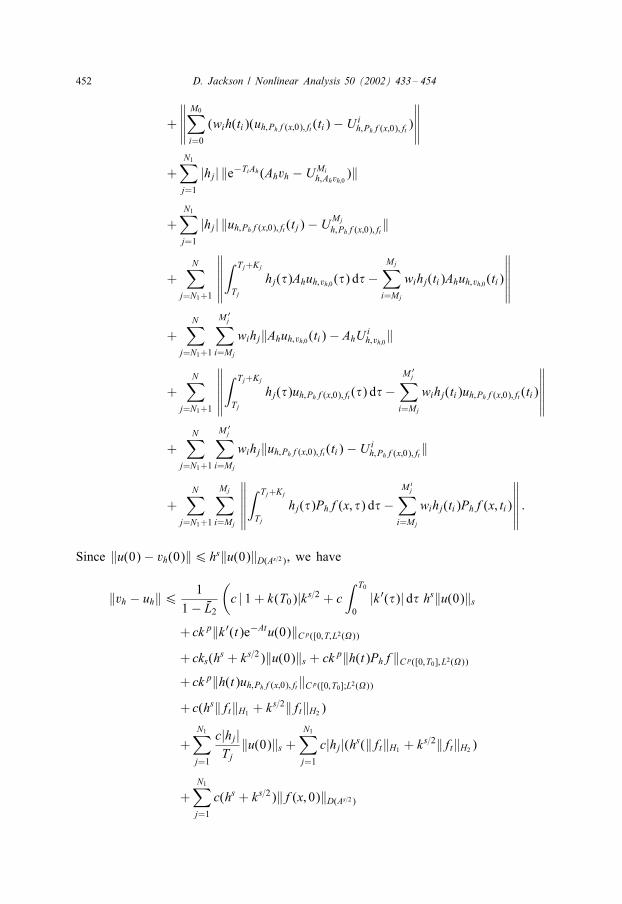
452 D. Jackson / Nonlinear Analysis 50 (2002) 433– 454
+
∥∥∥∥∥M0∑i=0
(wih(ti)(uh;Phf(x;0);ft (ti)− Uih;Phf(x;0);ft )
∥∥∥∥∥+
N1∑j=1
|hj| ‖e−TiAh(Ahvh − UMih;Ahvh;0
)‖
+N1∑j=1
|hj| ‖uh;Phf(x;0);ft (tj)− UMj
h;Phf(x;0);ft‖
+N∑
j=N1+1
∥∥∥∥∥∥∫ Tj+Kj
Tj
hj(�)Ahuh;vh;0 (�) d�−Mj∑
i=Mj
wihj(ti)Ahuh;vh;0 (ti)
∥∥∥∥∥∥+
N∑j=N1+1
M ′j∑
i=Mj
wihj‖Ahuh;vh;0 (ti)− AhU ih;vh;0‖
+N∑
j=N1+1
∥∥∥∥∥∥∫ Tj+Kj
Tj
hj(�)uh;Phf(x;0);ft (�) d�−M ′
j∑i=Mj
wihj(ti)uh;Phf(x;0);ft (ti)
∥∥∥∥∥∥+
N∑j=N1+1
M ′j∑
i=Mj
wihj‖uh;Phf(x;0);ft (ti)− Uih;Phf(x;0);ft‖
+N∑
j=N1+1
Mj∑i=Mj
∥∥∥∥∥∥∫ Tj+Kj
Tj
hj(�)Phf(x; �) d�−Mi
j∑i=Mj
wihj(ti)Phf(x; ti)
∥∥∥∥∥∥ :
Since ‖u(0)− vh(0)‖6 hs‖u(0)‖D(As=2), we have
‖vh − uh‖6 11− 2L2
(c | 1 + k(T0)|ks=2 + c
∫ T0
0|k ′(�)| d� hs‖u(0)‖s
+ ckp‖k ′(t)e−Atu(0)‖Cp([0;T;L2(�))
+ cks(hs + ks=2)‖u(0)‖s + ckp‖h(t)Phf‖Cp([0;T0]; L2(�))
+ ckp‖h(t)uh;Phf(x;0);ft‖Cp([0;T0];L2(�))
+ c(hs‖ft‖H1 + ks=2‖ft‖H2 )
+N1∑j=1
c|hj|Tj
‖u(0)‖s +N1∑j=1
c|hj|(hs(‖ft‖H1 + ks=2‖ft‖H2 )
+N1∑j=1
c(hs + ks=2)‖f(x; 0)‖D(As=2)
D. Jackson / Nonlinear Analysis 50 (2002) 433– 454 453
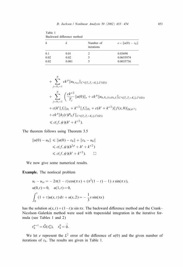
Table 1Backward diDerence method
h k Number of e= ‖u(0)− vh‖iterations
0.1 0.01 2 0.036980.02 0.02 5 0.06559740.02 0.001 5 0.0035736
+N∑
j=N1+1
ckp‖uh;vh;0‖Cp([Tj;Tj+Kj]; L2(�))
+N∑
j=N1+1
(cks=2
Tj‖u(0)‖s + ckp‖uh;Phf(x;0);ft‖Cp([Tj;Tj+Kj]; L2(�))
+ c(hs‖ft‖H1 + ks=2‖ft‖H2 + c(hs + ks=2)‖f(x; 0)|D(As=2)
+ ckp‖hj(t)Phf‖Cp([Tj;Tj+Kj]; L2(�))
6 c(f; )(hs + ks=2):
The theorem follows using Theorem 3:5
‖u(0)− uh‖6 ‖u(0)− vh‖+ ‖vh − uh‖6 c(f; )(h2p + hs + ks=2)
6 c(f; )(hs + ks=2):
We now give some numerical results.
Example. The nonlocal problem
ut − uxx =− 26(1− t) cos(6 x) + (62(1− t)− 1) x sin(6 x);
u(0; t)= 0; u(1; t)= 0;∫ 1
0(1 + �)u(x; �) d�+ u(x; 2)=− 1
3x sin(6x)
has the solution u(x; t)= (1−t)x sin 6x. The backward diDerence method and the Crank–Nicolson–Galerkin method were used with trapezoidal integration in the iterative for-mula (see Tables 1 and 2)
vn+1h = 2G(vnh); v0h =
*0 :
We let e represent the L2 error of the diDerence of u(0) and the given number ofiterations of vh. The results are given in Table 1.
454 D. Jackson / Nonlinear Analysis 50 (2002) 433– 454
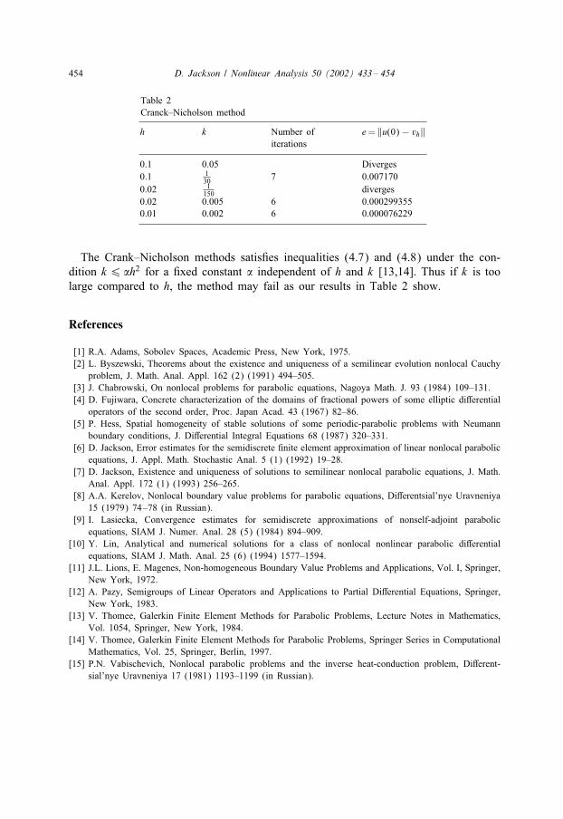
Table 2Cranck–Nicholson method
h k Number of e= ‖u(0)− vh‖iterations
0.1 0.05 Diverges0.1 1
30 7 0.0071700.02 1
150 diverges0.02 0.005 6 0.0002993550.01 0.002 6 0.000076229
The Crank–Nicholson methods satis�es inequalities (4.7) and (4.8) under the con-dition k6 %h2 for a �xed constant % independent of h and k [13,14]. Thus if k is toolarge compared to h, the method may fail as our results in Table 2 show.
References
[1] R.A. Adams, Sobolev Spaces, Academic Press, New York, 1975.[2] L. Byszewski, Theorems about the existence and uniqueness of a semilinear evolution nonlocal Cauchy
problem, J. Math. Anal. Appl. 162 (2) (1991) 494–505.[3] J. Chabrowski, On nonlocal problems for parabolic equations, Nagoya Math. J. 93 (1984) 109–131.[4] D. Fujiwara, Concrete characterization of the domains of fractional powers of some elliptic diDerential
operators of the second order, Proc. Japan Acad. 43 (1967) 82–86.[5] P. Hess, Spatial homogeneity of stable solutions of some periodic-parabolic problems with Neumann
boundary conditions, J. DiDerential Integral Equations 68 (1987) 320–331.[6] D. Jackson, Error estimates for the semidiscrete �nite element approximation of linear nonlocal parabolic
equations, J. Appl. Math. Stochastic Anal. 5 (1) (1992) 19–28.[7] D. Jackson, Existence and uniqueness of solutions to semilinear nonlocal parabolic equations, J. Math.
Anal. Appl. 172 (1) (1993) 256–265.[8] A.A. Kerelov, Nonlocal boundary value problems for parabolic equations, DiDerentsial’nye Uravneniya
15 (1979) 74–78 (in Russian).[9] I. Lasiecka, Convergence estimates for semidiscrete approximations of nonself-adjoint parabolic
equations, SIAM J. Numer. Anal. 28 (5) (1984) 894–909.[10] Y. Lin, Analytical and numerical solutions for a class of nonlocal nonlinear parabolic diDerential
equations, SIAM J. Math. Anal. 25 (6) (1994) 1577–1594.[11] J.L. Lions, E. Magenes, Non-homogeneous Boundary Value Problems and Applications, Vol. I, Springer,
New York, 1972.[12] A. Pazy, Semigroups of Linear Operators and Applications to Partial DiDerential Equations, Springer,
New York, 1983.[13] V. Thomee, Galerkin Finite Element Methods for Parabolic Problems, Lecture Notes in Mathematics,
Vol. 1054, Springer, New York, 1984.[14] V. Thomee, Galerkin Finite Element Methods for Parabolic Problems, Springer Series in Computational
Mathematics, Vol. 25, Springer, Berlin, 1997.[15] P.N. Vabischevich, Nonlocal parabolic problems and the inverse heat-conduction problem, DiDerent-
sial’nye Uravneniya 17 (1981) 1193–1199 (in Russian).


![arXiv:1109.0816v4 [math.AP] 2 Jan 2012arxiv.org/pdf/1109.0816.pdfarXiv:1109.0816v4 [math.AP] 2 Jan 2012 Lp-MAXIMAL REGULARITY OF NONLOCAL PARABOLIC EQUATION AND APPLICATIONS∗ XICHENG](https://static.fdocuments.us/doc/165x107/5f3f648dfc08093e7c56f68b/arxiv11090816v4-mathap-2-jan-arxiv11090816v4-mathap-2-jan-2012-lp-maximal.jpg)