Iterative Estimation, Equalization

and Decoding

A ThesisPresented to

The Academic FacultyBy

Renato da Rocha Lopes

In Partial Fulfillment of the Requirements for the

Degree of Doctor of Philosophy in Electrical Engineering

School of Electrical and Computer Engineering

Georgia Institute of Technology

July 8, 2003

Copyright 2003 by Renato da Rocha Lopes

NI•AIGR

OE

G•E

HT

•F

O •L A E S •

S T I T U T E• O

F•

TE

CH

NO

LOGY•

8 581

NA DPR O G R ESS S ER V I C E

Iterative Estimation, Equalization

and Decoding

Approved:

_____________________________________John R. Barry, Chairman

_____________________________________Steven W. McLaughlin

_____________________________________Aaron Lanterman

Date Approved _________________

iii

To my beloved wife Túria,

with my endless gratitude, love and admiration.

iv

Acknowledgments

First, I would like to thankDr. JohnBarry for his guidanceduringmy stayat Georgia

Tech.His very clearandobjective view of technicalmatters,aswell ashis deepinsights,

have influenceda lot my view of researchin telecommunications,andhopefullymadethis

work more clear and objective.

I would alsolike to thankDrs. LantermanandMcLaughlin for their constructive and

timely feedbackon my thesis,andDrs. Stüber andWang for beingpart of my defense

committee.

I am gratefulfor the help of the Schoolof ElectricalandComputerEngineering:Dr.

Sayle,Dr. Hertling,Marilou andotherswerealwaystherewhenneeded.Also, I would like

to thanktheSchoolof ECE,CRASPandtheBraziliangovernment,throughCAPES,for

their financial support during different stages of this program.

I amdeeplyindebtedto my wife, Túria, for hersupport,love andencouragement,and

for having pushedmewhenI neededpushing.I considermyselfblessedto bemarriedto

sucha wonderful person.Without her, this work and a lot more would not have been

possible. For all she has done and put up with, I dedicate this thesis to her.

v

I would alsolike to thankmy parentsfor their unconditionalsupportandlove. They

have alwaystaughtmetheimportanceof a positive attitude,andhow learningcanbefun.

Theselessons,and their unshakablebelieve in me, have beenvery important for the

completion of my studies.

I am also grateful to my parents-in-law, who have shown great patience and faith.

Thanksarealsoin orderto all thefolks at GCATT: Mai, Estuardo,Andrew, Elizabeth,

Jau,Apu, Aravind, Badri,Ana,Ravi, Kofi, Chen-Chu,Ricky, Babak,Cagatai,andthelist

could go on forever. These incredible people showed me how vast the area of

telecommunicationsis, and helpedme have a deeperunderstandingof many research

questions.And thediscussionswith themaboutmusic,cooking,religion,politics,cricket,

etc.,greatlybroadenedmy horizons.They helpedmake thisexperienceall themoreworth

it.

Finally, thereis the Brazilian crowd of Atlanta,who provided delightful breaksfrom

thedaily strugglesof thePh.D.program,andfrom theoccasionalstruggleof life abroad:

Ânderson,Mônica, Pedro, Jackie, Sharlles,Adriane, Henrique, Sônia, Augusto, the

musicians, and many others.Valeu!

vi

Table of Contents

Acknowledgments iv

Table of Contents vi

List of Figures ix

Summary xii

1 Introduction 1

2 Problem Statement and Background 11

2.1 Problem Statement .................................................................................................11

2.2 Turbo Equalization.................................................................................................14

2.2.1 The BCJR Algorithm ...................................................................................16

2.3 Blind Iterative Channel Estimation with the EM Algorithm.................................19

3 A Simplified EM Algorithm 24

3.1 Derivation of the SEM Algorithm .........................................................................24

3.2 Analysis of the Scalar Channel Estimator .............................................................27

3.3 The Impact of the Estimated Noise Variance ........................................................34

3.4 Simulation Results .................................................................................................35

3.5 Summary ................................................................................................................36

vii

4 The Extended-Window Algorithm (EW) 37

4.1 A Study of Misconvergence...................................................................................37

4.2 The EW Channel Estimator...................................................................................39

4.2.1 Delay and Noise Variance Estimator............................................................40

4.3 Simulation Results.................................................................................................41

4.4 Summary................................................................................................................47

5 The Soft-Feedback Equalizer 49

5.1 Previous Work on Interference Cancellation.........................................................50

5.2 The Soft-Feedback Equalizer.................................................................................52

5.2.1 The SFE Coefficients....................................................................................53

5.2.2 Computing the Expected Values..................................................................55

5.2.3 Special Cases and Approximations..............................................................58

5.3 Performance Analysis............................................................................................61

5.4 Summary................................................................................................................63

6 Turbo Equalization with the SFE 65

6.1 An SFE-Based Turbo Equalizer.............................................................................66

6.2 Simulation Results.................................................................................................68

6.3 The EXIT Chart.....................................................................................................76

6.4 Summary................................................................................................................81

7 ECC-Aware Blind Channel Estimation 82

7.1 ECC-Aware Blind Estimation of a Scalar Channel...............................................82

7.2 ECC-Aware Blind Estimation of an ISI Channel..................................................83

viii

7.3 Simulation Results .................................................................................................86

7.4 Study of Convergence............................................................................................88

7.5 Initialization ...........................................................................................................91

7.6 Turbo Estimator .....................................................................................................94

7.7 Summary ................................................................................................................96

8 Conclusions 97

8.1 Summary of Contributions.....................................................................................97

8.2 Directions for Future Research ............................................................................100

A Computing Hard Scalar-Channel Estimates 102

B Computing the SFE Coefficients 105

References 108

VITA 115

ix

List of Figures

1 Blind iterative channel estimation...............................................................................7

2 Channel model...........................................................................................................11

3 Turbo equalizer..........................................................................................................14

4 The EM algorithm for blind iterative channel estimation.........................................23

5 Blind iterative channel estimation with the SEM algorithm.....................................26

6 Estimated relative channel reliabilityαi as a function of its value in the previous iter-ation,αi–1. .........................................................................................................................30

7 Tracking the trajectories of the EM and the SEM estimators for a scalar channel...32

8 Asymptotic error of gain estimates as a function of SNR. Dashed lines correspond totheoretical predictions, solid lines correspond to a simulation with 106 transmitted bits.33

9 Asymptotic error of noise variance estimates as a function of SNR. Dashed lines cor-respondto theoreticalpredictions,solid linescorrespondto asimulationwith 106 transmit-ted bits...............................................................................................................................33

10 Performancecomparison:channelandnoisestandarddeviationestimatesasafunctionof iteration for EM (light solid) and simplified EM (solid) algorithms. Actual parametersare also shown (dotted).....................................................................................................35

11 Frequency response ofh = [–0.2287, 0.3964, 0.7623, 0.3964, –0.2287]..................42

12 Estimatesof h = [–0.2287,0.3964,0.7623,0.3964,–0.2287],producedby theextend-ed-window algorithm........................................................................................................42

13 EM estimates ofh = [–0.2287, 0.3964, 0.7623, 0.3964, –0.2287]............................43

14 Estimates ofσ2, produced by the extended-window algorithm................................43

15 Estimationerrorfor thechannelprobing,MMSE, EM andEW estimatesafter20 iter-

x

ations. ................................................................................................................................44

16 Bit error rate using the trained, EM and EW estimates after 20 iterations. ...............45

17 WER for the EW and the EM algorithms for an ensemble of 1,000 random channels. 46

18 Histograms of estimation errors for the EW and the EM algorithms over an ensembleof 1,000 random channels. ................................................................................................46

19 Interference canceller with a priori information. .......................................................50

20 The proposed SFE equalizer. The thicker line in the feedback loop represents the onlyactual change from Fig. 19. ...............................................................................................53

21 Graphical analysis of the convergence of (72), (73): estimated value of γei+1 as a func-

tion of its value at the previous iteration, γei . ....................................................................57

22 The behavior of ψ1(γ), ψ1(γ)/ψ2(γ), and ψ12(γ)/ψ2(γ). ..............................................58

23 Estimated pdf of the SFE output, compared to the pdf of the LLR of an AWGN chan-nel. ....................................................................................................................................61

24 BER (theoretical and simulation) of an SFE with no a priori information. The BER ofa DFE is also shown. .........................................................................................................62

25 Turbo equalizer. .........................................................................................................65

26 An SFE-based turbo equalizer. ..................................................................................66

27 Frequency response of h = [0.227, 0.46, 0.688, 0.46, 0.227]. ...................................69

28 BER performance for the simulation scenario of [35]. ..............................................70

29 Complexity-performance trade-off. ...........................................................................71

30 Frequency response of h = [0.23, 0.42, 0.52, 0.52, 0.42, 0.23]. ................................72

31 BER performance of some turbo equalizers for h = [0.23, 0.42, 0.52, 0.52, 0.42, 0.23].The BPSK capacity limit for this scenario is Eb/N0 = 4.2 dB. .........................................73

32 Impulse response of microwave channel of [49]. ......................................................74

33 Frequency response of microwave channel of [49]. ..................................................75

34 BER performance of the SFE- and SE-based turbo equalizers for the microwave chan-nel. ....................................................................................................................................76

xi

35 View of turbo equalization as an iterative application of mappings. ........................77

36 The EXIT charts for the BCJR equalizer, the SFE and the SE at Eb/N0 = 5.1 dB andfor h = [0.227, 0.46, 0.688, 0.46, 0.227]. The flipped decoder chart is also shown. ........78

37 A simple encoded scalar channel. ..............................................................................83

38 Integrating channel estimation with turbo equalization. ............................................84

39 Comparison between ECC-aware blind channel estimation and channel knowledge inturbo equalization. .............................................................................................................87

40 Comparison between ECC-aware and ECC-ignorant blind channel estimation. ......88

41 Word-error rate (WER) across different channels. ....................................................90

42 Comparison between CMS and ECC-aware blind channel estimates. ......................92

43 WER for different initialization strategies. ................................................................93

44 Channel estimation errors for the SFE-based ECC-aware blind channel estimator. .95

45 BER performance of the SFE-based ECC-aware blind channel estimator. ...............95

xii

Summary

Knowledgeof thechannelis valuablefor equalizerdesign.To estimatethechannel,a

training sequence,known to the transmitterand the receiver, is normally transmitted.

However, transmissionof a training sequencedecreasesthe systemthroughput.Blind

channelestimationusesonly the statisticsof the transmittedsignal.Thus,it requiresno

training sequence, increasing the throughput.

Most real-lifecommunicationsystemsemploy someform of error-controlcode(ECC)

to improve the systemperformanceundernoise.In fact, with the advent of turbo codes

and turbo equalization,reliable transmissionat a signal to noise ratio (SNR) close to

capacityis now feasible.However, blind estimatorsthat ignorethe codemay fail at low

SNR.Recently, blind estimatorshave beenproposedthatexploit theECCandwork well

at low SNR. Thesealgorithms are inspired by turbo equalizersand the expectation-

maximization (EM) channel estimator.

The objective of this researchis to develop a low-complexity ECC-aware blind

channelestimator. We first proposethe extended-window (EW) algorithm, a channel

estimator that is less complex than the EM estimator, and has better convergence

properties.Furthermore,the EM algorithm usesthe computationallycomplex forward-

backwardrecursion(BCJRalgorithm)for symbolestimation.With theEW estimator, any

soft-output equalizer may be used, allowing for further complexity reduction.

xiii

We then proposethe soft-feedbackequalizer(SFE), a low-complexity soft-output

equalizerthatcanusea priori informationon thetransmittedsymbols,andis thussuitable

for turbo equalization.The coefficients of the SFE are chosento minimize the mean-

squarederror betweenthe equalizeroutputandthe transmittedsymbols,anddependon

the“quality” of thea priori informationandtheequalizeroutput.Simulationresultsshow

that the SFE may perform within 1 dB of a system using a BCJR equalizer, and

outperforms other schemes of comparable complexity.

Finally, we show how theSFEandtheEW algorithmsmaybecombinedto form the

turbo estimator(TE), a linear-complexity ECC-awareblind channelestimator. We show

that theTE performscloseto systemswith channelknowledgeat low SNR,whereECC-

ignorant channel estimators fail.

1

CHAPTER 1

Introduction

Error-controlcodes(ECC),or channelcodes,allow for reliabletransmissionof digital

information in the presenceof noise. Through this process,an information-bearing

sequenceof lengthK, calleda message, is mapped,or encoded,into anothersequenceof

lengthN > K, calledacodeword. Thisencodingintroducesredundancy, but it alsorestricts

the numberof possibletransmittedcodewords,allowing for reliablecommunicationat a

lower signal-to-noiseratio (SNR) [1]. The codeword is thenmodulatedand transmitted

throughthe communicationschannel.The received signal is a distortedversionof the

modulatedcodeword; in particular, communicationschannelsintroducenoise,normally

modeledasadditive white Gaussiannoise(AWGN), and intersymbolinterference(ISI),

the effects of which are normally modeled by a linear filter.

Thereceivergoalcanbeveryclearlyandconciselydescribed:thetransmittedmessage

bitsshouldbeestimatedat thereceiveraccordingto a rule thatminimizesthebit errorrate

(BER). Assuming equally likely messagebits, this rule can be implementedwith a

maximum-likelihood(ML) detector, which estimateseachmessagebit soasto maximize

the likelihood of observing the received signal conditioned on the message bit [1].

2

ML detectorsjointly andoptimallyperformall receiver tasks,suchassynchronization,

timing recovery, channel estimation, equalization, demodulation and decoding.

Unfortunately, the computationalcomplexity of ML receivers is prohibitive. In some

cases,such as codedsystemswith interleavers, an ML receiver has to considerevery

possible transmittedmessageindependently. For messagesof 1,000 bits, this means

considering21,000 messages,much more than the current estimatefor the numberof

atomsin the universe[2]. Until the promiseof quantumcomputers(which theoretically

could analyzeall possiblemessagessimultaneously)is realized [3], or until a better

strategy is discovered,exact ML detectionwill remain a benchmarkand an object of

theoretical investigation.

Traditionally, receivers employ a suboptimal divide-and-conquerapproach for

recoveringthetransmittedmessagefrom thereceivedsignal.First, timing is estimated[1]

andthesignalis sampled.Thentheequalizerparametersareestimated[1,4-8]. After that,

theequalizerremovestheISI introducedby thechannel[1], sothat its outputcanbeseen

asa noise-corruptedversionof the transmittedcodeword. Finally, theequalizeroutputis

fed to the channeldecoderwhich, exploiting the beneficialeffectsof channelencoding,

estimates the transmitted message [2].

The divide-and-conquerapproachis clearly suboptimal.Consider, for instance,the

problemof channelestimation.Traditionally, the channelis estimatedby transmittinga

known sequence,called a training sequence[1,4,5], and the received samples

correspondingto the training sequenceareusedfor estimation.However, this approach,

known as trained estimation,ignoresreceived samplescorrespondingto the information

bits, and thus doesnot use all the information available at the receiver. To improve

3

performance,the channelmay be estimatedbasedon all received samples,in what is

known assemi-blind estimation[6]. Channelestimationis still possibleevenif no training

sequenceis available. In this case,we obtain blind channel estimates[7,8]. When

performing blind or semi-blind channel estimation under the divide-and-conquer

framework, the fact that the transmittedsignal is restrictedto be a codeword of a given

channel code is not exploited. However, it seemsclear that performancewould be

improved if the channel encoding were taken into account.

In this work, we proposethe blind turbo estimator (TE), a low computational

complexity techniquefor exploiting thepresenceof ECCin blind andsemi-blindchannel

estimation. This work has four facets: channel estimation, blind and semi-blind

techniques,the exploitation of ECC,andlow computationalcomplexity. The importance

of each facet is discussed below:

• Channelestimation. Channelestimatesarerequiredby theML equalizer, andcan

beusedto computethecoefficientsof suboptimalbut lower-complexity equalizers

suchastheminimummean-squarederror(MMSE) linearequalizer(LE) [1], or the

MMSE decision-feedbackequalizer(DFE) [1]. Even thoughthe MMSE-LE and

theMMSE-DFEcanbeestimateddirectly, having thechannelestimatesallows us

to choosewhich equalizeris more appropriatefor the channel.For instance,in

channels with deep spectral nulls, DFE is known to perform better than LE.

• Blind and semi-blind techniques. By using every available channeloutput for

channelestimation,semi-blindtechniquesperform better than techniquesbased

solelyon thechanneloutputscorrespondingto trainingsymbolsandthuscanusea

shortertrainingsequence[6]. Therefore,semi-blindandblind techniquesincrease

4

thethroughputof a systemby requiringa small trainingsequenceor nonewhatso-

ever. Eavesdroppingis anotherapplicationof blind channelestimation.Theeaves-

droppermaynotknow whatthetrainingsequenceis andhencehasto rely onblind

estimation techniques.

• Exploitation of ECC. Most of the existing blind channelestimationtechniques

operatewithin thedivide-and-conquerframework, ignoring thepresenceof ECC,

andnormally assumingthat the transmittedsymbolsare independentand identi-

cally distributed (iid). This approachworks well at high signal-to-noiseratio

(SNR). However, the last decadehasseenthe discovery of powerful ECC tech-

niquessuchas turbo codesand low-densityparity checkcodes[9-11] that, with

reasonablecomplexity, allow reliabletransmissionat an SNR only fractionsof a

dB from channelcapacity. Whenpowerful codesareusedandsystemsoperateat

low SNR,blind andsemi-blindestimationtechniquesthatignoreECCaredoomed

to fail. This observationmotivatedthestudyof blind ECC-awarechannelestima-

tors in [12-17].

• Low computationalcomplexity. The per-symbol computationalcomplexity of

existing ECC-awarechannelestimatorsis exponentialin thememoryof thechan-

nel. However, in applicationssuchasxDSL andhigh-densitymagneticrecording,

the channelimpulsecanhave tensor even hundredsof coefficients.For channels

with long memory, existing ECC-awarechannelestimatorsareprohibitively com-

plex, which motivates the study of low-complexity techniques.

5

Examplesaboundthat show that it is possibleto improve the performanceof the

divide-and-conquerapproachsimply by having the receiver componentscooperate

throughan iterative exchangeof information. For instance,in turbo equalizers[18,19]

(whichassumechannelknowledge),thedecoderoutputis usedby theequalizerasa priori

informationon thetransmittedsymbols.Thisproducesimprovedequalizeroutputs,which

in turn produceimproveddecoderoutputs,andsoon. By iteratingbetweentheequalizer

andthedecoder, turboequalizersachieveaBERmuchsmallerthanthatof thedivide-and-

conquerapproach,with reasonablecomplexity. Iterative channelestimators[6,20-28]are

anotherimportantclassof iterative algorithmsthat performbetterthantheir noniterative

counterparts.In thesealgorithms,aninitial channelestimateis usedby asymbolestimator

to provide tentative estimatesof thefirst- and/orsecond-orderstatisticsof thetransmitted

symbol sequence.Thesestatisticsare then usedby a channelestimatorto improve the

channelestimates.Theimprovedchannelestimatesarethenusedby thesymbolestimator

to improve the estimates of the statistics, and so on.

Turbo equalizersand iterative channelestimatorsnormally rely on the forward-

backwardalgorithmby Bahl,Cocke,JelinekandRaviv (BCJR)[29] for equalization.This

algorithmcomputesthe a posteriori probabilities(APP) of the channelinputsgiven the

channeloutput,channelestimates,anda priori probabilitieson the channelinputs,and

assumingthat the channelinputsare independent.In otherwords,if an ECC is present,

this presence is ignored.

The BCJRalgorithmis well-suitedfor iterative systems,sinceit canusethe a priori

information at its input to improve the quality of its output and sinceit computessoft

symbolestimatesin theform of APP. However, its per-symbolcomputationalcomplexity

6

increasesexponentiallywith the channelmemory, andhenceis prohibitive for channels

with a long impulseresponse.This hasmotivatedthedevelopmentof reduced-complexity

alternatives to the BCJR algorithm, such as the equalizersproposedin [30-38]. The

structuresproposedin [30-35] usea linear filter to equalizethe received sequence.The

output of this filter containsresidual ISI, which is estimatedbasedon the a priori

information, and then cancelled.Reduced-statealgorithmsare investigated in [36-38];

however, these are more complex than the structures based on linear filters.

In this work, we propose the soft-feedback equalizer (SFE), a low-complexity

alternative to theBCJRalgorithmbasedon filters that is similar to thoseproposedin [30-

35]. Oneimportantdifferenceis thattheSFEusesastructuresimilar to aDFE,combining

the equalizeroutputsand a priori information to form more reliable estimatesof the

residualISI. A similar systemis proposedin [35] thatusesharddecisionson theequalizer

outputto estimatetheresidualISI. However, becauseharddecisionsareusedandbecause

the equalizeroutput is not combinedwith the a priori information beforea decisionis

made, the DFE-like system of [35] performs worse than schemes without feedback.

As in [32-35], theSFEdoesnot rely solelyon interferencecancellation(IC). Instead,

the SFE coefficients are computedso as to minimize the mean-squarederror (MSE)

between the equalizer output and the transmitted symbol. The resulting equalizer

coefficientsdependon thequality of theequalizeroutputandthea priori information.By

assuminga statisticalmodel for the equalizeroutputsand the a priori information,we

obtaina linear-complexity, time-invariantequalizer. In contrast,the MMSE structuresin

[32-35] have to becomputedfor every symbol,resultingin a per-symbolcomplexity that

7

is quadraticin the lengthof the equalizer. A similar statisticalmodel is usedin [39] to

obtain a time-invariant, linear-complexity, hard-input hard-outputequalizer with ISI

cancellation.

We will seethat in specialcases,theSFEreducesto anMMSE-LE, anMMSE-DFE,

or an IC. We will show that the SFE performsreasonablywell when comparedto the

BCJRalgorithmandthequadraticcomplexity algorithmsin [32-35],while it outperforms

other structures of comparable complexity proposed in the literature.

Iterative channelestimatorsfit theiterative paradigmdepictedin Fig. 1. In this figure,

a symbol estimatorproducessoft information on the transmittedsymbolsbasedon the

channelestimates, , and the noise varianceestimate, , provided by the channel

estimator. Thechannelestimatorthenusesthesoft informationonthetransmittedsymbols

to computeimprovedchannelestimates.Thenew channelestimatesarethenusedby the

symbol estimatorto computebetter soft information, and so on. The most important

iterative estimator, on which mostotheriterative estimatorsarebased,is theexpectation-

maximization(EM) algorithm[40,41]. In this algorithm,thesymbolestimatorin Fig. 1 is

basedon the BCJRalgorithmandproducessoft estimatesof the first- andsecond-order

statistics of the transmitted symbols.

Fig. 1. Blind iterative channel estimation.

h σ,

SYMBOLESTIMATOR

CHANNELESTIMATOR

h σ2

8

The EM algorithm has two sources of complexity. First, it involves the computation

and inversion of a square matrix whose order is equal to the channel length. Second, and

most important, it uses the BCJR algorithm for equalization. In this work, we will obtain a

simplified EM (SEM) algorithm that avoids the matrix inversion without significantly

affecting performance, resulting in a complexity that is proportional to the channel length.

More interestingly, based on the SEM, the soft symbol estimator may be implemented

with any of a number of low-complexity alternatives to the BCJR algorithm, such as the

SFE. Low complexity alternatives to the EM channel estimator are also proposed in

[25,26]. However, in these strategies the complexity is reduced through the use of a low-

complexity alternative to the BCJR algorithm. Therefore, they are intrinsically tied to an

equalization scheme. Furthermore, the estimators proposed in [25,26] do not avoid the

matrix inversion, resulting in a quadratic computational complexity.

In this work, we will also investigate convergence issues regarding iterative channel

estimators. The EM algorithm generates a sequence of estimates with nondecreasing

likelihood. Hence, the EM estimates may converge to the ML solution. However, they may

also get trapped in a nonglobal local maximum of the likelihood function. We will propose

a simple modification, called the extended-windowEM (EW) algorithm, which greatly

decreases the probability of misconvergence without significantly increasing the

computational complexity.

Finally, by viewing a turbo equalizer as a soft symbol estimator, we combine turbo

equalization with iterative channel estimation. Since turbo equalizers provide soft symbol

estimates that benefit from the presence of channel coding, the resulting turbo estimation

scheme is an ECC-aware channel estimator. Thus, we have proposed the turbo estimator

9

(TE), a linear complexity blind channel estimator that benefits from the presence of

channel coding. Other ECC-aware channel estimators were proposed [12-16], but they are

all based on the EM algorithm and hence suffer all the complexity and convergence

problems mentioned above.

To summarize, the main contributions of this work are:

• The soft-feedback equalizer (SFE), a linear complexity equalizer that produces

soft symbol estimates and benefits from a priori information at its input.

• The simplified EM (SEM) algorithm, an iterative channel estimator that is less

complex than the EM algorithm and is not intrinsically tied to the BCJR equalizer,

which opens the door for further complexity reduction.

• The extended window (EW) algorithm, an iterative channel estimator that is less

prone to misconvergence than the EM algorithm.

• The turbo estimator (TE), an iterative channel estimator that benefits from the

presence of ECC to produce reliable channel estimates at low SNR.

This thesis is organized as follows. In Chapter 2, we present the channel model and

describe the problem we will investigate, and provide some background material on turbo

equalization and iterative channel estimation via the EM algorithm. In Chapter 3, we

propose the SEM, a channel estimator that is less complex than the EM algorithm. In

Chapter 4, we propose the EW algorithm, an extension to the SEM algorithm that makes it

is less likely than the EM to get trapped in a local maximum of the joint likelihood

function. In Chapter 5, we propose the SFE, a linear-complexity alternative to the BCJR

equalizer. In Chapter 6, we describe the application of the SFE to turbo equalization.

10

Please note that Chapters 5 and 6 are not related to Chapters 3 and 4. In Chapter 7, we

propose the TE, a linear complexity ECC-aware channel estimator that combines the EW

algorithm of Chapter 4 with the SFE-based turbo equalizer of Chapter 6. In Chapter 8 we

summarize the contributions of this thesis and present directions for future work.

11

CHAPTER 2

Problem Statement and Background

In this chapter, we describe the model we will use for the communications system and

define the problem investigated in this research. We also provide background material on

two iterative techniques that solve parts of this problem: turbo equalization and iterative

channel estimation.

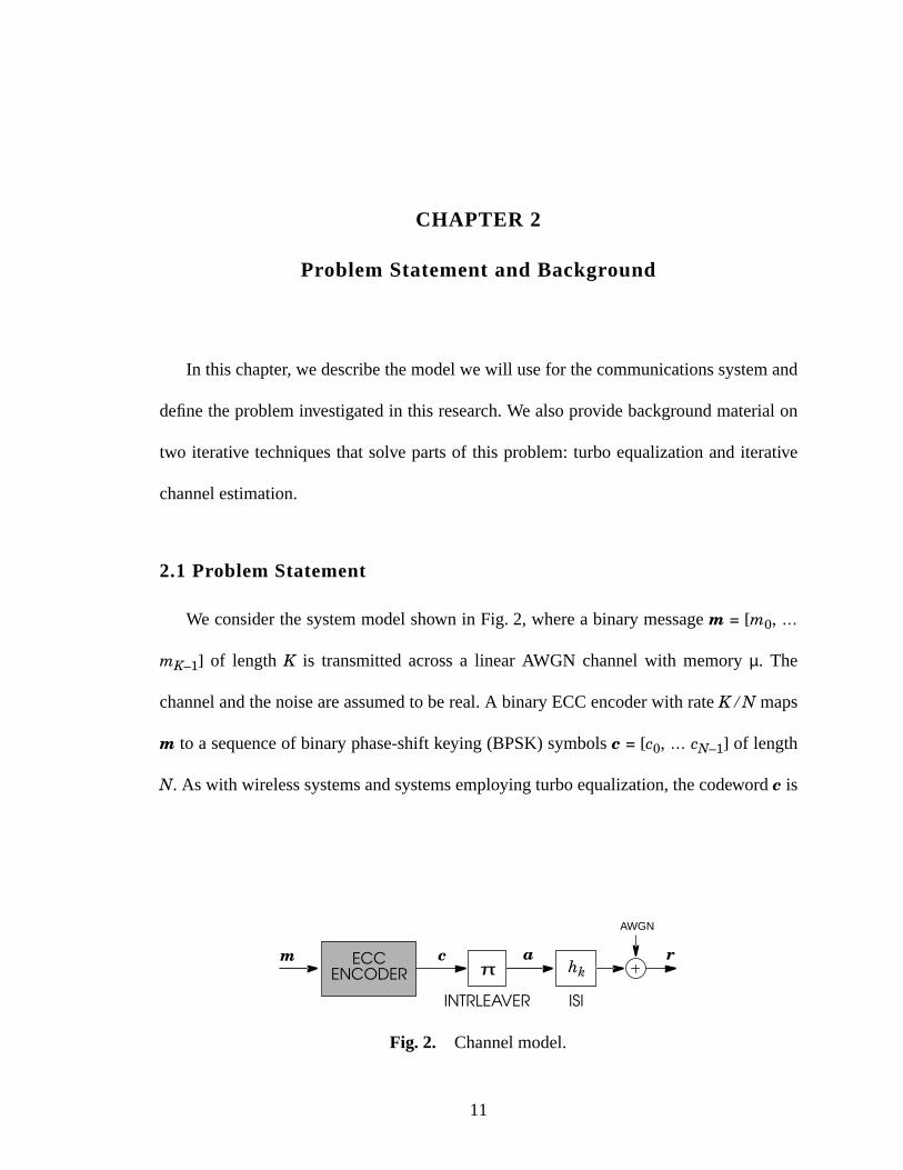
2.1 Problem Statement

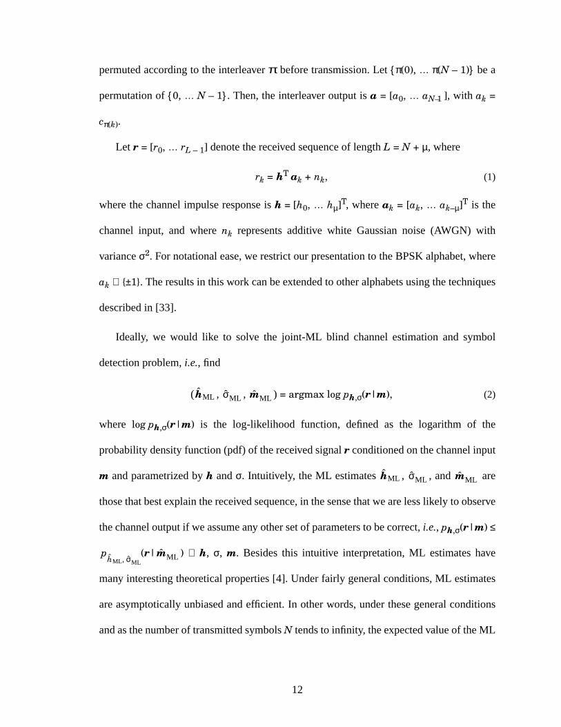
We consider the system model shown in Fig. 2, where a binary message m = [m0, …

mK–1] of length K is transmitted across a linear AWGN channel with memory µ. The

channel and the noise are assumed to be real. A binary ECC encoder with rate K ⁄ N maps

m to a sequence of binary phase-shift keying (BPSK) symbols c = [c0, … cN–1] of length

N. As with wireless systems and systems employing turbo equalization, the codeword c is

Fig. 2. Channel model.

ISI

hkm a r

πECC

INTRLEAVER

AWGN

ENCODERc

12

permuted according to the interleaver π before transmission. Let {π(0), … π(N – 1)} be a

permutation of {0, … N – 1}. Then, the interleaver output is a = [a0, … aN–1 ], with ak =

cπ(k).

Let r = [r0, … rL – 1] denote the received sequence of length L = N + µ, where

rk = hT ak + nk, (1)

where the channel impulse response is h = [h0, … hµ]T, where ak = [ak, … ak– µ]T is the

channel input, and where nk represents additive white Gaussian noise (AWGN) with

variance σ2. For notational ease, we restrict our presentation to the BPSK alphabet, where

ak ∈ {±1}. The results in this work can be extended to other alphabets using the techniques

described in [33].

Ideally, we would like to solve the joint-ML blind channel estimation and symbol

detection problem, i.e., find

( , , ) = argmax log ph,σ(r|m), (2)

where log ph,σ(r|m) is the log-likelihood function, defined as the logarithm of the

probability density function (pdf) of the received signal r conditioned on the channel input

m and parametrized by h and σ. Intuitively, the ML estimates , , and are

those that best explain the received sequence, in the sense that we are less likely to observe

the channel output if we assume any other set of parameters to be correct, i.e., ph,σ(r|m) ≤

(r| ) ∀ h, σ, m. Besides this intuitive interpretation, ML estimates have

many interesting theoretical properties [4]. Under fairly general conditions, ML estimates

are asymptotically unbiased and efficient. In other words, under these general conditions

and as the number of transmitted symbols N tends to infinity, the expected value of the ML

hML σML mML

hML σML mML

phML σML,

mML

13

estimatestendsto the actualvalueof the parameters,while the varianceof the estimates

tendsto theCramér-Raobound,which is the lowestvarianceachievableby any unbiased

estimator.

Unfortunately, the computational complexity of finding the ML estimates is

prohibitive. In this work, we will study iterative approachesthat provide approximate

solutions to the maximization problem in (2). The reasonfor the focus on iterative

approachesis that iterative techniquessuccessfullyprovide approximateML solutionsto

otherwise intractable problems, such as the following:

• On a codedsystemwith channelknowledge, turbo equalizersproducea good

approximation,with reasonablecomputationalcomplexity, to themaximizationof

log p(r|m).

• On an uncodedsystem,the EM algorithm provides a simple approximateML

channel estimate for the blind ECC-ignorant problem of maximizing

log ph,σ(r|a). Here, a is not restrictedto be a permutationof a codeword, but

instead can be any vector of symbols of lengthN.

Thesetechniquesareformulatedin a framework that makesit almoststraightforward to

combinethemin a moregeneraliterative algorithmthat performschannelidentification

and decoding, as we will see in chapter7.

One key ingredient of a successfuliterative algorithm is the use of soft symbol

estimatesin theform of APP’s.For a generalalphabetA, theAPPis a functionfrom A to

the interval [0,1] givenby Pr(ak = a|r), for a ∈ A. For a BPSKconstellation,theAPPis

fully captured by what is loosely referred to as the log-likelihood ratio (LLR), defined as

14

Lk = log . (3)

TheLLR hassomeinterestingproperties.For a BPSKalphabet,thesignof Lk determines

the maximuma posteriori (MAP) estimateof ak, which minimizesthe probability of a

decisionerror, and its magnitudeprovides a measureof the reliability of the decision.

Furthermore,Lk can be usedto obtain the MMSE estimateof ak, which, for a BPSK

alphabet, is given bytanh(Lk / 2).

Unfortunately, exact evaluationof the APP is computationallyhard.In the next two

sections,wewill briefly review turboequalizersandtheEM algorithm,whichareiterative

techniquesthat addresssimpler problemsand are the building blocks for the system

proposed in this work.

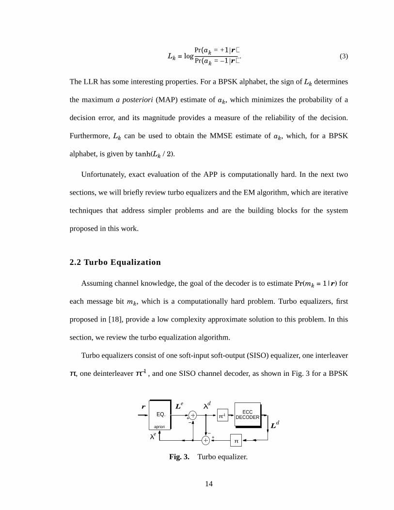
2.2 Turbo Equalization

Assumingchannelknowledge,thegoalof thedecoderis to estimatePr(mk = 1|r) for

eachmessagebit mk, which is a computationallyhard problem.Turbo equalizers,first

proposedin [18], provide a low complexity approximatesolutionto this problem.In this

section, we review the turbo equalization algorithm.

Turboequalizersconsistof onesoft-inputsoft-output(SISO)equalizer, oneinterleaver

π, onedeinterleaver π –1 , andoneSISOchanneldecoder, asshown in Fig. 3 for a BPSK

Pr ak +1 r=( )Pr ak 1– r=( )------------------------------------

Fig. 3. Turbo equalizer.

EQ.–

+

– +

apriori

ECCDECODERπ –1

π

λdLer

λeLd

15

alphabet. Key to the low complexity of turbo equalizers is the fact that the SISO equalizer

ignores the presence of ECC, and the SISO decoder ignores the presence of the channel.

The resulting complexity is thus of the same order of magnitude as that of the divide-and-

conquer approach employing the same equalizer and decoder.

Turbo equalization is an iterative, block-processing algorithm whose first iteration is

the same as a divide-and-conquer detector. Indeed, the vector of a priori information at the

equalizer input, λe= [λ

e0, … λ

eN – 1], is initially set to zero. The SISO equalizer then

computes the LLR vector Le= [L

e0, … L

eN – 1] of the codeword symbols ak given the

channel observations r. These LLRs are computed exploiting only the structure of the ISI

channel; the ECC encoder is ignored. The equalizer output is then deinterleaved by the

deinterleaver π –1 and passed to the decoder. Finally, using the deinterleaved values of Le

and exploiting the code structure (the ISI channel is ignored, presumably because the

equalizer has removed its effects), the SISO decoder computes new LLRs of each

codeword symbol, Ld= [L

d0, … L

dN – 1].

The difference between the first iteration and the later ones is that, for later iterations,

information is fed back from the decoder to the equalizer through λe, which is used as a

priori information by the equalizer. This feedback of information allows the equalizer to

benefit from the code structure, which provides improved soft information at the decoder

output. However, λedoes not correspond to the full probabilities at the decoder output.

Instead, as seen in Fig. 3, it is the difference between the LLRs at the input and the output

of the decoder. With this subtraction, λek is not a function of L

ek, avoiding positive feedback

of information back to the equalizer. The LLRs in λeare called extrinsic information and

16

can be seen as the information on the transmitted symbols gleaned by exploiting only the

structure of the decoder. The extrinsic information at the decoder input, λd, can be

similarly defined.

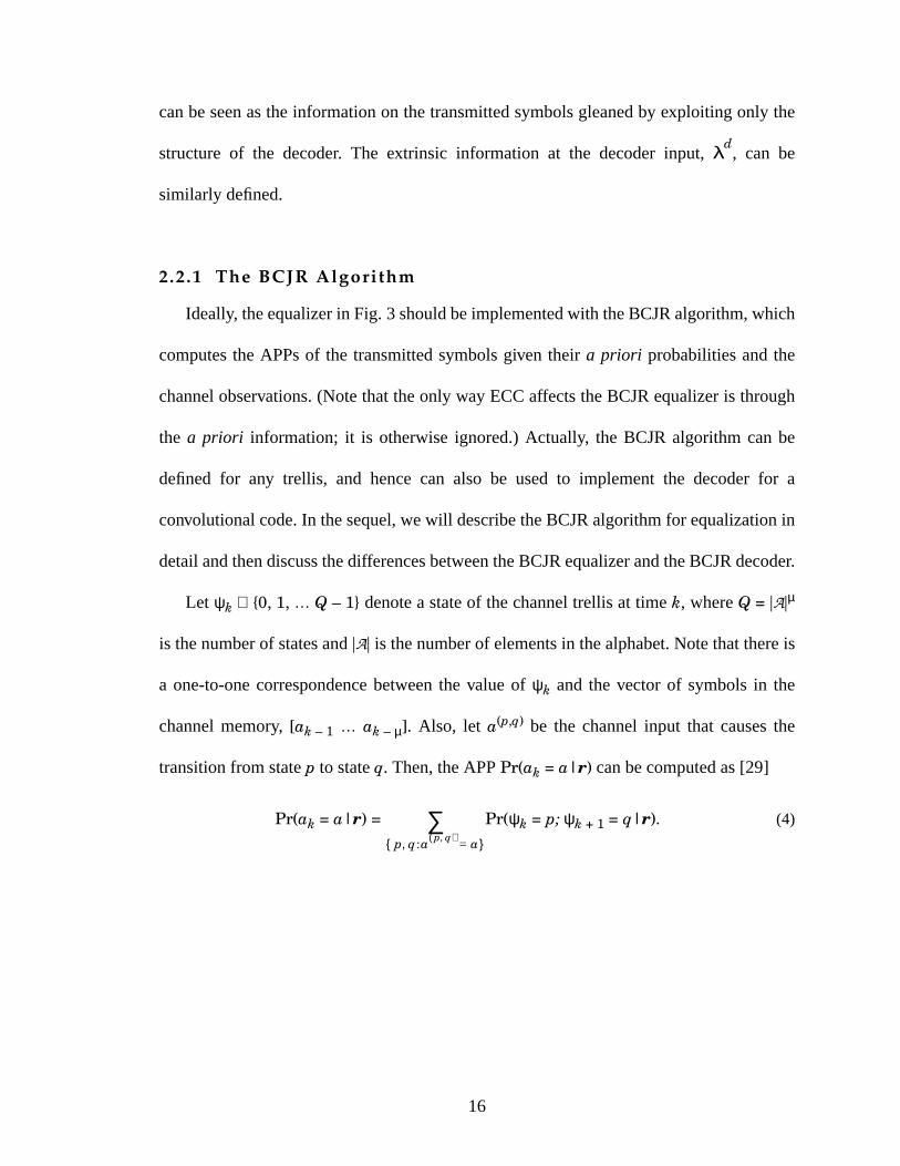
2.2.1 The BCJR Algorithm

Ideally, the equalizer in Fig. 3 should be implemented with the BCJR algorithm, which

computes the APPs of the transmitted symbols given their a priori probabilities and the

channel observations. (Note that the only way ECC affects the BCJR equalizer is through

the a priori information; it is otherwise ignored.) Actually, the BCJR algorithm can be

defined for any trellis, and hence can also be used to implement the decoder for a

convolutional code. In the sequel, we will describe the BCJR algorithm for equalization in

detail and then discuss the differences between the BCJR equalizer and the BCJR decoder.

Let ψk ∈ {0, 1, … Q – 1} denote a state of the channel trellis at time k, where Q = |A|µ

is the number of states and |A| is the number of elements in the alphabet. Note that there is

a one-to-one correspondence between the value of ψk and the vector of symbols in the

channel memory, [ak – 1 … ak – µ]. Also, let a(p,q) be the channel input that causes the

transition from state p to state q. Then, the APP Pr(ak = a|r) can be computed as [29]

Pr(ak = a|r) = Pr(ψk = p; ψk + 1 = q|r). (4)

p q:a p q,( ), a={ }∑

17

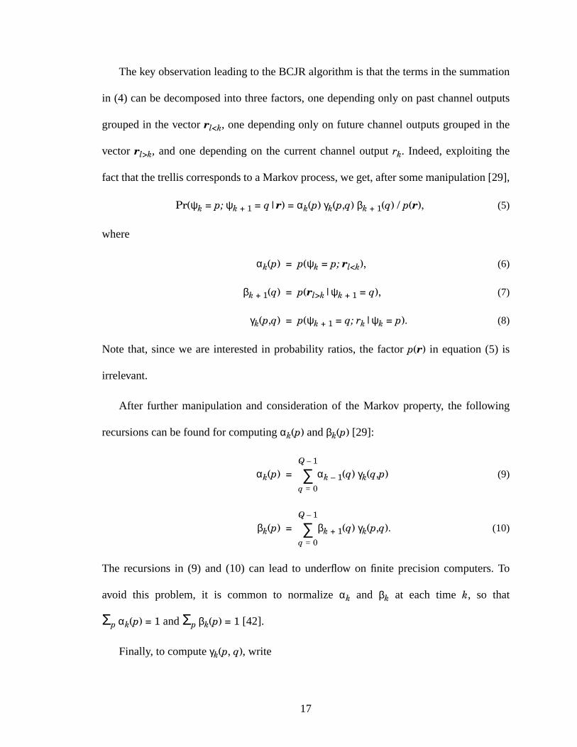
Thekey observationleadingto theBCJRalgorithmis thatthetermsin thesummation

in (4) canbedecomposedinto threefactors,onedependingonly on pastchanneloutputs

groupedin the vectorrl<k, onedependingonly on futurechanneloutputsgroupedin the

vectorrl>k, andonedependingon the currentchanneloutput rk. Indeed,exploiting the

factthatthetrellis correspondsto aMarkov process,weget,aftersomemanipulation[29],

Pr(ψk = p; ψk + 1 = q|r) = αk(p) γk(p,q) βk + 1(q) / p(r), (5)

where

αk(p) = p(ψk = p; rl<k), (6)

βk + 1(q) = p(rl>k|ψk + 1 = q), (7)

γk(p,q) = p(ψk + 1 = q; rk|ψk = p). (8)

Note that, sincewe are interestedin probability ratios,the factorp(r) in equation(5) is

irrelevant.

After further manipulationand considerationof the Markov property, the following

recursions can be found for computingαk(p) andβk(p) [29]:

αk(p) = αk – 1(q) γk(q,p) (9)

βk(p) = βk + 1(q) γk(p,q). (10)

The recursionsin (9) and (10) can lead to underflow on finite precisioncomputers.To

avoid this problem, it is common to normalize αk and βk at each time k, so that

Σp αk(p) = 1 andΣp βk(p) = 1 [42].

Finally, to computeγk(p, q), write

q 0=

Q 1–

∑

q 0=

Q 1–

∑

18

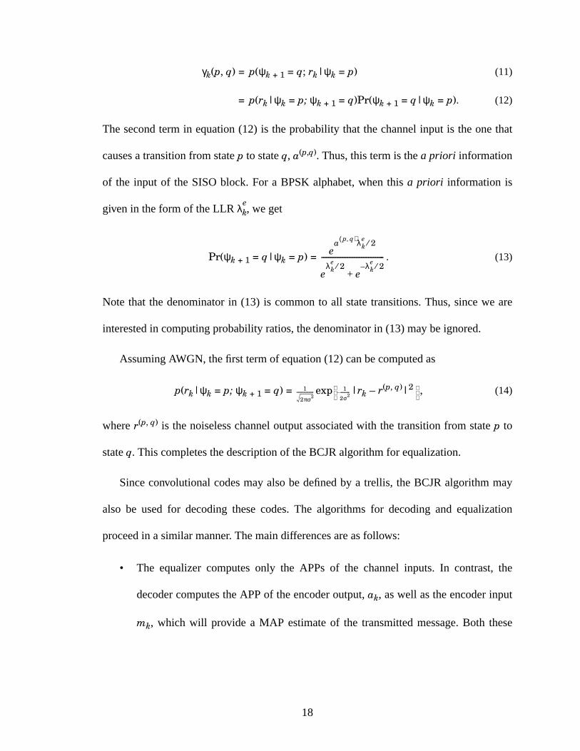
γk(p, q) = p(ψk + 1 = q; rk|ψk = p) (11)

= p(rk|ψk = p; ψk + 1 = q)Pr(ψk + 1 = q|ψk = p). (12)

The second term in equation (12) is the probability that the channel input is the one that

causes a transition from state p to state q, a(p,q). Thus, this term is the a priori information

of the input of the SISO block. For a BPSK alphabet, when this a priori information is

given in the form of the LLR λek, we get

Pr(ψk + 1 = q|ψk = p) = . (13)

Note that the denominator in (13) is common to all state transitions. Thus, since we are

interested in computing probability ratios, the denominator in (13) may be ignored.

Assuming AWGN, the first term of equation (12) can be computed as

p(rk|ψk = p; ψk + 1 = q) = exp |rk – r(p, q)|2 , (14)

where r(p, q) is the noiseless channel output associated with the transition from state p to

state q. This completes the description of the BCJR algorithm for equalization.

Since convolutional codes may also be defined by a trellis, the BCJR algorithm may

also be used for decoding these codes. The algorithms for decoding and equalization

proceed in a similar manner. The main differences are as follows:

• The equalizer computes only the APPs of the channel inputs. In contrast, the

decoder computes the APP of the encoder output, ak, as well as the encoder input

mk, which will provide a MAP estimate of the transmitted message. Both these

ea p q,( )λk

e 2⁄

eλk

e 2⁄e

λke

– 2⁄+

------------------------------------

1

2πσ2------------------ 1

2σ2----------–

1–

2σ2----------

19

APPs may be computed by considering the appropriate state transitions in the sum-

mation in (4).

• While for the equalizer each trellis stage corresponds to a single channel output,

for the decoder a trellis stage may correspond to multiple outputs. For instance, a

rate 1/2 convolutional code has two outputs for every state transition. In general,

for a rate k/n convolutional code, |rk – r(p, q)| in (14) is the distance between vec-

tors of length n.

• For turbo equalizers, such as the structure depicted in Fig. 3, the decoder does not

have access to the channel output. Therefore, (14) reduces to a constant, and the

state transition probability γk(p, q) depends only on the a priori information.

2.3 Blind Iterative Channel Estimation with the EM Algorithm

In many ML estimation problems, the difficulty in finding a solution stems from the

fact that some information about how the observed data was generated is missing. For

instance, in the blind channel estimation problem, finding the ML channel estimates

would be easy if the channel inputs were known. For ML problems that would be easily

solvable if the missing data were available, the EM algorithm is an interesting approach. It

is a low-complexity iterative algorithm that generates a sequence of estimates with non-

decreasing likelihood. Thus, with proper initialization, or if the likelihood function does

not posses local maxima, the EM algorithm will converge to the ML solution. In the

remainder of this section, we will describe the EM algorithm for blind channel estimation,

as first proposed in [22].

20

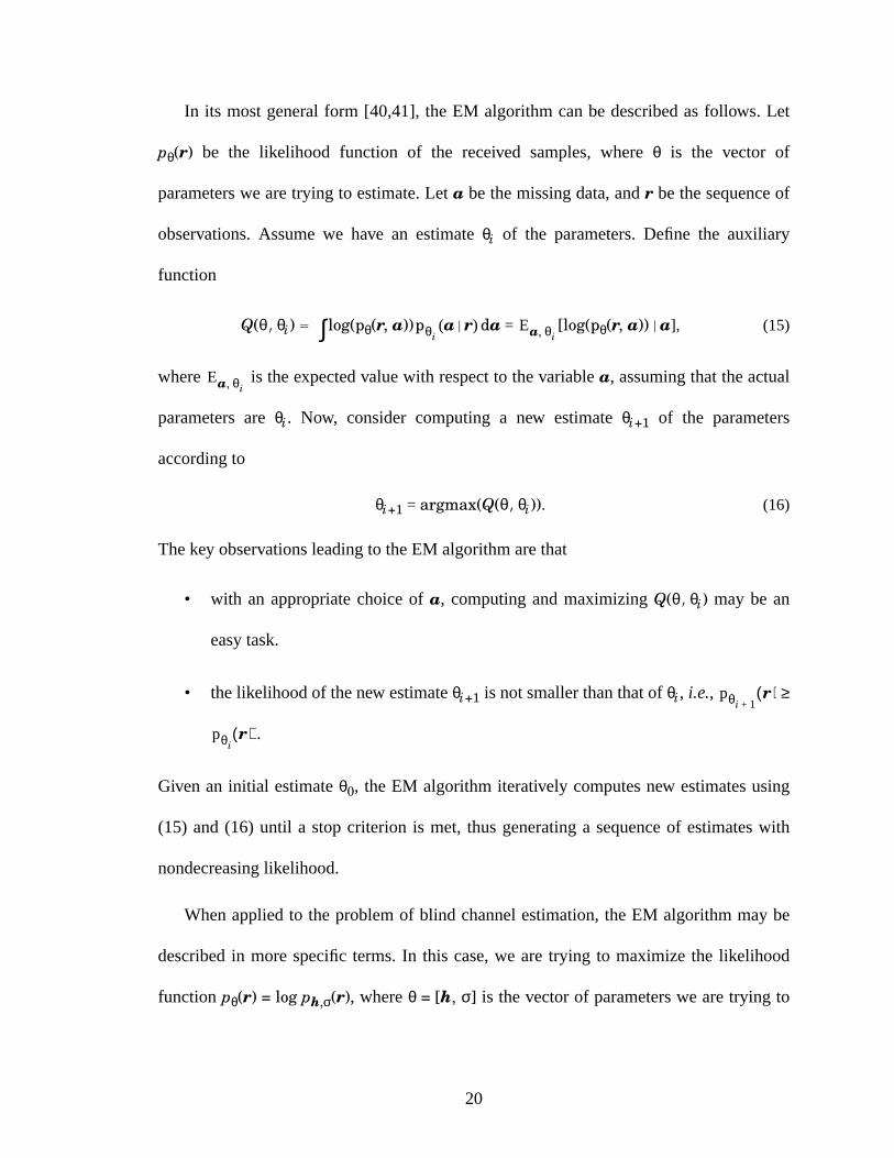
In its most general form [40,41], the EM algorithm can be described as follows. Let

pθ(r) be the likelihood function of the received samples, where θ is the vector of

parameters we are trying to estimate. Let a be the missing data, and r be the sequence of

observations. Assume we have an estimate θi of the parameters. Define the auxiliary

function

Q(θ,θi) = log(pθ(r, a)) (a|r) da = [log(pθ(r, a))|a], (15)

where is the expected value with respect to the variable a, assuming that the actual

parameters are θi. Now, consider computing a new estimate θi+1 of the parameters

according to

θi+1 = argmax(Q(θ,θi)). (16)

The key observations leading to the EM algorithm are that

• with an appropriate choice of a, computing and maximizing Q(θ,θi) may be an

easy task.

• the likelihood of the new estimate θi+1 is not smaller than that of θi, i.e., ≥

.

Given an initial estimate θ0, the EM algorithm iteratively computes new estimates using

(15) and (16) until a stop criterion is met, thus generating a sequence of estimates with

nondecreasing likelihood.

When applied to the problem of blind channel estimation, the EM algorithm may be

described in more specific terms. In this case, we are trying to maximize the likelihood

function pθ(r) = log ph,σ(r), where θ = [h, σ] is the vector of parameters we are trying to

∫ pθiEa θi,

Ea θi,

pθi 1+r( )

pθir( )

21

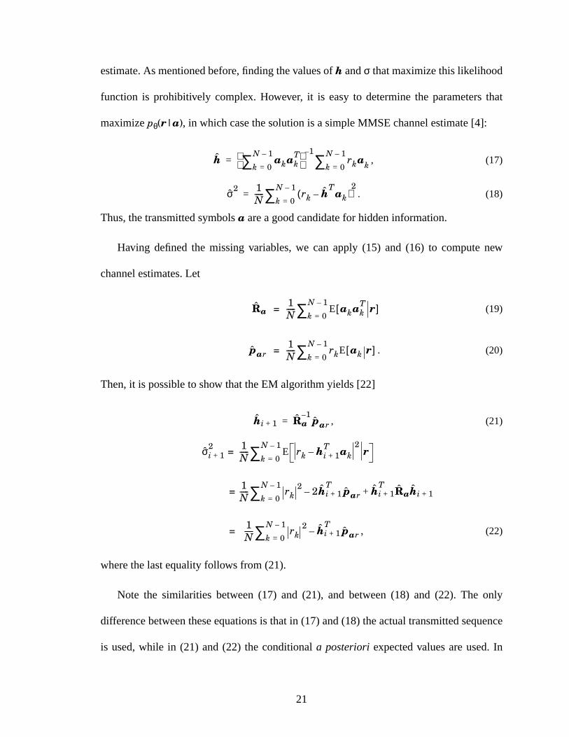
estimate. As mentioned before, finding the values of h and σ that maximize this likelihood

function is prohibitively complex. However, it is easy to determine the parameters that

maximize pθ(r|a), in which case the solution is a simple MMSE channel estimate [4]:

, (17)

. (18)

Thus, the transmitted symbols a are a good candidate for hidden information.

Having defined the missing variables, we can apply (15) and (16) to compute new

channel estimates. Let

= (19)

= . (20)

Then, it is possible to show that the EM algorithm yields [22]

, (21)

=

=

= , (22)

where the last equality follows from (21).

Note the similarities between (17) and (21), and between (18) and (22). The only

difference between these equations is that in (17) and (18) the actual transmitted sequence

is used, while in (21) and (22) the conditional a posteriori expected values are used. In

h akakT

k 0=

N 1–∑ 1–

rkakk 0=

N 1–∑=

σ2 1N----- rk h

Ta– k( )

2

k 0=

N 1–∑=

Ra1N----- E akak

T r[ ]k 0=

N 1–∑

par1N----- rkE ak r[ ]

k 0=

N 1–∑

hi 1+ Ra1–

par=

σi 1+2 1

N----- E rk hi 1+

T ak–2

rk 0=

N 1–∑

1N----- rk

2 2hi 1+T

par– hi 1+T

Rahi 1++k 0=

N 1–∑

1N----- rk

2 hi 1+T

par–k 0=

N 1–∑

22

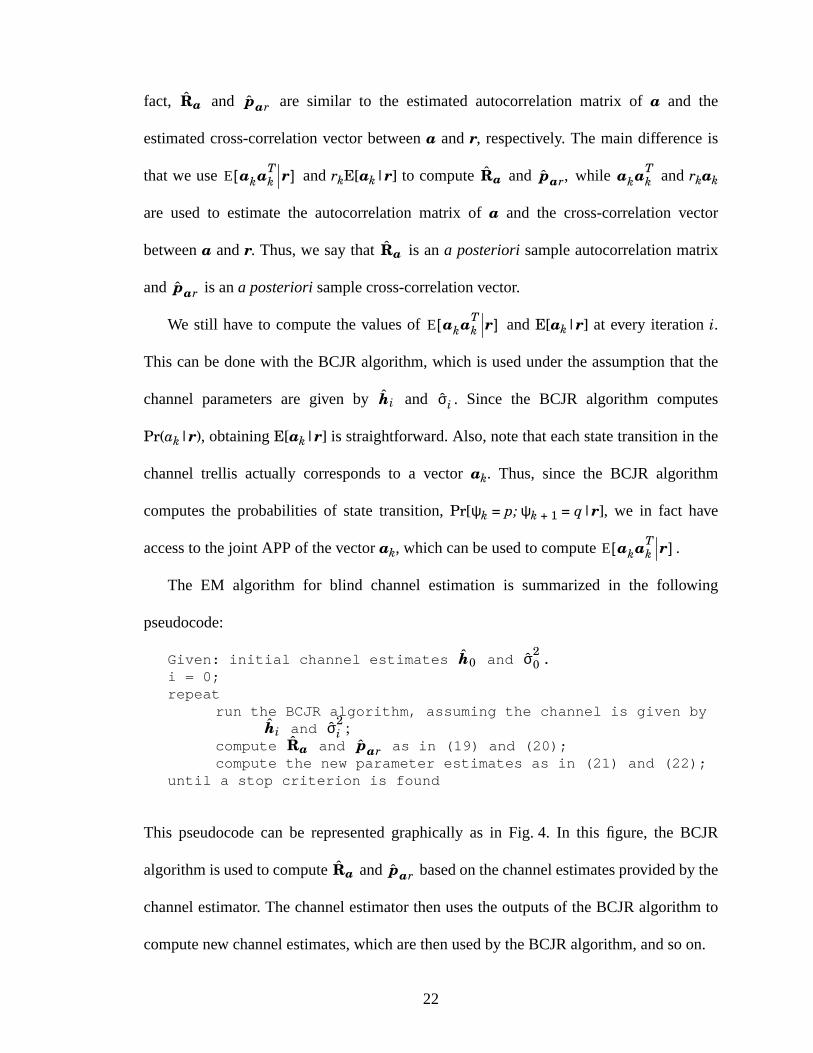
fact, and are similar to the estimated autocorrelation matrix of a and the

estimated cross-correlation vector between a and r, respectively. The main difference is

that we use and rkE[ak|r] to compute and , while and rkak

are used to estimate the autocorrelation matrix of a and the cross-correlation vector

between a and r. Thus, we say that is an a posteriori sample autocorrelation matrix

and is an a posteriori sample cross-correlation vector.

We still have to compute the values of and E[ak|r] at every iteration i.

This can be done with the BCJR algorithm, which is used under the assumption that the

channel parameters are given by and . Since the BCJR algorithm computes

Pr(ak|r), obtaining E[ak|r] is straightforward. Also, note that each state transition in the

channel trellis actually corresponds to a vector ak. Thus, since the BCJR algorithm

computes the probabilities of state transition, Pr[ψk = p; ψk + 1 = q|r], we in fact have

access to the joint APP of the vector ak, which can be used to compute .

The EM algorithm for blind channel estimation is summarized in the following

pseudocode:

Given: initial channel estimates and .i = 0;repeat

run the BCJR algorithm, assuming the channel is given by and ;

compute and as in (19) and (20);compute the new parameter estimates as in (21) and (22);

until a stop criterion is found

This pseudocode can be represented graphically as in Fig. 4. In this figure, the BCJR

algorithm is used to compute and based on the channel estimates provided by the

channel estimator. The channel estimator then uses the outputs of the BCJR algorithm to

compute new channel estimates, which are then used by the BCJR algorithm, and so on.

Ra par

E akakT r[ ] Ra par akak

T

Ra

par

E akakT r[ ]

hi σi

E akakT r[ ]

h0 σ02

hi σi2

Ra par

Ra par

23

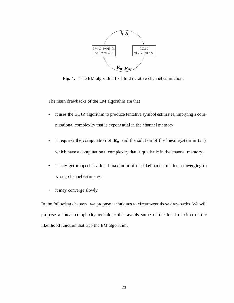
The main drawbacks of the EM algorithm are that

• it uses the BCJR algorithm to produce tentative symbol estimates, implying a com-

putational complexity that is exponential in the channel memory;

• it requires the computation of and the solution of the linear system in (21),

which have a computational complexity that is quadratic in the channel memory;

• it may get trapped in a local maximum of the likelihood function, converging to

wrong channel estimates;

• it may converge slowly.

In the following chapters, we propose techniques to circumvent these drawbacks. We will

propose a linear complexity technique that avoids some of the local maxima of the

likelihood function that trap the EM algorithm.

Fig. 4. The EM algorithm for blind iterative channel estimation.

h σ,

BCJRALGORITHM

EM CHANNELESTIMATOR

Ra par,

Ra

24

CHAPTER 3

A Simplified EM Algorithm

As mentioned in Chapter 2, some of the complexity issues associated with the EM

algorithm stem from the need to compute and invert the a posteriori sample

autocorrelation matrix defined in (19). In this chapter, we derive the simplified EM

algorithm (SEM), an alternative iterative channel estimator that ignores and yet does

not significantly degrade the performance relative to the EM algorithm. For notational

convenience, in what follows we assume that the transmitted symbols belong to a BPSK

constellation. Generalization to other constellations is straightforward.

3.1 Derivation of the SEM Algorithm

Consider the channel model in equation (1), repeated here for convenience

rk = hTak + nk. (23)

Assuming that the transmitted symbols are uncorrelated, we have

hn = E[rkak–n] (24)

= E[rkPr(ak–n = + 1|rk)] – E[ rkPr(ak–n = – 1 |rk)] (25)

= E[rkPr(ak–n = + 1|r) – rkPr(ak–n = – 1 |r)] (26)

= E[rk E[ak–n|r]]. (27)

Ra

Ra

25

This equationleadsto a simplechannelestimator. Unfortunately, the channelestimator

hasno accessto E[ak|r], which requiresexact channelknowledge.However, basedon

theiterativeparadigmof Fig. 1, at thei-th iterationthechannelestimatordoeshaveaccess

to = = tanh(Lk ⁄ 2). Using this value in (27), and also replacing

ensembleaveragewith time average,the channelestimateat the i+1-st iterationis given

by:

= rktanh . (28)

Thus,(28) providesa methodfor estimatingthechannelgiven thesoft symbolestimates

Lk, and can be used in the samecontext as the channelestimationstep of the EM

algorithm.Clearly, its implementationhasa per-symbolcomplexity that is linear in the

length of the channel if the LLRs are given.

For estimatingthenoisevarianceσ2 at thei-th iteration,we proposeusingthechannel

estimatesin (28) andthebit estimatesobtainedfrom Lk to estimatethenoisecomponent

of thereceivedsignal,which arethenusedto estimatethenoisevariance.In otherwords,

letting = [ , … ]T, where = sign(Lk), we estimate the noise variance as

= , (29)

where = [ , … ]T. This estimatediffersfrom theEM estimatein (22),

but in our simulationswe notedthatusing insteadof E[ak|r] for estimatingthenoise

varianceimprovedconvergencespeed.Furtherjustificationfor theuseof harddecisionsin

(29) will be given in the next section.

The resulting algorithm is described by the following pseudocode:

aki( )

E ak r hi σi,;[ ]

hn i 1+,1N-----

k 0=

N 1–∑Lk n–

2--------------

ak ak ak µ– ak

σi 1+2 1

N----- rk ak

Thi 1+–2

k 0=

N 1–

∑

hi 1+ h0 i 1+, hµ i 1+,

ak

26

initialize channel estimates and ;i = 0;repeat

use channel estimates to compute symbol estimates Lk, fork = 0, … N-1;

update channel estimates using (28) and (29);i = i + 1;

until a stop criterion is met

This algorithm will be referred to as simplified EM (SEM). Indeed, using the notation

from chapter 2, comparing (20) and (28) we see that . Therefore, (28) can be

seen as a simplification of the EM algorithm wherein is replaced by I. It is important

to point out that, from (19), ≈ I is a reasonable approximation. In fact, is

the MMSE estimate of given the current channel estimate. Thus, these two values

are expected to be approximately the same, so that is approximately a time-average

estimate of the autocorrelation matrix of the transmitted symbols. Since we assumed that

the channel input is white, based on the law of large numbers should be close to the

identity for large enough N.

An important implication of ignoring the matrix is that the channel estimator

requires only the soft symbol estimates Lk. Thus, we may represent the simplified channel

estimator as in Fig. 5, where the symbol estimator is not restricted to be the BCJR

h0 σ02

hi 1+ par=

Ra

Ra E akakT r[ ]

akakT

Ra

Ra

Ra

Fig. 5. Blind iterative channel estimation with the SEM algorithm.

h σ,

SYMBOLESTIMATOR

CHANNELESTIMATOR

Lk

27

equalizer. In fact, any equalizerthat producessoft symbolestimatescanbe used,which

allows for a low-complexity implementationof the blind iterative channelestimator.

Contrastthis figurewith Fig. 4, which representstheEM algorithm.In theEM algorithm,

theequalizeris restrictedto be theBCJRalgorithm,andit alsomustprovide a matrix to

the channel estimator.

3.2 Analysis of the Scalar Channel Estimator

In thissection,weprovideadetailedanalysisof theSEMalgorithmappliedto ascalar

channel.Althougha detailedanalysisof theSEM algorithmfor a generalchannelwould

be of moreinterest,this analysisis difficult. Furthermore,scalarchannelsestimatorsare

important,beingusedin systemsthat aresubjectto flat fading [43] and in systemsthat

employ multicarriermodulation[44]. In performingthis analysis,we will alsocompare

theperformanceof systemsusingsoft andharddecisions.In particular, wewill justify the

use of hard decisions for estimating the noise variance in (29).

Considerthe transmissionof a sequenceof uncorrelatedbits ak ∈ {–1,+1} througha

scalarchannelwith gain A, theoutputof which is corruptedby anAWGN componentnk

with varianceσ2. The received signal can be written as

rk = A ak + nk. (30)

Given initial estimates and , the channelgain and noise variancecan be

estimated with an iterative algorithm. Possible estimators can be expressed as

= , (31)

A0 σ0

Ai 1+1N----- rk

k 0=

N 1–

∑ decA12--- Lirk

28

= , (32)

where i is the iteration number, = 2 / is the estimated channel reliability and

where decA(⋅) and decσ(⋅) are decision functions, given by either tanh(⋅) or sign(⋅). We

will consider four different estimators, denoted SS, SH, HS and HH, where the first S or H

indicates whether soft or hard information, respectively, is used for gain estimation, and

the second S or H indicates whether soft or hard information, respectively, is used for

estimating noise variance. Note that the SH estimator corresponds to the SEM algorithm

applied to a scalar channel. The EM algorithm, on the other hand, cannot be expressed in

this framework. Its channel gain estimator can be expressed as in (31), with decA(⋅) =

tanhA (⋅). Its noise variance estimator, however, is given by

=

= . (33)

Now suppose the number of observations tends to infinity. In this case, we may use the

law of large numbers in (31), and (32). Thus, in this asymptotic case, the channel HH, SH,

SS and HS estimators may be written as

= E . (34)

= E . (35)

σi 1+2 1

N----- rk Ai 1+ decσ

12--- Lirk

–2

k 0=

N 1–

∑

Li Ai σi2

σi 1+2 1

N----- rk

2 Ai 1+2

2rk Ai 1+ tanh 12--- Lirk

–+k 0=

N 1–

∑

1N----- rk

2 Ai 1+–k 0=

N 1–

∑

Ai 1+ rkdecA12--- Lirk

σi 1+2 rk Ai 1+ decσ

12--- Lirk

–2

29

Equation (34) also describes the gain estimator of the EM algorithm. The noise variance

estimator for the EM algorithm is obtained by applying the law of large numbers in (33),

yielding

= E – (36)

= A2 + σ2 – . (37)

For the HH estimator, it is shown in Appendix A that (34) and (35) may be written in

closed form as

= A (1 – 2 Q ) + , (38)

and

= A2 + σ2 – , (39)

with ≥ ≥ A. Therefore, for the HH estimator neither nor depend

on the iteration number i. Unfortunately, if soft information is used, equation (34) cannot

be computed in closed form, so we must resort to numerical integration.

From (34), (35) and (37), we see that, as N tends to infinity, , and consequently

, is a function of just . The fact that both and depend on a single

parameter allows for a graphical study of the iterative process. This analysis is clearer if

we consider the ratio αi = / L instead of , where αi is the relative estimated channel

reliability, defined as the ratio between the estimated channel reliability at the i-th iteration

and the actual channel reliability L = 2A ⁄ σ2. For the graphical analysis, we view one

iteration of the SEM algorithm as a function whose input is αi and whose output is αi+1.

σi 1+2 rk

2[ ] Ai 1+2

Ai 1+2

Ai 1+Aσ----

2π---σ A2

2σ2----------–

exp

σ2i 1+ Ai 1+

2

A2 σ2+ A Ai 1+ σ2

i 1+

Ai 1+

σi 1+2 Li Ai 1+ σi 1+

2

Li Li

30

This function is plotted in a graph, along with the line αi+1 = αi. Since the algorithm

converges when αi = αi+1, the fixed points of the SEM algorithm are given by the

intersection of the two curves.

In Fig. 6 we plot αi+1 versus αi for the five estimators, assuming A = and an SNR

= A2 ⁄ σ2 = 2 dB. We also plot the line αi+1 = αi, which allows for the graphical

determination of the behavior of the algorithms as follows. Initially, at the zero-th

iteration, a value α0 is given. The estimator then produces a value of α1, which can be

determined graphically as shown by the vertical arrow in Fig. 6 for the EM algorithm and

α0 = 2.2. The value of αi for the next iteration can now be found by the vertical arrow in

Fig. 6, which connects the point (α0, α1) to the point (α1, α1). Now the value of α2 can be

determined by a vertical line, not shown in Fig. 6, that connects the point (α1, α1) to the

HH

SEM

SS

HS

αi+1 = αi

EM

Fig. 6. Estimated relative channel reliability αi as a function of its value in theprevious iteration, αi–1.

αi

α i+

1

0 0.5 1 1.5 2 2.5

0

0.5

1

1.5

2

2.5

2

31

EM curve.Theprocessthenrepeats.It is clearthattheiterationsstopwhenthecurve for a

givenalgorithmintersectstheline αi+1 = αi. Thevaluesfor which thishappens,α∗, arethe

fixed point of the algorithms and are marked with ‘×’ in Fig. 6.

Someinterestingobservationscanbemadefrom Fig. 6. Consider, for instance,theHH

estimator. For this estimator, we seein Fig. 6 thatthevalueof αi+1 doesnot dependon αi.

Thus, following the iterative procedure,we seethat the HH algorithm converges in a

singleiteration,aswasexpectedfrom theanalysisin (38) and(39). We canalsoseethat

theEM andtheSEMalgorithmsgenerateamonotonesequenceαi. In otherwords,if these

algorithmsareinitialized with anα0 larger(smaller)thantheir fixedpoint α∗, thenαi will

monotonicallydecrease(increase)until they converge.On the otherhand,the αi for the

HS and SS algorithms eventually becomegreater than α∗. After that happens,they

alternate between values that are greater than and smaller thanα∗.

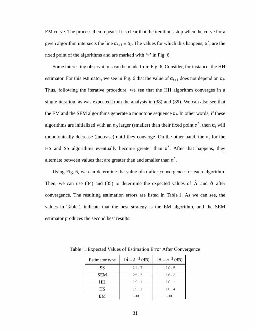
Using Fig. 6, we candeterminethe valueof α after convergencefor eachalgorithm.

Then, we can use (34) and (35) to determinethe expectedvaluesof and after

convergence.The resultingestimationerrorsare listed in Table1. As we can see,the

values in Table1 indicate that the best strategy is the EM algorithm, and the SEM

estimator produces the second best results.

A σ

Table 1:Expected Values of Estimation Error After Convergence

Estimator type |Â – A|2 (dB) | – σ|2 (dB)

SS -21.7 -10.5

SEM -25.3 -16.2

HH -19.1 -16.1

HS -19.1 -10.4

EM –∞ –∞

σ

32

Even though the EM algorithm is expected to produce exact estimates, its convergence

can be very slow. This can be seen in Fig. 7, where we plot the expected trajectories of the

EM and the SEM algorithms, assuming that both algorithms are initialized using the HH

estimates. The HH estimates are a good candidate for initialization: they have reasonable

performance and converge in one iteration. As we can see in Fig. 7, the SEM estimator is

expected to converge in roughly 2 iterations, while the EM estimator is expected to

converge in roughly 7 iterations.

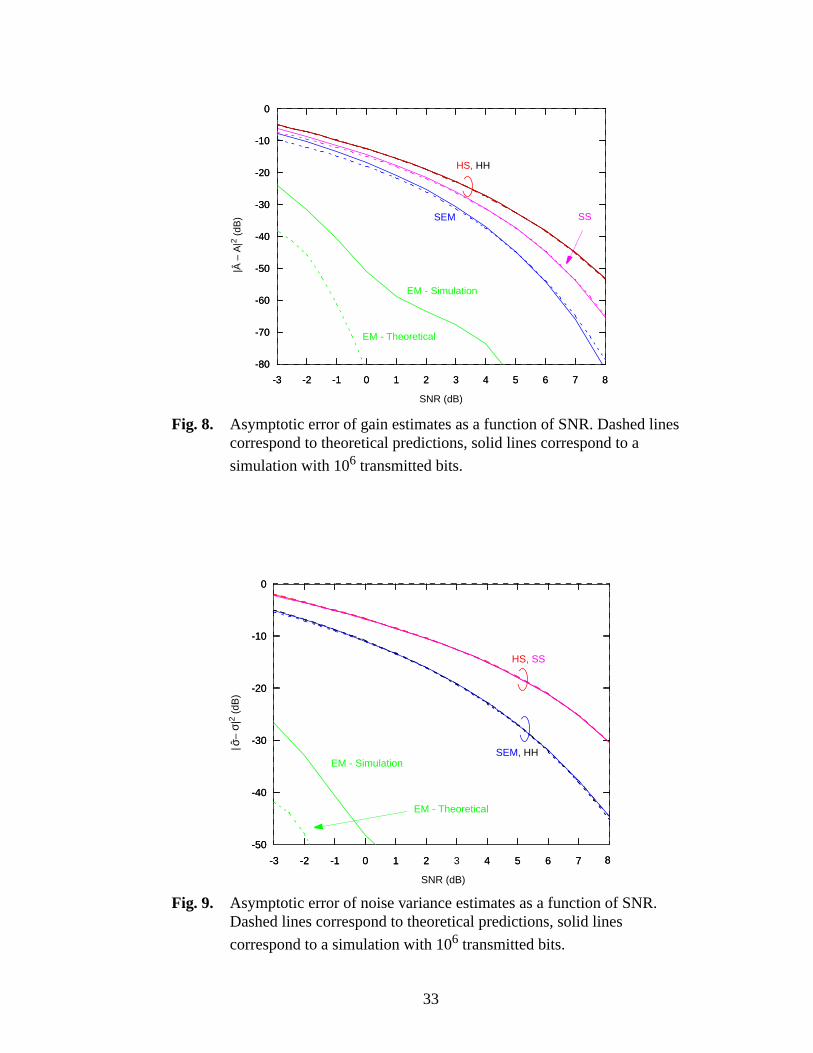
The performance of the estimators can be computed using the method described above

for other values of SNR, yielding the plots of the estimation errors for and versus

SNR shown in the dashed lines in Fig. 8 and Fig. 9, respectively. Again, we see that the

EM algorithm gives the best overall performance, followed by the SEM estimator. For

comparison, we also show simulation results in Fig. 8 and Fig. 9. These correspond to the

EM

Fig. 7. Tracking the trajectories of the EM and the SEM estimators for a scalarchannel.

αi

α i+

1

0.9 1 1.1 1.2 1.3 1.4 1.5

0.9

1

1.1

1.2

1.3

1.4

1.5

HH

SEM

α i+1 =

α i

A σ2

33

Fig. 8. Asymptotic error of gain estimates as a function of SNR. Dashed linescorrespond to theoretical predictions, solid lines correspond to a

simulation with 106 transmitted bits.

|–

A|2

(dB

)

HS, HH

SSSEM

SNR (dB)

-3 -2 -1 0 1 2 3 4 5 6 7 8

-80

-70

-60

-50

-40

-30

-20

-10

0

-3 -2 -1 0 1 2 3 4 5 6 7 8

-80

-70

-60

-50

-40

-30

-20

-10

0

EM - Simulation

EM - Theoretical

3

SEM, HH

HS, SS

Fig. 9. Asymptotic error of noise variance estimates as a function of SNR.Dashed lines correspond to theoretical predictions, solid lines

correspond to a simulation with 106 transmitted bits.

| –

σ|2

(dB

)σ

SNR (dB)

-3 -2 -1 0 1 2 4 5 6 7 8

-50

-40

-30

-20

-10

0

-3 -2 -1 0 1 2 4 5 6 7 8

-50

-40

-30

-20

-10

0

EM - Simulation

EM - Theoretical

34

solid lines, and were obtained using 106 transmitted bits, and the channel estimators were

run until | – | < 10–5 or the number of iterations exceeded 20. As we can see, the

theoretical curves predict the performance of the estimators very closely, except for the

EM algorithm. An explanation for the difference between the theoretical and simulation

curves for the EM algorithm could not be found.

3.3 The Impact of the Estimated Noise Variance

It is interesting to note that while substituting the actual values of h or a for their

estimates will always improve the performance of the iterative algorithm, the same is not

true for σ. Indeed, substituting σ for will often result in performance degradation.

Intuitively, one can think of as playing two roles: in addition to measuring σ, it also acts

as a measure of reliability in the channel estimate . Consider a decomposition of the

channel output:

rk = ak + (h – )Tak + nk. (40)

The term (h – )Tak represents the contribution to rk from the estimation error. By using

to model the channel in the BCJR algorithm, we are in effect lumping the estimation

error with the noise. Combining the two results in an effective noise sequence with

variance larger than σ2. It is thus appropriate that should exceed σ whenever differs

from h. Alternatively, it stands to reason that an unreliable channel estimate should

translate to an unreliable (i.e., with small magnitude) symbol estimate, regardless of how

well ak matches rk. Using a large value of in the BCJR equalizer ensures that its

output will have a small magnitude. Fortunately, the noise variance estimate produced by

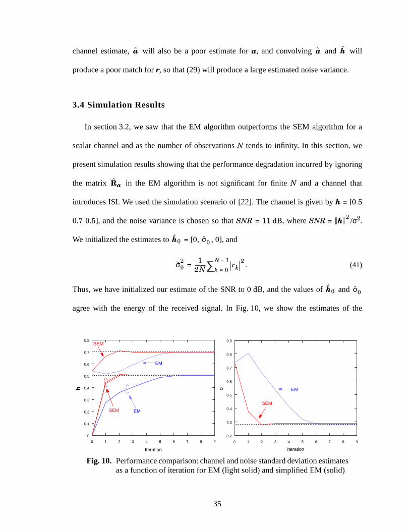
(29) measures the energy of both the second and the third term in (40). If is a poor

Li Li 1–

σ

σ

h

hT

h

h

h

σ h

hT

σ

h

35

channelestimate, will also be a poor estimatefor a, and convolving and will

produce a poor match forr, so that (29) will produce a large estimated noise variance.

3.4 Simulation Results

In section3.2, we saw that the EM algorithmoutperformsthe SEM algorithmfor a

scalarchannelandasthe numberof observationsN tendsto infinity. In this section,we

presentsimulationresultsshowing that theperformancedegradationincurredby ignoring

the matrix in the EM algorithm is not significant for finite N and a channelthat

introducesISI. We usedthesimulationscenarioof [22]. Thechannelis givenby h = [0.5

0.7 0.5], andthe noisevarianceis chosenso that SNR = 11 dB, whereSNR = /σ2.

We initialized the estimates to = [0, , 0], and

= . (41)

Thus,we have initialized our estimateof theSNRto 0 dB, andthevaluesof and

agreewith the energy of the received signal. In Fig. 10, we show the estimatesof the

a a h

Ra

h 2

h0 σ0

σ02 1

2N--------- rk

2k 0=

N 1–∑

h0 σ0

Fig. 10. Performancecomparison:channelandnoisestandarddeviationestimatesas a function of iteration for EM (light solid) and simplified EM (solid)

0 1 2 3 4 5 6 7 8 9

0

0.1

0.2

0.3

0.4

0.5

0.6

0.7

0.8

Iteration

h

0 1 2 3 4 5 6 7 8 9

0.2

0.3

0.4

0.5

0.6

0.7

0.8

0.9

Iteration

σ

EM

EM

EM

SEM

SEM

SEM

36

channel coefficients and the noise standard deviation as a function of iteration for the EM

and the SEM algorithms, averaged over 100 independent blocks of 256 BPSK symbols.

As expected, the SEM algorithm yields a larger estimation error than the EM algorithm,

though the performance loss is not significant. As in the scalar channel case, the SEM

algorithm converges faster than EM in this experiment.

In this chapter, we only simulated the performance of the SEM algorithm for one ISI

channel. In Chapter 4, we introduce a modification to the SEM algorithm that greatly

improves its convergence. More simulations will be conducted then.

3.5 Summary

In this section, we proposed the SEM algorithm, an iterative blind channel estimator

that is less complex than the EM algorithm in two ways: it does not require the

computation and inversion of the autocorrelation matrix, and it is not intrinsically tied to

the BCJR equalizer. We presented an asymptotic analysis of different estimators,

including the SEM and EM algorithms, for a scalar channel and as the number of

observations tends to infinity. We showed that the EM algorithm provides the best

estimates in this case, followed by the SEM algorithm. We also showed that for a scalar

channel the SEM algorithm is expected to converge faster than the EM algorithm. For a

channel that introduces ISI, simulation results indicate that the performance loss of the

SEM is not significant when compared to the EM algorithm, and that the SEM estimates

converge faster than the EM estimates.

37

CHAPTER 4

The Extended-Window Algorithm (EW)

As we discussed in section 2.3, the EM algorithm generates a sequence of estimates

with nondecreasing likelihood. Thus, it is prone to misconvergence, defined in the present

context as the convergence to a nonglobal local maximum of the likelihood function. The

traditional approach to this problem is either to completely ignore misconvergence or to

assume the availability of a good initialization. For instance, the simulation in the previous

section involved some cheating: the channel estimates were initialized to an impulse at the

center tap, which happens to match the main tap of the channel. However, there is no

reason for using such initialization other than the fact that we know that the center tap of

the actual channel is dominant, a knowledge that obviously would not be available in a

real-world blind application. In this chapter, we show that the estimates after

misconvergence may have a structure that allows some local maxima to be escaped.

4.1 A Study of Misconvergence

To study an example of misconvergence, consider using the SEM algorithm to identify

the maximum-phase channel h = [1 2 3 4 5]T at SNR = 24 dB, with a BPSK input

sequence. With the channel estimates being initialized to = [1 0 0 0 0]T and = 1,

after 20 iterations the SEM algorithm converged to a fixed point of

h0 σ0

38

= [2.1785 3.0727 4.1076 5.0919 0.1197]T. (42)

The algorithm thus fails. But the estimated channel is roughly a shifted version of h. A

possible explanation for this behavior is that, if the channel is not minimum phase, then it

introduces some delay δ that cannot be compensated for at the symbol estimator of Fig. 5.

Thus, the soft symbol estimate Lk produced by the symbol estimator may in fact be related

to a delayed symbol ak – δ, i.e., Lk ≈ log Pr(ak – δ = + 1|r) ⁄ Pr(ak – δ = –1| r). Therefore,

when using equation (28) to estimate hn, we may be estimating hn + δ instead. In this

example, the delay is 1. Apart from this delay, the algorithm seems to perform well, and in

fact if it were to also compute

E rktanh , (43)

it would also be able to accurately estimate h0. Hence, to estimate all the channel

coefficients in this example, we must compute equation (28) for more values than

originally suggested by the EM algorithm.

For a general channel, we have observed that, after convergence, the sign of the LLR

produced by the BCJR algorithm is related to the actual symbol ak by sign(Lk) ≈ ak – δ, for

some integer delay δ satisfying |δ| ≤ µ. Even though a proof of this bound for the delay

could not be obtained, there is an intuitive explanation for this behavior. Let d =

argmax0 ≤ j ≤ µ|hj|. If the actual channel were known to the symbol estimator, then rk is

the channel output that has the largest impact on the decision made on ak – d. Now assume

that the channel estimator passes to the symbol estimator, and let = argmax0 ≤ j ≤ µ

| |. With this channel estimate, the symbol estimator will be such that rk is the channel

output that has the largest impact on the decision made on . If this estimate is

h

1---Lk 1+

2--------------

h d

h j

ak d–

39

reasonable,then ≈ ak – d, since they are both mostly influencedby rk. In other

words, after convergence,sign(Lk) ≈ . Now let δ = d – . Since d, ∈

{0, … µ}, we indeed have |δ| ≤ µ.

To illustrate the effectsof the delay in channelestimation,considerfor instancethe

channelh = [1 ε ε ε ε]T for somesmallε, andassumethatthechannelestimatorpasses

= [0 0 0 0 1]T anda given 2 to thesymbolestimator. With thesevalues,theoutputof the

symbolestimatorwould essentiallybeLk = 2rk + 4/ 2. But we know that,for thechannel

h, sign(rk) ≈ ak, andhencesign(Lk) ≈ ak + 4. Thus,if wecompute(28) for n = –4, … 0, as

originally suggested, we will never get a chance to compute, for instance,

1 = rkak–1 ≈ rktanh(Lk – 5 ⁄ 2). (44)

Likewise,if h = [ε ε ε ε 1]T, andthechannelestimatorpasses = [1 0 0 0 0]T anda given

2 to the symbolestimator, thenwe would have Lk = 2rk/ 2, so that sign(Lk) ≈ ak – 4.

Thus,if wecompute(28) for thegivenwindow n = –4, … 0, wewouldnevergetachance

to estimate 1. For that, we would have to useLk + 3. Even thoughtheseare extreme

examples, they illustrate well the effects of the delay in the iterative process.

4.2 The EW Channel Estimator

In light of the discussionabove, it is clear that if we are to correctly estimatethe

channel,we cannotrestrictthecomputationof (28) to thewindow n = – µ, … 0. Thus,we

proposean extended window EM (EW) algorithm.To determinehow muchthe window

must be extended,we again considerthe extreme cases.When sign(Lk) ≈ ak – µ, to

ak d–

ak d d–( )– d d

h

σ

σ

h 1N-----

k 1=

N

∑ 1N-----

k 1=

N

∑

h

σ σ

h

40

estimate h0 and hµ we need to compute (28) for n = – µ and n = 0, respectively. Likewise,

when sign(Lk) ≈ ak + µ, to estimate h0 and hµ we need to compute (28) for n = µ and n =

2µ, respectively. Thus, we propose to compute an auxiliary vector g as

gn = rktanh , for n = – µ, …, 2µ. (45)

Note that only µ+1 adjacent elements of g are expected to be non-zero. With that in mind,

we propose that the channel estimates be the µ+1 adjacent elements of g with highest

energy.

4.2.1 Delay and Noise Variance Estimator

Let = [g�– δ, … g– δ + µ]T be the portion of g with largest energy. Note that after

convergence we expect that = h, i.e., g– δ = h0. But comparing (25) and (45), we note

that this is equivalent to saying that

ak ≈ tanh . (46)

In other words, by choosing to be the current channel estimate we are inherently

assuming that the estimated sequence is a delayed version of the transmitted one, where

the delay is δ. This delay should be taken into account in the estimation of the noise

variance. With that in mind, we propose to estimate σ2 using a modified version of (29),

namely

= . (47)

The EW algorithm is summarized in the following pseudocode:

1N----- ---

k 1=

N∑Lk n–

2--------------

h

h

h

Lk δ+

2--------------

h

σi 1+2 1

N----- rk ak δ–

T hi 1+–2

k 1=

N

∑

41

initialize channel estimates and .i = 0.repeat

use current channel estimates to compute symbol estimatesLk, for k = 0, … N-1.

Compute gn, n = –µ, … 2µ, as in (45).Let = [g–d, … g–d + µ]

T be the µ+1 consecutive entriesof g with highest energy.

Update the noise variance estimate according to (47).i = i + 1.

until a stop criterion is met

4.3 Simulation Results

In this section, we present some simulation results comparing the performance of the

EW algorithm to the EM algorithm and to trained channel estimation algorithms. In all the

simulations, we have used a BCJR equalizer with the EW algorithm, to allow for a fair

comparison with the EM algorithm. The results presented in this section all correct for the

aforementioned delays in the channel estimation process. In other words, when computing

estimation error or averaging channel estimates, the estimates were shifted to best match

the actual channel. Note that this does not affect the channel estimates in the iterative

procedure.

As a first test of the extended-window algorithm, we simulated the transmission of K =

600 bits over the channel h = [–0.2287, 0.3964, 0.7623, 0.3964, –0.2287] T from [26],

whose frequency response is shown in Fig. 11. We have used SNR = /σ2 = 9 dB. To

stress the fact that the proposed algorithm is not sensitive to initial conditions, we

initialized randomly using = u , where u ~ N(0, I) and =

⁄ 2N. (This implies an initial estimated SNR of 0 dB, with values consistent

with the received energy.) In Fig. 12, we show the convergence behavior of the SEM

h0 σ02

hi

h 2

h h 0( ) σ 0( ) u⁄ σ 0( )2

rk2

k 0=

N 1–∑

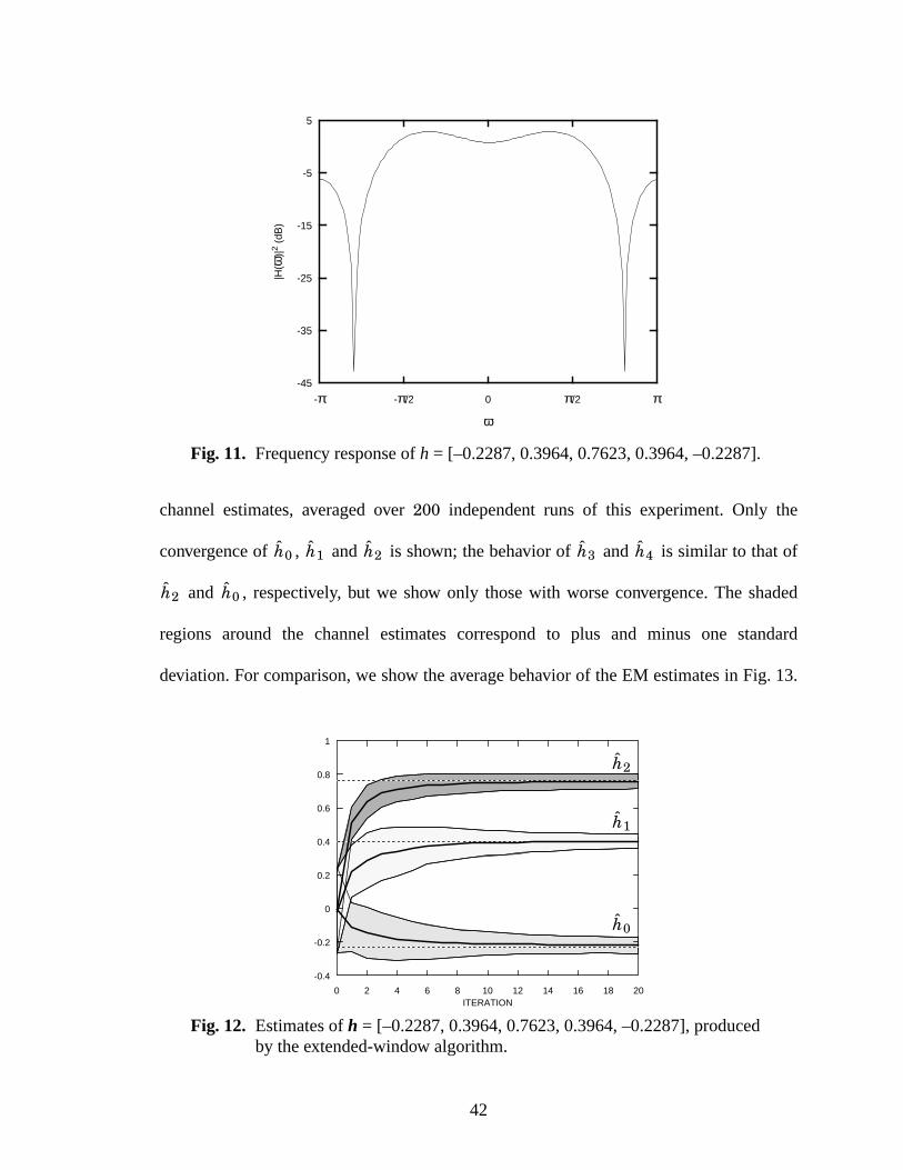
42

channel estimates, averaged over 200 independent runs of this experiment. Only the

convergence of , and is shown; the behavior of and is similar to that of

and , respectively, but we show only those with worse convergence. The shaded

regions around the channel estimates correspond to plus and minus one standard

deviation. For comparison, we show the average behavior of the EM estimates in Fig. 13.

Fig. 11. Frequency response of h = [–0.2287, 0.3964, 0.7623, 0.3964, –0.2287].

ω

|H(ω

)|2

(dB

)

-π -π/2 0 π/2 π-45

-35

-25

-15

-5

5

Fig. 12. Estimates of h = [–0.2287, 0.3964, 0.7623, 0.3964, –0.2287], producedby the extended-window algorithm.

ITERATION0 2 4 6 8 10 12 14 16 18 20

-0.4

-0.2

0

0.2

0.4

0.6

0.8

1

h2

h1

h0

h0 h1 h2 h3 h4

h2 h0

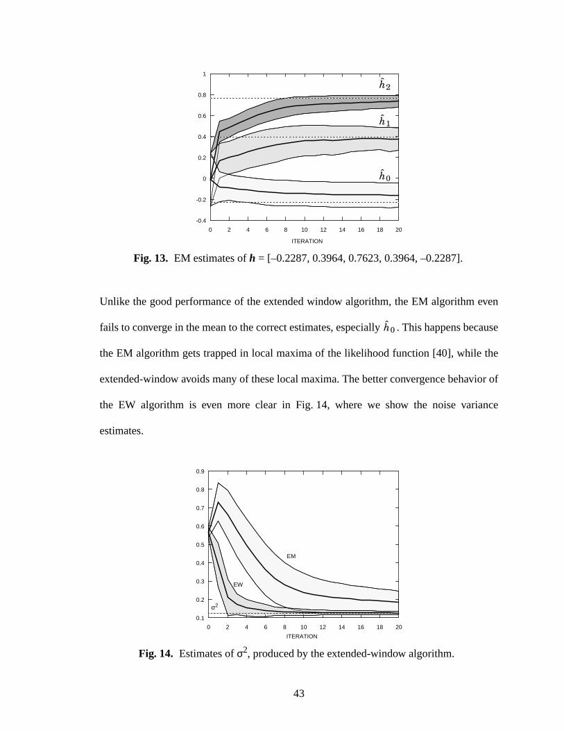
43

Unlike the good performance of the extended window algorithm, the EM algorithm even

fails to converge in the mean to the correct estimates, especially . This happens because

the EM algorithm gets trapped in local maxima of the likelihood function [40], while the

extended-window avoids many of these local maxima. The better convergence behavior of

the EW algorithm is even more clear in Fig. 14, where we show the noise variance

estimates.

ITERATION

Fig. 13. EM estimates of h = [–0.2287, 0.3964, 0.7623, 0.3964, –0.2287].

0 2 4 6 8 10 12 14 16 18 20

-0.4

-0.2

0

0.2

0.4

0.6

0.8

1

h2

h1

h0

h0

Fig. 14. Estimates of σ2, produced by the extended-window algorithm.

0 2 4 6 8 10 12 14 16 18 20

0.1

0.2

0.3

0.4

0.5

0.6

0.7

0.8

0.9

σ2

EW

EM

ITERATION

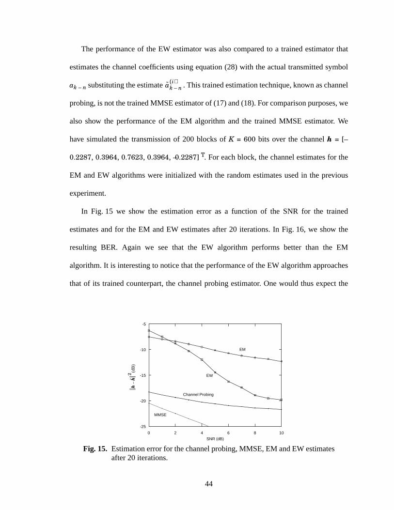
44

The performance of the EW estimator was also compared to a trained estimator that

estimates the channel coefficients using equation (28) with the actual transmitted symbol

ak – n substituting the estimate . This trained estimation technique, known as channel

probing, is not the trained MMSE estimator of (17) and (18). For comparison purposes, we

also show the performance of the EM algorithm and the trained MMSE estimator. We

have simulated the transmission of 200 blocks of K = 600 bits over the channel h = [–

0.2287, 0.3964, 0.7623, 0.3964, –0.2287] T. For each block, the channel estimates for the

EM and EW algorithms were initialized with the random estimates used in the previous

experiment.

In Fig. 15 we show the estimation error as a function of the SNR for the trained

estimates and for the EM and EW estimates after 20 iterations. In Fig. 16, we show the

resulting BER. Again we see that the EW algorithm performs better than the EM

algorithm. It is interesting to notice that the performance of the EW algorithm approaches

that of its trained counterpart, the channel probing estimator. One would thus expect the

ak n–i( )

Fig. 15. Estimation error for the channel probing, MMSE, EM and EW estimatesafter 20 iterations.

SNR (dB)

hh

–2 (d

B)

0 2 4 6 8 10

-25

-20

-15

-10

-5

MMSE

EW

EM

Channel Probing

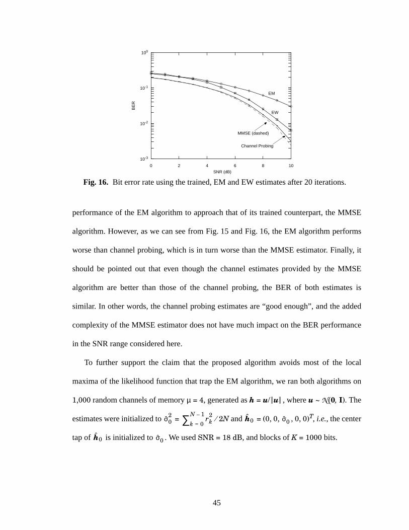
45

performanceof the EM algorithmto approachthat of its trainedcounterpart,the MMSE

algorithm.However, aswe canseefrom Fig. 15 andFig. 16, theEM algorithmperforms

worsethanchannelprobing,which is in turn worsethantheMMSE estimator. Finally, it

shouldbe pointedout that even thoughthe channelestimatesprovided by the MMSE

algorithm are better than thoseof the channelprobing, the BER of both estimatesis

similar. In otherwords,thechannelprobingestimatesare“good enough”,andtheadded

complexity of theMMSE estimatordoesnot have muchimpacton theBER performance

in the SNR range considered here.

To further supportthe claim that the proposedalgorithm avoids most of the local

maximaof the likelihoodfunctionthat traptheEM algorithm,we ranbothalgorithmson

1,000 randomchannelsof memoryµ = 4, generatedash = u/ , whereu ~ N(0, I). The

estimateswereinitializedto = ⁄ 2N and = (0, 0, , 0, 0)T, i.e., thecenter

tap of is initialized to . We usedSNR = 18 dB, and blocks ofK = 1000 bits.

Fig. 16. Bit errorrateusingthetrained,EM andEW estimatesafter20 iterations.

0 2 4 6 8 10

10-3

10-2

10-1

100

SNR (dB)

Channel Probing

EW

EM

BE

RMMSE (dashed)

u

σ02 rk

2k 0=

N 1–∑ h0 σ0

h0 σ0

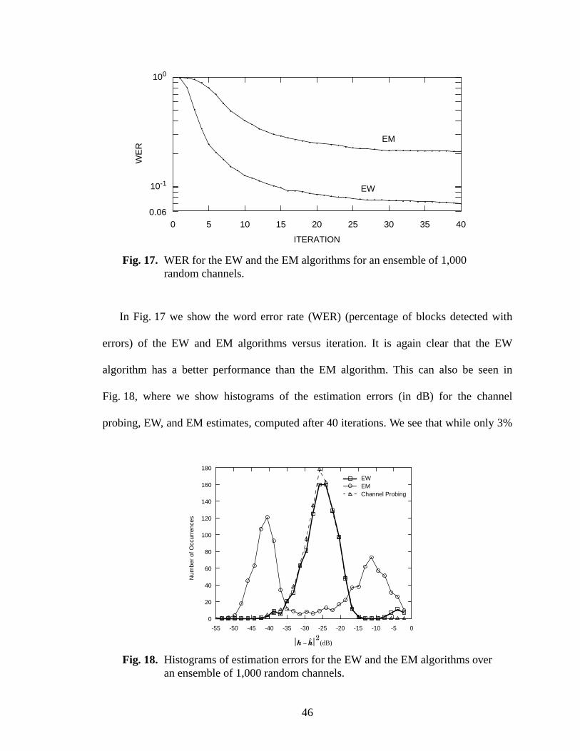
46

In Fig. 17 we show the word error rate (WER) (percentage of blocks detected with

errors) of the EW and EM algorithms versus iteration. It is again clear that the EW

algorithm has a better performance than the EM algorithm. This can also be seen in

Fig. 18, where we show histograms of the estimation errors (in dB) for the channel

probing, EW, and EM estimates, computed after 40 iterations. We see that while only 3%

Fig. 17. WER for the EW and the EM algorithms for an ensemble of 1,000random channels.

0 5 10 15 20 25 30 35 400.06

10-1

100

EW

EM

ITERATION

WE

R

Fig. 18. Histograms of estimation errors for the EW and the EM algorithms overan ensemble of 1,000 random channels.

h h–2

(dB)

-55 -50 -45 -40 -35 -30 -25 -20 -15 -10 -5 0

0

20

40

60

80

100

120

140

160

180

Channel ProbingEMEW

Num

ber

of O

ccur

renc

es

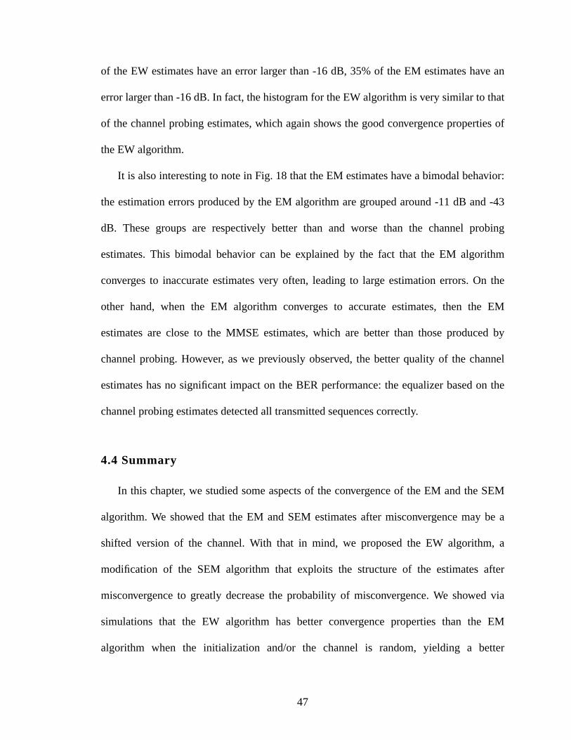
47

of the EW estimates have an error larger than -16 dB, 35% of the EM estimates have an

error larger than -16 dB. In fact, the histogram for the EW algorithm is very similar to that

of the channel probing estimates, which again shows the good convergence properties of

the EW algorithm.

It is also interesting to note in Fig. 18 that the EM estimates have a bimodal behavior:

the estimation errors produced by the EM algorithm are grouped around -11 dB and -43

dB. These groups are respectively better than and worse than the channel probing

estimates. This bimodal behavior can be explained by the fact that the EM algorithm

converges to inaccurate estimates very often, leading to large estimation errors. On the

other hand, when the EM algorithm converges to accurate estimates, then the EM

estimates are close to the MMSE estimates, which are better than those produced by

channel probing. However, as we previously observed, the better quality of the channel

estimates has no significant impact on the BER performance: the equalizer based on the

channel probing estimates detected all transmitted sequences correctly.

4.4 Summary

In this chapter, we studied some aspects of the convergence of the EM and the SEM

algorithm. We showed that the EM and SEM estimates after misconvergence may be a

shifted version of the channel. With that in mind, we proposed the EW algorithm, a

modification of the SEM algorithm that exploits the structure of the estimates after

misconvergence to greatly decrease the probability of misconvergence. We showed via

simulations that the EW algorithm has better convergence properties than the EM

algorithm when the initialization and/or the channel is random, yielding a better

48

performance both in terms of BER and channel estimation error. In simulations, we also

compared the performance of the EW algorithm to a system that estimates the channel

using channel probing and knowledge of the transmitted symbols. We showed that the

performance gap between the EW system and the one with training is surprisingly small.

It should be pointed out that the trained estimators used in this section are unrealistic,

since they assume knowledge of the whole transmitted sequence. Therefore, the gap

between the EW and trained estimates should be even smaller in a practical system.

49

CHAPTER 5

The Soft-Feedback Equalizer

In section 2.3, the EM algorithm was shown to have three problems: slow

convergence, misconvergence and high computational complexity, stemming from need to

compute and invert the a posteriori sample autocorrelation matrix defined in (19) and

from the use of the BCJR equalizer. In chapter 3, we proposed the SEM algorithm, which

converges faster than the EM algorithm and does not require matrix inversion. In

chapter 4, we proposed the EW algorithm, which decreases the probability of

misconvergence. In this chapter, we will address the remaining problem of the EM

algorithm: the complexity that results from using the BCJR algorithm for estimating the

transmitted symbol.

The SEM and EW algorithms are not intrinsically tied to the BCJR equalizer, and may

be used with any equalizer that produces soft symbol information. With that in mind, in

this chapter we propose the soft decision feedback equalizer with priors (SFE), a low

complexity alternative to the BCJR algorithm that retains many of its attractive features. In

particular, it outputs soft information in the form of an estimate of the a posteriori LLR. It

also exploits a priori information on the transmitted symbols, in the form a priori LLR λpk.

Thus, it is well suited for applications such as turbo equalization (where the a priori

probabilities are provided by the channel decoder), semi-blind systems (in which the a

Ra

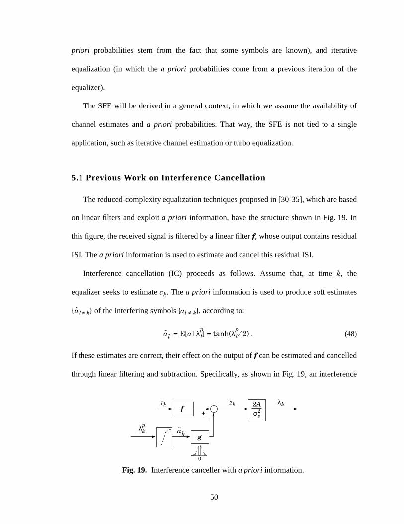
50

priori probabilities stem from the fact that some symbols are known), and iterative

equalization (in which the a priori probabilities come from a previous iteration of the

equalizer).

The SFE will be derived in a general context, in which we assume the availability of

channel estimates and a priori probabilities. That way, the SFE is not tied to a single

application, such as iterative channel estimation or turbo equalization.

5.1 Previous Work on Interference Cancellation

The reduced-complexity equalization techniques proposed in [30-35], which are based

on linear filters and exploit a priori information, have the structure shown in Fig. 19. In

this figure, the received signal is filtered by a linear filter f, whose output contains residual

ISI. The a priori information is used to estimate and cancel this residual ISI.

Interference cancellation (IC) proceeds as follows. Assume that, at time k, the

equalizer seeks to estimate ak. The a priori information is used to produce soft estimates

{ l ≠ k} of the interfering symbols {al ≠ k}, according to:

= E[a|λpl] = tanh(λ

pl ⁄ 2) . (48)

If these estimates are correct, their effect on the output of f can be estimated and cancelled

through linear filtering and subtraction. Specifically, as shown in Fig. 19, an interference

λk

Fig. 19. Interference canceller with a priori information.

f +–

0

g

rk

ak

zk

λpk

2Aσ2

v

a

al

51

cancellerfeedsthe soft decisionsthrough a filter g, whoseresponseis relatedto the

residualISI at theoutputof f. Sincetheequalizeroutputwill beusedto estimateak, the

influence of ak on the equalizeroutput should not be cancelled.Hence, the zero-th

coefficient of g is constrainedto be zero. The equalizersof [30-35] chooseg underthe

assumption that its input symbol estimates are correct, yieldinggk = ∑lhlfk – l whenk ≠ 0.

Sincethezero-thtapof g is zero, theequalizeroutputat time k, zk, is nota functionof

λpk. Thus, zk can only be usedto produceextrinsic information,which can be doneby

writing the equalizer output as

zk = Aak + vk, (49)

whereA = E[zkak] = ∑lhlf– l, andvk includestheeffect of channelnoiseandresidualISI.

Note that, from this definition,vk is independentof ak. The computationof the extrinsic

LLR λk from zk is easywhen vk is approximatedby a Gaussianrandomvariablewith

variance . In this case, we find that

λk = 2Azk ⁄ . (50)

The full LLR at the equalizer output is then given byLk = λk + λpk.

The equalizersproposedin [30] and [31], which we refer to as decision-aided

equalizers(DAE), choosef under the assumptionthat the soft decisionsof (48) are

correct,which leadsto thematched-filtersolutionfk = h–k . In theequalizersproposedin

[32,34] andin oneof thosein [35], f is anMMSE-LE. This equalizerdependson λpk and

must be recomputedevery time instantk, resulting in a time-varying equalizer(TVE)

whosecomputationalcomplexity is quadraticin thenumberof equalizercoefficients.Also

proposedin [32,35] are approximationsthat yield time-invariant filters f and g. In

σv2

σv2

52

particular, the switched-equalizer (SE) strategy proposed in [35] chooses f as either a

traditional MMSE equalizer or a matched filter (MF). A simple criterion to choose

between these two equalizers is proposed that depends on the quality of the a priori

information. In all cases [30-35], the cancellation filter g is designed under the assumption

that its input symbol estimates are correct, namely gk = ∑lhlfk – l for k ≠ 0.

5.2 The Soft-Feedback Equalizer

We now propose the SFE, a soft-output equalization scheme that shares many

similarities with the interference-cancellation schemes of [30-35]; however, our approach

differs in two substantial ways:

• At time k, when computing zk, the previous equalizer outputs {λk – j : j > 0} are

known. With these values, we may compute the full LLR Lk – j = λpk – j + λk – j,

which provides a better estimate of ak – j than λpk – j alone. Thus, instead of using

k – j to cancel interference, we propose to use k – j = E[ak – j|Lk – j] for j > 0.

This is similar in spirit to the principle behind a DFE. A DFE-based system is also

proposed in [35]. However, the system of [35] feeds back hard decisions on the

equalizer output, without combining them with the a priori information, and it per-

forms worse than the systems without feedback described in section 5.1. In [20], a

DFE was proposed to be used with a priori information. However, it does not use

the a priori information to cancel post-cursor ISI, and it computes the DFE coeffi-

cients assuming correct decisions.

• As in [32-35], instead of trying to cancel all the interference, we pass and

through linear filters whose coefficients, along with f, are computed to minimize

a a

ak ak

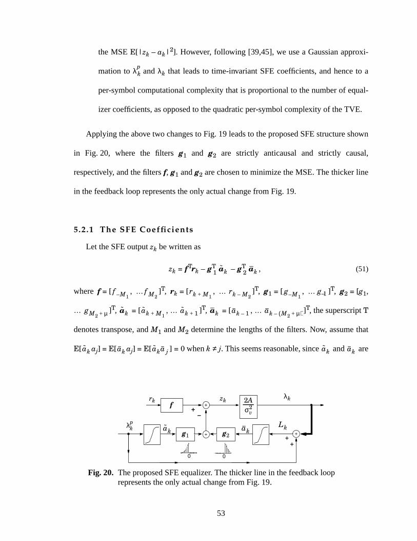
53

the MSE E[|zk – ak|2]. However, following [39,45], we use a Gaussian approxi-

mation to λpk and λk that leads to time-invariant SFE coefficients, and hence to a

per-symbol computational complexity that is proportional to the number of equal-

izer coefficients, as opposed to the quadratic per-symbol complexity of the TVE.

Applying the above two changes to Fig. 19 leads to the proposed SFE structure shown

in Fig. 20, where the filters g1 and g2 are strictly anticausal and strictly causal,

respectively, and the filters f, g1 and g2 are chosen to minimize the MSE. The thicker line

in the feedback loop represents the only actual change from Fig. 19.

5.2.1 The SFE Coefficients

Let the SFE output zk be written as

zk = fTrk – gT1 – gT

2 , (51)

where f = [ , … ]T, rk = [ , … ]T, g1 = [ , … g–1 ]T, g2 = [g1,

… ]T, = [ , … ]T, = [ , … ]T, the superscript T

denotes transpose, and M1 and M2 determine the lengths of the filters. Now, assume that

E[ aj] = E[ aj] = E[ ] = 0 when k ≠ j. This seems reasonable, since and are

λk

Fig. 20. The proposed SFE equalizer. The thicker line in the feedback looprepresents the only actual change from Fig. 19.

f +–

0

g2

rk

ak

zk

Lk

++

+–

g1ak

0

λpk

2Aσ2

v

ak ak

f M– 1f M2

rk M+ 1rk M2– g M– 1

gM2 µ+ ak ak M+ 1ak 1+ ak ak 1– ak M2 µ+( )–

ak ak aka j ak ak

54

approximately equal to ak and the transmitted symbols are uncorrelated. Then, as shown

in Appendix B, the values of f, g1 and g2 that minimize E[|zk – ak|2] are given by

f = (HHT – H1H1T – H2H2

T + σ2I)–1 h0 (52)

g1 = (α1 ⁄ E1) H1Tf (53)

g2 = (α2 ⁄ E2) H2Tf , (54)

where H is the M × (M + µ) channel convolution matrix:

H = , (55)

M = M1 + M2 + 1, and

E1 = E[| |2], (56)

E2 = E[| |2], (57)

α1 = E[ ak], (58)

α2 = E[ ak]. (59)

The vector h0 is the 0-th column of H, where the columns of H are numbered as H =

[ , … ]. Also, H1 = [ , … h–1 ] and H2 = [h1, … ]. The constants

A and , needed in (50) to compute the LLR λk from the equalizer output, are shown in

Appendix B to be given by A = fTh0 and = A (1 – A). Thus,

λk = 2 zk ⁄ (1 – fTh0). (60)

α12

E1-------

α22

E2-------

h0 h1 … hµ 0 0 … 0

0 h0 h1 … hµ 0 … 0

… … … … … … … …0 … … … h0 h1 … hµ

ak

ak

ak

ak

h M1– hM2 µ+ h M1– hM2 µ+

σv2

σv2

55

Note that, from the definitions of and , at time k we only attempt to cancel the

interference from the M1 future symbols and the M2 + µ past symbols. However,

rk = Ha k + nk, (61)

where nk = [ , … ]T and a k = [ , … ]T. Thus, the output of

the linear filter f suffers the interference of ak – j for j = – M1, … M2 + µ. In other words, at

time k the output of f has residual interference from the M1 future symbols and the

M2 + µ past symbols. This explains the index range in the definition of and . Also,

note that g1 and g2 are proportional to the strictly causal and anticausal portions of ∑lhlfk –

l, where the constants of proportionality depend on the quality of and through

α1 ⁄E1 and α2 ⁄E2.

5.2.2 Computing the Expected Values

Exploiting symmetries, it is not hard to see from (56)-(59) that E1, α1, E2 and α2 may

be computed by conditioning on ak = 1. In other words, E1 = E[| |2|ak = 1],

E2 = E[| |2|ak = 1], α1 = E[ |ak = 1], and α2 = E[ |ak = 1].

Now, assume that λpk is computed from an equivalent AWGN channel with output

lk = ak + wk, (62)

where wk is AWGN with variance , assumed to be independent of the transmitted

sequence, the actual channel noise and the equalizer output at time k [45]. Assuming a

BPSK alphabet, this means that λpk = γp lk, where γp = 2 ⁄ is proportional to the SNR of

the equivalent channel that generates λpk. Then, conditioning on ak = 1, λ

pk ~ N(γp, 2γp), so

α1 = ψ1(γp), (63)

E1 = ψ2(γp), (64)

ak ak

nk M+ 1nk M– 2

ak M+ 1ak M– 2 µ–

ak ak

ak ak

ak

ak ak ak

σw2

σw2

56

where

ψ1(γ) = E[tanh(u/2)], u ~ N(γ, 2γ), (65)

ψ2(γ) = E[tanh2(u/2)], u ~ N(γ, 2γ). (66)

Unfortunately, there are no closed-form formulas for ψ1(γ) and ψ2(γ). However, these are

well-behaved functions that may be tabulated or computed by simple numerical

algorithms.

Similarly, note that Lk = λpk + λk. Now, consider the Gaussian approximation to λk in

(49) and (50), and let γe = 2A2 ⁄ be a parameter that is proportional to the SNR of the

equivalent channel that generates λk. Then,

Lk = (γp + γe) ak + γpwk + γevk, (67)

so that, conditioning on ak = 1, Lk ~ N(γp + γe, 2 (γp + γe)). Thus, using the Gaussian

assumptions, E2 and α2 are given by

α2 = ψ1(γp + γe) (68)

E2 = ψ2(γp + γe). (69)

To compute E1, α1, E2 and α2, the values of γp and γe need to be estimated. Because

E[|λpk|

2] = + 2 γp, the ML estimate of γp is

= . (70)

To determine γe, we note that, as shown in Appendix B, A = fTh0 and = A (1 – A).

Thus, since γe = 2A2 ⁄ , we have that

γe = 2 fTh0 ⁄(1 – fTh0). (71)

σv2

γ p2

γ p 1 1N----- λk

p 2

k 0=

N 1–∑+ 1–

σv2

σv2

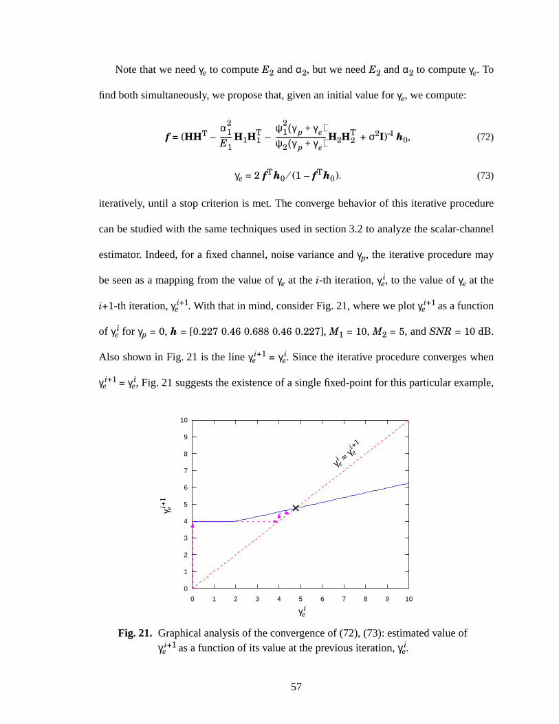
57

Note that we need γe to compute E2 and α2, but we need E2 and α2 to compute γe. To

find both simultaneously, we propose that, given an initial value for γe, we compute:

f = (HHT – H1H1T – H2H2

T + σ2I)–1 h0, (72)

γe = 2 fTh0 ⁄(1 – fTh0). (73)

iteratively, until a stop criterion is met. The converge behavior of this iterative procedure

can be studied with the same techniques used in section 3.2 to analyze the scalar-channel

estimator. Indeed, for a fixed channel, noise variance and γp, the iterative procedure may

be seen as a mapping from the value of γe at the i-th iteration, γei, to the value of γe at the

i+1-th iteration, γei+1. With that in mind, consider Fig. 21, where we plot γe

i+1 as a function

of γei for γp = 0, h = [0.227 0.46 0.688 0.46 0.227], M1 = 10, M2 = 5, and SNR = 10 dB.

Also shown in Fig. 21 is the line γei+1 = γe

i. Since the iterative procedure converges when

γei+1 = γe

i, Fig. 21 suggests the existence of a single fixed-point for this particular example,

α12

E1-------

ψ12 γ p γ e+( )

ψ2 γ p γ e+( )------------------------------

Fig. 21. Graphical analysis of the convergence of (72), (73): estimated value ofγe

i+1 as a function of its value at the previous iteration, γei.

0 1 2 3 4 5 6 7 8 9 10

0

1

2

3

4

5

6

7

8

9

10

γei

γ ei = γ e

i+1

γ ei+1

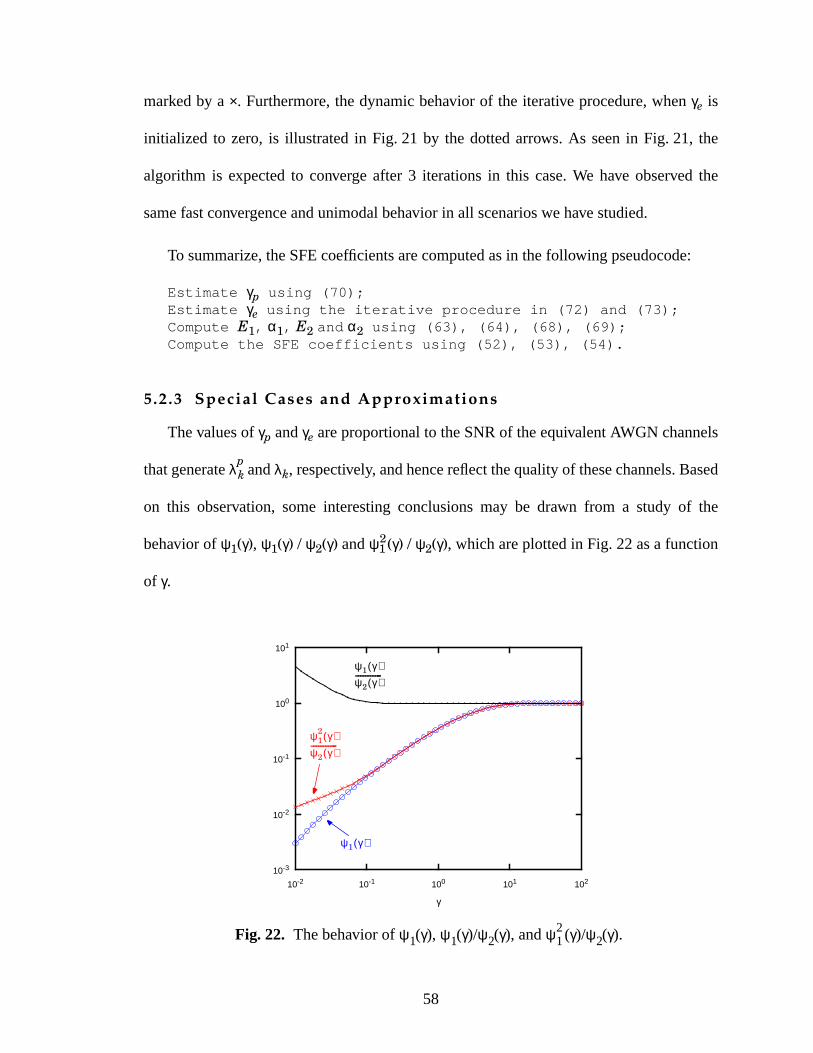
58

marked by a ×. Furthermore,the dynamicbehavior of the iterative procedure,whenγe is

initialized to zero, is illustratedin Fig. 21 by the dottedarrows. As seenin Fig. 21, the

algorithm is expectedto converge after 3 iterationsin this case.We have observed the

same fast convergence and unimodal behavior in all scenarios we have studied.

To summarize, the SFE coefficients are computed as in the following pseudocode:

Estimate γp using (70);Estimate γe using the iterative procedure in (72) and (73);Compute E1, α1, E2 and α2 using (63), (64), (68), (69);Compute the SFE coefficients using (52), (53), (54).

5.2.3 Special Cases and Approximations

Thevaluesof γp andγe areproportionalto theSNRof theequivalentAWGN channels

thatgenerateλpk andλk, respectively, andhencereflectthequalityof thesechannels.Based

on this observation, someinterestingconclusionsmay be drawn from a study of the

behavior of ψ1(γ), ψ1(γ) / ψ2(γ) andψ12(γ) / ψ2(γ), which areplottedin Fig. 22 asa function

of γ.

Fig. 22. The behavior of ψ1(γ), ψ1(γ)/ψ2(γ), andψ12(γ)/ψ2(γ).

10-2 10-1 100 101 10210-3

10-2

10-1

100

101

γ

ψ12 γ( )

ψ2 γ( )-----------

ψ1 γ( )

ψ1 γ( )ψ2 γ( )-----------

59

Consider, for instance, the case in which γp or γe tends to zero. It can be shown that, as

γ tends to zero, the ratio ψ1(γ) / ψ2(γ) tends to infinity, as suggested in Fig. 22. From

equations (53) and (54), this implies that the coefficients of the interference cancellers go

to infinity as the reliability of their inputs goes to zero. Hence, it seems that the less

reliable the symbol estimates, the more we try to cancel their interference. However, this

observation is not true. In fact, under the Gaussian assumption it is not hard to show that

the outputs of the interference cancellers are zero-mean random variables with variance

(α12 / E1) and (α2

2 / E2) . It is also possible to show that ψ12(γ) / ψ2(γ) tends

to zero as the reliability γ tends to zero, as suggested in Fig. 22. Thus, although the filter

coefficients grow large, the output of the interference canceller goes to zero in the mean-

square sense, and in fact no interference cancellation is done.

Based on Fig. 22, the analysis above, and a careful inspection of (52) – (54), it can be

shown that the SFE reduces to well-known equalizers for certain values of γp and γe.

• In the limit as γp and γe grow small, we have already shown that no IC is per-

formed. Furthermore, since ⁄ E1 → 0 as γp → 0 and ⁄ E2 → 0 as γe → 0, f

reduces to a traditional MMSE-LE. Therefore, in this case, the SFE reduces to a

conventional linear MMSE equalizer. This is intuitively pleasing, since small val-

ues of γp and γe suggest low levels of reliability, and in this case the receiver is bet-

ter off not attempting any form of interference cancellation.

• In the limit as γp → 0 and γe → ∞, the SFE reduces to a conventional MMSE-DFE.

This is intuitive, since small γp implies unreliable priors, and hence no cancellation

of precursor ISI should be performed. Furthermore, large γe implies reliable equal-

H1Tf

2H2

Tf2

α12 α2

2

60

izer outputs, in which case postcursor interference can be effectively cancelled

using decision-feedback.

• In the limit as γp → ∞, the SFE reduces to a traditional ISI canceller. This is intui-

tive because when γp is large, the equalizer has access to reliable estimates for all

interfering symbols. When the interfering symbols are known, the interference

canceller is known to be optimal.

The plot of ψ1(γ) / ψ2(γ) in Fig. 22 also indicates that we could replace α1 / E1 and α2 /

E2 by 1, an approximation that is clearly accurate for γ > 0.1. To analyze the effects of

this approximation for γ < 0.1, we observe that the feedforward filter f, as well as the

variance of the output of the interference cancellers, depend on α12 / E1 and α2

2 / E2. In

other words, we have to analyze the impact of the approximation on α12 / E1 and α2

2 / E2.

However, as suggested in Fig. 22, the difference between ψ1(γ) and ψ12(γ) / ψ2(γ) tends to

zero as γ tends to zero. Thus, α12 / E1 and α2

2 / E2 are close to α1 and α2, respectively, even

for unreliable channels. Therefore, approximating α1 / E1 and α2 / E2 by 1 does not

greatly affect the equalizer output. The resulting approximate filter coefficients are thus

computed as

f = (HHT – α1 H1H1T – α2 H2H2

T + σ2I)–1 h0, (74)

g1 = H1Tf, (75)

g2 = H2Tf. (76)

It is interesting to notice that, under this approximation, the coefficients of the interference

cancellers g1 and g2 are those that would be obtained assuming correct decisions. Thus,

the amount of interference cancellation to be performed by the equalizer is controlled

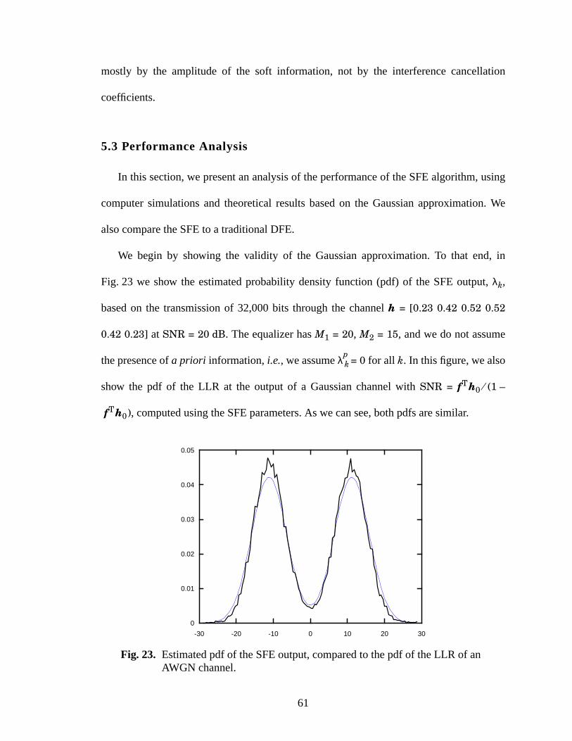
61

mostly by the amplitude of the soft information, not by the interference cancellation

coefficients.

5.3 Performance Analysis

In this section, we present an analysis of the performance of the SFE algorithm, using

computer simulations and theoretical results based on the Gaussian approximation. We

also compare the SFE to a traditional DFE.

We begin by showing the validity of the Gaussian approximation. To that end, in

Fig. 23 we show the estimated probability density function (pdf) of the SFE output, λk,

based on the transmission of 32,000 bits through the channel h = [0.23 0.42 0.52 0.52

0.42 0.23] at SNR = 20 dB. The equalizer has M1 = 20, M2 = 15, and we do not assume

the presence of a priori information, i.e., we assume λpk = 0 for all k. In this figure, we also

show the pdf of the LLR at the output of a Gaussian channel with SNR = fTh0 ⁄(1 –

fTh0), computed using the SFE parameters. As we can see, both pdfs are similar.

Fig. 23. Estimated pdf of the SFE output, compared to the pdf of the LLR of anAWGN channel.

-30 -20 -10 0 10 20 30

0

0.01

0.02

0.03

0.04

0.05

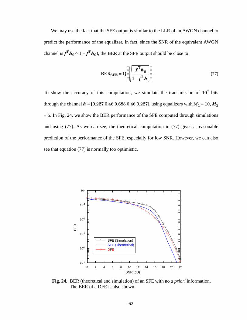
62

We may use the fact that the SFE output is similar to the LLR of an AWGN channel to

predict the performance of the equalizer. In fact, since the SNR of the equivalent AWGN

channel is fTh0 ⁄(1 – fTh0), the BER at the SFE output should be close to

BERSFE = Q . (77)

To show the accuracy of this computation, we simulate the transmission of 107 bits

through the channel h = [0.227 0.46 0.688 0.46 0.227], using equalizers with M1 = 10, M2

= 5. In Fig. 24, we show the BER performance of the SFE computed through simulations

and using (77). As we can see, the theoretical computation in (77) gives a reasonable

prediction of the performance of the SFE, especially for low SNR. However, we can also

see that equation (77) is normally too optimistic.

f Th0

1 f Th0–-----------------------

Fig. 24. BER (theoretical and simulation) of an SFE with no a priori information.The BER of a DFE is also shown.

0 2 4 6 8 10 12 14 16 18 20 22

10-5

10-4

10-3

10-2

10-1

100

SNR (dB)

BE

R

SFE (Simulation)SFE (Theoretical)DFE

63

In Fig. 24, we also show the BER performance of a DFE. It is interesting to notice that

as the SNR increases the performance of the DFE and the SFE become similar. This

agrees with the previous analysis, which predicted that the SFE becomes a DFE as the

SNR tends to infinity. It is also interesting to notice that the SFE outperforms the DFE for

SNR less than 8 dB, while the DFE is better than the SFE for SNR greater than 8 dB. This

indicates that, for this channel, there is an SNR threshold above which soft information

becomes too tentative, and the equalizer is better off using hard decisions. A similar

behavior was observed for other channels. In fact, our simulations indicate that if the SNR

at the SFE output, fTh0 ⁄(1 – fTh0), is greater than one, then the DFE performs better

than the SFE. Unfortunately, a theoretical computation of this SNR threshold could not be

determined for a general channel.

5.4 Summary

In this chapter, we proposed the SFE, a low-complexity soft-output equalizer that

exploits a priori information about the transmitted symbols to perform soft interference

cancellation. The SFE achieves a compromise between linear equalization, decision

feedback equalization and interference cancellation by choosing the equalizer coefficients

according to the quality of the priors and of the equalizer output. Since the SFE exploits a

priori information, it may replace the BCJR equalizer in applications.

The SFE differs from similar structures [30-35] in two ways. First, it successfully uses

soft feedback of the equalizer outputs to improve interference cancellation. In contrast, the

decision-feedback structure proposed in [35] performs worse than its linear counterpart.

64

Also, by assuming a statistical model for the priors, we obtain a time-invariant, linear

complexity equalizer, as opposed to the quadratic complexity of the MMSE structures in

[32-35].

We showed that the SFE collapses to well-known equalizers in limiting cases where

the a priori information and the equalizer output are very reliable or very unreliable. We

conducted simulations demonstrating the validity of the Gaussian approximation and

comparing the performance of the SFE to a DFE. In these simulations, we showed that the

SFE outperforms the DFE for low SNR. For high SNR, the performance of both equalizers

is similar. For the intermediate SNR range, the DFE outperforms the SFE, suggesting that

soft information may be too tentative for this SNR range, and better results are achieved

with hard information. This behavior was also observed in other simulations we conducted

for different channels, but we could not devise a general strategy to determine when hard

information yields better results than soft information.

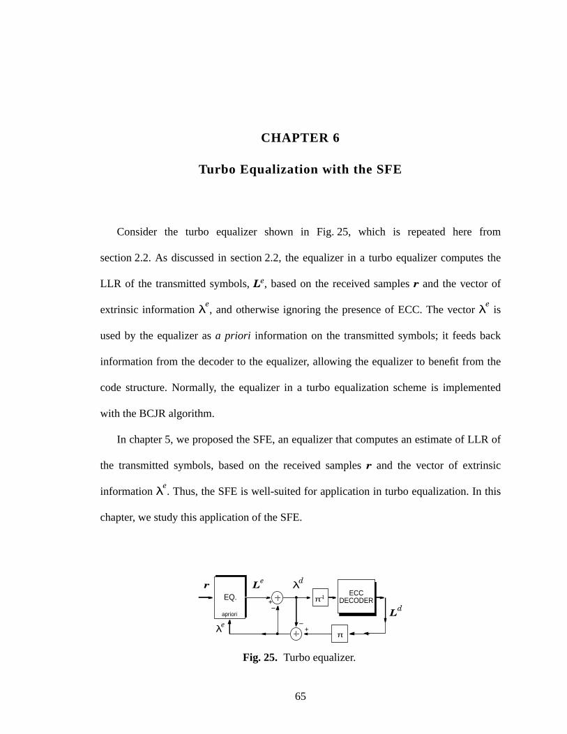
65

CHAPTER 6

Turbo Equalization with the SFE

Consider the turbo equalizer shown in Fig. 25, which is repeated here from

section 2.2. As discussed in section 2.2, the equalizer in a turbo equalizer computes the

LLR of the transmitted symbols, Le, based on the received samples r and the vector of

extrinsic information λe, and otherwise ignoring the presence of ECC. The vector λe

is

used by the equalizer as a priori information on the transmitted symbols; it feeds back

information from the decoder to the equalizer, allowing the equalizer to benefit from the

code structure. Normally, the equalizer in a turbo equalization scheme is implemented

with the BCJR algorithm.

In chapter 5, we proposed the SFE, an equalizer that computes an estimate of LLR of

the transmitted symbols, based on the received samples r and the vector of extrinsic

information λe. Thus, the SFE is well-suited for application in turbo equalization. In this

chapter, we study this application of the SFE.

Fig. 25. Turbo equalizer.

EQ.–

+

– +

apriori

ECCDECODERπ –1

π

λdLer

λeLd

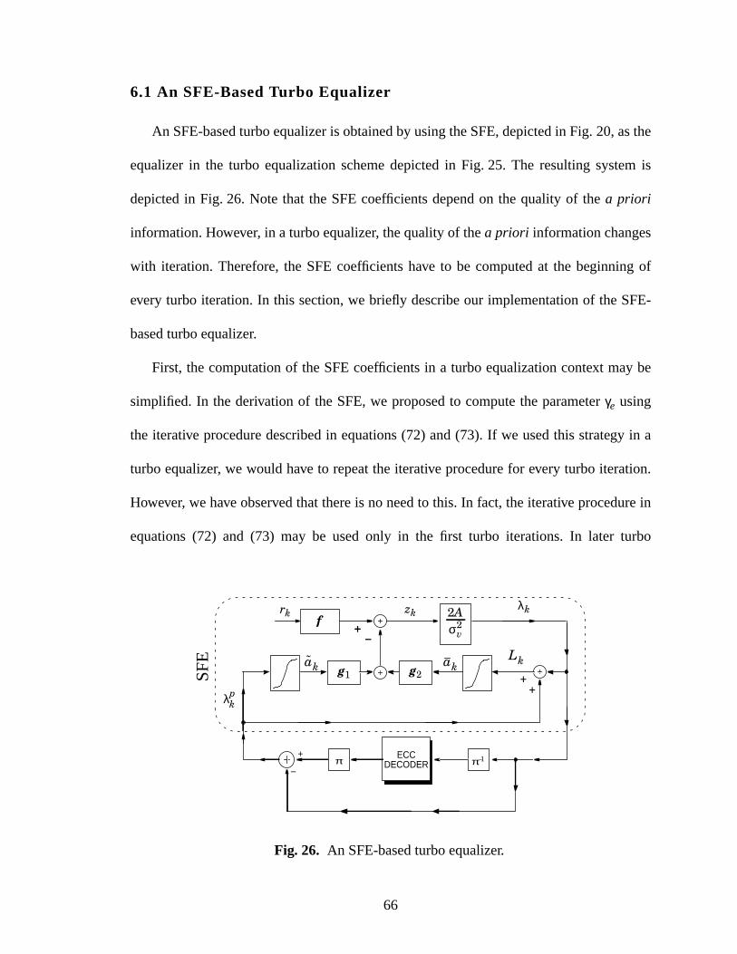
66

6.1 An SFE-Based Turbo Equalizer

An SFE-basedturboequalizeris obtainedby usingtheSFE,depictedin Fig. 20,asthe

equalizerin the turbo equalizationschemedepictedin Fig. 25. The resultingsystemis

depictedin Fig. 26. Note that the SFEcoefficientsdependon the quality of the a priori

information.However, in a turboequalizer, thequalityof thea priori informationchanges

with iteration.Therefore,the SFEcoefficientshave to be computedat the beginning of

every turbo iteration.In this section,we briefly describeour implementationof theSFE-

based turbo equalizer.

First, the computationof the SFEcoefficientsin a turbo equalizationcontext may be

simplified. In the derivation of the SFE,we proposedto computethe parameterγe using

the iterative proceduredescribedin equations(72) and(73). If we usedthis strategy in a

turboequalizer, we would have to repeatthe iterative procedurefor every turbo iteration.

However, we have observedthatthereis no needto this. In fact,theiterative procedurein

equations(72) and (73) may be usedonly in the first turbo iterations.In later turbo

λk

Fig. 26. An SFE-based turbo equalizer.

f +–

g2

rk

ak

zk

Lk

++

+–

g1ak

λpk

2Aσ2

v

–

+

ECCDECODER π –1π

SF

E

67

iterations, we may compute the equalizer coefficients using the value γe from the previous

turbo iteration. An updated value of γe is then computed and passed on to the next turbo

iteration. We have observed that no performance loss is incurred if the iterative procedure

in equations (72) and (73) is used only in the first turbo iteration.

Also, at the first turbo iteration when γp = 0, we get E1 = α1 = 0. To avoid the

indeterminate α1 ⁄E1 in (52) – (54), we artificially set E1 = 1, α1 = 0 for the initial

iteration. This is reasonable since, at the first iteration, we do not want to perform any IC

based on the a priori probabilities. In fact, algorithms based solely on IC often have a

problem at the first turbo iteration, when no a priori information is available. For example,

to solve this problem, [31] proposes that the BCJR algorithm be used for the first iteration.

Note that if we are using the approximate SFE coefficients in (74)-(76) the ratio α1 ⁄E1 is

never computed, so there is no need to artificially set E1 = 1, α1 = 0 for the initial iteration.

Finally, we have observed that a turbo equalizer may benefit from values of γp and γe

more pessimistic than those obtained using (70) and (71). Optimistic values for γp and γe

may cause the equalizer to output values of λk that have the wrong sign but a large

magnitude, which may cause the turbo equalizer to converge slowly or to a wrong

codeword. Performance can be improved if γp and γe are estimated using the SEM scalar

channel estimator analyzed in section 3.2, repeated here for convenience. If zk = Aak + vk

is the equalizer output, then, given initial estimates and , γe is computed iteratively

using

A0 σ02

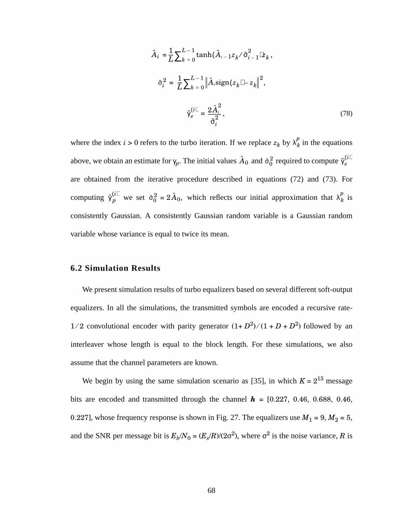
68

= ,

= ,

= , (78)

wherethe index i > 0 refersto the turbo iteration.If we replacezk by λpk in theequations

above,weobtainanestimatefor γp. Theinitial values and requiredto compute

are obtainedfrom the iterative proceduredescribedin equations(72) and (73). For

computing we set = 2 , which reflectsour initial approximationthat λpk is

consistentlyGaussian.A consistentlyGaussianrandomvariable is a Gaussianrandom

variable whose variance is equal to twice its mean.

6.2 Simulation Results

Wepresentsimulationresultsof turboequalizersbasedonseveraldifferentsoft-output

equalizers.In all the simulations,the transmittedsymbolsareencodeda recursive rate-

1 ⁄2 convolutional encoderwith parity generator(1+ D2) ⁄(1 + D + D2) followed by an

interleaver whoselength is equal to the block length. For thesesimulations,we also

assume that the channel parameters are known.

We begin by using the samesimulationscenarioas [35], in which K = 215 message

bits are encodedand transmittedthrough the channelh = [0.227, 0.46, 0.688, 0.46,

0.227], whosefrequency responseis shown in Fig. 27.TheequalizersuseM1 = 9, M2 = 5,

andtheSNRpermessagebit is Eb/N0 = (Es/R)/(2σ2), whereσ2 is thenoisevariance,R is

Ai1L---- tanh Ai 1– zk σi 1–

2⁄( )zkk 0=

L 1–∑

σi2 1

L---- Aisign zk( ) zk–

2

k 0=

L 1–∑

γ ei( ) 2 Ai

2

σi2

-----------------

A0 σ02 γ e

i( )

γ pi( )

σ02 A0

69

the code rate (in this case 1/2) and Es = is the symbol energy at the channel output.

We have estimated the BER performance as a function of Eb/N0 of turbo equalizers based

on the BCJR algorithm, the SFE, the time-varying equalizer (TVE) from [35], and the

switched equalizer (SE) from [35], after 14 iterations of the turbo equalizer. We have also

estimated the BER performance of the code in an AWGN channel, which does not

introduce ISI. The results, shown in Fig. 28, are averaged over 100 trials. As we can see,

the proposed equalizer performs almost as well as the TVE (quadratic complexity), while

its complexity is comparable to that of the SE (linear complexity).

In Fig. 28, it is also interesting to see that the performance of all the equalizers

eventually approaches that of the coded system in an AWGN channel. Thus, turbo

equalization allows for almost perfect ISI removal. In other words, for large enough SNR,

turbo systems may operate as if the channel introduced no ISI. Furthermore, in Fig. 28 we

show the capacity limit, defined as the minimum Eb/N0 required for error-free

Fig. 27. Frequency response of h = [0.227, 0.46, 0.688, 0.46, 0.227].

ω

|H(ω

)|2

(dB

)

-π -π/2 0 π/2 π-60

-50

-40

-30

-20

-10

0

10

h 2

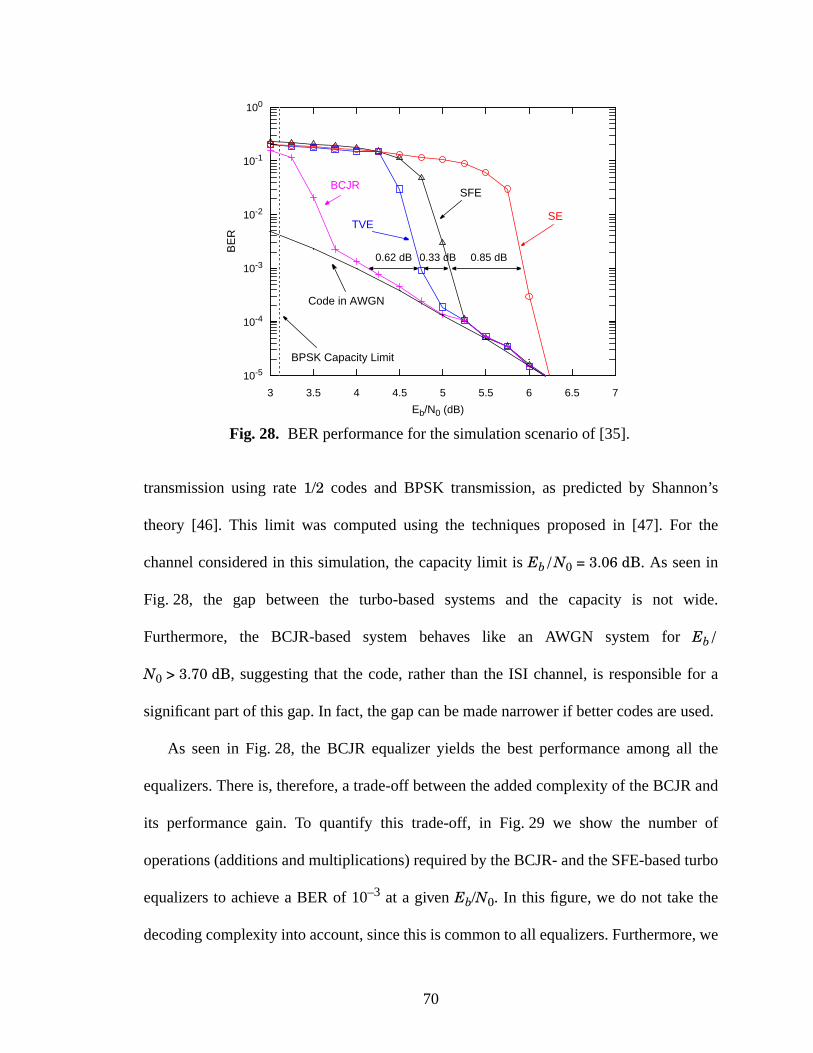
70

transmissionusing rate 1/2 codesand BPSK transmission,as predictedby Shannon’s

theory [46]. This limit was computedusing the techniquesproposedin [47]. For the

channelconsideredin this simulation,the capacitylimit is Eb/N0 = 3.06 dB. As seenin

Fig. 28, the gap between the turbo-basedsystems and the capacity is not wide.

Furthermore, the BCJR-basedsystem behaves like an AWGN system for Eb/

N0 > 3.70 dB, suggestingthat the code,ratherthanthe ISI channel,is responsiblefor a

significant part of this gap. In fact, the gap can be made narrower if better codes are used.

As seenin Fig. 28, the BCJR equalizeryields the bestperformanceamongall the

equalizers.Thereis, therefore,a trade-off betweentheaddedcomplexity of theBCJRand

its performancegain. To quantify this trade-off, in Fig. 29 we show the number of

operations(additionsandmultiplications)requiredby theBCJR-andtheSFE-basedturbo

equalizersto achieve a BER of 10–3 at a given Eb/N0. In this figure,we do not take the

decodingcomplexity into account,sincethis is commonto all equalizers.Furthermore,we

Fig. 28. BER performance for the simulation scenario of [35].

Eb/N0 (dB)

BE

RTVE

SFE

SE

BCJR

3 3.5 4 4.5 5 5.5 6 6.5 7

10-5

10-4

10-3

10-2

10-1

100

0.62 dB 0.33 dB 0.85 dB

Code in AWGN

BPSK Capacity Limit

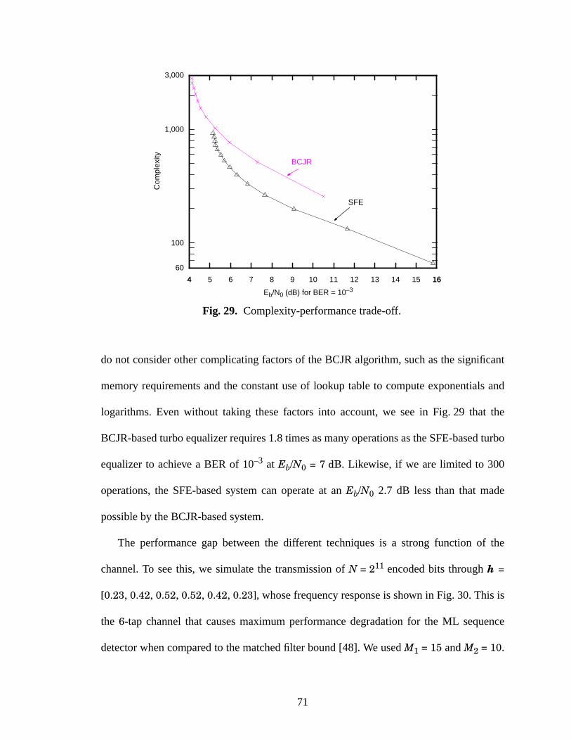
71

do not consider other complicating factors of the BCJR algorithm, such as the significant

memory requirements and the constant use of lookup table to compute exponentials and

logarithms. Even without taking these factors into account, we see in Fig. 29 that the

BCJR-based turbo equalizer requires 1.8 times as many operations as the SFE-based turbo

equalizer to achieve a BER of 10–3 at Eb/N0 = 7 dB. Likewise, if we are limited to 300

operations, the SFE-based system can operate at an Eb/N0 2.7 dB less than that made

possible by the BCJR-based system.

The performance gap between the different techniques is a strong function of the

channel. To see this, we simulate the transmission of N = 211 encoded bits through h =

[0.23, 0.42, 0.52, 0.52, 0.42, 0.23], whose frequency response is shown in Fig. 30. This is

the 6-tap channel that causes maximum performance degradation for the ML sequence

detector when compared to the matched filter bound [48]. We used M1 = 15 and M2 = 10.

Fig. 29. Complexity-performance trade-off.

Eb/N0 (dB) for BER = 10–3

Com

plex

ity

4 5 6 7 8 9 10 11 12 13 14 15 16

3,000

4 16

60

1,000

100

SFE

BCJR

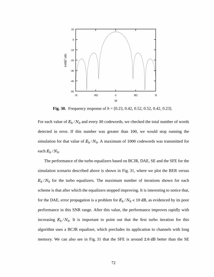
72

For each value of Eb ⁄ N0 and every 30 codewords, we checked the total number of words

detected in error. If this number was greater than 100, we would stop running the

simulation for that value of Eb ⁄ N0. A maximum of 1000 codewords was transmitted for

each Eb ⁄ N0.

The performance of the turbo equalizers based on BCJR, DAE, SE and the SFE for the

simulation scenario described above is shown in Fig. 31, where we plot the BER versus

Eb ⁄ N0 for the turbo equalizers. The maximum number of iterations shown for each

scheme is that after which the equalizers stopped improving. It is interesting to notice that,

for the DAE, error propagation is a problem for Eb ⁄ N0 < 10 dB, as evidenced by its poor

performance in this SNR range. After this value, the performance improves rapidly with

increasing Eb ⁄ N0. It is important to point out that the first turbo iteration for this

algorithm uses a BCJR equalizer, which precludes its application to channels with long

memory. We can also see in Fig. 31 that the SFE is around 2.6 dB better than the SE

Fig. 30. Frequency response of h = [0.23, 0.42, 0.52, 0.52, 0.42, 0.23].

-π -π/2 0 π/2 π-50

-40

-30

-20

-10

0

10

ω

|H(ω

)|2

(dB

)

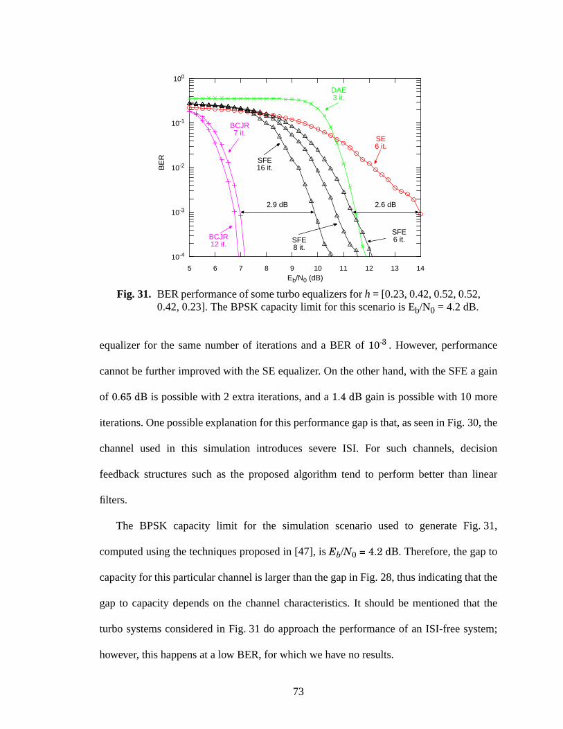
73

equalizer for the same number of iterations and a BER of 10–3 . However, performance

cannot be further improved with the SE equalizer. On the other hand, with the SFE a gain

of 0.65 dB is possible with 2 extra iterations, and a 1.4 dB gain is possible with 10 more

iterations. One possible explanation for this performance gap is that, as seen in Fig. 30, the

channel used in this simulation introduces severe ISI. For such channels, decision

feedback structures such as the proposed algorithm tend to perform better than linear

filters.

The BPSK capacity limit for the simulation scenario used to generate Fig. 31,

computed using the techniques proposed in [47], is Eb/N0 = 4.2 dB. Therefore, the gap to

capacity for this particular channel is larger than the gap in Fig. 28, thus indicating that the

gap to capacity depends on the channel characteristics. It should be mentioned that the

turbo systems considered in Fig. 31 do approach the performance of an ISI-free system;

however, this happens at a low BER, for which we have no results.

Fig. 31. BER performance of some turbo equalizers for h = [0.23, 0.42, 0.52, 0.52,0.42, 0.23]. The BPSK capacity limit for this scenario is Eb/N0 = 4.2 dB.

Eb/N0 (dB)

BE

R

DAE

SFE

SE

BCJR

6 it.

6 it.SFE8 it.

7 it.

BCJR12 it.

2.9 dB

3 it.

5 6 7 8 9 10 11 12 13 14

10-4

10-3

10-2

10-1

100

2.6 dB

SFE16 it.

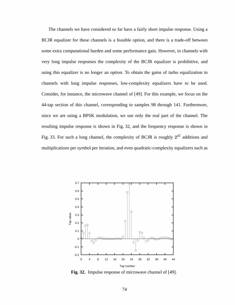
74

The channels we have considered so far have a fairly short impulse response. Using a

BCJR equalizer for these channels is a feasible option, and there is a trade-off between

some extra computational burden and some performance gain. However, in channels with

very long impulse responses the complexity of the BCJR equalizer is prohibitive, and

using this equalizer is no longer an option. To obtain the gains of turbo equalization in

channels with long impulse responses, low-complexity equalizers have to be used.

Consider, for instance, the microwave channel of [49]. For this example, we focus on the

44-tap section of this channel, corresponding to samples 98 through 141. Furthermore,

since we are using a BPSK modulation, we use only the real part of the channel. The

resulting impulse response is shown in Fig. 32, and the frequency response is shown in

Fig. 33. For such a long channel, the complexity of BCJR is roughly 247 additions and

multiplications per symbol per iteration, and even quadratic-complexity equalizers such as

Fig. 32. Impulse response of microwave channel of [49].

0 4 8 12 16 20 24 28 32 36 40 44

-0.2

-0.1

0

0.1

0.2

0.3

0.4

0.5

0.6

0.7

Tap number

Tap

val

ue

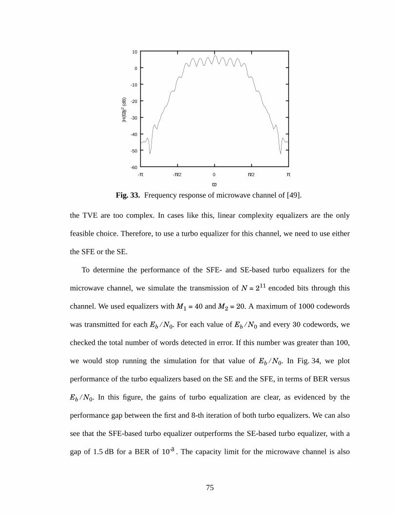
75

the TVE are too complex. In cases like this, linear complexity equalizers are the only

feasible choice. Therefore, to use a turbo equalizer for this channel, we need to use either

the SFE or the SE.

To determine the performance of the SFE- and SE-based turbo equalizers for the

microwave channel, we simulate the transmission of N = 211 encoded bits through this

channel. We used equalizers with M1 = 40 and M2 = 20. A maximum of 1000 codewords

was transmitted for each Eb ⁄N0. For each value of Eb ⁄N0 and every 30 codewords, we

checked the total number of words detected in error. If this number was greater than 100,

we would stop running the simulation for that value of Eb ⁄N0. In Fig. 34, we plot

performance of the turbo equalizers based on the SE and the SFE, in terms of BER versus

Eb ⁄N0. In this figure, the gains of turbo equalization are clear, as evidenced by the

performance gap between the first and 8-th iteration of both turbo equalizers. We can also

see that the SFE-based turbo equalizer outperforms the SE-based turbo equalizer, with a

gap of 1.5 dB for a BER of 10–3 . The capacity limit for the microwave channel is also

Fig. 33. Frequency response of microwave channel of [49].

-π -π/2 0 π/2 π

ω

|H(ω

)|2

(dB

)

-60

-50

-40

-30

-20

-10

0

10

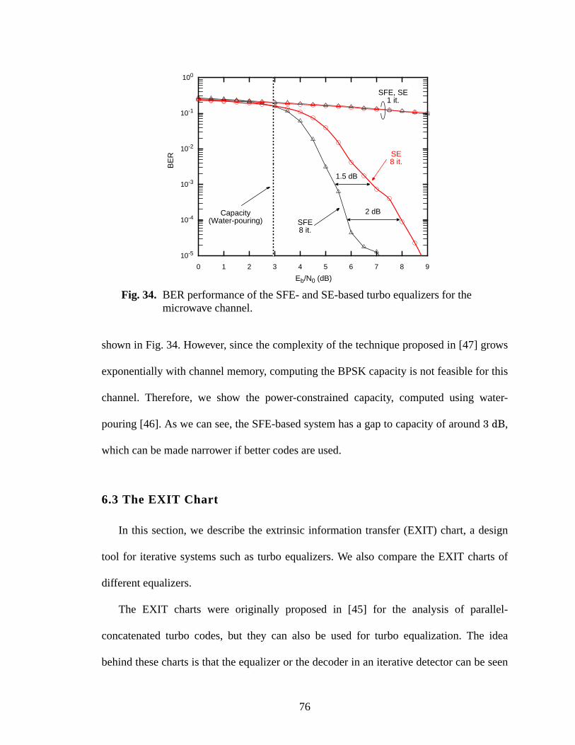
76

shown in Fig. 34. However, since the complexity of the technique proposed in [47] grows

exponentially with channel memory, computing the BPSK capacity is not feasible for this

channel. Therefore, we show the power-constrained capacity, computed using water-

pouring [46]. As we can see, the SFE-based system has a gap to capacity of around 3 dB,

which can be made narrower if better codes are used.

6.3 The EXIT Chart

In this section, we describe the extrinsic information transfer (EXIT) chart, a design

tool for iterative systems such as turbo equalizers. We also compare the EXIT charts of

different equalizers.

The EXIT charts were originally proposed in [45] for the analysis of parallel-

concatenated turbo codes, but they can also be used for turbo equalization. The idea

behind these charts is that the equalizer or the decoder in an iterative detector can be seen

Fig. 34. BER performance of the SFE- and SE-based turbo equalizers for themicrowave channel.

Eb/N0 (dB)

BE

R SE8 it.

SFE8 it.

0 1 2 3 4 5 6 7 8 9

10-5

10-4

10-3

10-2

10-1

100

SFE, SE1 it.

1.5 dB

2 dBCapacity(Water-pouring)

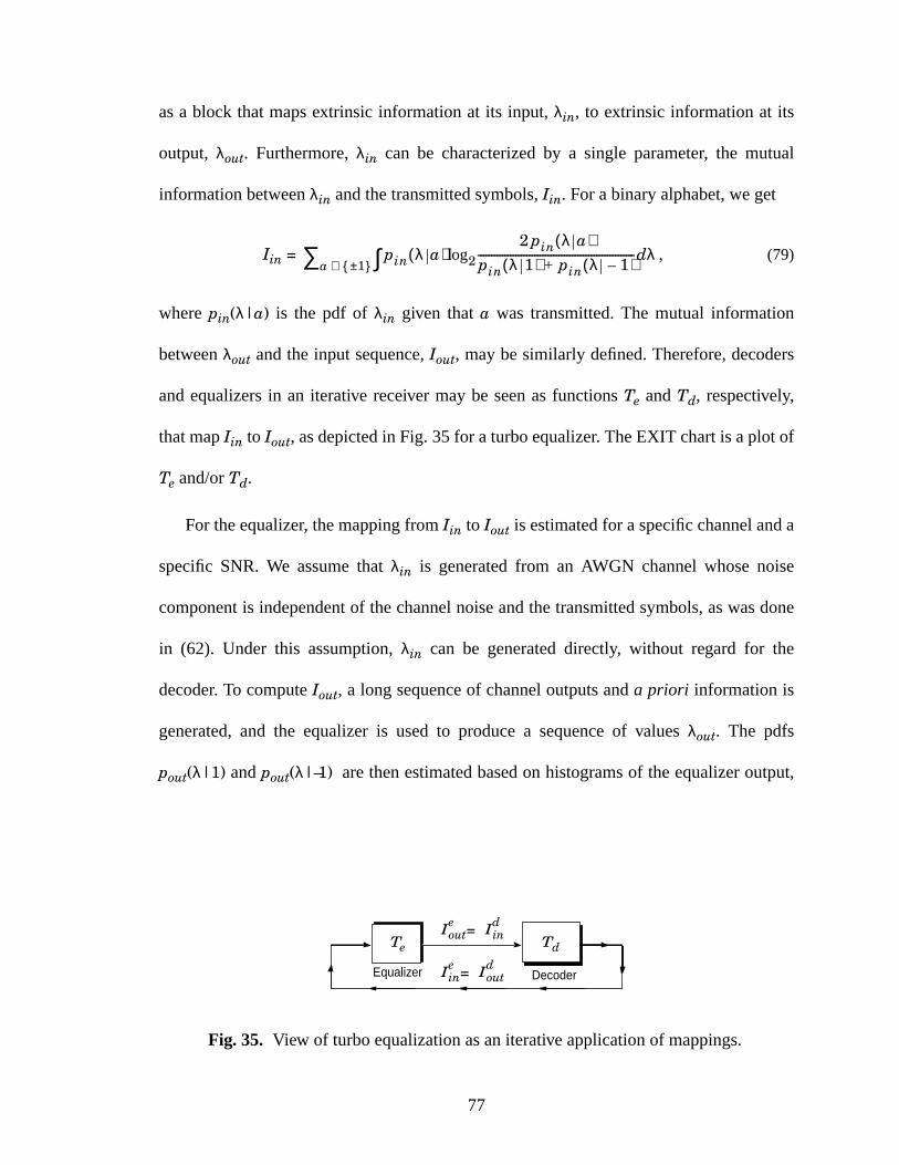
77

as a block that maps extrinsic information at its input, λin, to extrinsic information at its

output, λout. Furthermore, λin can be characterized by a single parameter, the mutual

information between λin and the transmitted symbols, Iin. For a binary alphabet, we get

Iin = , (79)

where pin(λ|a) is the pdf of λin given that a was transmitted. The mutual information

between λout and the input sequence, Iout, may be similarly defined. Therefore, decoders

and equalizers in an iterative receiver may be seen as functions Te and Td, respectively,

that map Iin to Iout, as depicted in Fig. 35 for a turbo equalizer. The EXIT chart is a plot of

Te and/or Td.

For the equalizer, the mapping from Iin to Iout is estimated for a specific channel and a

specific SNR. We assume that λin is generated from an AWGN channel whose noise

component is independent of the channel noise and the transmitted symbols, as was done

in (62). Under this assumption, λin can be generated directly, without regard for the

decoder. To compute Iout, a long sequence of channel outputs and a priori information is

generated, and the equalizer is used to produce a sequence of values λout. The pdfs

pout(λ|1) and pout(λ|–1) are then estimated based on histograms of the equalizer output,

pin λ a( )log22 pin λ a( )

pin λ 1( ) pin λ 1–( )+---------------------------------------------------------- λd∫a 1±{ }∈∑

Iein

Fig. 35. View of turbo equalization as an iterative application of mappings.

Ieout = Id

inTe Td

Equalizer DecoderIein = Id

out

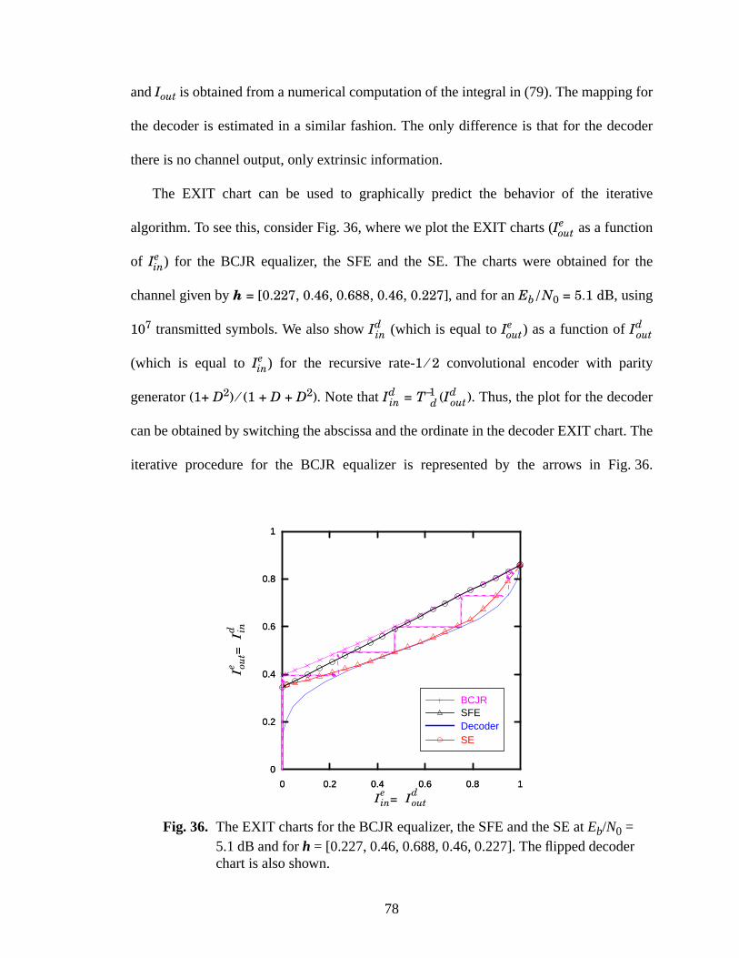
78

andIout is obtainedfrom anumericalcomputationof theintegral in (79).Themappingfor

the decoderis estimatedin a similar fashion.The only differenceis that for the decoder

there is no channel output, only extrinsic information.

The EXIT chart can be used to graphically predict the behavior of the iterative

algorithm.To seethis,considerFig. 36,wherewe plot theEXIT charts(Ieout asa function

of Iein) for the BCJR equalizer, the SFE and the SE. The chartswere obtainedfor the

channelgivenby h = [0.227, 0.46, 0.688, 0.46, 0.227], andfor anEb/N0 = 5.1 dB, using

107 transmittedsymbols.We alsoshow Idin (which is equalto Ie

out) asa function of Idout

(which is equal to Iein) for the recursive rate-1 ⁄2 convolutional encoderwith parity

generator(1+ D2) ⁄(1 + D + D2). NotethatIdin = T –1

d (Idout). Thus,theplot for thedecoder

canbeobtainedby switchingtheabscissaandtheordinatein thedecoderEXIT chart.The

iterative procedurefor the BCJR equalizer is representedby the arrows in Fig. 36.

Fig. 36. The EXIT charts for the BCJR equalizer, the SFE and the SE atEb/N0 =5.1dB andfor h = [0.227,0.46,0.688,0.46,0.227].Theflippeddecoderchart is also shown.

Iein = Id

out

Ie out =

Id in

SFEDecoderSE

BCJR

0 0.2 0.4 0.6 0.8 1

0

0.2

0.4

0.6

0.8

1

0 0.2 0.4 0.6 0.8 1

0

0.2

0.4

0.6

0.8

1

79

Initially, the equalizer has no extrinsic information, so that Iein = 0, so it produces an output

with Ieout = Te(0), represented by the first vertical arrow. The decoder then produces an

output with Iein = Td(Ie

out), a value that can be found graphically through the first horizontal

arrow. (Remember that for the decoder we plot Ieout = T –1

d (Iein).) With this new value of Ie

in,

the equalizer produces a new value Ieout = Te(I

ein), found with the second vertical arrow.

The iterative procedure progresses in the same fashion in future iterations.

As seen in Fig. 36, for both the BCJR equalizer and the SFE the mutual information

tends to a large value (close to 1) as the iterations progress, which implies a small BER

[45]. For the SE, however, the mutual information stops increasing at a small value, which

implies a large BER. Furthermore, we see that the BCJR-based turbo equalizer is expected

to converge in 5 iterations, while the SFE-based turbo equalizer is expected to converge in

6 iterations. Finally, we see in Fig. 36 that for no extrinsic information (Iein = 0) the SFE

produces the same Ieout as the SE. However, when Ie

in = 0 the SE chooses the MMSE-LE.

These two observations indicate that the SFE performs like an MMSE-LE. This is

intuitively pleasing, since in the absence of a priori information and with unreliable

equalizer outputs (caused by the low SNR), the SFE should indeed be similar to an

MMSE-LE. We can also see in Fig. 36 that, as the reliability of the extrinsic information

increases, the SFE, the SE and the BCJR equalizer produce the same Ieout. This agrees with

the analysis in section 5.2.3 that showed that when the reliability of the extrinsic

information tends to infinity, the SFE tends to an MF with IC, which is the ML receiver in

this case. (Remember that the SE is an MF when the a priori information is reliable.)

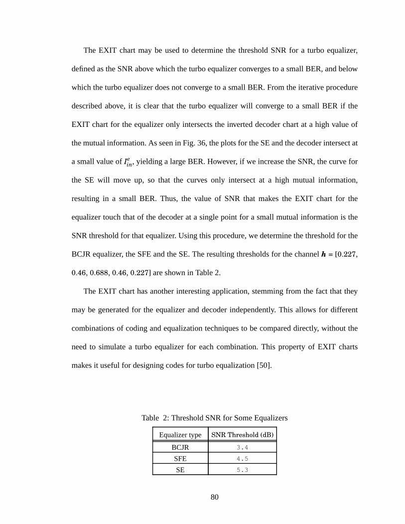
80

The EXIT chart may be used to determine the threshold SNR for a turbo equalizer,

defined as the SNR above which the turbo equalizer converges to a small BER, and below

which the turbo equalizer does not converge to a small BER. From the iterative procedure

described above, it is clear that the turbo equalizer will converge to a small BER if the

EXIT chart for the equalizer only intersects the inverted decoder chart at a high value of

the mutual information. As seen in Fig. 36, the plots for the SE and the decoder intersect at

a small value of Iein, yielding a large BER. However, if we increase the SNR, the curve for

the SE will move up, so that the curves only intersect at a high mutual information,

resulting in a small BER. Thus, the value of SNR that makes the EXIT chart for the

equalizer touch that of the decoder at a single point for a small mutual information is the

SNR threshold for that equalizer. Using this procedure, we determine the threshold for the

BCJR equalizer, the SFE and the SE. The resulting thresholds for the channel h = [0.227,

0.46, 0.688, 0.46, 0.227] are shown in Table 2.

The EXIT chart has another interesting application, stemming from the fact that they

may be generated for the equalizer and decoder independently. This allows for different

combinations of coding and equalization techniques to be compared directly, without the

need to simulate a turbo equalizer for each combination. This property of EXIT charts

makes it useful for designing codes for turbo equalization [50].

Table 2: Threshold SNR for Some Equalizers

Equalizer type SNR Threshold (dB)

BCJR 3.4

SFE 4.5

SE 5.3

81

6.4 Summary

In this chapter, we studied the application of the SFE for turbo equalization. We first

proposed some modifications to the computation of the SFE coefficients that reduce the

computational complexity of the system and improve its performance. We then showed,

through simulations, that an SFE-based turbo equalizer may perform within 1 dB of a

BCJR-based turbo equalizer, which has exponential complexity in the memory of the

channel, and within 0.4 dB of a TVE-based turbo equalizer, which has quadratic

complexity in the memory of the channel. We showed that the SFE-based turbo equalizer

consistently outperforms turbo equalizers based on other linear complexity equalizers.

We have also discussed EXIT charts, a tool for the design of iterative systems. We

have provided the EXIT charts of the SFE and compared them with the charts for the

BCJR equalizer and the SE. As expected, the SFE is seen to perform between the SE and

the BCJR equalizer.

82

CHAPTER 7

ECC-Aware Blind Channel Estimation

As we have discussed so far, the principle behind the success of iterative techniques is

that of exchanging information between blocks so that at every iteration each block uses

information from other blocks to improve the reliability of its output. Within that

philosophy, in this chapter we combine turbo equalizers and iterative channel estimators in

a single system in which channel estimation is based on the decoder output instead of the

equalizer output. This way the channel estimator benefits from the code structure, which

makes the decoder output more reliable than that of the equalizer, resulting in a blind

iterative ECC-aware channel estimator. In a way, this is not very different from the EW

channel estimator of chapter 4, since the combination of an equalizer and a decoder can be

seen as a symbol estimator.

7.1 ECC-Aware Blind Estimation of a Scalar Channel

In this section, we explain the idea behind ECC-aware channel estimation in simple

terms, by considering a scalar channel as shown in Fig. 37. Given initial estimates 0 and

, the ECC-ignorant approach to estimating the channel gain A and the noise variance σ2

computes:

A

σ02

83

i + 1 = rk tanh( irk/ ), (80)

= |rk – sign(rk) i + 1|2. (81)

The idea behind these equations is that 2 irk/ is an estimate of the LLR of the channel

input ak, which is equal to 2Ark / σ2 if only the channel is taken into account. We may,

however, obtain a better estimate for this LLR by taking the code into account. This can be

done by considering the output of the BCJR decoder. In this case, we may estimate

i + 1 = rk tanh(λk/2), (82)

= |rk – sign(λk) i + 1|2. (83)

7.2 ECC-Aware Blind Estimation of an ISI Channel

In this section, we propose an ECC-aware blind channel estimator for a general

channel. The application of the principle discussed in the previous section to a channel

that introduces ISI is not straightforward. After all, when discussing turbo equalization,

we saw that it is hard to obtain the APP on the transmitted symbols while taking the code

structure into account. However, we also saw that turbo equalizers may produce an

approximation to this APP. In fact, one important aspect of turbo equalizers is that they

λk

Fig. 37. A simple encoded scalar channel.

Channel

A

m

pa

P(D) to B

PSK r

ECC ENCODERDecoder

AWGNm

Gain

BCJR

A 1N-----

k 0=

N 1–∑ A σi2

σi 1+2 1

N-----

k 0=

N 1–∑ A

A σi2

A 1N-----

k 0=

N 1–∑

σi 1+2 1

N-----

k 0=

N 1–∑ A

84

provide soft estimates of the transmitted sequence that benefit from the ECC code

structure, and are much more reliable than the estimates provided by an equalizer alone.

Its seems natural that using this information for channel estimation should provide better

results than using ECC-ignorant symbol estimates, as is done in Fig. 5. Thus, we propose

the channel estimator of Fig. 38, in which the symbol estimator in Fig. 5 is replaced by the

turbo equalizer of Fig. 3.

The proposed estimator of Fig. 38 iterates between three blocks: a channel estimator, a

soft-output equalizer, and a soft-output ECC decoder. A receiver would have to perform

these functions anyway, so their presence alone does not imply any added complexity; the

only added complexity is due to the fact that these functions are performed multiple times

as the algorithm iterates.

It is instructive to compare the proposed estimator with a conventional receiver that

performs channel estimation just once, then uses these estimates in a turbo equalizer. The

proposed estimator can be derived from this receiver by making just one modification:

EQ.

–

+

–+

apriori

ECCDECODER

a

ChannelEstimator

h

r

π –1

π

σ,

Fig. 38. Integrating channel estimation with turbo equalization.

Turbo Equalizer

λek

Lek

λdk

Ldk

(Symbol Estimator)

85

rather than using the initial channel estimates for every turbo iteration, the proposed

receiver occasionally improves the channel estimates based on tentative soft decisions.

Specifically, every J-th iteration of the turbo equalizer, the soft-symbol estimates

produced by the ECC decoder are used by the EW algorithm to produce better channel

estimates, which are then used for the next J iterations. Key to the good performance is the

fact that the a priori information for the turbo equalizer is not initialized to zero after J

iterations of the turbo equalizer. Instead, extrinsic information from the last instance is

used as the initial a priori information in the next one. The choice of J is a design

parameter that can affect convergence speed, steady-state behavior, and overall

complexity. Because of the low complexity of the channel estimator relative to the

complexity of the equalizer and ECC decoder, we have found empirically that J = 1 is a

reasonable choice. With this choice, each time the ECC decoder passes extrinsic

information to the equalizer, the channel estimates are simultaneously improved. This is

only marginally more complex than a conventional receiver that uses turbo equalization,

but the performance improvement that results can be significant.

One complicating factor for ECC-aware blind channel estimators is the presence of the

interleaver. As is well-known [7], the output of a blind equalizer, or of an equalizer based

on a blind estimator, is a delayed version of the channel input, and this delay cannot be

compensated for blindly. However, if a delayed sequence is fed to the deinterleaver in

Fig. 38, the decoder input will be practically independent of the encoder output. In this

case, the decoder output will also be practically independent of the channel input, so that

the channel estimates are almost zero. Thus, if a delay is present the blind ECC-aware

channel estimator fails. As seen in chapter 4, the EW algorithm exploits the knowledge of

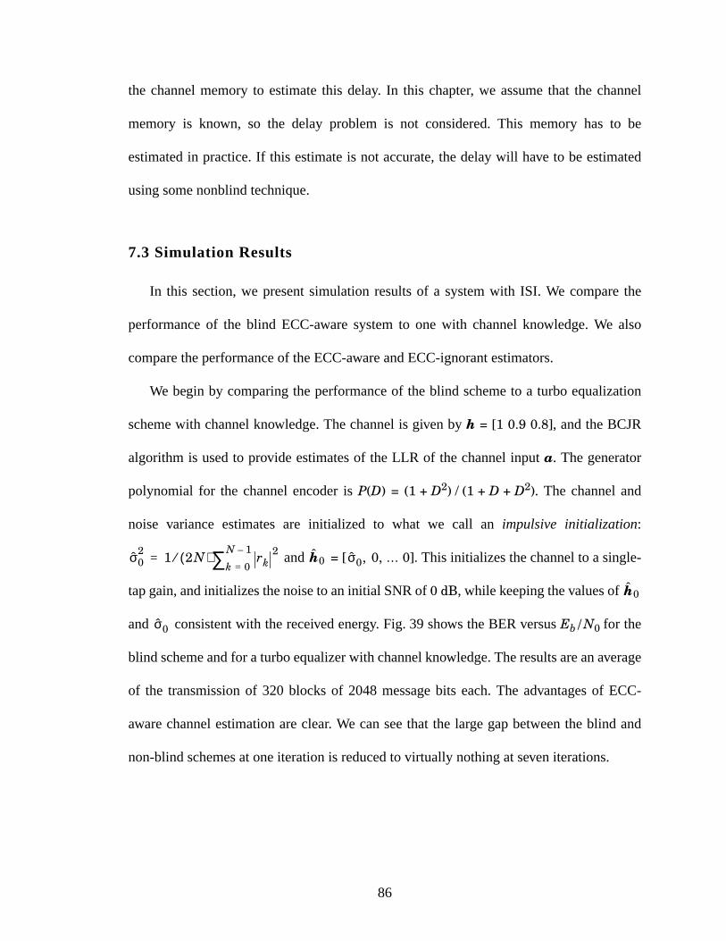
86

the channel memory to estimate this delay. In this chapter, we assume that the channel

memory is known, so the delay problem is not considered. This memory has to be

estimated in practice. If this estimate is not accurate, the delay will have to be estimated

using some nonblind technique.

7.3 Simulation Results

In this section, we present simulation results of a system with ISI. We compare the

performance of the blind ECC-aware system to one with channel knowledge. We also

compare the performance of the ECC-aware and ECC-ignorant estimators.

We begin by comparing the performance of the blind scheme to a turbo equalization

scheme with channel knowledge. The channel is given by h = [1 0.9 0.8], and the BCJR

algorithm is used to provide estimates of the LLR of the channel input a. The generator

polynomial for the channel encoder is P(D) = (1 + D2) / (1 + D + D2). The channel and

noise variance estimates are initialized to what we call an impulsive initialization:

and = [ , 0, … 0]. This initializes the channel to a single-

tap gain, and initializes the noise to an initial SNR of 0 dB, while keeping the values of

and consistent with the received energy. Fig. 39 shows the BER versus Eb/N0 for the

blind scheme and for a turbo equalizer with channel knowledge. The results are an average

of the transmission of 320 blocks of 2048 message bits each. The advantages of ECC-

aware channel estimation are clear. We can see that the large gap between the blind and

non-blind schemes at one iteration is reduced to virtually nothing at seven iterations.

σ02 1 2N( )⁄ rk

2k 0=

N 1–∑= h0 σ0

h0

σ0

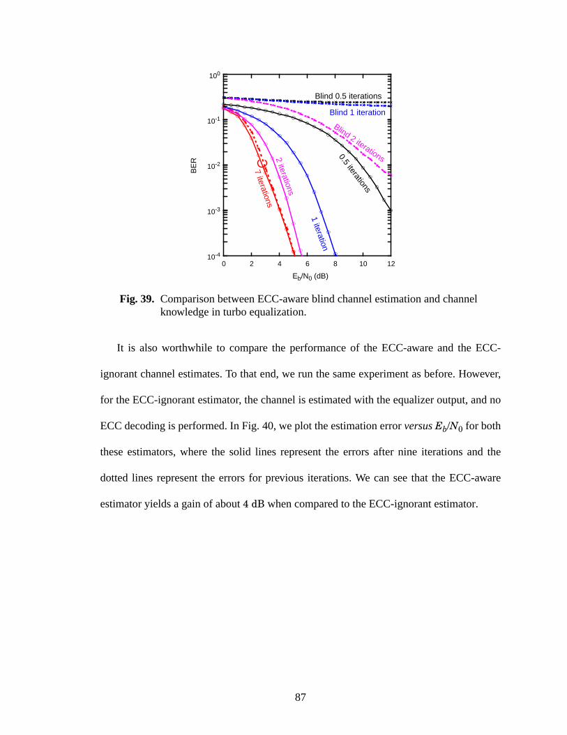
87

It is also worthwhile to compare the performance of the ECC-aware and the ECC-

ignorant channel estimates. To that end, we run the same experiment as before. However,

for the ECC-ignorant estimator, the channel is estimated with the equalizer output, and no

ECC decoding is performed. In Fig. 40, we plot the estimation error versus Eb/N0 for both

these estimators, where the solid lines represent the errors after nine iterations and the

dotted lines represent the errors for previous iterations. We can see that the ECC-aware

estimator yields a gain of about 4 dB when compared to the ECC-ignorant estimator.

Fig. 39. Comparison between ECC-aware blind channel estimation and channelknowledge in turbo equalization.

Eb/N0 (dB)

BE

R

0 2 4 6 8 10 1210-4

10-3

10-2

10-1

100

Blind 0.5 iterations

0.5 iterations

1 iteration

Blind 1 iteration

2 iterations

Blind 2 iterations

7 iterations

88

7.4 Study of Convergence

To studythe convergenceof the ECC-awarechannelestimator, andto compareit to

the ECC-ignorantestimator, we will use both thesealgorithms to estimaterandomly

generatedchannels.We declarea channel to be successfullyestimatedif the turbo

equalizerbasedontheseestimatescorrectlydetectsthetransmittedcodeword,withoutany

errors.

By defininga successfulchannelestimateasthatwhich yieldsno errors,anattemptto

estimatea channelmay fail not becauseof an intrinsic convergenceproblemwith the

estimationalgorithm,but ratherbecauseof misconvergenceof theturboequalizer. In fact,

it is known thatthereare“bad” sequencesfor a turbosystem,whichcausemany detection

errors.For example,in thetransmissionof say1,000informationbits with a BER of 10–3

Fig. 40. Comparison between ECC-aware and ECC-ignorant blind channelestimation.

Eb/N0 (dB)

2 (dB

)

ECC-awareECC-ignorant

hh

–

-4 -3 -2 -1 0 1 2 3 4 5 6

-30

-25

-20

-15

-10

-5

0

5

89

usingturbodetection,oneis not to expectonebit errorateveryblock,but ratheroneblock

with around200 bit errorsevery 200 blocks.In otherwords,someof the failuresin the

randomchannelexperimentare due to these“bad” channeloutputs,not to an inherent

convergenceproblemwith theblind channelestimator. In thatsense,wemustcomparethe

success of the blind algorithm with the success of the algorithm with channel knowledge.

We basedour analysison the randomchannelexperiment,in which a set of 400

informationbits weregeneratedandencodedusinga rate1/4 seriallyconcatenatedturbo

code consisting of two recursive systematic convolutional codes with generator

polynomialP(D) = (1 + D) / (1 + D + D2), andan interleaver betweenthe encoders.The

resulting encodedsequencewas then interleaved and transmittedthrough a 5-tap ISI

channel. We have conducted 1,000 such experiments, in which the channel, the

transmittedand noise sequences,and the interleavers were generatedrandomly. The

channelcoefficients in particularare generatedaccordingto h ~ N(0,I). The signal to

noiseratio waskeptconstantat Eb/N0 = 2 dB. Thenoisevarianceandchannelestimates

were initialized with an impulsive initialization.

For the ECC-ignorant case, we obviously cannot expect that the WER after

equalizationbe zero.However, we may usethe estimatesprovided by the ECC-ignorant

estimatorin aturboequalizationsetting.In thiscase,thechannelestimatesarenotupdated

astheturboequalizeriterates.WemaythenconsideranECC-ignorantchannelestimateto

besuccessfulif theturboequalizerbasedon this estimateproduceszeroerrors.Thus,the

successof the ECC-ignorantestimatorwas measuredby running a turbo equalizerthat

usesECC-ignorantestimates,whichwereobtainedafter30 iterationsof theECC-ignorant

channelestimator. In Fig. 41 we plot the word-errorrate(WER) versus iterationfor the

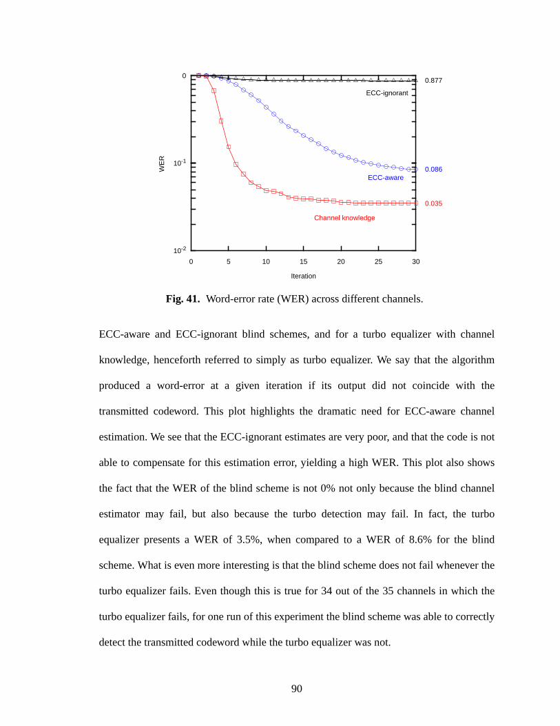
90

ECC-aware and ECC-ignorant blind schemes, and for a turbo equalizer with channel

knowledge, henceforth referred to simply as turbo equalizer. We say that the algorithm

produced a word-error at a given iteration if its output did not coincide with the

transmitted codeword. This plot highlights the dramatic need for ECC-aware channel

estimation. We see that the ECC-ignorant estimates are very poor, and that the code is not

able to compensate for this estimation error, yielding a high WER. This plot also shows

the fact that the WER of the blind scheme is not 0% not only because the blind channel

estimator may fail, but also because the turbo detection may fail. In fact, the turbo

equalizer presents a WER of 3.5%, when compared to a WER of 8.6% for the blind

scheme. What is even more interesting is that the blind scheme does not fail whenever the

turbo equalizer fails. Even though this is true for 34 out of the 35 channels in which the

turbo equalizer fails, for one run of this experiment the blind scheme was able to correctly

detect the transmitted codeword while the turbo equalizer was not.

Fig. 41. Word-error rate (WER) across different channels.

0 5 10 15 20 25 30

10-2

10-1

0

Iteration

WE

R

Channel knowledge

ECC-aware

ECC-ignorant

0.035

0.086

0.877

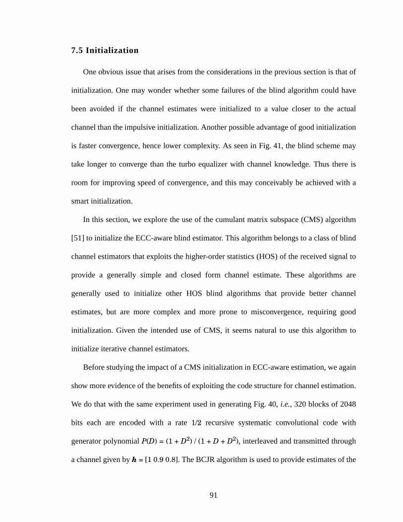
91

7.5 Initialization

One obvious issue that arises from the considerations in the previous section is that of

initialization. One may wonder whether some failures of the blind algorithm could have

been avoided if the channel estimates were initialized to a value closer to the actual

channel than the impulsive initialization. Another possible advantage of good initialization

is faster convergence, hence lower complexity. As seen in Fig. 41, the blind scheme may

take longer to converge than the turbo equalizer with channel knowledge. Thus there is

room for improving speed of convergence, and this may conceivably be achieved with a

smart initialization.

In this section, we explore the use of the cumulant matrix subspace (CMS) algorithm

[51] to initialize the ECC-aware blind estimator. This algorithm belongs to a class of blind

channel estimators that exploits the higher-order statistics (HOS) of the received signal to

provide a generally simple and closed form channel estimate. These algorithms are

generally used to initialize other HOS blind algorithms that provide better channel

estimates, but are more complex and more prone to misconvergence, requiring good

initialization. Given the intended use of CMS, it seems natural to use this algorithm to

initialize iterative channel estimators.

Before studying the impact of a CMS initialization in ECC-aware estimation, we again

show more evidence of the benefits of exploiting the code structure for channel estimation.

We do that with the same experiment used in generating Fig. 40, i.e., 320 blocks of 2048

bits each are encoded with a rate 1/2 recursive systematic convolutional code with

generator polynomial P(D) = (1 + D2) / (1 + D + D2), interleaved and transmitted through

a channel given by h = [1 0.9 0.8]. The BCJR algorithm is used to provide estimates of the

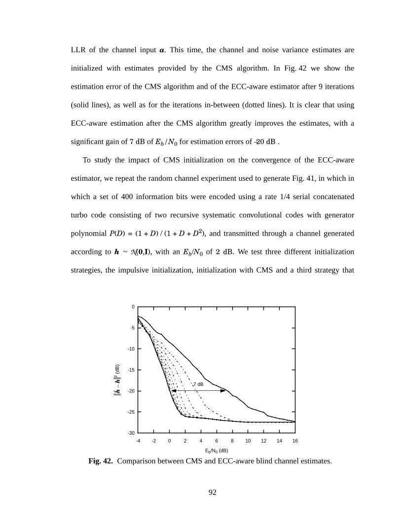
92

LLR of the channel input a. This time, the channel and noise variance estimates are

initialized with estimates provided by the CMS algorithm. In Fig. 42 we show the

estimation error of the CMS algorithm and of the ECC-aware estimator after 9 iterations

(solid lines), as well as for the iterations in-between (dotted lines). It is clear that using

ECC-aware estimation after the CMS algorithm greatly improves the estimates, with a

significant gain of 7 dB of Eb/N0 for estimation errors of –20 dB .

To study the impact of CMS initialization on the convergence of the ECC-aware

estimator, we repeat the random channel experiment used to generate Fig. 41, in which in

which a set of 400 information bits were encoded using a rate 1/4 serial concatenated

turbo code consisting of two recursive systematic convolutional codes with generator

polynomial P(D) = (1 + D) / (1 + D + D2), and transmitted through a channel generated

according to h ~ N(0,I), with an Eb/N0 of 2 dB. We test three different initialization

strategies, the impulsive initialization, initialization with CMS and a third strategy that

Fig. 42. Comparison between CMS and ECC-aware blind channel estimates.

-4 -2 0 2 4 6 8 10 12 14 16

-30

-25

-20

-15

-10

-5

0

Eb/N0 (dB)

2(d

B)

hh

– 7 dB

93

consistsof initializing the equalizeroutput to sign(rk), i.e., we make decisionson the

transmittedcodeword ignoring noise and ISI. In other words, at the first iteration the

channelis estimatedwith sign(rk) replacingtanh . The resulting WER for these

initialization strategies is shown in Fig. 43. As we can see, even though the CMS

algorithmcancertainlyhelptheconvergenceof theECC-awareestimatorat high SNR,it

is not very helpful at low SNR. This happensbecauseCMS operatesin the uncoded

domain,soin ourexampleit “sees”anSNRof –4 dB. In otherwords,in theregionwhere

theECC-awareestimatoris mostuseful,thelow SNRregion,CMS is not ableto produce

reliable channel estimates.

Lk2

-------

Fig. 43. WER for different initialization strategies.

0 5 10 15 20 25 300.08

1

Iteration

WE

R

CMS

Impulsive

Ignoring ISI

0.1

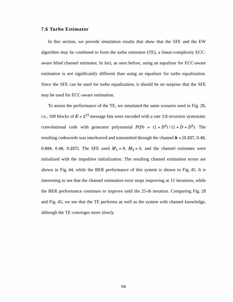
94

7.6 Turbo Estimator

In this section, we provide simulation results that show that the SFE and the EW

algorithm may be combined to form the turbo estimator (TE), a linear-complexity ECC-

aware blind channel estimator. In fact, as seen before, using an equalizer for ECC-aware

estimation is not significantly different than using an equalizer for turbo equalization.

Since the SFE can be used for turbo equalization, it should be no surprise that the SFE

may be used for ECC-aware estimation.

To assess the performance of the TE, we simulated the same scenario used in Fig. 28,

i.e., 100 blocks of K = 215 message bits were encoded with a rate 1/2 recursive systematic

convolutional code with generator polynomial P(D) = (1 + D2) / (1 + D + D2). The

resulting codewords was interleaved and transmitted through the channel h = [0.227, 0.46,

0.688, 0.46, 0.227]. The SFE used M1 = 9, M2 = 5, and the channel estimates were

initialized with the impulsive initialization. The resulting channel estimation errors are

shown in Fig. 44, while the BER performance of this system is shown in Fig. 45. It is

interesting to see that the channel estimation error stops improving at 15 iterations, while

the BER performance continues to improve until the 25-th iteration. Comparing Fig. 28

and Fig. 45, we see that the TE performs as well as the system with channel knowledge,

although the TE converges more slowly.

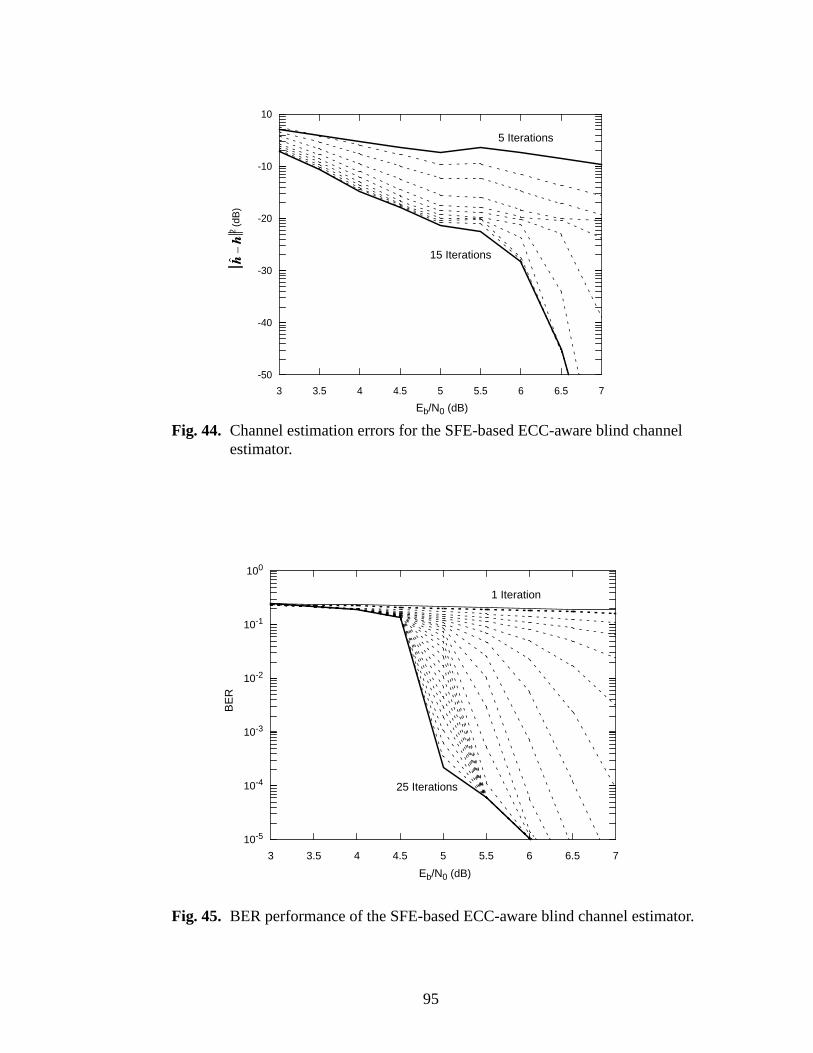
95

Fig. 44. Channel estimation errors for the SFE-based ECC-aware blind channelestimator.

3 3.5 4 4.5 5 5.5 6 6.5 7

-50

-40

-30

-20

-10

10

2 (d

B)

hh

–

Eb/N0 (dB)

5 Iterations

15 Iterations

Fig. 45. BER performance of the SFE-based ECC-aware blind channel estimator.

Eb/N0 (dB)

BE

R

3 3.5 4 4.5 5 5.5 6 6.5 7

10-5

10-4

10-3

10-2

10-1

100

1 Iteration

25 Iterations

96

7.7 Summary

In this chapter, we proposed an ECC-aware blind channel estimator, an iterative

channel estimator that benefits from the presence of coding. We provided examples of the

good quality of ECC-aware estimates. For instance, we showed that a turbo equalizer

using ECC-aware estimates may perform almost as well as a turbo equalizer with channel

knowledge. We also compared ECC-aware estimates to ECC-ignorant estimates, and

showed that a gain of as much as 7 dB is possible for an estimation error of -20 dB.

Furthermore, we showed that systems based on ECC-aware estimates may operate at very

low SNR, where ECC-ignorant estimates yield poor performance. Finally, we proposed

the turbo estimator, a linear-complexity ECC-aware channel estimator based on the EW

algorithm of chapter 4 and the SFE of chapter 5. We showed that the SFE-based ECC-

aware estimator retains all the desirable properties of the BCJR-based estimator.

97

CHAPTER 8

Conclusions

8.1 Summary of Contributions

In this work, we proposed and analyzed linear-complexity techniques for iterative

channel estimation and equalization. Because of the way these techniques are designed,

they may benefit from the presence of ECC, and hence may be used for turbo equalization

and ECC-aware channel estimation.

In chapter 2, the problem of blind channel estimation for a coded system is introduced.

A maximum-likelihood estimator is prohibitively complex, so this problem is normally

divided in three subproblems: channel estimation, equalization and decoding. We

discussed the divide and conquer approach, in which each of these subproblems is solved

independently. We also discussed turbo equalizers and the EM algorithm. These are

iterative algorithms that provide approximate solutions to otherwise intractable problems:

respectively, joint decoding and equalization for known channels, and joint estimation and

equalization for uncoded systems.

Turbo equalizers and the EM algorithm provide better performance than their non-

iterative counterparts. Combining them into an iterative receiver that provides channel

estimates that benefit from the presence of ECC is almost straightforward. However, these

techniques suffer from complexity and convergence problems. The goal of this thesis was

98

to propose a system whose per-symbol computational complexity grows linearly with the

number of coefficients in the system. The proposed system is less prone to

misconvergence than systems based on the EM algorithm.

In chapter 3, we proposed the SEM algorithm, a linear complexity channel estimator

[20] that performs almost as well as the EM algorithm, whose channel estimator has

quadratic complexity. More importantly, the SEM is not intrinsically tied to an equalizer,

so further complexity reduction is possible if the BCJR equalizer in the EM algorithm is

replaced by a lower-complexity equalizer. We presented a detailed analysis of the SEM

algorithm for a scalar channel, and compared the performance of the SEM and the EM

algorithm for channels that introduce ISI. Simulations established that the performance is

not significantly degraded with the SEM algorithm.

In chapter 4, we studied the convergence issues of the EM algorithm. We showed that

in some cases of misconvergence of the EM algorithm, the resulting channel estimates

may be seen as shifted versions of the actual channel. With this observation in mind, we

developed the EW algorithm, a linear complexity channel estimator with better

convergence properties than the EM algorithm [20].

In chapter 5, we addressed the complexity of the BCJR equalizer, which is used in the

EM algorithm and in turbo equalizers. We discussed techniques that replace the BCJR

equalizer by a linear equalizer and an ISI canceller. The output of the linear equalizer

contains residual ISI, which is removed by the ISI canceller using the extrinsic

information at the equalizer output. Most of the techniques proposed in the literature have

99

quadratic complexity. Some linear-complexity techniques have also been proposed. We

proposed the SFE, a linear-complexity soft-output equalizer that is suited for iterative

applications [52] and that outperforms existing linear-complexity equalizers.

In chapter 6, we studied the application of the SFE in turbo equalization. We discussed

some issues arising in this application, and we showed that the SFE outperforms other

linear-complexity equalizers in this context. We also discussed EXIT charts, and showed

the charts of various equalizers.

Finally, in chapter 7, we proposed the turbo estimator (TE), an ECC-aware channel

estimator that uses the fact that the transmitted sequence was encoded to improve blind

and semi-blind channel estimates. These ECC-aware channel estimators may be seen as a

combination of the EM or EW algorithm with a turbo equalizer. Therefore, using the SFE

for equalization we obtain a linear-complexity ECC-aware estimator [17]. We showed that

ECC-aware blind estimates may yield a BER performance similar to that of systems with

channel knowledge. We also showed that ECC-aware blind estimates allow systems to

operate at an SNR so low that other ECC-ignorant blind estimators fail. Because of these

observations, ECC-aware blind estimators may be essential for blind systems to enjoy the

full benefits of turbo equalization.

100

8.2 Directions for Future Research

Even though the EW algorithm improves the convergence of the iterative channel

estimator, there is still a nonzero probability that the estimator will not converge to the

correct channel estimates. A better understanding of the reasons for misconvergence is

needed, and a globally convergent blind iterative channel estimator is yet to be

determined.

The performance of iterative schemes is hard to determine, which has motivated the

development of approximate analysis tools such as the EXIT charts. However, most of

these tools are based on simulations. A purely theoretical tool would be of interest.

When comparing the SFE to a DFE, we have observed that sometimes hard feedback

gives better performance than soft feedback, and sometimes the reverse happens. A deeper

investigation of this behavior should be conducted. For instance, one could try to

determine in which cases hard information works better than soft information, and in

which cases the reverse happens.

The techniques proposed in this research were tested on general simulation channels.

It would be interesting to test them in real world applications. One possibility that is

currently under investigation in the Communication Theory Research Group at the

Georgia Institute of Technology is the use of the SFE for equalization in magnetic

recording channels. In magnetic recording systems, the received signal is normally filtered

with a linear equalizer so that the cascade of the channel and the equalizer has a given

impulse response. Normally, this impulse response is short enough that a BCJR equalizer

may be used. However, as the recording density increases, so does the length of the

impulse response of the cascade of the channel and the equalizer. Furthermore, the linear

101

equalizer introduces some noise enhancement and does not benefit from turbo

equalization. The system under investigation would replace the linear equalizer and the

BCJR equalizer by a single SFE. It is expected that the SFE-base system may even

outperform the BCJR-based system, since the latter suffers from the noise enhancement

introduced by the linear equalizer.

Finally, it is a well-known fact that blind channel estimators cannot account for delays.

In other words, the sequence at the blind-equalizer output may be a delayed version of the

transmitted sequence. If a delayed sequence is fed to the deinterleaver, the resulting

sequence will be uncorrelated to the decoder output. In this work, this delay issue did not

arise since we assumed the channel length to be known. In practical applications, however,

this assumption is usually false. Therefore, a technique for resolving the delay must be

found.

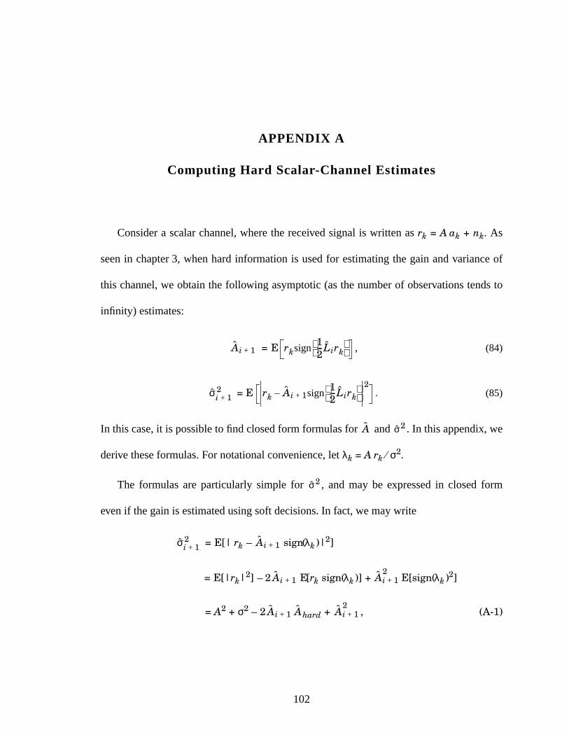
102

APPENDIX A

Computing Hard Scalar-Channel Estimates

Consider a scalar channel, where the received signal is written as rk = A ak + nk. As

seen in chapter 3, when hard information is used for estimating the gain and variance of

this channel, we obtain the following asymptotic (as the number of observations tends to

infinity) estimates:

= E , (84)

= E . (85)

In this case, it is possible to find closed form formulas for and . In this appendix, we

derive these formulas. For notational convenience, let λk = A rk ⁄σ2.

The formulas are particularly simple for , and may be expressed in closed form

even if the gain is estimated using soft decisions. In fact, we may write

= E[| rk – sign(λk )|2]

= E[|rk|2] – 2 E[rk sign(λk )] + E[sign(λk )2]

= A2 + σ2 – 2 hard + , (A-1)

Ai 1+ rksign12--- Lirk

σi 1+2 rk Ai 1+ sign

12--- Lirk

–2

A σ2

σ2

σi 1+2 Ai 1+

Ai 1+ Ai 1+2

Ai 1+ A Ai 1+2

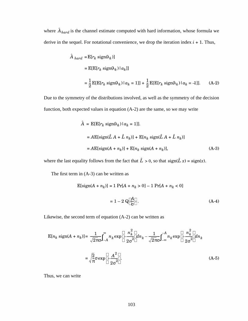
103

where hard is the channel estimate computed with hard information, whose formula we

derive in the sequel. For notational convenience, we drop the iteration index i + 1. Thus,

hard =E[rk sign(λk )]

= E[E[rk sign(λk )|ak]]

= E[E[rk sign(λk )|ak = 1]] + E[E[rk sign(λk )|ak = –1]]. (A-2)

Due to the symmetry of the distributions involved, as well as the symmetry of the decision

function, both expected values in equation (A-2) are the same, so we may write

= E[E[rk sign(λk )|ak = 1]].

= AE[sign( A + nk)] + E[nk sign( A + nk)]

= AE[sign(A + nk)] + E[nk sign(A + nk)], (A-3)

where the last equality follows from the fact that > 0, so that sign( x) = sign(x).

The first term in (A-3) can be written as

E[sign(A + nk)] = 1 Pr[A + nk > 0] – 1 Pr[A + nk < 0]

= 1 – 2 Q . (A-4)

Likewise, the second term of equation (A-2) can be written as

E[nk sign(A + nk)]=

= . (A-5)

Thus, we can write

A

A

12--- 1

2---

A

L L L L

L L

Aσ----

12πσ

--------------- nknk

2

2σ2----------–

nkdexpA–

∞∫ 1

2πσ--------------- nk

nk2

2σ2----------–

nkdexp∞–

A–

∫–

2π---σ A2

2σ2----------–

exp

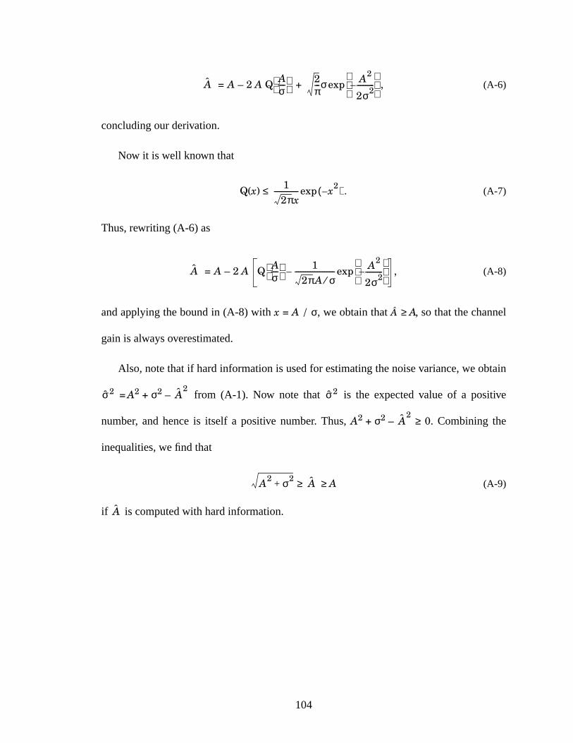
104

= A – 2 A Q + , (A-6)

concluding our derivation.

Now it is well known that

Q(x) ≤ . (A-7)

Thus, rewriting (A-6) as

= A – 2 A , (A-8)

and applying the bound in (A-8) with x = A / σ, we obtain that  ≥ A, so that the channel

gain is always overestimated.

Also, note that if hard information is used for estimating the noise variance, we obtain

= A2 + σ2 – from (A-1). Now note that is the expected value of a positive

number, and hence is itself a positive number. Thus, A2 + σ2 – ≥ 0. Combining the

inequalities, we find that

≥ ≥ A (A-9)

if is computed with hard information.

A Aσ----

2π---σ A2

2σ2----------–

exp

12πx

-------------- x2–( )exp

A Q Aσ----

12π A σ⁄

----------------------- A2

2σ2----------–

exp–

σ2 A2

σ2

A2

A2 σ2+ A

A

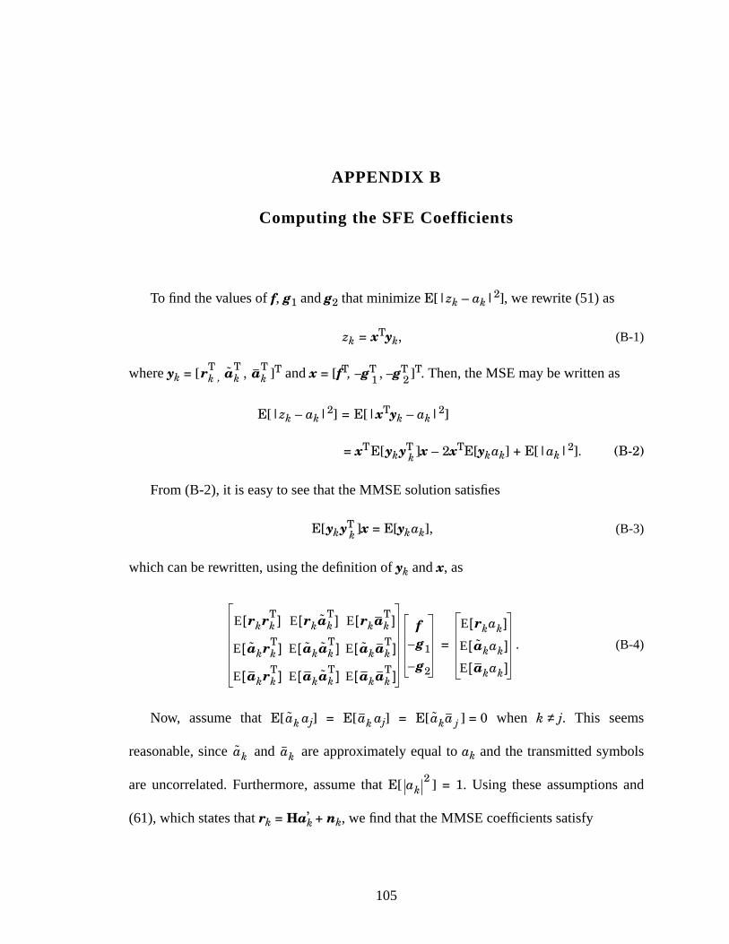
105

APPENDIX B

Computing the SFE Coefficients

To find the values of f, g1 and g2 that minimize E[|zk – ak|2], we rewrite (51) as

zk = xTyk, (B-1)

where yk = [ , , ]T and x = [fT, – gT1 , – gT

2 ]T. Then, the MSE may be written as

E[|zk – ak|2] = E[|xTyk – ak|2]

= xTE[ykyTk ]x – 2xTE[ykak] + E[|ak|2]. (B-2)

From (B-2), it is easy to see that the MMSE solution satisfies

E[ykyTk ]x = E[ykak], (B-3)

which can be rewritten, using the definition of yk and x, as

= . (B-4)

Now, assume that E[ aj] = E[ aj] = E[ ] = 0 when k ≠ j. This seems

reasonable, since and are approximately equal to ak and the transmitted symbols

are uncorrelated. Furthermore, assume that E[ ] = 1. Using these assumptions and

(61), which states that rk = Ha’k + nk, we find that the MMSE coefficients satisfy

rkT ak

T akT

E rkrkT[ ] E rkak

T[ ] E rkakT[ ]

E akrkT[ ] E akak

T[ ] E akakT[ ]

E akrkT[ ] E akak

T[ ] E akakT[ ]

fg1–

g2–

E rkak[ ]

E akak[ ]

E akak[ ]

ak ak aka j

ak ak

ak2

106

= , (B-5)

where E1 = E[| |2], E2 = E[| |2], α1 = E[ ak], and α2 = E[ ak]. The vector h0 is

the 0-th column of H, where the columns of H are numbered as H = [ , …, ].

Also, H1 = [ , … h–1 ] and H2 = [h1, … ].

The last two block-rows in (B-5) yield

g1 = (α1 ⁄E1) H1Tf (B-6)

g2 = (α2 ⁄E2) H2Tf . (B-7)

Using these values, the first row of (B-5) may be written as

(HHT+ σ2I – H1H1T – H2H2

T )f = h0, (B-8)

yielding

f = (HHT – H1H1T – H2H2

T + σ2I)–1 h0, (B-9)

which completes the derivation of the SFE coefficients.

Finally, assume that zk = Aak + vk, where A is a gain and vk an equivalent noise with

variance , assumed to be Gaussian and independent of ak. In this case, A = E[zkak].

Using (B-1), this yields A = xTE[ykak]. However, as seen in (B-5), E[ykak] =

[ , 0T, 0T]T. Thus, since x = [fT, – gT1 , – gT

2 ]T, we have that

A = fTh0. (B-10)

HHT σ2I+ α1H1 α2H2

α1H1T E1I 0

α2H2T 0 E2I

fg1–

g2–

h0

00

ak ak ak ak

h M1– hM2 µ+

h M1– hM2 µ+

α12

E1-------

α22

E2-------

α12

E1-------

α22

E2-------

σv2

h0T

107

Furthermore, E[ ] = A2 + . However, using (B-1), we may write E[ ] =

xTE[ykyTk ]x. Then, using (B-3), we get that E[ ] = xTE[ykak] = A. Thus,

= A – A 2. (B-11)

zk2 σv

2 zk2

zk2

σv2

108

References

[1] E. A. Lee andD. G. Messerschmitt,Digital Communication, SecondEdition,

Kluwer Academic Publishers, 1994.

[2] S. B. Wicker, Error Control Systemsfor Digital CommunicationandStorage,

Prentice-Hall, 1995.

[3] C. P. Williams and S. H. Clearwater, Explorations in QuantumComput-

ing,Spinger-Verlag, New York, 1998.

[4] Poor, H. V., An Introductionto SignalDetectionandEstimation, SecondEdi-

tion, Springer-Verlag, 1994.

[5] L. Ljung andT. Söderström,Theoryand practiceof recursive identification,

MIT Press, Cambridge, Mass., 1983.

[6] J.Ayadi,E. deCarvalhoandD. T. M. Slock,“Blind andSemi-BlindMaximum

LikelihoodMethodsfor FIR MultichannelIdentification,” IEEE ICASSP, vol.

6, pp. 3185 -3188, 1998.

[7] S. Haykin, ed,Blind Deconvolution, Prentice-Hall, 1994.

[8] Z. Ding andY. Li, Blind equalizationand identification, MarcelDekker, New

York, 2001.

109

[9] C. Berrou,A. GlavieuxandP. Thitimajshima,“NearShannonLimit Error-Cor-

rectingCodingandDecoding,” IEEE International Conference on Commun.,

pp. 1064-1070, May 1993.

[10] D. J.MacKay, “GoodErrorCorrectingCodesBasedonVerySparseMatrices,”

IEEE T. Info. Theory, p. 399-431, May 1999.

[11] S.Benedetto,D. Divsalar, G. MontorsiandF. Pollara,“SerialConcatenationof

Interleaved Codes:PerformanceAnalysis, Design and Iterative Decoding,”

IEEE Trans. Information Theory, vol. 44, no. 3, pp. 909-926, May 1998.

[12] J.Garcia-FriasandJ.D. Villasenor, “Blind TurboDecodingandEqualization,”

IEEE Vehicular Technology Conference, pp. 1881-1885, v. 3, May 1999.

[13] J.Garcia-FriasandJ.D. Villasenor, “CombinedBlind EqualizationandTurbo

Decoding,” IEEE Communications Theory Mini-Conference, pp. 52-57,June

1999.

[14] K. -D. Kammeyer, V. Kühn andT. Peterman,“Blind andNonblindTurboEsti-

mation for FastFadingGSM Channels,” IEEE Journal on Selected Areas in

Communications, vol. 19, no. 9, pp. 1718-1728, Sep. 2001.

[15] A. O. Berthet,B. S.ÜnalandR. Visoz,“IterativeDecodingof Convolutionally

EncodedSignalsover Multipath RayleighFadingChannels,” IEEE Journal on

Selected Areas in Communications, vol. 19, no. 9, pp. 1728-1743, Sep. 2001.

[16] P. Ha andB. Honary, “ImprovedBlind Detector,” IEEE Vehicular Technology

Conference, pp. 1196-1199, v. 2, May 2000.

110

[17] R. Lopesand J. Barry, “Exploiting Error-Control Coding in Blind Channel

Estimation,” IEEE Global Communications Conference, vol. 2, pp.1317-1321,

San Antonio, TX, November 2001.

[18] C. Douillard, M. Jezequel,C. Berrou,A. Picart,P. Didier and A. Glavieux,

“Iterative Correctionof IntersymbolInterference:Turbo Equalization,” Euro-

pean Transaction on Telecommunications, vol. 6, no.5, pp 507-511,Sep.-Oct.

1995.

[19] D. RaphaeliandY. Zarai, “CombinedTurbo EqualizationandTurbo Decod-

ing,” IEEE Communications Letters, vol. 2, no.4, pp.107-109, April 1998.

[20] R. R. LopesandJ.R. Barry, “Blind Iterative ChannelIdentificationandEqual-

ization,” IEEE International Conference on Communications, pp. 2256-2260,

Finland, June 2001.

[21] M. FederandJ. A. Catipovic, “Algorithms for Joint ChannelEstimationand

Data Recovery— Application to Equalization in Underwater Communica-

tions,” IEEE J. Oceanic Eng., vol. 16, no. 1, pp. 42–5, Jan. 1991.

[22] G. K. KalehandR. Vallet, “Joint ParameterEstimationandSymbolDetection

for Linear or NonlinearUnknown Channels”,IEEE Transactions on Commu-

nications, vol. 42, no. 7, pp. 2406-2413, July 1994.

[23] C. Anton-Haro,J.A. R. FonollosaandJ.R. Fonollosa,“Blind ChannelEstima-

tion and Data DetectionUsing Hidden Markov Models,” IEEE Trans. Sig.

Proc., vol. 45, no. 1, pp. 241-246, Jan 1997.

111

[24] V. Krishnamurthy, J. B. Moore, “On-Line Estimation of Hidden Markov Model

Parameters Based on the Kullback-Leibler Information Measure,” EEE Trans.

Sig. Proc., vol. 41, no. 8, pp. 2557-2573, Aug 1993.

[25] L. B. White, S. Perreau, P. Duhamel, “Reduced Complexity Blind Equalization

for FIR Channel Input Markov Models”, IEEE International Conference on

Communications, vol. 2, pp.993-997, 1995.

[26] M. Shao and C. L. Nikias, “An ML/MMSE Estimation Approach to Blind

Equalization”, ICASSP, vol. 4, pp. 569-572, 1994.

[27] H. A. Cirpan and M. K. Tsatsanis, “Stochastic Maximum Likelihood Methods

for Semi-Blind Channel Equalization,” Signal Processing Letters, vol. 5, no. 1,

pp. 1629-1632, Jan 1998.

[28] B. P. Paris, “Self-Adaptive Maximum-Likelihood Sequence Estimation,” IEEE

Global Telecommunications Conf., vol. 4, pp. 92-96, 1993.

[29] L. R. Bahl, J. Cocke, F. Jelinek, and J. Raviv, “Optimal Decoding of Linear

Codes for Minimizing Symbol Error Rate,” IEEE Transactions on Information

Theory, pp. 284-287, March 1974.

[30] A. Glavieux, C. Laot and J. Labat, “Turbo Equalization Over a Frequency

Selective Channel,” International Symp. on Turbo Codes and Related Topics,

Brest, France, pp. 96-102, Sep 1997.

[31] Z. Wu and J. Cioffi, “Turbo Decision Aided Equalization for Magnetic Record-

ing Channels,” IEEE Global Communications Conference, pp. 733-738, Dec.

1999.

112

[32] D. Raphaeliand A. Saguy, “ReducedComplexity APP for Turbo Equaliza-

tion,” IEEE International Conf. Comm., vol. 3, pp. 1940-1943, 2002.

[33] A. DejongheandL. Vanderdorpe,“TurboEqualizationfor Multilevel Modula-

tion: an Efficient Low-Complexity Scheme,” IEEE International Conference

on Communications, vol. 3, pp. 1863-1867, 2002.

[34] J. Rößler, W. Gerstacker, A. Lampe, and J. Huber, “Matched-Filter- and

MMSE-BasedIterative Equalizationwith Soft Feedbackfor QPSKTransmis-

sion,” International Zurich Seminar on Broadband Comm., pp. 19-1 - 19-6,

February 2002.

[35] M. Tüchler, R. KoetterandA. C. Singer, “Turbo Equalization:Principlesand

New Results,” IEEE Transactions on Communications, vol. 50,no.5, pp.754-

767, May 2002.

[36] A. Berthet,R. VisozandP. Tortelier, “Sub-OptimalTurbo-Detectionfor Coded

8-PSKSignalsover ISI Channelswith Applicationto EDGEAdvancedMobile

Systems,” IEEE International Symp. on Personal, Indoor and Mobile Radio

Comm., pp. 151-157, Sep. 2000.

[37] R. Visoz, A. O. Berthett and J. J. Boutros, “Reduced-Complexity Iterative

Decodingand ChannelEstimationfor SpaceTime BICM over Frequency-

Selective Wireless Channels,” IEEE Symposion on Personal, Indoor and

Mobile Radio Communications, vol. 3, pp. 1017 -1022, 2002.

[38] C. Fragouli,N. Al-Dhahir andW. Turin, “PrefilteredM-BCJREqualizationof

Space-Time-CodedTransmissionover Frequency-Selective Channels,” Conf.

Info. Sciences and Systems, pp. 841-845, March 2001.

113

[39] A. A. Chang and G. Wornell, “A Class of Block-Iterative Equalizersfor

IntersymbolInterferenceCancellation:Fixed ChannelsResults,” IEEE Trans.

on Comm., vol. 49, no. 11, pp. 1966-1976, Nov. 2001.

[40] A. P. Dempster, N. M. Laird and D. B. Rubin, “Maximum Likelihood from

IncompleteDataVia theEM Algorithm”, Journal of the Royal Statistics Soci-

ety, vol. 39, no. 1, pp 1-38, 1997.

[41] L. E. Baum et al. “A Maximization TechniqueOccurring in the Statistical

Analysisof ProbabilisticFunctionsof Markov Chains”,Annals of Mathemat-

ics Statistics, vol. 41, pp. 164-171, 1970.

[42] W. Ryan,“A Turbo CodeTutorial,” unpublished,http://www.ece.arizona.edu/

~ryan/turbo2c.pdf

[43] G. Stüber, Principles of Mobile Communication, Kluwer AcademicPublishers,

2nd Edition, 2001.

[44] J. A. C. Bingham,‘‘Multicarrier Modulationfor DataTransmission:An Idea

whoseTime hasCome,’’ IEEE Communications Magazine, May 1990,pp. 5-

14.

[45] S. tenBrink, “ConvergenceBehavior of Iteratively DecodedParallelConcate-

nated Codes,” IEEE Trans. on Comm., vol. 40, pp. 1727-1737, Oct. 2001.

[46] R. G. Gallager, Information Theory and Reliable Communication, Wiley, 1968.

[47] H.-A. Loeliger and D. Arnold, “On the Information Rate of Binary-Input

Channels with Memory,” IEEE Int. Symp. Inform. Theory, p. 164, July 2002.

[48] J. Proakis,Digital Communications, McGraw-Hill, 1995.

114

[49] http://spib.rice.edu/spib/data/signals/comm/microwave/chan14a

[50] K. R. Narayanan, X. Wang and G. Yue, “LDPC code design for turbo equaliza-

tion,” IEEE Information Theory Workshop, pp 57 -60, 2002.

[51] Z. Ding and J. Liang, “A Cumulant Matrix Subspace Algorithm for Blind Sin-

gle FIR Identification,” IEEE Transactions on Signal Processing, vol. 49, no. 2,

pp. 325-333, Feb 2001.

[52] R. Lopes and J. Barry, “Soft-Output Decision-Feedback Equalizer with Priors,”

IEEE Global Communications Conference, 2003.

115

VITA

RenatoLopesis from Campinas,Brazil. He receivedBachelor’s andMaster’s degrees

from theStateUniversityof Campinas(UNICAMP) in 1995and1997,respectively, both

in ElectricalEngineering.In 1993he worked with the TelephoneCompany of Tampere,

Finland, in the areaof GSM services.In 1994 he worked with PROMON Eletrônica,

Campinas,Brazil, in thedepartmentresponsiblefor testingswitchboards.He receivedthe

Ph.D.degreefrom theGeorgia Instituteof Technologyin 2003.During his Ph.D.,hewas

supportedby CAPES, and was also a teachingand researchassistantat the Georgia

Instituteof Technology. He will join UNICAMP asa post-doctoratefellow. His research

interestarein thegeneralareaof communicationstheory, with emphasisin equalization,

channel estimation and iterative techniques for communications.