Iterative and adjusting method for computing stream function and velocity potential in limited...

Appl. Math. Mech. -Engl. Ed., 33(6), 687–700 (2012)DOI 10.1007/s10483-012-1580-9c©Shanghai University and Springer-Verlag

Berlin Heidelberg 2012

Applied Mathematicsand Mechanics(English Edition)

Iterative and adjusting method for computing stream function andvelocity potential in limited domains and convergence analysis∗

Ai-bing LI (��), Li-feng ZHANG (��), Zeng-liang ZANG (��),Yun ZHANG (� �)

(Institute of Meteorology, PLA University of Science and Technology,

Nanjing 211101, P. R. China)

Abstract The stream function and the velocity potential can be easily computed by

solving the Poisson equations in a unique way for the global domain. Because of the var-

ious assumptions for handling the boundary conditions, the solution is not unique when

a limited domain is concerned. Therefore, it is very important to reduce or eliminate the

effects caused by the uncertain boundary condition. In this paper, an iterative and ad-

justing method based on the Endlich iteration method is presented to compute the stream

function and the velocity potential in limited domains. This method does not need an

explicitly specifying boundary condition when used to obtain the effective solution, and

it is proved to be successful in decomposing and reconstructing the horizontal wind field

with very small errors. The convergence of the method depends on the relative value for

the distances of grids in two different directions and the value of the adjusting factor. It is

shown that applying the method in Arakawa grids and irregular domains can obtain the

accurate vorticity and divergence and accurately decompose and reconstruct the original

wind field. Hence, the iterative and adjusting method is accurate and reliable.

Key words limited domain, stream function, velocity potential, iteration and adjust-

ment, convergence

Chinese Library Classification O302, P425

2010 Mathematics Subject Classification 65N12, 76M20, 86-08

1 Introduction

The stream function and the velocity potential, which are widely used in meteorology, aretwo important physical quantities in describing the non-divergent and irrotational motion ofwind fields. They are useful in the wind field decomposition[1]. They can reflect the vorticityand divergence[2], and they are crucial variables in the atmospheric circulation analysis anddata assimilation research[3–6].

The stream function and the velocity potential, which are mainly derived by solving thePoisson equations, are not directly observed variables. The stream function and the velocitypotential from the vorticity and divergence or the wind field can be easily computated in the

∗ Received Sept. 26, 2011 / Revised Mar. 1, 2012Project supported by the National Natural Science Foundation of China (No. 40975031)Corresponding author Li-feng ZHANG, Professor, Ph.D., E-mail: [email protected]

688 Ai-bing LI, Li-feng ZHANG, Zeng-liang ZANG, and Yun ZHANG

global domain for the periodic boundary condition and have unique solutions[7]. However,because of the uncertain and various assumptions on the boundary conditions, the solutionis not unique when the method is used in a limited domain[8]. Meanwhile, the calculativeerrors cannot be ignored. To get over the difficulty in handling boundary conditions in limiteddomains, several methods have been proposed.

Tangri[9] assumed the boundary of the stream function with the zero value to compute thestream function in a limited area. Phillips[10] used the difference between the observed valueof the normal velocity at every point and its mean value for all points along the boundary tocompute the boundary value of the stream function. This method is not satisfactory and cancause large errors between the original and reconstructed wind fields as shown by Hawkins andRosenthal[1]. Brown and Neilon[11] improved the method in a modified form and directly usedthe observed value of the wind field at every point on the boundary.

The methods mentioned above compute the stream function and the velocity potential sep-arately by solving the single Poisson equation. In fact, the stream function and the velocitypotential are closely related, and they can be computed at the same time. Thus, Sangster[12]

proposed the following method. First, compute the velocity potential with the zero value ofthe boundary, and obtain the divergent wind field by calculating the partial derivative. Then,solve the stream function with its boundary value that is determined by the difference betweenthe observed and divergent wind fields. However, this method is inaccurate to decompose andreconstruct the horizontal wind field in limited domains[13]. Based on Sangster’s method, aniterative method was introduced by Shukla and Saha[14] by constantly updating the values ofthe stream function and the velocity potential on the boundary. Bijlsma et al.[8] separatedthe stream function and the velocity potential into two parts and designed another iterativemethod. Lynch[15–16] discussed the iterative and computational problems for solving the streamfunction and the velocity potential on various boundary conditions. He found that, though therewere some improvements in the results using Bijlsma’s method, the two iterations were bothnon-convergent. Chen and Kuo[17–18] proposed a method of theharmonic-sine/cosine series ex-pansion which could accurately obtain the reconstructed wind field. However, the externalparts of the stream function and the velocity potential are also determined by the boundary.Also, they proved that the solution of the stream function and the velocity potential in limiteddomains was not unique, but the sum of the rotational and divergent wind fields decomposedfrom the original wind field should be unique. Thus, a criterion for computing the stream func-tion and the velocity potential in limited domains was defined to see whether the reconstructedwind field was consistent with the original wind field. Recently, Zhu and Zhu[19], Zhu et al.[20],Zhou et al.[21], and Zhou and Cao[22] have done some studies on how to eliminate the effectscaused by the limited boundary when computing the stream function and the velocity potentialor decomposing the wind field into two different parts.

Except by solving the Poisson equations to decompose the wind field, some methods fromother angles have been proposed. Endlich[23] obtained the rotational wind field using twoadjustments at every iteration. However, he did not analyze the convergence of the method.By the variational principle, the stream function similar to the pressure field in some specificcases was obtained by Davies-Jones[24]. The method proposed by Li and Chao[25] is to computethe stream function and the velocity potential from the given horizontal wind field by solvinga minimization problem.

All the methods mentioned above are based on various assumptions for handling boundaryconditions. The uncertain boundary condition is the main difficulty for all calculations. There-fore, it is valuable to design a method which does not need explicit boundary conditions, butcan accurately compute the stream function and the velocity potential with small errors in thereconstructed wind field. In this paper, based on the Endlich iteration method, a new iterativeand adjusting method, which does not need a reasonable boundary condition, is proposed tocompute the stream function and the velocity potential in limited domains. This method can

Iterative and adjusting method for computing stream function and velocity potential 689

obtain the accurate result satisfying that the reconstructed wind field is consistent with theoriginal wind field. As the method is an iterative arithmetic, the convergence is also analyzedin this paper. Subsequently, this method is applied in different grids and irregular domains forverifying the accuracy and trustiness.

The outline of this paper is as follows. Section 2 reviews the Endlich iteration methodand introduces the iterative and adjusting method for computing the stream function and thevelocity potential. In Section 3, the convergence of the method is analyzed. Computationalexamples are presented to test the method in Section 4. Section 5 is the conclusions.

2 Iterative and adjusting method

2.1 Endlich iteration method for decomposing wind fieldThe horizontal wind field V can be separated into non-divergent and irrotational components

as follows[17–18,21]:V = Vψ + Vχ, (1)

where Vψ and Vχ are called the rotational wind field for the non-divergent motion and thedivergent wind field for the irrotational motion, respectively, which are defined by

Vψ = k ×∇ψ, Vχ = ∇χ. (2)

Here, ψ is the stream function, χ is the velocity potential, and k is a unit vector parallel to thelocal vertical direction. Given ψ and χ, V can be decomposed into Vψ and Vχ by (2).

From (1) and (2), the linear partial differential relationships between the stream function,the velocity potential, and the horizontal wind field can be described as

⎧⎪⎪⎨

⎪⎪⎩

u = uψ + uχ =∂χ

∂x− ∂ψ

∂y,

v = vψ + vχ =∂ψ

∂x+∂χ

∂y,

(3)

where (u, v), (uψ, vψ), and (uχ, vχ) represent the components of V , Vψ, and Vχ in the x-and y-directions. Hence, if the stream function and the velocity potential are computed, theoriginal wind field can be reconstructed by (3). The sum of the rotational and divergent windfields computed through the stream function and the velocity potential is the reconstructedwind field.

Using (2), the vertical component of the curl and the divergence of (1) can be, respectively,expressed as

⎧⎪⎪⎨

⎪⎪⎩

∇2ψ = ∇× V = ζ =∂vψ∂x

− ∂uψ∂y

,

∇2χ = ∇ · V = D =∂uχ∂x

+∂vχ∂y

.

(4)

Here, ζ is the vertical component of the relative vorticity, and D is the divergence.It is easy to find that Vψ and Vχ have linear partial differential relationships with ζ and D

in (4). (uψ, vψ) describes the non-divergent motion of atmosphere, for which the divergenceshould be zero, and the vorticity is equal to ζ computed from the original horizontal wind field.Hence, (uψ, vψ) satisfies the following equations:

⎧⎪⎪⎨

⎪⎪⎩

∂uψ∂x

+∂vψ∂y

= 0,

∂vψ∂x

− ∂uψ∂y

= ζ.

(5)


Based on (5), an iterative method, which successfully decomposed V into Vψ and Vχ using ζand D obtained from the observed wind field, was proposed by Endlich[23] in 1967. The Endlichiteration method for decomposing the horizontal wind field can be briefly stated as follows.

To begin with, a temporary wind field denoted by (ut, vt) with a random value is introduced,which usually does not satisfy (5). Here, the superscript t represents the temporary value ofthe computation at the latest stage of the iteration. The corresponding temporary divergenceand vorticity of (ut, vt) are denoted by Dt and ζt, respectively.

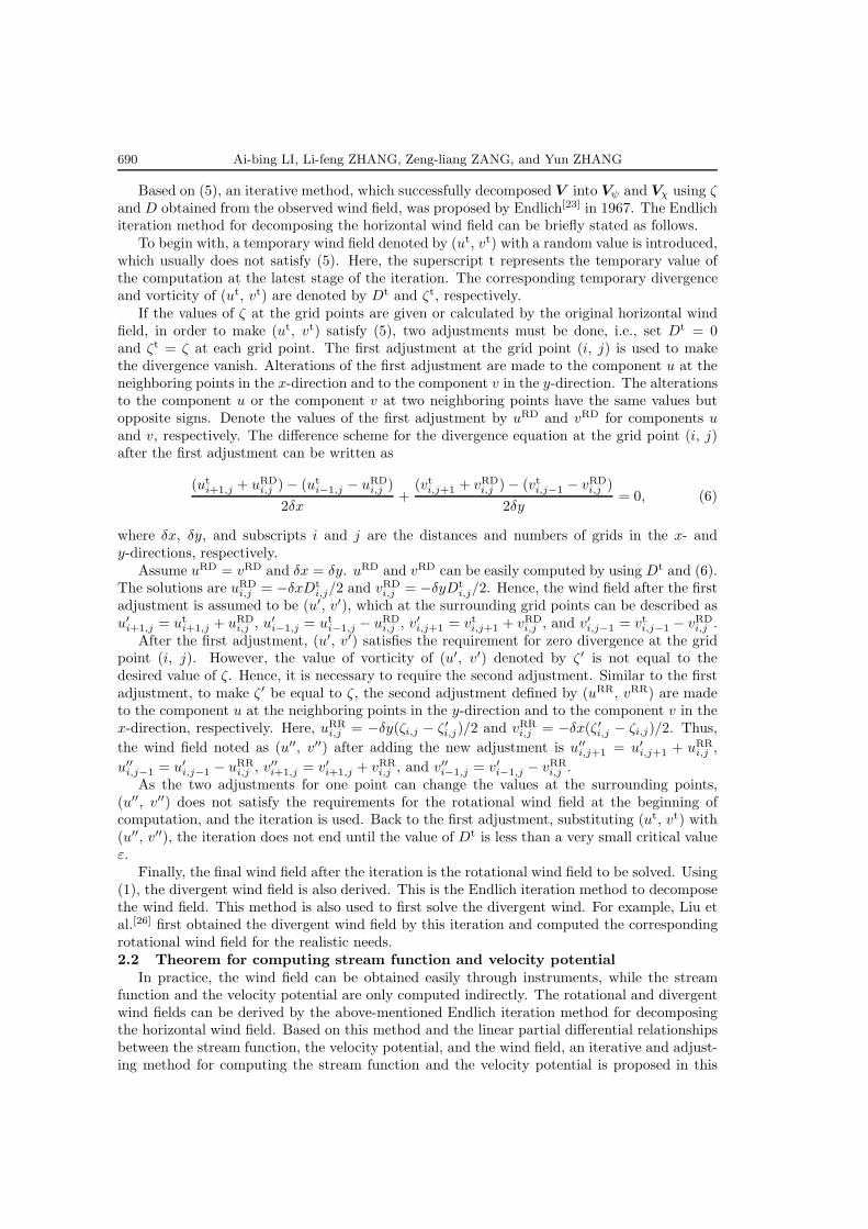
If the values of ζ at the grid points are given or calculated by the original horizontal windfield, in order to make (ut, vt) satisfy (5), two adjustments must be done, i.e., set Dt = 0and ζt = ζ at each grid point. The first adjustment at the grid point (i, j) is used to makethe divergence vanish. Alterations of the first adjustment are made to the component u at theneighboring points in the x-direction and to the component v in the y-direction. The alterationsto the component u or the component v at two neighboring points have the same values butopposite signs. Denote the values of the first adjustment by uRD and vRD for components uand v, respectively. The difference scheme for the divergence equation at the grid point (i, j)after the first adjustment can be written as

(uti+1,j + uRD

i,j ) − (uti−1,j − uRD

i,j )2δx

+(vti,j+1 + vRD

i,j ) − (vti,j−1 − vRD

i,j )2δy

= 0, (6)

where δx, δy, and subscripts i and j are the distances and numbers of grids in the x- andy-directions, respectively.

Assume uRD = vRD and δx = δy. uRD and vRD can be easily computed by using Dt and (6).The solutions are uRD

i,j = −δxDti,j/2 and vRD

i,j = −δyDti,j/2. Hence, the wind field after the first

adjustment is assumed to be (u′, v′), which at the surrounding grid points can be described asu′i+1,j = ut

i+1,j + uRDi,j , u′i−1,j = ut

i−1,j − uRDi,j , v′i,j+1 = vt

i,j+1 + vRDi,j , and v′i,j−1 = vt

i,j−1 − vRDi,j .

After the first adjustment, (u′, v′) satisfies the requirement for zero divergence at the gridpoint (i, j). However, the value of vorticity of (u′, v′) denoted by ζ′ is not equal to thedesired value of ζ. Hence, it is necessary to require the second adjustment. Similar to the firstadjustment, to make ζ′ be equal to ζ, the second adjustment defined by (uRR, vRR) are madeto the component u at the neighboring points in the y-direction and to the component v in thex-direction, respectively. Here, uRR

i,j = −δy(ζi,j − ζ′i,j)/2 and vRRi,j = −δx(ζ′i,j − ζi,j)/2. Thus,

the wind field noted as (u′′, v′′) after adding the new adjustment is u′′i,j+1 = u′i,j+1 + uRRi,j ,

u′′i,j−1 = u′i,j−1 − uRRi,j , v′′i+1,j = v′i+1,j + vRR

i,j , and v′′i−1,j = v′i−1,j − vRRi,j .

As the two adjustments for one point can change the values at the surrounding points,(u′′, v′′) does not satisfy the requirements for the rotational wind field at the beginning ofcomputation, and the iteration is used. Back to the first adjustment, substituting (ut, vt) with(u′′, v′′), the iteration does not end until the value of Dt is less than a very small critical valueε.

Finally, the final wind field after the iteration is the rotational wind field to be solved. Using(1), the divergent wind field is also derived. This is the Endlich iteration method to decomposethe wind field. This method is also used to first solve the divergent wind. For example, Liu etal.[26] first obtained the divergent wind field by this iteration and computed the correspondingrotational wind field for the realistic needs.2.2 Theorem for computing stream function and velocity potential

In practice, the wind field can be obtained easily through instruments, while the streamfunction and the velocity potential are only computed indirectly. The rotational and divergentwind fields can be derived by the above-mentioned Endlich iteration method for decomposingthe horizontal wind field. Based on this method and the linear partial differential relationshipsbetween the stream function, the velocity potential, and the wind field, an iterative and adjust-ing method for computing the stream function and the velocity potential is proposed in this


section. For simplicity, a square grid is considered only in this section, that is, δx = δy. Themethod can be described as follows.

Step 1 Calculate the temporary wind field with the given or computed stream function andvelocity potential. Assume that ψn and χn are the stream function and the velocity potentialafter n iterations, respectively. Here, the superscript n is the number of iterations. Whenn = 0, the stream function and the velocity potential can be arbitrary constants such as thezero values for the whole computational domains. According to (3), the temporary wind fielddenoted by (unt, vnt) can be obtained by computing the partial differential fields of the givenstream function and velocity potential. Thus, the solution of (unt, vnt) can be described as

⎧⎪⎪⎨

⎪⎪⎩

∂χn

∂x− ∂ψn

∂y= unt,

∂ψn

∂x+∂χn

∂y= vnt.

(7)

The values of unt and vnt change along with the growth of n, and they will maintain the stablevalues in the end.

Step 2 Make adjustments for the stream function and the velocity potential by the differ-ence between the temporary wind field and the original wind field. To make ψn and χn satisfy(3), according to adjustments in (6), some adjustments are made to ψn and χn in (7). Thedifference scheme of (7) after adjustments at the grid point (i, j) can be expressed as

⎧⎪⎪⎪⎨

⎪⎪⎪⎩

(χni+1,j + χxi,j) − (χni−1,j − χxi,j)2δx

− (ψni,j+1 + ψyi,j) − (ψni,j−1 − ψyi,j)2δy

= ui,j ,

(χni,j+1 + χyi,j) − (χni,j−1 − χyi,j)2δy

+(ψni+1,j + ψxi,j) − (ψni−1,j − ψxi,j)

2δx= vi,j ,

(8)

where the superscripts x and y of ψ and χ represent that the adjustments are made to the x-and y-directions for the stream function and the velocity potential, respectively. Thus, ψxi,j , ψ

yi,j

and χxi,j , χyi,j are the adjustments of ψ and χ at the grid point (i, j) in the x- and y-directions,

respectively. Subtracting (7) from (8) to eliminate ψn and χn, the linear partial differentialequations about adjustments can be written as follows:

⎧⎪⎪⎪⎨

⎪⎪⎪⎩

χxi,jδx

− ψyi,jδy

= ui,j − unti,j,

χyi,jδy

+ψxi,jδx

= vi,j − vnti,j .

(9)

For simplicity and the iteration convergence (the analysis of convergence will be shown inthe next section), the adjustments of the stream function and the velocity potential at the gridpoint (i, j) in the x- and y-directions are assumed to be

⎧⎪⎪⎪⎪⎪⎨

⎪⎪⎪⎪⎪⎩

ψxi,j = 0.5δx(vi,j − vnti,j),

ψyi,j = −0.5δy(ui,j − unti,j),

χxi,j = 0.5δx(ui,j − unti,j),

χyi,j = 0.5δy(vi,j − vnti,j).

(10)

Therefore, after n + 1 iterations, the stream function and the velocity potential at the


surrounding grid point (i, j) can be shown as⎧⎪⎪⎪⎪⎪⎪⎨

⎪⎪⎪⎪⎪⎪⎩

ψn+1i+1,j = ψni+1,j + ψxi,j , χn+1

i+1,j = χni+1,j + χxi,j ,

ψn+1i−1,j = ψni−1,j − ψxi,j , χn+1

i−1,j = χni−1,j − χxi,j ,

ψn+1i,j+1 = ψni,j+1 + ψyi,j , χn+1

i,j+1 = χni,j+1 + χyi,j ,

ψn+1i,j−1 = ψni,j−1 − ψyi,j , χn+1

i,j−1 = χni,j−1 − χyi,j .

(11)

Step 3 Judge whether the iteration should be ended or not. After making iteration andadjustment at each grid point, by (7), the temporary wind field denoted by (u(n+1)t, v(n+1)t) canbe obtained through the results of n+1 iterations. Also, the reconstructed horizontal wind fieldcan be computed through the given stream function and velocity potential. When adjustmentsare made at one grid point, the partial differential relationships between the stream function, thevelocity potential, and the wind field are destroyed at the surrounding grid points. Therefore,iterations must satisfy (3) at each grid point in limited domains. For the reconstructed wind fieldclose to the original wind field, a very small parameter ε (the value of ε may be 10−12 or evensmaller) is assigned as the critical value to end the iteration. When |u(n+1)t−u|+ |v(n+1)t−v| <ε, i.e., the absolute error between (u(n+1)t, v(n+1)t) and (u, v) is very smaller than the valueof ε in the whole limited domain, the iteration will be ended. Thus, the stream function andthe velocity potential in the limited domains can be solved, and the original wind field can bereconstructed well. Finally, the original wind field can be decomposed into the rotational anddivergent wind fields through (2).

Following the above three steps, the method can compute the stream function and thevelocity potential through the partial differential equations which describe the relationshipsbetween the two physical quantities and the horizontal wind field. Given the wind field in thelimited domains, the values of the stream function and the velocity potential can be obtainedby the iteration and adjustment without knowing their values on the boundary. Hence, themethod proposed in this paper successfully overcomes the shortcomings produced with uncertainboundary conditions.

3 Convergence analysis

It is easy to transform (7) into a difference matrix equation, i.e.,{Aχn −ψnB = Unt,

Aψn + χnB = V nt,(12)

where A and B are the difference scheme matrices, ψn and χn are the matrices of the streamfunction and the velocity potential after n iterations and adjustments, and Unt and V nt arethe matrices of the temporary wind field (unt, vnt). The matrices can be written as

χn = (χni,j)M×N , ψn = (ψni,j)M×N , Unt = (unti,j)M×N , V nt = (vnt

i,j)M×N ,

A =1

2δx

⎛

⎜⎜⎜⎜⎜⎝

0 1−1 0 1

. . . . . . . . .−1 0 1

−1 0

⎞

⎟⎟⎟⎟⎟⎠

M×M

, B =1

2δy

⎛

⎜⎜⎜⎜⎜⎜⎜⎝

0 −1

1 0. . .

1. . . −1. . . 0 −1

1 0

⎞

⎟⎟⎟⎟⎟⎟⎟⎠

N×N

.

Here, the subscripts M and N represent the sizes of matrix for rows and columns, re-spectively. Similarly, from (8) and (9), the matrixes of the stream function and the velocity


potential after n+1 iterations in connection with the results through n iterations can be easilytransformed into the following forms:

{χn+1 = χn + aCenu + benvD,

ψn+1 = ψn + aCenv − benuD,(13)

where a and b are a group of positive factors for the adjustment which are called adjustingfactors, enu = U −Unt and env = V −V nt are two error matrices between the temporary windfield and the original wind field after n iterations, and the subscript u or v emphasizes that theerror matrix is denoted to the component u or v of the wind field. U and V are the matricesof the original wind field. C and D are two adjusting matrices. The matrix forms are

U = (ui,j)M×N , V = (vi,j)M×N ,

C =δx

2

⎛

⎜⎜⎜⎜⎜⎜⎜⎝

0 −1

1 0. . .

1. . . −1. . . 0 −1

1 0

⎞

⎟⎟⎟⎟⎟⎟⎟⎠

M×M

, D =δy

2

⎛

⎜⎜⎜⎜⎜⎜⎜⎝

0 1

−1 0. . .

−1. . . 1. . . 0 1

−1 0

⎞

⎟⎟⎟⎟⎟⎟⎟⎠

N×N

.

Substituting (13) into (12), we can obtain{aACenu + bAenvD − aCenvB + benuDB = U (n+1)t −Unt = enu − en+1

u ,

aACenv − bAenuD + aCenuB + benvDB = V (n+1)t − V nt = env − en+1v .

(14)

Through the matrix forms shown above, the relationships between A, B, C, and D can beeasily obtained as follows:

A = − 1δx2

C, B = − 1δy2

D. (15)

By (15), (14) can be changed to a simpler form as follows:{enu − aACenu − benuDB − (bδy2 − aδx2)AenvB = en+1

u ,

env − aACenv − benvDB + (bδy2 − aδx2)AenuB = en+1v .

(16)

Suppose that the adjusting factors a and b satisfy ba = δx2

δy2 . In this case, (16) can beexpressed as

(enu + env ) − aAC(enu + env ) − b(enu + env )DB = en+1u + en+1

v . (17)

Also, (17) can be simplified to

r(IM − a

rAC

)enuv + enuv(1 − r)

(IN − b

1 − rDB

)= en+1

uv , (18)

where r is a constant between 0 and 1, that is, 0 � r � 1, and IM and IN are the unitmatrices with the ranks M and N , respectively. enuv = enu+e

nv and en+1

uv = en+1u +en+1

v are thereconstructed error matrices of the wind field after n and n+1 iterations, and the subscript uvindicates that the reconstructed error matrix is the sum of the error matrices of the componentsu and v of the wind field.


The residual corrector method[27] can be used to analyze the convergence of iteration. Then,the iteration matrixes or the error propagation matrixes in (18) can be described as

R1 = r(IM − a

rAC

), R2 = (1 − r)

(IN − b

1 − rDB

).

To make sure the consistency of the difference schemes, the iteration and adjustment aremainly made to the inner limited area and the outermost circle. Thus, (18) can be expressedas

‖ e′n+1uv ‖ �‖ R′

1 ‖‖ e′nuv ‖ + ‖ e′nuv ‖‖ R′2 ‖= (‖ R′

1 ‖ + ‖ R′2 ‖) ‖ e′nuv ‖

� · · · � (‖ R′1 ‖ + ‖ R′

2 ‖)n+1 ‖ e′0uv ‖, (19)

where the superscript ′ signifies that the matrices only give the internal values, and ‖ · ‖ isthe matrix norm. When the spectral radius of the error propagation matrix is denoted byρ, i.e., the maximum absolute eigenvalue of the matrix is less than 1, the error reduces withthe growth of the number of iterations, and the iteration is convergent. Therefore, ρ(R′

1) +ρ(R′

2) is a convergent factor. When ρ(R′1) + ρ(R′

2) < 1, the iteration as shown in (18) isconvergent for arbitrary choice of the stream function and the velocity potential at the beginningof computation. Thus, the asymptotic convergence rate can be set to be − ln(ρ(R′

1)+ρ(R′2)).

According to the forms of R1 and R2, it is easy to compute the spectral radius of the iter-ation matrix or the convergent factor for various a or b and r. Thus, the convergent range of aor b changed with the value of r is obtained. The results are shown in Fig. 1. In this figure, theshaded area is the convergent domain (the value of the convergent factor is less than 1 in theshaded area) and is a triangular, which shows that there is a maximum for the adjusting factora in the area of the convergence. The maximum depends on the relative value between the twodistances at the neighboring grid points in the x- and y-directions. When δx = δy, a = b anda has the maximum 1 as shown in Fig. 1(b) for the iteration convergence where r = 0.5. Thiscan explain the reason why the adjustment to the stream function and the velocity potentialshould be described as (10) for the square grid. As shown in Figs. 1(a) and 1(c), when δx < δy,b/a < 1 and the maximum value of a for the convergence is greater than 1, while when δx > δy,b/a > 1 and the maximum value is less than 1.

Supposing 0 < ar � 2 and 0 � b

1−r � 2, ρ(R′1) + ρ(R′

2) < 1 can be obtained. Hence, due

to ba = δx2

δy2 , when r = δy2

δx2+δy2 , a or b for the convergence has a maximum value, i.e., when

0 < a � 2δy2

δx2+δy2 and 0 < b � 2δx2

δx2+δy2 , the iterative method is convergent for the arbitrary initial

Fig. 1 Distribution of asymptotic convergence rate for convergent domain


values of the stream function and the velocity potential. Figure 1 also gives the correspondingasymptotic convergence rate in the convergent domain. From the asymptotic convergence rateshown in Fig. 1, the value of − ln(ρ(R′

1)+ ρ(R′2)) is proportional to the value of a. The greater

the values of a and b are, the faster the iteration convergence is. Thus, a and b should beselected with the maximum values 2δy2

δx2+δy2 and 2δx2

δx2+δy2 during the iteration and adjustment.It makes the iteration converge the fastest and the reconstructed error reduce rapidly.

From the above analysis for the convergence, it is shown that the convergence of this iterativeand adjusting method given in this paper depends on the relative value between δx and δy whichare the two distances at the neighboring grid points in the x- and y-directions, that is, a and bmust satisfy b

a = δx2

δy2 during the iteration and adjustment. The convergence rate is also related

to the value of a or b. The convergence conditions, which are ba = δx2

δy2 , 0 < a � 2δy2

δx2+δy2 , and

0 < b � 2δx2

δx2+δy2 , are the sufficient conditions for the iteration and adjustment, but not theessential conditions.

4 Application in Arakawa grids and irregular domains

In this section, the National Centers for Environmental Prediction/National Center for At-mospheric Research (NCEP/NCAR) reanalysis horizontal wind field on a grid with 1◦ resolutionis used to test the iterative and adjusting method shown in Section 2.2. The wind field is the50 kPa analysis for 1 800 UTC on March 21, 2009, and the research region is (30◦N–80◦N,130◦N–180◦E). With the given wind field, the method is used, and the results are analyzed asfollows.4.1 Testing in convergence

For a square grid, because of the same size of grids in the x- and y-directions, the adjustingfactors a and b may both be valued to be 1. However, it is not suitable for the latitude andlongitude grids, because the distance at the neighboring grid points in the longitude directionchanges with the latitude and is not equal to the constant distance of the grids in the latitudedirection. From the above convergence analysis, to make the iteration converge, a and b mustmeet some certain conditions, which are b

a = cos2 ϕ and 0 < a � 21+cos2 ϕ . Based on the above

given data, the logarithms of iterative errors for different values of a, which change with thenumber of iterations, are shown in Fig. 2. From this figure, it can be easily found that thenatural logarithms of iterative errors have the linear relationship with the number of iterations,especially in the final period of iterations. The decay rate of the iterative error is related to a.Within the range of convergence, the increase in the value of a results in the faster iteration con-vergence, which is consistent with the results of the convergence analysis,discussed in Section 3.

Fig. 2 Logarithm of error ln e changing with number of iterations N with f(ϕ) = 1 + cos2 ϕ


Hence, the above analysis of convergence is right. To make sure the fast convergence duringthe iterations, a or b will be given a bigger value in the following computations.4.2 Application in Arakawa grids

Arakawa grids A–D[28] are well-known girds in numerical calculation. Because of the differentconfigurations of variables, the differential schemes for (3) are different. As the NCEP/NCARdata are shown for the grid A, in order to compute in the grids B, C, and D, (u, v) for gridA points must be interpolated into the grids B, C, and D points. Then, by the iterative andadjusting method, the stream function and the velocity potential that can decompose andreconstruct the original wind field are obtained. Also, through computing the stream functionand the velocity potential, the vorticity and divergence are easily obtained by solving the Poissonequations.

Table 1 gives the correlation coefficient denoted by Rcor between ψ and φ, which is thegeopotential height. The maximum errors for the components of the reconstructed wind field,vorticity, and divergence are denoted by Δumax, Δvmax, Δζmax, and ΔDmax as shown inTable 1. The large-scale motion in the middle and high latitudes is quasi-geostrophic, andψ is approximally proportional to φ. Using this iterative and adjusting method into the gridsA–D, from the results shown in Table 1, the obtained stream function is very similar to thegeopotential height, and all the obtained correlation coefficients of the grids A–D are above0.9, which is consistent with the actual fact. Therefore, the method is accurate and reliable.In theory, the conditions to end iterations determine the error between the reconstructed windfield and the actual horizontal wind field. Hence, the maximum errors of the reconstructed windfield given in Table 1 are very small (the quantities may be about 10−13 m·s−1) for differentgrids. Thus, this approach is a good solution to compute the stream function and the velocitypotential and is a good tool to decompose the wind field into the divergent and rotational windfield with a small error for the reconstructed wind field, while the previous methods rarely havesuch desired results. Through the computed stream function and velocity potential, it can beseen that the errors of the vorticity and divergence computed by the Poisson equation andcalculated from the original wind field for different grids are also very small. Therefore, thestream function and the velocity potential computed by the iterative and adjusting method cannot only well decompose and reconstruct the original wind field but also accurately reflect theproperties of the vorticity and divergence for the original wind field, and it can be applied tothe grids A–D.

Table 1 Correlation coefficient Rcor and maximum errors Δumax, Δvmax, Δζmax, and ΔDmax in gridsA–D

Grid Rcor Δumax/(m·s−1) Δvmax/(m·s−1) Δζmax/s−1 ΔDmax/s−1

A 0.914 0 5.071 5E−13 8.437 7E−13 3.774 4E−18 3.415 2E−18

B 0.903 5 4.920 5E−13 8.935 1E−13 8.097 6E−18 1.387 8E−17

C 0.907 4 7.300 8E−13 7.904 8E−13 2.562 1E−17 5.720 9E−17

D 0.915 5 5.426 8E−13 8.650 9E−13 1.839 1E−17 2.284 3E−17

4.3 Application in irregular domainsMost of previous methods used to calculate the stream function and the velocity potential

and to decompose and reconstruct the wind field are applied to regular domains. However,in practice, many data are observed in irregular areas, such as the wind field obtained by theDoppler radar observations system, the surface wind field distributed in an irregular area dueto topographical constraints, the sea flow field limited by coastlines, seabed topography, andislands that make the flows only have values in irregular areas and so on. There are increasingdata distributed in irregular areas, while there is not a good and standard method to computethe stream function and the velocity potential for irregular domains[26]. Watterson[29] assumed


that the value of the stream function on the coastline was constant and computed the streamfunction and the velocity potential to decompose the ocean currents. Li et al.[26] made somestudies on computing the stream function and the velocity potential for the sea flow field indifferent depths. The iterative and adjusting method discussed in this paper does not dependon the boundary conditions, i.e., it does not strictly need the stream function and the velocitypotential on the boundary. Hence, it is used to solve the stream function and the velocitypotential of the sea surface flow field in irregular domains in the following computations.

The test data are from the sea surface flow field shown in Fig. 3(a) on June 20, 1997 in theWestern Pacific (0◦N–50◦N, 99◦E–150◦E). Due to the coastline, the computational area is anirregular domain. By the iterative and adjusting method, parts of the results derived from thesea surface current in Fig. 3(a) are presented in Figs. 3(d)–3(g), such as the stream function,the velocity potential, and the rotational and divergent flow field. It can be seen from Fig. 3(d)that the stream function is dominant in the area for larger values of the current velocity orvorticity. The directions of contours of the stream function have a very good reflection on thesea surface current, especially in the southeast and southern of Philippines and the easternof Japan, where the direction of the sea surface current may be obtained from the streamfunction. In the eastern of Taiwan, there is a large area, where the velocity of the flow fieldis small, and the value of the vorticity is not large. The contours of the stream function inthis area are sparse, and the values of the stream function are relatively smaller than those inother areas. Figure 3(e) presents the sea surface velocity potential. The value of the velocitypotential is less than that of the stream function, and the velocity potential or the dense ofcontours is dominant along the coastlines of China and Japan. The sea surface flow field canbe decomposed into two parts by the computed stream function and velocity potential. Therotational part of the flow field shown in Fig. 3(f) has a lager value than the divergence partwhich is presented in Fig. 3(g). The rotational flow field is very similar to the original sea surfaceflow field. It indicates that the vortex or rotational flow is very important to sea currents. Itcan also be found in the distributions of vorticity and divergence which are, respectively, shownin Figs. 3(b) and 3(c). Therefore, the method discussed in this paper can accurately solve thestream function and the velocity potential in irregular domains and can overcome the difficultyin the reducing error which is caused by the uncertain boundary. Thus, this paper provides anew approach to compute the stream function and the velocity potential in irregular regions.

5 Conclusions

Based on the Endlich iteration method to decompose the wind field, an iterative and ad-justing method is proposed to compute the stream function and the velocity potential fromthe observed horizontal wind field in limited domains. It can decompose and reconstruct thewind field or flow field through the computed stream function and velocity potential. The con-vergence of this method is also analyzed by the residual corrector method. Then, the methodis used into Arakawa grids and irregular domains to testify its accuracy and feasibility. Someinteresting results and the main conclusions are summarized as follows.

(i) The iterative and adjusting method does not strictly need a boundary condition and canovercome the difficulty brought by various assumptions for handling the boundary conditionwhich can cause some calculative errors in computing the stream function and the velocitypotential. It is a new way to solve the stream function and the velocity potential in limiteddomains.

(ii) Relative to the Endlich iteration method, the iterative and adjusting method presented inthis paper only makes one adjustment during each iteration. Whether the iteration is convergentis determined by the distances between two adjacent grid points in two different directions andthe adjusting factor a or b. Within the convergent range, the asymptotic convergence rate isdetermined by the value of a or b and is proportional to the value.


Fig. 3 Sea surface current V in Western Pacific, vorticity ζ, divergence D, stream function ψ, velocitypotential χ, rotational flow field Vψ, and divergent flow field Vχ


(iii) The stream function and the velocity potential obtained by this method are accurate.The method not only computes the high-precision vorticity and divergence by solving the Pois-son equations, obtaining the same results as those by the original wind field or flow field, butalso accurately decomposes the wind field or flow field into the non-divergent and irrotationalcomponents that reconstruct the original field well. It is also applicable to irregular domainsand different configurations of variables in Arakawa grids. The results are accurate and reliable.

Recently, there are many methods existing for computation of the stream function and thevelocity potential. Relative to these methods, how the iterative and adjusting method works(for example, how quick the speed of convergence is) is not yet known in this paper. We shalldo more research to compare the above-mentioned method with different previous methods,and the results are still subject to the further analysis and discussion.

Acknowledgements We are grateful to Yu-shu ZHOU at the Institute of Atmospheric Physics ofChinese Academy of Sciences in Beijing for her help in the preparation of this paper. We thankAssociate Professor Yu-di LIU majored in computational grids at the Institute of Meteorology of PLAUniversity of Science and Technology in Nanjing for his helpful guidance. Thanks also go to Dr. LeiLIU and masters Chong-wei ZHENG and Yun-ke YU for their helps in providing the oceanic andatmospheric data.

References

[1] Hawkins, H. F. and Rosenthal, S. L. On the computation of stream function from the wind field.Mon. Wea. Rev., 93(4), 245–252 (1965)

[2] Lu, M. Z., Hou, Z. M., and Zhou, Y. Dynamic Meteorology (in Chinese), Meteorological Press,Beijing, 113–114 (2004)

[3] Frederiksen, J. S. and Frederiksen, C. S. Monsoon disturbances, intraseasonal oscillations, tele-connection patterns, blocking, and storm tracks of the global atmosphere during January 1979:linear theory. J. Atmos. Sci., 50(10), 1349–1372 (1993)

[4] Knutson, T. R. and Weickmann, K. M. 30–60 day atmospheric oscillations: composite life cyclesof convection and circulation anomalies. Mon. Wea. Rev., 115(7), 1407–1436 (1987)

[5] Lorenc, A. C., Ballard, S. P., Bell, R. S., Ingleby, N. B., Andrews, P. L. F., Barker, D. M., Bray,J. R., Clayton, A. M., Dalby, T., Li, D., Payne, T. J., and Saunders. F. W. The Met. Office global3-dimensional variational data assimilation scheme. Quart. J. Roy. Meteor. Soc., 126, 2991–3012(2000)

[6] Barker, D. M., Huang, W., Guo, Y. R., Bourgeois, A. J., and Xiao, Q. N. A three-dimensional(3DVAR) data assimilation system for use with MM5: implementation and initial results. Mon.Wea. Rev., 132(4), 897–914 (2004)

[7] Bourke, W. An efficient one-level primitive equation spectral model. Mon. Wea. Rev., 100(9),683–689 (1972)

[8] Bijlsma, S. J., Hafkensheid, L. M., and Lynch, P. Computation of the stream function and thevelocity potential and reconstruction of the wind field. Mon. Wea. Rev., 114(8), 1547–1551 (1986)

[9] Tangri, A. C. Computation of streamlines associated with a low latitude cyclone. Indian J. Meteor.Geophys., 17, 401–406 (1966)

[10] Phillips, N. A. Geostrophic errors in predicting the Appalachian storm of November 1950. Geo-physica, 6, 389–405 (1958)

[11] Brown, J. A. and Neilon, J. R. Case studies of numerical wind analysis. Mon. Wea. Rev., 89(3),83–90 (1961)

[12] Sangster, W. E. A method of representing the horizontal pressure force without reduction ofstation pressures to sea level. J. Meteor., 17(2), 166–176 (1960)

[13] Sangster, W. E. An improved technique for computing the horizontal pressure-gradient force atthe Earth’s surface. Mon. Wea. Rev., 115(7), 1358–1368 (1987)

[14] Shukla, J. and Saha, K. R. Computation of non-divergent stream function and irrotational velocitypotential from the observed winds. Mon. Wea. Rev., 102(6), 419–425 (1974)


[15] Lynch, P. Deducing the wind from vorticity and divergence. Mon. Wea. Rev., 116(1), 86–93 (1988)

[16] Lynch, P. Partitioning the wind in a limited domain. Mon. Wea. Rev., 117(7), 1492–1500 (1989)

[17] Chen, Q. S. and Kuo, Y. H. A harmonic-sine series expansion and its application to partitioningand reconstruction problems in a limited area. Mon. Wea. Rev., 120(1), 91–112 (1992)

[18] Chen, Q. S. and Kuo, Y. H. A consistency condition for wind-field reconstruction in a limited areaand harmonic-cosine series expansion. Mon. Wea. Rev., 120(11), 2653–2670 (1992)

[19] Zhu, Z. S. and Zhu, G. F. An effective method to solve the stream function and the velocitypotential from a wind field in a limited area (in Chinese). Quart. J. Appl. Meteor. Sci., 19(1),10–18 (2008)

[20] Zhu, Z. S., Zhu, G. F., and Zhang, L. An accurate solution method of the stream function andthe velocity potential from the wind field in a limited area (in Chinese). Chinese J. Atmos. Sci.,33(4), 811–824 (2009)

[21] Zhou, Y. S., Cao, J., and Gao, S. T. The method of decomposing wind field in a limited area andits application to typhoon SAOMEI (in Chinese). Acta Phys. Sin., 57(10), 6654–6665 (2008)

[22] Zhou, Y. S. and Cao, J. Partitioning and reconstruction problem of the wind in a limited region(in Chinese). Acta Phys. Sin., 59(4), 2898–2906 (2010)

[23] Endlich, R. M. An iterative method for altering the kinematic properties of wind fields. J. Appl.Meteor., 6(5), 837–844 (1967)

[24] Davies-Jones, R. On the formulation of surface geostrophic stream function. Mon. Wea. Rev.,116(9), 1824–1826 (1988)

[25] Li, Z. J. and Chao, Y. Computation of the stream function and the velocity potential for limitedand irregular domains. Mon. Wea. Rev., 134(11), 3384–3394 (2006)

[26] Liu, J. W., Guo, H., Li, Y. D., Liu, H. Z., and Wu, B. J. The Basis of Weather Analysis andPrediction Physical Quantity Calculation (in Chinese), China Meteorologica Press, Beijing, 249–251 (2005)

[27] Zhang, W. S. Finite Difference Methods for Partial Differential Equations in Science Computation(in Chinese), Higher Education Press, Beijing, 172 (2004)

[28] Arakawa, A. Computational design for long-term numerical integrations of the equations of fluidmotion: two-dimensional incompressible flow, part l. J. Comput. Phys., 1(1), 119–143 (1966)

[29] Watterson, I. G. Decomposition of global ocean currents using a simple iterative method. J. Atmos.Ocean. Technol., 18(4), 691–703 (2001)

Iterative and adjusting method for computing stream function and velocity potential in limited...

Documents

Transcript of Iterative and adjusting method for computing stream function and velocity potential in limited...