Iterated greedy local search methods for unrelated

parallel machine scheduling

Luís Fanjul Peyró, Rubén Ruiz∗

Grupo de Sistemas de Optimización Aplicada, Instituto Tecnológico de Informática,

Universidad Politécnica de Valencia, Valencia, Spain.

lfpeyro@terra.es, rruiz@eio.upv.es

July 15, 2009

Abstract

This work deals with the parallel machines scheduling problem which consists

in the assignment of n jobs on m parallel machines. The most general variant of

this problem is when the processing time depends on the machine to which each

job is assigned to. This case is known as the unrelated parallel machines problem.

Similarly to most of the literature, this paper deals with the minimization of the

maximum completion time of the jobs, commonly referred to as makespan (Cmax).

Many algorithms and methods have been proposed for this hard combinatorial prob-

lem, including several highly sophisticated procedures. By contrast, in this paper

we propose a set of simple iterated greedy local search based metaheuristics that

produce solutions of very good quality in a very short amount of time. Extensive

computational campaigns show that these solutions are, most of the time, better

than the current state-of-the-art methodologies by a statistically significant margin.

Keywords: unrelated parallel machines, makespan, iterated greedy, local search

1 Introduction

The parallel machine scheduling problem is a typical shop configuration where there is a set N of

n independent jobs that have to be processed on a set M of m machines disposed in parallel. Each

∗Corresponding author. Tel: +34 96 387 70 07, ext: 74946. Fax: +34 96 387 74 99

1

job j, j = 1, . . . , n has to be processed by exactly one out of the m parallel machines. No machine

can process more than one job at the same time. Furthermore, once the processing of a job by a

given machine has started, it has to continue until completion. The processing time of a job is a

known, finite and fixed positive number referred to as pj, i.e., any of the m machines will be oc-

cupied by pj units of time when processing job j. This is known as the identical parallel machine

scheduling problem case as each job has the same processing time requirements, regardless of the

machine employed. The uniform parallel machine case arises when each machine i, i = 1, . . . ,m

has a different speed si for processing all the jobs. Therefore, the processing time of a job j on

machine i is derived as follows: pij = pj/si. The most general setting comes when the processing

time of each job depends on the machine where it is processed. This last scenario is referred to

as the unrelated parallel machines scheduling problem. The input data for this problem is n, m

and a matrix with the processing times pij. One of the most commonly studied objectives in

parallel machine scheduling problems is the maximum completion time (or Cmax) minimization.

According to the well known α/β/γ scheduling problems classification scheme proposed initially

by Graham et al. (1979), the problem dealt with in this paper is denoted as R//Cmax.

The R//Cmax problem as considered above is, in reality, an assignment problem. This is because

the processing order of the jobs assigned to a given machine do not alter the maximum comple-

tion time at that machine. Therefore, there are mn possible solutions to the problem after all

possible assignments. The R//Cmax has been shown to be NP-Hard in the strong sense, since

the special case with identical machines (referred to as P//Cmax) was already demonstrated by

Garey and Johnson (1979) to belong to that class. Even the two machine version (P2//Cmax) is

already NP-Hard according to Lenstra et al. (1977). Furthermore, Lenstra et al. (1990) showed

that no polynomial time algorithm exists for the general R//Cmax problem with a better worst-

case ratio approximation than 3/2 unless P = NP. A Mixed Integer Linear Programming

(MILP) formulation for the R//Cmax is provided for the sake of completeness. Let xij be the

binary assignment variable, which is equal to 1 (respectively 0) if job j is assigned (respectively

not assigned) to machine i. The MILP model is then:

min Cmax (1)

m∑

i=1

xij = 1 ∀j ∈ N (2)

n∑

j=1

pij · xij ≤ Cmax ∀i ∈ M (3)

xij ∈ {0, 1} ∀j ∈ N,∀i ∈ M (4)

It is common to find applications that can be modeled by an instance of R//Cmax. For

2

example, on mass production lines there is usually more than one machine that can carry out

the production tasks. Other examples are: docking systems for ships, multiprocessor computers,

and many others. Some additional examples can be obtained from Pinedo (2005), Pinedo (2008)

or Sule (2008).

As we will show, the existing literature on the R//Cmax problem already contains highly

effective methods. However, many state-of-the-art algorithms either need commercial solvers

which might not be available in all situations or are somewhat intricate. The research question in

this paper is if similar top performance can be obtained with more general and simpler heuristics.

More specifically, in this work we propose new metaheuristics based on the application of the

recently introduced Iterated Greedy (IG) methodology for scheduling problems (Ruiz and Stützle,

2007). As we will detail, IG methods coupled with fast local search with different neighborhoods,

based on the Variable Neighborhood Descent approach (VND, Mladenovic and Hansen, 1997;

Hansen and Mladenovic, 2001) results in a simpler approach to the R//Cmax without sacrificing

state-of-the-art results.

The organization of this paper is as follows: In Section 2, some of the classical as well as the

recent literature is reviewed. Section 3 details the algorithms proposed. Extensive computational

and statistical analyses are presented in Section 4. Finally, some concluding remarks and future

research directions are given in Section 5.

2 Literature review

Parallel machine scheduling was already studied in the late fifties with the work of McNaughton

(1959). Later, in Graham (1969), dispatching rules were proposed for the identical parallel

machines case and no precedence constraints among jobs. More specifically, the author studied

the application of the Longest Processing Time first (LPT) dispatching rule that guaranteed a

worst case error bound of 2−1/ε. The literature on parallel machine scheduling is fairly large, for

an in-depth review, we refer the readers to the reviews of Cheng and Sin (1990) and to the more

recent one by Mokotoff (2001). In what follows, and due to reasons of space, we focus mainly on

the non-preemptive unrelated parallel machine problem with makespan criterion.

Horowitz and Sahni (1976) proposed a Dynamic Programming exact approach and some ap-

proximated methods for the R2//Cmax problem (and also for flowtime criterion). Ibarra and Kim

(1977) presented five approximation methods for the two machine and m-machines cases together

with proof that the LPT rule has a very tight error bound for Cmax and large values of m.

De and Morton (1980) proposed heuristics with very good performance for relatively small prob-

lems. Davis and Jaffe (1981) proposed an approximation algorithm with a worst case error bound

of 2√

m. Later, Lenstra et al. (1990) showed another heuristic with a better worst case ratio of 2.

A large body of research efforts have been concentrated on the idea of solving the linear

relaxation of the MILP model presented in Section 1 by dropping the integrality constraints in

3

(4) and taking into account constraints (5) below instead.

xij ≥ 0 ∀j ∈ N,∀i ∈ M (5)

The optimum linear solution to the relaxed MILP is obtained in a first phase. In a sec-

ond phase, a rounding method is applied in order to obtain a feasible solution to the problem.

This rounding method or rounding phase can be either exact or approximated. Potts (1985)

was the first to employ this technique, which was later exploited and refined, among others, by

Lenstra et al. (1990), Shmoys and Tardos (1993) and more recently, by Shchepin and Vakhania

(2005). In this last paper, the authors improved the earlier best known error bound of Lenstra et al.

(1990) from 2 to 2−1/m. Note that this “two-phase approach” often requires of an efficient linear

programming solver for the first phase.

Metaheuristics have provided very good results for the R//Cmax. Hariri and Potts (1991)

proposed some heuristics complemented with local search improvement methods and showed

promising results. In 1993, van de Velde proposed two algorithms, an exact one and an iterated

local search metaheuristic, both of them based on the surrogate relaxation and duality of the

MILP model presented before. Problems of up to 200 jobs and 20 machines (200 × 20) were

tested. The exact method was able to solve instances up to 200 × 2 or up to 50 × 20. The local

search procedure had relatively large deviations from the optimum solutions in most problems,

specially in those with larger m values. To the best of our knowledge, Glass et al. (1994) were

the first in proposing a Genetic Algorithm (GA), Tabu Search (TS) and Simulated Annealing

(SA) algorithms. Under some conditions, all three algorithms (standard versions) provided com-

parable results, although for larger computation times, the proposed GA and SA showed better

performance. Later, Piersma and van Dijk (1996) presented a SA and a TS with initializations

coming from the heuristics of Hariri and Potts (1991) and Davis and Jaffe (1981). The proposed

algorithms included an effective local search with very good results at the time.

In the literature we also find some exact approaches with excellent results. Martello et al.

(1997) proposed a Branch and Bound (B&B) method using effective lower bounds and some

heuristics for the upper bounds. The results exceeded those of van de Velde (1993) providing

relatively small errors for instances of up to 80 × 20. Despite this good results, research has

continued in metaheuristics. For example, Srivastava (1998) proposed an advanced TS. Later,

Sourd (2001) presented two methods based on large neighborhood search. The first does a

heuristic partial tree exploration and the second one is also based on the duality of the MILP

model employed by van de Velde (1993).

An interesting proposal was put forward by Mokotoff and Chretienne (2002). The authors

developed a cutting planes method which basically selects first a subset of the constraints of the

previous MILP model. An optimal solution to this simplified model is obtained. The original

constraints are checked. If all of them are satisfied, the optimal solution to the original prob-

lem is given. If some of the original constraints are violated, then one or more constraints are

4

added to the MILP simplification and the model is solved again. Notice how this methodol-

ogy is different that the previously commented two-phase approach. This technique was later

refined in Mokotoff and Jimeno (2002). In that paper, an algorithm dubbed as “Partial” is pre-

sented. Partial is based on the methodology of Dillenberger et al. (1994) which was later used by

Mansini and Speranza (1999). In general, Partial is based on solving the previous MILP model

with less binary variables (notice the difference with the paper of Mokotoff and Chretienne (2002)

where instead of less variables, less constraints are tested). As a result, the optimal solution of

the reduced MILP might have some non-integer variables for the assignment of jobs to machines.

These are rounded in a second phase in the search for good solutions. This novel methodology

provided excellent results, solving instances of up to 200× 20 in short CPU times of less than 75

seconds with small relative percentage deviations from optimum solutions of less than 2%. Both

methodologies proposed in Mokotoff and Chretienne (2002) and in Mokotoff and Jimeno (2002)

make extensive use of commercial solvers for their respective initial phases.

In an excellent work, Woclaw (2006) carried out a comprehensive re-implementation and a

careful computational evaluation of most (if not all) existing literature for the R//Cmax. The

author tested and evaluated many heuristics, metaheuristics and exact methods in a compara-

ble scenario and with the same instance benchmark. From the results, the Partial method of

Mokotoff and Jimeno (2002) was concluded to be state-of-the-art.

After the publication of Woclaw’ thesis, Ghirardi and Potts (2005) published a work showing

excellent results. A Recovering Beam Search (RBS) approach is proposed. The RBS methodol-

ogy was already studied by de la Croce et al. (2004), which is in turn based on the known Beam

Search (BS) method of Ow and Morton (1988), among others. BS basically truncates the B&B

allowing the exploration of only the w most promising nodes at each level of the search tree. w

is the beam width. RBS is an improvement of BS in which there is a recovery phase where a

given solution s is checked to see if it is dominated by another partial solution s0 in the same

level of the tree. If this is the case, s is discarded and s0 replaces s as the new incumbent partial

solution. Instances of up to 1000×50, were tested, with good results under 150 seconds CPU time.

Some other recent algorithms have appeared. For example, Gairing et al. (2007) revisits the

two-phase approach. The authors propose a very fast method albeit with results that cannot

compete with those of Mokotoff and Jimeno (2002) or Ghirardi and Potts (2005). From a close

observation of the recent literature, it seems that the Partial and RBS methods proposed in these

last two papers, respectively, are the current state-of-the-art.

We would like to finish the literature review with an observation. To the best of our knowledge,

no author compares the results of the different proposed strategies for solving the R//Cmax

problem against a modern and effective solver. As we will later show, the simplistic MILP model

shown in Section 1 is solved quite effectively with a standard commercial solver like for example

IBM-ILOG CPLEX 11.0. which is based in current Branch & Cut methodologies.

5

3 Proposed methods

In this paper, we are mainly interested in simple local search based methods for the R//Cmax

problem. In what follows, we detail the different proposals which range from simpler to more

sophisticated but always retaining a conceptual simplicity. Before entering into details, we define

some additional notation. Let us refer to Ji as to the set of jobs that have been assigned to

machine i, i ∈ M . Ci is the time at which machine i finishes processing of its Ji assigned jobs,

i.e., Ci =∑

j∈Jipij .

All proposed methods share a common structure. First an initial solution is obtained with

a very naïve heuristic. Then we enter in a loop that is repeated until a given termination

criterion is satisfied which in this paper is a given elapsed CPU time. In this loop we apply two

consecutive simple local search methods based on two different neighborhoods until the solution is

a local optimum with respect both neighborhood definitions. This is the Variable Neighborhood

Descent (VND) loop (Hansen and Mladenovic, 2001). After the VND loop, a given algorithm is

applied to “modify” the solution. This modification is either based on an Iterated Greedy (IG)

method (Ruiz and Stützle, 2007) or on a Restricted Local Search (RLS) procedure. After the

modification, the VND loop is applied again. This common structure or template is detailed in

Figure 1. In the following sections we detail all the elements of the proposed methods and further

elaborate on the previous template.

procedure Algorithm_Templateπ := Solution initialization;πb := π; % Best solution found so far

while (termination criterion not satisfied) do

improved:=true;while(improved) do % VND loop

improved:=false;π′ := Insertion_Local_Search(π); % until local optimum

π′′ := Interchange_Local_Search(π′); % until local optimum

if π′′ 6= π′ then

improved:=true;π := π′′;

endif

endwhile

if Cmax(π′′) <= Cmax(πb) then πb := π′′;

π := Solution_Modification(πb); % IG or RLS modification

endwhile

end

Figure 1: Pseudo algorithm template for all proposed methods.

6

3.1 Solution initialization and local search procedures

We are interested in a fast and simple initial solution. Basically, we assign each job to the fastest

machine, i.e., we assign each job j to the machine l = argmini∈M

{pij}. This is an extremely fast

initialization with a computational cost of O(nm) steps. As we will comment later on, there is

no need for more sophisticated initializations.

The VND loop iteratively applies Insertion and Interchange local searches, each one of them

until a local optimum is reached.

We define the insertion neighborhood for the R//Cmax problem as all sequences where one job is

extracted from one machine and assigned to another machine. The cardinality of this neighbor-

hood is n(m− 1) and it is very easy to evaluate since each movement requires a substraction and

an addition. We have a job j assigned to a machine i. We evaluate the lowest completion time

when assigning job j to all other machines h ∈ M/i. We call l to the machine with the lowest

completion time after assigning job j, i.e., l = argminh∈M/i

{Ch + phj}. The movement is accepted if

Cl + plj < Ci (which in turn ensures that Cl + plj < Cmax). One single pass of this insertion local

search has a computational complexity of O(nm). Figure 2 shows this procedure in more detail.

procedure Insertion_Local_Searchπ := Incumbent solution;improved := true;while(improved) do % until local optimum

improved := false;for j := 1 to n do

i := machine where job j is assigned;l = argmin

h∈M/i{Ch + phj};

if (Cl + plj) < Ci then

improved := true;π := extract job j from machine i and assign it to machine l;

endif

endfor

endwhile

end

Figure 2: Insertion Local Search procedure employed in the VND phase.

The second neighborhood has a larger cardinality and involves two jobs j1 and j2 assigned to

two different machines i1 and i2. The movement consists in extracting job j1(j2) from machine

i1(i2) and assigning it to machine i2(i1). Obviously, in order for the movement to be accepted, the

completion times of i1 and i2 after the interchange should be lower than the Cmax. Furthermore,

7

we seek a net gain in the processing times, i.e., pi1j2 + pi2j1 must be lower than pi1j1 + pi2j2 ,

otherwise, the change, albeit not deteriorating the Cmax value, increases the net completion

times of i1 and i2 and is not, in most cases, beneficial. The cardinality of this neighborhood is

harder to calculate since no interchange movements are carried out among jobs assigned to the

same machine but in the worst case it is n(n− 1) which amounts to a computational complexity

of O(n2). Figure 3 depicts the whole procedure in a pseudo-algorithm form. Notice that this

neighborhood is much larger than the insertion one and one possible speed up is to use the first

improvement strategy for each job. In other words, the local search moves to the next job as soon

as a movement is accepted for the current job. Notice also that Figure 3 shows a clear description

of the interchange local search, not the best possible implementation. The implementation we

have used takes job j1 and interchanges it with all jobs in all machines except i1. In this way we

save checking if j1 6= j2 and if i1 6= i2. However, all pseudo-algorithm listings in this paper have

been constructed for clarity, not efficiency.

procedure Interchange_Local_Searchπ := Incumbent solution;improved := true;while(improved) do % until local optimum

improved := false;for j1 := 1 to n do

for j2 := 1 to n do

i1 := machine where job j1 is assigned;i2 := machine where job j2 is assigned;if j1 6= j2 and % no change with itself

i1 6= i2 and % not same machine

pi1j2 + pi2j1 < pi1j1 + pi2j2 and % net processing time gain

(Ci1 + pi1j2 − pi1j1) < Cmax and % do not allow worse Cmax

(Ci2 + pi2j1 − pi2j2) < Cmax then

π := remove job j1 from machine i1 and job j2 from machine i2;π := assign job j1 to machine i2 and job j2 to machine i1;improved:= true;exitfor % first improvement strategy

endif

endfor

endfor

endwhile

end

Figure 3: Interchange Local Search procedure employed in the VND phase.

After the VND loop, the solution is a local optimum as regards the insertion and interchange

neighborhoods. Therefore, it is not possible to improve the solution any further with additional

iterations. At this stage, we apply the solution modification technique depicted in Figure 1 in

8

order to scape from this local optimum. We propose two procedures to modify the solution: an

Iterated Greedy method (Ruiz and Stützle, 2007) and a Restricted Local Search (RLS) procedure.

3.2 Iterated Greedy solution modification: IG

IG methods were introduced in Ruiz and Stützle (2007) for the regular permutation flowshop

scheduling problem and later, in Ruiz and Stützle (2008), sequence dependent setup times were

additionally considered. Basically, IG starts from a heuristically constructed solution and iterates

over two phases: destruction and construction. In the destruction phase, some jobs are randomly

extracted from the incumbent solution. Afterwards, these jobs are reinserted one by one in a

greedy way, each one in the best position of the partial solution in the construction phase.

We employ this central destruction-reconstruction idea for the solution modification in the pro-

posed methods. More specifically, for the R//Cmax problem, the destruction phase consists in

randomly choosing a machine i, and, among all jobs assigned to this machine (Ji), one is ran-

domly selected and removed. This procedure is repeated d times. All removed jobs (without

repetition) are inserted in a list of removed jobs denoted as Jr.

In the construction phase all jobs in Jr are assigned to the machine l such that l = argmini∈M

{Ci +

pi,Jr(k)} where Jr(k) denotes the job occupying position k in Jr, k = {1, . . . , d}.Note that both the destruction and construction phases are purposedly made as simple as possi-

ble. The computational complexity of the application of the IG solution modification procedure

is O(dm). Further details are given in Figure 4.

procedure Iterated_Greedyπ := Solution from the VND phase;d := Number of jobs to remove;Jr := List with removed jobs;for k := 1 to d do % Destruction phase

i := randomly selected machine;j := select uniformly at random one job from Ji;π := remove job j from i and insert it in Jr;

endfor

for k := 1 to d do % Construction phase

π := insert job Jr(k) in machine l = argmini∈M

{Ci + pi,Jr(k)};endfor

end

Figure 4: Iterated Greedy (IG) solution modification procedure.

We carried out some short experiments in order to have a first calibration of the d parameter.

It is reasonable to bias the removal of jobs towards the machine that is generating the Cmax,

9

i.e., the machine l = argmaxi∈M

{Ci} where Cmax = Cl. By doing so, we have greater chances of

relocating jobs from l to other machines and of reducing the Cmax. As a result of these preliminary

experiments, we set to remove 20 jobs from this machine l and 20 random jobs uniformly chosen

among the remaining machines.

3.3 Restricted Local Search (RLS) solution modification: NSP

and VIR

Although IG as a solution modification procedure is remarkably simple, other possibly even sim-

pler and faster approaches are also feasible. One possibility is to work over small local searches in

restricted neighborhoods. The idea is to relocate a limited number of jobs by applying a different

search criteria instead of using the destruction and construction phases like in IG. A fundamental

difference we introduce is that in the IG we first apply destruction and an incomplete solution

is generated, which is later rebuilt in the construction phase. In the RLS the solution is always

complete since we only relocate one job at a time.

We differentiate two RLS methods. The first one is denoted by No Same Place or NSP,

and relocates the job to the machine able to finish all its assigned jobs, plus the relocated job,

at the earliest possible time. However, we force the job to be moved to a machine different

from the original. More specifically, we assign a job j, initially assigned to machine i, to a

machine l = argminh∈M/i

{Ch + phj}. Note that NSP might actually worsen the Cmax value (IG might

also deteriorate the solution, but usually, not so strongly). This is indeed, intended. We will

comment on the performance of all the proposed methods later.

NSP provides some advantages by moving jobs from their originally assigned machines. However,

we observed this to be overly strong and disruptive in some cases. As a result, we propose the

second RLS method which is referred to as Virtual or VIR. Contrary to NSP, in VIR we allow a

job to return to its original machine. Obviously this has to be done under certain conditions or

otherwise no jobs would be relocated (recall that the solution arriving to VIR is already a local

optima as regards the insertion and interchange neighborhoods). The condition is that the job j

is actually not removed from machine i and then we look for the machine l = argminh∈M

{Ch + phj}.Therefore, job j could remain in machine i even if assigned twice, i.e., the original job j plus

a new “virtual” duplicate. In other words, a given job will stay at its original machine only if

that machine is able to process it very effectively. Both NSP and VIR have a computational

complexity of O(dm). Figure 5 explains these two proposed RLS procedures in more detail.

10

procedure NSP/VIRπ := Solution from the VND phase;d := Number of jobs to remove;for k := 1 to d do

i := randomly selected machine;j := select uniformly at random one job from Ji;if algorithm = NSP then l = argmin

h∈M/i{Ch + phj};

if algorithm = V IR then l = argminh∈M

{Ch + phj};π := remove job j from machine i;π := insert job j in machine l;

enddo

end

Figure 5: No Same Place (NSP) and Virtual (VIR) Restricted Local Searchsolution modification procedures.

As it was the case with IG, some preliminary experiments were performed in order to calibrate

the parameter d in NSP and VIR. For NSP the best results were obtained by simply removing

two jobs, one from the Cmax machine and another one from any of the other machines. For VIR,

results indicate that five jobs should be removed from the Cmax generating machine and five other

random jobs from the other machines.

We tried and tested many other algorithm variants and alternatives. These did not produce

noticeable gains and/or yielded poor results. For example we tried more elaborated heuristic and

a completely random initial solution initialization. Insertion local search was tested with first

improvement and interchange with best improvement. We also tried, at some points, the accep-

tance of solutions with worse Cmax. We also experimented dynamic values for the d parameter,

specially increasing d after a number of unsuccessful iterations of the proposed methods. Most

notably, we tested re-initialization operators. We tried a simpler local search stage with no VND

loop and only with insertion or interchange local search. We also evaluated the VND loop but

with the interchange first and insertion second. While in some cases results improved slightly, we

always decided in favor of simplicity.

3.4 Improving the proposed methods

The solution modification procedure in the proposed methods, be this by means of IG, NSP or

VIR has one clear weak point: at each step, one machine is uniformly selected at random and

from that machine, a job assigned to it is also uniformly selected at random. While the advantage

of this is approach is simplicity and a certain independence of specific problem knowledge, much

11

better solutions can be obtained by making smarter decisions. As a matter of fact, and as has

been commented, initial calibrations clearly showed that the machine selection should be biased

in favor of the machine generating the Cmax value. In the following we explain some techniques

that have been applied in order to make the machine and job selection more selective and less

random with the aim of improving the results.

3.4.1 Machine selection

A bias in the machine selection towards the machine generating the Cmax value shows better

results. However, there might be more than one machine with Ci = Cmax and what is more

important, a group of machines, while not generating the Cmax value, might have Ci values very

close to the Cmax.

We studied a series of probability distributions as a function of the different Ci values, from

the highest Ci (Cmax) the lowest Ci or Cmin. We tested many different probability distributions,

mainly based in the triangular and inverse triangular numbers. Figure 6 depicts six of the studied

distributions.

Direct Triangular

probabil

ity

Cmax Cmin

Inverse Triangular

probabil

ity

CminCmax

Inverse Pyramidal

probabil

ity

Cmax Cmin

Asymmetric Inv. Pyra. . .

probab

ility

CminCmax

U(Cmax)+Inv. Trian. .

Cmax Cmin

probab

ility

U(Cmax) +Quadraticmax

probab

ility

Cmax Cmin

Figure 6: Studied distributions for machine selection.

The Direct Triangular distribution did not improve results in a significant way. However,

after testing the Inverse Triangular we obtained much worse results, so it is evident that ma-

chines should be selected with greater probability as the Ci value increases. However, when we

tested the Inverse Pyramidal distribution results improved by a wide margin. The explanation of

12

this behavior is interesting. In the R//Cmax problem, and after some iterations of the proposed

methods, all machines will have, more or less, the same number of jobs assigned. Furthermore,

there would not be large differences between the Cmax and Cmin values. Under this situation,

the insertion neighborhood, and to some extent, the interchange neighborhood are ineffective

since there is no machine where to better assign a job as all machines are already “packed”. The

proposed RLS procedures also tend to get stuck in these cases.

In order to cope with this situation we have to “make room” for jobs from the Cmax machines

to fit into the machines with lower Ci values. The only way to make room is to relocate jobs

from machines with low completion times. Therefore, the Inverse Pyramidal distribution, where

machines with large and small completion times have greater possibilities of being selected, im-

proves results significantly.

A further refinement comes after considering an Asymmetric Inverse Pyramidal distribution where

more bias is given to machines generating higher Ci values. Finally, the best result is obtained

by uniformly choosing at random any machine generating the Cmax value and then an Inverse

Triangular distribution as Figure 6 shows. This inverse triangular distribution is easily calculated

as follows: we first order all machines with Ci < Cmax machines in decreasing values of Ci. The

first machine in this list is assigned a value of 1, the second 3, the third 6 and so on, i.e., the

machine in position h has a value which is the sum of the h first integers or∑h

i=1 h = (h)·(h+1)2 .

In order to determine the chosen machine, we randomly generate an integer between 1 and the

maximum sum following a uniform distribution. The machine with the closest superior index

value to the obtained number is chosen. For example, let us have 5 machines with Ci < Cmax,

the indexes are {1, 3, 6, 10, 15}. We draw a uniform integer between 1 and 15 and obtain a 7. The

closest superior index in the list is 10 and therefore the machine in the fourth position of the list

is chosen.

3.4.2 Job selection

Selecting jobs purely at random is not the wisest approach. Once a machine has been selected,

there are many different ways of choosing which job has to be removed from that machine. The

best candidates are jobs whose processing times are shorter in other machines as they could be

completed earlier if assigned to “faster” machines.

More formally, we have that machine i has been previously selected. Recall that Ji represents the

set of jobs that have been assigned to this machine and k indicates how many jobs are assigned.

Therefore, Ji = {j1, j2, . . . , jk}. Then, among the k jobs, we select the job p that has the largest

processing time difference with the other machines. In other words, we select the job p according

to the following expression:

p = argmaxjk∈Ji

maxl∈Mi6=l

(pjk,i − pjk,l)

(6)

13

There is still one pending issue which is the determination of how many jobs to remove from

machines generating Cmax and how many from the others. We have to be aware that there are

many possible situations. For example, we could have one single machine generating the Cmax or

we could have an incumbent solution in which all but one machine have Ci values equal to Cmax.

As a result of this, we opted for calculating an average of jobs that should be removed from each

machine, i.e, if we have 10 machines and d = 20 then more or less two jobs have to be eliminated

from each machine. In order to add bias towards the Cmax generating machines, we increase the

number of jobs to be removed from these machines by a given percentage over this average of

jobs to remove.

3.4.3 Improved methods

All previous job and machine selection improvements are included in the proposed methods.

Recall that we have the same VND loop and three solution modification techniques: IG, NSP

and VIR. The following improved methods are the result of including the selection improvements

and some short calibration experiments in order to fix the number of jobs to remove:

• IG+: d = 15, increase of jobs over the average for machines with Cmax=20%

• NSP+: d = 5, increase of jobs over the average for machines with Cmax=20%

• VIR+: d = 10, increase of jobs over the average for machines with Cmax=40%

As with the regular IG, NSP and VIR variants, we tested and evaluated many other techniques

which did not yield good results. We experimented with the slope of the Inverse Triangular

distribution or even tried with a Quadratic distribution as Figure 6 shows. We also tried other

more elaborated machine and job selection procedures but the additional gains did not justify

the added complexity.

3.5 Algorithm NVST-IG+

We now propose a complete algorithm that puts together the template of Figure 1 with IG, NSP

and VIR. Note that NSP and VIR solution modification procedures are indeed a very special

type of local search procedure. Therefore, one idea is to integrate NSP and VIR inside the VND

loop. Considering Hansen and Mladenovic (2001), where neighborhoods should be examined from

smallest to largest cardinality, we proceed with this integration as follows:

1. VND loop until local optimum

(a) One single pass of NSP and VIR for all jobs, no worse Cmax values

(b) Insertion Local Search, Interchange Local Search. Both until local optimum

2. IG+ solution modification procedure

14

Therefore we carry out the searches in this order: NSP, VIR, inSertion, inTerchange and

IG+. It has to be noted that NSP and VIR can only be applied in a single pass and not until

local optima. The reason is clear since after one application of NSP, for example, some jobs

are forcibly relocated to other machines. A second application of NSP would return the jobs to

their starting assignments. We also have to remark that NSP and VIR inside the VND loop are

slightly modified so that worse Cmax solutions are not accepted and where all jobs are considered,

therefore, as all jobs are selected, there is no need for machine selection.

At this point we would like to emphasize that the resulting NVST-IG+ is still a very sim-

ple method. Basically we have four neighborhoods that are examined inside a VND loop in a

special way and then a simple solution modification procedure based on the Iterated Greedy

(IG) methodology is applied . NVST-IG+ can be implemented in a very efficient way and all

local searches are no more than substractions and additions of processing times with a very low

computational complexity per iteration.

As with all other proposed methods, we experimented with many variants of the previous NVST-

IG+. No relevant improvements could be found.

4 Computational analysis

We now test all proposed methods. More specifically, we will carry out comprehensive compu-

tational and statistical tests to assess the performance of IG, NSP, VIR, IG+, NSP+, VIR+

and NVST-IG+. We first give a detailed description of the different instance sets that we have

employed. After reporting the results, we carry out comprehensive statistical analyses in order

to soundly test the significance of the reported results.

4.1 Benchmark of instances

In general, there is not a widely available set of benchmark instances for the R//Cmax problem.

Authors test their own instances at each paper like for example in Martello et al. (1997), Sourd

(2001), Mokotoff and Jimeno (2002) or Ghirardi and Potts (2005). None of these instances are

publicly available and their best known solutions are not known.

One instance for the R//Cmax problem is just characterized by m, n and the processing time

matrix pij. However, and as we will see, the performance of solution methods is greatly affected

by how the processing times in the matrix pij are distributed. In the literature, the processing

times are uniformly distributed in two well known intervals: U(1, 100) and U(10, 100). Addi-

tionally, it is customary in the literature to propose benchmarks where the processing times are

job or machine correlated, i.e., short (long) jobs for all machines or slow (fast) machines for

all jobs. In the job correlated instances processing times pij are determined by the expression

pij = bj + dij where bj and dij are uniformly distributed values in the ranges U(1, 100) and

U(1, 20), respectively. The processing times in machine correlated instances are governed by a

15

similar expression pij = ai + cij where ai and cij are again uniformly distributed in the ranges

U(1, 100) and U(1, 20), respectively.

The previous four distributions for the processing times have not been always employed. For

example, the more classical works like that of Glass et al. (1994) or Piersma and van Dijk (1996)

primarily used the interval U(1, 100), while more recent papers like those of Martello et al. (1997),

Mokotoff and Jimeno (2002) or Ghirardi and Potts (2005) have concentrated on the interval

U(10, 100). The majority of authors include, however, the job and machine correlated instances

that were first introduced by Glass et al. (1994).

We propose studying additional sets of instances with different uniform distributions. There

are two main reasons for this. First, and as we will show later, IBM-ILOG CPLEX 11.0 solver

was able to solve most instances in the interval U(1, 100) while only a fraction of the instances

could be solved in the interval U(10, 100). This leads us to believe that algorithms are far more

sensible to the distribution of the processing times as could be initially expected. Second, we

believe that distributions U(1, 100) and U(10, 100) are far from reality. Picture for example the

distribution U(1, 100) where the differences between the processing times in two machines of the

same job can be of up to two orders of magnitude. Therefore, we could have, for a given job j

and two machines i1 and i2, pj,i1 = 1 and pj,i1 = 100. If the time units measure hours we have

a parallel machine production floor where the same job needs one hour in one machine and 100

hours (4 days and 4 hours) in another machine. Such extreme time differences are hardly found

in practice. The same reasoning holds for the interval U(10, 100), albeit to a lesser extent. As

a result, we propose three new unstudied intervals: U(100, 200), U(100, 120) and U(1000, 1100).

U(100, 200) has the same time units dispersion as U(1, 100) but with a lower relative dispersion

of processing times for the same job among machines. The interval U(100, 120) is proposed as

an example with a small dispersion and finally, we propose the interval U(1000, 1100) with two

objectives: a very small relative dispersion of processing times and also as a test where processing

times are extremely large.

We opt for the latest state-of-the-art study of Ghirardi and Potts (2005) for setting the val-

ues for m and n. More specifically, we test all combinations of m = {10, 20, 30, 40, 50} and

n = {100, 200, 500, 1000}. Therefore, the largest instances are those of 1000× 50, which is a con-

siderable size indeed. Note that instances smaller than 100 × 10 are easily solved to optimality

with IBM-ILOG CPLEX 11.0 and are therefore not considered in this paper. In total, there are

20 combinations of m and n.

Summing up, we have seven different distributions for the processing times, two standard

uniform distributions (U(1, 100) and U(10, 100)), job correlated, machine correlated and three

new intervals (U(100, 200), U(100, 120) and U(1000, 1100)). For each interval we have 20 com-

16

binations of m and n and for each combination we generate 10 instances. Therefore, in total

we have 200 · 7 = 1, 400 instances. We use the instance generator kindly provided by Woclaw

(2006). All these instances are available from http://soa.iti.es. The best known solution for

each one of the 1,400 instances is obtained by running the MILP model presented in Section 1

with IBM-ILOG CPLEX 11.0 solver with a time limit of two hours on a cluster of 8 PC/AT

computers with Pentium 4 processors running at 3.0 GHz and with 1 GB of RAM memory and

under Windows XP SP3 operating system. The best known solutions are also available from the

same web page.

4.2 Tested algorithms and experimental settings

As stated in Section 2, the state-of-the-art has been identified as the two phase algorithm of

Mokotoff and Jimeno (2002), referred to as Partial and the Recovering Beam Search (RBS) of

Ghirardi and Potts (2005). We compare all our proposed methods against these two high per-

forming algorithms and also against IBM-ILOG CPLEX 11.0, which we will simply refer to as

CPLEX.

The code for the Partial method of Mokotoff and Jimeno (2002) has been kindly provided by

Woclaw (2006). It is implemented in C++ for Linux, where the parameter r has been fixed to 0.5

according to the paper of Mokotoff and Jimeno (2002) and the thesis of Woclaw (2006). Notice

that Partial needs a MILP solver and we have employed the same IBM-ILOG CPLEX 11.0 solver

under Linux. The code of the RBS from Ghirardi and Potts (2005) has been kindly provided by

M. Ghirardi himself. It is coded in C++ for Windows.

Our proposed algorithms IG, NSP, VIR, IG+, NSP+, VIR+ and NVST-IG+ have been devel-

oped with Delphi 2007 and compiled with the optimization flag enabled. Note that all preliminary

calibrations that have been briefly commented in Section 3 were carried out just on the interval

U(1, 100) and for a subset of instances. Moreover, calibrating for each interval would surely result

in even a better outcome. However, no further calibrations are carried out to avoid over-fitting

deviations in the results.

As regards the CPU time, all our methods as well as CPLEX are stopped at a given elapsed

CPU time. We have chosen 15 seconds as a sufficient time as this was the reference time needed

by CPLEX to solve all instances of 100 jobs in the interval U(1, 100).

Partial, as commented in Section 2 is a deterministic two phase method. The first phase cannot

be interrupted. However, the second phase can be stopped at a given time and we also stop this

second phase after 15 seconds elapsed CPU time. As a result, Partial CPU times reach for the

largest instances more than 60 seconds, which is at least four times more CPU time that our

proposed methods. RBS is also a deterministic method but contrary to Partial, it cannot be

interrupted. RBS CPU time needs range from very short CPU times of less than 1 second for 100

job instances to more than 100 seconds for 1000 job instances, and this is just for the smallest

possible beam width of w = 1, for w = 3 the CPU times grow strongly. All algorithms are run in

17

the same cluster of 8 computers mentioned earlier. As we can see, results are fully comparable

in such an scenario. We have to note though that Delphi 2007 is about a 20% slower than C++.

This together with the fact that our methods are run only for 15 seconds and both Partial and

RBS need more CPU time results in a worst case analysis, i.e., our proposed methods are coded

in a slower language and run for less CPU time than competing algorithms.

Partial, RBS and CPLEX are deterministic and only one run is necessary. Our seven proposed

methods are stochastic and we need to run some replicates in order to better assess the results.

We run each one of our seven proposed algorithms five times. The total number of results for

the computational experiments is therefore ((7 · 5) + 3) · 1, 400 = 53, 200. It has to be noted that

this Section entails a comprehensive computational campaign. Counting all instances, algorithms

and stopping times (we will see later results with different stopping times) a total of 3.86 CPU

years have been employed to obtain all results. The tabulated results for each method will be

presented as the relative percentage deviation from the reference solution as follows:

Relative Percentage Deviation (RPD) =Cmax(i) − C∗

max(i)

C∗max(i)

· 100 (7)

Where C∗max(i) is the aforementioned 2 hour CPLEX run (many times optimal or with a

very small gap) and Cmax(i) is the value obtained by a given algorithm and instance i. Before

continuing, we present the results of the 2 hour CPLEX run to have a clear reference. Table 1

shows the percentage of instances solved to optimality for CPLEX with a 2 hour time limit.

Results are grouped by m and n. Each cell represents averages the 10 instances at each group.

m n U(1, 100) U(10, 100) U(100, 200) U(100, 120) U(1000, 1100) jobcorre machcorre

10 100 100 100 100 80 30 0 100200 100 30 30 60 0 0 40500 90 40 0 80 0 0 201000 80 20 0 100 0 60 0

20 100 100 50 80 70 40 0 90200 100 10 10 40 0 0 40500 70 20 0 30 0 0 101000 50 0 0 30 0 0 0

30 100 100 50 0 50 0 0 90200 100 0 0 0 0 0 50500 80 0 0 0 0 0 301000 70 0 0 0 0 0 10

40 100 100 90 10 90 0 0 90200 100 10 20 100 20 0 70500 70 0 0 20 0 0 101000 90 0 0 0 0 0 30

50 100 100 90 20 100 100 0 100200 100 10 10 90 0 0 70500 80 0 0 40 0 0 501000 80 0 0 0 0 0 50

Solved instances(%) 88 26 14 49 9.5 3 47.5

Table 1: Percentage of instances solved to optimality by IBM-ILOG CPLEX 11.0 with atime limit of 2 hours.

18

As we can see, CPLEX is largely affected by the distribution of the processing times. While the

interval U(1, 100) is relatively easy, and all instances of 200 jobs or less are solved to optimality,

other intervals are much harder. For example, when the processing times are job correlated,

CPLEX only manages to solve to optimality a meager 3% of instances. Notice also how two out

of our three new proposed intervals, namely U(100, 200) and U(1000, 1100) also pose a challenge

to CPLEX.

4.3 Computational results for all intervals

We present now the full results for all seven intervals. Later we will summarize and will provide

some statistical analyses. Tables 2 and 3 show the results for the common intervals U(1, 100) and

U(10, 100). Note that now the acronym “CPLEX” is referred to CPLEX stopped after 15 seconds

of CPU time in order to make the results comparable with all other algorithms, including the

proposed ones.

m n CPLEX Partial RBS IG NSP VIR IG+ NSP+ VIR+ NVST-IG+

10 100 0.00 0.38 2.40 0.14 0.22 0.15 0.13 0.52 0.29 0.17200 0.20 0.34 1.34 0.37 0.50 0.42 0.35 0.58 0.46 0.26500 0.29 0.31 0.97 0.57 0.57 0.53 0.45 0.53 0.49 0.371000 0.19 0.54 0.73 0.42 0.41 0.38 0.34 0.37 0.35 0.31

20 100 0.00 0.63 2.88 0.46 1.03 1.18 0.39 1.68 1.21 0.73200 1.75 1.39 2.28 1.68 1.82 1.68 0.94 1.94 1.51 0.98500 1.26 0.96 1.48 2.28 2.35 1.84 1.41 1.73 1.61 1.201000 1.35 0.91 1.09 1.44 1.46 1.29 0.87 1.01 0.98 0.83

30 100 0.00 2.99 1.21 0.63 0.85 0.86 0.63 1.07 0.74 0.00200 2.12 1.82 3.59 2.38 2.96 2.53 1.79 2.65 2.29 2.02500 3.40 2.31 2.00 4.05 4.21 2.96 2.18 2.61 2.43 1.831000 2.36 2.03 1.57 3.25 3.42 2.70 2.01 2.18 2.08 1.87

40 100 0.00 7.41 2.74 1.48 2.74 2.74 1.24 1.81 2.74 0.91200 3.03 1.73 4.18 3.37 4.19 3.48 2.89 3.49 3.01 2.16500 4.15 3.64 1.82 4.19 4.86 3.52 1.97 2.33 2.23 1.461000 4.26 4.12 2.00 4.81 5.00 3.96 2.85 2.93 2.88 2.45

50 100 0.00 7.94 0.00 1.25 1.25 1.25 1.00 1.25 1.25 0.00200 1.60 7.31 4.87 4.71 5.19 5.32 4.55 5.17 5.14 3.69500 5.63 6.37 1.88 6.07 7.21 4.80 4.51 4.80 4.21 2.781000 6.05 4.50 1.57 5.66 6.21 4.38 3.17 3.44 3.13 2.70

Average 1.88 2.88 2.03 2.46 2.82 2.30 1.68 2.10 1.95 1.34

Table 2: Average Relative Percentage Deviations for the interval U(1, 100).

For interval U(1, 100) we observe a striking result. Partial, which runs for longer time than

CPLEX and uses CPLEX in its two phase approach, gives much worse results than CPLEX.

In some cases, the differences are very large as for example 100 × 50, where CPLEX gives the

optimum solution (0% RPD) in 15 seconds and Partial gives a RPD of 7.94%. RBS behaves

much better than Partial but still lags significantly behind CPLEX. These results support our

initial hypothesis that modern versions of CPLEX provide state-of-the-art results, at least for

this interval.

19

Among our proposed algorithms we have to remark that the simplistic IG, NSP and VIR methods

are competitive with Partial and in some cases better than RBS, specially for small instances.

Let us recall that for large instances, RBS uses much more CPU time than 15 seconds so our

proposed methods are at a clear disadvantage here. In any case, we can safely say that IG, NSP

or VIR are much more simpler than RBS or Partial and do not depend on a solver to obtain very

competitive solutions in a short amount of time.

In this interval we can also see how the improved versions IG+, NSP+ and VIR+ significantly

improve the results of IG, NSP or VIR. It is clear that a smarter machine and job selection

procedures yield significant improvements. Note that the improved versions are run in the same

computer and during the same CPU time that the non-improved versions, so the results are fully

comparable. We can observe how already VIR+ clearly surpasses Partial in most instances and

also RBS in most instances, except for the largest ones, IG+ is even better. As a final note for the

U(1, 100) interval, the NVST-IG+ method gives the best overall results, surpassing even CPLEX

on most instances.

m n CPLEX Partial RBS IG NSP VIR IG+ NSP+ VIR+ NVST-IG+

10 100 0.06 0.39 1.45 0.49 0.57 0.37 0.44 0.56 0.50 0.36200 0.25 0.27 0.80 0.52 0.43 0.30 0.27 0.36 0.28 0.21500 0.27 0.23 0.52 0.45 0.39 0.38 0.28 0.36 0.30 0.241000 0.19 0.73 0.39 0.26 0.23 0.22 0.18 0.19 0.19 0.16

20 100 0.79 0.53 2.67 0.98 1.22 0.85 0.74 1.01 0.85 0.60200 1.66 0.90 1.52 1.67 1.15 0.94 0.71 1.01 0.87 0.57500 0.97 0.82 1.02 1.40 1.10 1.04 0.75 0.88 0.79 0.641000 0.83 0.66 0.47 0.84 0.75 0.71 0.53 0.62 0.58 0.51

30 100 2.14 1.29 4.49 1.67 1.88 1.46 0.78 1.38 0.99 0.43200 2.96 2.40 2.16 2.44 1.80 1.82 1.25 1.55 1.48 0.68500 1.80 1.42 0.99 2.17 1.82 1.74 1.08 1.32 1.27 1.071000 1.38 0.98 0.64 1.44 1.25 1.24 0.87 1.01 0.96 0.98

40 100 0.29 1.47 4.98 2.82 3.52 2.70 2.00 2.12 2.24 0.94200 5.02 2.05 2.68 2.93 2.46 2.58 1.23 1.98 1.48 0.82500 2.53 2.66 1.33 3.01 2.52 2.65 1.57 1.96 1.90 1.561000 1.75 1.72 0.81 2.00 1.71 1.77 1.27 1.42 1.37 1.38

50 100 0.33 0.67 6.66 0.55 1.48 0.62 0.33 0.62 0.62 0.13200 4.36 1.80 1.80 2.43 1.91 2.27 1.08 1.52 1.48 0.16500 3.08 3.25 1.28 3.52 2.84 3.09 1.86 2.19 2.20 1.801000 2.05 2.05 0.83 2.48 2.18 2.23 1.62 1.83 1.79 1.81

Average 1.64 1.31 1.87 1.70 1.56 1.45 0.94 1.19 1.11 0.75

Table 3: Average Relative Percentage Deviations for the interval U(10, 100).

Moving to the interval U(10, 100) we find that Partial gives better average results than CPLEX

and RBS. However, we can see how our proposed methods behave relatively better. The non-

improved versions are already very competitive despite their simplicity. The improved versions,

specially IG+, are significantly better than the state-of-the-art. Again NVST-IG+ yields the best

results. In average, NVST-IG+ yields results that are 219% better than CPLEX, 175% better

than Partial and no less than 249% better than RBS.

20

Tables 4 and 5 show the results for instances where processing times are job and machine

correlated, respectively. For the first time we see negative average relative percentage deviations

in the job correlated instances, specially for RBS, NSP and NVST-IG+. This means that these

algorithms, in a very short amount of time, are able to beat the 2-hour reference solution of

CPLEX. For the job correlated instances we can see that CPLEX and Partial yields results that

are far away from the reference solutions. Again, Partial, using more CPU time, is not even

capable of beating CPLEX for 15 seconds CPU time. RBS shows a very good performance and

is actually the best method in this benchmark. Our proposed algorithms are much better than

CPLEX and Partial and some of them, like NSP+, are competitive with RBS.

m n CPLEX Partial RBS IG NSP VIR IG+ NSP+ VIR+ NVST-IG+

10 100 0.50 0.53 0.79 0.75 0.48 0.49 0.38 0.31 0.37 0.35200 0.29 0.26 0.35 0.49 0.36 0.42 0.24 0.22 0.25 0.22500 0.25 0.16 0.13 0.28 0.28 0.28 0.14 0.15 0.16 0.141000 0.15 0.09 0.09 0.11 0.13 0.13 0.08 0.09 0.09 0.09

20 100 1.18 2.19 1.26 1.30 0.61 1.00 0.88 0.50 0.75 0.78200 1.64 1.18 0.56 0.63 0.38 0.50 0.37 0.33 0.41 0.37500 0.69 0.77 0.13 0.37 0.33 0.36 0.27 0.26 0.26 0.221000 0.70 0.47 0.05 0.27 0.25 0.27 0.22 0.22 0.23 0.20

30 100 2.32 4.73 0.98 1.82 0.50 1.04 0.95 0.44 1.01 0.71200 2.82 2.50 0.57 1.26 0.61 0.96 0.80 0.65 0.80 0.64500 2.21 1.16 0.07 0.44 0.27 0.38 0.29 0.25 0.31 0.171000 1.56 1.25 -0.02 0.21 0.16 0.18 0.16 0.14 0.16 0.13

40 100 2.42 7.21 1.22 4.03 1.93 2.03 2.41 1.39 2.54 2.24200 3.12 3.49 -0.24 1.34 0.11 0.79 0.62 0.36 0.69 0.33500 3.95 1.75 -0.06 0.35 0.04 0.25 0.14 0.10 0.16 0.021000 2.59 1.77 -0.11 0.12 0.03 0.08 0.05 0.03 0.05 0.01

50 100 3.18 7.83 2.54 5.06 4.02 3.32 2.34 1.60 2.92 2.17200 4.97 5.09 -0.65 2.28 0.54 1.42 1.27 0.91 1.27 0.94500 4.83 3.34 -0.42 0.41 -0.10 0.18 0.06 0.02 0.10 -0.101000 4.57 2.87 -0.28 0.14 -0.02 0.08 0.05 0.01 0.06 -0.02

Average 2.20 2.43 0.35 1.08 0.54 0.71 0.59 0.40 0.63 0.48

Table 4: Average Relative Percentage Deviations for the interval where jobs have correlatedprocessing times.

For machine correlated instances we observe how Partial significantly improves results (and

beats CPLEX) and at the same time RBS gives the worst results from the comparison, and by a

significant margin. We want to emphasize these results here as RBS was the best method for job

correlated instances. An important conclusion that can be drawn is that Partial and RBS are

not particularly robust as regards the distribution of the processing time. For machine correlated

instances we can see how all our propose methods, starting with IG and ending with NVST-IG+

are significantly better than CPLEX, Partial or RBS.

21

m n CPLEX Partial RBS IG NSP VIR IG+ NSP+ VIR+ NVST-IG+

10 100 0.00 0.10 1.65 0.28 0.27 0.14 0.24 0.23 0.21 0.25200 0.45 0.37 1.47 0.56 0.42 0.47 0.52 0.49 0.49 0.53500 0.28 0.15 0.73 0.60 0.55 0.54 0.69 0.64 0.64 0.651000 0.27 0.20 0.34 0.64 0.60 0.59 0.61 0.63 0.61 0.59

20 100 0.08 0.07 3.44 0.51 0.37 0.39 0.44 0.37 0.37 0.43200 0.91 0.53 1.16 0.42 0.28 0.32 0.33 0.31 0.31 0.29500 0.86 0.56 1.65 0.72 0.66 0.67 0.71 0.71 0.69 0.721000 0.48 0.39 0.51 0.87 0.84 0.85 0.88 0.88 0.85 0.88

30 100 0.00 0.08 3.77 0.44 0.37 0.30 0.40 0.32 0.32 0.25200 1.28 1.15 2.27 0.76 0.53 0.58 0.55 0.48 0.44 0.50500 1.09 1.17 0.82 0.79 0.69 0.71 0.75 0.72 0.69 0.681000 0.96 1.19 1.20 1.02 1.03 1.02 0.97 1.00 1.00 0.98

40 100 0.11 0.00 4.18 0.22 0.23 0.15 0.20 0.15 0.20 0.15200 1.58 0.96 4.37 0.67 0.50 0.52 0.55 0.42 0.46 0.49500 1.67 1.86 2.53 0.76 0.68 0.69 0.69 0.70 0.67 0.641000 2.52 2.28 1.78 0.75 0.74 0.74 0.73 0.74 0.71 0.69

50 100 0.29 0.00 5.37 0.47 0.53 0.35 0.41 0.29 0.35 0.32200 1.91 0.69 4.29 0.82 0.56 0.65 0.56 0.51 0.50 0.33500 2.72 2.87 2.99 1.00 0.97 0.94 0.81 0.81 0.83 0.771000 5.19 4.23 2.75 0.93 0.96 0.95 0.85 0.89 0.85 0.82

Average 1.13 0.94 2.36 0.66 0.59 0.58 0.60 0.56 0.56 0.55

Table 5: Average Relative Percentage Deviations for the interval where machines havecorrelated processing times.

Finally, we show the results of the three new intervals U(100, 200), U(100, 120) and U(1000, 1100)

in Tables 6, 7 and 8.

m n CPLEX Partial RBS IG NSP VIR IG+ NSP+ VIR+ NVST-IG+

10 100 0.07 0.09 1.22 0.33 0.30 0.19 0.26 0.29 0.24 0.26200 0.69 0.43 1.06 0.40 0.23 0.29 0.33 0.38 0.35 0.31500 0.29 0.23 0.49 0.26 0.13 0.18 0.21 0.23 0.22 0.211000 0.21 0.31 0.22 0.13 0.08 0.11 0.12 0.11 0.13 0.11

20 100 0.38 0.47 1.07 0.39 0.37 0.32 0.32 0.43 0.35 0.30200 0.50 0.83 1.42 0.74 0.47 0.64 0.50 0.56 0.59 0.49500 1.05 0.66 1.04 0.75 0.58 0.67 0.71 0.76 0.77 0.691000 0.80 0.67 0.64 0.50 0.38 0.46 0.46 0.50 0.49 0.40

30 100 1.90 2.81 1.01 0.21 0.16 0.03 -0.01 0.02 -0.01 -0.10200 1.15 2.73 0.01 0.11 -0.29 -0.12 -0.22 -0.22 -0.20 -0.30500 0.91 1.47 0.57 0.78 0.56 0.66 0.59 0.57 0.59 0.551000 0.84 0.93 0.56 0.66 0.59 0.64 0.58 0.59 0.61 0.46

40 100 1.38 2.43 0.99 0.47 0.42 0.34 0.22 0.16 0.18 0.07200 1.01 1.06 0.89 0.83 0.48 0.83 0.43 0.48 0.66 0.42500 0.48 2.15 0.32 0.54 0.35 0.43 0.31 0.30 0.33 0.281000 0.98 1.18 0.70 0.69 0.58 0.66 0.57 0.63 0.61 0.58

50 100 0.28 0.14 1.66 0.14 0.22 0.35 0.10 0.09 0.36 0.11200 0.85 0.68 1.12 0.95 0.55 0.96 0.54 0.58 0.85 0.52500 0.69 0.98 0.69 0.84 0.58 0.80 0.51 0.59 0.64 0.511000 0.71 0.69 0.54 0.60 0.48 0.58 0.49 0.51 0.54 0.47

Average 0.76 1.05 0.81 0.52 0.36 0.45 0.35 0.38 0.42 0.32

Table 6: Average Relative Percentage Deviations for the interval U(100, 200).

For the interval U(100, 200) we can see how all our proposed methods are, on average, sig-

nificantly better than CPLEX, Partial or RBS. We want to emphasize that this is a worst case

22

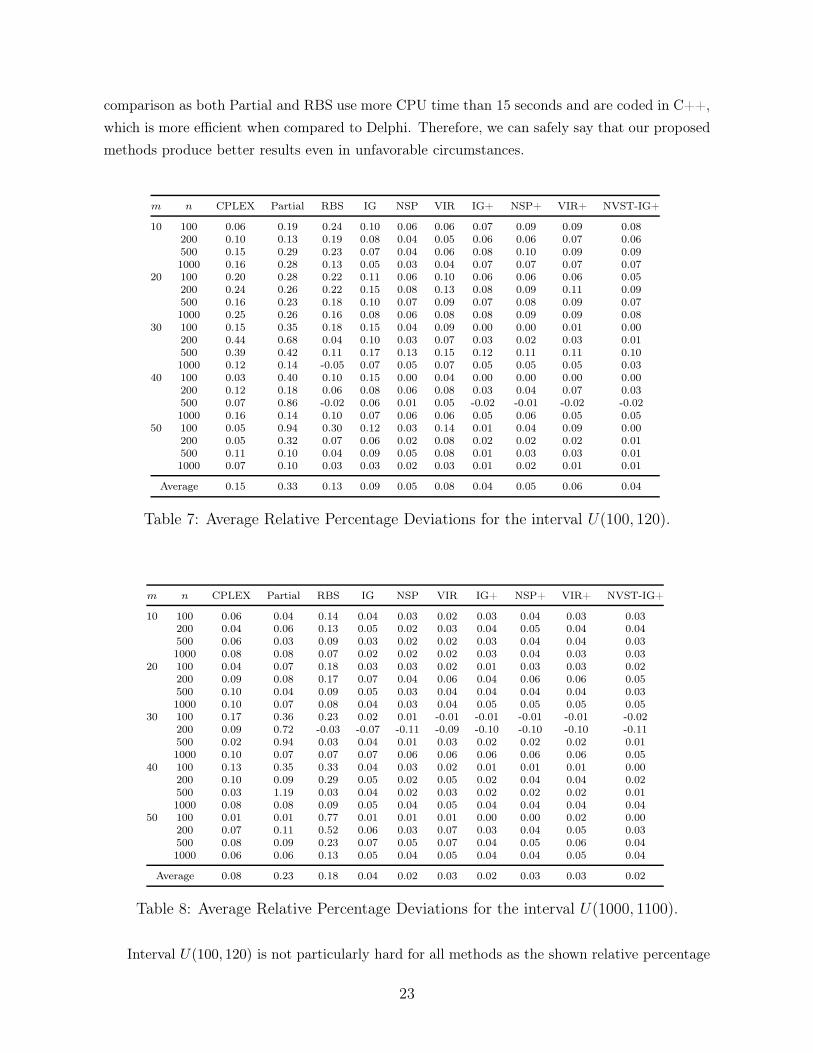
comparison as both Partial and RBS use more CPU time than 15 seconds and are coded in C++,

which is more efficient when compared to Delphi. Therefore, we can safely say that our proposed

methods produce better results even in unfavorable circumstances.

m n CPLEX Partial RBS IG NSP VIR IG+ NSP+ VIR+ NVST-IG+

10 100 0.06 0.19 0.24 0.10 0.06 0.06 0.07 0.09 0.09 0.08200 0.10 0.13 0.19 0.08 0.04 0.05 0.06 0.06 0.07 0.06500 0.15 0.29 0.23 0.07 0.04 0.06 0.08 0.10 0.09 0.091000 0.16 0.28 0.13 0.05 0.03 0.04 0.07 0.07 0.07 0.07

20 100 0.20 0.28 0.22 0.11 0.06 0.10 0.06 0.06 0.06 0.05200 0.24 0.26 0.22 0.15 0.08 0.13 0.08 0.09 0.11 0.09500 0.16 0.23 0.18 0.10 0.07 0.09 0.07 0.08 0.09 0.071000 0.25 0.26 0.16 0.08 0.06 0.08 0.08 0.09 0.09 0.08

30 100 0.15 0.35 0.18 0.15 0.04 0.09 0.00 0.00 0.01 0.00200 0.44 0.68 0.04 0.10 0.03 0.07 0.03 0.02 0.03 0.01500 0.39 0.42 0.11 0.17 0.13 0.15 0.12 0.11 0.11 0.101000 0.12 0.14 -0.05 0.07 0.05 0.07 0.05 0.05 0.05 0.03

40 100 0.03 0.40 0.10 0.15 0.00 0.04 0.00 0.00 0.00 0.00200 0.12 0.18 0.06 0.08 0.06 0.08 0.03 0.04 0.07 0.03500 0.07 0.86 -0.02 0.06 0.01 0.05 -0.02 -0.01 -0.02 -0.021000 0.16 0.14 0.10 0.07 0.06 0.06 0.05 0.06 0.05 0.05

50 100 0.05 0.94 0.30 0.12 0.03 0.14 0.01 0.04 0.09 0.00200 0.05 0.32 0.07 0.06 0.02 0.08 0.02 0.02 0.02 0.01500 0.11 0.10 0.04 0.09 0.05 0.08 0.01 0.03 0.03 0.011000 0.07 0.10 0.03 0.03 0.02 0.03 0.01 0.02 0.01 0.01

Average 0.15 0.33 0.13 0.09 0.05 0.08 0.04 0.05 0.06 0.04

Table 7: Average Relative Percentage Deviations for the interval U(100, 120).

m n CPLEX Partial RBS IG NSP VIR IG+ NSP+ VIR+ NVST-IG+

10 100 0.06 0.04 0.14 0.04 0.03 0.02 0.03 0.04 0.03 0.03200 0.04 0.06 0.13 0.05 0.02 0.03 0.04 0.05 0.04 0.04500 0.06 0.03 0.09 0.03 0.02 0.02 0.03 0.04 0.04 0.031000 0.08 0.08 0.07 0.02 0.02 0.02 0.03 0.04 0.03 0.03

20 100 0.04 0.07 0.18 0.03 0.03 0.02 0.01 0.03 0.03 0.02200 0.09 0.08 0.17 0.07 0.04 0.06 0.04 0.06 0.06 0.05500 0.10 0.04 0.09 0.05 0.03 0.04 0.04 0.04 0.04 0.031000 0.10 0.07 0.08 0.04 0.03 0.04 0.05 0.05 0.05 0.05

30 100 0.17 0.36 0.23 0.02 0.01 -0.01 -0.01 -0.01 -0.01 -0.02200 0.09 0.72 -0.03 -0.07 -0.11 -0.09 -0.10 -0.10 -0.10 -0.11500 0.02 0.94 0.03 0.04 0.01 0.03 0.02 0.02 0.02 0.011000 0.10 0.07 0.07 0.07 0.06 0.06 0.06 0.06 0.06 0.05

40 100 0.13 0.35 0.33 0.04 0.03 0.02 0.01 0.01 0.01 0.00200 0.10 0.09 0.29 0.05 0.02 0.05 0.02 0.04 0.04 0.02500 0.03 1.19 0.03 0.04 0.02 0.03 0.02 0.02 0.02 0.011000 0.08 0.08 0.09 0.05 0.04 0.05 0.04 0.04 0.04 0.04

50 100 0.01 0.01 0.77 0.01 0.01 0.01 0.00 0.00 0.02 0.00200 0.07 0.11 0.52 0.06 0.03 0.07 0.03 0.04 0.05 0.03500 0.08 0.09 0.23 0.07 0.05 0.07 0.04 0.05 0.06 0.041000 0.06 0.06 0.13 0.05 0.04 0.05 0.04 0.04 0.05 0.04

Average 0.08 0.23 0.18 0.04 0.02 0.03 0.02 0.03 0.03 0.02

Table 8: Average Relative Percentage Deviations for the interval U(1000, 1100).

Interval U(100, 120) is not particularly hard for all methods as the shown relative percentage

23

deviations are very close to zero. In this benchmark, CPLEX under two hours was capable of

solving a large number of instances and the observed gap in those that could not be solved was very

small. Still, once again, all our proposed methods are significantly better than the competition.

The best methods are IG+ and NVST-IG+ with average results of 0.04%. The best method from

the competition is RBS, with a 0.13%. In other words, our best proposed algorithms are at least

325% better than the competition. Lastly, for interval U(1000, 1100) we have a similar situation

where IG+ and NVST-IG+ are the best with 0.02% and the best competitor is CPLEX with

0.08%, i.e., 400% worse. We would like to point out that in these three new benchmarks, CPLEX

is significantly better than Partial and RBS is most cases.

In order to have a clear overall picture, Table 9 shows all seven tested benchmarks along with

all proposed methods, CPLEX, Partial and RBS. The table just gathers all previously presented

results.

Interval CPLEX Partial RBS IG NSP VIR IG+ NSP+ VIR+ NVST-IG+

U(1, 100) 1.88 2.88 2.03 2.46 2.82 2.3 1.68 2.10 1.95 1.34

U(10, 100) 1.64 1.31 1.87 1.7 1.56 1.45 0.94 1.19 1.11 0.75

U(100, 200) 0.76 1.05 0.81 0.52 0.36 0.45 0.35 0.38 0.42 0.32

U(100, 120) 0.15 0.33 0.13 0.09 0.05 0.08 0.04 0.05 0.06 0.04

U(1000, 1100) 0.08 0.23 0.18 0.04 0.02 0.03 0.02 0.03 0.03 0.02

jobcorre 2.20 2.43 0.35 1.08 0.54 0.71 0.59 0.40 0.63 0.48machcorre 1.13 0.94 2.36 0.66 0.59 0.58 0.60 0.56 0.56 0.55

Average 1.12 1.31 1.10 0.94 0.85 0.80 0.60 0.67 0.68 0.50

A. typical 1.71 1.89 1.65 1.48 1.38 1.26 0.95 1.07 1.06 0.78

A.typical= Average of more typical intervals: U(1, 100); U(10, 100); Jobs Correlated; Machines Correlated

Table 9: Summary results for all benchmarks and algorithms. Bold (italics) figures repre-sent best (worst) results, respectively.

We have calculated two global averages. The first one is the average results for each method

of all seven tested benchmarks, i.e., an average relative percentage deviation from the 2-hour

CPLEX reference solution for all 1,400 instances. The second global average contains the four

“typical” intervals, i.e.: U(1, 100), U(10, 100), Jobs Correlated, Machines Correlated. We show

the two averages in order to avoid a bias in the final results possibly due to our three new proposed

benchmarks. Looking at these averages we can see how all our seven proposed algorithms yield

better results than the competition in our computational settings. At this point, we have to re-

mark that our proposed methods are remarkably simple and make no use of commercial solvers.

Among all tested benchmarks, RBS manages to beat NVST-IG+ for job correlated instances.

However, RBS uses, on average, around 25 seconds of CPU time and NVST-IG+ has been run

for just 15 seconds. We will later show some additional results for longer CPU times.

So far we have just shown average results. We need to carry out some statistical testing in

order to guarantee that the observed differences in the average results are indeed statistically

24

significant. We carry out a Design of Experiments (DOE, Montgomery, 2009) where we study a

single factor, i.e., the type of algorithm at 10 levels and the average relative percentage deviation

is the response variable. We take all previous results where each instance is considered a treatment

and there are 1,400 results for CPLEX, Partial and RBS and 7,000 results (five replicates) for

each one of our seven proposed methods. Recall that in total there are 53,200 results. The results

of the DOE are analyzed by means of the single factor Analysis of Variance (ANOVA) technique.

We check the three main hypotheses of the parametric ANOVA: normality, homocedasticity and

independence of the residuals. With such a large set of results, the residuals from the ANOVA

easily satisfied all three hypotheses. Figure 7 shows the means plot with Tukey HSD intervals with

95% confidence level. Recall that overlapping intervals indicates that no statistically significant

difference exists among the overlapped means.

Relat

ive Pe

rcenta

ge D

eviat

ion (R

PD)

0. 46

0. 66

0. 86

1. 06

1. 26

1. 46

VIR+

NSP+IG

+

VIR

NSPIGRBS

Parti

al

CPLE

X

NVST

-IG+

Figure 7: Means plot and Tukey HSD intervals with 95% confidence level for all testedalgorithms and all instances.

As can be seen, Partial is indeed statistically worse than CPLEX. Of course, this applies to

the overall average. Notice that the Tukey intervals are fairly wide, which means that different

results could be observed by zooming in for each different benchmark. RBS and CPLEX are

statistically equivalent. All our seven proposed methods are statistically better than CPLEX,

Partial and RBS. However, NSP and VIR are equivalent. The same can be said about the im-

proved NSP+ and VIR+ versions. Finally, NVST-IG+ is statistically better than all other tested

methods.

25

All previous results have been carried out with all our seven proposed methods and CPLEX

stopping at 15 seconds CPU time. Recall that Partial is stopped after 15 CPU seconds have

elapsed in the second phase, and therefore the total time is larger. Recall also that the CPU time

of RBS is not controllable and therefore it has been run for an approximate overall average of

25 seconds. A final question remains. Are the good results of NVST-IG+ maintained with lower

or higher CPU time? We aim now at answering this question. We have carried out additional

experiments where the stopping CPU time has been set at 5, 25, 300, 600, 1,800, 3,600 and

7,200 seconds. Again, the exact times can only be controlled for CPLEX and our seven proposed

methods. These times are used for the second phase of Partial and only up to 300 seconds. RBS

has been tested at 25 seconds (more or less its natural stopping time, on average) and at 300

seconds after increasing the beam width. All these results are shown in Table 10.

Time Algorithms U(1, 100) U(10, 100) U(100, 200) U(100, 120) U(1000, 1100) Jobcorre Machcorre Average

5 Partial 3.93 2.25 1.22 0.36 0.27 2.89 1.49 1.77

CPLEX 3.45 2.53 0.98 0.20 0.09 3.92 2.70 1.98

NVST-IG+ 1.78 1.06 0.41 0.06 0.03 0.71 0.66 0.67

25 Partial 2.45 1.22 0.69 0.28 0.18 2.12 0.73 1.10

CPLEX 1.41 1.42 0.58 0.12 0.04 1.75 0.69 0.86

NVST-IG+ 1.20 0.61 0.27 0.04 0.02 0.38 0.51 0.43

RBS 2.03 1.87 0.81 0.13 0.18 0.35 2.36 1.10

300 Partial 1.59 0.33 0.20 0.21 0.09 1.23 0.10 0.54

CPLEX 0.35 0.29 0.24 0.04 0.02 0.45 0.12 0.22

NVST-IG+ 0.67 0.19 0.14 0.02 0.00 0.05 0.38 0.21

RBS 0.87 0.85 0.39 0.07 0.08 -0.20 1.17 0.46

600 CPLEX 0.24 0.20 0.17 0.03 0.01 0.27 0.07 0.14

NVST-IG+ 0.58 0.09 0.10 0.01 0.00 -0.02 0.35 0.16

1,800 CPLEX 0.12 0.11 0.08 0.02 0.01 0.12 0.03 0.07

NVST-IG+ 0.53 0.02 0.07 0.01 -0.01 -0.11 0.32 0.12

3,600 CPLEX 0.05 0.06 0.02 0.01 0.00 0.07 0.01 0.03

NVST-IG+ 0.49 -0.03 0.05 0.00 -0.01 -0.2 0.29 0.09

7,200 CPLEX 0.00 0.00 0.00 0.00 0.00 0.00 0.00 0.00

NVST-IG+ 0.38 -0.07 0.03 0.00 -0.01 -0.26 0.27 0.05

Table 10: Average results for the best methods and different CPU stopping criteria. Bold(italics) figures represent best (worst) results, respectively.

One striking result is that NVST-IG+ is the best method when run for an extremely short

amount of time (5 seconds) and the total average relative percentage deviation from the 2-hour

CPLEX solution is 0.67%. This is a 296% better than CPLEX and 264% better than Partial.

We think that these results are noteworthy since in just a mere 5 seconds, very good average

results can be obtained without using a solver. For 25 and 300 seconds, NVST-IG+ is still the

best method, on average. RBS improves significantly when compared to the 25 seconds stopping

26

time but does not manage to beat CPLEX or NVST-IG+. Partial is the worst method in all

tested cases (CPU time ≤ 300). As we can see, although all previous computational evaluations

were carried out with a 15 seconds CPU time limit, similar conclusions can be drawn with less

and more CPU time.

For longer processing times of 10, 30, 60 and 120 minutes, we have just compared the two

best methods, i.e., CPLEX and NVST-IG+. Overall, with more time, CPLEX gets obviously

better. After all, IBM-ILOG CPLEX 11.0. applies state-of-the-art Branch and Cut exact algo-

rithms and it is expected to beat any other method under extended CPU time. However, it is

quite remarkable how NVST-IG+ does not stall and steadily improves results across all instances.

Actually, for the interval U(1000, 1100) and where processing times are job correlated, NVST-

IG+ improves the results of the 2-hour CPLEX already for 10 minutes, which is quite remarkable.

As a matter of fact, we evaluate CPLEX vs. NVST-IG+ for even more different stopping

points. We carry out a two-factor ANOVA whose means interaction plot is shown in Figure 8.

Again, it must be noted that the means plot shows overall averages. We can observe that for

up to 60 seconds, it is, on average, better to use NVST-IG+ instead of CPLEX. From that

point and all the way up to two hours, it is statistically equivalent to employ CPLEX or NVST-

IG+. However, we can see how the curve of CPLEX falls below that of NVST-IG+ around 600

seconds. Therefore, for some specific benchmarks and instances, CPLEX is expected to provide

better results.

algorithmCPLEX

- 0 .1

0 .2

0 .5

0 .8

1 .1

1 .4

1 .7

5 15 30 60 120 240 300 600 1800 3600 7200

Relat

ive Pe

rcenta

ge D

eviat

ion (R

PD)

NVST-IG+

Figure 8: Means interaction plot and Tukey HSD intervals with 95% confidence level forCPLEX and NVST-IG+ and all instances.

27

5 Conclusions and future research

In this paper we have proposed seven new algorithms for the unrelated parallel machine scheduling

problem under makespan criterion or R//Cmax. The methods presented are remarkable simple

and are mainly composed of a very simple solution initialization, a Variable Neighborhood De-

scent loop (VND, Mladenovic and Hansen, 1997; Hansen and Mladenovic, 2001), and a solution

modification procedure. Three basic algorithms: IG, NSP and VIR have been initially presented.

Then we have improved these methods by selecting jobs and machines in a more smart way,

creating the improved IG+, NSP+ and VIR+ methods. Later, all the ideas have been joined in

a still remarkable simple NVST-IG+ method.

A comprehensive benchmark test of 1,400 instances has been employed in order to compare

all presented algorithms against state-of-the-art methods, identified as IBM-ILOG CPLEX 11.0.,

Partial of Mokotoff and Jimeno (2002) and RBS of Ghirardi and Potts (2005). An exhaustive

computational campaign has been carried out which has needed almost 4 years of CPU time. All

results have been statistically tested. In most situations, our presented algorithms have yielded

results that are statistically better, and by a significant margin, that the aforementioned state-

of-the-art procedures. We think that these results are remarkable specially if we consider the

inherent simplicity of the local search-based proposed methods. Other interesting results is that

recent versions of CPLEX are actually competitive, improving the results of Partial and RBS in

most situations.

Future research stems from the consideration of more elaborated neighborhood definitions

inside the VND loop, together with a further improvement in the selection of jobs and machines

which could further bolster results. We are also interested in applying the proposed techniques

to other more sophisticated parallel machines problems, like those resulting from the addition of

sequence dependent setup times and/or to other objectives, like those based on job’s due dates.

Acknowledgments

The authors are partly funded by the Spanish Department of Science and Innovation (research

projects ref. DPI2008-03511/DPI and IAP-020100-2008-11).

The authors would like to sincerely thank A. Woclaw and M. Ghirardi for their help and for

providing the valuable codes that have been employed in the computational evaluation of the

Partial and RBS methods.

28

References

Cheng, T. C. E. and Sin, C. C. S. (1990). A state-of-the-art review of parallel-machine schedulingresearch. European Journal of Operational Research, 47(3):271–292.

Davis, E. and Jaffe, J. M. (1981). Algorithms for scheduling tasks on unrelated processors.Journal of the ACM, 28(4):721–736.

De, P. and Morton, T. E. (1980). Scheduling to minimise makespan on unequal parallel processors.Management Science, 11(4):586–602.

de la Croce, F., Ghirardi, M., and Tadei, R. (2004). Recovering beam search: Enhancing the beamsearch approach for combinatorial optimization problems. Journal of Heuristics, 10(1):89–104.

Dillenberger, C., Escudero, L. F., Wollensak, A., and Wu, Z. (1994). On practical resource-allocation for production planning and scheduling with period overlapping setups. European

Journal of Operational Research, 75(2):275–286.

Gairing, M., Monien, B., and Woclaw, A. (2007). A faster combinatorial approximation algorithmfor scheduling unrelated parallel machines. Theoretical Computer Science, 380(1-2):87–99.

Garey, M. R. and Johnson, D. S. (1979). Computers and intractability: A guide to the theory ofNP-completeness. Freeman. San Francisco.

Ghirardi, M. and Potts, C. N. (2005). Makespan minimization for scheduling unrelated parallelmachines: A recovering beam search approach. European Journal of Operational Research,165(2):457–467.

Glass, C. A., Potts, C. N., and Shade, P. (1994). Unrelated parallel machine scheduling usinglocal search. Mathematical and Computer Modelling, 20(2):41–52.

Graham, R. L. (1969). Bounds on multiprocessing timing anomalies. SIAM Journal on Applied

Mathematics, 17(2):416–429.

Graham, R. L., Lawler, E. L., Lenstra, J. K., and Rinnooy Kan, A. H. G. (1979). Optimizationand approximation in deterministic sequencing and scheduling: A survey. Annals of Discrete

Mathematics, 5:287–326.

Hansen, P. and Mladenovic, N. (2001). Variable neighborhood search: Principles and applications.European Journal of Operational Research, 130(3):449–467.

Hariri, A. M. A. and Potts, C. N. (1991). Heuristics for scheduling unrelated parallel machines.Computers & Operations Research, 18(3):323–331.

Horowitz, E. and Sahni, S. (1976). Exact and approximate algorithms for scheduling nonidenticalprocessors. Journal of the ACM, 23(2):317–327.

Ibarra, O. H. and Kim, C. E. (1977). Heuristic algorithms for scheduling independent tasks onnonidentical processors. Journal of the ACM, 24(2):280–289.

Lenstra, J. K., Rinnooy Kan, A. H. G., and Brucker, P. (1977). Complexity of machine schedulingproblems. Annals of Discrete Mathematics, 1.

Lenstra, J. K., Shmoys, D. B., and Tardos, E. (1990). Approximation algorithms for schedulingunrelated parallel machines. Mathematical Programming, 46(3):259–271.

Mansini, R. and Speranza, M. G. (1999). Heuristic algorithms for the portfolio selection problemwith minimum transaction lots. European Journal of Operational Research, 114(2):219–233.

Martello, S., Soumis, F., and Toth, P. (1997). Exact and approximation algorithms for makespanminimization on unrelated parallel machines. Discrete Applied Mathematics, 75(2):169–188.

McNaughton, R. (1959). Scheduling with deadlines and loss functions. Management Science,6(1):1–12.

Mladenovic, N. and Hansen, P. (1997). Variable neighborhood search. Computers & Operations

Research, 24(11):1097–1100.

29

Mokotoff, E. (2001). Parallel machine scheduling problems: A survey. Asia-Pacific Journal of

Operational Research, 18(2):193–242.

Mokotoff, E. and Chretienne, P. (2002). A cutting plane algorithm for the unrelated parallelmachine scheduling problem. European Journal of Operational Research, 141(3):515–525.

Mokotoff, E. and Jimeno, J. L. (2002). Heuristics based on partial enumeration for the unrelatedparallel processor scheduling problem. Annals of Operations Research, 117(1-4):133–150.

Montgomery, D. C. (2009). Design and Analysis of Experiments. Wiley, New York, seventhedition.

Ow, P. S. and Morton, T. E. (1988). Filtered beam search in scheduling. International Journal

of Production Research, 26(1):35–62.

Piersma, N. and van Dijk, W. (1996). A local search heuristic for unrelated parallel ma-chine scheduling with efficient neighborhood search. Mathematical and Computer Modelling,24(9):11–19.

Pinedo, M. L. (2005). Planning and Scheduling in Manufacturing and Services. Springer Seriesin Operations Research. Springer, New York, USA.

Pinedo, M. L. (2008). Scheduling: Theory, Algorithms, and Systems. Springer, New York, USA,third edition.

Potts, C. N. (1985). Analysis of a linear-programming heuristic for scheduling unrelated parallelmachines. Discrete Applied Mathematics, 10(2):155–164.

Ruiz, R. and Stützle, T. (2007). A simple and effective iterated greedy algorithm for the permu-tation flowshop scheduling problem. European Journal of Operational Research, 177(3):2033–2049.

Ruiz, R. and Stützle, T. (2008). An iterated greedy heuristic for the sequence dependent setuptimes flowshop problem with makespan and weighted tardiness objectives. European Journal

of Operational Research, 187(3):1143–1159.

Shchepin, E. V. and Vakhania, N. (2005). An optimal rounding gives a better approximation forscheduling unrelated machines. Operations Research Letters, 33(2):127–133.

Shmoys, D. B. and Tardos, E. (1993). An approximation algorithm for the generalized assignmentproblem. Mathematical Programming, 62(3):461–474.

Sourd, F. (2001). Scheduling tasks on unrelated machines: Large neighborhood improvementprocedures. Journal of Heuristics, 7(6):519–531.

Srivastava, B. (1998). An effective heuristic for minimising makespan on unrelated parallel ma-chines. Journal of the Operational Research Society, 49(8):886–894.

Sule, D. R. (2008). Production Planning and Industrial Scheduling: Examples, Case Studies and

Applications. CRC Press, Boca Raton, USA, second edition.

van de Velde, S. L. (1993). Duality based algorithms for scheduling unrelated parallel machines.ORSA Journal on Computing, 5(5):192–205.

Woclaw, A. (2006). Scheduling Unrelated Parallel Machines. Algorithms, Complexity, and Perfor-

mance. PhD thesis, Fakultat fur Elektrotechnik, Informatik und Mathematik der UniversitatPaderborn, Deutschland.

30