ISTITUTO DI STUDI E ANALISI ECONOMICA

Pricing to market when quality matters

by

Roberto Basile Institute for Studies and Economic Analyses (ISAE)

Piazza dell’Indipendenza, 4, 00185 Roma, Italia e-mail: r.basile@isae.it

Sergio de Nardis Institute for Studies and Economic Analyses (ISAE)

Piazza dell’Indipendenza, 4, 00185 Roma, Italia e-mail: s.denardis@isae.it

Alessandro Girardi Institute for Studies and Economic Analyses (ISAE)

Piazza dell’Indipendenza, 4, 00185 Roma, Italia e-mail: a.girardi@isae.it

Working paper n. 123 December 2009

The Series “Documenti di Lavoro” of the Istituto di Studi e Analisi Economica – Institute for Studies and Economic Analyses (ISAE) hosts the preliminary results of the research projects carried out within ISAE. The diffusion of the papers is subject to the favourable opinion of an anonymous referee, whom we would like to thank. The opinions expressed are merely the Authors’ own and in no way involve the ISAE responsability.

The series is meant for experts and policy-makers with the aim of submitting proposals and raising suggestions and criticism.

La serie “Documenti di Lavoro” dell’Istituto di Studi e Analisi Economica

ospita i risultati preliminari di ricerche predisposte all’interno dell’ISAE: La diffusione delle ricerche è autorizzata previo il parere favorevole di un anonimo esperto della materia che qui si ringrazia. Le opinioni espresse nei “Documenti di Lavoro” riflettono esclusivamente il pensiero degli autori e non impegnano la responsabilità dell’Ente.

La serie è destinata agli esperti e agli operatori di politica economica, al fine di formulare proposte e suscitare suggerimenti o critiche.

Stampato presso la sede dell’Istituto

ISAE - Piazza dell’Indipendenza, 4 – 00185 Roma. Tel. +39-06444821; www.isae.it

ABSTRACT We build a model of price differentiation with firm heterogeneity, which

allows for imperfect competition and market segmentation in the presence of flexible exchange rates as well as horizontal and vertical differentiation and different tastes of consumers in destination markets. We empirically assess the main predictions of our theoretical framework by using firm-level data surveyed by ISAE. We document that export-domestic price margins are significantly affected by price and quality competitiveness even controlling for foreign demand conditions, size, export intensity, destination markets and unobservables. Finally, we provide evidence of a strong heterogeneity across firms in their reaction to price and quality competitiveness.

Keywords: Pricing to market, qualitative choice models, firm heterogeneity.

JEL codes: D21, F10, C23, C25.

NON TECHNICAL SUMMARY An abundant bulk of empirical evidence shows that exporting firms move

price of their goods differently according to destination markets. In search for causes leading to price diversification, analysts have long focused on exchange rate swings: firms modify their markup and price of a given good according to the destination markets where it is sold, as an optimal response to some fundamental change in market-specific competitive pressures (pricing-to-market, PTM).

Since price differentiation according to markets is by now common wisdom for international economists, an interesting question is how this consolidated proposition relates with the literature on firm heterogeneity and international trade: is PTM behaviour obtainable from models of firm heterogeneity? Does the fact that firms are heterogeneous in productivity exert any influence in differentiating their capacity to modify prices according to markets?

In this paper we investigate these issues by developing a a model of PTM where firms move the margin between export and domestic prices of the same good in response to country-specific shocks to price and quality competition factors, with the latter identified by market-specific shifts in consumers’ tastes for quality. Besides predicting classic PTM results (e.g., reduction of the price made in a particular market as price competition in that market gets tougher), the model allows to cast some light on the consequences for pricing practices when quality matters. Provided a firm sells a variety of a good whose quality is better than the average of competitors faced in a given country, it rises its price whenever consumers’ preferences for quality intensify in that market. Moreover we have shown that, if quality has a role, the response to given destination-specific shocks to price and quality competition is affected by firm heterogeneity: higher-quality firms react more strongly to shifts in price competition than lower quality producers. Also the response to changes in tastes for quality may be stronger for higher-quality firms; actually this is always the case when such firms rank higher than the average quality of competitors.

We have tested the model against a dataset on a sample of Italian firms finding confirmation of the basic predictions of the model: Italian exporters do practice PTM strategies in response to shifts in price competition in foreign markets; they set higher export prices as competition on quality intensifies in foreign outlets, denoting a better quality level than competitors; those producers characterised by higher quality are capable to practice stronger PTM, reacting to shocks to both price and quality competition, than the lower-quality ones.

PRICING TO MARKET E IL RUOLO DELLA QUALITÀ

SINTESI In questo lavoro si presenta un modello teorico per lo studio

dell’eterogeneità nelle politiche di prezzo delle imprese esportatrici in presenza competizione imperfetta, segmentazione dei mercati, tassi di cambio flessibili, differenziazione orizzontale e verticale ed eterogeneità nei gusti dei consumatori nei mercati di destinazione. Le principali implicazioni dello schema teorico sono valutate empiricamente utilizzando dati trimestrali a livello di impresa raccolti dall’ISAE. I risultati suggeriscono che il margine tra prezzo praticato all’estero e quello praticato sul mercato interno (per lo stesso bene) è fortemente influenzato da fattori di costo e di qualità, anche tenendo conto dell’effetto delle condizioni cicliche dell’economia, della dimensione di impresa, dell’orientamento all’export, dei mercati di destinazione e di altri fattori di eterogeneità non osservabile. Infine, si mostra l’esistenza di una forte eterogeneità tra le imprese del campione in riferimento alla loro reazione ai fattori di competitività di prezzo e di qualità

Parole chiave: Pricing to market, modelli per dati qualitativi, eterogeneità di impresa.

Classificazione JEL: D21, F10, C23, C25.

CONTENTS

1 INTRODUCTION ................................................................................ 7

2 THEORETICAL FRAMEWORK ................................................... 12

2.1 Demand ....................................................................................... 12

2.2 Supply .......................................................................................... 14

2.3 Pricing policies ........................................................................... 18

3 FROM THEORY TO EMPIRICS .................................................. 21

3.1 Hypotheses to test .................................................................... 21

3.2 Data .............................................................................................. 23

3.3 Econometric framework ............................................................ 26

4 RESULTS .......................................................................................... 29

4.1 Pooled ORMs estimation results ........................................... 30

4.2 Random parameters ORMs estimation results .................. 32

5 CONCLUSIONS ............................................................................... 37

APPENDIX ........................................................................................ 38

References ............................................................................................... 41

7

1 INTRODUCTION1

An abundant bulk of empirical evidence shows that exporting firms move price of their goods differently according to destination markets. In search for causes leading to price diversification, analysts have long focused on exchange rate swings. In their pioneering works, Dornbusch (1987) investigates pricing strategies drawing on models of industrial organization, while Krugman (1987) formalizes them with the concept of pricing-to-market (PTM)2. Irrespective of whether a partial equilibrium framework (besides the cited works, Baldwin, 1988; Marston 1990) or a general equilibrium approach (Betts and Devereux, 1996; Corsetti et al., 2005) is adopted, what is presumed in these models is that a firm modifies markup and price of a given good according to the destination markets where it is sold, as an optimal response to some fundamental change in market-specific competitive pressures (epitomized by exchange-rate movements)3.

Since price differentiation according to markets is by now common wisdom for international economists, an interesting question is how this consolidated proposition relates with the literature on firm heterogeneity and international trade: is PTM behaviour obtainable from models of firm heterogeneity? Does the fact that firms are heterogeneous in productivity exert any influence in differentiating their capacity to modify prices according to markets? In this paper we investigate these issues. Main contribution is threefold. First, we uncover the PTM behaviour of exporters that is implicit in one of the basic models of firm heterogeneity and international trade. Second, we show that PTM policies pursued by firms take place not only in reaction to shifts in price competition, but also in response to movements in non-price competitiveness factors, such as taste for quality of consumers in destination markets. Finally, we point out that, provided that quality has a role, there is heterogeneity in firms’ capability to move prices in response to market-specific shocks to competition: higher-quality

1 We would like to thank Giuseppe De Arcangelis, Antonella Nocco and participants at the Conference

“Italy’s External Competitiveness” (Ministry of the Economy and Finance, Rome, 24-25 Novemder 2009) for their helpful comments.

2 If the domestic currency appreciates, a firm reacts by reducing the domestic currency price of the good sold abroad to restrain the rise of the corresponding foreign price and the consequent fall of the (volume) market share. Acording to these approaches, incentives at limiting the market share loss relate to the long-run investment made to establish in the market and the adjustment costs the firm has to incur when reducing volume of sales (Froot and Klemperer, 1989; Kasa, 1992).

3 For comprehensive surveys on PTM and the related phenomenon of incomplete exchange-rate pass-through, see Goldberg and Knetter (1997) and Campa and Goldberg (2005).

8

producers are able to practice PTM more than lower-quality firms, thanks to greater market power. The two latter results are quite novel in the literature dealing with, respectively, PTM and firm-heterogeneity. We use an original dataset providing information on firm-level pricing behaviour and apply an appropriate econometric framework when putting the model into empirical test.

Studying firm-level price differentiation policies requires a theoretical setting characterized by: 1) imperfect competition, 2) market segmentation and 3) variable price elasticity of demand in destination markets. While the first two conditions are necessary to enable different price levels in different markets, only the third one leads to what is commonly defined a PTM policy. Among the models of international trade and firm heterogeneity, the one by Melitz and Ottaviano (2008) (MO, from now on) presents all the required features: firms operate under monopolistic competition, markets are not fully integrated because of the existence of trade costs and, crucially, markups are not constant, but depend on the specific characteristics (toughness of competition) of each destination market. Although this model does not tackle the issue of pricing policies according to markets, except for the prediction of price-level discrimination in reciprocal dumping, it lends itself quite naturally to study PTM and, with some extensions, it allows to cast light on the consequences on firms’ behaviour when product quality affects pricing decisions.

Other recent open-economy models consider variable markups and firm heterogeneity. Bernard et. al. (2003) build up a Ricardian framework with endogenous markups; yet invariance of markup distribution across destination markets makes this model unfit for analyzing PTM policies. Atkeson and Burstein (2008) use a nested CES demand system to study movements in international relative prices stemming from PTM of firms facing aggregate shocks: markup is variable, in this case, if goods within the same sector are more substitutable than goods between different sectors. This is a proper PTM model giving rise to heterogeneity of firms’ pricing behaviour in destination markets as markups respond to changes of firms’ market shares that differ at home and abroad. The use of a variant of the standard CES-preference structure imposes, however, conditions on the model, limiting generality of PTM results. Also Berman et al. (2009) start from a standard constant-elasticity Dixit-Stiglitz framework. In this model, variability of markup in destination markets is ensured by the introduction of country-specific distribution costs (on top of fixed and trade costs). The latter make the perceived demand elasticity to producer’s price variable according to markets and dependent on firm heterogeneity: high performance firms perceive lower demand elasticity and are hence able to practice PTM more than the low performance ones. A different theoretical perspective is adopted by Auer and Chaney (2008) who study firm-level pricing

9

policies under perfect competition and flexible prices. Producers sell goods of different quality content to consumers having heterogeneous preferences for quality; exchange rate shocks affect both the intensive and extensive margins of exporters in the relevant market leading to incomplete exchange-rate pass-through and heterogeneous price responses of producers to currency shocks: high-quality firms are capable to limit the pass-through of exchange rate on final consumers more than the low-quality ones.

In our work we follow a different route from these papers by considering the more general framework of endogenous distribution of market-specific markups delivered by the MO model, where price differentiation and PTM behaviour stem out as natural outcomes of the basic setting. Besides making explicit the influence of exchange rates in diversifying price-setting conditions in domestic and foreign markets, we modify the framework proposed by MO along two directions: i) consumers are characterized not only by preference for variety, but also by love for quality, so that their utility rises with quality-augmented quantities of differentiated varieties; ii) such preferences are not uniform across markets, but vary from one country to another. The way we treat country-specific quality taste is similar to the one proposed by Hallak (2006), although we incorporate it within a different preference structure.

Introduction of quality evaluation on the demand side implies the existence of a mechanism of quality generation of goods on the supply side. We adopt the simple rule proposed by Baldwin and Harrigan (2007), featuring a direct link between marginal cost and quality content of varieties. Other recent studies based on the MO framework, such as that by Antoniades (2008), develop models of endogenous choice of the quality content of goods to investigate why some firms embark in quality upgrading and some others stay in the low segment; also Borin (2008) offers a framework of endogenous quality determination. For the purpose of our study, aiming at explaining pricing policies of firms across markets, we rely on the simpler quality generation mechanism suggested by Baldwin-Harrigan as it works just as a (necessary) support to have price differentiation: a single variety has the same quality content wherever it is sold; what matters is the possibility that consumers in different countries have different valuations of its quality attribute. The approach we adopt shares with the endogenous-quality models the basic prediction that, in presence of quality improvement, prices increase with productivity. This prediction emerges, through quite different channels, also from other studies introducing quality production and consumption into heterogeneous-firm models, such as those of Verhoogen (2008) analysing export-induced quality upgrading and of Kugler and Verhoogen (2008) testing complementarity between input quality, plant productivity and output quality.

10

The theoretical framework we propose allows to derive a whole range of responses to market-specific changes in price and non-price (quality) competitiveness factors. As price competition becomes tougher in a destination market, due to exchange rate appreciation and/or to lower price of competitors, firms reduce their markup and fob price in that market: this is the classic PTM (and incomplete exchange-rate pass-through) case dealt with by international macro-models; it derives from the increase of demand elasticity to fob price caused by fiercer price competition. As for market-specific quality factors, we show that when consumers’ tastes for quality rise, firms may either increase or reduce fob prices in the relevant destination market: it depends on the relative quality of their products with respect to the average of competitors. If it is higher than the average, then the rise of consumers’ quality preference causes a reduction of demand elasticity to fob price and induces an increase of price in the relevant market. If it is lower, there is an increase of demand elasticity and firm responds by reducing the price practiced in that country: a rise in quality taste in a destination market has an effect comparable to tougher competition for a firm producing a variety characterised by a lower-than-average quality content.

Firm heterogeneity influences the variation of fob-price in reaction to changes of price and quality competitiveness factors in a way dependent on the value of the quality variables. When quality has no role, we are in the basic MO case: the response to changes in price competition is independent of producer heterogeneity. Firm heterogeneity becomes relevant for price setting when quality matters. In this case, the reduction of fob prices in response to more intense price competition is stronger for firms producing higher quality goods. Relevant corollary is that high-quality products are characterized by lower exchange rate pass-through than low-quality products: this is consistent with the prediction made, in a different theoretical context, by Auer and Chaney (2008) and by Berman et al. (2009).

As for reaction to changes in quality tastes, the positive response of fob price practiced by firms producing goods whose quality is above the average of competitors gets even more positive for producers selling higher quality goods. Instead the negative response of fob prices adopted by firms producing below-the-average goods may become less or more negative, as quality content rises across firms, depending on the distance of the firm from the average quality of competitors and the intensity of preference for quality of consumers in destination market.

We test the model against data on Italian firms, making use of a longitudinal survey-dataset which gives consistent information on the pricing policy pursued by the firm (the margin between the price charged in foreign

11

markets and the price practiced domestically), the price and quality competitiveness factors faced by the firm in international markets, plus several firm-level control factors. The estimation results document that export-domestic price margins are indeed significantly affected by both price and quality competitive factors even controlling for foreign and domestic demand conditions, export intensity, destination markets and unobservables. Furthermore, a random parameter specification gives support to the hypothesis that, when quality matters, there is a strong heterogeneity in the pricing behaviour of firms, with the higher-quality ones being endowed with more market power and able to react in their price setting more strongly to modification in price and quality competition in destination markets.

Our paper is related to the literature analysing the differentiation of fob prices across destination markets, as in Hummels and Skiba (2004) and Johnson (2007), although the focus of our interest is rather different: while these works deal mainly with the question of why the “good apples are shipped out” (or, in different terms, why firms selling in faraway markets charge higher prices than those selling in nearby destinations), we consider the issue of why a firm can price the same apple differently across destination countries. Under this perspective our paper is more closely related to recent works studying the role of quality in firm-level price discrimination according to markets. Kneller and Yu (2008) analyse Chinese exporters’ behaviour and propose a model of heterogeneous firms with quality differentiation similar to ours: quality is added in the MO preference structure and is generated on the production side by the Baldwin-Harrigan rule. However, they do not consider the possibility of different quality preferences in destination countries and leave unspecified the parameterization of cost distribution. Both features are instead relevant in our model, where market-specific tastes for quality are the key element for quality to have a role in affecting price discrimination and in making it dependent on firm heterogeneity, and where explicit parameterization of cost distribution allows to get a precise characterization of price and quality components included in the competition variable (that is, quality-adjusted average price of competitors). Also Manova and Zhang (2009) study price discrimination practices of Chinese exporters. They suggest that the evidence, at odds with extant theories, that Chinese firms set higher prices in larger and more distant markets could be related to destination-specific quality-upgrading of goods taking place within the firm as a consequence of competition (which is tougher in larger and more distant markets). Although we do not tackle these issues, in our model increasing distance (e.g. higher bilateral transport cost an exporter incurs to deliver a good in a destination market) has the univocal effect of reducing fob export price, since it makes price competition tougher for exporters in the

12

destination country; when quality has a role, it is to enlarge the fob-price negative response to increasing distance. Apart from price-competition influences, in our model the possibility for a firm to charge higher prices in a destination market relative to other outlets (including the domestic one) resides not on how faraway is that market, but on how intense is the quality taste of consumers of that market relative to the quality preferences of consumers located in the other destinations.

The paper is structured as follows. In section 2 we introduce the theoretical framework used to model pricing behaviour of exporting firms. Dataset characteristics are illustrated in Section 3. Section 4 reports the empirical specification and estimation results. Section 5 concludes.

2 THEORETICAL FRAMEWORK

2.1 Demand

As in MO, consumers’ preferences are defined over a continuum of differentiated varieties and a homogenous product acting as numeraire. We modify this basic structure by assuming that, besides preference for variety, consumers have love for quality too: their utility rises with quality-augmented quantities of differentiated goods. Moreover we suppose, as in Hallak (2006), that consumers’ tastes differ from one country to another. Geographical differences in tastes may arise for a number of reasons. The most obvious one is that preferences are affected by per capita income levels which are different across countries4. This involves the possibility of variations of tastes both in space and time: consumers of richer economies are characterised by more intense love for quality and variety than consumers of poorer countries; consumers of catching up economies may increase over time their love for quality and horizontal differentiation filling the gap with the preference structure of advanced economies.

Preferences of the representative consumer in a generic country l are expressed as: 4 Empirical literature provides supporting evidence for the hypothesis that preferences for quality vary

across countries, see e.g. Hummels and Klenow (2005) and Choi et al. (2009). Crinò and Epifani (2008) explicitely link preference for quality to per-capita income to study the relationship between productivity, quality and export intensity to countries at different development levels.

13

( ) ( )22

, , , ,2 2l l ll

l l n j j l j j j l j j j l jU q z q dj z q dj z q djδ δ δ∈Ω ∈Ω ∈Ω

γ η= + α − −∫ ∫ ∫

where ,l nq and ,l jq are the quantities consumed of the homogeneous good,

indexed by n , and of the differentiated goods, indexed by j ∈ Ω ; jz is the

quality level of the differentiated goods; parameter 0 1l≤ δ ≤ is the intensity of

preference for quality of consumers in country l ; lγ measures love for (quality-

adjusted) variety in country l ; α and η measure the degree of substitution between differentiated varieties and the homogenous good. Parameters , , lα η γ

are assumed strictly positive. While α and η are equal across markets, lγ

and lδ are country-specific: the higher they are, the more intense are

preferences of country- l consumers respectively for variety and quality. Notice that having 0l >δ is not sufficient for quality to affect the utility level; it is also

necessary that the relevant variety has indeed a qualitative attribute, that is 1jz > 5. Quality content of goods is determined on the supply side.

Total expenditure of the representative consumer of country l is given by

, , ,l l n l j l jjS q p q dj

∈Ω= + ∫ , where ,l jp is the cif price that consumer of country l

pays for a specific variety j . Indexing by o the country where the firm

producing the j -th variety is located, , , , ,, o l j o l o ll jp p E= τ where , ,o l jp is the fob

price of variety j expressed in the currency of country o and sold in country l ,

,o lE is the exchange rate of the currency of country l for 1 unit of currency of

country o (and , ,1o l l oE E= ), ,o lτ is the transport cost (in iceberg-like form) a

firm incurs in transferring 1 unit of variety j from o to l ; these costs are assumed symmetric, so that , ,o l l oτ = τ . Moreover, when l o= ,

, , , , 1l l o o l l o oE E= = τ = τ = and , , ,l j o l jp p= .

Optimisation of preferences leads to the demand for quantity of variety j

in country l , which is linear for given quality level:

5 By the same token, having a qualitative attribute, 1jz > , is not sufficient for quality to affect utility; it is

necessary that consumers appreciate quality, 0lδ > , so that both terms co-determine consumers’

valuation of firm j’s product.

14

( ),

, , , ,l j l l l

o l j o l o ldem l l l l

l j l l l j j

p EL P Lqz N z zδ δ δ

τ′αγ + η= −

γ γ + η γ (1)

where lL is the number of consumers in country l ; lN is the number of

varieties consumed in country l coinciding with the number of competitors;

l

ll

PPz δ

′ = is the quality-adjusted average cif price across all varieties sold by

competitors in country l 6. The maximum quality-adjusted (cif) price in the l -country currency, at which demand for variety j zeroes, is:

, , , ,

max( )l

o l j o l o l l ll

j l l

p E P Mz Nδ

⎛ ⎞τ ′αγ + η= =⎜ ⎟⎜ ⎟ γ + η⎝ ⎠

(2)

2.2 Supply

Labour is the only input of production and firms draw quality-adjusted unit labour coefficients ja′ from a random distribution ( )G a′ having support on

[0, ]ma′ . Coefficients ja′ measure the amount of labour input, jL , necessary to

produce 1 unit of quality-adjusted output of variety j that is

j j j j j ja L q z a z′ = = . With unitary wage, ja′ coincides with quality-adjusted

marginal cost. Once unit labour coefficient is drawn, assessment of firm’s profitability in each market requires to weight the quality component of technology ( jz ) by the country-specific quality-taste parameter ( lδ ), that is

,l

l j j ja a zδ′ = . This is because different preferences for quality affect the cutoff

quality-adjusted marginal cost that firms face in each market, impacting their destination-specific profits. Particularly, a firm located in o and selling variety j

6 In (1) , , ' ''

ll c l j jj

P p z djδ

∈Ω′ ′= ∫ , where , , 'c l jp is the price of variety 'j j≠ made by competitors

in l . Note that in (1) the higher is quality, the higher is quantity demanded since

, , , , ,

2 2dem

l j o l j o l o ll lll l

l jj j

Lz

q p EM

z zδ δδ

γ

∂ τ= −

∂

⎛ ⎞⎜ ⎟⎝ ⎠

, where the term in parenthesis is positive since from (3)

, , , ,2 o l j o l o l j

l llj j

p E aM

z zδ δ

τ= + .

15

both in o and l faces a cutoff quality-adjusted marginal cost , o

oo o

o

aazδ

′ = in the

domestic market and a cutoff quality-adjusted marginal cost ,o la′ in the export

market; where ,,

, ,

l lo l

o l o l

aa

E′

′ =τ

and ,l la′ is the cutoff quality-adjusted marginal cost

(weighted by the quality taste of consumers and expressed in terms of currency

of country l ) faced by firms located and selling in l , that is , l

ll l

l

aazδ

′ = . The

cutoff cost ,o la′ coincides with the zero-demand (quality-adjusted and taste-

weighted) price threshold characterising market l , converted in currency of

country o and divided by transport costs: ,, ,

lo l

o l o l

MaE

′ =τ

. A firm will hence earn

positive profits (and will be selling) in markets o and l if , ,o j o oa a′ ′< and

, ,l j o la a′ ′< 7.

To determine jz , we assume, along with Baldwin and Harrigan (2007),

that the quality parameter is linked to marginal costs in a way such that, for any

variety j , j jz aθ= , where 0θ ≥ is an elasticity index: when 0θ = , quality is

inelastic to marginal costs and plays no role; when 0 1< θ < , quality rises with marginal costs, but less than proportionally; when 1θ ≥ an increase in marginal

costs induces no rise ( )1θ = or even a reduction ( )1θ > in quality-adjusted

marginal cost. Taking into account market-specific tastes yields 1,

ll j ja a −θδ′ = .

A profit maximising firm located in o and selling variety j in market l behaves as a monopolist which faces the residual demand function (1). Endowed with a randomly drawn technology, the firm takes the average

(quality-adjusted) price across varieties ( lP ′ ) and the number of competitors

( lN ) as given and adopts a pricing rule that sets the quality-unadjusted fob

7 Profits earned in markets o and l , in terms of currency of country o , are given respectively by

( )2

, , ,4o

o o o o o jo

L a aπγ

′ ′= − and ( )2

, , ,4l

o o o l l jl

L a aπγ

′ ′= − .

16

price, , ,o l jp , as a markup, , ,

, ,

, ,, ,

2l

o l jo l j

jo l j l

o l o l

pz

p ME

δμ =−

τ

, over the (quality-

unadjusted) marginal cost. The profit optimising fob price is hence the following:

, ,, , 2

lj

l jo l o l

o l j

aM a

Ep

θδ

+τ

= (3)

In free entry equilibrium, with expected profits driven to zero, adopting the assumption of a Pareto parameterization for technology distribution

( )k

m

aG aa

⎛ ⎞′′ = ⎜ ⎟′⎝ ⎠

, with 1k ≥ as shape parameter, and supposing that firms in

countries o and l share the same entry cost wherever they sell, (3) may be written as8.

1 12 2 21,

, ,

1 11

2

l

l

kk k k

lo l j jk

l mo l j

a aL a

p

θδθδ

γφ ττ

+ + +−

−

⎛ ⎞ ⎛ ⎞ ⎛ ⎞ +⎜ ⎟ ⎜ ⎟ ⎜ ⎟+⎝ ⎠⎝ ⎠ ⎝ ⎠= (4)

where , ,o l l oτ = τ = τ and 1

22( 1)( 2)( )k km entryk k a f +⎡ ⎤+ +⎣ ⎦φ = is a constant given

by the combination between Pareto distribution parameters and the fixed entry cost, entryf .

In (4), the fob price set in country l depends on firm-specific marginal

costs ( )ja and destination-specific variables, e.g. market dimension, l lLγ ,

and consumers’ preference for quality, lδ . Toughness of competition is affected by market dimension, which varies inversely with the degree of horizontal differentiation, lγ , and directly with the size of the country, lL : the larger is the dimension of destination markets, the more severe is competition, the lower is the average price practiced by competitors. Even trade barriers, represented by

8 Expression (4) comes from setting expected profits of producers located in the two countries and

selling in the two markets equal to the entry costs (which are the same for all producers in all markets); see Appendix.

17

the term ( )1

21 k k−− ++ τ , impact on the degree of competition inducing lower fob-

price as τ reduces. The assumed technology parameterization and the zero-profit condition

yield an explicit link between average quality-adjusted price (in currency of country o ) and market dimension (and trade barriers)9:

1 12 2 2

,

2 1 1 12( 1) 1l l

kk k k

l lk

o l l l m

P kE a k L a

+ + +

−

⎛ ⎞ ⎛ ⎞+ ⎛ ⎞= ⎜ ⎟ ⎜ ⎟ ⎜ ⎟+ +⎝ ⎠⎝ ⎠ ⎝ ⎠θδ θδ

γ φτ

(5)

We can use (5) to disentangle the influence of price competition from that of quality competition expressing (4) as:

,

, , 2

lVl j

jl

o l j

aK a

Cp+

=

%

(6)

where( )2 12 1

kK

k+

=+

; ,,

o ll o l

l

EC

Pτ= ; l lV = δ θ ; ,

jl j

l

aa

a⎛ ⎞

= ⎜ ⎟⎝ ⎠

% , where la is the

average marginal cost across competitors in market l . Underlying the price setting (6) there is an elasticity of demand to quality-

unadjusted fob price faced by a producer selling variety j in destination l given, in absolute terms, by:

1

, 1,

211

ll j Vl j

l

aK

C

ε

−

−

⎛ ⎞⎜ ⎟⎜ ⎟= −⎜ ⎟

+⎜ ⎟⎜ ⎟⎝ ⎠

%

where ,l jε reduces as the price-competition variable ( lC ) diminishes; ,l jε either

reduces or raises (depending on whether , 1l ja >% or , 1l ja <% ) as the quality

variable ( lV ) increases. Such geographic variability of the price elasticity of demand is key in leading to PTM behaviour.

9 See Appendix.

18

2.3 Pricing policies

Equation (6) points out the influence of the market-dependent variables

(indexed by l ) and of the producer-specific factor ( ja ) on the firm-level fob

price. Effects can be conveniently labelled as follows.

i) Change in price competitiveness factors: , , 0o l j lp C∂ ∂ < ; the fob price of

variety j decreases as price competition in market l becomes tougher, owing to exchange rate appreciation and/or to lower price of competitors. When lC moves because of changes of ,o lE , incomplete exchange rate

pass-through takes place10. Logic of these movements recalls the one of classic PTM in international macro-models: facing fiercer price-competitiveness pressures, firms reduce fob prices denominated in domestic currency to limit the loss of volume market shares; this is made possible by the larger market-specific elasticity of demand to (quality-unadjusted) fob price induced by the more intense price competition.

ii) Change in quality (non-price competitiveness) factors: , , 0o l j lp V∂ ∂ > or

0< , depending on whether , 1l ja >% or , 1l ja <% . An increase of the taste for

quality in country l impacts all producers serving that market. The price reaction of a particular firm hence depends on the position it has in quality ranking relative to the average of competitors. A firm selling variety j that

is characterised by higher quality than competitors ( j la a> ) will raise fob

price. This is because, when preference for quality rises in a given market, firms selling a variety with a higher quality content have an advantage over competitors and set higher markups in that destination market. On the opposite, if producer of variety j is characterised by lower quality content

than competitors ( j la a< ), it will reduce fob price. The rationale in this

case is that as consumers get more sophisticated, this has an effect

10 Also a rise in bilateral transport cost can be interpreted as a factor of fiercer competition, since it makes

the destination-market cutoff marginal cost more stringent for exporters: higher transport costs enlarge the competitive disadvantage of exporters with respect to domestic producers. This impact should not

be confused with the trade liberalization effect that in (5) works through the term 1/( 2))1( k k− − ++ τ : a fall

of τ increases competition in all markets, inducing a reduction of the average price lP (and hence a

rise of lC ).

19

comparable to tougher price competition for lower-quality producers: they cut fob price to restrain loss of market share.

iii) Role of firm-heterogeneity. The impact of firm heterogeneity, ja , on the

response of fob prices to price-competitiveness factors varies according to

the value of quality variables. Since 2, , 2

lVj

lo l j ll

ap C K C

a⎛ ⎞

∂ ∂ = − ⎜ ⎟⎝ ⎠

, when

quality has no role ( 0lV = ) the response of prices to changes in price competition is independent of firm heterogeneity: this is the basic MO case, where all firms modify the price level by the same amount in reaction to the same increase of price competition, irrespectively of how productive they are. This is consequent to the fact that reduction of markup response taking place as ja rises (smaller markup reduction in response to more

intense price competition as ja rises) is fully compensated by the larger

marginal cost to which the markup is applied in the pricing rule. Firm heterogeneity gets relevant for price setting when quality matters. When

0lV > , the fob price (negative) response to more intense price competition is stronger (indicating greater capability to adjust price) for higher-quality firms than for lower-quality ones. Two situations can actually be distinguished. When 0 1lV< < , the more negative fob-price response

characterising firms with higher ja derives from the fact that relevance of

quality causes a reduction of the markup response to price competition, in correspondence of larger ja , which is outweighed by the increase in

marginal cost. When 1lV > , the markup response increases with ja and

this cumulates with the marginal cost rise, magnifying the impact of a higher ja on price reaction. Whenever 0lV > , the larger fob-price

response to price-competition shock of a firm with higher ja holds

irrespective of the position of the firm relative to the average quality of competitors: if two firms sell both below-average-quality goods, the higher-quality one has in any case more market power than the other one. A corollary of all this is that, following an exchange rate shift, firms producing higher-quality goods are able to practice a lower exchange-rate pass-

20

through on (foreign-currency) prices than firms producing low-quality goods11.

As for the impact of firm heterogeneity on the price reaction to quality-

competition, since , , ln 2lV

j jlo l j l

l l

a ap V K C

a a⎛ ⎞ ⎛ ⎞

∂ ∂ = ⎜ ⎟ ⎜ ⎟⎝ ⎠ ⎝ ⎠

when j la a> the positive

response of fob prices to greater taste for quality in destination markets rises with the level of quality of the firm. Instead, when j la a< the negative response

of fob prices becomes either less or more negative as ja rises depending on

whether 1 ln j

l l

aV a

⎛ ⎞> ⎜ ⎟

⎝ ⎠ or

1 ln j

l l

aV a

⎛ ⎞< ⎜ ⎟

⎝ ⎠. This means that a not too distant

quality level from the average of competitors and/or a not too high quality evaluation of consumers in destination market would allow higher quality (but below-the-average) firms to soften their negative price response with respect to the lower quality ones. This is not the case for very low-quality producers (those that are faraway from the average quality level) and/or when taste for quality in destination markets is sufficiently high.

We now have all the necessary elements to study PTM behaviour at the firm level. We define PTM as the practice of a producer to change the difference between the price level charged abroad and the one set, for the same good, domestically, in response to shifts in competitiveness factors in the two markets. Making use of (6) and letting o H= (home) and l F= (foreign), a firm located in H and selling both in the home and foreign markets sets the margin, jR ,

between export and domestic prices as:12

, ,

, ,, , , , , , ,

, ,2

F t H tV VF j H j

j t H F j t H H j tF t H t

a aKR p pC C

⎛ ⎞= − = −⎜ ⎟⎜ ⎟

⎝ ⎠

% % (7)

where a t -subscript has been added to indicate time-varying variables13. 11 This is in line with what obtained, in different theoretical contexts, by Auer and Chaney (2008) and by

Berman et al. (2009). 12 We refer to changes in the difference between price levels, rather than to changes in relative prices.

This allows to test unumbiguously whether heterogeneity has a role in differentiating firm-by-firm price responses to shocks to competition factors. As illustrated in the following section, the dataset we work with provides relevant information on price differences.

13 For sake of simplicity we assume in (7) that trade cost variables are time independent. This implies that τ is constant: it gives rise to different price levels in the two markets, but it is not a cause of PTM.

Morevoer in (7) 1H HC P= as , , 1H H H HE =τ= .

21

A first-order Taylor approximation of (7) around average values of the

time-dependent variables ( FC , HC , FV , HV ) yields the empirically testable formulation:

,j tR ≅ ( ) ( ) ( )0 1, , 2, , 3, , 4, ,( )j j F t j H t j F t j H tC C V Vβ + β + β + β + β (8)

where the constant 0, jβ groups the time independent variables including those

coming from the approximation (and the firm-specific variable ja ), while the

other parameters are such that

1, ,2 02

FVj F j

F

K aC

β = − <% ; 2, ,2 02

HVj H j

H

K aC

β = >% ;

3, , ,ln 02

FVj F j F j

F

K a aC

β = >% % or 0< ; 4, , ,ln 02

HVj H j H j

H

K a aC

β = − >% % or 0<

These parameters measure the relationships between the fob price practiced by the firm in each market and the destination-specific price and quality competitiveness factors. Unsurprisingly, firm heterogeneity ( ja ) affects the dimension of each parameter of the price-margin equation when the quality factor is not nil. Econometric testing has hence to treat properly the possibility that, if quality matters, the parameters multiplying the time-dependent variables are made random by the influence of firms’ individual (random) characteristics.

3 FROM THEORY TO EMPIRICS

3.1 Hypotheses to test

Going from theory to empirics, the hypotheses we aim to test can be summarised in the following questions.

i) Do data show the classic PTM behaviour predicted by standard open macroeconomic models and featured also by the proposed theoretical framework?

ii) Do data show a role of quality in affecting differently firm-pricing policies in destination markets and what is the sign of this influence?

22

iii) If quality has a role, does this fact make the response of firms’ pricing policies in reaction to price and quality competitiveness factors dependent on firm heterogeneity?

iv) If so, does this influence work in the direction to increase the magnitude of these responses for higher-quality producers with respect to low-quality producers?

To test these hypotheses a dataset is needed providing information on variables that are not generally available in official statistical sources, such as firm-level margins between export and domestic prices and measures of market-specific quality factors. As it is illustrated in the next section, the survey on Italian industrial firms we make use of in empirical testing provides most of the information we need on relevant variables or good proxies for them. Yet it also imposes some limitations, since it does not give indications on competitiveness factors in the domestic market, neither on firm-level marginal costs. To come to grips with these information constraints, we have to adapt the theoretical framework to the dataset making two assumptions. The first one is that decisions of firms on changing the price margin are dominated by what happens abroad rather than domestically, that is by modifications in price and quality competitiveness factors in the export market. This implies that the corresponding domestic price and quality competitiveness factors collapse in the constant term in (8). We deem this assumption reasonable enough in depicting actual pricing behaviour of firms: in the real world, the price margin is modified by changing the export price relative to the domestic one, rather than the opposite. Moreover, as far as quality is concerned, in the case of a mature, high-income country like Italy the possibility that shifts in quality factors affect price setting of firms can reasonably stem only from abroad, following changes in tastes (in rapidly growing emerging economies) and/or in composition (larger weight of high-income countries) of export markets.

The second assumption regards firm heterogeneity. In the absence of information on firm-level marginal costs, we assume that better firms (high-productivity/high-quality firms) are the larger ones, so that we proxy level of quality (productivity) by firm size. On the positive correlation between firm size and productivity there is ample theorizing and empirical evidence. Bernard and Jensen (1995) and Bernard et al. (2003) show that larger firms are more productive than smaller ones. What we further assume is that larger and more productive firms are also those that manufacture higher-quality goods. This is a consequence of the adopted theoretical framework: when goods have a quality

content ( 0θ > ), there is a direct link with productivity ( j jz aθ= ). Studying

23

Colombian manufacturing plants and referring to a different theoretical context, Kugler and Verhoogen (2008) find complementarity between quality and productivity (and plant size). Empirical testing shows that this is actually the case also for Italy: investigating export behaviour of a sample of Italian firms, Crinò and Epifani (2008) find strong support to the positive correlation between productivity and quality of goods.

3.2 Data

Microdata are drawn from the Italian Institute for Studies and Economic Analyses (ISAE) quarterly business survey, which includes information on both relevant variables to analyse exporting firms’ price behaviour (difference between the level of the price of a good set by the firm for the foreign market and the price of the same good set by the same firm for the domestic market; price and quality competitiveness factors; share of exports on total tunover; demand conditions and foreign destination markets) and structural firms’ characteristics (number of employees, geographical location and sector).

All manufacturing sectors, defined according to the international standard classification ATECO2002 (Subsections 15-36), are included14. The sample span covers the period between the second quarter of 2003 and the third quarter of 200715. The total number of firms is 5,669, corresponding to 62,608 observations. We consider as exporting firms those sample units which have exported at least once in one or more of the destination markets. Fully exporting firms (that is, firms exporting the whole production) and those with less than 5 employees are not included. Exporters are about 49 percent of the whole sample (2,755 individuals and 32,087 observations). Table 1 reports the sector percentage distribution of both all interviewed firms and the subset employed in the empirical analysis.

14 Some sectors, namely Divisions C (Mining) and E (Energy), “Manufacture of coke, refined petroleum

products and nuclear fuel” (23), “Manufacture of motor vehicles” (34.1), “Building and repairing of ships” (35.1), “Building and repairing of pleasure and sporting boats” (35.2) and “Manufacture of aircraft and spacecraft” (35.3) do not enter the sample due to the large volatility of their production activity.

15 The sample begins in correspondence of the first available observation on China as destination market and ends up with the latest wave of the survey to date.

24

Table 1 ISAE survey: distribution of firms across sectors

ATECO Classification 2002 All firms Exporting firms

15 - Food products, beverages, tabacco 9.16 8.69 17 - Textiles 4.83 5.95 18 - Wearing apparel; dressing and dyeing of fur 11.80 7.97 19 - Dressing of leather; luggage, handbags, saddlery, harness and footwear 5.45 6.47 20 - Wood and products of wood and cork, except furniture 5.25 3.20 21 - Pulp, paper and paper products 2.65 2.33 22 - Publishing, printing and reproduction of recorded media 3.32 1.16 24 - Chemicals and chemical products 3.83 4.81 25 - Rubber and plastic products 4.39 6.16 26 - Other non-metallic mineral products 8.40 5.30 27 - Basic metals 3.18 3.86 28 - Fabricated metal products, except machinery and equipment 11.64 9.80 29 - Machinery and equipment, n.e.c. 8.80 12.82 30- Office machinery and computers 0.41 0.42 31 - Electrical machinery and apparatus n.e.c. 4.40 4.55 32 - Radio, television and communication equipment and apparatus 1.42 1.53 33 - Medical, precision and optical instruments, watches and clocks 1.75 2.27 34 - Motor vehicles, trailers and semi-trailers 1.99 2.92 35 - Other transport equipment 0.49 0.63 36 - Furniture, n.e.c. 6.84 9.16

Note. Classification by sector according to ATECO2002 classification (Subsections 15-36). The total number of manufacturing firms is 5,669. Exporting firms amounts to 2,755 individuals. Percentage values.

A description of the variables involved in the empirical analysis is

presented below. Margin between export and domestic price. Respondents are asked about

their pricing behaviour in the foreign and domestic markets. They indicate whether the prices charged in foreign markets are higher than, equal to, or lower than those practiced in the domestic market. Our dependent variable, r , is therefore an ordinal indicator of the firm’s export-domestic price margin. It takes values 0, 1 and 2, when the price set on the foreign market is lower, equal and higher than the one set at home, respectively.

Price competitiveness factors. The variable pcf synthesizes the interaction between nominal effective exchange rate and the price pressure exerted by foreign exporters, that is lC in condition (6) of the theoretical model16. The dummy equals one if the firm considers the price as the main

16 It represents the microdata qualitative counterpart of the real effective exchange rate. Using aggregate

quarterly data over the period 1994-2007, the correlation between the cyclical components of the ISAE price competitveness indicator and of the Bank of International Settlements measures of effective real exchange rates is positive and statistically significant.

25

competitiveness factor in its own foreign market, zero otherwise. The expected effect of this variable is negative: a typical PTM behaviour should lead the firm to reduce the margin between export and domestic price in the presence of a higher price competition abroad and to increase this margin when price competition softens.

Non-price (quality) competitiveness factors. ISAE survey also collects information on whether the firm declares to mainly compete abroad on the basis of non-price factors, such as quality, delivery time and so on. In relation to this form of competition, we include a dummy variable, aimed at capturing the notion of quality in its broadest meaning17. The variable npc takes value one if the firm declares to compete abroad in terms of quality factors, and zero otherwise. The expected sign of the coefficient for this variable is positive if Italian firms sell, on average, goods with better quality content than competitors; it is negative otherwise.

Demand conditions. Besides for the core variables of the model, in the econometric specification we control for the cyclical demand conditions in the home and world markets, proxing them by domestic and foreign orders. Firms are asked to indicate whether the domestic [foreign] demand level is “high” ( ddh ), “normal” ( ddn ) or “low” ( ddl ) [ fdh , fdn and fdl , respectively] over the period of reference. Thus, we expect a positive effect of foreign demand levels and a negative role of domestic cyclical conditions on the dependent variable.

Destination markets. Even if the theoretical framework refers to just two distinct destination markets (domestic vs foreign outlet), we control for possible foreign markets’ heterogeneity. Accordingly, we use information on the percentage of foreign sales realised in different foreign countries or areas: namely, Germany, France, the UK, other Euro area countries, the US, China and other developing countries.

Individual firm’s characteristics. We also control for other time varying observed firm level heterogeneity, such as firm size (measured in terms of number of employees, emp ) and export intensity (measured as the ratio between exports and total revenues). As discussed in section 3.1, we use emp as a proxy for labour productivity so as to analyze the effect of firm heterogeneity in pricing behaviour, that is the interaction between emp and pcf and between emp and npc . In order to identify the parameters of these

17 According to the American Society for Quality, the notion of quality refers in a technical sense to: a) the

characteristics of a product that bear on its ability to satisfy stated or implied needs; b) a product or service free of deficiencies. Thus, applying properly modern quality techniques to manufacturing implies that all aspects of quality -customer satisfaction and fewer defects/errors and cycle time and task time/productivity and total cost- must all improve.

26

interactions, we have to add the variable emp (and eventually its squared term to capture possible nonlinearities) in the set of predictors. As for export intensity, four dummy variables indicate whether firm’s share of export on total revenues is lower than 10 percent ( 1es ), between 10 and 50 percent ( 2es ), between 50 and 75 percent ( 3es ) and higher than 75 percent ( 4es ), respectively.18 The expected effect of this covariate on the response variable is positive. Higher export intensity reflects higher notoriety of the firm’s brand abroad and, thus, greater probability to make the price. Moreover, firms with a low foreign projection are less likely to have long-term contract relationships abroad and, thus, are prone to implement ‘hit-and-run’ pricing strategies, for example by undertaking short-term price promotions.

Other controls. Finally, we include sector dummies (indicating the sector of activity where the firm is classified), regional dummies (indicating whether the firm is located in one of the eight Southern regions)19 and yearly dummies in the set of regressors.

3.3 Econometric framework

Given the qualitative nature of the response variable, we use Ordered Regression Models (ORMs). We dispose of the measure of margin between export and domestic prices ( r ) for a number of firms 1,...,i N= over a given

time-period indexed by 1,...,t T= . The basic notion underlying ORMs is the

existence of a latent or unobserved continuous variable, *itr , ranging from -∞ to

+∞, which is related to a set of explanatory variables by the standard linear relationship:

* 'it it i itr x z u′= β + γ + (9)

18 Since most of the respondents indicate percentage export shares as multiples of 10, we have chosen

to transform the continuous - but bounded - original variable into a categorical variable. Thus, statistical units have been classified into four main classes, on the basis of the inter-quartile distribution of export intensity.

19 Namely, Abruzzo, Campania, Apulia, Basilicata, Molise, Calabria, Sicily, Sardinia. The rationale for the inclusion of such a variable comes from: a) the historical backwardness of exporters located in Southern regions with respect to other areas characterized by a stronger export orientation, and b) the bias toward productions with a scant qualitative content with respect to the rest of the Italian manufacturing sector.

27

where itx is a vector of time-varying regressors, iz is a vector of time-invariant

covariates, β and γ are the associated parameter vectors and itu is a random error term (McKelvey and Zavoina, 1975).

Although *itr is unobserved, the integer index itr is observed and related to

*itr by the following relationship: 0itr = iff * 0itr ≤ , 1itr = iff *0 itr< < μ , 2itr = iff *

itr > μ , where μ is the unobserved standardized threshold defining the

boundaries between different levels of itr . Given the relationship between itr

and *itr , we may express the conditional cell probabilities as:

'Pr( 0 | , ) ( )it it i it ir x z F x z′= = −β − γ

' 'Pr( 1| , ) ( ) ( )it it i it i it ir x z F x z F x z′ ′= = μ −β − γ − −β − γ (10) 'Pr( 2 | , ) 1 ( )it it i it ir x z F x z′= = − μ −β − γ

where (.)F indicates the cumulative distribution function. Assuming a standard normal distribution for the error term yields the ordered probit model.

An unattractive feature of pooled ORMs (9) rests on their unsuitability to properly capture the effect of unobserved individual heterogeneity, while it is plausible to assume that unobservables (for instance, marketing capabilities or export experience) are also relevant for exporters’ pricing behaviour. The random effects (RE-ORM) approach assumes that both time-invariant, iν , and

time-varying, itε , unobserved factors may contribute to determine export-

domestic price margins. If we express the random error term as it i itu = ν + ε , the latent model (9) modifies into:

* 'it it i i itr x z′= β + γ + ν + ε (11)

In model (11) both error components are normally distributed and orthogonal to the set of predictors. Since the underlying variance of the

composite error, 2 2 2u ν εσ = σ + σ , is not identified, we set 2 1εσ = , so that the

residual correlation term is 2 2 2 1 2 2 1, ( ) ( 1)

it isu u− −

ν ν ε ν νρ = σ σ + σ = σ σ + , and, thus, 1/ 2[ /(1 )]νσ = ρ − ρ . Estimations are performed using maximum likelihood

(Greene, 2005). However, if the explanatory variables and the individual specific effects are correlated, the RE-ORM may lead to inconsistent estimates. According to Wooldridge (2002), a possible route to overcome this issue

28

consists in including time averages of the time-varying variables ( ix ) as additional time-invariant regressors. Modeling the expected value of the firm-specific error as a linear combination of the elements of ix - ( | , )i it i iE x z x′ν = ψ

- so that i i ix′ν = ψ + ξ , we may recast model (11) as:

* ' ( ) ( )it it i i i i itr x x x z′ ′= β − + ψ + β + γ + ξ + ε (12)

where ψ is a conformable parameter vector and iξ is an orthogonal error with

respect to ixψ′ . Also, we assume both errors iξ and itε to be normally

distributed conditionally on itx ’s and iz ’s. In model (12), the deviations from the averages per individual capture shock effects (within-effect), while the means identify level effects (i.e. the differences between individuals). Including those within and between effects aims at introducing dynamics in the model, because the mean value changes gradually when quarters pass by (Van Praag et al., 2003). Finally, notice that the specification (11) is nested into (12) under the hypothesis that all parameters collected in vector ψ are statistically equal to

zero. This assumption can be tested through a conventional 2χ -distributed likelihood ratio test.

A generalization of the ORM relaxes the assumption of fixed slopes and allows some or all parameters to be specified as random parameters ( iβ ’s). This model assumes that the parameters have expected value

[ ]|i i iE z zβ = β + Ψ and variance [ ]iVar β = Σ , where iz collects observable

variables likely to affect the iβ ’s. The model is specified by setting

i i iz vβ = β + Ψ + Γ , where β represents the average value (fixed and common to

all firms), izΨ is the heterogeneity term and ivΓ is the stochastic part. In our

setup, iv is assumed normally distributed with mean zero and covariance matrix equal to an identity matrix.

It is worth noticing that if only the intercept is allowed to be random, then the RP-ORM is functionally equivalent to the RE-ORM discussed above. The estimation technique is different, however. Random parameters are indeed estimated by simulated maximum likelihood (ML) procedures. This is because the log-likelihood function is conditioned not only on time variant and time invariant covariates ( ,it ix z ), but also on the unobserved random terms, iv . In order to obtain ML estimates of the parameters of the model, it is necessary to integrate out these unobserved random terms (Greene, 2004). The resulting

29

unconditioned likelihood function can be estimated only by Monte Carlo simulation using a sufficiently large number of draws on iv (Gourieroux and Monfort, 1996; Train, 2003). Using Halton sequences, the number of simulations and, thus, the computational burden can be reduced significantly (Bhat, 2001).

Since the parameters of a latent model do not have a direct interpretation per se, the most useful way to handle pooled and RP-ORMs is to compute the shift of the predicted discrete ordered distribution of the outcome variable as one (or more) of the predictors changes. The marginal probability effects ( mpe ) can be obtained by simply taking first derivatives of a conditional model with respect to a variable of interest (see Boes and Winkelmann, 2006, for a technical discussion). Generally, in the case of pooled ORMs, mpe ’s are evaluated at the sample average of the predictors. In RP-ORMs, the computation of mpe ’s is complicated by the presence of the random component. Further, mpe ’s are random even if the corresponding coefficients are not (Greene, 2004).

4 RESULTS

As a preliminary step, a sample selection ORM is performed to pooled data given that not all surveyed firms do export. The first equation of this model is a bivariate probit predicting the probability that the firm actually exports while the second equation refers to the pricing behaviour.20 Since the correlation between the error terms in the probit equation and in the ORM equation turns out to be not statistically significant (with a p-value of 0.941), no problem due to selection bias appears to emerge and we conclude that the two stages are independent. Thus, the subset of firms selling abroad represents an unbiased sample of exporting firms and allows us to safely use the subset of exporting firms and focus on the pricing equation.

Once non-exporting firms are excluded from the sample, we estimate a number of ORMs, which allow for a within/between decomposition of predictor effects on the response variable. In particular, in the rest of the Section we

20 The probit equation includes as explanatory variables the size of the firm (in terms of log of the number

of employees), the square of firm size, the geographical location of the firm and the industrial sector.

30

present estimation results for three competing pooled specifications (section 4.1) and two models which allow for random parameters (section 4.2).

4.1 Pooled ORMs estimation results

Maximum likelihood (ML) estimation results are presented in Table 2. Positive coefficients indicate a move toward a higher category of the response variable given an increase in the predictor, and viceversa. Single, double and triple asterisks indicate significance at the 10, 5 and 1 percent levels, respectively. Standard errors are in parentheses21. The column “Shock effect” refers to coefficients of the deviations from the individual average, while the column “Level effect” collects the coefficients of the differences between individuals.

Model [A] only includes price and quality competitiveness factors as driving forces of the ordinal indicator for the export-domestic price margin. Model [B] makes the response variable dependent on both competitiveness factors controlling for observable firm-specific structural characteristics, such as export intensity and firm size. Model [C] is the richest variant, which embeds previous specifications by taking account of domestic and foreign demand conditions as further covariates22.

In all specifications, the fixed threshold, μ , is statistically significant at the 1 percent level and different from 1, pointing out that the three ordinal categories are not equally spaced, refraining us to use OLS techniques. Both level and shock effects of price competitiveness ( pcf ) are negative and significant, suggesting that Italy’s exporting firms do practice PTM strategies in response to shifts in price competition in foreign markets: on average, firms perceiving a higher price competitiveness abroad in a given period are more likely, in the following period, to set a price abroad lower than at home. This is 21 While the information provided by the survey possess the desirable property of being internally

consistent (it is the “same” individual firm providing all the requested information on its exporting activity), it is likely to expect that the variables involved may be “intrinsically” endogenous. In order to tackle this possible source of misspecification of the empirical framework, we consider a time lag between response and time-varying covariates.

22 All estimates include sectoral (with “Other manufacturing sector” as reference category) and regional (with “Centre-North” as reference category) controls, yearly dummies (with the year 2003 as reference category) as well as destination market variables (with “Other developing countries” as reference category). Testing for the equivalence of the slopes for shock and level effects for time varying covariates suggests rejecting the null in all three pooled specifications. For example, in Model [C], 18 restrictions have been jointly tested, leading to a likelihood ratio test statistics of 66.12 with an associated p-value of 0.000.

31

only a part of the whole story, however. Long-lasting (i.e. level) effects of quality competitiveness ( npc ) produce instead a positive and statistically significant Table 2 Pricing setting behaviour: ML estimates from pooled ORMs

Model [A] Model [B] Model [C] Shock effect Level effect Shock effect Level effect Shock effect Level effect

1.2058 *** 0.8243*** 0.7335*** Inpt (0.0223) (0.0377) (0.0385) -0.0490 ** -0.4196*** -0.0475* -0.4297*** -0.0434* -0.3821 *** pcf (0.0244) (0.0113) (0.0246) (0.0115) (0.0247) (0.0119) 0.0131 0.3321*** 0.0129 0.3532*** 0.0168 0.3837 *** npc (0.0240) (0.0132) (0.0242) (0.0132) (0.0246) (0.0136)

0.3045* 0.1520*** 0.2955* 0.1285 *** emp . . (0.1597) (0.0129) (0.1608) (0.0130) -0.0318* -0.0161*** -0.0316* -0.0142 *** emp2 . . (0.0191) (0.0015) (0.0192) (0.0015) -0.0675 -0.0320** -0.0609 0.0341 ** es1 . . (0.0452) (0.0126) (0.0456) (0.0133) -0.0697 0.1283*** -0.0658 0.1600 *** es2 . . (0.0442) (0.0103) (0.0446) (0.0011) -0.0236 0.0369*** -0.0218 0.1182 *** es3 . . (0.0369) (0.0101) (0.0371) (0.0102)

-0.0560 0.0038 ddh . . . . (0.0448) (0.0278) -0.0176 -0.0894 *** ddn . . . . (0.0319) (0.0203) 0.1021** 0.4195 *** fdh . . . . (0.0433) (0.0257) 0.0636** 0.2252 *** fdn . . . . (0.0310) (0.0203)

2.3844*** 2.3891*** 2.3946 *** μ (0.0057) (0.0057) (0.0058) Log Lik. -20,156 -20,116 -20,070

Parameters 45 55 63 AIC 1.2591 1.2573 1.2549 Note. Positive (negative) coefficients indicate a move toward a higher (lower) category of the response variable given an increase in the predictor. Single, double and triple asterisks indicate significance at the 10, 5 and 1 percent levels, respectively. Standard errors are in parentheses. The column “Shock effect” refers to coefficients of the deviations from the individual average, while the column “Level effect” collects the coefficients of the differences between individuals. The definition of the variables is given in section 3.1 of the main text. µ is the estimated (normalised) threshold defining the boundaries between different classes of the response variable; AIC stands for the Akaike Information Criterion. Number of observations is 28,335 and number of individuals is 2,755.

impact on the response variable. According to the model prediction this would indicate that Italian producers sell varieties with higher quality than competitors and hence they can set higher prices in the export market when the taste for quality of foreign consumers increases23. Finally, shock effects of npc are positive but estimated with scarce precision, suggesting that the reduction in the

23 Evidence of the fact that Italian firms sell abroad, on average, goods of higher quality compared with

those of competitors may be found in de Nardis and Pensa (2004) and Lissovolick (2008).

32

demand elasticity induced by an increase of the (relative) taste for quality are likely to be permanent rather than temporary in nature.

Augmenting the set of regressors with firm size and export intensity as further covariates (Model [B] and [C]), we allow for some flexibility in the model specification. Accordingly, we consider the number of employees and its squared term (emp and 2emp , respectively) and three different classes for

export intensity ( 1es , 2es and 3es , respectively). The results give substantial support to our modelling strategy: i) export-domestic price margins are significantly and nonlinearly related to firm size, depicting an inverted U-shaped relationship; ii) export intensity has a non-monotonic effect on the response variable, with the intermediate classes ( 2es and 3es ) exhibiting the highest positive effect on the export domestic price margin. Finally, lagged high and normal foreign demand conditions (Model [C]) exert positive shock and level effects on export-domestic price margins, while lagged domestic demand conditions play a weaker role in explaining pricing policies in foreign outlets.24 Finally, simple likelihood ratio (LR) tests confirm that the log-likelihood improves significantly moving from Model [A] to Model [B] and Model [C].

All in all, ML estimation results lead to favour Model [C], suggesting that the probability of setting the price abroad relative to the one practiced in the domestic market is driven by a wide range of overlapping forces. Our evidence informs that Italian exporters are likely to be able to practice not only PTM-based pricing policies, but also to pursue a price setting behaviour which depends on consumers’ “appetite for quality” in foreign markets: on the whole, these are positive answers to questions i) and ii) raised in section 3.1.

4.2 Random parameters ORMs estimation results

Estimation results collected in Table 2 are based on the assumption of fixed parameters, that is the effects of pcf and npc on the response variable are assumed to be constant across units. In keeping with the theoretical model, the finding of a role of the quality factor (npc) in affecting the price setting behaviour of Italian producers should make the response of their export-

24 As for time-invariant control (not reported for the sake of brevity), estimation results indicate that the

coefficients associated to destination markets are positive but statistically irrelevant, except for the US and China. The yearly dummies are strongly significant and indicate a tendency of exporting Italian firms to increase their price margins abroad over time, ceteris paribus. By contrast, the dummy South turns out to be not significant. Finally, seventeen out of nineteen sector dummies turn out to be significant, suggesting a high sector heterogeneity in pricing behaviour.

33

domestic price margin to price and quality competition variables (and the intercept) dependent on firm-specific marginal costs ( ja ’s). Accordingly, the

coefficients on pcf and npc and the intercept parameter should be specified

as random parameters, i i iz vβ = β + Ψ + Γ , where iz includes the firm size

which approximates ja .

In order to accomplish this task, Table 3 reports the simulated ML estimates of two different random parameter ORM (RP-ORM) specifications, based on Model [C]: the first specification (Model [D]) only considers the parameter on the intercept as random, while the second one (Model [E]) also allows for heterogeneity in the effect of pcf and npc by including their interaction with firm size ( emp ), assumed as proxy for quality content of goods on the supply side (see section 2.2). The Table displays the fixed coefficients, the means and the standard deviation (or scale parameters, σ ) of the distribution of the random parameters as well as the other fixed slopes25. For Model [E] we also report the estimation results of the interaction terms.

By comparing Model [C] and [D] through a LR test, the null of homogeneity of the intercept term across individuals is soundly rejected. Moving from Model [D] to Model [E], LR tests also suggest rejecting the assumption of coefficient homogeneity for price and quality competitiveness. With respect to the conclusions of Section 4.1, the evidence for fixed coefficients in RP-ORMs specifications is largely confirmed.

In what follows, we focus on the estimation results of our preferred specification, that is Model [E]. Corroborating the prediction of our theoretical model, the effect of the interaction between quality competitiveness and firm size ( emp npc× ) is positive and significant, while the effect of the interaction

between price competitiveness and firm size ( emp pcf× ) is negative and significant, although these evidences are confined to level effect variables. Finally, the interaction between firm size and the intercept is not significant. The interpretation of these results is the following: increasing the firm size (and thus the quality level), higher-quality firms are able to reduce price margins when facing a higher price pressure from foreign competitors more than low-quality firms; they are also able to react to a stronger quality competitiveness in the foreign market by raising their margin between export and domestic prices more than lower-quality firms; this is a consequence of the fact that they sell better quality goods than the average of competitors. All in all, these findings answer

25 Simulated maximum likelihood estimations have been performed by using 50 Halton sequences.

34

Table 3 Pricing setting behaviour: ML estimates from RP-ORMs

Model [D] Model [E]

Shock effect Level effect Shock effect Level effect 0.7568 *** 1.0968 *** Inpt (0.0851) (0.1053)

-0.0529 ** -0.5141 *** -0.0612 ** -0.4532 *** pcf (0.0221) (0.0339) (0.0278) (0.0397) 0.0205 0.4099 *** 0.0193 0.3126 *** npc (0.0222) (0.0380) (0.0271) (0.0444) 0.4783 *** 0.3226 *** 0.5112 *** 0.1490 *** emp (0.1536) (0.0318) (0.1577) (0.0486)

-0.0526 *** -0.0369 *** -0.0556 *** -0.0165 *** emp2 (0.0185) (0.0037) (0.0191) (0.0064) -0.0615 0.0552 -0.0626 0.0820 ** es1 (0.0426) (0.0351) (0.0431) (0.0374) -0.0527 0.0979 *** -0.0496 0.1647 *** es2 (0.0412) (0.0298) (0.0415) (0.0315) -0.0088 0.1784 *** -0.0008 0.1851 *** es3 (0.0344) (0.0282) (0.0347) (0.0295) -0.0815 ** -0.1842 ** -0.0823 ** -0.1499 ** ddh (0.0400) (0.0739) (0.0404) (0.0767) -0.0227 -0.2617 *** -0.0278 -0.2116 *** ddn (0.0283) (0.0511) (0.0288) (0.0523) 0.1546 *** 0.5336 *** 0.1490 *** 0.5280 *** fdh (0.0388) (0.0671) (0.0399) (0.0740) 0.0955 *** 0.4313 *** 0.0962 *** 0.3128 *** fdn (0.0276) (0.0512) (0.0283) (0.0547)

-0.7475 emp× Inpt . (0.6036) 0.7384 -0.5038 *** emp×pcf . (0.6463) (0.1246) 0.2816 1.0198 *** emp×npc . (0.9779) (0.1745)

1.0249 *** 0.9466 *** σ−Inpt (0.0082) (0.0085) 0.4335 *** 0.0854 *** σ−pcf . . (0.0236) (0.0240) 0.3540 *** 0.7776 *** σ−npc . . (0.0222) (0.0244)

3.1927 *** 3.2532 *** μ (0.0110) (0.0118) Log Lik. -16,365 -16,199

Parameters 64 73 AIC 1.0241 1.0143

Note. See Note in Table 2. σ’s are standard deviations (or scale parameters) of the distribution of the random parameters.

positively questions iii) and iv) raised in section 3.1: since quality matters in the pricing behaviour of Italian exporters, firm heterogeneity affects their reaction to shifts in (price and quality) competitive pressures in destination markets and the influence goes in the direction to provide higher-quality firms with more market power than the lower-quality ones. An implicit consequence of these findings is

35

that exchange rate pass-through on foreign currency price is lower for higher-quality goods than for the lower quality ones.

Heterogeneity also emerges from the random component of the parameters ( iv ). Standard deviations (scale parameters) of the normally distributed random coefficients are all statistically significant, implying that the impact of price and quality competitiveness on pricing behaviour varies randomly across exporting firms. To give an idea of the degree of the Figure 1 Kernel density estimates of random parameters

-2 0 2 4

0.0

0.2

0.4

0.6

0.8

Intercept

Den

sity

0 2 4 6 8 10

02

46

8

Quality - Level effect

Den

sity

-0.5 0.0 0.5

02

46

810

Quality - Shock effect

Den

sity

-6 -4 -2 0

01

23

45

Cost - Level effect

Den

sity

-1.0 -0.5 0.0 0.5 1.0

02

46

8

Cost - Shock effect

Den

sity

Note. Kernel density estimates derived from the 2,755 values for the intercept as well as shock and level effects for cost and quality competitiveness from Model [E] (random parameters).

36

heterogeneity in the coefficients across individuals, we plot kernel density estimates of the 2,755 values for the intercept and the other four slopes. Figure 1 clearly shows that the response of the export-domestic price margins to level effects in price competitiveness do strongly influence the response variable in a negative way. The opposite effect emerges for quality competitiveness. By contrast, although the majority of respondents show a negative reaction to shock effects in price competitiveness, a number of surveyed exporting firms display an opposite behaviour (less than 20 percent). Similarly, most of the firms exhibit a positive reaction to shock effects in quality competitiveness, but some of them (about 25 percent) respond negatively.

Table 4 Marginal probability effects

Model [C] Model [E] No random parameters Uncorrelated random parameters r = 0 r = 1 r = 2 r = 0 r = 1 r = 2

pcf 6.06 2.86 -8.91 3.46 2.99 -6.46

npc -6.08 -2.87 8.95 -2.39 -2.06 4.45

Note. Marginal probability effects to one percentage increase in the levels of price and cost competitiveness on export-domestic price margins for Model [C] (no random parameters pooled model) and averages of the 2,755 individual estimates for Model [E] (random parameters). Percentage values.

Table 4 reports marginal probability effects ( mpe ’s) for Model [C] and the

averages of the 2,755 individual estimates of the mpe ’s for Model [E] in order to assess whether their magnitude differ between the pooled specification and the RP alternative. For the sake of brevity, we report and discuss the mpe ’s only for the level effects of those variables directly derived from the theoretical model (namely, price and quality competitiveness factors). Compared to the pooled ORM, computations for Model [E] yield substantially different results with respect to the magnitude for the first class of the response variable ( 0itr = ). Given the lack of control for unobservables (such as export experience, marketing capabilities, expectations and uncertainty about future market dynamics), Model [C] overestimates the reaction of the export-domestic price margins to a change in the level of price and quality competitiveness abroad. The mpe ’s for Model [E] indicate that after an increase in the level effect of price competitiveness by 1 percent, the predicted probability of making a price abroad lower or equal than at home, Pr( 0)itr = or Pr( 1)itr = , increases by about 3 percent; conversely, the probability of setting a positive export-domestic price margin, Pr( 2)itr = , lowers by 6 percent. The mpe ’s of the level effects of quality competitiveness are substantially similar in magnitude with an opposite

37

sign with respect to those for price competitiveness, in a way consistent with our theoretical priors.

5 CONCLUSIONS

In this paper we have presented a model of PTM where firms move the margin between export and domestic prices of the same good in response to country-specific shocks to price and quality competition factors, with the latter identified by market-specific shifts in consumers’ tastes for quality. Besides predicting classic PTM results (e.g., reduction of the price made in a particular market as price competition in that market gets tougher), the model allows to cast some light on the consequences for pricing practices when quality matters. Provided a firm sells a variety of a good whose quality is better than the average of competitors faced in a given country, it rises its price whenever consumers’ preferences for quality intensify in that market. Moreover we have shown that, if quality has a role, the response to given destination-specific shocks to price and quality competition is affected by firm heterogeneity: higher-quality firms react more strongly to shifts in price competition than lower quality producers. Also the response to changes in tastes for quality may be stronger for higher-quality firms; actually this is always the case when such firms rank higher than the average quality of competitors. We have tested the model against a dataset on a sample of Italian firms finding confirmation of the basic predictions of the model: Italian exporters do practice PTM strategies in response to shifts in price competition in foreign markets; they set higher export prices as competition on quality intensifies in foreign outlets, denoting a better quality level than competitors; those producers characterised by higher quality are capable to practice stronger PTM, reacting to shocks to both price and quality competition, than the lower-quality ones.

38

APPENDIX

In order to compute firms’ profits in each market, the quality component ( z ) of the technology distribution has to be weighted by destination-specific

consumers’ preferences for quality ( lδ ). This means that the relevant Pareto distribution of marginal costs to consider in assessing profitability in different

markets is actually given by ,

( )k

ll

l m

aG aa

⎛ ⎞′′ = ⎜ ⎟⎜ ⎟′⎝ ⎠

, where lla a zδ′ = , ,

ll m m ma a zδ′ =

and 1k ≥ . Being ,o oa′ and ,l la′ the quality-adjusted cutoff costs holding in

country o and l , assuming , ,o l l oτ τ τ= = , an exporter located in o and selling

in l will face a cutoff cost in the country l expressed in currency of country o

given by ,,

,

l lo l

o l

aa

Eτ′

′ = ; an exporter located in l and selling in o will face a cutoff

cost expressed in currency of country l given by ,,

,

o ol o

l o

aa

Eτ′

′ = ; it derives

, , ,o l o l l la E aτ′ ′= and , , ,l o l o o oa E aτ′ ′= .

Condition that expected profits of producers of country o expressed in currency of country o are equal to the entry cost assumed identical in both markets o and market l is:

( ) ( ), ,2 2, ,2, , , ,

, ,4 4o o o l

k ka ao j l jo l

o o o j o l l j entryo oo o m l l m

a aL La a d a a d fa a

τγ γ

′ ′′ ′⎛ ⎞ ⎛ ⎞′ ′ ′ ′− + − =⎜ ⎟ ⎜ ⎟⎜ ⎟ ⎜ ⎟′ ′⎝ ⎠ ⎝ ⎠

∫ ∫ .

Condition that expected profits of producers of country l expressed in currency of country l are equal to the (identical) entry cost in both markets o and market l is:

( ) ( ), ,2 2, ,2, , , ,0

, ,4 4l o l l

k ka ao j l jo l

l o o j l l l j entryoo o m l l m

a aL La a d a a d fa a

τγ γ

′ ′′ ′⎛ ⎞ ⎛ ⎞′ ′ ′ ′− + − =⎜ ⎟ ⎜ ⎟⎜ ⎟ ⎜ ⎟′ ′⎝ ⎠ ⎝ ⎠

∫ ∫ .

Solving the two equations and considering that by the Baldwin-Harrigan

rule ,o

o m m ma a aθδ′ = and ,l

l m m ma a aθδ′ = , one gets the system:

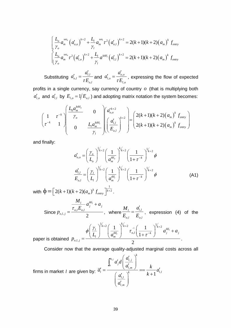
39

( ) ( ) ( )

( ) ( ) ( )

2 22, ,

2 22, ,

2( 1)( 2)

2( 1)( 2)

k ko l

k ol

k k ko lm o o m o l m entry

o l

k k kko lm l o l l m entry

o l

L La a a a k k a f

L La a a a k k a f

θδ θδ

θδ θδ

τγ γ

τγ γ

+ +

+ +

⎧ ′ ′+ = + +⎪⎪⎨⎪ ′ ′+ = + +⎪⎩

Substituting ,,

,

l lo l

o l

aa

Eτ′

′ = and ,,

,

o ol o

l o

aa

Eτ′

′ = , expressing the flow of expected

profits in a single currency, say currency of country o (that is multiplying both

,l oa′ and ,l la′ by , ,1l o o lE E= ) and adopting matrix notation the system becomes:

( )( )

20,

2

,

,

02( 1)( 2)1

1 2( 1)( 2)0

o

l

kkm

o o kkm entryo k

k k kl ll m m entry

o ll

L a ak k a f

aL a k k a f

E

+

−+

−

⎛ ⎞ ′⎛ ⎞⎜ ⎟ ⎛ ⎞⎜ ⎟ + +⎛ ⎞⎜ ⎟ ⎜ ⎟=⎜ ⎟⎛ ⎞′⎜ ⎟⎜ ⎟ ⎜ ⎟⎜ ⎟ + +⎝ ⎠ ⎜ ⎟ ⎝ ⎠⎜ ⎟⎜ ⎟⎜ ⎟⎜ ⎟ ⎝ ⎠⎝ ⎠⎝ ⎠

θδ

θδ

γττ

γ

and finally: 1 12 2 2

,1 1

1o

kk k k

oo o k

o m

aL a

+ + +

−

⎛ ⎞ ⎛ ⎞ ⎛ ⎞′ = ⎜ ⎟ ⎜ ⎟ ⎜ ⎟+⎝ ⎠⎝ ⎠ ⎝ ⎠θδ

γ φτ

1 12 2 2,

,

1 11l

kk k k

l l lk

o l l m

aE L a

+ + +

−

′ ⎛ ⎞ ⎛ ⎞ ⎛ ⎞= ⎜ ⎟ ⎜ ⎟ ⎜ ⎟+⎝ ⎠⎝ ⎠ ⎝ ⎠θδ

γ φτ

(A1)

with 1

22( 1)( 2)( )k km entryk k a f +⎡ ⎤+ +⎣ ⎦φ = .

Since , ,, , 2

llj j

o l o lo l j

M a aE

p

θδ

τ+

= , where ,

, ,

l ll

o l o l

aME E

′= , expression (4) of the

paper is obtained

1

1 12 2 2

,

, ,

1 11

2

l

l

kk k k

lo l j jk

l mo l j

a aL a

p

−+ + +

−

⎛ ⎞ ⎛ ⎞ ⎛ ⎞ +⎜ ⎟ ⎜ ⎟ ⎜ ⎟+⎝ ⎠⎝ ⎠ ⎝ ⎠=

θδθδ

γφ ττ

.

Consider now that the average quality-adjusted marginal costs across all

firms in market l are given by:

, ,

,,

,

,

1

l l

ka l j

jol m

l l lk

l l

l m

aa d

a ka aka

a

′⎛ ⎞′ ⎜ ⎟⎜ ⎟′⎝ ⎠′ ′= ==

+⎛ ⎞′⎜ ⎟⎜ ⎟′⎝ ⎠

∫

40

The average quality-adjusted price level across all varieties sold in country

l , expressed in currency of country l , is ( ), ,1 2 12 2( 1)l

ll l l l l l

l

P kP a a aa kθδ

+′ ′ ′ ′= = + =+

.

Converting lP′ in currency of country o (multiplying by , ,1l o o lE E= ) and

substituting ,

,

l l

o l

aE

′with the expression (A1) one gets equation (5) and may use:

1 12 22

,

1 2( 1)1 2 1

lkk kkl l m

kl o l l

P akL k E a

+ ++

−

⎛ ⎞⎛ ⎞ +⎛ ⎞ ⎜ ⎟=⎜ ⎟ ⎜ ⎟ ⎜ ⎟+ +⎝ ⎠⎝ ⎠ ⎝ ⎠

θδ

γ φτ

to arrive to equation (6) of the main text.

41

REFERENCES

Antoniades A. (2008), Heterogeneous Firms, Quality and Trade, mimeo, Georgetown University.

Atkeson A. and Burstein A. (2008), Pricing-to-Market, Trade Costs and International Relative Prices, mimeo, UCLA University.

Auer R. and Chaney T. (2008), Cost Pass-Through in a Competitive Model of Pricing-to-Market, Swiss National Bank Working Papers, 2008-06.

Baldwin R. (1988), Hysteresis in Import Prices: The Beachhead Effect, American Economic Review 78, pp. 773-785.

Baldwin R. and Harrigan J. (2007), Zeros, Quality and Space: Trade Theory and Trade Evidence, NBER Working Paper Series, 13214.

Berman N., Martin P. and Mayer T. (2009), How Do Different Exporters React to Exchange Rate Changes? Theory, Empirics and Aggregate Implications, CEPR Discussion Paper Series, 7493.

Bernard B. A., Eaton J., Jensen J. B. and Kortum S. (2003), Plants and Productivity in International Trade, American Economic Review 93, pp. 1268-1290.

Bernard B. A., Jensen J. B. (1995), Exporters, Jobs and Wages in US Manufacturing: 1976-87, Brookings Papers on Economic Activity: Microeconomics, 67-112.

Betts C. and Devereux M. (1996), The Exchange Rate in a Model of Pricing to Market, European Economic Review 40, pp. 1007-1021.

Bhat C. R. (2001), Quasi-random Maximum Simulated Likelihood Estimation of the Mixed Multinomial Logit Model, Transportation Research 35, pp. 677-693.

Boes S. and Winkelmann R. (2006) The Effect of Income on Positive and Negative Subjective Well-Being, mimeo, University of Zurich.

Borin A. (2008), Trade and Quality Differentiation among Heterogeneous Firms, mimeo TorVergata University.

Campa, J. M. and Goldberg L. S. (2005) Exchange Rate Pass-through into Import Prices, Review of Economics and Statistics 87, pp. 679-690.

42

Choi, Y. C., Hummels D. and Xiang C. (2009), Explaining Import Quality: The Role of Income Distribution, Journal of International Economics, 77, 265-275.

Corsetti G., Dedola L. and Leduc S. (2005), DSGE Models of High Excnage Rate Volatility and Low Pass-through, Board of Governors Discussion Paper, 845.

Crinò R. and Epifani P. (2008), Productivity and Export Intensity to High-Income and Low-income Countries, mimeo, Bocconi University.

de Nardis S and Pensa C., How Intense is Competition in International Markets of Traditional Goods: The Case of Italian Exporters, Economia internazionale/International Economics, 57, 275-304.

Dornbusch R. (1987), Exchange Rates and Prices, American Economic Review 77, pp. 93-106.

Froot K. A and Klemperer P. D. (1989), Exchange Rate Pass-Through when Markets Share Matters, American Economic Review 79, pp. 637-654.

Goldberg P. K. and Knetter M. M. (1997) Goods Prices and Exchange Rates: What Have We Learned?, Journal of Economic Literature 35, pp. 1243-1272.

Gourieroux C. and A. Monfort (1996), Simulation Based Methods: Econometric Methods, Oxford: Oxford University Press

Greene W. H. (2004), Interpreting Estimated Parameters and Measuring Individual Heterogeneity in Random Coefficient Models, NYU Working Paper, EC-04-08.

Greene, W. H. (2005) Econometric Analysis, New Jersey: Prentice-Hall.

Hallak, J. C. (2006), Product Quality and the Direction of Trade, Journal of International Economics 68, pp. 238-265.

Hummels, D. and Klenow P. (2005), The Variety and Quality of a Nation’s exports, American Economic Review, 95, 704-723.

Hummels, D and Skiba A. (2004), Shipping the Good Apples Out? An Empirical Confirmation of the Alchian-Allen Conjecture, Journal of Political Economy, 112, 1384-1402.

Johnson R. C. (2007), Trade and Prices with Heterogeneous Firms, mimeo, Princeton University.

43

Kasa K. (1992), Adjustment Costs and Pricing to Market, Journal of International Economics 32, pp. 198-210.

Kneller R. and Yu Z. (2008), Quality Selection, Chinese Exports and Theories of Heterogeneous Firm Trade, University of Nottingham Research Paper Series, 2008/44.

Krugman P. R. (1987), Pricing to Market When the Exchange Rate Changes, in S. W. Arndt and J. D. Richardson (eds.). Real Financial Linkages among Open Economies, Cambridge, MA: MIT Press.

Kugler m. and Verhoogen E. (2008), The Quality-Complementarity Hypothesis: Theaory and Evidence from Colombia, NBER Working Paper Series, 13214.

Lissovolick B. (2008), Trends in Italy’s non-price competitiveness, IMF Working Paper, WP/08/124.

Manova K. and Zhang Z. (2009), Export Prices and Heterogeneous Firm Models, NBER Working Paper Series, 15342.

Marston R. C. (1990), Pricing to Market in Japanese Manufacturing, Journal of International Economics 29, pp. 217-236.

McKelvey, R. and Zavonia, W. (1975) A Statistical Model for the Analysis of Ordered Level Dependent Variables, Journal of Mathematical Sociology 4, pp. 103-120.

Melitz M. J and Ottaviano G. I. P. (2008), Market Size, Trade, and Productivity, Review of Economic Studies 75, pp. 295-316.

Train K. (2003), Discrete Choice Methods with Simulation, New York: Cambridge University Press.

Van Praag B. M. S., P. Frijters and A. Ferrer-i-Carbonell (2003), The Anatomy of Subjective Well-Being, Journal of Economic Behavior and Organization 51, pp. 29-49.

Verhoogen E. (2008), Trade, Quality Upgrading and Wage Inequality in the Mexican Manufacturing Sector, Quarterly Journal of Economics, 123, 489-530.

Wooldridge J. (2002), Econometric Analysis of Cross Section and Panel Data, Cambridge, MA: MIT Press.

Working Papers available:

n. 75/07 R. BASILE Intra-distribution dynamics of regional per-capita income in Europe: evidence from alternative conditional density estimators

n. 76/07 M. BOVI National Accounts, Fiscal Rules and Fiscal Policy Mind the Hidden Gaps

n. 77/07 L. CROSILLA S. LEPROUX

Leading indicators on construction and retail trade sectors based on ISAE survey data

n. 78/07 R. CERQUETI M. COSTANTINI

Non parametric Fractional Cointegration Analysis

n. 79/07 R. DE SANTIS C. VICARELLI

The “deeper” and the “wider” EU strategies of trade integration

n. 80/07 S. de NARDIS R. DE SANTIS C. VICARELLI

The Euro’s Effects on Trade in a Dynamic Setting

n. 81/07 M. BOVI R. DELL’ANNO

The Changing Nature of the OECD Shadow Economy

n. 82/07 C. DE LUCIA Did the FED Inflate a Housing Price Bubble? A Cointegration Analysis between the 1980s and the 1990s

n. 83/07 T. CESARONI Inspecting the cyclical properties of the Italian Manufacturing Business survey data

n. 84/07 M. MALGARINI Inventories and business cycle volatility: an analysis based on ISAE survey data

n. 85/07 D. MARCHESI The Rule Incentives that Rule Civil Justice

n. 86/07 M. COSTANTINI S. de NARDIS

Estimates of Structural Changes in the Wage Equation: Some Evidence for Italy

n. 87/07 R. BASILE M. MANTUANO

La concentrazione geografica dell’industria in Italia: 1971-2001

n. 88/07 S. de NARDIS R. DE SANTIS C. VICARELLI

The single currency’s effects on Eurozone sectoral trade: winners and losers?

n. 89/07 B.M. MARTELLI G. ROCCHETTII

Cyclical features of the ISAE business services series

Working Papers available:

n. 90/08 M. MALGARINI Quantitative inflation perceptions and expectations of Italian Consumers

n. 91/08 P. L. SCANDIZZO M. VENTURA

Contingent valuation of natural resources:

a case study for Sicily

n. 92/08 F. FULLONE B.M. MARTELLI

Re-thinking the ISAE Consumer Survey Processing Procedure

n. 93/08 M. BOVI P. CLAEYS

Treasury v dodgers. A tale of fiscal consolidation and tax evasion

n. 94/08 R. DI BIASE Aliquote di imposta sul lavoro dipendente:

analisi per figure tipo e con dati campionari

n. 95/08 M. BOVI The “Psycho-analysis” of Common People’s Forecast Errors. Evidence from European Consumer Surveys

n. 96/08 F. BUSATO A. GIRARDI A. ARGENTIERO

Technology and non-technology shocks in a two-sector economy

n. 97/08 A. GIRARDI The Informational Content of Trades on the EuroMTS Platform

n. 98/08 G. BRUNO Forecasting Using Functional Coefficients Autoregressive Models

n. 99/08 A. MAJOCCHI A. ZATTI

Land Use, Congestion and Urban Management

n. 100/08 A. MAJOCCHI Theories of Fiscal Federalism and the European Experience

n. 101/08 S. de NARDIS C. PAPPALARDO C. VICARELLI

The Euro adoption’s impact on extensive and intensive margins of trade: the Italian case

n. 102/08 A. GIRARDI P.PAESANI

Structural Reforms and Fiscal Discipline in Europe

n. 103/08 S. TENAGLIA M. VENTURA

Valuing environmental patents legal protection when data is not availableby

n. 104/08 P. L. SCANDIZZO M. VENTURA

A model of public and private partnership through concession contracts

Working Papers available:

n. 105/08 M. BOSCHI A. GIRARDI

The contribution of domestic, regional and international factors to Latin America’s business cycle

n. 106/08 T. CESARONI

Economic integration and industrial sector fluctuations: evidence from Italy

n. 107/08 G. BOTTONE

Human Capital: an Institutional Economics point of view

n. 108/09 T. CESARONI M. MALGARINI L. MACCINI

Business cycle stylized facts and inventory behaviour: new evidence for the Euro area

n. 109/09 G. BOTTONE

Education in Italy: is there any return?

n. 110/09 S. de NARDIS C. PAPPALARDO

Export, Productivity and Product Switching: the case of Italian Manufacturing Firms

n. 111/09 M. BOVI R. CERQUETI

Why is the Tax Evasion so Persistent?

n. 112/09 B. ANASTASIA M. MANCINI U. TRIVELLATO

Il sostegno al reddito dei disoccupati: note sullo stato dell’arte. Tra riformismo strisciante,inerzie dell’impianto categoriale e incerti orizzonti di flexicurity

n. 113/09 A. ARGENTIERO Some New Evidence on the Role of Collateral: Lazy Banks or Diligent Banks?

n. 114/09 M. FIORAMANTI Estimation and Decomposition of Total Factor Productivity Growth in the EU Manufacturing Sector: a Stochastic Frontier Approach

n. 115/09 E. DE ANGELIS C. PAPPALARDO

String Matching Algorithms. An Application to ISAE and ISTAT Firms’ Registers

n. 116/09 L. CROSILLA S. LEPROUX M. MALGARINI F. SPINELLI

Factor based Composite Indicators for the Italian Economy

n. 117/09 G. BOTTONE A new notion of progress: Institutional quality

Working Papers available:

n. 118/09 F. DI NICOLA Tassazione e Sostegno del Reddito Familiare

n. 119/09 G. BRUNO Non-linear relation between industrial production and business surveys data

n. 120/09 R. CERQUETI M. VENTURA

A Discrete Model for Patent Valuation

n. 121/09 M. MALGARINI M. PUGNO G. ZEZZA

Life Satisfaction in Italy: Evidence from the ISAE Consumers Survey

n. 122/09 R. BASILE A. GIRARDI

Specialization and Risk Sharing: evidence from European Regions