Issues in the Development of Global Optimization Algorithms

for Bilevel Programs with a Nonconvex Inner Program

Alexander Mitsos and Paul I. Barton*

Department of Chemical Engineering

Massachusetts Institute of Technology,

66-464, 77 Massachusetts Avenue

Cambridge, MA 02139

mitsos@mit.edu and pib@mit.edu

tel: 617-253-6526, fax: 617-258-5042

February 13, 2006

Updated: October 16, 2006

Abstract

The co-operative formulation of a nonlinear bilevel program involving nonconvex functions is considered

and two equivalent reformulations to simpler programs are presented. It is shown that previous literature

proposals for the global solution of such programs are not generally valid for nonconvex inner programs

and several consequences of nonconvexity in the inner program are identified. In particular, issues with the

computation of lower and upper bounds as well as with the choice of branching variables in a branch-and-

bound framework are analyzed. This analysis lays the foundation for the development of rigorous algorithms

and some algorithmic expectations are established.

Key-words

Bilevel program; nonconvex; global optimization; GSIP; branch-and-bound

AMS Classification

http://www.ams.org/msc/

65K05=mathematical programming algorithms

90C26=nonconvex programming

90c33=complementarity programming

90C31=sensitivity,stability,parametric optimization

1

1 Introduction

Bilevel optimization has applications in a variety of economic and engineering problems and several optimiza-

tion formulations can be transformed to bilevel programs. There are many contributions in the literature and

the reader is directed to other publications for a review of applications and algorithms [10, 24, 4, 14, 26, 17, 18].

Here, inequality constrained nonlinear bilevel programs of the form

minx,y

f(x,y)

s.t. g(x,y) ≤ 0

y ∈ arg minz

h(x, z) (1)

s.t. p(x, z) ≤ 0

x ∈ X y, z ∈ Y,

are considered. The co-operative (optimistic) formulation [14] is assumed, where if for a given x the inner

program has multiple optimal solutions y, the outer optimizer can choose among them. As has been proposed

in the past, e.g., [11, 2], dummy variables (z instead of y) are used in the inner program since this clarifies

some issues and facilitates discussion. A minimal assumption for an algorithmic development based on

branch-and-bound (B&B) is compact host sets X ⊂ Rnx , Y ⊂ R

ny and continuous functions f : X×Y → R,

g : X × Y → Rng , h : X × Y → R and p : X × Y → R

np . For some of the methods discussed here further

assumptions, such as twice continuously differentiable functions or constraint qualifications, are needed. Note

that equality constraints have only been omitted for the sake of simplicity and would not alter anything in

the discussion of this paper.

2

For a fixed x we denote

minz

h(x, z)

s.t. p(x, z) ≤ 0 (2)

z ∈ Y,

the inner program. The parametric optimal solution value of this program is denoted w(x) and the set of

optimal points H(x). We focus on nonconvex inner programs, i.e., the case when some of the functions

p(x, z), h(x, z) are not partially convex with respect to z for all possible values of x.

Most of the literature is devoted to special cases of (1), in particular linear functions, e.g., [9]. Typically,

the inner program is assumed convex satisfying a constraint qualification and is replaced by the equivalent

KKT first-order optimality conditions; the resulting single level mathematical program with equilibrium

constraints (MPEC) violates the Mangasarian-Fromovitz constraint qualification due to the complementar-

ity slackness constraints [29]. Fortuny-Amat and McCarl [15] reformulate the complementarity slackness

conditions using integer variables. Stein and Still [29] consider generalized semi-infinite programs (GSIP)

and use a regularization of the complementarity slackness constraints. We will discuss how this strategy

could be adapted to general bilevel programs (1).

Very few proposals have been made for bilevel programs with nonconvex functions. Clark and Westerberg

[12] introduced the notion of a local solution where the inner and outer programs are solved to local optimality.

Gumus and Floudas [17] proposed a B&B procedure to obtain the global solution of bilevel programs; we

will show here that this procedure is not valid in general when the inner program (2) is nonconvex. For the

case of GSIP an algorithm based on B&B and interval extensions has been recently proposed by Lemonidis

and Barton [20].

We first discuss what is a reasonable expectation for the solution of nonconvex bilevel programs based

on state-of-the-art notions in global optimization. To analyze some of the consequences of nonconvexity in

the inner program we first introduce two equivalent reformulations of (1) as a simpler bilevel program and

3

as a GSIP. We then discuss how to treat the inner variables in a B&B framework and identify issues with

literature proposals regarding lower and upper bounds. Finally for KKT based approaches we discuss the

need for bounds on the KKT multipliers.

2 Optimality Requirement

An interesting question is how exactly to interpret the requirement y ∈ arg minz∈Y,p(x,z)≤0 h(x, z) which

by definition means that any feasible y is a global minimum of the inner program for a fixed value of x.

Clark and Westerberg [12] proposed the notion of local solutions to the bilevel program (1) requiring that a

furnished solution pair (x, y) satisfies local optimality in the inner program. This is in general a very strong

relaxation.

Note though that in single-level optimization finitely terminating algorithms guaranteeing global opti-

mality exist only for special cases, e.g., linear programs. For nonconvex nonlinear programs (NLP)

f∗ = minx

f(x)

s.t. g(x) ≤ 0 (3)

x ∈ X

state-of-the-art algorithms in general only terminate finitely with an εf -optimal solution. That is, given any

εf > 0 a feasible point x is furnished and a guarantee that its objective value is not more than εf larger

than the optimal objective value

f(x) ≤ f∗ + εf .

Moreover, to our best knowledge, no algorithm can provide guarantees for the distance of the points furnished

from optimal solutions (||x − x∗||, where x∗ is some optimal solution), which would allow a direct estimate

of the requirement y ∈ arg min. Finally global and local solvers for (3) typically allow an εg violation of the

constraints [25].

4

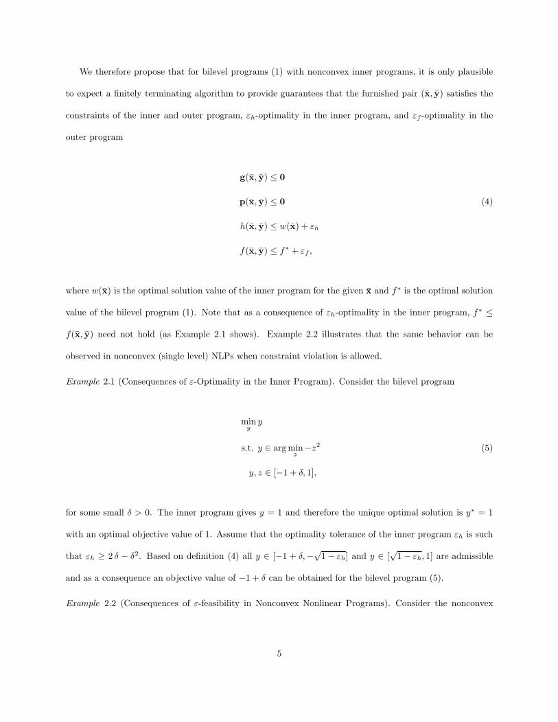
We therefore propose that for bilevel programs (1) with nonconvex inner programs, it is only plausible

to expect a finitely terminating algorithm to provide guarantees that the furnished pair (x, y) satisfies the

constraints of the inner and outer program, εh-optimality in the inner program, and εf -optimality in the

outer program

g(x, y) ≤ 0

p(x, y) ≤ 0 (4)

h(x, y) ≤ w(x) + εh

f(x, y) ≤ f∗ + εf ,

where w(x) is the optimal solution value of the inner program for the given x and f∗ is the optimal solution

value of the bilevel program (1). Note that as a consequence of εh-optimality in the inner program, f∗ ≤

f(x, y) need not hold (as Example 2.1 shows). Example 2.2 illustrates that the same behavior can be

observed in nonconvex (single level) NLPs when constraint violation is allowed.

Example 2.1 (Consequences of ε-Optimality in the Inner Program). Consider the bilevel program

miny

y

s.t. y ∈ arg minz

−z2 (5)

y, z ∈ [−1 + δ, 1],

for some small δ > 0. The inner program gives y = 1 and therefore the unique optimal solution is y∗ = 1

with an optimal objective value of 1. Assume that the optimality tolerance of the inner program εh is such

that εh ≥ 2 δ − δ2. Based on definition (4) all y ∈ [−1 + δ,−√1 − εh] and y ∈ [

√1 − εh, 1] are admissible

and as a consequence an objective value of −1 + δ can be obtained for the bilevel program (5).

Example 2.2 (Consequences of ε-feasibility in Nonconvex Nonlinear Programs). Consider the nonconvex

5

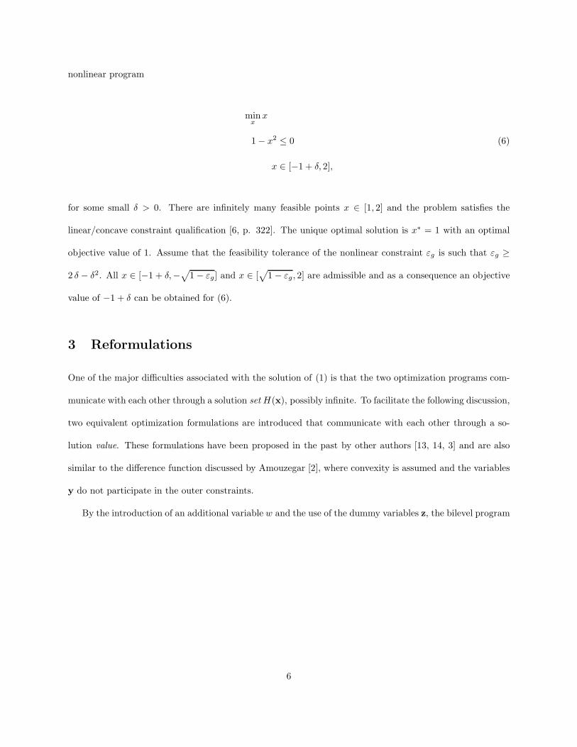
nonlinear program

minx

x

1 − x2 ≤ 0 (6)

x ∈ [−1 + δ, 2],

for some small δ > 0. There are infinitely many feasible points x ∈ [1, 2] and the problem satisfies the

linear/concave constraint qualification [6, p. 322]. The unique optimal solution is x∗ = 1 with an optimal

objective value of 1. Assume that the feasibility tolerance of the nonlinear constraint εg is such that εg ≥

2 δ − δ2. All x ∈ [−1 + δ,−√

1 − εg] and x ∈ [√

1 − εg, 2] are admissible and as a consequence an objective

value of −1 + δ can be obtained for (6).

3 Reformulations

One of the major difficulties associated with the solution of (1) is that the two optimization programs com-

municate with each other through a solution set H(x), possibly infinite. To facilitate the following discussion,

two equivalent optimization formulations are introduced that communicate with each other through a so-

lution value. These formulations have been proposed in the past by other authors [13, 14, 3] and are also

similar to the difference function discussed by Amouzegar [2], where convexity is assumed and the variables

y do not participate in the outer constraints.

By the introduction of an additional variable w and the use of the dummy variables z, the bilevel program

6

(1) is equivalent [13, 14] to

minx,y,w

f(x,y)

s.t. g(x,y) ≤ 0

p(x,y) ≤ 0

h(x,y) − w ≤ 0 (7)

x ∈ X y ∈ Y w ∈ R

w = minz

h(x, z)

s.t. p(x, z) ≤ 0

z ∈ Y.

What is achieved with the introduction of the extra variable w is that the outer and inner program are

coupled by a much simpler requirement, namely the optimal solution value of an optimization program

(min) as opposed to the set of optimal solutions (arg min).

In principle (7) could be solved using multi-parametric optimization as a subproblem. As a first step a

global multi-parametric optimization algorithm would be used for the solution of the inner program for all

x ∈ X dividing X into regions where the minimum w(x) is a known (smooth) function. The second step

would be a global solution of the outer program for each of the optimality regions. This procedure is not

suggested as a solution strategy since it would be overly computationally intensive. Note that application of

this solution strategy to the original bilevel program (1) would require a parametric optimization algorithm

that furnishes all optimal solutions as a function of the parameter x, and to our best knowledge this is not

possible at present.

The simplified bilevel program (7) allows the following observation: a relaxation of the inner program

results in a restriction of the overall program and vice-versa. This observation also holds for other programs

with a bilevel interpretation such as GSIPs, see [21], but does not hold for the original bilevel program

7

(1) because any alteration of the inner program can result in an alteration of its set of optimal solutions

and as such to the formulation of an unrelated optimization problem. We will show though that since

relaxing the inner program in (7) results in an underestimation of w, the constraint h(x,y)−w ≤ 0 becomes

infeasible. Indeed, consider any x and the corresponding optimal objective value of the inner program (2)

w. By the definition of optimality we have h(x,y) ≥ w for all y feasible in the inner program, i.e., ∀y ∈ Y ,

s.t. p(x,y) ≤ 0. As a consequence no y exists that can satisfy all the constraints of (7) exactly if w is

underestimated. If εh optimality of the inner program is acceptable and the magnitude of the underestimation

is less than εh it is possible to obtain (approximately) feasible points of (7).

The bilevel programs (1) and (7) are also equivalent to the following GSIP [3]

minx,y

f(x,y)

s.t. g(x,y) ≤ 0

p(x,y) ≤ 0 (8)

x ∈ X y ∈ Y

h(x,y) ≤ h(x, z), ∀z ∈ Y (x)

Y (x) = {z ∈ Y : p(x, z) ≤ 0}.

Note that this reformulation does not contradict the observation by Stein and Still [28] that under certain

assumptions GSIP problems can be viewed as a special case of bilevel programs. Stein and Still compare a

GSIP with variables x to a bilevel program with variables x and y whereas the bilevel considered here (1)

and the GSIP (8) have the same set of variables x,y. Moreover, the GSIP (8) does not necessarily satisfy

the assumptions made by Stein and Still [28]. Note also that the GSIP (8) does not contain any Slater points

as defined in Lemonidis and Barton [21] unless εh optimality of the inner program is allowed.

In either of the two reformulated programs our proposal of εh optimality can be interpreted as εh feasibility

of the coupling constraint. As mentioned above, NLP solvers typically allow such a violation of ordinary

nonlinear constraints, and this motivates again the proposal of ε-optimality (4).

8

4 Branching on the y Variables

As mentioned in the introduction, the main focus of this publication is on the consequences of nonconvex

inner programs for B&B procedures. In this section we briefly review some features of this algorithm class

and discuss complications for the inner variables. For more details on B&B procedures the reader is referred

to the literature, e.g., [19, 30]. For discussion purposes consider again the inequality constrained nonconvex

nonlinear program (NLP) (3). The goal of B&B is to bracket the optimal solution value f∗ between an upper

bound UBD, typically the objective value at a feasible point, and a lower bound LBD, typically the optimal

objective value of a relaxed program. To that end the host set X is partitioned into a finite collection of

subsets Xi ⊂ X , such that X = ∪iXi. For each subset i a lower bound LBDi and an upper bound UBDi are

established. The partitions are successively refined and typically this is done in an exhaustive matter [19], i.e.,

the diameter of each subset tends to zero. At each iteration the bounds are updated LBD = mini LBDi and

UBD = mini UBDi. Therefore UBD is non-increasing and LBD non-decreasing. The algorithm terminates

when the difference UBD − LBD is lower than a pre-specified tolerance.

For bilevel programs the inner program can have multiple optimal solutions for some values of x and

therefore a complication is whether or not to branch on the variables y. Gumus and Floudas [17] do not

specify in their proposal if they do, and all their examples are solved at the root node. Amouzegar [2] for a

special convex case proposes to only branch on the variables x.

The dilemma is that on one hand y are optimization variables in the outer program which suggests

that one should branch on them but on the other hand the requirement of optimality in the inner program

requires consideration of the whole set Y without branching. One extreme possibility is to branch on the

variables x ∈ X and y ∈ Y without distinction. Example 4.1 shows that some points (x, y) ∈ Xi × Yi could

be feasible for node i but not for the original program (1) and therefore UBD = mini UBDi cannot be used.

The other extreme possibility is to consider for a given node Xi a partition of Y to subsets Yj and keeping

the worst subset. This procedure is not correct either as Example 4.2 shows. The introduction of dummy

variables z for the inner program allows the distinction of y between the inner and the outer programs. In

a forthcoming publication [23] we propose an algorithm where branching is performed on the y variables,

9

but not on the z variables. An alternative would be to employ subdivision similar to ideas presented for

Semi-Infinite Programs [7, 8].

Example 4.1 (The host set of the inner program cannot be partitioned). Consider the simple linear bilevel

program

miny

y

s.t. − y ≤ 0 (9)

y ∈ argminz

z

y, z ∈ [−1, 1].

The inner program gives y = −1 which is infeasible in the outer program by the constraint y ≥ 0. If we

partition the host set Y = [−1, 1] by bisection (Y1 = [−1, 0] and Y2 = [0, 1]) we obtain two bilevel programs.

The first one

miny

y

s.t. − y ≤ 0

y ∈ argminz

z

y, z ∈ [−1, 0]

is also infeasible by the same argument. The second

miny

y

s.t. − y ≤ 0

y ∈ argminz

z

y, z ∈ [0, 1]

10

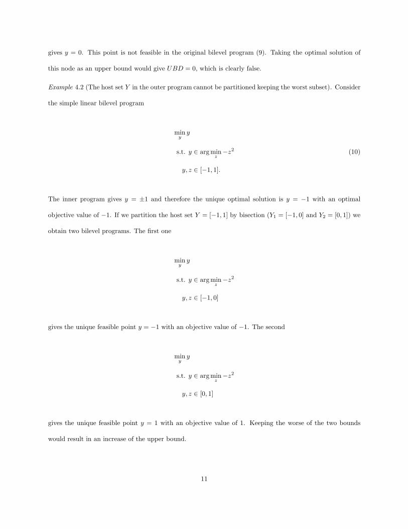
gives y = 0. This point is not feasible in the original bilevel program (9). Taking the optimal solution of

this node as an upper bound would give UBD = 0, which is clearly false.

Example 4.2 (The host set Y in the outer program cannot be partitioned keeping the worst subset). Consider

the simple linear bilevel program

miny

y

s.t. y ∈ argminz

−z2 (10)

y, z ∈ [−1, 1].

The inner program gives y = ±1 and therefore the unique optimal solution is y = −1 with an optimal

objective value of −1. If we partition the host set Y = [−1, 1] by bisection (Y1 = [−1, 0] and Y2 = [0, 1]) we

obtain two bilevel programs. The first one

miny

y

s.t. y ∈ argminz

−z2

y, z ∈ [−1, 0]

gives the unique feasible point y = −1 with an objective value of −1. The second

miny

y

s.t. y ∈ argminz

−z2

y, z ∈ [0, 1]

gives the unique feasible point y = 1 with an objective value of 1. Keeping the worse of the two bounds

would result in an increase of the upper bound.

11

5 Upper Bounding Procedure

Obtaining upper bounds for bilevel programs with a nonconvex inner program is very difficult due to the

constraint “y is a global minimum of the inner program” and no obvious restriction of this constraint is

available. Applying this definition to check the feasibility of a pair of candidate solutions (x, y) results in a

global optimization problem for which in general state-of-the-art algorithms only furnish εf -optimal solutions

at finite termination.

Only recently cheap upper bounds have been developed for some related problems such as SIPs [7, 8]

and GSIPs [21] under nonconvexity. In these proposals the upper bounds are associated only with a feasible

point x and no identification of the inner variables is needed. Cheap upper bounds are conceivable for a

general bilevel program but to our best knowledge no valid proposal exists for the case of nonconvex inner

programs. On termination, algorithms for bilevel programs (1) have to furnish a feasible pair (x, y), i.e.,

values must be given for the inner variables. If the upper bounds obtained in a B&B tree are associated

with such feasible points, a global solution to a nonconvex optimization program has to be identified for

each upper bound. This leads to an exponential procedure nested inside an exponential procedure and is

being employed in a forthcoming publication [23]. To avoid the nested exponential procedure a formulation

of upper bounds without the identification of feasible points is required.

5.1 Solving a MPEC Locally Does Not Produce Valid Upper Bounds

Gumus and Floudas [17] propose to obtain an upper bound by replacing the inner program by the corre-

sponding KKT conditions, under some constraint qualification, and then solving the resulting program to

local optimality. In this section it is shown that this procedure does not in general generate valid upper

bounds. In the case of a nonconvex inner program, the KKT conditions are not sufficient for a global min-

imum and replacing the inner (nonconvex) program by the (necessary only) KKT conditions amounts to a

relaxation of the bilevel program. Solving a (nonconvex) relaxed program to local optimality provides no

guarantees that the point found is feasible to the original bilevel program; moreover the objective value does

not necessarily provide an upper bound on the original bilevel program. This behavior is shown in Example

12

5.1. Although this example has a special structure, it shows a general property. Moreover in the proposal

by Gumus and Floudas [17] the complementarity constraint is replaced by the big-M reformulation and new

variables are introduced; some issues associated with this are discussed in Section 7.

Example 5.1 (Counterexample for upper bound based on local solution of MPEC). For simplicity a bilevel

program with a single variable y and box constraints is considered.

miny

y

s.t. y ∈ argminz

−z2 (11)

y, z ∈ [−0.5, 1].

By inspection the solution to the bilevel program (11) is y = 1 with an optimal objective value 1. The inner

program has a concave objective function and linear inequality constraints and therefore by the Adabie

constraint qualification the KKT conditions are necessary [5, p. 187]. The KKT conditions for the inner

program are given by

−0.5 − y ≤ 0

y − 1 ≤ 0

−2 y − λ1 + λ2 = 0

λ1 (−y − 0.5) = 0 (12)

λ2 (y − 1) = 0

λ1 ≥ 0

λ2 ≥ 0.

System (12) has three solutions. The first solution is y = −0.5, λ1 = 1, λ2 = 0, a suboptimal local minimum

of the inner program (h = −0.25). The second solution is y = 0, λ1 = 0, λ2 = 0, the global maximum of the

13

inner program (h = 0). Finally the third solution is y = 1, λ1 = 0, λ2 = 2, the global minimum of the inner

program (h = −1). The one-level optimization program proposed by Gumus and Floudas [17] is therefore

equivalent to

miny

y

s.t. y ∈ {−0.5, 0, 1} (13)

and has three feasible points. Since the feasible set is discrete, all points are local minima and a local solver

can converge to any of the points corresponding to the solutions of the system (12). The first solution

y = −0.5, with an objective value f = −0.5 and the second solution y = 0, with an objective value f = 0 are

both infeasible for (11). Moreover they clearly do not provide valid upper bounds on the original program

(11). The third solution y = 1 with an objective value of f = 1, which has the worst objective value for (13),

is the true solution to the original program (11). Note that solving (13) to global optimality would provide

a valid lower bound as described in the next section.

6 Lower Bounding Procedure

Lower bounds are typically obtained with an underestimation of the objective function and/or a relaxation

of the feasible set [19] and a global solution of the resulting program. While global solution is a necessary

requirement to obtain a valid lower bound, typically the constructed programs are convex and therefore

global optimality can be guaranteed with local solvers.

6.1 Relaxation of the Inner Program Does Not Provide a Valid Lower Bound

Gumus and Floudas [17] propose to obtain a lower bound to the bilevel program (1) by constructing a convex

relaxation of the inner program (2) and replacing the convex inner program by its KKT conditions. Consider

14

for a fixed x a convex relaxation of (2) and the corresponding set of optimal solutions Hc(x)

Hc(x) =arg minz

hc(x, z)

s.t. pc(x, z) ≤ 0 (14)

z ∈ Y,

where hc(x, ·) and pc(x, ·) are convex underestimating functions of h(x, ·) and p(x, ·) on Y for fixed x. This

procedure results in an underestimation of the optimal solution value of the inner program but typically not

in a relaxation of the feasible set of the bilevel program (1). The desired set inclusion property for the two

sets of optimal solutions

H(x) ⊂ Hc(x) (15)

does not hold in general. It does hold when the inner constraints p(x, ·) are convex and hc(x, ·) is the convex

envelope of h(x, ·). Constructing the convex envelope is in general not practical and Gumus and Floudas

propose to use α-BB relaxations [1]. Example 6.1 shows that convex underestimating functions based on

this method do not guarantee the desired set inclusion property even in the case of linear constraints. In the

case of nonconvex constraints one might postulate that the set inclusion property (15) holds if the feasible

set is replaced by its convex hull and the objective function by the convex envelope. This is not true, as

shown in Example 6.2. Both examples show that the proposal by Gumus and Floudas does not provide

valid lower bounds for bilevel programs involving a nonconvex inner program. Although the examples have

a special structure, they show a general property. Moreover in the proposal by Gumus and Floudas [17] the

complementarity constraint is replaced by the big-M reformulation and new variables are introduced; issues

associated with this are discussed in Section 7.

Example 6.1 (Counterexample for lower bound based on relaxation of inner program: box constraints). For

15

simplicity a bilevel program with a single variable y and box constraints is considered.

miny

y

s.t. y ∈ arg minz

z3 (16)

y, z ∈ [−1, 1].

The inner objective function is monotone and the unique minimum of the inner program is y∗ = −1. The

bilevel program is therefore equivalent to

miny

y

s.t. y = −1

y ∈ [−1, 1]

with the unique feasible point y∗ = −1 and an optimal objective value of −1. Taking the α-BB relaxation

for α = 3 (the minimal possible) of the inner objective function, the relaxed inner program is

minz

z3 + 3(1 − z)(−1 − z)

s.t. z ∈ [−1, 1],

which has the unique solution y∗ = 0, see also Figure 1. Clearly the desired set inclusion property (15)

is violated. Using the solution to the convex relaxation of the inner program, the bilevel program now is

equivalent to

miny

y

s.t. y = 0

y ∈ [−1, 1]

16

and a false lower bound of 0 is obtained. Note that since the objective function is a monomial, its convex

envelope is known [22]

hc(z) =

3/4z − 1/4 if z ≤ 1/2

z3 otherwise.

By replacing the inner objective with the convex envelope the minimum of the relaxed inner program would

be attained at y∗ = −1 and the set inclusion property would hold.

−4

−3

−2

−1

0

1

−1 −0.5 0 0.5 1

convex envelope

original function

α-BB underestimator

z

Figure 1: Inner level objective function, its convex envelope and its α-BB underestimator for example (6.1)

Example 6.2 (Counterexample for lower bound based on relaxation of inner program: nonconvex constraints).

For simplicity a bilevel program with a single variable y convex objective functions and a single nonconvex

constraint in the inner program is considered.

miny

y

s.t. y ∈ argminz

z2 (17)

s.t. 1 − z2 ≤ 0

y, z ∈ [−10, 10].

17

The two optimal solutions of the inner program are y∗ = ±1, so that the bilevel program becomes

miny

y

s.t. y = ±1

y ∈ [−10, 10]

with the unique optimal point y∗ = −1 and an optimal objective value of −1. Taking the convex hull of the

feasible set in the inner program, the relaxed inner program

minz

z2

s.t. z ∈ [−10, 10]

has the unique solution y∗ = 0. Clearly the desired set inclusion property (15) is violated. Using the solution

to the convex relaxation of the inner program, the bilevel program program becomes

miny

y

s.t. y = 0

y ∈ [−10, 10].

and a false lower bound of 0 is obtained. Note that using any valid underestimator for the function 1 − z2

would result in the same behavior as taking the convex hull.

6.2 Lower Bounds Based on Relaxation of Optimality Constraint

A conceptually simple way of obtaining lower bounds to the bilevel programs is to relax the constraint “y

is a global minimum of the inner program” with the constraint “y is feasible in the inner program” and

to solve the resulting program globally. Assuming some constraint qualification, a tighter bound can be

18

obtained by the constraint “y is a KKT point of the inner program”. In a forthcoming publication [23]

we analyze how either relaxation can lead to convergent lower bounds. As mentioned in the introduction,

Stein and Still [29] propose to solve GSIPs with a convex inner program by solving regularized MPECs.

They note that for nonconvex inner programs this strategy would result to a relaxation of the GSIP. The

complementarity slackness condition µigi(x, z) = 0 is essentially replaced by µigi(x, z) = −τ2, where τ is

a regularization parameter. A sequence τ → 0 of regularized programs is solved; each of the programs is a

relaxation due to the special structure of GSIPs. For a general bilevel program the regularization has to be

slightly altered as can be seen in Example 6.3. The complication is that the KKT points are not feasible

points in the regularized program and only for τ → 0 would a solution to the MPEC program provide

a lower bound to the original bilevel program. A possibility to use the regularization approach for lower

bounds would be to use an inequality constraint −τ2 ≤ µigi(x, z) as in [27]. To obtain the global solution

with a branch-and-bound algorithm an additional complication is upper bounds for the KKT multipliers,

see Section 7.

Example 6.3 (Example for complication in lower bound based on regularized MPEC). Consider a linear

bilevel program with a single variable y and for simplicity take R as the host set.

miny

y

s.t. y ∈ arg minz

z (18)

s.t. − z ≤ 0

y, z ∈ R.

The inner program has the unique solution y = 0, and thus there is only one feasible point in the bilevel

program with an objective value of 0. Note that all the functions are affine, and the inner program satisfies

19

a constraint qualification. The equivalent MPEC is

miny

y

s.t. 1 − µ = 0

µ ≥ 0

−y ≤ 0

µ (−y) = 0

y ∈ R.

From the stationarity condition 1−µ = 0 it follows µ = 1 and therefore from the complementarity slackness

y = 0. As explained by Stein and Still [29] the regularized MPEC is equivalent to the solution of

miny

y

s.t. 1 − µ = 0

µ ≥ 0 (19)

−y ≤ 0

µ (−y) = −τ2

y ∈ R,

which gives µ = 1, y = τ2 and an objective value of τ2, which clearly is not a lower bound to 0. Replacing

the requirement µy = 0 by −τ2 ≤ µ(−y) or equivalently y ≤ τ2/µ in (19) would give a correct lower bound

of 0.

20

7 Complication in KKT Approaches: Bounds

A complication with bounds based on KKT conditions are that extra variables µ (KKT multipliers) are

introduced (one for each constraint) which are bounded only below (by zero). The big-M reformulation

of the complementarity slackness condition needs explicit bounds for both the constraints gi and KKT

multipliers µi. Fortuny-Amat and McCarl [15] first proposed the big M-reformulation but do not specify

how big M should be. Gumus and Floudas [17] use the upper bound on slack variables as an upper bound

for the KKT multipliers which is not correct in general as Example 7.1 shows. Note also that Gumus and

Floudas [17] do not specify how to obtain bounds on the slack variables of the constraints but this can be

easily done, e.g., by computing an interval extension of the inequality constraints. Moreover, for a valid

lower bound a further relaxation or a global solution of the relaxations constructed is needed and typically

all variables need to be bounded [30, 25]. The regularization approach as in Stein and Still [29] does not need

bounds for the regularization but if the resulting program is to be solved to global optimality bounds on the

KKT multipliers are again needed. For programs with a special structure upper bounds may be known a

priori or it may be easy to estimate those. Examples are the feasibility test and flexibility index problems

[16] where all KKT multipliers are bounded above by 1. Alternatively, specialized algorithms need to be

employed that do not require bounds on the KKT multipliers.

Example 7.1 (Example with arbitrarily large KKT multipliers). Let us now consider a simple example with

a badly scaled constraint that leads to arbitrarily large multipliers for the optimal KKT point

minz

−z

δ(z2 − 1) ≤ 0 (20)

z ∈ [−2, 2],

where δ > 0. The only KKT point and optimal solution point is z = 1 and the KKT multiplier associated

with the constraint δ(z2−1) ≤ 0 is µ = 12δ

. The slack variable associated with the constraint can at most take

the value −δ. As δ → 0, the gradient of the constraint at the optimal solution d(δ(z2−1))dz

= 2 δ ζ = 2 δ → 0

21

and µ becomes arbitrarily large. For δ = 0 the Slater constraint qualification is violated.

8 Conclusions

The bilevel program involving nonconvex functions has been discussed, with emphasis on the solution of

programs involving nonconvexity in the inner program within a branch-and-bound framework. To that

extent two equivalent reformulations of the bilevel program as a simpler bilevel program and as a GSIP have

been presented. As a compromise between local and global solution of the inner program, solution to ε-

optimality in the inner and outer programs has been proposed. Several consequences of nonconvexity in the

inner program have been identified, and the validity of literature proposals has been explored theoretically

and through simple illustrative examples. In particular, it was shown that replacing the inner program by its

necessary but not sufficient KKT constraints and solving the resulting MPEC locally does not produce valid

upper bounds. Similarly, a relaxation of the inner program does not lead to a valid lower bound whereas

a relaxation of the optimality constraint does. In the co-operative formulation the inner variables have to

be treated differently than the outer variables. For KKT based approaches, bounds on the KKT multipliers

are needed for a global solution of the formulated subproblems. The issues identified with current proposals

available in the literature show the need for the development of a rigorous algorithm for the global solution

of bilevel programs involving nonconvex functions in the inner program.

Acknowledgments

This work was supported by the DoD Multidisciplinary University Research Initiative (MURI) program

administered by the Army Research Office under Grant DAAD19-01-1-0566.

We would like to thank Binita Bhattacharjee, Panayiotis Lemonidis, Benoıt Chachuat, Ajay Selot and Cha

Kun Lee for fruitful discussions.

22

References

[1] Claire S. Adjiman and Christodoulos A. Floudas. Rigorous convex underestimators for general twice-

differentiable problems. Journal of Global Optimization, 9(1):23–40, 1996.

[2] Mahyar A. Amouzegar. A global optimization method for nonlinear bilevel programs. IEEE Transactions

on Systems, Man and Cybernetics–Part B: Cybernetics, 29(6):771–777, 1999.

[3] Jonathan F. Bard. An algorithm for solving the general bilevel programming problem. Mathematics of

Operations Research, 8(2):260–272, 1983.

[4] Jonathan F. Bard. Practical Bilevel Optimization: Algorithms and Applications. Nonconvex Optimiza-

tion and Its Applications. Kluwer Academic Publishers, Dordrecht, 1998.

[5] Mokhtar S. Bazaraa, Hanif D. Sherali, and C. M. Shetty. Nonlinear Programming. John Wiley & Sons,

New York, Second edition, 1993.

[6] Dimitri P. Bertsekas. Nonlinear Programming. Athena Scientific, Belmont, Massachusetts, Second

edition, 1999.

[7] Binita Bhattacharjee, William H. Green Jr., and Paul I. Barton. Interval methods for semi-infinite

programs. Computational Optimization and Applications, 30(1):63–93, 2005.

[8] Binita Bhattacharjee, Panayiotis Lemonidis, William H. Green Jr., and Paul I. Barton. Global solution

of semi-infinite programs. Mathematical Programming, Series B, 103(2):283–307, 2005.

[9] Wayne F. Bialas and Mark H. Karwan. Two-level linear-programming. Management Science,

30(8):1004–1020, 1984.

[10] Jerome Bracken and James T. McGill. Mathematical programs with optimization problems in con-

straints. Operations Research, 21(1):37–44, 1973.

[11] Peter A. Clark and Arthur W. Westerberg. Optimization for design problems having more than one

objective. Computers & Chemical Engineering, 7(4):259–278, 1983.

23

[12] Peter A. Clark and Arthur W. Westerberg. Bilevel programming for steady-state chemical process

design. 1. Fundamentals and algorithms. Computers & Chemical Engineering, 14(1):87–97, 1990.

[13] Stephan Dempe. First-order necessary optimality conditions for general bilevel programming problems.

Journal of Optimization Theory and Applications, 95(3):735–739, 1997.

[14] Stephan Dempe. Foundations of Bilevel Programming. Nonconvex Optimization and its Applications.

Kluwer Academic Publishers, Dordrecht, 2002.

[15] Jose Fortuny-Amat and Bruce McCarl. A representation and economic interpretation of a two-level

programming problem. Journal of the Operational Research Society, 32(9):783–792, 1981.

[16] Ignasio E. Grossmann and Christodoulos A. Floudas. Active constraint strategy for flexibility analysis

in chemical processes. Computers and Chemical Engineering, 11(6):675–693, 1987.

[17] Zeynep H. Gumus and Christodoulos A. Floudas. Global optimization of nonlinear bilevel programming

problems. Journal of Global Optimization, 20(1):1–31, 2001.

[18] Zeynep H. Gumus and Christodoulos A. Floudas. Global optimization of mixed-integer bilevel program-

ming problems. Computational Management Science, 2(3):181–212, 2005.

[19] Reiner Horst and Hoang Tuy. Global Optimization: Deterministic Approaches. Springer, Berlin, Third

edition, 1996.

[20] Panayiotis Lemonidis and Paul I. Barton. Interval methods for generalized semi-infinite programs.

International Conference on Parametric Optimization and Related Topics (PARAOPT VIII), Cairo,

Egypt, Nov 27-Dec 1 2005.

[21] Panayiotis Lemonidis and Paul I. Barton. Global solution of generalized semi-infinite programs. In

preparation, 2006.

[22] Leo Liberti and Constantinos C. Pantelides. Convex envelopes of monomials of odd degree. Journal of

Global Optimization, 25(2):157–168, 2003.

24

[23] Alexander Mitsos, Panayiotis Lemonidis, and Paul I. Barton. Global solution of bilevel programs with

a nonconvex inner program. Submitted to: Mathematical Programming, Series A, June 06, 2006.

[24] James T. Moore and Jonathan F. Bard. The mixed integer linear bilevel programming problem. Oper-

ations Research, 38(5):911–921, 1990.

[25] Nick Sahinidis and Mohit Tawarmalani. BARON. http://www.gams.com/solvers/baron.pdf, 2005.

[26] Kiyotaka Shimizu, Yo Ishizuka, and Jonathan F. Bard. Nondifferentiable and Two-Level Mathematical

Programming. Kluwer Academic Publishers, Boston, 1997.

[27] Oliver Stein, Jan Oldenburg, and Wolfgang Marquardt. Continuous reformulations of discrete-

continuous optimization problems. Computers & Chemical Engineering, 28(10):1951–1966, 2004.

[28] Oliver Stein and Georg Still. On generalized semi-infinite optimization and bilevel optimization. Euro-

pean Journal of Operational Research, 142(3):444–462, 2002.

[29] Oliver Stein and Georg Still. Solving semi-infinite optimization problems with interior point techniques.

SIAM Journal on Control and Optimization, 42(3):769–788, 2003.

[30] Mohit Tawarmalani and Nikolaos V. Sahinidis. Convexification and Global Optimization in Continuous

and Mixed-Integer Nonlinear Programming. Nonconvex Optimization and its Applications. Kluwer

Academic Publishers, Boston, 2002.

25