A Rational Methodology for Determination of Service Life for a

Delayed Coke Drum

by

John J Aumuller

A thesis submitted in partial fulfillment of the requirements for the degree of

Doctor of Philosophy

Department of Mechanical Engineering

University of Alberta

© John J Aumuller, 2017

ii

ABSTRACT

Delayed coking is an essential technology in the upgrading of heavy

hydrocarbons in the Canadian oil sands for producing saleable liquid and gas

products in order to sustain a viable national energy industry. Delayed coking

units contain among the largest pressure vessels used in heavy industry and are

operated under severe thermo-mechanical loading conditions.

Beginning in the late 1950’s, it was recognized that drum shell cracking

presented a major source of reduced unit reliability affecting safety and financial

viability of the delayed coking process. There are very few focused studies in the

open literature on coke drums investigating the root cause, the mitigation of the

thermo-mechanical failure mechanism and remaining life prediction.

This work is a continuation of prior work to define, in detail, the thermo-

mechanical loading of coke drums and evaluate its impact on service life. The

available operating data in the open literature is limited and problematic; thus, the

access given to proprietary data was invaluable in completing this effort.

In order to best serve the industry, this thesis has used as much data,

techniques and methodologies currently available in the industry to perform the

service life determination so that industry practitioners may implement this work

without resorting to difficult and unnecessarily complicated methods and, better,

to honour the vigor of industry practices and the contributions of the many

mechanical engineers who developed them.

iii

ACKNOWLEDGEMENTS

“Simplicity is the outcome of technical subtlety – it is the goal, not the starting point.”

F.W. Maitland, 1850 – 1906, Domesday Book and Beyond

pg 50, “An Unfinished History of the World”, Hugh Thomas, 1995

“Truth is ever to be found in simplicity, and not in the multiplicity and confusion of

things.” Quote attributed to Sir Isaac Newton, 1642 – 1727

www-history.mcs.st-andrews.ac.uk/Quotations/Newton.html; accessed 27 Oct 2016

John J O’Connor, Edmund F Robertson,

School of Mathematics and Statistics, University of St. Andrews, Scotland

Thanks are extended to Dr. Zengtao Chen and to Dr. Zihui Xia for his

encouragement to pursue these studies. The meticulous work of Dr. Jie Chen

and Mr. Bernie Faulkner in determining material properties are gratefully

recognized in support of this effort and, as well, the contributions from past

members of the Coke Drum research team.

A very deep heartfelt thank you to my wife, Diana whose infinite patience and

support allowed me the luxury of time for study and research; and to my

parents, who counselled perseverance as the foundation of achievement.

iv

TABLE OF CONTENTS LIST OF TABLES ............................................................................................... vi LIST OF FIGURES ............................................................................................. vi LIST OF NOMENCLATURE, ABBREVIATIONS, SYMBOLS ............................... x CHAPTER 1 INTRODUCTION ....................................................................... 1

1.1 Background ........................................................................................... 1 1.2 Thesis Objectives .................................................................................. 3 1.3 Operations Overview ............................................................................. 7 1.4 Coke Drum Operation ............................................................................ 8 1.5 Drum Size ............................................................................................ 11 1.6 Drum Construction ............................................................................... 11 1.7 ASME VIII Construction Codes ............................................................ 14 1.8 Thesis Summary .................................................................................. 21

CHAPTER 2 LITERATURE REVIEW ........................................................... 22

2.1 Industry Surveys .................................................................................. 22 2.2 Industry Practices ................................................................................ 27 2.3 Summary ............................................................................................. 46 2.4 Commentary ........................................................................................ 52 2.5 Evaluation ............................................................................................ 53

CHAPTER 3 THERMO-MECHANICAL LOADING ........................................ 72

3.1 Industry Methodologies to Characterize Thermo-mechanical Loading . 72 3.2 Strain Data Capture Results ................................................................ 81 3.3 Discussion of Measured Strains .......................................................... 92 3.4 Interpretation of Strain Data ............................................................... 101

CHAPTER 4 FATIGUE LIFE CRITERIA ..................................................... 106

4.1 Criteria of the ASME Code................................................................. 106 4.2 ASME Design Fatigue Life Margins ................................................... 113 4.3 Code Fatigue Failure Defined ............................................................ 118 4.4 Creep & Creep – Fatigue Considerations .......................................... 122 4.5 Fatigue Curves .................................................................................. 127 4.6 Mean Strain Effects ........................................................................... 127

CHAPTER 5 ANALYSIS OF COKE DRUM THERMO-MECHANICAL STRAINS

.............................................................................................. 130 5.1 Temperature Based Life Estimate Methodology ................................ 133 5.2 Schema for Strain Determination ....................................................... 142 5.3 Service Life Estimate Schema ........................................................... 144 5.4 Defining a 1st Pass Finite Element Model ........................................... 145 5.5 Evolution of the Thermo-mechanical Strain Profile ............................ 149 5.7 Mean Strain Effects ........................................................................... 162 5.7 Strain Exposure Profile and Cyclic Life Criteria .................................. 171

v

CHAPTER 6 CYCLIC LIFE DETERMINATION FOR A COKE DRUM ........ 176 6.1 Industry Practice Code and Standards .............................................. 176 6.2 Deterministic Approaches to Coke Drum Life Evaluation ................... 181 6.3 Calculation of Strain Based Service Fatigue Life for a Coke Drum ..... 194

CHAPTER 7 TEMPERATURE DEPENDENCY AND NON-LINEAR ANALYSIS .

.............................................................................................. 207 7.1 Evaluation of Temperature Dependent Material Properties ................ 208 7.2 Application of Temperature Dependent Material Properties to Analysis ... ..................................................................................................... 214

CHAPTER 8 CONCLUSIONS .................................................................... 221

8.1 Contributions to the Field ................................................................... 223 8.2 Recommendations for Further Study ................................................. 225

REFERENCES .............................................................................................. 226

vi

LIST OF TABLES Table 1.1 Chemical Compositions for Materials of Construction ..................... 12 Table 1.2 Coke Drum Process Operating Cycle ............................................. 13 Table 1.3 Allowable Stresses, SMYS for Materials of Construction ................ 18 Table 2.1 Monotonic Code Properties for Materials of Construction ............... 63 Table 3.1 Actual Material Properties for Coke Drum Construction .................. 94 Table 3.2 Montonic Elastic Strain Limits for SA 387 Materials °F ................... 95 Table 3.3 Montonic Elastic Strain Limits for SA 387 Materials 650 °F .......... 105 Table 5.1 Local Grid Temperature Readings for Figure 6.1 .......................... 135 Table 5.2 Cylic Service Life with Specific Mean Strain Effects ..................... 162 Table 5.3 Strain Range Determination from Mechanical Strain Components 168 Table 6.1 Plastic Strain Index Severity Grades per Samman ....................... 180 Table 6.2 Results for Pressure / Temperature Loading Cases ..................... 202 Table 6.3 Life Potential for Undamaged and Damaged Coke Drum ............. 205 Table 7.1 Strain Results from Linear versus Non – Linear Models ............... 220

LIST OF FIGURES Figure 1.1 Photograph of Coke Drums in a Process Unit ............................... 8 Figure 1.2 Delayed Coker Unit Process Flow Schematic ............................... 9 Figure 1.3 Vessel Shell Temperatures during Operational Cycle ................. 10 Figure 1.4 Typical Coke Drum Shell Plate Layout ........................................ 19 Figure 1.5 Coke Drum Unit Derrick Structures ............................................. 20 Figure 2.1 Progressive Bulging Damage of Coke Drums ............................. 23 Figure 2.3 Strain Distribution as Provided by MPC....................................... 32 Figure 2.4 Strain – Cycle Life for Cr – Mo Base and Weld Metal .................. 37 Figure 2.5 Characterization by Bulge Intensity Factor .................................. 44 Figure 2.6 Coke Drum Shell Temperatures .................................................. 54 Figure 2.7 ASME Code Strain – Cycle Life Compared to Data ..................... 55 Figure 2.8 ASME Code Strain – Cycle Life Compared to MPC Data ............ 56 Figure 2.9 Strain Profile for Five Operational Cycles .................................... 57 Figure 2.10 Notional versus Code Operational Cycle ..................................... 59 Figure 2.11 – N FatigueLife for Pressure Vessel Steels............................... 62 Figure 2.12 Cycle Fatigue Life C – ½ Mo vs Cr - Mo at 900 °F ...................... 64 Figure 2.13 Cycle Fatigue Life C – ½ Mo vs Cr - Mo (TMF) ........................... 65 Figure 2.14 Experimental Fatigue Strength vs ASME Code ........................... 66 Figure 2.15 Smooth Bar vs Welded Joint Fatigue Life, Ramos ...................... 67 Figure 2.16 Smooth Bar vs Welded Joint Fatigue Life, Chen ......................... 68 Figure 2.17 Smooth Bar, Welded Joint and HAZ Fatigue Life, Chen .............. 70

vii

Figure 3.1 Coke Drum Thermocouple Grid .................................................. 72 Figure 3.2 Thermocouple Triad for Measuring Temperature Gradient .......... 74 Figure 3.3 Coke Drum Temperature Profile during Operational Cycle .......... 75 Figure 3.4 Thermocouple Readings in Detail ............................................... 76 Figure 3.5 a – c Thermal Profile Snapshots .................................................... 77 Figure 3.5 d – f Thermal Profile Snapshots (cont’d) ........................................ 78 Figure 3.5 g – i Thermal Profile Snapshots (cont’d) ......................................... 79 Figure 3.5 j – l Thermal Profile Snapshots (cont’d) .......................................... 80 Figure 3.6 Strain Gauges with Independent Thermocouple .......................... 82 Figure 3.7 Schematic of Strain Gauge and Compensation Board ................ 83 Figure 3.8 Manufacturer’s Strain Gauge Compensation Chart ..................... 83 Figure 3.9 Thermo-mechanical Strain due to CTE Mismatch ....................... 84 Figure 3.10 Thermo-mechanical Strain in Inconel Thermocouple Pad ........... 85 Figure 3.11 Strain Gauge Compensation ....................................................... 86 Figure 3.12 Strain Profile # 1 ......................................................................... 88 Figure 3.13 Circumferential Strain Profile # 2 for Five Operational Cycles ..... 90 Figure 3.14 Axial Strain readings for Same Five Operational Cycles ............. 91 Figure 3.15 Monotonic Stress – Strain Curve for 2¼ Cr – 1 Mo Material ........ 93 Figure 3.16 Effect of Quench Water on Coke Drum Wall ............................... 96 Figure 3.17 Equivalent Plastic Strain in Coke Drum Wall ............................... 97 Figure 3.18 Plastic Strain Development during Likely Water Quench ............. 98 Figure 3.19 Monotonic Stress Strain Curve for 1¼ Cr – ½ Mo ....................... 99 Figure 3.20 Operational Data from Coke Drum ............................................ 100 Figure 3.21a Strain Gauge Data Distributions from the Literature – # 1 ...... 101 Figure 3.21b Strain Gauge Data Distributions from the Literature – # 2 ...... 102 Figure 3.21c Strain Gauge Data Distributions from the Literature – # 3 ...... 102 Figure 3.21d Strain Gauge Data Distributions from the Literature – # 4 ...... 103 Figure 3.22 Collated Strain Distributions ...................................................... 103 Figure 3.23 Aggregated Strain Distributions ................................................. 104 Figure 3.24 Cyclic Stress – Strain Curve for SA 387 Grade 11 Material ....... 105 Figure 4.1 Strain versus Cyclic Life ............................................................ 109 Figure 4.3 Fatigue Design Curve Prescribe by ASME VIII Division 2 ......... 111 Figure 4.4 Comparison of Thermo-mechanical to Isothermal Fatigue ........ 112 Figure 4.5 Comparison of ASME Smooth Bar Design to Measured Data ... 115 Figure 4.6 ASME Fatigue Curve Design Margins ....................................... 116 Figure 4.7 ASME Design Curve with + 3 Confidence Interval .................. 117 Figure 4.8 Sequencing of Coke Drum Operational Cycle ........................... 120 Figure 4.9 Fatigue Life Comparison of Strong versus Ductile Materials ..... 121 Figure 4.10 ASME Level 1 Creep Screening Criterial for C – ½ Mo ............. 123 Figure 4.11 ASME Level 1 Creep Screening Criterial for 1¼ Cr – ½ Mo ...... 124 Figure 4.12 ASME Level 1 Creep Screening Criterial for 2¼ Cr – 1 Mo ....... 125 Figure 4.13 ASME Level 1 Creep Screening Criterial for 12 Cr / TP 410S ... 126 Figure 4.14 Impact of Mean Strain on Fatigue Life ....................................... 128 Figure 4.15 Impact of Mean Strain on Fatigue Life, Fatemi .......................... 128

viii

Figure 5.1 Coke Drum Shell Projected Deformation Profile ........................ 131 Figure 5.2 Detailed Thermal Snapshot Profile, Part Grid 04 23:58 ............. 134 Figure 5.3 Local Thermal Snapshot Profile, Part Grid 04 23:58.................. 135 Figure 5.4 Local Thermal Snapshot Profile, Full Grid 05 00:06 .................. 137 Figure 5.5 Local Interpolation of Thermal Snapshot Profile ........................ 140 Figure 5.6 Local Interpolation of Thermal Snapshot Profile ........................ 141 Figure 5.7 1st Pass FEA Model................................................................... 146 Figure 5.8 Interpolated Temperature Snapshot Profile ............................... 151 Figure 5.9 Circumferential, Longitudinal Strain Snapshot Profile ................ 152 Figure 5.10 Strain Evolution in Clad an dBase during Water Quench .......... 154 Figure 5.11a Longitudinal Peak Strain, Clad in 52 Operational Cycles ....... 156 Figure 5.11b Longitudinal Peak Strain, Base in 52 Operational Cycles ....... 157 Figure 5.11c Circumferential Peak Strain, Clad in 52 Operational Cycles ... 158 Figure 5.11d Circumferential Peak Strain, Base in 52 Operational Cycles .. 158 Figure 5.12a Strain Range Assembly for Clad Layer, Axial Direction .......... 160 Figure 5.12b Strain Range Assembly for Base Layer, Axial Direction ......... 160 Figure 5.13a Strain Range for Clad Layer, Axial Direction .......................... 161 Figure 5.13b Strain Range for Base Layer, Axial Direction ......................... 161 Figure 5.14 Pressure Strain & Thermo – mechanical Strain Range ............. 166 Figure 5.15 Strain Distribution, Single Location for 52 Operational Cycles ... 169 Figure 5.16 Strain Distribution, 20 Locations for 52 Operational Cycles ....... 170 Figure 5.17 Strain Exposure – 52 Operational Cycles .................................. 171 Figure 5.18 Strain Range Exposures – 52 Cycles ........................................ 172 Figure 5.19 99% Confidence Level – Cyclic Service Life ............................. 172 Figure 5.20 Total Number of Cracks vs Total Number of Cycles .................. 174 Figure 5.21 Number of Bulges vs Total Cycles ............................................ 175 Figure 6.1 Ke Factor for Simplified Elastic – Plastic Analysis ..................... 184 Figure 6.2 Fatigue Strain Reduction Factor for A 302B .............................. 185 Figure 6.3 Fatigue Strain Reduction Factor ................................................ 186 Figure 6.4 Fatigue Strength Reduction Factor ............................................ 187 Figure 6.5 Strain – Life Data from Chen to Establish FSRF ....................... 188 Figure 6.6 Strain – Life Data from Ramos to Establish FSRF ..................... 189 Figure 6.7 Fatigue Strength Reduction Factor [Ramos] ............................. 190 Figure 6.8 Ke Data – Slagis ....................................................................... 192 Figure 6.9 Lower Bound Fatigue Life Curve – Welds, HAZ ........................ 193 Figure 6.10 Drum Bulge Profile – Radial = 2 [50.8 mm] ............................ 196 Figure 6.11 Drum Bulge Profile – Radial = 4 [101.6 mm] ....................... 197 Figure 6.12 Bounding Drum Bulge Profiles in Axial Misalignment ................ 198 Figure 6.13 Photograph of a Drum Bulge ..................................................... 199 Figure 6.14 Bulge Growth in Damaged Drums ............................................. 200 Figure 6.15 ¼ Symmetry FEA Model for SCF Determination ....................... 201 Figure 6.16 Rounded Bulge in Axial Misalignment, FEA Model .................... 203 Figure 6.17 Coke Drum Service Life Estimate – 99% Confidence Level ...... 205 Figure 6.18 Coke Drum Service Life Estimate – 50% Confidence Level ...... 206

ix

Figure 7.1 CTE Values versus Temperature .............................................. 209 Figure 7.2 Young’s Modulus versus Temperature ...................................... 210 Figure 7.3 SMYS Values versus Temperature ........................................... 211 Figure 7.4 Cyclic Yield Strength Compared to Monotonic SMYS ............... 212 Figure 7.5 Cyclic Yield Strength for SA 204C at Temperature .................... 213 Figure 7.6 Plane Stress Model for FEA Modeling Validation ...................... 214 Figure 7.7 Linear and Non – Linear Benchmarking Comparison ................ 215 Figure 7.8 Temperature Snapshot for a Cold Spot ..................................... 216 Figure 7.9 Strain Report from Linear – Elastic Analysis ............................. 217 Figure 7.10 Mechanical Strains for Linear Flat Plane Model ........................ 218 Figure 7.11 Mechanical Strains for Non – Linear Flat Plane Model .............. 219

x

LIST OF NOMENCLATURE, ABBREVIATIONS, SYMBOLS

Code - the ASME Boiler and Pressure Vessel Code [BPV]

encompassing multiple volumes, and collectively, a document set governing the design, fabrication, construction and testing of pressure vessels and given the force of law in many legal jurisdictions, especially in Canada and the United States of America

- individual volumes are referenced by section or section and divisions or parts, such as, ASME VIII Division 1

design life - the anticipated life of a pressure vessel based on the design considerations of the Code of Construction; usually predicated on the anticipated material corrosion rate; a fatigue design life is

also used ductility - ability of a material to deform plastically before fracturing and

typically measured by elongation or reduction of cross- sectional area, among others

elastic limit - the greatest stress which a material is capable of sustaining

without any permanent strain remaining upon complete release of the stress

elastic true strain - elastic component of the true strain engineering strain - a dimensionless value that is the change in length per unit

length of original linear dimension along the loading axis of the specimen

engineering stress - the normal stress, expressed in units of applied force per

unit of original cross-section area fatigue life - the numbers of cycles of stress or strain of a specified

character that a given specimen sustains before failure of a specified nature occurs, such as crack initiation or through section failure

fatigue ductility - the ability of a material to deform plastically before fracturing,

determined from a constant-strain amplitude, low cycle fatigue test; also referenced as fracture ductility

fatigue strength - identifies the stress level at which fatigue failure will occur at a

specified fatigue life fatigue toughness - materials with high fatigue (fracture) ductility and fatigue

strength are designated as being fatigue tough; described as intermediate between strong and ductile materials

xi

Nomenclature – cont’d fracture strength - one-reversal intercept of the elastic strain amplitude, from

cyclic testing or approximated from monotonic true fracture strength

fracture stress - the true normal stress on a minimum cross-sectional area at

the beginning of fracture mechanical properties - those properties of a material that are associated with elastic

and inelastic reaction when force is applied, or that involve the relationship between stress and strain, c.f. physical properties which refer to properties in a general sense

monotonic loading - steadily rising portion of the stress-strain curve, with no

reversal taking place during the continuously increasing loading path

modulus of elasticity - the ratio of stress to corresponding strain below the

proportional limit nominal stress - the stress at a point calculated on the net cross section by

simple elastic theory without taking into account the effect on the stress produced by geometric discontinuities such as holes, grooves, fillets, etc.

normal stress - the stress component perpendicular to a plane on which the

forces act plastic true strain - the inelastic component of true strain Poisson’s ratio - the negative of the ratio of transverse strain to the

corresponding axial strain resulting from axial stress below the proportional limit of the material

proportional limit - the greatest stress which a material is capable of sustaining

without any deviation from proportionality of stress to strain service life - the anticipated operational life of a pressure vessel; for a coke drum in low cycle thermo-mechanical fatigue, the service life is a function of the severity of loading and the strain – fatigue life of the material of construction spectrum loading - in fatigue loading; a loading in which all of the peak loads are not equal or all of the valley loads are not equal, or both; also known as variable amplitude loading or irregular loading strain - the per unit change, due to force, in the size or shape of a

body referred to its original size or shape. Strain is a non- dimensional quantity, but is frequently expressed in inches per inch, mm per mm or microstrain

xii

Nomenclature – cont’d

strain hardening - the increase in strength associated with plastic deformation stress - the intensity at a point in a body of the forces or components

of force that act on a given plane through the point, expressed in force per unit area

stress – strain diagram - a diagram in which corresponding values of stress and strain are plotted against each other; values of stress are usually ploted as ordinate and values of strain as abscissa tensile strength - the maximum tensile stress which a material is capable of

sustaining; tensile strength is calculated from the maximum force during a tension test carried to rupture and the original cross-sectional area of the specimen

true stress - the instantaneous normal stress calculated on the basis of

the applied force divided by the instantaneous cross- sectional area.

true strain - the natural logarithm of the ratio of instantaneous gage length to the original gage length yield point - term previously used to refer to upper yield strength yield point elongation - the strain separating the stress-strain curve’s first point of zero

slope from the point of transition from discontinuous yielding to uniform strain hardening. If there is no point at or near the onset of yielding at which the slope reaches zero, the material has zero percent yield point elongation

yield strength - the engineering stress at which, by convention, it is

considered that plastic elongation of the material has commenced. This stress may be specified in terms of (a) a specified deviation from a linear stress – strain relationship, (b) a specified total extension attained, or (c) maximum or minimum engineering stresses measured during discontinuous yielding. In summary,

(a) 0.2% offset strain (b) 0.5% extension under load (c) upper or lower yield strength

Young’s modulus - the ratio of tensile or compressive stress to corresponding

strain below the proportional limit of the material

xiii

Nomenclature – cont’d References for Nomenclature ASTM, “E 6 – 06 Standard Methodology Relating to Methods of Mechanical Testing” ASTM, West Conshohocken PA 2006 ASTM, “E 1049 – 05 Standard Practices for Cycle Counting in Fatigue Analysis” ASTM, West Conshohocken PA 2005 ASTM, “E 1823 – 05a Standard Terminology Relating to Fatigue and Fracture Testing” ASTM, West Conshohocken PA 2005 ASME, “VIII Division 1 Rules for Construction of Pressure Vessels”, 2007 ASME, New York, NY Collins, J.A., “Failure of Materials in Mechanical Design – Analysis, Prediction and Prevention”, 2nd Ed., John Wiley & Sons, New York, NY 1993 Rees, D.W.A., “Basic Engineering Plasticity, An Introduction with Engineering and Manufacturing Applications”, Butterworth Heinemann, Oxford, UK 2006 Dowling, N.E., “Mechanical Behavior of Materials”, 3

rd Ed, Pearson Prentice Hall, Upper

Saddle River, NJ 2007

xiv

Abbreviations A a material designator for ASTM specified materials API American Petroleum Institute, an industry trade organization ASME American Society of Mechanical Engineers ASTM American Society for Testing and Materials BIF™ bulge intensity factor, a contrived designation of coke drum shell damage B&PV boiler and pressure vessel, in reference to the ASME Codes of construction BSF™ bulge severity factor, a contrived measure of coke drum shell stress Btu British thermal unit CRD collaborative research and development, an award designation from the Natural

Sciences and Engineering Research Council of Canada; involves industrial client sponsorship

CS# shell course designator CTE coefficient of thermal expansion DCU Delayed Cracking Unit DNV Det Norske Veritas, a standards writing body EUL extension under load; alternate measure of material yield strength ETAN Tangent modulus EWI Edison Welding Institute, a member organization providing services in applied

research, services and manufacturing support; located in USA FEA finite element analysis or, alternatively, finite element method [FEM] FSRF fatigue strength reduction factor FSRF’ fatigue strain reduction factor gpm gallons per minute HAZ heat affected zone HPI collective designation for the hydrocarbon processing industries ID inside diameter (of a pressure vessel, piping)

xv

Abbreviations – cont’d

LCF low cycle fatigue MPC Materials Property Council, a research organization associated with the ASME MTR material test report as required by the ASME Code providing the results of

chemical analyses and mechanical tests made in accordance with Code requirements

OD outside diameter (of a pressure vessel, piping) PSI™ plastic strain index, a contrived measure of coke drum shell damage psi unit of pressure or force intensity in US customary units, pound-force per square

inch of area; ksi ≡ thousands pound-force per square inch area psig unit of pressure in US customary units, pound-force per square inch of area –

gauge reading; ksig ≡ thousands pound-force per square inch area – gauge reading

SA a material designator for ASME specified materials SA a material designator for ASME specified materials SCF stress / strain concentration factor sic it is thus [from Latin], used within brackets to indicate that what precedes it is

written intentionally or is copied verbatim from the original, even if it appears to be a mistake

SMTS specified minimum tensile strength as given in the ASME Code SMYS specified minimum yield strength as given in the ASME Code SS stainless steel TMF thermo-mechanical fatigue TP abbreviation used by ASME for designating the type of stainless steel materials,

e.g., TP 410S; stabilized grade of 410 stainless steel TS tensile strength as measured and listed on a material test report YS yield strength as measured or listed on a material test report YP yield point as defined by conventional definition; sometimes defined as departure

from linear stress-strain behavior

xvi

Symbols [ROMAN]

A area of cross section, a material designator for ASTM specified materials °C degrees Celsius, indicating magnitude of temperature on Celsius scale C° Celsius degrees, indicating difference in temperature on Celsius scale C carbon, co-fficient in Paris Law equation Cr chromium D diameter, Palmgren – Miner damage accumulation model da incremental increase in crack length described by the Paris Law equation dN incremental increase in fatigue exposure described by the Paris Law equation

K stress intensity value in Paris Law equation

E Young’s modulus, modulus of elasticity in tension or compression, weld joint efficiency; Ec ≡ modulus for clad material, Eb ≡ modulus for base material

F force °F degrees Fahrenheit, indicating magnitude of temperature on Fahrenheit scale F° Fahrenheit degrees, indicating difference in temperature on Fahrenheit scale f(x) normalized fractional distribution hr hour ke, Ke penalty factor, used in ASME VIII Division 2 to account for plasticity in a

simplified elastic – plastic analysis

k non-linear strain concentration factor kf, Kf fatigue strength reduction factor, as used in ASME VIII Division 2

xvii

Symbols [ROMAN] – cont’d

kt stress / strain concentration factor

k stress concentration factor kPa unit of pressure or force intensity in SI units, kilo-Pascals, 103 N/m2 kPag unit of pressure – gauge reading in SI units, kilo-Pascals, 103 N/m2

ID inside diameter

l incremental increase in length l, L length m meter, exponent in Paris Law equation mm millimeter Mo molybdenum Mn manganese MPa mega Pascals, 106 N / m2 n, N cycles Ni nickel Nf cycles to failure 2·Nf stress reversals to failure OD outside diameter p, P pressure, traction load P phosphorus

xviii

Symbols [ROMAN] – cont’d

Pm primary membrane stress intensity per ASME VIII Div 2

r, R radius, strain / stress ratio in fatigue loading = min/max RA reduction of area

S sulphur, material allowable stress per ASME VIII Division 2 Sa allowable stress per ASME VIII Division 1, allowable fatigue stress amplitude per

ASME VIII Division 2 Sh, Sl nominal hoop stress, nominal longitudinal stress sf engineering fracture stress Si silicon

Sm allowable stress intensity per ASME VIII Div 2

st nominal tensile engineering stress

T temperature difference

TS tensile strength (as stated in the material test report) t, tk thickness; tc ≡ thickness of clad material, tb ≡ thickness of base material t time

W watt YS yield strength (as stated in the material test report)

xix

Symbols [GREEK]

coefficient of thermal expansion, c ≡ clad material, b ≡ base material

sl multi-axial material strain limit per API 579

increment, change or range

true strain range

true stress range

engineering strain

e, e elastic true strain

eff effective true strain

f true fracture strain

p, p plastic true strain

mech mechanical true strain

YS strain corresponding to yield strength

SMYS strain corresponding to specified Code minimum yield strength

thermal , th thermal true strain

total, t total true strain

nominal engineering stress

f true fracture stress

t tensile true stress

Poisson’s ratio

y normal stress yield point με microstrain, 1·10-6 strain or 1·10-6 inch per inch, 1·10-6 m per m

1

CHAPTER 1 INTRODUCTION

1.1 Background

Coke drums are a type of pressure vessel used in the hydrocarbon

processing industry [HPI] to convert heavy molecule hydrocarbon factions

(bottom of barrel) to lighter factions, such as naphtha, kerosene and gas oil for

product sale and further upgrading. Refinery and oil sands processing facilities

are the two primary users of this equipment.

Coke drums operate in a manufacturing process known as delayed coking;

the facilities, in aggregate, are known as a delayed coking unit [DCU] and have

been in routine service since the mid-1930’s; the first modern plant being

constructed in Whiting, Indiana, USA in 1929 [1, 2].

An early independent survey revealed that these drums were susceptible to a

number of problems which were attributed to the severe service environment [3].

These problems included

bulging of shell

skirt cracking

shell nozzle cracking

The first industry trade survey provided by the American Petroleum Institute

[API] in 1968 highlighted shell through wall cracking as the major issue and this

situation has remained so up to the current 4th industry survey completed in

2013 [4, 5]. The major reliability issues for coke drums remain

shell cracking

shell bulging

skirt cracking

2

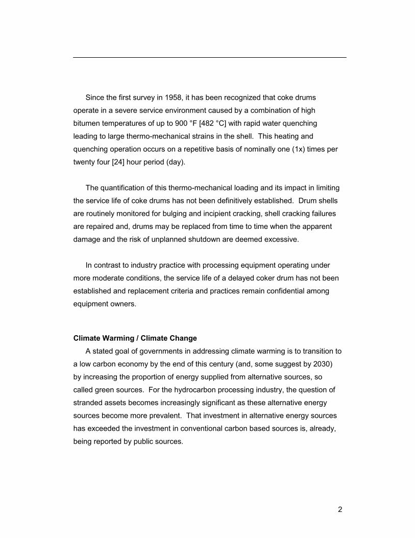
Since the first survey in 1958, it has been recognized that coke drums

operate in a severe service environment caused by a combination of high

bitumen temperatures of up to 900 °F [482 °C] with rapid water quenching

leading to large thermo-mechanical strains in the shell. This heating and

quenching operation occurs on a repetitive basis of nominally one (1x) times per

twenty four [24] hour period (day).

The quantification of this thermo-mechanical loading and its impact in limiting

the service life of coke drums has not been definitively established. Drum shells

are routinely monitored for bulging and incipient cracking, shell cracking failures

are repaired and, drums may be replaced from time to time when the apparent

damage and the risk of unplanned shutdown are deemed excessive.

In contrast to industry practice with processing equipment operating under

more moderate conditions, the service life of a delayed coker drum has not been

established and replacement criteria and practices remain confidential among

equipment owners.

Climate Warming / Climate Change

A stated goal of governments in addressing climate warming is to transition to

a low carbon economy by the end of this century (and, some suggest by 2030)

by increasing the proportion of energy supplied from alternative sources, so

called green sources. For the hydrocarbon processing industry, the question of

stranded assets becomes increasingly significant as these alternative energy

sources become more prevalent. That investment in alternative energy sources

has exceeded the investment in conventional carbon based sources is, already,

being reported by public sources.

3

Existing energy industry equipment will need to operate to the end of its useful

life and new equipment may need to be avoided. In particular, coker drums are

very expensive investments due to their size, materials and number required in

the delayed coker unit of an HPI facility.

Because of the severe service environment in which coke drums operate,

accurate determination of the thermo-mechanical loads and service life of a drum

have not been established.

Long term reliability of coker drums is impacted by thermo-mechanical

damage mechanisms associated with self constraint of the drum shell and skirt

during the formation of hot and cold temperature spots, patches and generally,

elevated temperature exposure. By assessing the imposed thermo-mechanical

strains, a more precise determination of drum fatigue may be made, allowing

better estimation of service life. This service life may be estimated for newly

fabricated drums and those drums with shell damage, such as bulging.

1.2 Thesis Objectives

The intent of this thesis is to estimate the service life of coke drums in the

newly installed condition and for drums exposed to in-service conditions.

The newly installed drum is referred to as the “undamaged” or new drum; a

drum exposed to service experiences shell distortions and is referred to as a

“damaged” drum.

The estimate will be made on a “best estimate basis” for the available data, at

hand. Each drum is unique with variation among material selection, design

details, operation and maintenance practices, operational exposure and

accumulated damage. However, the prescribed methodology in this work is

4

demonstrated for a posed drum, in the new and damaged conditions using a

specific thermal loading exposure profile.

A particular difficulty in developing the best estimate service life for this thesis

effort was the reticence of equipment owners in providing actual field data for

their equipment. The reasons likely include the cost of data collection,

competitive considerations, desire to limit publicity of equipment condition and

concerns for public liability. Hence, a fully accurate and definitive service life

determination was not possible for a specific candidate drum, as the necessary

details were not available for this work.

User responsibility: The methodology delivered in this work will be

sufficiently general to be applied for the specifics of a user’s situation. The user

will need to to be judicious in ensuring that any reliance on general data in lieu of

specific user data is acknowledged in the results.

Service life is defined to be the anticipated actual useable operating life of

the equipment compared to the Code designated design life [6]. As interpreted in

this work, service life means the amount of time a coke drum can be expected to

be crack free for the given operating exposures and capacities of the materials of

construction of the coke drum.

Determination of service life for a new / undamaged drum provides a

benchmark target for owner’s asset integrity management and future integrity

evaluations; owners currently monitor drum condition and will be able to

determine the impact of incremental damage on service life using additional

methods detailed in this work. The determination of service life for a

representative in-service drum with measured bulging provides indication of

damage progression and will affect the benchmark service life determined at

original installation.

5

This is a long-time industry problem in an industry with a history of developing

robust engineering design and assessment practices; this demands that fatigue

life determinations be made using these industry practices wherever available.

These long standing methodologies include rules for the construction of pressure

vessels, such as ASME VIII Division 1 and ASME VIII Division 2 [7].

More recently, methodologies have been developed for damage assessment

of pressure containing equipment such as API 579 – 1 / ASME FFS –1 [8].

These detailed damage assessment procedures have only been formally

developed in the last fifteen years but have not been applied in detail nor with

efficacy to the assessment of coke drums.

The reasons for this include

thermo-mechanical loading for coke drums has not been characterized

strain – life data for coke drum materials are not generally accessible

These industry practices, however, will be shown to be fundamental in

determining the undamaged and damaged coke drum service life. Calculating

service life using industry methods will be more readily accepted than alternative

methods not in conformance with the paradigms currently offered by industry.

The term “industry” is used to broadly describe equipment owners, code and

standards producing organizations (such as ASME, API, ASTM), safety

regulators and design and construction engineers involved in the construction

and operation of coke drums.

Many aspects of service life determination were available shortly after the

publication of the first drum survey i.e., the mid – 1960’s but use was inhibited by

the lack of modern computational tools

the inaccessibility of relevant industry data

the lack of initiative and cooperation by industry

6

Some of these difficulties currently persist; access to construction and

operating records, temperature and strain data continues to be guarded by

equipment owners.

It should be noted that some data presented in this thesis is obtained by

private communication and experiences gained by the author over a lengthy

career in the HPI [9]. Personal knowledge of equipment design specifications,

coke drum maintenance issues and operating practices are some examples of

this experience.

Out of necessity, there is reliance on qualitative data to benchmark the

quantitative results developed in this work. The 1996 and 2013 API surveys are

core to identifying damage trends so that correlations and conclusions can be

drawn for the analytical work presented in this thesis.

7

1.3 Operations Overview

Delayed coker drums are a specific type of coker drum in which a solid

carbonaceous residual by-product or coke is created during the thermal cracking

process in which reduced liquid bitumen feed at high temperature is injected into

the drum. The vapour portion disengages, being withdrawn overhead and the

residual solid by-product proportionately fills the drum plenum.

This by-product must be removed at the end of the oil injection / fill phase in

order to restore the drum’s empty fill volume prior to the next fill operation. Thus,

the coke drum operation is a batch process.

Coke drums experience mild pressure loads but operational temperatures are

relatively severe and large thermo-mechanical loads occur during the water

quench phase. The water quench is necessary to cool the remnant coke mass to

ambient temperature for evident reasons of safety and to minimize the

turnaround time to the next fill sequence. This is essential for profitable

operation of the unit.

These load exposures are repetitive and lead to apparent thermo-mechanical

fatigue. It was reported that there were fifty three [53] DCU’s in the United States

of America in 2003 [10].

1.3.1 System of Units

Coke drum technology was developed and continues to be led by HPI users

in the United States of America who continue to favor the US Customary system

of units, these will be used in priority to SI units for this work. There is also

advantage in using the Fahrenheit temperature scale which has finer resolution

with 1.8 F° equal to 1 C° providing more detail in quantifying differences in

temperature during transient conditions.

8

1.4 Coke Drum Operation

For reasons of economy, a minimum of two (2) drums are operated in a plant

unit to effect a semi-batch / continuous product stream, but many DCU plants

have up to eight (8) drums for production reasons as shown in Figure 1.1 [1].

These drums operate consequently in pairs; while one (1) drum is filling, the

second drum is being prepared for its fill cycle.

Figure 1.1 Photograph of Coke Drums in a Process Unit

A schematic of the delayed coke processing unit is given in Figure 1.2

illustrating entry of reduced bitumen feed, through the coker heater and then to

one of two coke drums for the delayed cracking (i.e., separation) into vapour and

solid components. The overhead vapour stream is delivered to the fractionator

for further separation into different hydrocarbon factions (“cuts”).

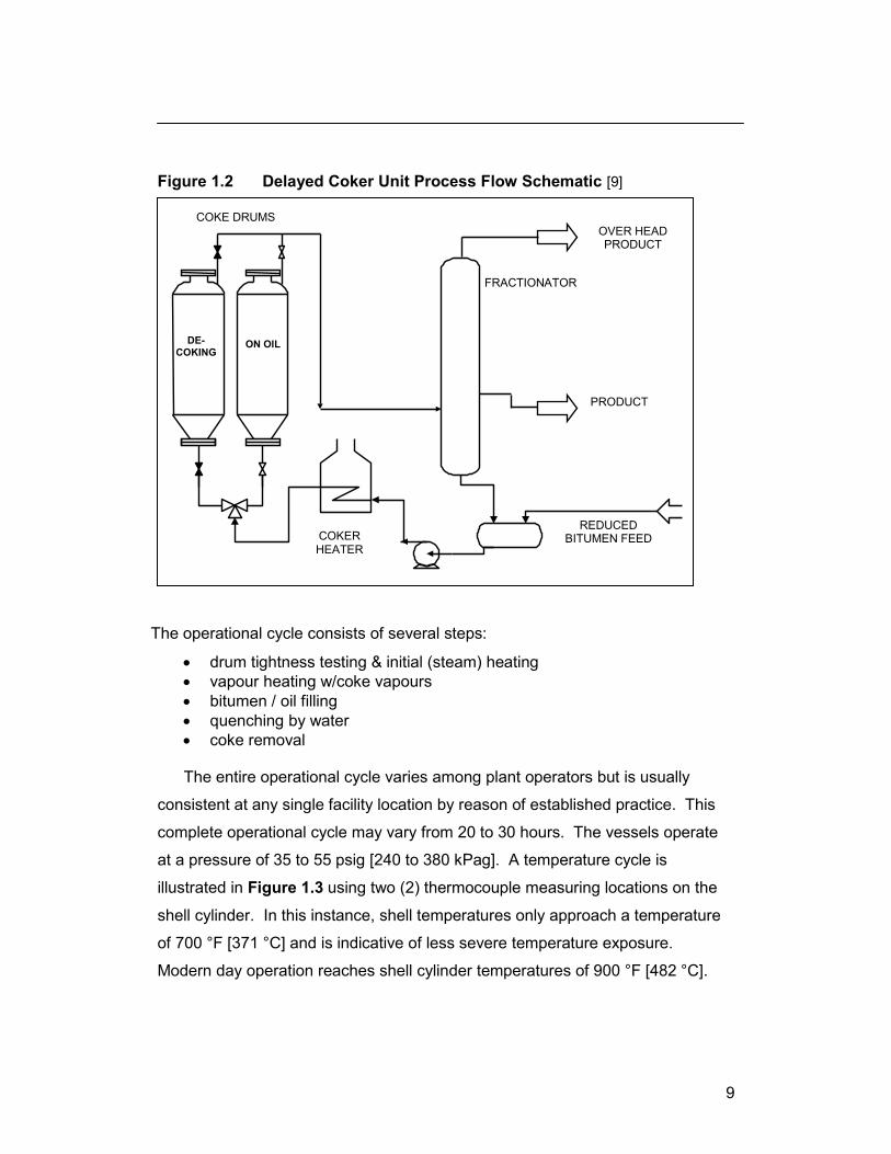
9

Figure 1.2 Delayed Coker Unit Process Flow Schematic [9]

The operational cycle consists of several steps:

drum tightness testing & initial (steam) heating

vapour heating w/coke vapours

bitumen / oil filling

quenching by water

coke removal

The entire operational cycle varies among plant operators but is usually

consistent at any single facility location by reason of established practice. This

complete operational cycle may vary from 20 to 30 hours. The vessels operate

at a pressure of 35 to 55 psig [240 to 380 kPag]. A temperature cycle is

illustrated in Figure 1.3 using two (2) thermocouple measuring locations on the

shell cylinder. In this instance, shell temperatures only approach a temperature

of 700 °F [371 °C] and is indicative of less severe temperature exposure.

Modern day operation reaches shell cylinder temperatures of 900 °F [482 °C].

COKE DRUMS

FRACTIONATOR

REDUCED BITUMEN FEED

PRODUCT

DE-

COKING

OVER HEAD PRODUCT

ON OIL

COKER HEATER

10

The number of operational cycles incurred ranges from nominally 7,500

cycles to 20,000 cycles over the course of a twenty (20) to fifty (50) year

conventional “life” of a delayed coke drum, dependent on operational specifics.

Hence, the fatigue regime is low-cycle.

Figure 1.3 Vessel Shell Temperatures during Operational Cycle in ° F [9]

Notes

1 readings from the lower elevation thermocouple 2 readings from the upper elevation thermocouple

11

1.5 Drum Size

The physical size of the drums makes this equipment visually imposing in a

refinery or oil sands plant; the drums are up to 30 feet [10 m] in diameter, 120

feet [38 m] tall and up to 220 feet [68 m] in elevation due to the need for access

below the bottom of the drum. In contrast to its large physical size, the drum

shell thickness is relatively thin, being approximately 1 inch [25.4 mm] to 1¾

inches [44.5 mm]. Early drums were only 16 feet [4,880 mm] in diameter and 35

feet [10,668 mm] in height [2]. Drums in excess of 30 feet [10 m] diameter are

being planned.

The vessel thickness is governed by a Code of pressure vessel construction.

For North American jurisdictions this is the American Society of Mechanical

Engineers or ASME Boiler and Pressure Vessel Code Section VIII Division 1

Code Rules for Pressure Vessel Construction. This Code is enforced by the

safety regulator for the specific jurisdiction where these drums are located.

1.6 Drum Construction

The ASME VIII Division 1 Code of construction addresses the design,

material selection, fabrication, inspection and examination requirements,

collectively referred to as the “construction” of the vessel.

Material selection for drums is usually low alloy clad carbon steel of various

grades to reduce the relatively large cost of these vessels; the materials listed in

Table 1.1 are both historic and, currently used for coke drums. In addition,

candidate materials, considered in current research, are also listed. A low alloy

carbon steel base material is selected for reasons of strength at the elevated

temperature of operation of the drum. The pressure retaining capability, in

operation, is provided by the base material.

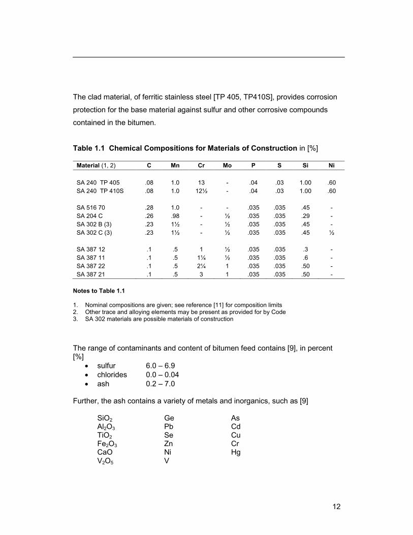
12

The clad material, of ferritic stainless steel [TP 405, TP410S], provides corrosion

protection for the base material against sulfur and other corrosive compounds

contained in the bitumen.

Table 1.1 Chemical Compositions for Materials of Construction in [%]

Material (1, 2) C Mn Cr Mo P S Si Ni

SA 240 TP 405 .08 1.0 13 - .04 .03 1.00 .60

SA 240 TP 410S .08 1.0 12½ - .04 .03 1.00 .60

SA 516 70 .28 1.0 - - .035 .035 .45 -

SA 204 C .26 .98 - ½ .035 .035 .29 -

SA 302 B (3) .23 1½ - ½ .035 .035 .45 -

SA 302 C (3) .23 1½ - ½ .035 .035 .45 ½

SA 387 12 .1 .5 1 ½ .035 .035 .3 -

SA 387 11 .1 .5 1¼ ½ .035 .035 .6 -

SA 387 22 .1 .5 2¼ 1 .035 .035 .50 -

SA 387 21 .1 .5 3 1 .035 .035 .50 -

Notes to Table 1.1

1. Nominal compositions are given; see reference [11] for composition limits 2. Other trace and alloying elements may be present as provided for by Code 3. SA 302 materials are possible materials of construction

The range of contaminants and content of bitumen feed contains [9], in percent [%]

sulfur 6.0 – 6.9

chlorides 0.0 – 0.04

ash 0.2 – 7.0 Further, the ash contains a variety of metals and inorganics, such as [9]

SiO2 Ge As Al2O3 Pb Cd TiO2 Se Cu Fe2O3 Zn Cr CaO Ni Hg V2O5 V

13

Materials of construction are also referenced by their nominal composition as

C – Mo or Cr – Mo steels for the base layer or by industry designator as TP 405

and TP 410S stainless steel for the clad layer.

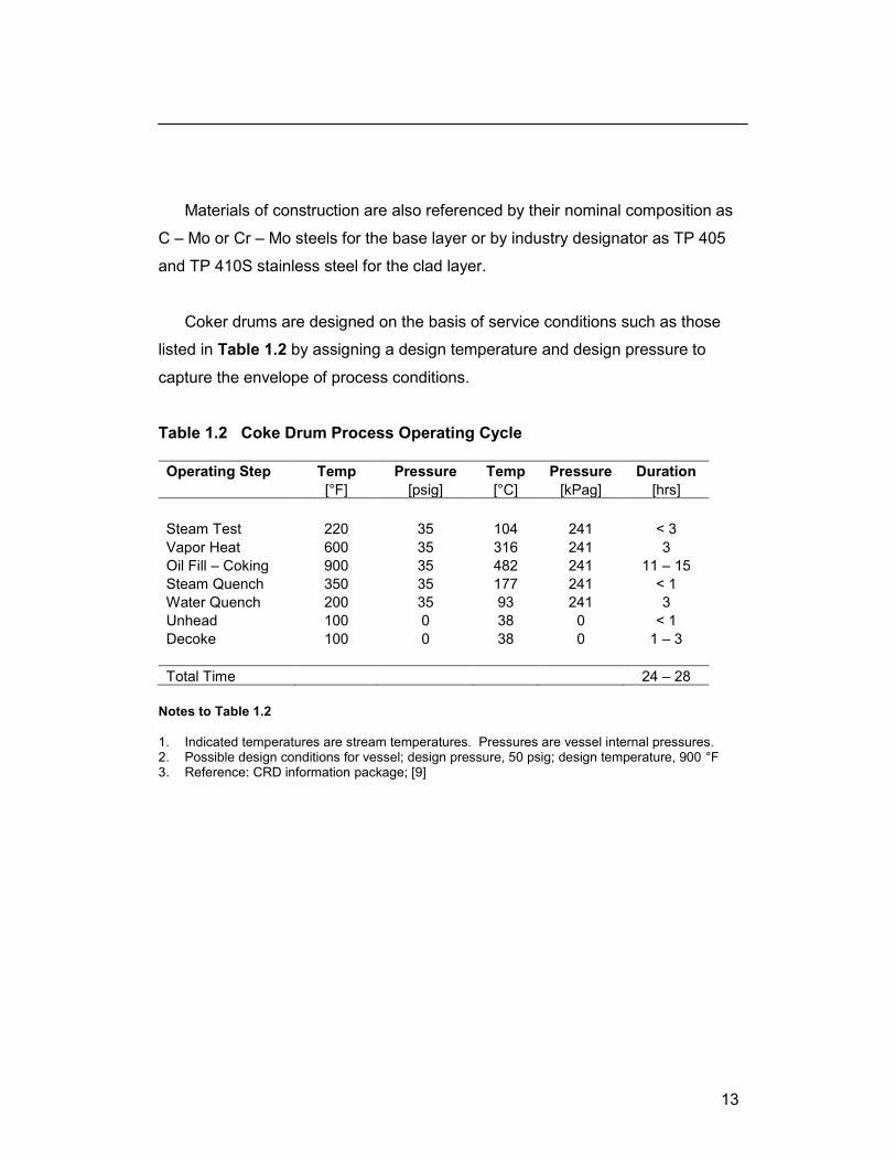
Coker drums are designed on the basis of service conditions such as those

listed in Table 1.2 by assigning a design temperature and design pressure to

capture the envelope of process conditions.

Table 1.2 Coke Drum Process Operating Cycle

Operating Step Temp Pressure Temp Pressure Duration

[°F] [psig] [°C] [kPag] [hrs]

Steam Test 220 35 104 241 < 3

Vapor Heat 600 35 316 241 3

Oil Fill – Coking 900 35 482 241 11 – 15

Steam Quench 350 35 177 241 < 1

Water Quench 200 35 93 241 3

Unhead 100 0 38 0 < 1

Decoke 100 0 38 0 1 – 3

Total Time 24 – 28

Notes to Table 1.2

1. Indicated temperatures are stream temperatures. Pressures are vessel internal pressures. 2. Possible design conditions for vessel; design pressure, 50 psig; design temperature, 900 °F 3. Reference: CRD information package; [9]

14

1.7 ASME VIII Construction Codes

The two Code divisions of interest, Division 1 and Division 2 provide two

different levels of construction effort. The former uses a simplified design

philosophy, requiring reduced engineering skill in its implementation while the

Division 2 mandates a robust principles based engineering approach with

certification and filing of a manufacturer’s design report to be completed by a

registered professional engineer.

The primary pressure design consideration of the Division 1 Code of

construction is to provide a design resistant to collapse (i.e., general yielding)

failure under pressure loading while in service.

The Code lists other pertinent loads to be considered by the designer

including cyclic and dynamic reactions due to pressure or thermal variations,

temperature gradients and differential thermal expansion. Specific

methodologies are not presented in the Code. Unfortunately, definitive data is

not provided to designers and these particular loads are ignored in practice,

precluding a comprehensive design treatment of the vessel.

Safety regulators have not shown the same interest in these secondary

loads. The regulators are focused on those loads causing “collapse” of a vessel,

i.e., those sustained loads which would cause through-wall membrane yielding of

the vessel. This collapse failure is modeled on use of an elastic – perfectly

plastic material behavior model.

These sustained loads are specifically

pressure

live weight

dead weight

15

The Code does not require calculation of stress but rather, only a design

pressure thickness which must be able to contain the equivalent hydrostatic

pressure from the combined internal pressure and weight loads. The Code is

motivated by a “design by rules” approach to reduce engineering involvement;

hence, vessel stresses are not explicitly calculated in design; rather, the designer

calculates a pressure thickness using the temperature dependent allowable

stress, the quantity “S” in Table 1.3, assigned for the material.

In contrast to the Division 1 Code, the alternative rules of the ASME VIII

Division 2 Code practice methodology categorizes stresses as primary,

secondary and peak and limits these based on consideration of their failure mode

and loading source. Engineering skill and judgment are required to implement

the process as the load – stress impact are not always evident. These limits are

designated as “design by analysis” and their motivation is broadly divulged in the

Code. Specific details, insights and background, however, are not discussed and

the certifying engineer must take initiative to understand the underlying principles

contained in these provisions. Some of these provisions can be readily

recognized from strength – of – materials considerations; others, may be

experientially based while others may be obscure. Ancilliary documents and

practice studies are available, while original work may also need to be

undertaken and is encouraged by the Code for specific designs.

The Division 2 Code design considerations are

to limit loads to general and local primary stress limits

to limit loads to secondary stress limits

to limit loads to peak stress limits

16

For example, general membrane stresses, designated Pm stresses need to

be limited to the allowable design stress, Sm which is derived as a function of the

material specified minimum yield strength, SMYS or as a function of specified

minimum tensile strength, SMTS. The internal pressure load develops Pm type

stresses.

Cyclic thermo-mechanical loads give rise to fatigue failure which is limited to

a peak stress limit. The two types of failures arising from exceeding the limit on

general membrane stress and exceeding the limit on peak stress are very

different. Consequently, regulators simply treat the failures caused by cyclic

loads as reliability failures which have experientially not warranted the same

consideration as failure associated with insufficient design pressure thickness.

Cyclic loads are assumed to cause leak-type failures in coke drum vessels when

they are not adequately designed to avoid fatigue failure. This stance not

appropriate, in general, for industry applications since they may contain

dangerous and lethal service fluids.

Industry practitioners have limited coke drum construction to the ASME VIII

Division 1 Code on account of these considerations. Using the relevant Code

such as ASME VIII Division 1, for a cylindrical shell section, the pressure

thickness of interest, from the Code formula is derived from strength of materials

considerations as: [6]

PES

RPt

6.0

where, using consistent units: t ≡ the required pressure thickness, P ≡ the design pressure of the component, R ≡ the radius of the cylindrical section, S ≡ the allowable stress as set out in the Code for the design temperature, E ≡ weld joint efficiency for the component, dimensionless

[1.1]

17

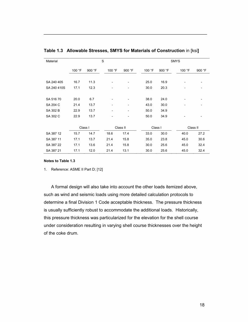
Temperature dependent allowable stress values are provided in Table 1.3 for

the various materials of interest.

Therefore, a coke drum will be designed for pressure thickness, “ t ” using the

internal design pressure and static head from dead and live weight loads at the

appropriate temperature water,

P = pressure + static head = 55 psig + (120 ‘ elevation head / 2.3 ‘ / psi), head = 107.2 psig

R = 30’/2 * 12 = 180 inches S = 15,800 psi at 900 °F based on using either of SA 387 11 or 22 Class 2 E = 1.0 since welds are fully radiographed hence,

]31[226.12.1076.01800,15

1802.107

6.0mminches

PES

RPt

or (1.1)

1¼” [32mm] for the base (i.e., pressure containing) layer,

This demonstrates the practice of constructing the coke drum with relatively

thin shell wall thicknesses. Note that the density of bitumen feed to the coke

drum [52 lbf / ft3] is slightly less than the density of water [60.0 lbf / ft

3] at

operating conditions. Coke density is usually stated as 58 lbf / ft3. Water fill is

specified to the top of the vessel while a coke / water mix is specified to a normal

fill height of approximately 80% of vessel height. By Code, shell thickness is

calculated at drum design temperature.

18

Table 1.3 Allowable Stresses, SMYS for Materials of Construction in [ksi]

Material S SMYS

100 °F 900 °F 100 °F 900 °F 100 °F 900 °F 100 °F 900 °F

SA 240 405 16.7 11.3 - - 25.0 16.9 - -

SA 240 410S 17.1 12.3 - - 30.0 20.3 - -

SA 516 70 20.0 6.7 - - 38.0 24.0 - -

SA 204 C 21.4 13.7 - - 43.0 30.0 - -

SA 302 B 22.9 13.7 - - 50.0 34.9

SA 302 C 22.9 13.7 - - 50.0 34.9 - -

Class I Class II Class I Class II

SA 387 12 15.7 14.7 18.6 17.4 33.0 30.0 40.0 27.2

SA 387 11 17.1 13.7 21.4 15.8 35.0 23.8 45.0 30.6

SA 387 22 17.1 13.6 21.4 15.8 30.0 25.6 45.0 32.4

SA 387 21 17.1 12.0 21.4 13.1 30.0 25.6 45.0 32.4

Notes to Table 1.3

1. Reference: ASME II Part D; [12]

A formal design will also take into account the other loads itemized above,

such as wind and seismic loads using more detailed calculation protocols to

determine a final Division 1 Code acceptable thickness. The pressure thickness

is usually sufficiently robust to accommodate the additional loads. Historically,

this pressure thickness was particularized for the elevation for the shell course

under consideration resulting in varying shell course thicknesses over the height

of the coke drum.

19

Figure 1.4 Typical Coke Drum Shell Plate Layout

Shell courses are typically ten (10) feet [3.05 m]

wide allowing the course design thickness to be

conveniently varied over the height of the drum. Six (6)

to ten (10) or more shell courses are assembled to

form the overall height of the cylinder portion of a

modern drum. Figure 1.4 shows the typical shell

layout with staggered vertical shell seams (a Code

practice). The thickness of cladding (for corrosion

protection) is arbitrarily chosen as 0.120 inches [3 mm]

from industry experience but can vary for individual

equipment per Owner preference.

To address thermo-mechanical loading, which has

been recognized since the first survey in 1958,

equipment owners have provided a general statement

that a thermal load shall be considered in the design.

However, no detailed definition of this load is provided

in construction specifications and hence, design submissions do not contain any

consideration of these loads other than listing the design temperature.

Nonetheless, the industry has, by virtue of broader experience, incorporated

fatigue compatible design features in recent modern coker drum construction.

Fatigue compatible fabrication, listed in Code practices, is implemented in

modern coker drum construction, including

use of flush weld profiles for all shell weld seams

uniform shell plate thickness throughout the height of the drum

fatigue compatible shell to skirt weldments such as integral transition

top and bottom head located feed nozzles only, with no nozzles located on the main shell cylinder

elimination of insulation support rings welded to the shell cylinder

elimination of the derrick attachment to the top head of coker drum; modern practice is to support the derrick on an external structural frame

20

Figure 1.5 shows an independently supported derrick structure atop the drums

Figure 1.5 – Coke Drum Unit Derrick Structures

21

1.8 Thesis Summary

Delayed cracking unit coke drums are a vital technology for the HPI in the

processing of heavy molecule hydrocarbons into marketable products. However,

their use since the early 1930’s has been problematic in realizing longer term

integrity and reliability; industry engineering practitioners have been unable to

definitively identify the damage mechanisms causing shell bulging and cracking

and the impact on vessel service life.

Although a number of industry surveys, papers and practice documents have

been published, there has been no satisfactory application of the body of

knowledge to resolving coke drum service life deficiencies. Practitioners have

listed the complexities of assessing service loads and damage mechanisms as

the primary difficulty in determining service life and, thus, motivating the use of

simplified, contrived and unsatisfactory damage criteria.

Our thesis demonstrates that the basic industry methodology has been

available since the mid – 1960’s but has been inadequately interpreted and

incorrectly applied to the problem of coke drum service life determination. In

addition, the basic methodology must be augmented in specific areas where the

methodology is insufficiently detailed and inadequate for application to service-

exposed equipment. These deficiencies in application have lead to the current

inability to determine service life for either a new or a damaged coke drum.

Premature retirement of equipment from service has led to economic loss for

equipment owners and the inability to assess quantitatively the safety risks from

damaged equipment to which industry workers may be exposed.

22

CHAPTER 2 LITERATURE REVIEW

The HPI industry has provided a number of surveys since 1958 and more

recently, technical reports specifying assessment methodologies to evaluate

general pressure vessel damage and demonstrate suitability for continued

operation. A limited number of papers have also been produced.

Industry surveys provide operational and maintenance information but have

not elicited from equipment owners more quantified data which would assist

more rigorous engineering analysis. However, these surveys do provide

sufficiently reasonable data to qualitatively support the analytical efforts of the

thesis work.

2.1 Industry Surveys

Weil & Rapasky, 1958 This survey of 16 coke drums was undertaken by an

industry engineering contractor, MW Kellogg Company, Houston, Texas to

address the number of reports of equipment distress. The paper indicates that

coke drum temperatures operated to a temperature of 800 °F [427 °C] over a 24

to 48 hour cycle [3].

Drum dimensions were listed to be from 12 to 19 feet [3.6 m to 5.8 m] in

diameter, 37.5 to 69.2 feet [11.4 m to 17.6 m] in straight side cylinder length,

fabricated from carbon [SA 285 C] and low alloy carbon steel [SA 204 C i.e., C –

½ Mo] steel with TP 405 or TP 410 stainless cladding.

Severe shell diameter growth, bulging and skirt cracking were the major

issues affecting drum integrity. The survey established that temperature

gradients during quenching were severe with gradients of up to 27.1 F° per inch

[15 C° / 25.4 mm] measured on the external drum shell surface. Channeling of

quench water was identified to account for the gradients being noted in the lower

shell courses but not in the bottom cone of the vessel.

23

The survey proposed an operating criteria to control the temperature

gradients, the Unit Quench Factor [UQF] by throttling water flow to the coke drum

to a threshold value. Slower water addition correlated with less bulging and

cracking damage. This suggested water quench periods of 6 to 8 hours.

This survey established the notion that shell bulging resembled a ballooning

of individual shell courses that migrated from the bottom course upwards.

Figure 2.1 illustrates this concept. Skirt cracking was identified as the most

widespread maintenance difficulty occurring within 550 to 2,330 operational

cycles, i.e., within 1½ to 7 years after startup.

Figure 2.1 Progressive Bulging Damage of Coke Drums

Normal shape

Stage 1 Onset of bulging

Stage 2 Girth seams gain definition

Stage 3 Developed

bulged shape

24

Thomas, 1968 & 1980 Two industry surveys were reviewed by Thomas. A

summary of the 1968 API report revealed [4]

the survey was motivated by drum shell cracking

cracking in the shell followed minor to severe shell bulging

cracking is circumferential at weld seams

cracking may be in the apex or valley of shell bulge

thin wall vessels experience cracking sooner

C – ½ Mo drums appear to be more crack sensitive than carbon steel drums

The 1980 survey by Thomas reported on 62 drums

a shift from carbon steels and C – ½ Mo to Cr – Mo steels had taken place from 1960 through the 1970’s

operating temperatures had increased to 900 °F [482 °C]

drum diameter had increased to 22 feet [6.7 m]

earliest cracking varied from 7 years (carbon steel) and 8 years (C – ½ Mo) to 12 years (Cr – Mo)

drums with no cracking varied in service to 32 years (carbon steel), 22 years (C – ½ Mo) and 11 years (Cr – Mo)

no correlation was found between drum thickness and first cracking for C – ½ Mo and Cr – Mo steels

API 1996 Survey The survey updated the prior surveys with the following

information [13]

the survey reported on 145 drums

new drum material selection showed a trend to increase Cr – Mo content

clad material is either TP 410 or TP410S

no correlation was found between drum cracking and fill cycle time

drum operating parameters such as initial quench rate and proofing quench practice rather than metallurgy changes, appear to have a greater influence on drum cracking

skirt cracking was reported by 73% of the surveyed companies; of the 23% that replaced skirts, re-cracking eventually occurred 43% of the time

the first bulge appeared sooner than first through-wall cracks.

shell bulging was reported by 57%. Shell cracking was reported by 57%

of the drums that bulged, 87% also experienced cracks; cracking without bulging was reported only by 6%

when cracking was reported, it occurred in the circumferential direction 97% of the time. Most of the cracks were located in courses 3, 4, and 5 (course 1 is at the bottom)

25

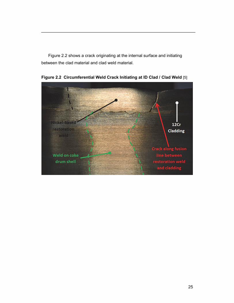
Figure 2.2 shows a crack originating at the internal surface and initiating

between the clad material and clad weld material.

Figure 2.2 Circumferential Weld Crack Initiating at ID Clad / Clad Weld [5]

26

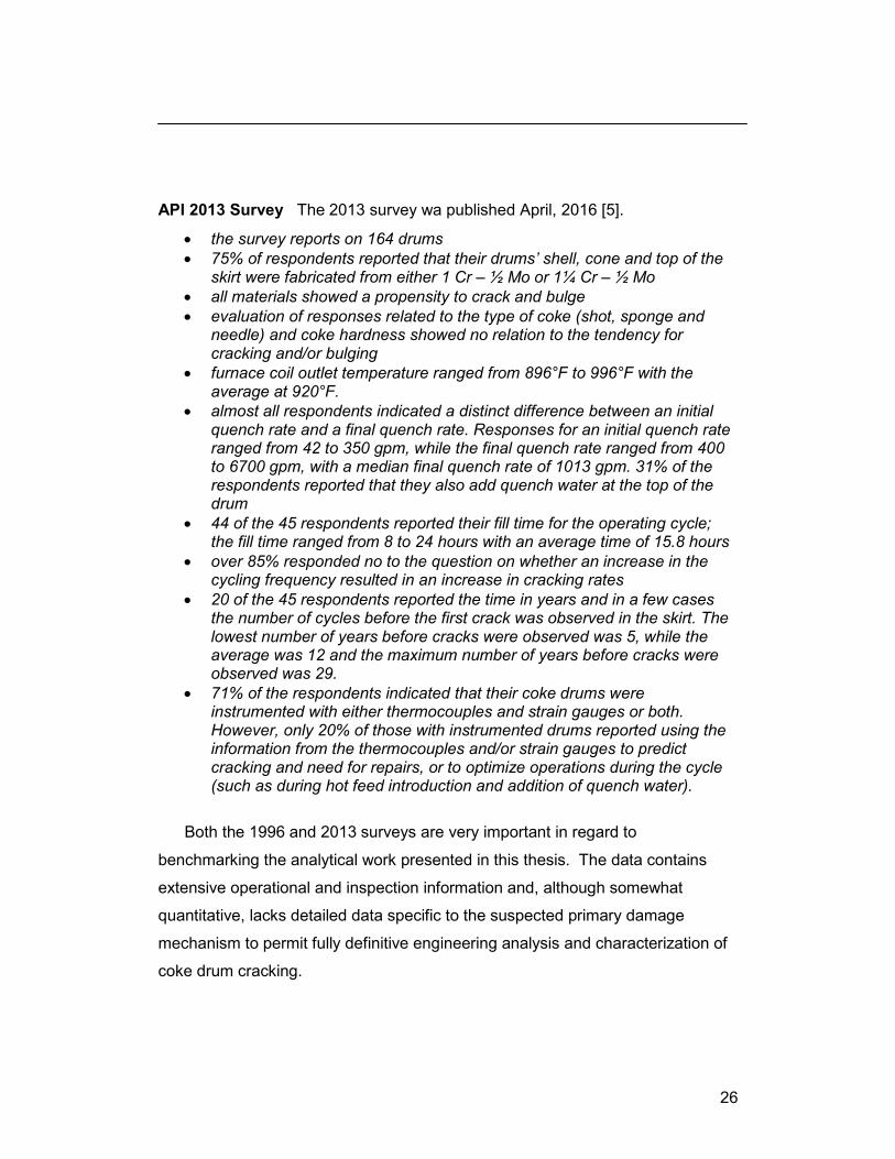
API 2013 Survey The 2013 survey wa published April, 2016 [5].

the survey reports on 164 drums

75% of respondents reported that their drums’ shell, cone and top of the skirt were fabricated from either 1 Cr – ½ Mo or 1¼ Cr – ½ Mo

all materials showed a propensity to crack and bulge

evaluation of responses related to the type of coke (shot, sponge and needle) and coke hardness showed no relation to the tendency for cracking and/or bulging

furnace coil outlet temperature ranged from 896°F to 996°F with the average at 920°F.

almost all respondents indicated a distinct difference between an initial quench rate and a final quench rate. Responses for an initial quench rate ranged from 42 to 350 gpm, while the final quench rate ranged from 400 to 6700 gpm, with a median final quench rate of 1013 gpm. 31% of the respondents reported that they also add quench water at the top of the drum

44 of the 45 respondents reported their fill time for the operating cycle; the fill time ranged from 8 to 24 hours with an average time of 15.8 hours

over 85% responded no to the question on whether an increase in the cycling frequency resulted in an increase in cracking rates

20 of the 45 respondents reported the time in years and in a few cases the number of cycles before the first crack was observed in the skirt. The lowest number of years before cracks were observed was 5, while the average was 12 and the maximum number of years before cracks were observed was 29.

71% of the respondents indicated that their coke drums were instrumented with either thermocouples and strain gauges or both. However, only 20% of those with instrumented drums reported using the information from the thermocouples and/or strain gauges to predict cracking and need for repairs, or to optimize operations during the cycle (such as during hot feed introduction and addition of quench water).

Both the 1996 and 2013 surveys are very important in regard to

benchmarking the analytical work presented in this thesis. The data contains

extensive operational and inspection information and, although somewhat

quantitative, lacks detailed data specific to the suspected primary damage

mechanism to permit fully definitive engineering analysis and characterization of

coke drum cracking.

27

2.2 Industry Practices

Industry may collaborate either through industry trade groups such as the

ASME, API, DNV, EWI and others. In addition, joint industry programs [JIP] may

be undertaken either publicly or exclusively among the JIP sponsors.

2.2.1 Industry Codes, Standards and Technical Reports

Industry has developed Codes and Standards since the first ASME Code

committee was established in 1911 for the purpose of formulating standard rules

for the construction of steam boilers and other pressure vessels [6].

The API and the ASME collaborated to produce a joint Code for Unfired

Pressure Vessels first published in 1934. This effort has evolved into the ASME

VIII Division 1 and ASME VIII Division 2 Codes for unfired pressure vessel

construction. Reference to the term Code may mean either of these two Code

sections, in this work. Collectively, the ASME Boiler and Pressure Vessel Code

refers to twelve (12) sections covering heavy industry, nuclear facilities and

commercial equipment.

Since pressure vessels are usually regulated by a jurisdiction through a

competent regulator, other codes may be used in these jurisdictions.

ASME VIII Division 1

The basic construction Code for coke drums is ASME Section VIII Division 1

Rules for Construction of Pressure Vessels [6]. Engineering specifications

provided by engineering contractors and equipment owners specify this Code

and provides the “design by rules” determination of pressure thickness. Other

Codes and standards are used to assess the coke drum when it has sustained

damage such as bulging and cracking.

28

ASME VIII Division 2

ASME Section VIII Division 2 is a construction document which uses a

“design by analysis” approach in the design of pressure vessels as an alternative

to the “rules based” design of ASME VIII Division 1. As indicated, Division 2

provides an engineered approach to vessel design using detailed stress

calculation, stress categorization and stress criteria to substantiate the design [7].

A methodology to address fatigue is provided which is motivated by fatigue

initiation and uses the classic Wöhler S – N, stress – cycle life, design approach.

However, pseudo – elastic stresses are used when yield strength is exceeded for

simplification. More sophisticated analysis bases such as elastic – plastic

methods are also allowed.

Fatigue curves are provided for smooth bar and welded joint specimens.

Base material properties are designated as smooth bar design curves. The

smooth bar fatigue curves may be used on components with or without welds.

A weld surface fatigue strength reduction factor [FSRF] is used to account for

the effect of a local structural discontinuity or weld joint on the fatigue strength. It

is the ratio of the fatigue strength of a component without a discontinuity or weld

joint to the fatigure strength of a component with a discontinuity or weld joint.

The concept is symbolized by Kf , in the Code, and values of the FSRF range

from 1.0 to 4.0. The Code states that fatigue cracks at pressure vessel welds are

typically located at the toe of a weld. For as-welded and weld joints subject to

post weld heat treatment, the expected orientation of a fatigue crack is along the

weld toe in the through-thickness direction, and the structural stress normal to

the expected crack is the stress measure used to correlate fatigue life data.

Design fatigue curves for welded joints are presented on the basis of welded

joint design with statistical confidence intervals varying from ± 68% to ± 99%, i.e.

± 1 to ± 2.33 .

29

This Code also provides for experimental stress and fatigue analysis. When

invoked, temperature applicability is limited to not more than 700 °F [371 °C] and

cyclic exposure to not exceed 50,000 cycles. The determination of fatigue

strength uses a number of strength reduction factors to account for

size

surface finish

cyclic rate

test temperature

thermal skin stress

statistical variation

The strength reduction factors are prescribed by closed form expression.

The establishment of a design curve is complex due to the number of factors and

required manipulations.

The Code states a preference that the fatigue strength reduction factor be

preferably determined by performing tests on notched and unnotched specimens,

and calculated as the ratio of the notched stress to the unnotched stress for

failure [7].

API 579 – 1 / ASME FFS-1 Fitness for Service

This is a dual marked industry practice document sponsored by API and

ASME to determine the fitness of in-service equipment for continued operation in

the event that damage is encountered in the equipment [8].

Stress analysis is required for many of the damage assessments and is

detailed in Annex B1 of the standard. The methodology parallels ASME VIII

Division 2 but does have peculiarities.

30

MPC Coke Drum Evaluation Report, 1999

An industry collaboration in 1999 resulted in confidential publication of the

Materials Property Council [MPC] coke drum report. Sponsorship as a group

project was provided by several DCU technology licensors, equipment owners

and fabricators. The MPC is a not-for-profit scientific and technical corporation

loosely aligned with the ASME. The report has restricted access [14].

The primary purpose of this effort was to establish evaluation procedures for

coke drums in consideration of materials selection, evaluation software for

bulging and cracking damage, repair guidelines, materials properties data and

provision of a laser scan database for use with a software package called

CokerCola™. Parametric finite element studies were completed to support the

software.

The report provided focus on the operating conditions of coke drums and the

role of water quenching in the development of thermo-mechanical strains. This

provided definition to the vague descriptions of thermal fatigue stated in prior

work.

Using experimental data from monitoring an operating coke drum,

temperature and strain data were collected. The intent was to provide default

histograms for use with the software; but, actual histograms can also be used to

particularize results to the users’ coke drums.

31

Fatigue failure is calculated in a two step process, crack initiation and crack

propagation. Crack initiation is determined by the Manson – Coffin – Basquin

expression (also known as “universal slopes”) [15].

cff

bf

fNN

E

22

2

(2.1)

The exponent values b, c are calculated from the experimentally derived data

for the other parameters contained in the expression.

Material properties are provided in an internal database and presented for

interest. The material properties for welds are not differentiated. The source of

the fatigue properties is not stated and inconsistent with properties listed in [12].

Also of interest is the uniformity in the listed values; the properties for TP 405 and

TP410S stainless steels being identical to C – ½ Mo and Cr – Mo.

Crack propagation is modeled by use of the Paris equation available in the

fracture mechanics literature [15].

For convenience, the Paris equation is provided herein;

da / dN = C ∙ Km (2.2)

Strain histograms are included in the MPC document as an internal database

and are categorized as light to severe. The strains are presented as strain

ranges with an average strain range of

794 - 435 for -1 log standard deviation

+ 966 for +1 log standard deviation

The user may input temperatures, temperature gradients or strain gauge

readings to generate a strain histogram for use by the program.

32

Figure 2.3 is a plot of the strain distribution with a negative skew in the data leading to modeling of the data as lognormal.

Figure 2.3 Strain Distribution as Provided by MPC [14]

The strain range is asymmetric since the strains are lognormally distributed.

The strains were also confirmed to be strain ranges and determined based on

observation of strains during the quench wave ascribed to the rising water level

during the quench phase.

Temperature gradients of approximately 1 F°/ inch to 14 F°/ inch are used in

the software module. The actual temperature distributions were not used in the

accompanying numerical analysis supporting the software.

A significant result of the MPC work is the assertion that strains could be

adequately calculated through linear – elastic analysis.

33

Although bulges were evaluated, all bulge profiles use smooth transitions.

The bulges were said to have little or no effect on thermal stresses due to axial

temperature gradient but influence thermal stresses due to a circumferential

gradient.

In general, feedback on the efficacy of the software is not widely available.

Informal comment from a CRD partner indicates the software and methodologies

are not sufficiently predictive or accurate to use results as a decision

management tool.

API TR 934 – G

The API TR 934 – G is a comprehensive document covering

a survey undertaken in 2013

construction

maintenance

operations

fitness for service evaluation The release document contains some significant findings for consideration for

this thesis;

thermal fatigue is to be evaluated to the fatigue curves of ASME VIII Division 2; use limitations in temperature to 700 °F [371 °C] are not considered prohibitive

alternatively, a fracture mechanics approach for identified cracks may be used; the use of industry practice documents API 579 / ASME FFS-1 may be utilized

Cr – Mo materials are used in the Class 2 condition

Cr – Mo materials in higher minimum yield strength to 60 ksi [415 MPa] are available for improved resistance to shell cylinder bulging

reference to “ratcheting” mechanism leading to drum distortion

bulging is attributed to differences in shell metal temperature

circumferential cracking with and without noticeable bulging

an alternative basis for material selection is fracture ductility such as exhibited by C – ½ Mo rather than Cr – Mo steels; bulging may be more prevalent but the tendency to crack will be reduced due to better ductility

34

The supply of the usual Cr – Mo materials of construction in minimum yield

strengths to 60 ksi [415 MPa] would be considered special order since typical

minimum yield strengths are much less than 60 ksi [415 MPa].

The document makes use of the terms “hot spot” and “cold spot” in regard to

the design of the coke drum feed system; a single nozzle entry at the bottom of

the vessel is seen to provide biased flow and promotes “hot / cold spots” on the

vessel shell cylinder. A dual inlet nozzle is opined to better simulate a bottom

center fluid up-flow to minimize “hot / cold spot” formation during the feed and

quench phases [5].

BS PD 5500

British Standard PD 5500 Specification for Unfired Fusion Welded Pressure

Vessels provides requirements for the assessment of pressure vessels subject to

fatigue [16].

Although all North American jurisdictions use the ASME Code for pressure

vessel construction and the dual marked standard, API 579 –1 / ASME FFS – 1

for fitness for service assessments, using PD 5500 for guidance in fatigue

assessment is warranted based on its more transparent experimental data set

including an explicit experimentally oriented treatment of welded construction and

weld defects. The methodology is also much more streamlined to use thus

making it more practical for industrial users compared to the “clean rewrite”

edition of ASME VIII Division 2.

35

Major differences to the ASME Code approach are

the nominal stress range is used in region of fatigue cracking to enter S – N curves

the stress range is used to enter S – N curves, regardless of applied mean stress

fatigue assessment is based on the primary plus secondary stress; i.e., direct stress is used [C.3.3.1]

thermal stresses are treated as secondary stresses

explicit attention is given to weld quality, both surface and through thickness condition; the limit on internal defects is more stringent

justification for use of the design curve for unclassified details is based on testing; Table C.5 provides a factor to check against the published curves – this appears to be a design margin

Consistent with the ASME Code approach are;

low cycle data uses a pseudo-elastic stress range ( i.e., strain range multiplied by elastic modulus)

S – N curves applicable to temperatures up to 350 °C [662 °F], creep is to be accounted for if the curves are used at higher temperatures

Palmgren – Miner rule is used for limiting damage accumulation

36

2.2.2 Industry Trade Papers

Industry journals, conferences and symposia provide additional perspectives

and insight into coke drum issues. Most are provided by the ASME Journal of

Pressure Vessels and Piping and ASME PVP conference papers.

Local venues, especially in the US Gulf coast region provide opportunities for

data sharing and networking, such as Stress Engineering Services Inc., a

specialty engineering and design firm which hosts a coke drum reliability

workshop on a regular basis in Houston, Texas [17].

Ramos, Rios Two papers by Ramos and Rios et al. explored low cycle fatigue

tests for 1 Cr – ½ Mo and 1¼ Cr – ½ Mo low alloy carbon steel in base metal and

welds in support of examining the fatigue life for the conventional shell to skirt

connection and shell cylinder [18], [19].

Figure 2.4 presents a portion of the – N fatigue life testing observed by original

testing in support of their work. Observations from the data indicate

differing base metals exhibit similar – N life curves

weld joints exhibit similar – N life curves, but lower than the base metal

37

Figure 2.4 Strain – Cycle Life for Cr – Mo Base and Weld Metal

Notes

1 Open symbols present results from weld material 2 Closed symbols present results for wrought materials

The second paper describes a field study using temperature and strain gauge

monitoring. A thermograph was presented which displayed a cold spot in the

shell more than 400 F° cooler than the surrounding shell area and had formed

within a 15 minute period. They noted that “large strains will result from this

temperature distribution due to differential thermal contraction”. The paper did

not explore the extent to which these cold spots contributed to the observed

strain ranges. Coke drum damage was ascribed to “low cycle fatigue [LCF] is the

main cause of damage in most coke drums. LCF is caused by cyclic strains.” A

cyclic strain range was defined as

= max (i) – min (i) at a point (2.3)

where, max (i) and min (i) were defined to be the maximum and the minimum

observed strain measured by strain gauge in one complete cycle. The cycle

defined is an operational cycle.

38

The paper showed that lower shell strain ranges were related to reduced

quench water rates.

Penso, Lattarulo et al. This paper from 1999 provides a thorough review of

metallurgical analysis from coke drums and listed four different types and sites

for cracking initiation and propagation [20]

deep cracks in the clad HAZ

shallow cracks in the clad

interbead cracks in the high nickel weld

inclusion cracks in the base metal HAZ

The parameters promoting crack initiation and propagation were listed as

grain growth in the HAZ

weld toe geometry

strength mismatch among welds, clad metal and base metal

thermal shock

Boswell, Farraro A 1997 paper on the experiences of a coke drum located at a

refinery in Lake Charles, Louisiana suggests that the coke drum problems are

accounted for by [21]

repairs to the shell circumferential seams near large distortions,

skirt junction cracking, and

nozzle failure.

Presumably, failures of shell circumferential seams prompt repairs and these

are more likely needed at large distortions. The paper also makes mention of

local hot spots being identified and shows stress results for a quench cycle which

attains a calculated strain of 3,090 . This value matches the data of Ramos

and Rios which showed a maximum strain of 3,400 .

39

Boswell and Farraro introduce additional notions

that the material elastic yield strength is related to low cycle fatigue and particularly the 2 · SY limit

bulging is determined by the relative strength of the circumferential weld seam and the base metal

a mechanical stress ratchet develops between weld seam and base metal

when the weld seam has a higher yield strength than the base metal, the base metal distorts relative to the weld seam; the opposite occurs when base metal has higher yield strength than the weld metal

wall thinning is suggestive of low cycle fatigue

material properties are to be determined from samples removed from the drum

the studied coke drum was built in 1968 and scheduled for replacement in 1996, a run of 28 years; accumulated cycles were approximately 5,497 cycles

a fatigue life of 4,390 cycles was predicted using ASME VIII Division 2 Figure 5-110.1 which matches experience

there are three stages to fatigue failure; from 50% to 95% of cyclic life cracks will grow to one-half (½) their final catastrophic size

operating beyond 95% of cyclic life is dependent on finding, measuring and repairing the crack

Church, Lim, Brear et al. Church describes a damage mechanism for coke

drums occurring during the quench phase involving “contraction of a ring of the

shell with a step change in diameter to the ‘hot’ coke drum above this quenched

ring. This cold to hot shell transition (vase) rises up the drum wall with the steam

and leads to the generation of thermal stresses ” [22].

Church considers a stress-based approach attributing stress development to

through wall temperature gradients and the vasing effect from rising quench

water. The stress amplitudes are derived, though, from measured strain

amplitudes which are extracted from a distribution of measured strains.

At that point, Church describes a probabilistic methodology to predict the

number of cycles to crack initiation, using the S – N fatigue life methodology and

through-wall failure is determined by a linear – elastic fracture mechanics

approach using the Paris expression (equation 2.2).

40

The strain or stress distribution is not provided but a cumulative probability

distribution is shown that is benchmarked against an actual coke drum. The

graph shows the following

crack initiation begins at 1,000 cycles with 0.0001% probability, exponentially rising to 100% at 40,000 cycles

cracking was actually observed at 2,000 and 3,000 cycles

through – wall failure was predicted with 0.0001% probability at 4,000 cycles, rising exponentially to 100% at 50,000 cycles

failure was actually experienced at 2,800 cycles

From the predicted values, the trouble free life of coke drums should be up to

30,000 cycles (P = 50%) or, nominally 82 years of operation, based on crack

initiation.

41

Boswell, Wright This paper is an update of the prior paper by Boswell. A

number of comments are made with regard to the operation and understanding

of coke drum cracking failures [23].

reduction of oil fill cycle times is down to 12 hours

operating temperatures increased to 800 °F [427 °C]

improved attention to fatigue compatible design details

reference to US patent 5827403 which lists design improvements and material selection requirements to resist shell bulging and cracking

coke crushing is attributed as the primary transient load causing high shell stresses leading to ratcheting

formation of hot and cold spots is identified

cracking due to creep and fatigue from hot oil contacting shell

recommend coke drum materials of 2¼ Cr – Mo and 3Cr – Mo The paper identified the formation of hot and cold spots from the non-uniform

distribution of quench water but the significance of these hot and cold spots is not

developed. The primary focus for the development of large stresses is the

concept of coke crushing.

42

Ohata et al. The authors recognize the role of quenching in the cracking of

girth (circumferential) welds and bulging of coke drums. Bulges are associated

with this cracking through development of stress and strain concentrations. The

issue of weld mismatch is raised in explaining the bulging profile of the drum

shell and a figure is given that is consistent with the bulge characterization of

Weil and Rapasky, already presented in Figure 2.1. The thermo-mechanical

loads are developed through a heterogeneous axial temperature profile that was

governed by the cooling of the shell by quench water attenuated by adherent

coke on the shell. Stress amplitudes of 400 MPa [58 ksi] are calculated. An

equivalent plastic strain of 2,000 was reported. Mechanical properties were

established by tensile testing; it is not clear whether cyclic or monotonic testing

was used [24].

Yamamoto A second study by Yamamoto used direct data from a field study of

more than 200 operational cycles of data and expanded on the sensitivity of the

response of the coke drum shell temperature to coke film thickness. Simulation

of heat transfer coefficients with variable adherent coke thickness varying from 0

mm [0 inch], 0.2 mm [0.008 inch] and 2.2 mm [0.087 inch] enabled close

approximation of numerical results to actual strain measurements [25]. The

effect on heat transfer was demonstrated to be uniform over a 30 minute cooling

transient when comparing 3 separate locations during the same quench period.

The investigation demonstrated that the calculated mechanical strains at the

inner surface of the drum could be as much as 30% higher than the measured

strains on the outer surface, where the strain gauges were mounted, over the

range of heat transfer rates. Bulging was characterized as being accumulative,

eventually growing to a notable bulging deformation. The bulging is influenced

by weld to base metal yield strength mismatch. The researchers tabled a

number of opportunity areas to improve shell reliability.

43

Most of these are consistent with vessel construction practices and reflect

modern improvements that have been undertaken by vessel designers since

construction standards of earlier drum construction.

Other significant factors identified in this paper are

the strength mismatch between weld and base metal,

material yield strength,

difference in the coefficient of thermal expansion between clad and base

chemical makeup of the bitumen feed

Samman & Samman The paper explores in detail the effect of shell bulging on

the reliability of coke drums. The authors opine that a Level 3 assessment to API

579 –1 / ASME FFS – 1 was not feasible due to the complex and random nature

of the thermo-mechanical loads [26].

A linear – elastic analysis is presented which attempts to assess the severity

of bulging and make prediction of the likelihood of bulging failures. Their

experience suggests that neither the magnitude nor location of maximum stress

at bulges correlate well with reported failures. The study conclusion is that linear

elastic stress analysis may lead to erroneous conclusions since the dominant

failure mode is strain – based and also, when a bulge is located in a vessel with

global and / or local ovality. Stress concentrations were shown to reach 30:1

when ovality was present.

Samman, Tinoco and Marangone The authors explore stress and strain based

approaches to benchmark performance for four operating coke drums of 1Cr – ½

Mo and TP 405 clad construction experiencing bulging and bulging induced

cracks [27]. Earlier methodologies by Samman et al., known as the Bulge

Intensity Factor [BIF™] and stress based approaches appear to be repudiated by

the author since both false positives and false negatives were cited in using the

methodology [28]. Figure 2.5 illustrates the output from a BIF™ analysis.

44

Figure 2.5 Characterization by Bulge Intensity Factor [28]

Two (2) of these drums had bulging related cracks within seven (7) years of

commissioning. The drums suffered vertical bulging but cracking occurred in a

single severe circumferential bulge about mid-height at or near a circumferential

weld seam. The bulge was approximately 2⅜” [60 mm] over a height of 36” [910

mm], a relatively sharp peak.

Samman performed linear-elastic stress based studies with internal pressure

loading, only and showed stress concentrations of up to 8. The areas of highest

stress concentration did not correlate with bulge peaks and crack locations but

rather at locations exhibiting local ovality. Thermal loading was not attempted by

Samman “given the randomness and complexity of thermo-mechanical loads

…and the number and interconnectedness of bulges, it is virtually impossible to

simulate the deformation process for entire drums . . . ”.

45

Strain based analysis was performed and a Plastic Strain Index [PSI] criteria

concept was used to rank the calculated strains against the local strain limits

given in API 579 – 1. The strain based approach was reported to correlate well

with the damage locations.

Calculation of strains was based on a very simplified approach using the

engineering definition of strain with change in length determined directly from the

change in length between the original and deformed geometry as measured by

laser scans; thus, strain was simply calculated using

l

l (2.4)

The actual application is not detailed. Although the correlation between PSI and

failures appears reasonable, the strain limit criteria of ASME VIII Division 2 is

used to protect against local failure. Its use as a fatigue limit criteria is arbitrary

and serendipitous.

46

2.3 Summary

The relevant findings in the literature review can be summarized as follows.

Industry Surveys

While the surveys are helpful in forming an insight into coke drum issues and

to help benchmark engineering analysis of coke drum integrity and reliability

issues, they are largely qualitative and subjective and need to be used

judiciously. The surveys have influenced the research to concentrate in areas

that are not fully productive, some of which carries over to modern research

efforts.

Some examples and comments are;

Weil & Rapasky [3]

shell bulge profiles displaying large bulging at the bottom shell course and then diminishing is inconsistent with the bulging shown in laser scans where both vertical and circumferential bulging are evident

the report also gave the impression that all bulging was constrained at the circumferential welds

the Unit Quench Rate appeared to be a promising operational parameter but was not validated

Yamamoto and the Sumitomo researchers appear to have been influenced

by the bulging characterization of the paper, as well as the Penso paper to

concentrate on the concept of weld to base metal strength mismatch as a

contributor to weld cracking.

47

API Survey 1968, 1980 [4]

the actual surveys from 1968 and 1980 are no longer available

survey methodology consisted of cataloging drum construction and failure counts

analysis consists of simple correlation between drum thickness and incidence of through-wall cracking

recorded a trend in material selection from C – ½ Mo to Cr – Mo steels

These surveys did not lead to more quantitative assessments.

API Survey 1996 [13]

the survey continued with cataloging of trends, damage features and explored a number of correlations, such as o material selections to cycles for 1st through-wall crack o diameters to cycles for 1st through-wall crack o drum wall thickness to cycles for 1st through-wall crack o material selections to cycles for 1st shell bulge o diameters to cycles for 1st shell bulge o drum wall thickness to cycles for 1st shell bulge

other similar correlations used furnace outlet temperature, fill time, steam strip time, proofing rate, quench rate, final quench rate

The survey did not review any analytical work on coke drum bulging and

cracking.

The following descriptions from the survey are helpful in confirming research

direction

some 60% of vessels underwent shell bulging with cracking occurring in 90% of those; cracking only occurred in less than 10% of vessels without bulges

cracking occurred in circumferential direction 97% of the time

most cracks were in shell courses 3, 4 and 5

48

Material Properties Council [14]

The report is confidential and limited to the sponsoring group and not

available to the public. It is not known with any certainty as to how effective the

report and software module have proven. An MPC sponsor, who has also

sponsored the CRD at the University of Alberta has commented that the software

is not sufficiently predictive to be of practical use.

Our review of the report indicates the premise of the work is essentially sound

and recognized some key concepts; however, the detailed effort relied on

assumptions and expediencies and requires a high level of understanding of the

drum thermo-mechanical loading and shell condition by users.

thermo-mechanical loading was recognized as a key damage mechanism

bulging was seen as an accelerator of crack damage

bulging models were idealized using smooth transitions

stainless steel, C – ½ Mo and Cr – Mo grades were assigned the same material properties

crack damage was evaluated in two (2) parts; initiation and propagation

crack initiation was based on a fatigue service life basis; it appears the data from Ramos was used [18]

strains were determined from measurement and calculation

temperature surveys were utilized to calculate vessel stresses and subsequent strains using temperature gradients

vessel shell strains were best characterized as a log-normal distribution

a service fatigue life was calculated using the log-normal distribution and bulge profile

A user would not be sufficiently informed to use the software effectively without

a temperature profile

an accurate dimensional scan

a statistical thermo-mechanical strain profile

49

API TR 934 – G [5]

The document provides no additional insights into analytical evaluations of

coke drum damage. A number of statements are made gratuitously and not

demonstrated:

that all thermal cycles are severe and contribute to ratcheting

that circumferential weld cracking is due to the dissimilar weld fabrication

Cr – Mo materials are more resistant to bulging on account of higher yield strength

bulging is caused by coke crushing

coke drums experience creep

The study makes note of an alternative material selection using C – ½ Mo for

improved fracture ductility.

Industry Codes and Standards

While ASME VIII Division 1 is the code of construction for coke drums, ASME

VIII Division 2 and API 579 – 1 / ASME FFS – 1 contain core design by analysis

techniques to evaluate drum service life and damage. Portions of the calculation

methodologies contained in API 579 – 1 / ASME FFS –1 duplicate the

methodologies of ASME VIII Division 2.

The specific content of ASME VIII Division 2 and API 579 –1 / ASME FFS –1

which support an accurate drum assessment include detailed

stress and strain based calculation approaches

elastic and elastic – plastic material models

stress and strain based criteria for local failure

fatigue stress criteria based on stress fatigue curves

fatigue strain criteria based on conversion to a structural stress range

material creep data

50

The technical tools appear to be sufficient but with specific qualifications and

limitations;

the material fatigue curves o are design curves and not service life curves and, hence, do not

calculate actual anticipated fatigue life o are based on material groups rather than being particularized for the

specific material

the material fatigue curves for welded joints are presented using statistical confidence intervals and, o are based on material groups rather than being particularized for the

specific material

strength reduction factor for welds o are provided on the basis of being weld surface fatigue strength

reduction factors

using a stress based focus, rather than strain based obscures the phenomenological relationship between low-cycle thermo-mechanical loading and service life

Industry Papers

The industry papers are relatively sparse, but understandable given the

difficulty and expense in collecting temperature and strain data; much of the

available work is confidential and closely held by industry sponsored groups such

as the MPC and individual users.

51

The following observations and conclusions recur in the small body of open

literature, although none of which are quantifiably demonstrated;

temperature loading is most severe during the quench phase leading to thermo-mechanical strains

cyclic thermo-mechanical strains are sufficiently severe to cause shell cracking

thermo-mechanical loading is attributed to thermal gradients through the shell thickness

thermo-mechanical loading is attributed to the circumferential and axial gradients as measured by OD mounted thermocouples

thermo-mechanical loading is attributed to the temperature differences between regions as measured by OD mounted thermocouples

crack failures are influenced by weld to base material strength mismatch

crack failures are influenced by local shell distortions

crack failures are influenced by weld quality defects

shell bulging is attributed to use of low yield strength materials and coke crushing

a strain limit criteria via a strain index criteria is of limited utility; it is acceptable for static criteria but gives no insight of fatigue life

cracking can be reduced if higher alloy materials are used

52

2.4 Commentary

The following detailed commentary is provided in regard to the findings from

research into the industry literature on coke drum cracking failures;

1. contrary to industry practice and regulatory requirements, the industry has not

been able to provide definition of thermo-mechanical loadings for a coke drum, leading to an inability to determine an equipment benchmark service life

2. that fatigue assessments are made using material design fatigue curves

rather than material service fatigue curves

3. that fatigue assessments are made with apparent incorrect determination of strain ranges and counting of cyclic exposures

4. while temperature mapping of the coke drum is technically easy, use of these profiles has been not been effectively utilized

5. the impact of the mismatch in the coefficient of thermal expansion between the clad liner (TP 410S stainless steel) and base material (C – ½ Mo, Cr – Mo) materials has not been generally recognized or used in fatigue assessments

6. the trend in using higher yield strength Cr – Mo materials since the mid-1960’s has inadvertently resulted in drums being constructed from lower fatigue strength materials

7. weld fatigue strength and fatigue strength reduction has not been adequately recognized

8. that the dependence of fatigue strength reduction on the magnitude of strain / stress exposure is considered in industry practices. but is overly conservative

9. thermo-mechanical strain has not been explicitly addressed in coke drum design practice

10. the impact of shell bulging is thought to be a hindrance for determining a benchmark service fatigue life

11. thermal shock on surface strain development has been overlooked, the magnitude of this strain matches the large strains developed from through thickness temperature gradients

12. drum operation is not adequately considerate of the impact of quench water flow rates on the severity of thermomechanical loadings on the shell

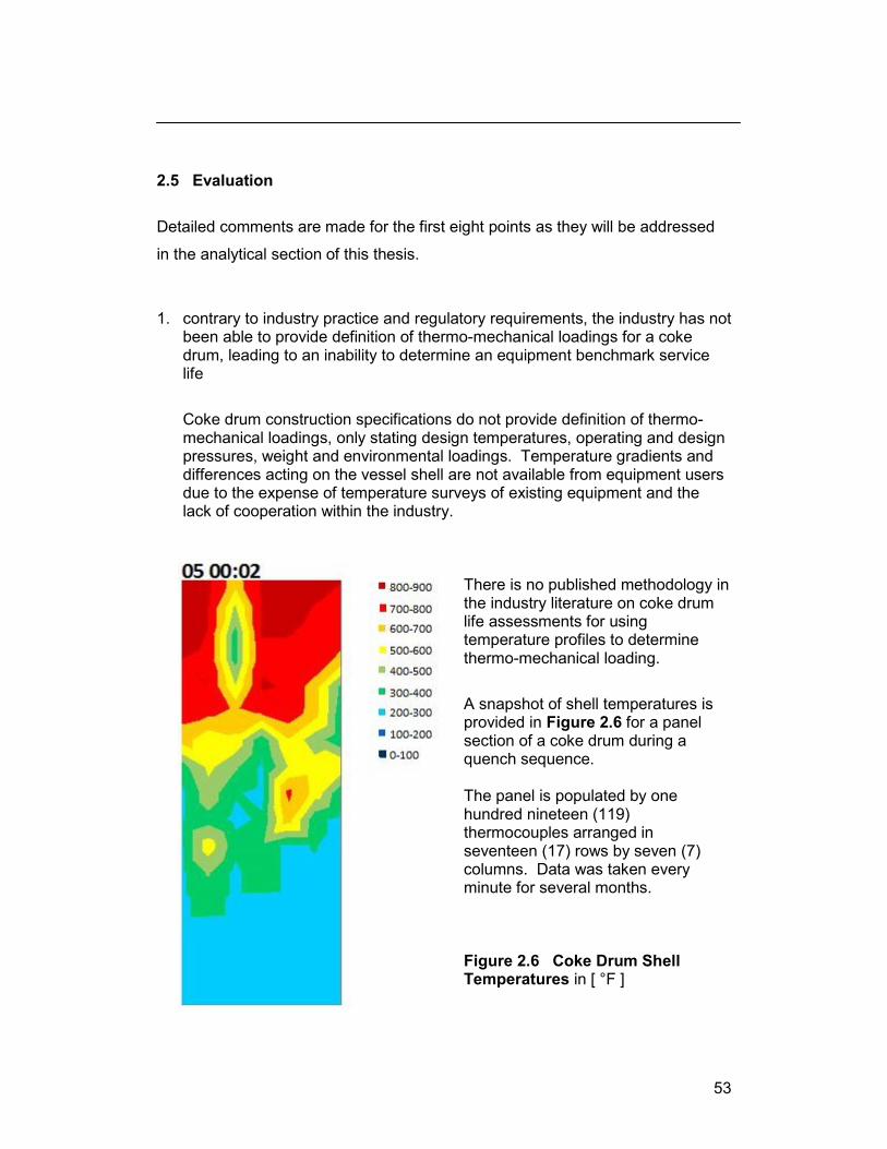
53

2.5 Evaluation

Detailed comments are made for the first eight points as they will be addressed

in the analytical section of this thesis.

1. contrary to industry practice and regulatory requirements, the industry has not

been able to provide definition of thermo-mechanical loadings for a coke drum, leading to an inability to determine an equipment benchmark service life

Coke drum construction specifications do not provide definition of thermo-mechanical loadings, only stating design temperatures, operating and design pressures, weight and environmental loadings. Temperature gradients and differences acting on the vessel shell are not available from equipment users due to the expense of temperature surveys of existing equipment and the lack of cooperation within the industry.

There is no published methodology in the industry literature on coke drum life assessments for using temperature profiles to determine thermo-mechanical loading.

A snapshot of shell temperatures is provided in Figure 2.6 for a panel section of a coke drum during a quench sequence. The panel is populated by one hundred nineteen (119) thermocouples arranged in seventeen (17) rows by seven (7) columns. Data was taken every minute for several months.

Figure 2.6 Coke Drum Shell Temperatures in [ °F ]

54

2. that fatigue assessments are made using material design fatigue curves rather than material service fatigue curves

The conventional practice has been to use the ASME VIII Division 2 fatigue strength data. Earlier editions of ASME VIII Division 2 ( prior to the 2007 edition ) used a design margin of 2.0 on stress / strain or 20 on cycles, whichever was more conservative at each data point [29], [30].

The margin on cycles was apportioned according to

2.0 for scatter of data

2.5 for size effect

4.0 for surface finish, environment

The most recent edition of the Code cites cyclic life values for smooth bar and weld joint specimens. The data for smooth bar specimens duplicates the life data provided in the earlier editions of the Code.

The design curves are provided on a material group basis, e.g. carbon steel, low alloy ferritic steel, stainless steel, high alloy versus individual material grades which obscures actual fatigue performance for a specific material.

Figure 2.7 shows the ASME fatigue design curve plotted against the data provided in Figure 2.4.

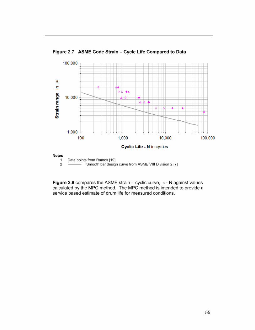
55

Figure 2.7 ASME Code Strain – Cycle Life Compared to Data

Notes

1 Data points from Ramos [19] 2 Smooth bar design curve from ASME VIII Division 2 [7]

Figure 2.8 compares the ASME strain – cyclic curve, - N against values calculated by the MPC method. The MPC method is intended to provide a service based estimate of drum life for measured conditions.

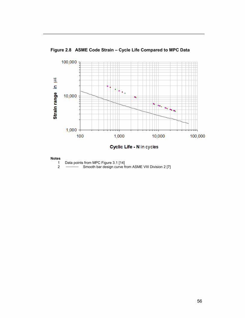
56

Figure 2.8 ASME Code Strain – Cycle Life Compared to MPC Data

Notes

1 Data points from MPC Figure 3.1 [14] 2 Smooth bar design curve from ASME VIII Division 2 [7]

57

3. that fatigue assessments are made with apparent incorrect determination of

strain ranges and counting of cyclic exposures

Strain ranges cited in all works are based on the measured strain range during an operational cycle. A strain gage can measure both compressive and tensile strains; for most of the strain exposures measured on the shell OD, the strain data shows the strain is either essentially tensile or compressive during the operational cycle.

Figure 2.9 shows strain profiles collected through five (5) operational cycles for three (3) strain gages mounted at the same elevation. Each operational cycle is about twenty four (24) hours in duration. The tracing spikes occur during the quench phase and display predominantly as either tensile or compressive strains and not as fully reversed strains.

The reported strain range is given as the range for each operational spike, only.

Consider the trace in Figure 2.9, a maximum tensile strain of 1,290 is

recorded in cycle 3, the minimum strain during the cycle is near 0 . In

cycle 4, a maximum tensile strain of 180 and minimum compressive strain

of 1,940 is experienced. A strain range of 1,940 is recorded for the operational cycle. However, the correct strain range for the two operational

cycles is 1,290 – (– 1,940 ) or 3,230 .

Figure 2.9 Strain Profile for Five Operational Cycles

Notes

1 Time scale reflects data from five operational cycles

58

The conventional nomenclature used by industry practitioners conflicts with Code convention. The Code provides the following definitions [7]:

Cycle – A cycle is a relationship between stress and strain that is established by the specified loading at a location in a vessel or component. More than one stress-strain cycle may be produced at a location, either within an event or in transition between two events, and the accumulated fatigue damage of the stress-strain cycles determines the adequacy for the specified operation at that location. This determination shall be made with respect to the stabilized stress-strain cycle.

Stress Cycle – A stress cycle is a condition in which the alternating stress difference goes from an initial value through an algebraic maximum value and an algebraic minimum value and then returns to the initial value. A single operational cycle may result in one or more stress cycles.

Operational Cycle – An operational cycle is defined as the initiation and establishment of new conditions followed by a return to the conditions that prevailed at the beginning of the cycle. Three types of operational cycles are considered:

1. the startup-shutdown cycle, defined as any cycle which has atmospheric temperature and/or pressure as one of its extremes and normal operating conditions as its other extreme;

2. the initiation of, and recovery from, any emergency or upset condition

or pressure test condition that shall be considered in the design; and 3. the normal operating cycle, defined as any cycle between startup and

shutdown which is required for the vessel to perform its intended purpose.

The nomenclature practice among equipment users is to designate the process operation illustrated in Figure 1.3 as an operational cycle.

Figure 2.10 illustrates the notion of the process operational cycle and Code practice operational cycle. Process operational cycle 3 displays an apparent

strain range of 1,290 while process operational cycle 4 displays an

apparent strain range of 1,940 . However, terminology consistent with

Code intent means that the strain range is 1,940 – (– 1,290) = 3,230 .

59

Figure 2.10 Notional versus Code Operational Cycle

The Code compliant cycle counting technique is performed by pairing sequentially the maximum peak to minimum valley strain values over all the operational cycles over the entire loading block. The loading block is the representative count of process operational cycles that precisely reflect the repetitive cyclic loading. In regards to the rainflow cycle counting technique, Collins advises [15]

“If cycles are to be counted over the duration of a duty cycle or mission profile block that is to be repeated block after block, the cycle counting should be started by initiating the first rain drop either at the most negative valley or the most positive peak, and continuing until all cycles in a complete block have been counted in sequence. This procedure assures that a complete strain cycle will be counted between the most positive peak and most negative valley in the block.”

This parallels the methodology of [7, 8] which reference the rainflow counting technique, Annex 5B paragraph 5.B.4 [7] and Annex B3 paragraph B3.4 [8]. A more intuitive and uncomplicated approach is recognized by both these industry documents as the “max / min” technique and follows discussion of the rainflow technique in those documents.

60

4. while temperature mapping of the coke drum is technically easy, use of these profiles has been not been effectively utilized

Samman states that “shell bulges and cracks could not be readily assessed using this industry standard [i.e., API 579 –1; author’s note ] because of the randomness and complexity of defining the cyclic thermo-mechanical loads that the shell experiences during operations” [26].

The MPC document reports that it uses the equipment users temperature or strain histogram when available [14]. The temperature histogram appears to be based on a concept of “thermal demand” wherein temperature gradients are determined to calculate a thermo-mechanical strain. Strain gages are used sparingly due to their cost and short time reliability.

Ramos noted the formation of cold spots but did not calculate thermo-mechanical strains using the temperature differences between shell locations and used strain gage readings [19]. Ramos used seventy five (75) thermocouples and six (6) strain gages over a grid of 2.7 m x 9.3 m.

This thesis uses the temperature readings directly to determine the thermo-mechanical strains. Good agreement is achieved by comparison to strain measurements.

61

5. the impact of the mismatch in the coefficient of thermal expansion between the clad liner (TP 410S stainless steel) and base material (C – ½ Mo, Cr – Mo) materials has not been generally recognized or used in fatigue assessments

Although the MPC recognized thermal mismatch between cladding and base material, an over simplified strain relation was provided

cladding = ( T operating – T ambient ) (2.5) To account for the expansion mismatch of both clad and base material , the following was established by Aumuller [31]; for the clad layer

1

1

1

)()( 0

bb

cc

chcb

c

Et

Et

ETT and, (2.6)

for the base layer

1

1

1

)()( 0

cc

bb

bhbcb

Et

Et

ETT (2.7)

Substitution with actual material property values indicates that the clad layer will be in tensile stress and the base material layer will be in compressive stress when the vessel is exposed to a temperature above reference (T0).

62

6. the trend in using higher yield strength Cr – Mo materials since the mid-1960’s has inadvertently resulted in drums being constructed from lower fatigue strength materials

Strong materials, i.e., materials with high monotonic yield strength have been shown to not necessarily possess high fracture ductility or fatigue strength. The concept is illustrated in Figure 2.11 showing that carbon and C – Mo have better low cycle fracture and fatigue strength in comparison to Cr – Mo low alloy steels currently favoured by equipment users [30], [32].

Figure 2.11 – N Fatigue Life for Pressure Vessel Steels

A combination of high plastic fatigue fracture ductility and fatigue strength over the cyclic life of interest, from start to 20,000 cycles, leads to the notion of relative fatigue toughness for C – Mo steels over Cr – Mo steels [33]. Original data, such as presented in Figures 2.12 – 2.17, indicates similar

trending but that strain exposure below 3,500 converges for the two materials with a slight advantage for C – Mo steels in TMF loading (Figure 2.13).

63

Table 2.1 quantifies the concept of ductility compared to material strength. C – ½ Mo is shown to have a higher proportional strain limit compared to Cr – Mo alloys except for 1 ¼ Cr – ½ Mo at 100 °F, only. In all other situations, C – ½ Mo is shown to have greater ductility. Since the materials undergo cyclic loading, it is necessary to consider the cyclic properties for a more accurate estimation of a cyclic elastic strain limit. This is addressed in Chapter 3.

Table 2.1 Monotonic Code Properties for Materials of Construction

SMYS SMTS E SMYS

[ ksi] [ ksi] [ 103 ksi ] [ ]

100 °F 900 °F 100 °F 900 °F 100 °F 900 °F 100 °F 900 °F

SA 240 405 25.0 16.9 60.0 44.0 29.0 23.2 0.086 0.073

SA 240 410S 30.0 20.3 60.0 44.0 29.0 23.2 0.103 0.088

SA 516 70 38.0 24.0 70.0 52.3 29.2 22.5 0.130 0.107

SA 204 C 43.0 30.0 75.0 69.7 28.9 22.2 0.149 0.135

SA 302 B 50.0 34.9 80.0 73.1 28.9 22.2 0.173 0.157

SA 302 C 50.0 34.9 80.0 73.1 28.9 22.2 0.173 0.157

SA 387 12 40.0 27.2 55.0 51.4 27.7 23.2 0.144 0.117

SA 387 11 45.0 30.6 60.0 55.8 27.7 23.2 0.162 0.132

SA 387 22 45.0 32.4 60.0 58.2 30.5 25.6 0.148 0.127

SA 387 21 45.0 32.4 60.0 58.2 30.5 25.6 0.148 0.127

Notes

1 SMYS, SMTS, E derived from reference [12]

2 Values of SMYS are calculated according to SMYS / E

64

Included in Table 2.1 is SA 302 C, a steel used in the nuclear industry where transient temperature loadings occur in certain equipment [34]. The nominal composition is described as Mn – ½ Mo – ½ Ni. Although SA 204 C is referenced conventionally as C – ½ Mo, its nominal composition is C – Mn – ½ Mo. Since SA 302 C has comparable carbon content the steels should be compared by nominal composition, as

SA 204 C C – 1 Mn – ½ Mo

SA 302 C C – 1½ Mn – ½ Mo – ½ Ni For high strain exposure, both of these low alloy steels have greater fatigue strength with SA 204 C showing improved ductility to SA 387 steels at ambient and high temperatures. SA 302 C shows markedly improved ductility to SA 204 C and SA 387 steels as an apparent result of increased Mn and Ni content. Fatigue strength testing shows C – ½ Mo steels with greater fatigue life than Cr – Mo steels below 10,000 cycles per Figure 2.12 [35]. These results occur under isothermal low cycle fatigue loading (ILCF).

Figure 2.12 Cycle Fatigue Life C – ½ Mo vs Cr – Mo at 900 °F [35]

65

In Figure 2.13, C – ½ Mo steels indicate consistently better fatigue life than Cr – Mo steels under low cycle thermo-mechanical fatigue loading (TMF) over an extended cyclic range. Figure 2.13 Cycle Fatigue Life C – ½ Mo vs Cr – Mo (TMF) [35]

7. weld fatigue strength and fatigue strength reduction has not been adequately

recognized

Weld fatigue strength is not accounted for in the MPC work. Up to the 2007 edition of the ASME Division 2 Code, weld fatigue strength was accounted for on the basis of a fatigue strength reduction factor to be applied by the practitioner. Values were typically 2 for butt welds based on learnings from related piping construction codes [36]. This is still a current practice [37]. Current industry practice using ASME VIII Division 2 and API 579 –1 / ASME FFS – 1 account for weld material explicitly using fatigue strength curves for weld joints Figure 2.14 compares the weld joint fatigue strength to the data of Ramos and Chen. It can be seen that the expected or average weld joint fatigue

strength is well below the measured data. The + 3 weld joint strength is just below the measured data which includes base and weld joint material.

66

Figure 2.14 Experimental Fatigue Strength vs ASME Code

Notes

1 ASME average fatigue curve, welded joint, 900 °F

2 ASME +3 fatigue curve, welded joint, 900 °F 3 Individual symbols are data from Ramos [19] and Chen [35]

67

The data from Ramos, shown in Figure 2.15 indicates lower fatigue strength for weld joints with very wide dispersion in the data.

Figure 2.15 Smooth Bar vs Welded Joint Fatigue Life, Ramos [19]

Notes 1 smooth bar data for SA 387 11, 850 °F 2 welded joint data for SA 387 11, 850 °F 3 Closed symbols for smooth bar data

4 Open symbols for welded joint data The data from Chen shows better correlation, Figure 2.16 and suggests a fatigue strength reduction of 1.1 to 1.3.

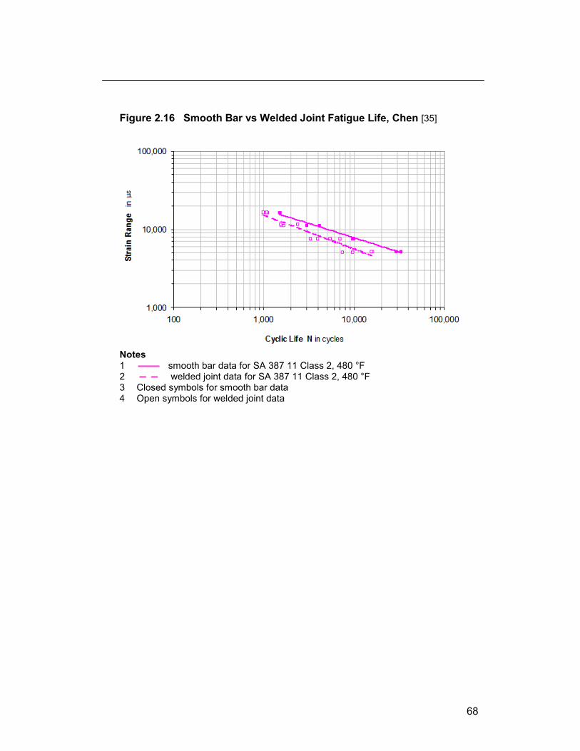
68

Figure 2.16 Smooth Bar vs Welded Joint Fatigue Life, Chen [35]

Notes 1 smooth bar data for SA 387 11 Class 2, 480 °F 2 welded joint data for SA 387 11 Class 2, 480 °F 3 Closed symbols for smooth bar data 4 Open symbols for welded joint data

69

8. that the dependence of fatigue strength reduction on the magnitude of strain / stress exposure is considered in industry practices, but is overly conservative

There are several items not well discussed in the literature

1. the dependence of fatigue strength reduction factor on strain 2. the fatigue strength reduction in the heat affected zone of the weld

joint 3. the dependence on both geometry and material property factors

The FSRF concept is discussed by Jaske in WRC 422 and notes clearly that the FSRF increases as strain range decreases, or conversely, as cyclic life increases [36].

Chen’s work is in agreement with Jaske but shows that the HAZ is more susceptible to fatigue strength reduction with the FSRF varying between 1.4 to 4.0 while the FSRF associated with weld failures varies between 1.6 and 2.1 [35].

The notion of fatigue strength reduction encompasses both a geometric component and a material property component and their interdependence.

Figure 2.17 presents the results of Chen’s work.

70

Figure 2.17 Smooth Bar, Welded Joint and HAZ Fatigue Life, Chen [35]

Notes

1 smooth bar data for SA 387 11 Class 2, 480 °F 2 welded joint data for SA 387 11 Class 2, 480 °F 3 HAZ data for SA 387 11 Class 2, 480 °F 4 Closed symbols for smooth bar data 5 Open symbols for welded joint, HAZ data

71

9. thermo-mechanical strain has not been explicitly addressed in coke drum design practice

The data, describing the magnitude and occurrence of thermo-mechanical strain, is not widely available in the open literature. Ramos et al. have published the results from their work and provided strain exposures and material fatigue charts [19]. Their effort focused solely on the skirt to shell junction. There are no published reports on how thermo-mechanical strains have been used explicitly for the design of coke drums. However, the principles are long established and industry practice documents are appropriate for implementation.

10. the impact of shell bulging is thought to be a hindrance for determining a

benchmark service fatigue life

Shell bulging has not been combined with thermal loading to determine impact on drum service life; note, however, that indirect measures have been presented in the literature. Finite element analysis of coke drums is performed and can account for shell distortions. A number of indirect measures have been used, but, have limitations and have not been validated.

11. thermal shock on surface strain development has been overlooked, the

magnitude of this strain matches the large strains developed from through thickness temperature gradients

There is published work on through thickness thermo-mechanical strain development in coke drums and link to drum cracking. It will be reviewed in the next section

12. drum operation is not adequately considerate of the impact of quench water

flow rates on the severity of thermomechanical loadings on the shell

A Unit Quench Factor was introduced early in the survey of coke drum operations but has not been developed since then. The use of fast quench water addition during a so-called proof quench was seen to be damaging.

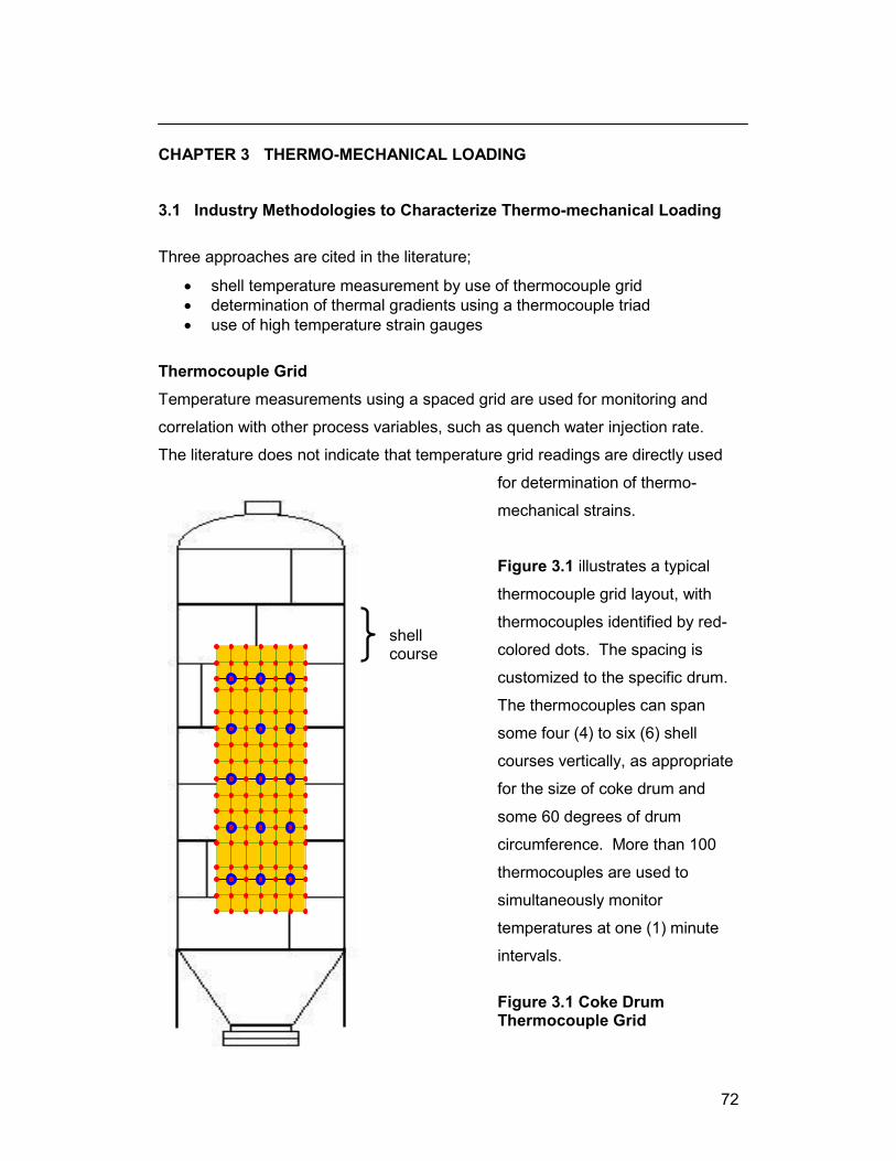
72

CHAPTER 3 THERMO-MECHANICAL LOADING

3.1 Industry Methodologies to Characterize Thermo-mechanical Loading

Three approaches are cited in the literature;

shell temperature measurement by use of thermocouple grid

determination of thermal gradients using a thermocouple triad

use of high temperature strain gauges

Thermocouple Grid

Temperature measurements using a spaced grid are used for monitoring and

correlation with other process variables, such as quench water injection rate.

The literature does not indicate that temperature grid readings are directly used

for determination of thermo-

mechanical strains.

Figure 3.1 illustrates a typical

thermocouple grid layout, with

thermocouples identified by red-

colored dots. The spacing is

customized to the specific drum.

The thermocouples can span

some four (4) to six (6) shell

courses vertically, as appropriate

for the size of coke drum and

some 60 degrees of drum

circumference. More than 100

thermocouples are used to

simultaneously monitor

temperatures at one (1) minute

intervals.

Figure 3.1 Coke Drum Thermocouple Grid

shell course

73

Thermocouple Triad

A thermocouple triad is intended to be used for determination of a thermal

gradient from which a thermo-mechanical strain is deduced. The triad consists of

three (3) thermocouples in axial and circumferential orientation at small spacing.

Figure 3.2 illustrates the thermocouple triad. The thermo-mechanical strain is

inferred by calibrating against strain gauges placed adjacent the thermocouple

triad.

The incentive to use this arrangement is the low cost of thermocouples and

relative reliability in a corrosive environment. However, the thermo-mechanical

strains determined by this arrangement are made by calibration of calculated

gradients with collocated strain gauges. An apparent weakness of the approach

is that the thermo-mechanical strain at a location does not depend uniquely on

local thermal gradients, only. Thermo-mechanical strains are seen to occur in

hot and cold spots where temperatures can be uniform and thermal gradients of

minor magnitude. The usefulness of temperature gradient measurements and

calculated thermo-mechanical strains is not discussed further in this thesis.

74

Figure 3.2 Thermocouple Triad for Measuring Temperature Gradient

In Figure 1.3, a temperature profile illustrated how a coke drum shell cools

nominally from bottom to top as

oil fill progresses through the oil fill cycle of several hours duration

quench water is rapidly added at completion of oil fill

Figure 3.3 shows the temperature response of another coke drum shell using

three (3) thermocouples; two (2) of which are located at the same elevation and

665 mm [26.1 “] apart along the circumference, the third thermocouple is located

3,119 mm [122.8 inches] below the other two. The temperatures are seen to be

nearly coincident during steam testing, vapor heating and the beginning of oil fill.

3” (75 mm)

3” (75 mm)

75

Figure 3.3 Coke Drum Temperature Profile during Operational Cycle

Similar to Figure 1.3, Figure 3.3 clearly indicates shell cooling begins

immediately as the oil fill level passes a thermocouple elevation but the large

time scale in Figure 3.3 erroneously suggests that the temperatures are uniform

during the water quench phase.

Using a smaller time scale in Figure 3.4 reveals the large differences in shell

temperature between the thermocouples at two different elevations (marked as

D3 – D8) and between two thermocouples at the same elevation (marked as C3

– D3). This more detailed view of thermocouple response reveals that the

cooling down of the coke drum shell is not uniform but that circumferential

gradients occur in addition to the expected axial gradients. This motivates the

inclusion of the thermocouple triad arrangements to determine the

circumferential, as well as the axial temperature gradients. This also shows the

motivation to examine temperature differences.

76

Figure 3.4 Thermocouple Readings in Detail

Notes

1 location D3, i.e., column D elevation 3 2 location C3, i.e., column C elevation 3 3 location D8, i.e., column D elevation 8 (a location 122.8 inches or

3,119 mm directly below elevation 3)

In a series of contour plots, the evolution of shell temperatures in four minute

intervals is shown in Figures 3.5a - l. The following observations can be made

from Figure 3.4 and Figures 3.5a – l

shell temperatures at a fixed location change rapidly, within about 15 to 25 minutes

both cold and hot temperature regions form during the quench sequence

cold spots can form spontaneously within an existing hot zone (Figures 3.5d – 3.5f; upper left quadrant)

cold intrusions or “fingers” can form by non-uniform upflow (Figures 3.5a – 3.5c)

the cold and hot regions may be extensive or localized

77

Figures 3.5 a – c Thermal Profile Snapshots – in [°F]

78

Figures 3.5 d – f (cont`d)

79

Figures 3.5 g – i (cont`d)

80

Figures 3.5 j – l (cont`d)

The extensive size of cold and hot spot regions jeopardizes a conventional

approach using only thermal gradients as a method to determine thermo-

mechanical strain.

While temperature gradients within the hot or cold spot may be relatively

small, large thermo-mechanical strains can be present since the affected cold or

hot spot is constrained by the surrounding structure. Zhang studied the impact

on coke drum shell strains in conditions of regional temperature differences [38].

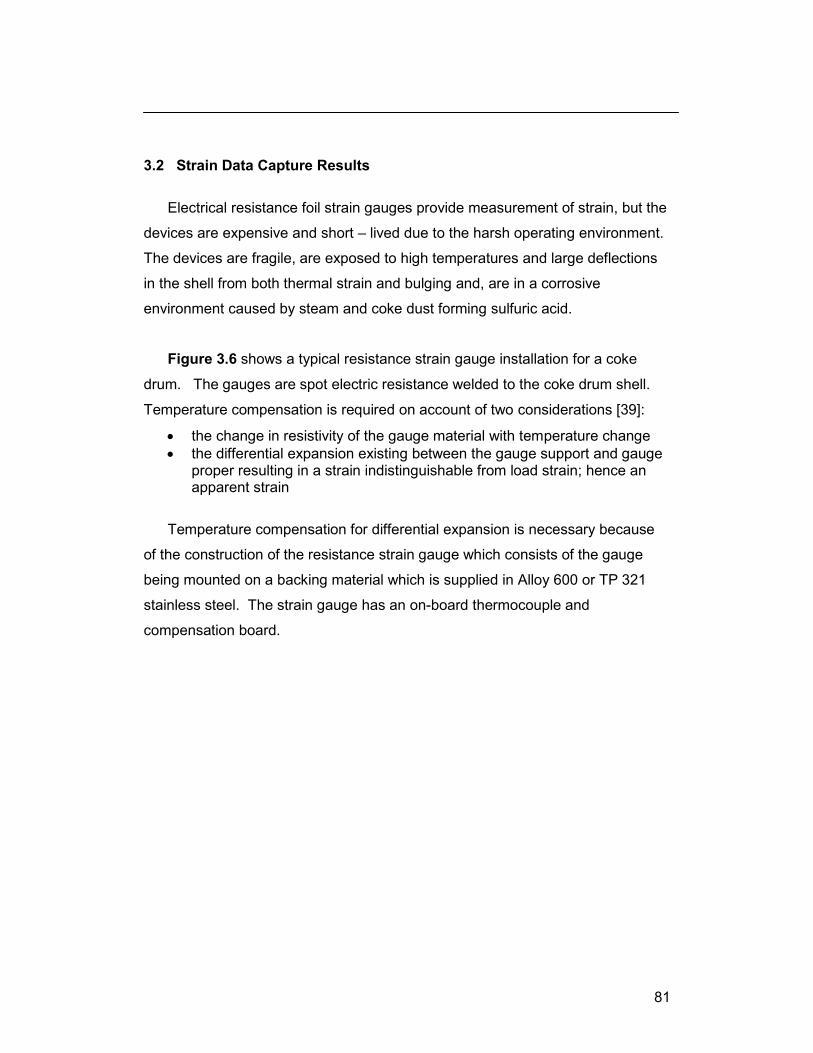
81

3.2 Strain Data Capture Results

Electrical resistance foil strain gauges provide measurement of strain, but the

devices are expensive and short – lived due to the harsh operating environment.

The devices are fragile, are exposed to high temperatures and large deflections

in the shell from both thermal strain and bulging and, are in a corrosive

environment caused by steam and coke dust forming sulfuric acid.

Figure 3.6 shows a typical resistance strain gauge installation for a coke

drum. The gauges are spot electric resistance welded to the coke drum shell.

Temperature compensation is required on account of two considerations [39]:

the change in resistivity of the gauge material with temperature change

the differential expansion existing between the gauge support and gauge proper resulting in a strain indistinguishable from load strain; hence an apparent strain

Temperature compensation for differential expansion is necessary because

of the construction of the resistance strain gauge which consists of the gauge

being mounted on a backing material which is supplied in Alloy 600 or TP 321

stainless steel. The strain gauge has an on-board thermocouple and

compensation board.

82

Figure 3.6 Strain Gauges with Independent Thermocouple

The temperature compensation circuit board is illustrated in Figure 3.7. The

strain gauge favoured by industry is usually a high temperature weldable unit

obtained from TML Tokyo Sokki Kenkyujo Type AWH [40].

An independent thermocouple arrangement is co-located and is identified by

the yellow and red leads suggesting that it is a Type “K” thermocouple.

83

Figure 3.7 Schematic of Strain Gauge and Compensation Board

A compensation scheme is provided and shown as Figure 3.8. The

manufacturer advises that the corrected strain is obtained as

corrected strain = measured strain – apparent strain (3.1)

Figure 3.8 Manufacturer`s Strain Gauge Compensation Chart

84

In Figure 3.9, the thermo-mechanical strain presented in equations (2.6) and

(2.7) are plotted.

Figure 3.9 Thermo-mechanical Strain due to CTE Mismatch

The expected strain at 900 °F [ 482 °C ] plots as a value of 2,215 for TP 410S

SS and – 244 for Cr – Mo steels. The strain plot is seen to continuously rise

for TP 410S and continuously decrease for Cr – Mo steels. In Figure 3.10, the

difference in thermo-mechanical strain reading between an Inconel backed

thermocouple and coke drum base material is shown. The thermocouple will

over-report the strain in the base by 1,240 at 900 °F [ 482 °C ], due to

differences in the coefficient of thermal expansion between the base material

and the thermocouple. The remaining error is attributable to the change in

resistance of the strain gauge and lead wire with temperature.

85

Figure 3.10 Thermo-mechanical Strain in Inconel Thermocouple Pad

The gauge manufacturer states that a corrected stress is provided through

this correction procedure and demonstrated by Figure 3.11 showing that

complete temperature compensation results in zero (0) strain indication due to

temperature and thermal strain induced by the differences in coefficients of

thermal expansion between the Type Alloy 600 gauge backing material and the

low alloy steel coke drum.

86

Figure 3.11 Strain Gauge Compensation [40]

87

6.85.28

5.28

9.27110.0

5.2811

)150()9.63.6(

,

1

1

1

)()( 0

b

cc

bb

bhbc

b

but

Et

Et

ETT

Strain History – Unit # 1

A strain tracing for an undisclosed coke drum shown in Figure 3.12 where D =

312 inches, t = 1 inch. Since the unit is pressurized during steam testing to 35

psig [241 kPag] and 250 °F [120°C], the calculated strains are:

1 = (1 – 2) / E (3.2) = (5,460 – 0.3 * 2,730) / 28.5

= 163 – circumferential

2 = (2 – 1) / E (3.3) = (2,730 – 0.3 * 5,460) / 28.0

= 38 – axial Accounting for the differential thermal expansion of clad to base materials, using

(2.6)

(3.4)

A difficulty with the strain history is correct interpretation of the operational

sequencing; the times for the transition in sequencing was not provided, hence

the analysis of strain gauge behavior is impaired.

88

Figure 3.12 Strain Profile #1

A decrease in thermo-mechanical strain is expected at the start of

sequencing since only pressure and temperature load are applied; i.e., 38 + (–

8.8) = 29 . This would persist until a hydrostatic head load occurs due to oil

filling. If the apparent strain gauge factor of – 175 is subtracted, then a

corrected strain of - 145 results and should be reported up to the start of

water quenching.

Two (2), of four (4) strain gauges installed on the coke drum shell show some

fidelity to the expected trend for pressure and steam heating. Given that a

compressive strain develops in the base layer due to the effect of internal

cladding, the strain should decrease slightly during vapor heating, from time

03:20 to 04:20 until the oil fill phase begins. A short time decrease is noted and

then oil filling begins at an unspecified time which could be also reported as

vapor heating.

89

889.25

9.25

9.25110.0

9.2511

)550()5.89.6(

,

1

1

1

)()( 0

b

cc

bb

bhbc

b

but

Et

Et

ETT

The phasing of operations is dependent on operator intervention and oil filling

could take place immediately after a short vapor heating phase.

Using the data from equation (1.1), the expected axial strain for combined

pressure and hydrostatic head (70 psig, 650 °F in this instance) is

1 = (1 – 2) / E (3.5) = (10,920 – 0.3 * 5,460) / 25.9

= 360 – circumferential

2 = (2 – 1) / E (3.6) = (5,460 – 0.3 * 10,920) / 25.9

= 84 – axial

A thermal strain of approximately – 88 is expected using (2.6).

(3.7)

The corrected axial strain is determined by (3.1) as

corrected strain = measured strain – apparent strain = [84 + (– 88) ] – (– 225)

= [– 44] + 225 = 180

The reported strain (i.e., strain gauge plot) should be then calculated as a

corrected strain of 180 . The plotted strains in Figure 3.12 vary between

approximately 500 and 600 with average coker drum shell temperature at

650 °F [ 343 °C ].

90

Note that the black colored tracing is for a strain gauge located at the skirt which

is subject to shell wall cooling which initiates early in the oil filling sequence.

Thus, the strain gauges mounted on the shell read higher than expected and

are not consistent with the pressure and final live weight loading in the coke

drum. A maximum reading of 1,250 - axial is reported in this operational cycle

which occurred during the quench phase of operations; during the quench phase,

coker drum shell temperature decreases as quench water is added to the coke

drum. This strain development is representative of additional observations over

a block of eighteen (18) days.

Strain History - Unit # 2

The strain history for a second coke drum unit was examined for comparison.

Figure 3.13 shows the circumferential strains for several strain gauges and

temperature (the temperature is shown in gray and uses the left hand scale)

collocated at one of the gauges.

Figure 3.13 Circumferential Strain Profile # 2 for Five Operational Cycles

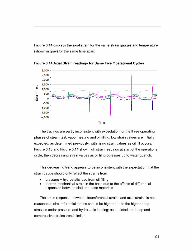
91

Figure 3.14 displays the axial strain for the same strain gauges and temperature

(shown in gray) for the same time span.

Figure 3.14 Axial Strain readings for Same Five Operational Cycles

The tracings are partly inconsistent with expectation for the three operating

phases of steam test, vapor heating and oil filling; low strain values are initially

expected, as determined previously, with rising strain values as oil fill occurs.

Figure 3.13 and Figure 3.14 show high strain readings at start of the operational

cycle, then decreasing strain values as oil fill progresses up to water quench.

This decreasing trend appears to be inconsistent with the expectation that the

strain gauge should only reflect the strains from

pressure + hydrostatic load from oil filling

thermo-mechanical strain in the base due to the effects of differential expansion between clad and base materials

The strain response between circumferential strains and axial strains is not

reasonable; circumferential strains should be higher due to the higher hoop

stresses under pressure and hydrostatic loading; as depicted, the hoop and

compressive strains trend similar.

92

However, all tracings are consistent in showing that the highest strains

occur during the water quench phase, only

are of short duration

are an order of magnitude larger during the quench phase than strains measured during the other phases of operation

are within the elastic strain limit of the materials and within the shakedown limit of 2· YS provided in the Codes

Overall, the strain tracings for Unit # 2 are not fully consistent with expected

response of the temperature compensated strain gauges.

3.3 Discussion of Measured Strains

These tracings indicate that the correct observation of strain using high

temperature strain gauges under high temperature conditions is problematic.

1. In the available reports, the validation of the reported strain gauges reading is not provided.

2. The accuracy of strain gauge reading is not established; there is no discussion to verify the readings

The elastic strain limits given in Table 2.1 were presented on the basis of

Code specified minimum yield strength properties [ SMYS ].

However, the elastic limit values provided in Table 3.1 are determined on the

basis of actual supplied yield strength [ YS ] properties. The SMYS is a Code

requirement while YS values are the actual monotonic yield strength

properties for the supplied material.

Figure 3.15 shows the results from a monotonic tensile test of a 2¼ Cr - 1

Mo used for construction of a coke drum.

93

Figure 3.15 Monotonic Stress – Strain Curve for 2¼ Cr – 1 Mo Material

The Code SMYS, defined as the 0.2% offset strength is shown to be 67,116

psi [462.7 MPa]. The actual extension under load [EUL] of the test piece is

0.423%. The proportional limit is determined with strain at 0.2% EUL and tensile

stress at 60,810 psi [419.3 MPa] resulting in a Young’s modulus of 30.6 E6 psi

[210.7 GPa]. The supporting MTR for this specimen cited the material as SA 387

22 Class I. The elastic limit in Table 3.1 is 2,190 at 100 °F [38 °C]. It should

be noted that yield strength may be stated on the basis of 0.2% offset or 0.5%

EUL [41].

94

Table 3.1 Actual Material Properties for Coke Drum Construction

Material

YS TS E YS

100 °F 900 °F 100 °F 900 °F 100 °F 900 °F 100 °F 900 °F

SA 240 405 29.0 23.2

SA 240 410S 29.0 23.2

SA 516 70 29.2 22.5

SA 204 C 56.0 35.9* 81.0 75.3 28.9 22.2 1,940 1,620*

SA 302 B 56.3 39.3* 83.7 - 28.9 22.2 1,950 1,770*

SA 387 12 – II 63.1 42.9* 83.5 - 27.7 23.2 2,280 1,850

61.5 41.8* 80.5 - 2,220 1,800

65.9 44.8* 84.1 - 2,380 1,930

65.7 44.7* 82.7 - 2,370 1,925

60.8 41.3* 79.6 - 2,195 1,780

SA 387 11 – I 59.0 40.1* 76.3 - 27.7 23.2 2,130 1,725*

56.0 38.0* 76.5 - 2,020 1,640*

60.2 40.9* 78.7 - 2,170 1,765*

57.2 38.9* 77.2 - 2,065 1,675*

60.0 40.8* 80.4 - 2,165 1,760*

SA 387 22 – I 38.1 27.4* 69.3 - 30.5 25.6 1,250 1,070*

40.9 29.4* 70.2 - 1,340 1,150*

SA 387 22 – II test

67.1 48.3* 83.1 - 30.6 25.6* 2,190 1,885

SA 387 21 30.5 25.6

Notes

1. * indicates value is estimated from MTR and Code data

2. elastic strain limit YS calculated according to YS / E

3. stress values in ksi; strain values in

95

SA 387 / Cr – Mo materials are routinely specified in the Class II condition

resulting in higher monotonic strength properties. The grade 11 and 12 Cr – Mo

materials, i.e., 1¼ Cr – ½ Mo and 1Cr – ½ Mo were supplied in both Class I and

Class II condition. However, the actual measured monotonic elastic strain limits

are well above the measured coke drum shell strains for Unit # 1 and for four of

five strain excursions shown for Unit # 2. The maximum excursion for Unit # 2 is

within the 2 · YS / E limit.

The monotonic elastic strain limits are summarized in Table 3.2 for SA 387 [Cr –

Mo] materials.

Table 3.2 Monotonic Elastic Strain Limits for SA 387 Materials – in YS / E 2 · YS / E

100 °F 900 °F 100 °F 900 °F

SA 387 12 – II 2,195 2,380 1,780 1,930 4,390 4,760 3,560 3,860

SA 387 11 – I 2,020 2,170 1,640 1,760 4,040 4,340 3,280 3,520

SA 387 22 - test - 2,190 - 1,885 - 4,380 - 3,770

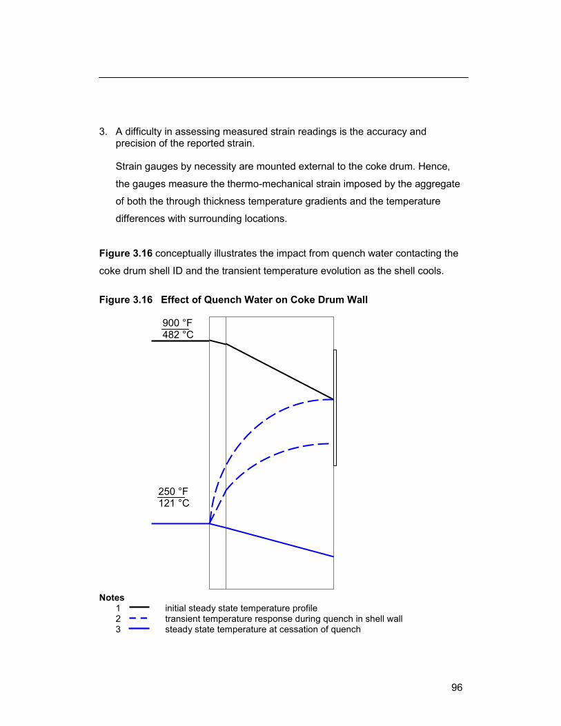
96

250 °F 121 °C

900 °F 482 °C

3. A difficulty in assessing measured strain readings is the accuracy and precision of the reported strain. Strain gauges by necessity are mounted external to the coke drum. Hence,

the gauges measure the thermo-mechanical strain imposed by the aggregate

of both the through thickness temperature gradients and the temperature

differences with surrounding locations.

Figure 3.16 conceptually illustrates the impact from quench water contacting the

coke drum shell ID and the transient temperature evolution as the shell cools.

Figure 3.16 Effect of Quench Water on Coke Drum Wall Notes

1 initial steady state temperature profile 2 transient temperature response during quench in shell wall 3 steady state temperature at cessation of quench

97

Some industry researchers have investigated the effects on heat transfer rate

from quench water to coke drum shell ID and quench water rise rate on shell

distortion (bulging) and plastic strain development [24][25]. Ohata concludes

from transient thermal and strain analysis that the maximum strains approach

0.2% plastic strain, Figure 3.17.

Figure 3.17 Equivalent Plastic Strain in Coke Drum Wall

A bounding approach based on the model of Figure 3.16 suggests that the

total bounding strain could be calculated as [33]

615,4250900101.7T 6 (4.8)

The bounding model is overly-conservative since it presumes that the coolest

possible water temperature contacts the hottest coke drum shell region

instantaneously and is completely encircled by the hot zone. This strain value,

consisting of elastic and plastic components aligns with Ohata’s assumptions.

98

The actual heat transfer rate is limited by the surface boiling conductance.

Aumuller determined surface conductance during water quench and suggested a

limit value of 1,280 W / m2 - °C [225.6 Btu / hr – ft2 - °F] [31].

Ohata et al. indicate that when using a surface boiling conductance of 1,200

W / m2 - °K and a fast water rise rate, the equivalent plastic strain developed in

their model was zero (0); Figure 3.18 is provided from the reference [24].

Figure 3.18 Plastic Strain Development during Likely Water Quench

Ohata et al. used the 0.2% yield strength criterion to determine the elastic strain

limit for their model. Their model used an isotropic hardening model, cycling

loading was not used. Ohata does not report the actual proportional limit strain;

however, using experimental data by the author, this could coincide with a

proportional strain limit of 0.213%. Figure 3.19 presents results from room

temperature monotonic testing of 1¼ Cr – ½ Mo pressure vessel construction

material similarly specified by Ohata.

99

Figure 3.19 Monotonic Stress Strain Curve for 1¼ Cr – ½ Mo

Figure 3.20 presents another strain histogram from a coker drum which is

consistent with the expected strain history behaviors described above for Unit # 1

and Unit # 2:

mechanical strain readings are near zero (0) during oil fill since only thermal strains are present; thermal strains cause zero thermo-mechanical strains

a small negative strain reading occurs due to differential thermal

expansion between clad and base material; this is about – 200 and somewhat consistent with calculation (3.7)

strain readings rise linearly when the oil fill elevation exceeds the strain gauge elevation, somewhat consistent with calculation (3.6)

a negative strain spike occurs of approximately – 2,000 consistent with quench water contacting the shell ID; a rapid shell temperature decline from 720 °F [ 382 °C] to 250 °F [121 °C] occurring in 15 minutes.

100

Figure 3.20 Operational Data from Coke Drum

Summarizing from the Ohata study

a room termperature monotonic elastic strain limit using the 0.2% offset strength was used

strains do not exceed elastic strain limits for realistic heat transfer rates during water quenching, i.e., 1,280 W / m2 – °C [225.6 Btu / hr – ft2 - °F]

Strain readings for surface mounted strain gauges, as applied to coke drums,

can occur from several sources

through thickness temperature differences

temperature gradients between shell locations

temperature differences between shell locations

101

3.4 Interpretation of Strain Data

Strain data are necessary to determine the cyclic life of coke drums exposed

to thermomechanical loadings using the – N approach.

The strain measurements captured by strain measurement gauges from the

available literature and industry partner were examined. These are given in

Figures 3.21a through 3.21d.

Figure 3.21a Strain Gauge Data Distributions from the Literature – # 1

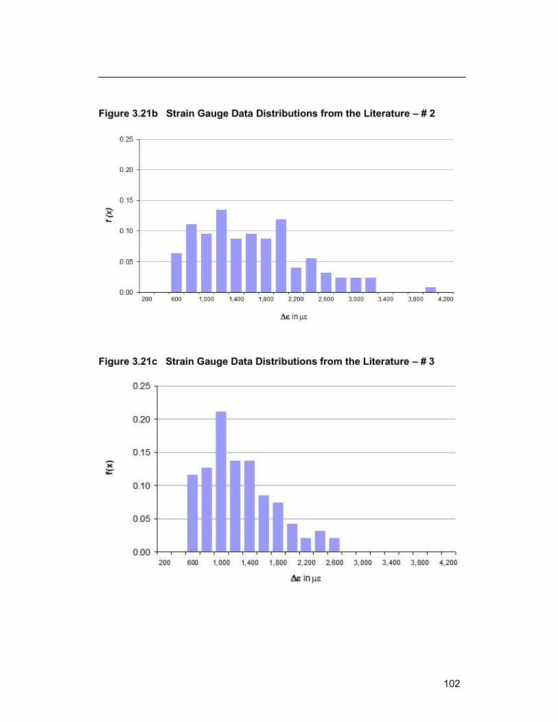
102

Figure 3.21b Strain Gauge Data Distributions from the Literature – # 2

Figure 3.21c Strain Gauge Data Distributions from the Literature – # 3

103

Figure 3.21d Strain Gauge Data Distributions from the Literature – # 4

For convenience, the four (4) strain signatures are collated and displayed in

Figure 3.22 and labeled # 1 to # 4. Data set # 4 is taken from the open

literature.

Figure 3.22 Collated Strain Distributions

104

The individual strain results for each location are combined to form a single

distribution and shown in Figure 3.23 for purposes of statistical characterization.

An average strain range of 1,190 , and variation of +1 = 590 was

calculated. This indicates that nearly 90% of the strains as reported by the

industry occur within the monotonic 1 · YS / E strain limit.

Figure 3.23 Aggregated Strain Distributions

Using Table 3.3; only 1 of 458 readings, i.e., 0.2% of the data is outside of

the

2 · YS / E strain equivalent shakedown limit stipulated by Code criteria. An

upper temperature limit of 650 °F is used to correspond to the upper temperature

limit experienced under quench conditions.

105

Table 3.3 Monotonic Elastic Strain Limits SA 387 Materials, 650 °F in

YS / E 2 · YS / E

100 °F 650 °F 100 °F 650 °F

SA 387 12 – II 2,195 2,380 1,910 2,071 4,390 4,760 3,819 4,141

SA 387 11 – I 2,020 2,170 1,759 1,888 4,040 4,340 3,518 3,776

SA 387 22 - test - 2,190 - 1,980 - 4,380 - 3,961

The cyclic stress – strain curve for 1¼ Cr – ½ Mo coke drum shell material

shown in Figure 3.24 shows that the elastic strain range in cyclic loading is

approximately 4,600 which exceeds the strain distributions summarized in

Figure 3.23. Hence, the strain exposures in coke drums under

thermomechanical loading are likely all in the cyclic elastic strain range.

Figure 3.24 Cyclic Stress – Strain Curve for SA 387 Grade 11 Material

106

CHAPTER 4 FATIGUE LIFE CRITERIA

The ASME Code limits design fatigue life by stipulating an allowable number

of cycles for the stress or strain experienced by a component. The basis of the

ASME fatigue curves is based on a phenomenological treatment of fatigue which

spans both the high cycle and low cycle regimes comprising mechanical fatigue.

The current industry Code, ASME VIII Division 2 provides a combined stress

based criteria and using a pseudo-elastic stress criteria for the low cycle portion

of the normally referenced S – N curve. The curves are particularized for

material groups and operating temperature to a maximum component

temperature of 700 °F [371 °C]. This temperature limit is based on creep

considerations; but, in practice the curves are used above this temperature and

are extrapolated using the methodology available within the Code rules.

4.1 Criteria of the ASME Code

The origin of low cycle fatigue curves derived with the separate works of

Coffin and Manson [42] and, Manson [43] ] in the 1950’s who proposed a low

cycle fatigue curve using two monotonic properties; ultimate tensile strength and

reduction of area. The ASME Code simplified this, as explained by Langer

building on the work of Coffin [see [ref 7] in Langer paper [44] ] to present the

following development [44, 45]:

107

Referencing Coffin (LF Coffin, A Study of the Effects of Cyclic Thermal Stresses

on a Ductile Metal”, Trans. ASME Vol 67, 1945) [45, 46]

(4.1) (4.2) (4.3) (4.4)

Since the Code was intended to be applicable to high cycle fatigue, as well,

strain was converted to a linearized stress expression, as

(4.5)

The expression, Se was set at the endurance limit and an error of 16% was

estimated at N = 1,000 cycles. This provided for a continuous curve spanning

both the low cycle ( < 105 ) and higher cycle portions ( > 105 ) to use in pressure

vessel construction.

e

ep

p

f

ff

p

RAN

RAN

henceRA

eec

where

cN

100

100ln

2

11

100

100ln

2

11

100

100ln

2

1

then, Since

i.e. fracture, at strain true or ductility fracture the ;

t

t

e

e

SRAN

RANS

2100

100ln

2

11

100

100ln

2

11

E

EE E2 t

108

Langer shows the development to the more recognizable form using

Manson’s approach by partitioning the phenomenological expression into a

plastic range and an elastic range by letting

(4.6) (4.7) (4.8)

(4.9)

Hence, the coefficient “z” in (4.7) is – 0.5 using Coffins approach.

Manson showed that the coefficients “k” and “z” can be determined from a

minimum of two (2) strain – fatigue tests at well-separated values of strain to

observe S and N. Manson tested a number of materials, Figure 4.1 and

presented universal slope values to be used for estimates for cyclic life when the

complication of an assumption of the exponents as a material property was not

warranted [43].

5.21

2

1

,,5.21

100

100ln

2

1

2

t

kf

f

kf

kz

t

k

e

z

p

NEN

e

asorNENRA

and

GNMN

then

GNSandMN

109

Figure 4.1 Strain versus Cyclic Life [43]

The values of – 0.12 for the elastic component and – 0.6 for the plastic

component were recommended as indicated in Figure 4.2.

Figure 4.2 Coffin – Manson Universal Slopes Approach [42]

110

Hence, (4.10)

Later, Manson and Hirschberg presented a modification [47]

(4.11)

Manson stipulated that the Universal Slopes Equation was not intended for

use with specific materials; rather, if specific materials were tested the

appropriate material properties would need to be established and substituted into

equation (4.7).

Manson later explained the difference between his formulation, which used

an exponent of - 0.6 for low cycle fatigue, to the value of the exponent of - 0.5 in

Coffin’s formulation.

ASME VIII Division 2 adopted the Manson expression using an exponent of –

0.5 and explicitly provides the development of the Code basis in reference [48].

This is a key document in understanding and using the Code.

The ASME Code prescribes the design fatigue curve provided in Figure 4.3.

Carbon, low alloy steels and TP 4xx, low chrome stainless steels are grouped in

the design fatigue curve which may be particularized using the specific Young’s

modulus value at temperature. The ASME design curve is developed from

smooth bar test specimens and presented as a pseudo-elastic stress amplitude.

t012.06.0 5.2

2

1 NE

Nf

f

t012.06.0

6.0

5.3100

100ln

N

EN

RA

u

111

Figure 4.3 Fatigue Design Curve Prescribed by ASME VIII Division 2

Notes:

1. Stress amplitude – N curve from ASME VIII Division 2, as published prior to the 2007 edition

Both elastic – structural stress analysis and elastic – plastic analysis

approaches are allowed. A structural stress range is employed for the former

and an equivalent structural stress is employed for the latter. The structural

stress is a function of the membrane and bending stresses normal to the

hypothetical crack plane and modified for low cycle fatigue using Neuber’s rule

[48].

The smooth bar fatigue design curve is consistent with Code practice from

introduction of the 1st edition of ASME VIII Division 2 in 1963 and up to the

edition released in 2004. The approach to determination of the fatigue life of

welds was to use a fatigue strength reduction factor applied to the elastically

calculated stress. For full penetration butt welds, as used to join pressure vessel

shell sections, this was taken as two (2) to 2.5. The factor was applied by

multiplying the calculated stress amplitude by 2 to 2.5 prior to entering the fatigue

design curve.

112

Jaske presented data showing that non-isothermal thermo-mechanical

fatigue are much more damaging to fatigue strength than isothermal strain

cycling [49, 50]. Figure 4.4 – is reprinted from Figure 3 from STP 770, with

clean up of data at 800 °F for AISI 1010 carbon steel. The results from in –

phase and out – of – phase thermo-mechanical loading was shown to be both

more deleterious than isothermal fatigue.

Figure 4.4 Comparison of Thermo-mechanical to Isothermal Fatigue [49]

A clean sheet rewrite of the Code was released in 2007 which introduced a separate curve for the design fatigue assessment of welded joints based on use of elastic – structural stress analysis. The release has not addressed Jaske’s concerns about non-isothermal strain cycling. There are several important considerations in using the Code fatigue design curves for the purpose of determining a service fatigue life for coke drums.

113

Three considerations are listed

1. the curves are design curves intended for the design life estimation of pressure vessel components in fatigue service. By using a design margin, use of the Code curve ensures safe operation of the pressure vessel throughout the design life by providing an alert point

2. the extent of failure is not specified within the Code; the Code does not state the failure criterion in establishing fatigue failure, namely, whether complete through thickness separation or incipient cracking

3. the applicability to non-isothermal strain cycling

4.2 ASME Design Fatigue Life Margins

The ASME design fatigue curves are intended to determine a design life. In

comparison, the notion of service life for a pressure vessel is defined to be the

reasonably expected life in service under actual service conditions rather than

design operating conditions. The Code design life definition includes margins to

account for uncertainty in determination of service loads as well as crack

initiation or fracture.

The design approach is a combined approach using the following:

1. Equipment owners add a small margin to the maximum temperature and

pressure loads expected in service 2. The Code mandates a design margin on the use of the allowable stress to

be used for the determination of the pressure thickness by equation (1.1). The allowable stress, S is based on the lower of

2/3 · SMYS, or

1/3.5 · SMTS at the design temperature.

114

Since most pressure vessel construction materials are supplied to a higher

quality than stipulated by the Code, additional margins are provided implicitly.

Tables 2.1 and 3.1 demonstrate the difference between Code minimum strength

requirements and material measured strengths.

For a coke drum, the design margins on pressure and temperature are

verified by review of the design specification sheet provided by the equipment

owner. For example, the CRD partner coke drums have a declared design

temperature of 925 °F [496 °C], but operated well below this temperature at 700

°F [371 °C](Fig 4.23) for a long period prior to temperatures rising to more

modern targets of 850 °F [454 °C] to 900°F [482 °C]

Figure 4.5 plots the ASME smooth bar design curve for the material group

including carbon, low alloy and TP 4xx stainless steels adjusted to 900 °F [482

°C] against the experimental data of Ramos and Chen.

115

Figure 4.5 Comparison of ASME Smooth Bar Design to Measured Data

Notes

1 smooth bar design curve for ferritic steel material category – [900 °F] 2 Closed symbols for smooth bar experimental data 3 Open symbols for welded joint, HAZ experimental data

The design margin for the ASME smooth bar design curves is 20:1 on cycles

and 2:1 on stress / strain [30, 36].

Figure 4.6 plots the (1) ASME design curve, (2) the curve based on use of

the 20:1 factor applied to cycles and, (3) the curve based on the 2:1 factor

applied to strain, with all three curves corrected to 900 °F [482 °C]. The curves

are plotted against the data from Ramos for 1Cr – ½ Mo and 1¼ Cr – ½ Mo

steels tested at 850 °F [454 °C] and the data from Chen at 900 °F [482 °C]. The

plot indicates that the design margin of 20:1 on cycles is appropriate at low

cycles to approximately 50,000 cycles and confirms the disclosure in references

[30, 36]. Here, Barsom and Vecchio advise that the fatigue design curves were

obtained from mean curves by applying a factor of 20 on cycles and 2 on stress

and using the more conservative resulting value. The factor of 20 prevailed in

the low-cycle regime (i.e., below about 10,000 cycles). The presented plot,

Figure 4.6 indicates differences consistent with the ASME methodology.

116

Figure 4.6 ASME Fatigue Curve Design Margins

Notes

1 welded joint design curve for ferritic steel material category – [900 °F] 2 design curve multiplied by 20 on cycles 3 design curve multiplied by 2 on stress 4 Closed symbols for smooth bar data 5 Open symbols for welded joint, HAZ data

For the clean sheet rewrite of the Code, ASME included a welded joint design

curve with confidence intervals for ±1± 2 and ± 3 standard deviations. The

welded joint design curve and the +3 curve at 900 °F [482 °F] are plotted

against the Ramos and Chen data in Figure 4.7. The +3 welded joint curve

plots at the lower bound of the experimental data and suggests a bounding limit

for C – ½ Mo and Cr – Mo alloys that are used for coke drum fabrication.

117

Figure 4.7 ASME Design Curve with + 3 Confidence Interval

Notes

1 welded joint design curve for ferritic steel material category

2 + 3 confidence interval 3 Closed symbols for smooth bar data 4 Open symbols for welded joint, HAZ data

Note that for the design of welded joints, the ASME Code prescribes the use

of a lower bound welded joint design curve of – 3limited to 700 °F (ref: ASME

D2 par #.F.2.2(a)). The work of Ramos and Chen show that the fatigue strength

fatigue curves can be extended to 900 °F [19, 35]. It is not known whether the

welded joint fatigue curves are overly conservative since the experimental data is

not available to the public.

118

4.3 Code Fatigue Failure Defined

The Code does not describe the anticipated failure mode being protected

against; i.e., crack initiation or specimen separation.

Manson studied both crack initiation and crack fracture and noted the

ambiguity in the literature. However, he did show that an exponent of – 0.5 for

the plastic strain range aligned with crack initiation. Crack initiation was defined

to be the number of cycles to initiate a 0.003 inch [0.080 mm] deep crack in a ¼“

[6.35 mm] diameter fatigue specimen. Failure life, Nf was defined to be the

number of cycles to separate the specimen [48, 51, 52].

Kalnins established independently that Code failure corresponds to

observation of a small crack of 0.5 mm [0.020 inch] in fatigue specimens and not

crack propagation through the thickness [53]. Another key observation is that

geometries which possess a uniform strain through their thickness will behave

consistent with Code rules. Hence, the fatigue models were indicative of

membrane strains (i.e., low cycle fatigue) and membrane stresses (i.e., high

cycle fatigue).

The Code assesses crack propagation using fracture mechanics approaches

in order to predict final failure i.e., separation of components. However, for the

determination of service fatigue life for coke drum service, this effort uses the

definition of fatigue failure as implicitly practiced by the Code because

coke drum thicknesses vary according to pressure thickness criteria

the specific environmental factors present in a coke drum and their impact on crack propagation are not established

use of the initiation criterion provides a level of conservatism

119

4.4 Non- Isothermal Loading

Jaske showed that non-isothermal loading was more damaging than

isothermal loading for AISI 1010 carbon steel [49]. Chen shows that the fatigue

life of C – ½ Mo and Cr – Mo steels is comparable under either loading condition

at high strain but a significant benefit is observed with C – ½ Mo at the lower

portion of the strain levels used in the study [35].

Chen felt that thermo-mechanical fatigue testing simulated the thermal and

mechanical loading conditions experienced by coke drums [35].

The operational sequencing of a coke drum is illustrated in more detail in

Figure 4.8. The temperature and pressure scales are intentionally not plotted.

1. pressure loading occurs at the start of the production cycle and remains nominally constant throughout the oil filling cycle

2. steam heating occurs simultaneously as pressure loading 3. a vapor heat up occurs in follow up to the steam heat / pressure loading 4. oil filling commences after steam heating and vapor heating 5. hydrostatic loading from live weight loading occurs under isothermal

conditions 6. on completion of oil filling, water quenching is initiated; thermo-mechanical

strains occur under isothermal and non-isothermal conditions depending on whether “hot spots” or “cold spots” develop

Large compressive strains occur during nominally isothermal conditions when “hot spots” form. For “cold spots”, large tensile strains form under in-phase non-isothermal conditions since they are related to non-uniform contact of quench water with the shell.

120

Figure 4.8 Sequencing of Coke Drum Operational Cycle

Notes

1 CS 4 refers to temperature evolution at shell course 4 2 CS 5 refers to temperature evolution at shell course 5 3 pressure evolution in coke drum 4 vapour heat, oil fill and quench time spans as indicated

For determination of a service fatigue life, a reasonably conservative

approach is needed but with less conservatism than used by the Code design

fatigue life methodology.

This is complicated by the behavior of so-called “strong” materials,

exemplified by Cr – Mo steels (SA 387 22), and ductile materials, such as the C –

½ Mo and C – Mn – Mo or Ni steels (SA 204 / SA 302). Figure 4.9 shows the

iso-thermal, low cycle fatigue (ILCF) behavior and non-isothermal, thermo-

mechanical (TMF) behavior of the two steels over the low cycle range of the

strain – fatigue life curve. For the C – ½ Mo steels, the ILCF curve is more

conservative in the range of interest [35].

121

The operating temperature is specific to the equipment and may be in a

temperature range extending from 650 °F to 900 °F [343 °C to 482 °C]. For this

work, a temperature of 900 °F [482 °C] will be used for convenience.

Particularization to specific units is necessary for application to actual coke

drums.

Figure 4.9 Fatigue Life Comparison of Strong versus Ductile Materials

Notes 1 LCF means isothermal low cycle strain fatigue testing 2 TMF means in-phase thermal and strain fatigue testing

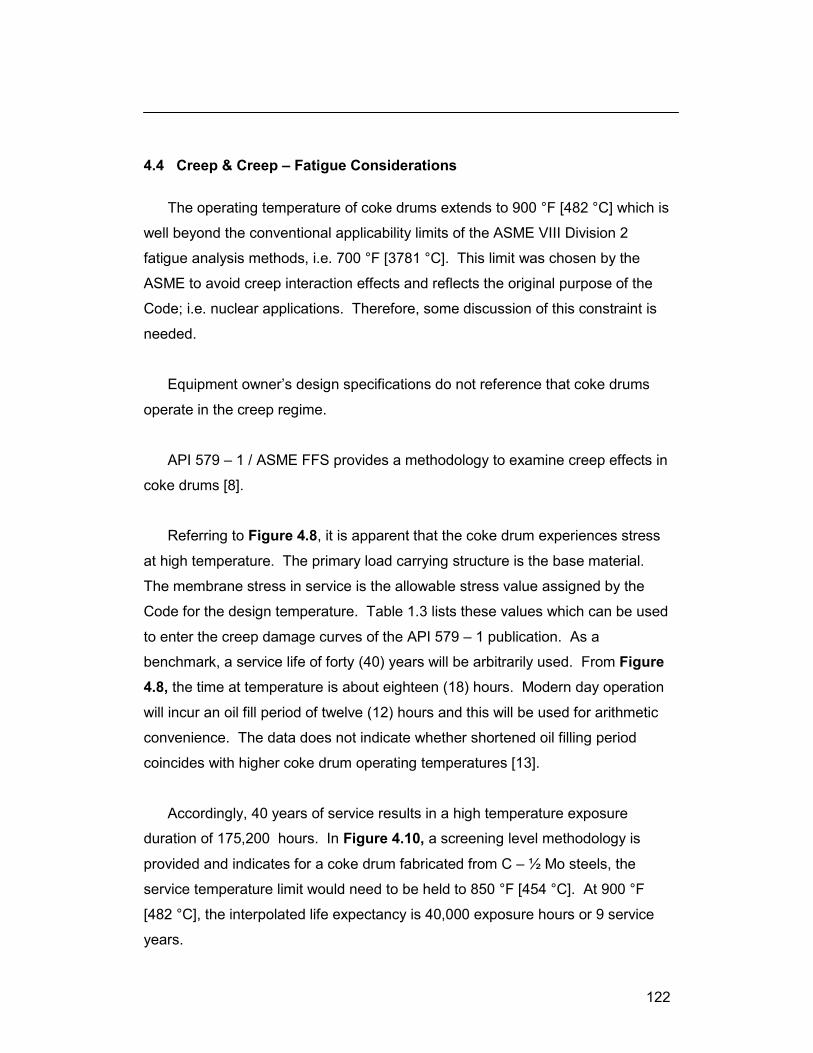
122

4.4 Creep & Creep – Fatigue Considerations

The operating temperature of coke drums extends to 900 °F [482 °C] which is

well beyond the conventional applicability limits of the ASME VIII Division 2

fatigue analysis methods, i.e. 700 °F [3781 °C]. This limit was chosen by the

ASME to avoid creep interaction effects and reflects the original purpose of the

Code; i.e. nuclear applications. Therefore, some discussion of this constraint is

needed.

Equipment owner’s design specifications do not reference that coke drums

operate in the creep regime.

API 579 – 1 / ASME FFS provides a methodology to examine creep effects in

coke drums [8].

Referring to Figure 4.8, it is apparent that the coke drum experiences stress

at high temperature. The primary load carrying structure is the base material.

The membrane stress in service is the allowable stress value assigned by the

Code for the design temperature. Table 1.3 lists these values which can be used

to enter the creep damage curves of the API 579 – 1 publication. As a

benchmark, a service life of forty (40) years will be arbitrarily used. From Figure

4.8, the time at temperature is about eighteen (18) hours. Modern day operation

will incur an oil fill period of twelve (12) hours and this will be used for arithmetic

convenience. The data does not indicate whether shortened oil filling period

coincides with higher coke drum operating temperatures [13].

Accordingly, 40 years of service results in a high temperature exposure

duration of 175,200 hours. In Figure 4.10, a screening level methodology is

provided and indicates for a coke drum fabricated from C – ½ Mo steels, the

service temperature limit would need to be held to 850 °F [454 °C]. At 900 °F

[482 °C], the interpolated life expectancy is 40,000 exposure hours or 9 service

years.

123

Figure 4.10 ASME Level 1 Creep Screening Criteria for C – ½ Mo

Notes

1 Open symbol plots operation of interest in Figures 5.10 – 5.12

For 1¼ Cr – ½ Mo steels, using Figure 4.11, the anticipated life 140,600 hours.

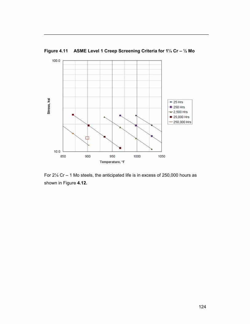
124

Figure 4.11 ASME Level 1 Creep Screening Criteria for 1¼ Cr – ½ Mo

For 2¼ Cr – 1 Mo steels, the anticipated life is in excess of 250,000 hours as

shown in Figure 4.12.

125

psi 615,673.01

1

1

2.23

8.241

2.23110.01

)900()2.71.9(

1

1

1

)()( 0

c

bb

cc

chcbc

Et

Et

ETT

Figure 4.12 ASME Level 1 Creep Screening Criteria for 2¼ Cr – 1 Mo

For the TP410S clad layer, differential thermal expansion at service temperature

results in a pseudo – elastic stress of

(4.11)

126

Entering Figure 4.13 from API 579 – 1, the stress load exceeds the

screening level criterion and creep cracking is to be expected. A detailed study

by Penso et al. of the metallurgical condition of a coke drum found extensive

cracking in the clad material. The most prevalent cracking was shallow, “spread

on the entire internal surface in all samples analyzed” with average depth of 1

mm. Cracks of greater depth occurred in the fusion boundaries of clad and clad

weld [20]. The 1996 API survey reported that 64% of survey respondents

reported ID initiated cracking while 71% reported OD initiated cracking [sic] [13].

The survey did not clarify how ID to OD crack initiation was established.

Figure 4.13 ASME Level 1 Creep Screening Criteria for 12 Cr / TP410S

127

u

mean

alt

eq

S

S

SS

1

4.5 Fatigue Curves

The numerous fatigue studies available in the open literature allow

determination of a specific fatigue curve for the materials of construction of coke

drums. The design fatigue curves in the industry standard literature, however,

are not sufficiently detailed.

4.6 Mean Strain Effects

Mean strain effects are acknowledged by the ASME criteria but are stated to

be inconsequential for low and medium-strength materials and no adjustment for

mean stress is necessary where stress reaches yield strength. Hence, for low

cycle fatigue, mean stress effects are not required [48].

In contrast, O’ Donnell states, in the ASME Companion Guide, that mean

stress effects necessitate determination of an equivalent alternating stress

component prior to entering the fatigue life curve [54]. He refers to use of the

modified Goodman diagram or use of the closed form expression

(4.12) where

Seq ≡ equivalent alternating stress amplitude to enter the S – N graph Salt ≡ apparent alternating stress amplitude Smean ≡ mean stress Su ≡ ultimate tensile strength

Collins provides data showing that mean strain effects are negligible from

Nf = 100 to chart end at Nf = 10,000 cycles i.e., the low-cycle range according to

Figure 14.4 [15].

128

Figure 4.14 Impact of Mean Strain on Fatigue Life, Collins [15]

Alternatively, Stephens, Fatemi et. al present data which suggests mean strain

(stress) does have influence in the low cycle fatigue life range, Figure 4.15 [55].

Figure 4.15 Impact of Mean Strain on Fatigue Life; Stephens, Fatemi [55]

Notes

1. For SAE 1045 low carbon steel, hardened

129

cff

bf

mfa NN

E

22

2

''

Stephens, Fatemi et al. argue that because of stress relaxation at large strain

amplitudes due to the presence of plastic deformation, mean stress effects on

fatigue life is small in the low-cycle fatigue region.

Reference is made to “Morrow’s mean stress method” in which the strain

amplitude,

(4.13)

is adjusted by inclusion of the m term in the elastic portion of the Basquin

equation, refer to equation (2.1). This follows the trend displayed in Figure 4.15

which applies to a high carbon content plain carbon steel, while it is inconsistent

with the data of Figure 4.14 which is for an aluminum alloy.

130

CHAPTER 5 ANALYSIS OF COKE DRUM THERMO-MECHANICAL STRAINS

Strains may be obtained directly from an operational drum using high

temperature strain gauges, as discussed in § 3.2. Strain gauges are used

sparingly, though, in practice due to

their high unit cost

limited operating life

inaccuracies and improper use

The operating life for strain gauges is limited due to

the large, imposed thermal strains

their mechanical fragility in comparison to the imposed strains

high operating temperatures

corrosive environment

The accuracy and precision of strain gauges has not been investigated for

this work and has not been demonstrated in the available literature as previously

discussed in § 3.2. A more robust approach is provided by the use of

thermocouples.

In Figure 3.1, 15 strain gauges and 119 thermocouples are used in the test

panel. Strain gauge locations are represented by blue circles enclosing the red-

colored dots representing thermocouple locations. As seen in Figures 3.6 and

3.7, the thermocouple is much simpler, consisting of thermocouple wire requiring

only spot welding to the pressure vessel shell. When damaged in service, the

thermocouple can be quickly repaired and reattached with small effort. The

existing wire can be reused and reattached by trimming the corroded portion

attaching to the shell. A recent design practice by equipment users is to use

replaceable insulation panels on the shell that allow quick access to the shell

surface.

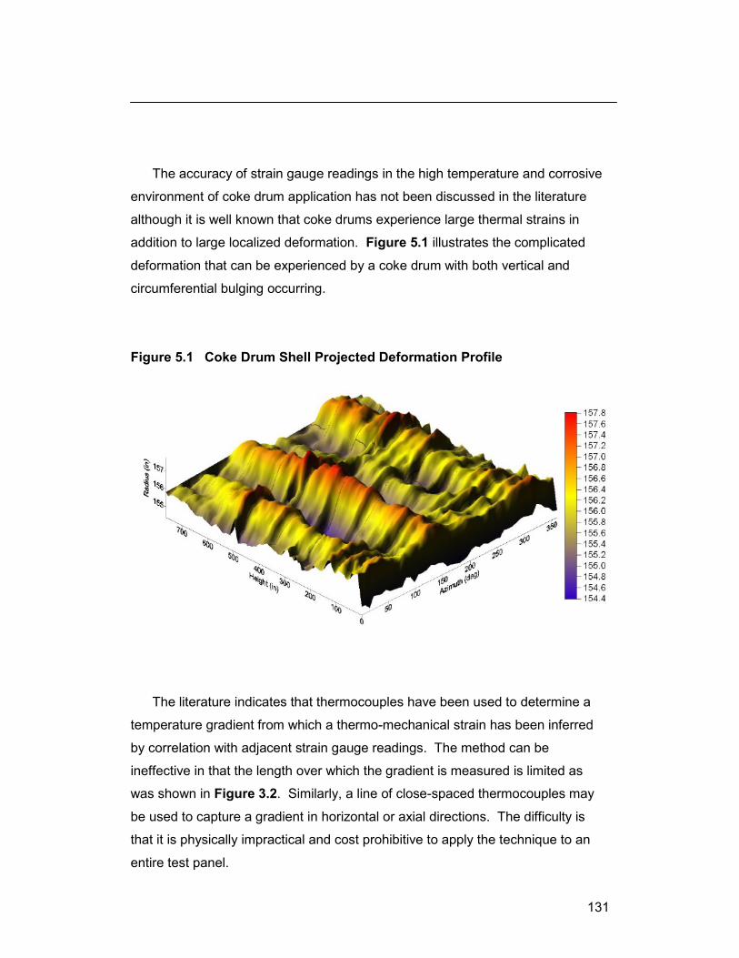
131

The accuracy of strain gauge readings in the high temperature and corrosive

environment of coke drum application has not been discussed in the literature

although it is well known that coke drums experience large thermal strains in

addition to large localized deformation. Figure 5.1 illustrates the complicated

deformation that can be experienced by a coke drum with both vertical and

circumferential bulging occurring.

Figure 5.1 Coke Drum Shell Projected Deformation Profile

The literature indicates that thermocouples have been used to determine a

temperature gradient from which a thermo-mechanical strain has been inferred

by correlation with adjacent strain gauge readings. The method can be

ineffective in that the length over which the gradient is measured is limited as

was shown in Figure 3.2. Similarly, a line of close-spaced thermocouples may

be used to capture a gradient in horizontal or axial directions. The difficulty is

that it is physically impractical and cost prohibitive to apply the technique to an

entire test panel.

132

The temperature gradients inferred from the tightly spaced grid do not

necessarily correlate with strain gauges which will also include thermo-

mechanical strains from more extensive effects, not only local temperature

gradients. The practice has been to space the grids on approximately 1 inch

centers over a single 2 foot length arc and vertical cross. Additionally, the data

from this arrangement has not been made available in the industry literature.

Temperature data can be inexpensively obtained during coke drum operation

over an extensive area and extended time period by use of simple thermocouple

devices as pictured in Figure 3.6.

133

5.1 Temperature Based Life Estimate Methodology

The objective of this thesis is to estimate a service life based on temperature

data since this data can be more simply and reliably retrieved. The essential

steps in considering and accomplishing this are

to retrieve temperature data for a suitable grid over a statistically relevant period

that actual drum temperature data is used; this has been provided by a confidential source which logged temperature data at one-minute intervals for a one-year period

that data from 51 or more consecutive cycles is taken; a block of 52 operating cycles was used

that the temperature readings be interpolated in order to provide suitable input for determination of corresponding thermo-mechanical strains; an appropriate interpolation scheme must be established

to assign the interpolated temperatures to a corresponding finite element grid to calculate the associated thermo-mechanical strains

to repeat the process for an appropriate interval during the significant portion of the water quench cycle; this is the portion of the operating cycle which contains the maximum strain response

to assemble the maximum and minimum strain exposures established for an individual water quench cycle

to assemble the exposures from successive operational cycles as a block strain exposure profile and make a numerical count of maximum / minimum counts consistent with industry methodology

to make a life estimate consistent with the precision stated in § 1.2

134

Temperature Evolution During Water Quench

In Figures 3.5a – l, a sequence of snapshots demonstrate the evolution of

temperatures for a thermocouple grid presented in Figure 3.1 during the water

quench phase for an operational cycle. The grid spacing is approximately 665

mm [26.181”] horizontal and varying in the vertical direction between 570 mm

[22.4”] and 683 mm [26.890”]. Spacing variations are due to field obstructions.

Figure 3.5g is reproduced as Figure 5.2 with grid lines whose intersections

represent the thermocouples.

Figure 5.2 Detailed Thermal Snapshot Profile, Part Grid 04 23:58

135

Table 5.1 lists the associated temperature readings for each of the grid points for comparison to Figure 5.1.

Table 5.1 Local Grid Temperature Readings for Figure 5.1 Row

822 817 694 813 826 821 817 1

814 806 544 803 821 816 802 2

818 802 511 802 821 819 809 3

804 797 509 790 812 812 771 4

800 803 739 807 812 806 665 5

784 762 695 758 791 787 546 6

S1 S2 S3 S4 S5 S6 S7

Column

Figure 5.3 details the local temperature distribution as presented by data

display software at grid point 4 – S3 where a low temperature of 509 °F is

measured. Temperature gradations are easily seen to be linear along the

horizontal and vertical grid lines.

Figure 5.3 Local Thermal Snapshot Profile, Part Grid 04 23:58

136

The physical distance between data points is large, nominally on the order of

665 mm [26”] and is too coarse to provide a valid FEA input mesh for calculation

of thermo-mechanical strains.

There is no data available in the industry literature on coke drum temperature

surveys to provide insight to the temperature distribution between discrete data

points. The same situation applies to strain data recovered at discrete data

points; only fifteen (15) strain gauged data points were provided among one

hundred nineteen (119) thermocouple data points presented in Figure 3.1.

Heuristic Temperature Interpolation

Review of multiple temperature histograms such as depicted in Figures 3.5a

– l show similar behaviors during water quenching;

coke drum temperatures decrease in a nominally axisymmetric pattern in the bottom shell courses; this is consistent with the expected uniform rise in the level of water and consequent uniform decrease in shell temperature from bottom to top

as water fill progresses into the cylindrical section, channeling occurs between the coke bed and coke drum shell and present as periodic intrusions (“fingers”) as exemplified in Figure 3.5b

as internal channeling allows water to migrate into the higher temperature parts of the coke bed and, consequently, horizontal water flow makes contact with the coke drum shell, cold spots form above the nominal water level as revealed in Figure 3.5c - f

the cold spots span a shorter distance circumferentially (3 consecutive t/c locations), but span a longer distance vertically (6 consecutive t/c locations), Figure 3.5h is presented as Figure 5.3 with grid markings, the intersections of the grid markings are t/c

hot spots can span both small and large distances; the larger hot spots occur in the upper portions of the coke drum shell, while smaller hot spots occur in lower and upper portions; Figure 5.4. Note that this thermal profile is the interpolated linear profile from the captured (i.e., as measured) field data.

137

Hot spots occur where portions of the coke drum shell are protected from

contact with water by, ostensibly, tightly adhering coke; eventually this effect

dissipates as water eventually fills and soaks the interior of the coke drum.

Figure 5.4 Thermal Snapshot Profile, Measured Full Grid 05 00:06 in [º F]

138

A number of interpolation schemes may be considered to model the

temperature gradient between thermocouple locations; Kreith presents solutions

to analogous situations such as [56]

the temperature profile of the billet undergoing rapid heat transfer; the billet is initially at a uniform temperature and subjected to rapid cooling during the quenching bath. The temperature distribution, subject to Newtonian cooling, is expressed as a negative exponential relationship

for an extended surface under forced convection, the temperature distribution along its length is given by:

(5.1)

T ≡ temperatature along the extended surface Ts ≡ temperature at base of extended surface

T ≡ temperature at end of extended surface

x ≡ distance along the extended surface m ≡ characteristic geometry and heat transfer properties of the

extended surface

The solution is given in the form: (5.2) for which the solution in simplified dimensionless form becomes

(5.3)

The parameter “m” effectively constrains the quantity ( TTi ) between sT and

T by setting “m” to 1; the quantities sT and T are the bounding temperatures.

The usual application of this expression in heat transfer problems uses a

calculated value of “m” in order to establish a predicted value of iT along L up to

the end of the extended surface T , which for infinitely long surfaces may be the

ambient temperature.

mxmx eCeCTT

21

whereTTmdx

Td 2

2

2

mL

xLmTTTT i

sicosh

cosh

139

In this case, T bounds the end temperature limit for a finite length surface.

Simple plotting for values of “m” in equation (5.3), to compare the numerator to

denominator of the hyperbolic cosine terms, readily reveals this bounding

behaviour.

Thus, Kreith’s approach suggests an interpolation function in final form such

as

(5.4)

where, fTT ,0 are the measured temperatures at the boundary points, Ti the

interpolated temperature at distance xi , L being the distance between the

boundary points. The use of an interpolation scheme is heuristic since the

transient temperatures at intervening locations are not measured and are likely

as random as the measurements at the thermocouple locations; accordingly,

other interpolation schemes could be explored that may be more convenient or

simpler.

Data for the coker drum is provided at one-minute intervals, hence the coke

drum surface temperature distributions are posed as successive realizations and

result in recovery of a spectrum exposure profile.

Figure 5.5 displays the exponential interpolation of temperature locally in the

vicinity of the cool spot for the full grid profile presented in Figure 5.4. The

profile extends across the full width of the panel and for the top six (6) rows. At

intersection points, temperatures match exactly the measured data points.

LxL

TTTT iffi

cosh

cosh0

140

Figure 5.5 Local Interpolation of Thermal Snapshot Profile in [º F]

In Figure 5.6, a simple comparison is made between the measured data and

the linearly interpolated and exponentially interpolated local temperatures. The

exponentially interpolated data can be seen to impose a more severe gradient

with the expected increased severity in thermo-mechanical strain.

141

Figure 5.6 Local Interpolation of Thermal Snapshot Profile

142

5.2 Schema for Strain Determination

To determine the mechanical strain generated by the temperature differences

indicated by the data, a finite element analysis is made. The considerations in

developing the models are

the most simplified model that accurately estimates the thermo-mechanical strains should be used; testing models of varying sophistication and complexity may be required

repetitive modeling will be required in order to establish the thermo-mechanical strain evolution throughout the water quench period for each operational cycle

the FEA model will not require consideration of time dependent effects, coke drum materials are selected to avoid creep, by specification and demonstrated in §5.4; but, should address temperature dependent material properties, as warranted

the finite element model should be simple and efficacious to alleviate computational effort and minimize error potential in recognition of practices by industrial end users; the simplifying practices of the nuclear industry should be considered in execution of FEA approaches

the coke drum shell is composed of a clad and base layer; a composite shell element is desirable but will be limited to linear analysis due to the underlying application of composite shell FEA modeling and software limitations

analysis is made using a hierarchy of effort; the simplest approach is made initially, more sophisticated approaches are made consequently as demonstrated by need; this is consistent with industrial practices and practices in the nuclear industry [54]

data is available at one-minute intervals; for 119 t/c grid points and 271 operational cycles results in 2 to 3 million data points to be processed to isolate the thermo-mechanical strains; to manage this large data base a sampling approach is used which truncates the number of data points to 42 t/c grid points over 52 cycles at four-minute intervals resulting in a sample data load of 34,000 to 51,000 data points

the temperature interpolation of these data points results in a data load of 3 to 5 million data points for execution of the FEA modeling for 42 t/c grid points and 52 operational cycles

143

a sufficient number of temperature snapshots (these are at one minute intervals) need to be processed to identify the maximum thermo-mechanical strain and strain range during the operational cycle

the maximum and minimum mechanical strain values for an operational cycle are then isolated

the consecutive maximum and minimum pairing of strain values for an operational block are isolated to establish the mechanical strain exposure for the loading block

the loading block is the representative loading exposure for the grid and is representative of the repeated thermo-mechanical loading for the coke drum over its service life

accounting for the loading effects of pressure, live weight and deadweight loads (§ 1.6) is specifically disregarded due to their marginal contribution as demonstrated by both Aumuller and Chen [32, 34]; this brings focus onto the impact of the thermo-mechanical loading

144

5.3 Service Life Estimate Schema

The maximum / minimum pairing of strain values defines the thermo-

mechanical strain signature for the loading block and provides the data for

establishing the damage accumulation. The calculation process is outlined;

for a fixed location, list the maximum, max and minimum, min thermo-mechanical strain determined in an operational cycle

list the maximum, max,i and minimum, min,i thermo-mechanical strains determined for the 52 operational cycles / loading block

rearrange in order to pair each maximum strain with each minimum thermo-mechanical strain, in succession, for the loading block to define the thermo-

mechanical strain range signature, k = [max,i - min,i]k

for each strain range pairing, enter the service strain – life graph and determine the damage fraction for the strain range pair, uk = nk / Nk

sum the damage fractions, U = uk for the loading block

determine the service life

145

5.4 Defining a 1st Pass Finite Element Model

The 1st pass model presents a reasonably simplified model consistent with

industrial and nuclear industry practices; this includes

use of a composite shell element to distinguish clad and base layer construction

partially dependent temperature; use respective material properties at 650 °F; for coke drums, final operating metal temperatures vary according to specific installation and operational requirements; this temperature is a sufficiently conservative and practical 1st pass choice

truncated shell section

4 minute snap shot intervals

cylindrical coordinate system; Z (vertical), R (radial), T (circumferential); (NB: occasionally, T is assigned the label Y)

material of construction is taken as SA 204C for the base layer, TP 410S stainless for clad layer; these are typical materials used in the industry

thickness is 1 inch [25.4 mm] thick for the base layer, ⅛ “ [3.2 mm] for the clad layer; the thickness for the base layer is consistent with conventional construction Code rules which take into account specific mechanical loads, temperature and material selection;

the radius for the shell model is taken from incidental information taken from the temperature data base; coke drums have radius dimensions determined by specific production requirements and hence, will vary from installation to installation

pressure loading is not applied for two reasons

to isolate the thermo-mechanical loading

it does not materially affect calculation of the strain range in the loading

block and entry in the strain – life ( – N) curve on account of its small value

for information,

the mechanical strain occasioned by pressure loading is only

approximately 0.000186 or 186 and thermo-mechanical loadings

exceed a range of 5,000 (demonstrated later); hence, any impact is not distinguishable given the accuracy in service life fatigue life data

146

The model is presented in Figure 5.7.

Figure 5.7 1st Pass FEA Model

Z

t

r

RT, RR = 0 UZ is coupled in UZ

RT, RZ = 0 UT = 0

RT, RZ = 0 UT = 0

RT, RR = 0 UZ = 0

X ≡ location of node N1861

147

Notes to Figure 5.7 1. The element used for the model is the SHELL4L 4-node multi-layer quadrilateral shell

element with

membrane and bending capabilities for the analysis of three-dimensional structural and thermal models

up to 50 layers can be used; 2 layers are used for this analysis

six degrees of freedom (3 translations and 3 rotations) are considered per node

one degree of freedom per node representing the temperature is used in the thermal analysis

each layer can be associated with different isotropic or orthotropic material properties; isotropic material behaviour is used for the model

2. UZ, UR, UT ≡ translational displacement; RZ, RR, RT ≡ rotational displacement; in the cylindrical coordinate system

3. The top edge of the model is coupled / constrained to preserve plane-remains-plane boundary condition; this ensures no node can displace axially relative to other nodes

4. No displacement occurs acriss tge circumferential boundaries 5. Radial displacement is unconstrained 6. Dimensional information for the panel, the panel comprises a 60° arc of a cylinder

with the following attributes; mean radius 150 inches [3,810 mm] thickness of base layer 1 inch [ 25.4 mm] thickness of clad layer 0.118 inch [ 3 mm] height 290 inches [7,366 mm]

7. Uniform mesh size is used without localized mesh refinement since the undamaged surface is uniform

8. Software used:

COSMOSM™ Version 2.8, Structural Research & Analysis Corporation, Los Angeles, CA

COSMOSM™ Version 2010, SolidWorks 2011 Simulation, Dassault Systèmes SolidWorks Corporation, Waltham, MA

Structural Research and Analysis Corporation [SRAC] was founded in 1982 by Dr. Victor I. Weingarten, Department of Civil Engineering at the University of Southern California, Los Angeles. It was acquired in 2001 by Dassault Systems S.A.

148

Temperature Interpolation; In reference to the finite element model proposed

in Figure 5.7 above, the explicitly marked node points (small circle, symbolized

by ○) are the forty two (42) node points at which measured temperature is

provided in a data set that was recorded for 52 operational cycles at one minute

intervals. This results in a data set of 60,480 (42 x 60 x 24) data points for each

cycle, (3,145,400 data points for 52 cycles). In order to determine the thermo-

mechanical strains, a structural analysis, using temperatures from intermediate

data points are needed. These temperatures are interpolated using a specific

scheme based on heat transfer considerations as suggested by expression (5.4).

Accordingly, from forty – two (42) measured temperature points, a total of

3,069 (i.e., 3,111 – 42) interpolated temperature data points are established to

form the input to the thermo-mechanical analysis; these input data points form

the thermal snapshot (i.e., the temperature status is available for each minute of

the operational cycles but, four (4) minute intervals are used to reduce the data

management effort.

149

5.5 Evolution of the Thermo-mechanical Strain Profile

Temperature loading of the coke drum shell results in thermal expansion of

the shell; the shell expanding in height and diameter by virtue of the increase in

temperature during the various temperature increases caused by operation.

These are

steam test phase; T is from ambient to steam test temperature, 100 °F to 250 °F [38 °C to 121 °C]

vapor heating phase; T is from 250 °F to 600 °F [121 °C to 316 °C]

oil fill phase; T is from 600 °F to 900 °F [316 °C to 482 °C]

Thermo-mechanical strains arise due to the differential heating of the shell

and, also, from differences in the coefficient of thermal expansion (CTE) of clad

and base layers. The effect of CTE has been addressed by the presented

equations.

During steam testing and vapor heating phases, the coke drum is empty and

all parts of the coke drum are exposed to temperature increases uniformly, as

evidenced by the data.

To isolate the effects of differential temperature exposure over a coke drum

shell, consider a drum shell with only one type of material, thereby, no CTE effect

occurs and the following expressions apply:

150

The total strain developed in the shell is expressed by

(5.5)

for which,

thermal = ∙T i.e., coefficient of expansion x the temperature difference

thus,

mech = 0 when only thermal loading is present, and

total = thermal for steam test and vapor heat phases (5.6)

and, as already indicated, the mechanical strain, mech , developed from pressure

and hydrostatic loads is included during the operational cycle.

During the water quench phase, uneven cooling results and the posed single

layer coke drum shell is no longer unconstrained resulting in development of a

mechanical strain from self constraint from by differential temperatures; in the

following, there are no external mechanical loads and hence,

(5.7)

The temperature distribution for a specific snapshot is shown in Figure 5.8.

T

thusand

thermalmech

thermalmech

thermalmechtotal

,0

thermalmechtotal

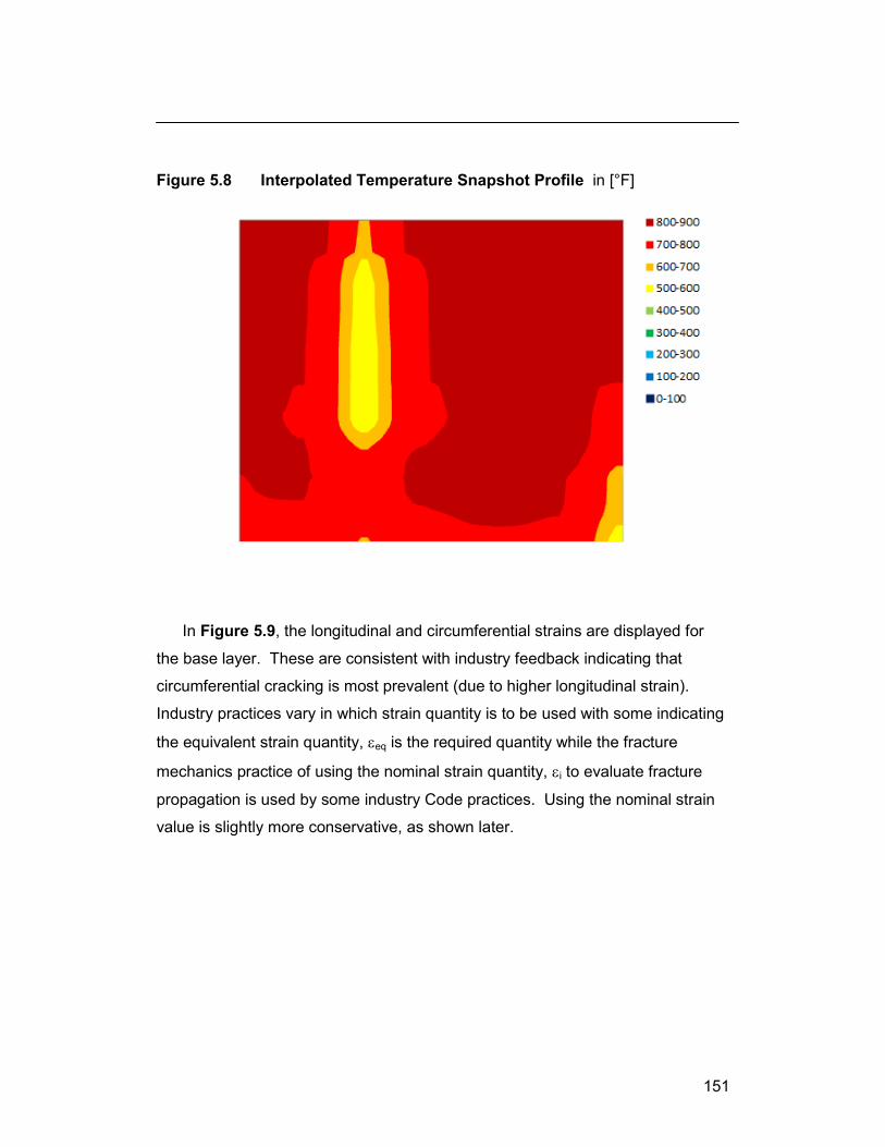
151

Figure 5.8 Interpolated Temperature Snapshot Profile in [°F]

In Figure 5.9, the longitudinal and circumferential strains are displayed for

the base layer. These are consistent with industry feedback indicating that

circumferential cracking is most prevalent (due to higher longitudinal strain).

Industry practices vary in which strain quantity is to be used with some indicating

the equivalent strain quantity, eq is the required quantity while the fracture

mechanics practice of using the nominal strain quantity, i to evaluate fracture

propagation is used by some industry Code practices. Using the nominal strain

value is slightly more conservative, as shown later.

152

Figure 5.9 Circumferential, Longitudinal Strain Snapshot Profiles in []

Notes to Figure 5.9

1. cylindrical coordinate system is used 2. Y ≡ circumferential / tangential direction; also “t” 3. Z ≡ longitudinal / axial direction 4. r ≡ radial direction 5. subscript “2” refers to base layer 6. CTE for the base and clad layers differ 7. strain profile for base layer, only shown for clarity

In this figure, the compressive longitudinal strains are located in the “hot” regions

immediately adjacent to the tensile longitudinal strain of 1,930 strain in the “cold

spot” evident in Figure 5.8. The circumferential strains (labelled as mech – Y2)

are much less and attributable to the reduced stiffness of the shell in the

circumferential direction.

z

t

r

153

Flexural Rigidity From bending theory of circular cylindrical shells, it is known

that the flexural rigidity of a cylinder is given by [57]

)1(12 2

3

tED (5.8)

The internal bending moments when radial deflections are imposed are

x

xx

DM

DM

(5.9)

where,

Mx ≡ the internal moment in axial direction associated with κx

Mθ ≡ internal moment in circumferential direction associated with κx

κx ≡ is the change of curvature in axial direction

υ ≡ Poisson’s ratio

The indicates that the internal bending moment in the circumferential direction

will always be less than the internal bending moment in the axial direction for the

shell of a cylinder when subjected to radial displacement.

154

In Figure 5.10, consecutive strain snapshots, for another sequence, are

plotted for a specific location to reveal that the strain response is positive

(tensile). The data in Figure 5.10 is presented for the portion of the total

operational cycle focused on the quench stage; prior to the quench stage, the

thermo-mechanical strain profile initiates at a value of zero (i.e., there is no

mechanical strain at ambient / reference temperature) and rises proportionally

with the increase in temperature, as operation proceeds, as profiled in Figure

3.3.

Figure 5.10 Strain Evolution in Clad and Base during Water Quench

Notes to Figure 5.10

1. Z, 1 ≡ nominal strain in axial direction, material 1 (clad)

Z, 2 ≡ nominal strain in axial direction, material 2 (base)

Y, 1 ≡ nominal strain in circumferential direction 1 (clad)

Y, 2 ≡ nominal strain in circumferential direction 2 (base) 2. Abscissa represents snapshot points during course of quench phase

The strain values, starting at the left edge of the plot, shown in Figure 5.10

correspond to the thermo-mechanical strain induced by the mismatch in

coefficient of expansion [CTE] between clad and base material layers and

calculable by closed form solution, as demonstrated.

155

Using equation (2.6), for the clad layer

c

bb

cc

chcb

cE

Et

Et

ETT 1

1

)()( 0

(5.10)

and, on substitution (using data from Figures 7.1, 7.2);

418,1

0.201

8.21118.01

)100900()2.72.9(

c

(5.11)

For the base layer;

b

bc

cb

bhcb

bE

Et

Et

ETT 1

1

)()( 0

(5.12)

and, on substitution;

156

0.20118.0

8.2111

)100900()2.72.9(

b

(5.13)

This demonstrates that the thermo-mechanical strain evolution prior to the start

of quench is governed by the CTE mismatch.

Repeating this for other operational cycles reveals that the individual

operational cycles are predominantly either positive (tensile) or negative

(compressive) during the thermal transient event occassioned by water

quenching.

156

Also to note, is that the strain response in the circumferential direction is

much less in both clad and base material layers; this aligns with the industry

observation that weld crack development is much less in the circumferential

direction for coke drums. This effort is completed for each data point for fifty two

(52) operational cycles to produce the strain exposure block histograms.

In Figure 5.11a-c, the maximum and minimum longitudinal strains occurring

at a single location in clad and base material layers, are plotted for the fifty two

(52) operational cycles that were reviewed.

Figure 5.11a Longitudinal Max / Min Strain, Clad in 52 Operational Cycles

157

Figure 5.11b Longitudinal Max / Min Strain, Base in 52 Operational Cycles

Figure 5.11b shows that that the evolution of a large tensile strain (cold spot)

during an operational cycle does not necessarily pair with a large compressive

strain (hot spot) during the same operational cycle; as well, the opposite

condition where a compressive strain (hot spot) precedes evolution of a tensile

strain (cold spot) is not evident. Hot and cold spots occur in random manner /

spectrum loading at any given location from operational cycle to cycle

158

Figure 5.11c Circumferential Max Min Strain, Clad in 52 Operational Cycles

Figure 5.11d Circumferential Max Min Strain, Base in 52 Operational Cycles

It is readily observed that the circumferential strains for clad and base

material layers, Figures 5.11c, d are much lower than the respective axial /

longitudinal strains given in Figures 5.11a, b falling well below the threshold

fatigue strain exposure of 3,000 (the conservative lower bound for fatigue

damage as established in Figure 2.13).

159

However, for the axial direction, it can be seen that the tensile profiles for the

clad and base track consistently; wherever large tensile strain excursions occur

for the base layer, the clad layer also exhibits a comparable excursion. For

compressive strains, the clad layer does not apparently track the strain profile of

the base layer; instead, only three small, compressive strain excursions are

noted which match the very large compressive strain loadings imposed on the

base layer. Thus, while the base layer experiences large tensile and

compressive strain exposures, the clad layer experiences essentially, only, a

tensile strain exposure. This is indicative of the “pre-load” effect of the large

tensile strain developed in the clad material layer which is due to the mismatch in

the coefficients of expansion between clad and base materials.

Industry practice, to date, has been to declare the difference between the

measured maximum / minimum strains, as measured on the base material

layers, during an operational cycle as the strain range. As shown by Figure

5.11b, these “strain range” values correspond to the strain exposure distributions

cited in the literature as previously presented in Figures 3.21 to 3.23.

Mistakenly, these values have been used to enter industry design fatigue life

limits.

The results of Figures 5.11a-b are re-ordered to assemble the correct strain

ranges to illustrate the impact and are presented as Figure 5.12a and Figure

5.12b for clad and base material layers, respectively.

160

Figure 5.12a Strain Range Assembly for Clad Layer, Axial Direction

Figure 5.12b Strain Range Assembly for Base Layer, Axial Direction

The appropriate strain ranges for clad and base materials are then appropriately

recast and presented in Figures 5.13a, b respectively.

161

Figure 5.13a Strain Range for Clad Layer, Axial Direction

Figure 5.13b Strain Range for Base Layer, Axial Direction

From these recast figures, it is readily observed that the base layer

experiences, in comparison to the clad layer, a larger apparent strain range

(5,375 to 4,750 ) and with similar number of exposures (7 to 7) over a

threshold value of 3,000 .

162

5.7 Mean Strain Effects

The clad layer experiences a reduced apparent strain range; but, the strain

exposure is mostly tensile resulting in a possible mean strain effect. The impact

of mean strain for clad and base can be estimated using equations (2.1) for no

mean strain and equation (4.13) to account for mean strain. For convenience,

these equations are repeated;

(5.14) and, to account for mean strain / stress;

(5.15) Hence, the effect of mean strain / stress can be computed and summarized in

Table 5.2.

Table 5.2 Cyclic Service Life with Specific Mean Strain Effects Cycle Clad Base

Count Nf ratio, Nf ratio,

R = -1 R ≠ -1 % R = -1 R ≠ -1 % 1 4,776 18,700 9,350 50 5,279 7,850 7,320 93 2 4,320 27,850 13,350 48 4,822 10,400 9,450 91 3 4,200 31,050 14,800 48 4,692 11,350 10,300 91 4 3,740 51,500 23,250 45 4,315 14,950 13,150 88 5 3,336 87,200 37,800 43 3,962 20,000 17,850 89 6 3,405 34,700 32,200 92 7 3,343 37,200 34,400 93

Notes 1. R = -1 defines fully reversed cycling; R ≠ -1 defines cycling with mean strain 2. Mean strain effects are determined by the modified Morrow equation (5.15) 3. ratio ≡ (Nf accounting for mean strain) / (Nf for fully reversed conditions)

cff

bf

fa NN

E 22 '

'

cff

bf

mfa NN

E

22 '

'

163

From Table 5.2, the service fatigue life counts for clad and base are

comparable for equivalent strain exposures; however, actual failure could be

expected to initiate slightly sooner and more often in the base layer since it

experiences a slightly larger strain range exposure profile, but that cracking

would present in either material.

This is evidenced by industry survey which indicated that “64% of surveys

indicated that cracks initiated from the ID while 71% indicated that cracks

initiated from the OD” [13]. The survey summarized that the occurrence of ID /

OD cracking was comparable. The survey also reported that 97% of survey

responses indicated cracks were primarily circumferential which agrees

conclusively with the thermo-mechanical strain data in Figures 5.11a-d.

The further evaluation of the clad material layer strain exposure would

proceed identically to the evaluation for the base layer and provides no further

insights into estimation of fatigue service life for the coke drum. The service life

fatigue assessment methodology, being general, can be explicitly applied to the

clad layer as specific details for a specific application would demand. In

development of this work, this effort is not warranted and redundant.

The data and calculations above indicate that there is an initial biaxial strain

induced in the clad of approximately 1,500 during the initial portion of the coke

drum operational cycle which starts at steam test / vapor heat to completion of oil

fill (Figure 3.3, 4.8). The data (Figure 5.11a) shows that the induced strain in

the clad increases during formation of a “cold spot” but during formation of a “hot

spot”, the clad layer seldom reaches a negative strain state. Hence, the effect of

the CTE mismatch is to cause the clad layer to “pre-load” and limit the majority of

strain range exposures in the clad material layer to less than the low cycle

threshold damage level (3,000 ). This suggests the clad layer also serves a

useful mechanical role, in addition to serving as a corrosion protection liner.

164

The strain ranges assembled in Figures 5.12a, b and Figures 5.13a, b

conform to the cycle counting methods recognized in industry practices and the

Code, specifically.

While many schemes are available for spectrum loading [15, 29], ASME VIII

Division 2 [7] explicitly references two methods taken from [58]

rainflow method

max – min method (peak or level crossing counting)

Using the later due to its computational convenience, clarity and conservatism,

range cycles were determined from pairing the maximum strain reversal with the

minimum strain reversal, then continuing to the next peak – valley pair and so on

to completion for the representative duty block. The duty block is the collection

of strain reversals occurring during subsequent operational cycles which fairly

represents the strain exposure for a location.

165

Commentary on Thermo-mechanical Strain Range The strain quantities

displayed in the forgoing are those due to thermo-mechanical loading, only.

Other mechanical loadings have been disregarded and based on their impact

upon the net strain range exposure.

In Figure 2.9, it was demonstrated that the correct strain range to consider

for cyclic loading was the Code compliant strain range and cycle count. The

effect of considering the operating pressure load of 35 psig is to impart a biaxial

stress field resulting in a triaxial strain field. The nominal strains, calculated from

strength of materials consideration vary and are a maximum for the hoop

(circumferential) direction of

(5.16)

The mechanical strain contribution from pressure and other mechanical loadings,

in this instance, have been disregarded for two primary reasons;

1. the pressure strain of 172.3 is small 2. the sustained loads are constant over the operational cycle and do not

substantively impact the fatigue range

3.1720625,23.0250,59.25

1

1

250,51

15035

rlhh

h

vE

and

psit

pr

166

In Figure 5.14, the mechanical strain, due to pressure loading, is added to

the mechanical strain determination from thermal loading, i.e., the thermo-

mechanical strain. It is seen, by comparison to Figure 2.9 that the net effect on

the strain range is zero (0). An inconsequential impact from mean strain effects

may be noted., but is small in this instance.

Figure 5.14 Pressure Strain & Thermo – mechanical Strain Range

Simplified Strain Range Component Determination Industry practices

consider use of either the equivalent or structural stress methodology to calculate

the strain range [7, 8]. In Table 5.3, a simplified structural stress component

approach is applied. The mechanical strain components are retrieved for the

maximum and minimum strain values presented for the base material layer in

Figure 5.12b corresponding to operational cycle # 4 and cycle # 3, respectively

in Figure 5.11a. The strain range is calculated on a strain component-by-

component basis to determine the von Mises / equivalent mechanical strain.

167

The top and bottom surfaces were not treated explicitly since both values are

nearly identical to the membrane component, typically < 5% difference. It is also

apparent that the equivalent strain value differs from the structural stress value

by about 15%, the equivalent strain being smaller and, hence, less conservative.

Industry practices specify using the equivalent strain / stress (von Mises strain /

stress) in design for strength [7, 8]. However, designers are not prevented from

using more conservative criteria.

The computational burden of calculating the equivalent strain is much greater

and is not justified given the purpose of estimating a service life where other

uncertainties are greater (i.e., variability in fatigue life, refer to Figures 2.6, 2.13).

The more conservative approach of using the difference in strain components is

reasonable in this instance.

168

Table 5.3 Strain Range Determination, Mechanical Strain Components in strain component von Mises

Layer Cycle Surface X Y Z vM

Clad # 4 Top - 1,692 293 3,654 Bot - 1,743 383 3,683 Mem -1,717 338 3,669 # 3 Top - 163 1,381 - 1,000 Bot - 149 1,338 - 989 Mem - 156 1,359 - 995

X Y Z

Top - 1,528 - 1,088 4,654 3,983 Bot - 1,593 - 955 4,673 3,982 Mem - 1,561 - 1,021 4,663 3,982

Base # 4 Top - 816 - 974 2,879 Bot - 1,252 - 219 3,141 Mem - 1,034 - 597 3,010 # 3 Top 637 679 - 2,164 Bot 757 307 - 2,074 Mem 697 493 - 2,119

X Y Z

Top -1,453 - 1,653 5,043 4,399 Bot - 2,009 - 526 5,215 4,406 Mem - 1,731 - 1,090 5,129 4,375

Damage Exposure The data shows that a small portion of events, 7 of 52

instances (< 15%) exceeds a strain range of 3,000 strain; in Figure 2.3 it was

shown that strain ranges below 3,000 strain have a very long cyclic life,

exceeding 100,000 cycles or nominally, 270 years of coke drum operation.

Therefore, only those strain range exposures exceeding 3,000 strain are

considered to be damaging.

169

This exposure distribution is exhibited in Figure 5.15. This presents the

thermo-mechanical strain distribution for a single, base material data point for 52

cycles.

Figure 5.15 Strain Distribution, Single Location for 52 Operational Cycles

The strain exposure distriubution for the 20 interior data points, in the base

material, for the 52 operational exposures is presented in Figure 5.16. The data

is consistent with the strain distribution for the single data point in that the

damaging strain exposures are less than 15% of the total strain exposures

caused by thermo-mechanical fatigue.

170

Figure 5.16 Strain Distribution, 20 Locations for 52 Operational Cycles

171

5.7 Strain Exposure Profile and Cyclic Life Criteria

To determine the cyclic life of an as – constructed coke drum, the

representative thermo-mechanical strain loading profile is applied to the strain

fatigue life curve for the material of construction.

The categorical thermo-mechanical loading profile for the data points of

Figure 5.16 is expanded and recast as Figure 5.17.

Figure 5.17 Strain Exposure – 52 Operational Cycles

This data can be re-arranged to establish bounding curves in order to

establish the 1% and 99% confidence limits for the exposure profile shown in

Figure 5.18.

172

Figure 5.18 Strain Range Exposures – 52 Cycles

The data from Figure 5.18 is use to enter Figure 5.19 which presents the

combined strain – cyclic service life curve for the commonly used materials of

construction for coke drums compiled from the data presented in § 2.

Figure 5.19 99% Confidence Level – Cyclic Service Life

173

To enter Figure 5.19, the upper bound curve of Figure 5.18 is used to enter

the the bounding curve of Figure 5.19; the anticipated, unconditioned fatigue life

would be 23,255 operational cycles [96 years at the 99% confidence limit]. In

addition, the lower bound curve of Figure 5.18 is used to enter the same

bounding curve Figure 5.19 for which the anticipated upper bound,

unconditioned service fatigue life is calculated as 111,690 operational cycles

[460 years at the 1% confidence limit]. These yearly values assume a nominal

operational duty cycle of 24 hours. The Palmgren – Miner damage accumulation

model is used in conformance to industry practice and is detailed in the next

chapter. The fatigue service life is reported as an “unconditioned” life estimate

since it does not account for localized effects from weldments (which contain

Code acceptable internal defects, residual stresses) and shell distortions.

The literature suggests coke drum life is from twenty to fifty years. Figure

5.20 is taken from reference [13] and indicates more than 100 cracks for a drum

with less than 3,000 operational cycles [ 8 years ] and several drums

experiencing apparent accelerated cracking after reaching 6,000 operational

cycles [16 years].

174

Figure 5.20 Total Number of Cracks vs Total Number of Cycles

In Figure 5.21, a single drum is shown with approximately 20,000 cycles / 54

years with a gap in data showing that the bulk of drums, in the survey consisting

of 145 drums, have exposures of less than 10,000 cycles / 27 years. Chevron

Corporation indicates a coke drum was replaced at the El Segundo, California

refinery which had a service life of forty six years [59]. Actual life is indicative of

the complication of shell distortions, otherwise described as shell bulging.

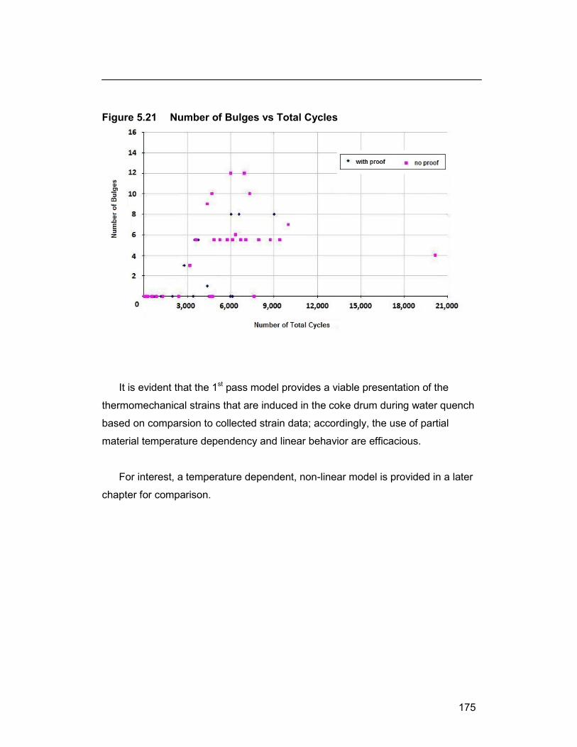
175

Figure 5.21 Number of Bulges vs Total Cycles

It is evident that the 1st pass model provides a viable presentation of the

thermomechanical strains that are induced in the coke drum during water quench

based on comparsion to collected strain data; accordingly, the use of partial

material temperature dependency and linear behavior are efficacious.

For interest, a temperature dependent, non-linear model is provided in a later

chapter for comparison.

176

CHAPTER 6 CYCLIC LIFE DETERMINATION FOR A COKE DRUM

When a new coke drum is exposed to thermo-mechanical loading, damage is

eventually incurred in the form of shell bluging and cracking. Cracking may occur

at shell welds, in unwelded portions of the shell plate or at shell bulges. The

mechanism of shell bulging is not definitively explicated in the literature with only

some competing notions stated. These include

coke crushing

weld strength mismatch

hot & cold region formation

This thesis examines cracking at both undistorted and distorted shell areas;

this work does not address the specific causes of bulge formation but, rather, the

consequences of these general shell distortions. Although all three possible

causes can contribute to shell distortion damage, the most plausible leading

cause is hot and cold shell region formation.

Shell bulging is classified as a general shell distortion in several industry

trade publications. Two authors have attempted to address shell bulging by

indirect assessment methodologies which will also be described.

6.1 Industry Practice Code and Standards

ASME / API Documents

Standard industry documents ASME VIII Division 1 and Division 2 and dual

marked API 579 –1 / ASME FFS –1 deal with shell dimensional tolerances.

Since ASME VIII Division 1 and Division 2 are intended for new construction,

discussion of deviations in shell dimension are limited to shell out – of –

roundness. The acceptable tolerance on shell out – of – roundness, Dmax – Dmin

is limited to 1% of D per paragraph UG – 80(a) of Division 1 and Division 2

paragraph AF – 130.1. Both of these pressure vessel construction Codes do not

address peaking of welds. Peaking is an industry idiom referring to angular

misalignment of longitudinal and circumferential weld joints.

177

However, ASME VIII Division 2 does require that the dimensions characterizing

the peaking distortion are to be measured and included in the fatigue analysis of

the vessel, if a general fatigue analysis has been deemed necessary.

An industry document not usually referenced for pressure vessel work is API

Standard 650 applying to welded steel oil storage tanks [60]. Oil storage tanks

can be very large, exceeding 250 feet [76 m] in diameter and fabricated from

1inch to 2 inch [25.4 mm to 50.8mm] thick steel plate. Due to their large

diameter to thickness ratio, D / t, the standard provides for an explicit rules –

based limit on shell peaking. Peaking is not to exceed ½ inch [13 mm] in a 36

inch [900 mm] sweep board in both longitudinal and circumferential directions.

This rule sets a lower limit for assessment of a coke drum.

ASME VIII Division 2 provides for a fatigue analysis on the basis of a simplified

elastic – plastic analysis which uses a penalty factor technique. Analysis using

elastic – plastic analysis is recognized but not mandatory.

API 579 – 1 / ASME FFS –1 Level 2 Evaluation

To quantify the impact of peaking in longitudinal and circumferential welded joints

or plate, API 579 – 1 / ASME FFS –1 provides a closed form approach,

presented as a Level 2 analysis approach. A finite element study would be

considered as a Level 3 evaluation.

The Level 2 assessment methods are completed by closed form solutions.

The method of API 579 – 1 / ASME FFS –1 determines a secondary stress load

due to axial and angular misalignments. Since modern coke drum construction

methods use single thickness shell plates, axial misalignment is not a primary

consideration. However, the effect of bulges and general shell distortion is to

impose angular and bulge misalignments.

178

The API / ASME practice standard calculates a ratio of induced bending stress to

the applied membrane stress in a component that results from pressure. A

second ratio of induced bending stress to the applied membrane stress from

supplemental loads is under development.

Bulge Intensity Factor (BIF™) [27]

Samman describes an intuitive technique for assessing the severity of shell

misalignments using the notion of bulge intensity factor [BIF™].

The authors indicate that the motivation for the technique arose from the

apparent lack of correlation between stress profiles generated from finite element

analyses and shell cracking histories. They attribute the lack of correlation to

inability to assess stresses from thermal transients during the fill cycle and by

shell-coke interaction during the quench cycle. The authors cite the work of

Farraro & Boswell – 1996 [21] and, Boswell – 1997, Boswell & Farraro – 1998

[61].

Significantly, the thermo-mechanical loading during the quench cycle is

referenced as a further complication together with shell bulging rendering

analysis far too complex. Therefore, a simplified methodology is needed. The

BIF™ parameter is based on pattern recognition techniques and, for coke drums

is utilized to discern geometric features associated with cracking failure. Thus,

the technique is heuristic and dependent on a sufficient database of geometries

and associated shell cracking failures.

Accordingly, there are no publicly available calculation protocols and reliance is

based on a ranking scheme dependent on a proprietary algorithm.

179

Plastic Strain Index [PSI™] [27]

Samman et al. state the shortcomings of the API 579 –1 / ASME FFS –1 practice

standard in assessing coke drum shell bulges using the Level 3 approach, i.e.,

numerical analysis, and the inaccuracy of the Level 2 assessment techniques

therein.

The reasons for these shortcomings are attributed to the complex and random

nature of thermo-mechanical loads [26].

The authors suggest that a numerical analysis using elastic – plastic methods

and using the strain criteria of API 579 –1 / ASME FFS –1 would provide a

determination of equipment suitability for continued operation. The numerical

analysis is based on pressure loading only. To facilitate communication of these

results, the authors ranked the results of the strain analysis against the limit

strain criteria defined in the practice document.

The practice standard defines the limit strain as a function of several factors;

applied stress

material yield strength

material tensile strength

material reduction of area

a multi-axial material strain limit value, sl = 2.2 for ferritic steels

The basis of the strain limit according to the practice standard is monotonic

loading.

The index rankings are linear; ranking of severity grade, crack likelihood and

monitoring frequency being qualitative and apparently arbitrary. Table 6.1 is

provided for illustration of the method.

180

Table 6.1 Plastic Strain Index Severity Grades per Samman [27]

% strain limit

Severity Grade

Likelihood of Bulged-Induced Crack

Monitoring Frequency

80 to 100 Failure Likely ½ – 1 year 60 to 80 Danger Probable 1 year

40 to 60 Concern Possible 1 – 2 years

0 to 40 Design Unlikely 2 – 3 years

Bulge Severity Factor

Araque et al. [37] define the Bulge Severity Factor [BSF] using the ratio of

longitudinal stress for the damaged geometry to the longitudinal stress for the

undamaged geometry of a coke drum considering only the primary pressure and

weight loads according to

undamaged

damagedBSF

(6.1)

The BSF, therefore, is a stress concentration factor. The investigators also use a

temperature interpolation scheme to develop a temperature distribution for

intermediate data points. The heuristic scheme uses convective heat transfer

analysis to force calculated temperatures to match temperatures at known data

points. The investigators state that a linear interpolation scheme was required to

reduce the time step for achieving convergence in stress analysis. The

investigators reported significant stress oscillations in the analytical model which

forced use of a 0.25 second time step. Mesh sizing was reduced to 18 mm x 18

mm [0.7 inch x 0.7 inch] to achieve convergence.

181

Analysis was made using the pseudo-elastic stress basis. BSF stress

concentrations approaching 8 were determined. This was combined with use of

a fatigue strength reduction factor of 2 to enter the traditional stress – fatigue life

curve of ASME VIII Division 3 [62]. This Code is intended to be used for high

pressure vessels where pressure exceeds 10,000 psi [70 MPa] although lower

pressure applications in the order of 1,000 to 3000 psi [6.9 to 20.7 MPa] are

treated using the Division 3 methods. The authors do not indicate why this Code

was used in preference to the expected industry practice documents.

6.2 Deterministic Approaches to Coke Drum Life Evaluation

Coke drum fatigue cracking failure has been problematic for the industry

since the earliest installations made in the 1930’s.

Focused efforts in defining the problem and identifying solutions began in the

1950’s with publication of the survey performed by Weil and Rapasky who

worked for an industry engineering contractor, M W Kellogg [3]. Later work was

undertaken by industry trade groups such as the API and the MPC.

The difficulties for the investigators was a lack of numerical data and

technology, specifically

finite element analysis software

coke drum shell temperature data

coke drum strain data

materials of construction data

calculation methodology

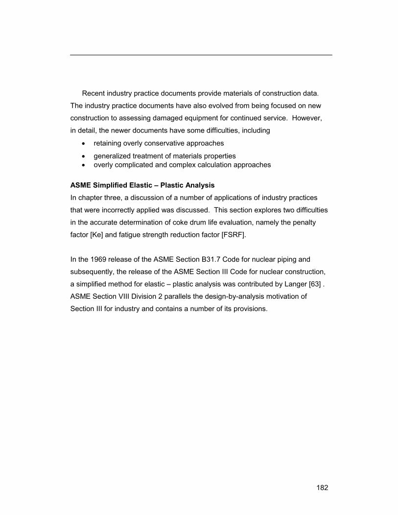
182

Recent industry practice documents provide materials of construction data.

The industry practice documents have also evolved from being focused on new

construction to assessing damaged equipment for continued service. However,

in detail, the newer documents have some difficulties, including

retaining overly conservative approaches

generalized treatment of materials properties

overly complicated and complex calculation approaches

ASME Simplified Elastic – Plastic Analysis

In chapter three, a discussion of a number of applications of industry practices

that were incorrectly applied was discussed. This section explores two difficulties

in the accurate determination of coke drum life evaluation, namely the penalty

factor [Ke] and fatigue strength reduction factor [FSRF].

In the 1969 release of the ASME Section B31.7 Code for nuclear piping and

subsequently, the release of the ASME Section III Code for nuclear construction,

a simplified method for elastic – plastic analysis was contributed by Langer [63] .

ASME Section VIII Division 2 parallels the design-by-analysis motivation of

Section III for industry and contains a number of its provisions.

183

ASME VIII Division 2 FSRF and Penalty Factor Ke

The Code provides for a simplified elastic – plastic analysis using a penalty factor

approach whenever the local stress exceeds two times the specified minimum

yield strength of the material.

Ke = 1.0 for Sn ≤ SPS (6.2)

= 1.0 + (1 − n) · (Sn / SPS − 1) for SPS < Sn < m·SPS (6.3)

n(m − 1)

= 1/n for Sn ≥ m·SPS (6.4) Sn = range of primary plus secondary stress intensity SPS = allowable limit on the primary plus secondary stress range;

SPS is the larger of 3 times the average of S at lowest and highest temperature during the operational cycle or 2 times the average of SMYS at the lowest and highest during the operational cycle

S = allowable stress based for the material of construction

n, m define material constants, with

n = 0.2 for low alloy steels such as C – ½ Mo, Cr – Mo and C – Mn – Mo

steels m = 2.0 for low alloy steels

Figure 6.1 illustrates the scheme used by ASME for the simplified approach.

The intent of the procedure is to use the elastic numerical analysis and condition

it for stress and strain concentration without the necessity of conducting an

explicit elastic-plastic analysis prior to entering the fatigue life curves [7].

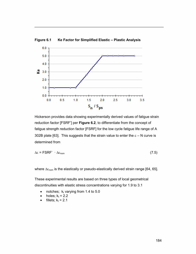
184

Figure 6.1 Ke Factor for Simplified Elastic – Plastic Analysis

Hickerson provides data showing experimentally derived values of fatigue strain

reduction factor [FSRF’] per Figure 6.2, to differentiate from the concept of

fatigue strength reduction factor [FSRF] for the low cycle fatigue life range of A

302B plate [63]. This suggests that the strain value to enter the – N curve is

determined from

= FSRF’ · nom (7.5)

where nom is the elastically or pseudo-elastically derived strain range [64, 65].

These experimental results are based on three types of local geometrical

discontinuities with elastic stress concentrations varying for 1.9 to 3.1

notches; kt varying from 1.4 to 5.0

holes; kt = 2.2

fillets; kt = 2.1

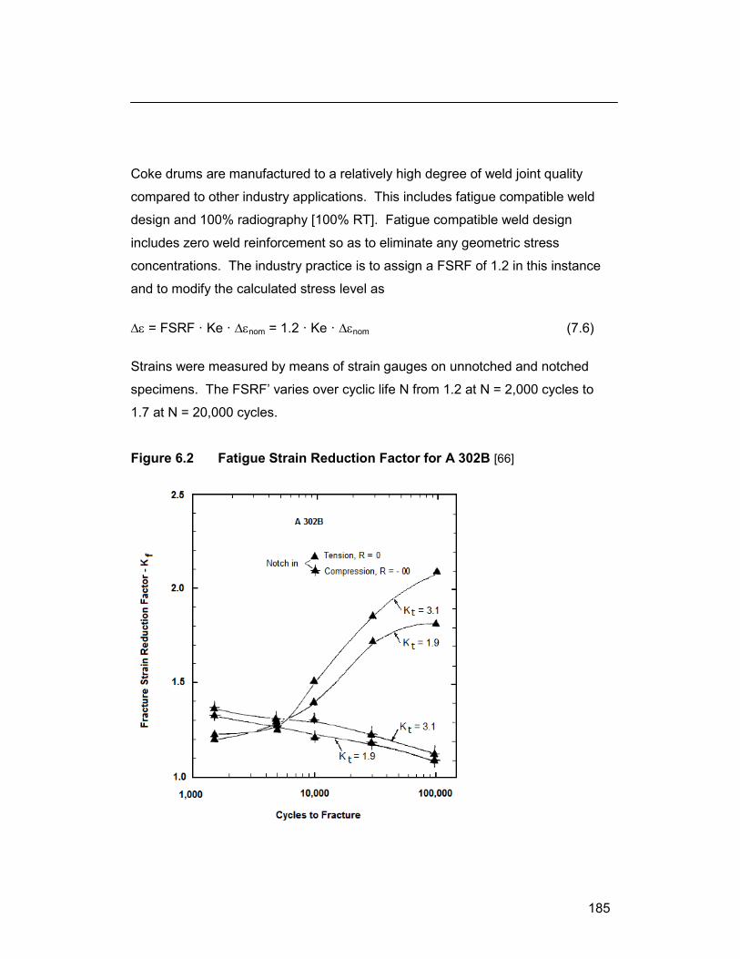
185

Coke drums are manufactured to a relatively high degree of weld joint quality

compared to other industry applications. This includes fatigue compatible weld

design and 100% radiography [100% RT]. Fatigue compatible weld design

includes zero weld reinforcement so as to eliminate any geometric stress

concentrations. The industry practice is to assign a FSRF of 1.2 in this instance

and to modify the calculated stress level as

= FSRF · Ke · nom = 1.2 · Ke · nom (7.6)

Strains were measured by means of strain gauges on unnotched and notched

specimens. The FSRF’ varies over cyclic life N from 1.2 at N = 2,000 cycles to

1.7 at N = 20,000 cycles.

Figure 6.2 Fatigue Strain Reduction Factor for A 302B [66]

186

The same trend is displayed in Figure 6.3, also provided by Hickerson. The data

of Figures 6.2 and 6.3 is in contradiction to the direction of current industry

practices provided in the Code [7]. Whereas the fatigue strength reduction factor

is given as a constant depending on weld fabrication quality and independent of

stress concentration, experimental data suggests that the fatigue strength

reduction factor is

a function of geometric stress concentration

a function of stress / strain level

a function of stress / strain direction (compressive / tensile)

accounts for non-linearity implicitly

Figure 6.3 Fatigue Strain Reduction Factor [66]

Chen’s data is in agreement with the work of Hickerson for R = 0 and shows a

positive relationship of FSRF to cyclic count, i.e., FSRF increases as strain

decreases [66].

187

Chen studied two types of notches in fully reversed loading (R= -1), one

associated with the weld material and the second associated with the weld heat

affected zone. The FSRF, studied by Chen, associated with the weld material

corresponds with the Hickerson studies. The FSRF, studied by Chen, associated

with the HAZ shows increasing strength reduction with cyclic life (reduced strain).

Figure 6.4 Fatigue Strength Reduction Factor [35]

The source data for Chen’s results is derived from the experimental data

presented in Figure 6.5. It can be seen that the fatigue life diverges for the three

material types as cyclic strain exposure level decreases, i.e. cyclic life, N

increases, consistent with the tensile testing regime of Figures 6.2 and 6.3.

188

Figure 6.5 Strain – Life Data Establish FSRF in [35]

In contrast, testing by Ramos showed, using Figure 6.6, a converging fatigue

life for the two material areas as cyclic strain exposure level decreases, i.e. cyclic

life N increases, consistent with the compressive testing regime (R = – ∞) of

Figures 6.2 and 6.3.

189

Figure 6.6 Strain – Life Data from Ramos to Establish FSRF [19]

The apparent FSRF suggested in Figure 6.6, presented in Figure 6.7, is

seen increasing to a limit value (strain increasing) of 4.0 and is consistent with

the practice of some industry practitioners to use an FSRF of 2.0 for complete

joint penetration (buttwelds) in fatigue calculations.

190

Figure 6.7 Fatigue Strength Reduction Factor [19]

Papers Slagis reviews that the first appearance of “simplified elastic-plastic discontinuity

analysis” occurred with publication of rules for nuclear piping in 1969 [67]. These

were then incorporated into the ASME III rules for construction of nuclear vessels

in 1971 and piping rules were incorporated into the Section III rules. The Code

allowed certain primary-plus-secondary stresses to exceed the stress limit of

3·Sm if a penalty was taken on the fatigue analysis. This penalty was designated

as the penalty factor, Ke and was designed to vary with the stress level and was

a function of material property. For low alloy steel, Ke could be as much as 5.0.

Slagis advises that additional testing showed that the penalty factor was too large

and other codes have proposed lower values [63].

191

The meaning of Ke was given by Langer [68] Strain concentration can occur in any structural member with stress gradients as soon as the

loading exceeds the point at which the highest-stressed region becomes plastic. If the plastic zone

is highly localized, the surrounding elastic material controls the strain in the plastic material and

no strain concentration occurs. When the plastic zone is large enough to become a significant

factor in the stress distribution, however, the strains in the plastic zone become larger than those

which would be calculated by the theory of elasticity and strain concentration must be considered.

Langer calculated plastic strain concentration factors on a tapered flat bar in

tension and a cantilevered beam in bending to establish that the limiting value of

Ke = 1 / n. For low alloy steels, n = 0.2.

Testing by Gerber using cylindrical specimens with two types of local

discontinuities, groove and shoulder with an elastic stress concentration of 2.0

against a smooth specimen established that Ke was about 2.2 for Sn / 2•SMYS =

2 for carbon steel [63, 69].

Krempl defined the fatigue strength reduction factor as [64]

bar unnotched of stress nominal

bar notched of stress nominalk f

S

S n and, (7.7)

found for 2¼ Cr – 1Mo material that kf approached ~ 1.0 in the plastic region. Slagis provides data from Japanese research by Iida indicating that a Ke value

approaching 2.0 should be used for kt values of 1.85 to 2.26 over a temperature

range from room temperature to 575 °F [300 °C] over a ratio of / 2*Y from 0.5

to 3.25 as shown in Figure 6.8 [70]. The experimentally derived value was found

to be slightly higher than the calculation methodology of Neuber.

192

Figure 6.8 Ke Data – Slagis [70]

Discussion

The data and indications suggest the ASME Ke values are overly simplistic, very

conservative and not appropriate for determining service fatigue life. This

approach needs, however, to be retained for determination of the design fatigue

life in order to comply with current Code design requirements.

The FSRF approach suggested by Slagis, Iida, Krempl and Hickerson is a more

vigorous method and should be used for the determination of service fatigue life.

A complicating attribute, as shown by the testing of Hickerson and Chen is that

the FSRF is dependent on strain loading direction, i.e. tensile or compressive;

fully reversed loading appears to track tensile strain cycling.

FSRF values varying from 1.2 to 2.2, as a function of strain level is appropriate

for the range of strain exposure experienced by a coke drum. The work of Chen

indicates that some caution is required in that the FSRF values associated with

failure of the HAZ can approach 4.0.

193

To progress a more robust approach, in view of the difficulty in assigning an

appropriate FSRF, is to consider using a lower bound material fatigue life curve,

- N that accounts for the scatter in welded materials. Both Ramos and Chen

have studied this in detail and their findings are provided in Figure 6.9.

Figure 6.9 Lower Bound Fatigue Life Curve – Welds, HAZ

In Figure 6.9, the lower bound curve (gray line) from Figure 5.19 is included

to show that the fatigue life of weld and HAZ zones is captured by the variability

in testing such that the lower bound curve established by the testing of base

materials may be used to establish coke drum service fatigue life without

recourse to the Code penalty approach.

While strain concentrations occur for a given material, they may be

pragmatically addressed by use of the proposed bounding curve. Where

warranted, specific service fatigue life data may be established.

194

6.3 Calculation of Strain Based Service Fatigue Life for a Coke Drum

The calculation of strain-based fatigue service life for a coke drum is

determinable using a phenomenological approach since;

– N, strain to low cycle fatigue life mechanical properties have been established for the main coke drum materials of construction, Figure 5.19

thermo-mechanical loading of the shell is probabilistic, see Figure 5.18

a simplified elastic – plastic analysis is practical and accurate without using the fatigue strength reduction factor, FSRF

the fatigue penalty factor, Ke as prescribed in the Code is overly conservative, and though more accurately established by Krempl and Hickerson, is not required for service life assessment

the damage to coke drum shells may be bound between two types of damage; angular misalignment and bulge misalignment

Service Fatigue Life of a Newly Constructed Coke Drum

The preceding sections have demonstrated that using a lower bound fatigue life

curve will provide the requisite accuracy in determination of a service fatigue life.

The life value is based on use of the damage accumulation expression wherein

0.11

k

km

k N

nD applies over the fatigue life. (6.8)

The efficacy of this expression is based on its inclusion in several pressure

vessel construction Codes and is not addressed in this work. The expression is

known as the Palmgren – Miner rule. Research data indicates the damage

criteria, D varies between 0.4 and 1.4 but that for reversed loading, a value of

1.0 is considered adequate [15, 33].

Strain exposures are defined in Figure 5.18 by taking the intersection of the

upper bound line for each of the 52 exposures as the 99% confidence level for

strain range loading, .

195

For each nk thus established, the corresponding Nk value is established from

Figure 5.19 by intercepting the strain exposure value with the lower bound curve

representing the 99% confidence level for cyclic life, N.

To exemplify the preceding;

enter Figure 5.18 at n1 = 1/52 (0.0192), intercept = 5,711

enter Figure 5.19 at = 5,711 , intercept N1 = 2,675 cycles

calculate n1 / N1 = 19.2 / 2,675 per 1,000 cycles

for < 3,500 , sum the remaining nk , set Nk = 100,000 cycles

complete nk / Nk = for all 52 exposures

sum the nk / Nk , this is the damage fraction for 1,000 cycles

calculate 1,000 / nk / Nk to obtain the number of cycles corresponding to D

= 1.0; designate as Ntotal

calculate service life, Nyears at the 99% confidence level as Ntotal / 365 assuming 1 operational cycle for each 24 hour period.

The calculated life, Nyears thus is 72 years at the 99% confidence level.

The 50% confidence interval is similarly calculated as 151 years for comparison.

Using the methodology established above, the service fatigue life of a newly constructed coke drum can be determined to be between 72 and 151 years, assuming one operational cycle every twenty four hours. This service life is limited by the quality of the undeformed shell welds.

Service Fatigue Life of a Damaged Coke Drum

Coke drums deteriorate in service from development of shell distortions. These

distortions were exhibited in Figure 5.1. All drums experience damage soon

after entering service; hence, a more informative and valued service life estimate

is given based on the actual physical condition of the drum.

There were no detailed damage profiles available in the literature; but some large

scale data was retrieved. Figure 6.10 shows a shell contour plot for a coke

drum; the maximum shell radial deviation is ± 2 inches [50.8 mm].

196

Figure 6.10 Drum Bulge Profile – Radial =2” [50.8 mm]

In Figure 6.11, the shell radial deviation is ± 4 inches [101.6 mm]. In both

drums, an accurate local profile is not available and is not provided in practice.

However, in order to bound the damage, two types of local damage profiles

can be considered;

an angular axial misalignment

a rounded axial misalignment

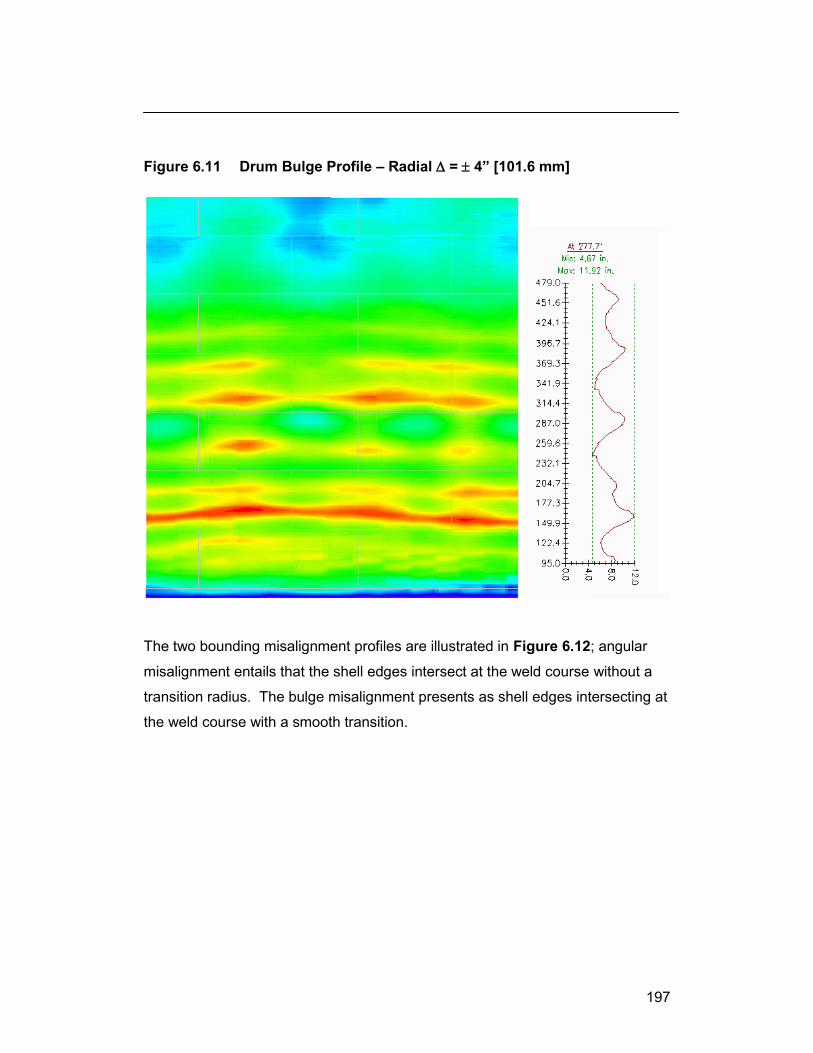
197

Figure 6.11 Drum Bulge Profile – Radial = 4” [101.6 mm]

The two bounding misalignment profiles are illustrated in Figure 6.12; angular

misalignment entails that the shell edges intersect at the weld course without a

transition radius. The bulge misalignment presents as shell edges intersecting at

the weld course with a smooth transition.

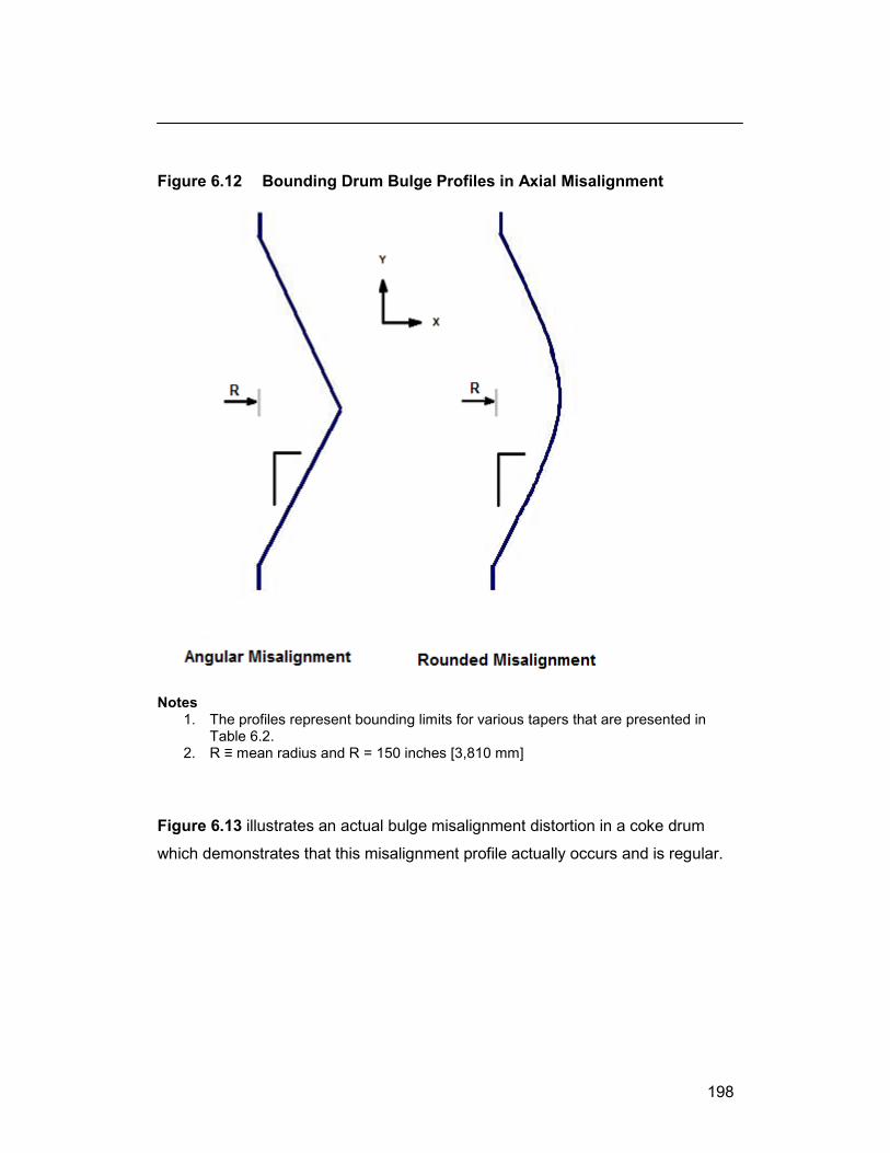
198

Figure 6.12 Bounding Drum Bulge Profiles in Axial Misalignment

Notes

1. The profiles represent bounding limits for various tapers that are presented in Table 6.2.

2. R ≡ mean radius and R = 150 inches [3,810 mm]

Figure 6.13 illustrates an actual bulge misalignment distortion in a coke drum

which demonstrates that this misalignment profile actually occurs and is regular.

199

Figure 6.13 Photograph of a Drum Bulge

To calculate the impact of shell distortion on service life, the previous procedural

scheme is modified to account for two considerations

the stress / strain concentration, kt caused by the alignment profile

the increased strain value with which the – N service life curve is entered

The stress / strain concentration factor is calculated using numerical methods

(i.e., FEA) for the several geometries presented by Figure 6.10, Figure 6.11

and within the constraints of Figure 6.14.

200

Figure 6.14 Bulge Growth in Damaged Drums [13]

Determination of kt Factors for Damaged Drums

The stress / strain concentration factors for a damaged drum can be determined

for the bounding profiles given in Figure 6.12. A complication is to recognize

that the stress / strain fields for pressure and thermal loading are different.

Whereas, pressure loading in a cyclinder creates a bi-axial, 2:1 hoop to axial

stress field, thermal loading presents a 1:1 stress field.

For specific industry application to a damaged drum, the dimensional data from a

laser scan will be used in construction of the shell numerical model. Hence,

strain results will inherently reflect stress / strain concentration effects caused by

dimensional distortions. Where detailed laser scans are not available, estimates

of drum shell distortions may be made from visual approximation.

To illustrate the impact on stress / strain results, the differences can be reviewed

for a sample defect under pressure and temperature loading.

201

In Figure 6.15, a quarter symmetry flat plate with hole is modeled; pressure and

temperature loading are applied under boundary conditions appropriate for the

loading.

Figure 6.15 ¼ Symmetry FEA Model for SCF Determination

Notes to Figure 6.1x

1. Flat panel, 1” [25.4 mm] thickness; SHELL4 element with 6 degrees of freedom 2. No out of plane displacement;

UZ = 0 under all conditions AR = at all edges

3. UX = 0 at left edge, for 1D pressure loading in X direction UX, UY = 0 at left, bottom edge for pressure loading in X, Y directions

4. UX = 0 at left, right edges, for 1D temperature loading UX, UY = 0 at all four straight edges 2D temperature loading

5. Pressure loading at free edges varied to suit loading ration regime; base pressure load of 5,250 psi applied, corresponding to hoop stress in coke drum

X

Y

202

The results are presented in Table 6.2 for pressure and temperature loading

cases. The data demonstrates that for temperature loading, under 2D restraint,

the SCF developed at the discontinuity is identical to a pressure loading using a

1:1 biaxial stress field. The 2D restraint field induces a 1:1 biaxial stress field in

the plate.

The SCF for a 2:1 pressure loading is 2.6 for the model (2.5 theoretical) and is

greater than the 2D restraint temperature loading case. Hence, the pressure

load is more conservative and can be used to estimate the effect of

discontinuities encountered under temperature loading of the damage models.

The primary purpose of this effort is to illustrate that thermomechanical loading

results in a smaller SCF value compared to pressure loading for the hole-in-plate

model and similar results are expected for the SCF for a bulged shell.

Table 6.2 Results for Pressure / Temperature Loading Cases

Theoretical Numerical

Value SCF Value SCF

[psi] [psi] % Pressure

1:0 15,750 3.0 16,602 3.2 6.7 1:1 10,500 2.0 10,945 2.1 5.0 2:1 13,125 2.5 13,638 2.6 4.0

Temperature (-100 F)

1D restraint 66,045 3.0 64,203 2.90 -3.3 2D restraint 44,030 2.0 61,270 1.98 -1.0

203

The SCF values for various damage conditions can be estimated from finite

element method models from the damage profiles presented in Figure 6.12. A

particularized model is presented as a rounded bulge in Figure 6.16.

Figure 6.16 Rounded Bulge in Axial Misalignment, FEA Model

204

Notes to Figure 6.16 1. The element used for the model is the SHELL4L 4-node multi-layer quadrilateral

shell element, 8,640 elements used; elements have

membrane and bending capabilities for the analysis of three-dimensional structural and thermal models

up to 50 layers can be used; 2 layers are used for this analysis

six degrees of freedom (3 translations and 3 rotations) are considered per node

each layer can be associated with different isotropic or orthotropic material properties; isotropic material behaviour is used for the model

2. UZ, UR, UT ≡ translational displacement; in the cylindrical coordinate system RZ, RR, RT ≡ rotational displacement; in the cylindrical coordinate system

3. The top edge of the model is coupled / constrained to preserve plane-remains-plane boundary condition; this ensures no local part of the model can displace relative to other elements on the boundary

4. Radial displacement is unconstrained 5. Internal pressure loading of 35 psi [241 kPa] and corresponding longitudinal

pressure stress loading is applied to the upper edge.

Table 6.3 summarizes SCF factors derived by particularizing the models for

various profile geometries; the values fall within the range of values studied in the

referenced literature and pose no new difficulties or suggest an altered treatment.

The SCF factors are perfuntorally calculated as

itydiscontinuwithoutstressallongitudin

itydiscontinuwithstressallongitudinSCF (6.9)

Service life is simply calculated according to summation expression (6.8) and

expressed in years on the basis of 1 operational cycle per 24 hours during the life

of the equipment. The service life determinations are summarized in Table 6.3.

In this case, the stress is the nominal longitudinal stress and is used to

streamline computational resources given the lack of benchmarking data

available to us.

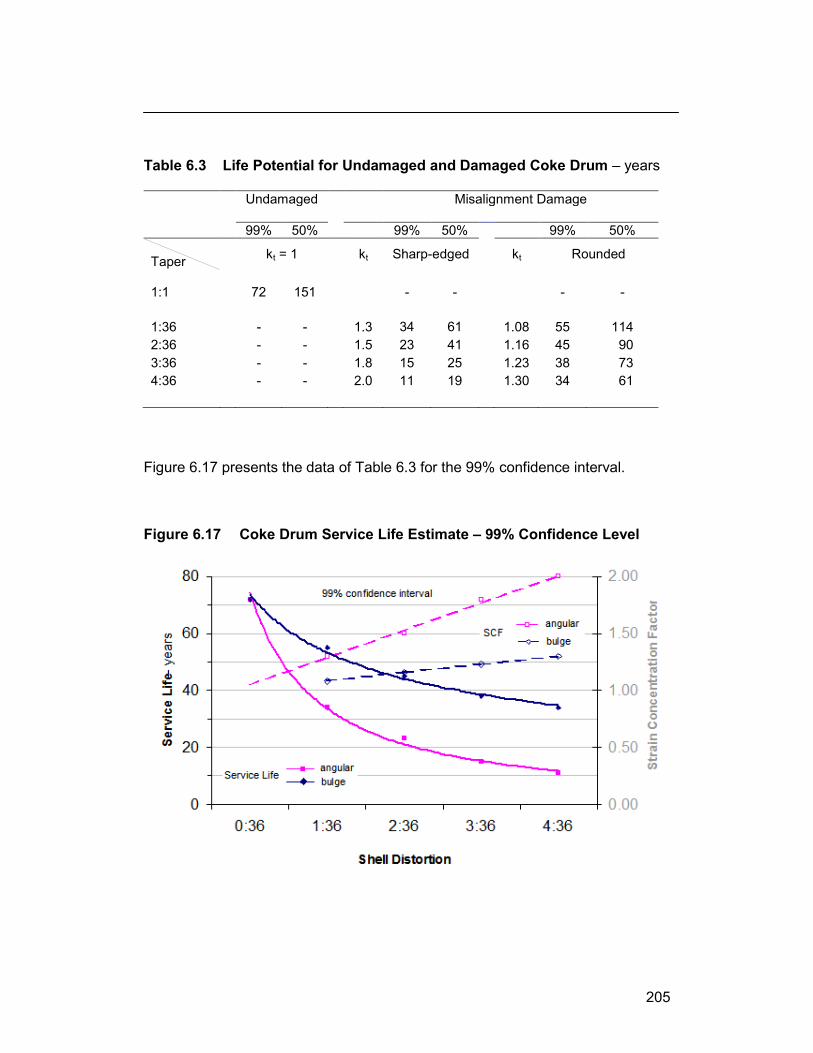
205

Table 6.3 Life Potential for Undamaged and Damaged Coke Drum – years Undamaged Misalignment Damage

99% 50% 99% 50% 99% 50%

Taper

kt = 1

kt Sharp-edged kt Rounded

1:1 72 151 - - - -

1:36 - - 1.3 34 61 1.08 55 114

2:36 - - 1.5 23 41 1.16 45 90

3:36 - - 1.8 15 25 1.23 38 73

4:36 - - 2.0 11 19 1.30 34 61

Figure 6.17 presents the data of Table 6.3 for the 99% confidence interval.

Figure 6.17 Coke Drum Service Life Estimate – 99% Confidence Level

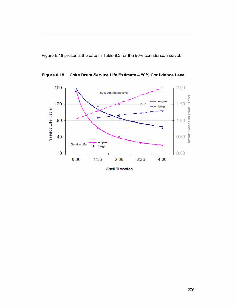
206

Figure 6.18 presents the data in Table 6.2 for the 50% confidence interval.

Figure 6.18 Coke Drum Service Life Estimate – 50% Confidence Level

207

CHAPTER 7 TEMPERATURE DEPENDENCY AND NON-LINEAR ANALYSIS

As outlined in the foregoing work, implementation of the engineering analysis

has been consistent with industry methodology so as to remain within a level of

sophistication commensurate with industry established and widely accepted

practices.

As seen, however, Code and industry methods include important

simplifications which are not sufficiently substantiated. These include

penalty factor for elastic – plastic analysis

constant valued fatigue strength reduction factor

design fatigue life approach

categorical material properties

These simplifications, if implemented by rote, preclude sufficient accuracy in

establishing a service life estimate. This thesis has addressed these four items

in detail.

The Code defers to the experience and skill of the practitioner, in a numerical

analysis, as regards the use of

temperature dependent / partially dependent material properties

linear – elastic structural analysis

non-linear – plastic structural analysis

Linear – elastic analysis is preferred for pragmatic reasons, including

simplicity in implementation

robustness, stability

efficacy

reduced run time

minimized debugging effort

suitability

In this chapter, the impact of a linear – elastic to non-linear – plastic analysis

are evaluated by using a comparative study.

208

7.1 Evaluation of Temperature Dependent Material Properties

The properties of interest using fully temperature dependent properties are

the coefficient of thermal expansion CTE, also symbolized by “"

the elastic modulus E, otherwise referenced as Young’s modulus

cyclic yield strength

The values of the CTE, i.e., and the elastic modulus directly impact the

magnitude of strain in determination of the thermo-mechanical strain, mech

arising from both the differential expansion of clad and base layers and, the

thermo-mechanical strain from self – constraint imposed between “cold spots”

and “hot spots”.

Equations (2.6) and (2.7) are repeated here for convenience:

1

1

1

)()( 0

bb

cc

chcbc

Et

Et

ETT

(7.1)

1

1

1

)()( 0

cc

bb

bhbcb

Et

Et

ETT (7.2)

For a partially temperature dependent material treatment, material properties

are treated as uniform values for the operating temperature range of interest, 100

°F to 900 °F [38 to 482 °C]. For the work described in this thesis, a temperature

of 650 °F [343 °C] was selected as a reasonable compromise.

209

Temperature dependent behaviour of CTE

The CTE values for C – ½ Mo, 1 ¼ Cr and 2 ¼ Cr alloy steels are equal, being in

the same material group according to the Code, and rise continuously. For TP

410S, the increase is less and even stationary in the vicinity of approximately 500

°F to 650 °F [260 °C to 343 °C] before increasing at a reduced rate. This results

in an increased difference in expansion between the two material groups; as a

result, as temperature increases TP 410S will experience tensile loads while the

C – ½ Mo and Cr – Mo steels will experience compressive loads, all consistent

with the expressions provided in equations (7.1) and (7.2).

Figure 7.1 CTE Values versus Temperature

Temperature dependent behaviour of the Elastic Modulus

At 650 °F [343 °C], a rapid reduction occurs in the elastic modulus, as evidenced

in Figure 7.2. For C – ½ Mo steels and TP 410S, the reduction is more rapid

than the Cr – Mo steels. At higher temperatures, material creep, a time

dependent material property becomes a consideration and has been previously

discussed in this work.

210

Figure 7.2 Young’s Modulus Values versus Temperature

Temperature dependent behaviour of Yield Strength

A material property directly affecting material selection for the construction of

coke drums is yield strength. The common construction materials are

temperature dependent as seen in Figure 7.3 where the specified minimum yield

strength [SMYS] values are plotted. The SMYS values are stipulated by Code

and provide an implicit design margin by specifying an allowable stress which

accounts for the temperature dependency of the SMYS; refer to section 1.3.4

and Table 1.3. It is commonly known in industry that these values are surpassed

by the actual yield strength [YS] of supplied materials.

211

Figure 7.3 SMYS Values versus Temperature

In addition, the SMYS values used by Code for pressure design determination

are the monotonic properties; for cyclic loading, the cyclic yield strength is the

more appropriate material property to consider. Figure 7.3 is replotted as

Figure 7.4 with the addition of the cyclic yield strength for SA 204C material

included.

212

Figure 7.4 Cyclic Yield Strength Compared to Monotonic SMYS

Noting that the cyclic yield strength of C – ½ Mo (specifically, SA 204 C) is

greater than the cyclic yield strength of Cr – Mo (specifically, 2 ¼ Cr – 1 Mo, i.e.,

SA 387 22 Class 2) at elevated temperatures and that the elastic modulus for the

former is much reduced in comparison to the latter (Figure 7.2), the observation

is made that SA 204 steels are mechanically “tougher” [30]. Hence, the apparent

better reliability observed of SA 204 steels in coke drum service.

In Figure 7.5, the cyclic strength curve for C – ½ Mo, SA 204C is provided to

illustrate its retention in cyclic strength over the temperature range of interest for

coker drum operation.

213

Figure 7.5 Cyclic Yield Strength for SA 204C at Temperature [34]

214

7.2 Application of Temperature Dependent Material Properties to Analysis

In order to assess any impact from temperature dependent material

properties and the linear – elastic structural analysis, a plane stress FEA model

was studied. The model is provided in Figure 7.6. Several model permutations

were evaluated incrementally; however, the two bounding analyses consisted of

the two approaches;

linear elastic with partial temperature dependent material properties

non-linear plastic with temperature dependent material properties Figure 7.6 Plane Stress Model for FEA Modeling Validation

Notes to Figure 7.6

1. The element used for the model is the PLANE2D 8 - node isoparametric two-dimensional plane stress for linear and non-linear analysis with

linear elastic, non – linear elasticity, plasticity, thermo-plasticity capability

two degrees of freedom (2 translations) are considered per node

one degree of freedom per node representing the temperature is used for the thermal module

2. UX, UY, UZ ≡ translational displacement; Cartesian coordinate system RX, RY, RZ ≡ rotational displacement; Cartesian coordinate system

3. Fixed support plate model, no rotation at edges 4. Parametric temperature variation from 100 °F to 900 °F [38 °C to 482 °C] 5. Temperature independent and temperature dependent material behavior used

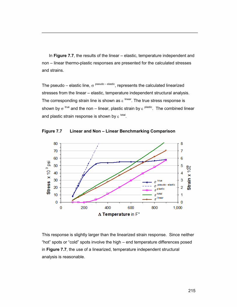
215

In Figure 7.7, the results of the linear – elastic, temperature independent and

non – linear thermo-plastic responses are presented for the calculated stresses

and strains.

The pseudo – elastic line, pseudo – elastic, represents the calculated linearized

stresses from the linear – elastic, temperature independent structural analysis.

The corresponding strain line is shown as linear. The true stress response is

shown by true and the non – linear, plastic strain by plastic. The combined linear

and plastic strain response is shown by total.

Figure 7.7 Linear and Non – Linear Benchmarking Comparison

This response is slightly larger than the linearized strain response. Since neither

“hot” spots or “cold” spots involve the high – end temperature differences posed

in Figure 7.7, the use of a linearized, temperature independent structural

analysis is reasonable.

216

This is demonstrated by examining the strain evolution of a temperature

snapshot for the shell panel studied in section five (§ 5). Figure 7.8 plots the

temperature snapshot for the linearized strain plot presented previously in Figure

5.9.

Figure 7.8 Temperature Snapshot for a Cold Spot in [°F]

Figure 7.9 plots the linearized strains from the linear – elastic, temperature

independent, composite element FEA study for the temperature snapshot

depicted in Figure 7.8.

217

Figure 7.9 Strain Report from Linear – Elastic Analysis in

Figure 7.10 plots the linearized strains from a linear – elastic FEA study for a

comparable single – layer flat plane defined by the coke drum curved shell

model. The flat plane model is required to address the limitations of the layered

element model. The figure shows the flat plane model produces near – identical

results and is slightly conservative.

218

Figure 7.10 Mechanical Strains for Linear Flat Plane Model

In Figure 7.11, temperature dependent material properties are employed to

gauge the impact of the more rigorous non-linear thermo-plastic analysis.

219

Figure 7.11 Mechanical Strains for Non – Linear Flat Plane Model

The strain results are reported in Table 7.1 for an element located in the “cold

spot” of the linear and non-linear models exhibited in Figures 7.10 and Figure

7.11 respectively. The data shows good agreement between the reported and

calculated strain results from the linear model compared to the reported results

from the non – linear model.

It can be concluded that the strain results obtained from a linear analysis can

be used to determine strains from cyclic thermal loading with sufficient accuracy

for an industry service life estimate for a coke drum shell. The practice in the

industry of using averaged mechanical properties is reasonable.

220

Table 7.1 Strain Results from Linear versus Non – Linear Models

Strain results

Model Temp stress pl

el

mech

th

total

F psi Non - linear 300 61,284 998 1,884 2,882 2,157 5,039 Linear 300 73,125 calculated – 2,823 2,823 – – reported – 2,547 2,547 – –

221

CHAPTER 8 CONCLUSIONS

The primary objective of this work was to determine the service fatigue life for

both a new coke drum and a damaged coke drum using industry practice codes

and standards. Coke drums are subject to various loadings such as internal

pressure loading, live weight loading and dead weight loading. These were

shown in previous work to be unlikely causes of shell cracking. In this work,

thermo-mechanical, low cycle fatigue cracking of the shell was shown to be the

primary damage mechanism and quantifiable in sufficient detail to allow

consequent calculation of a service life estimate for both new and damaged

drums.

There is only very limited temperature and strain data available in the few

open industry literature sources; more detailed information was provided by a

confidential source. This latter data allowed quantification of the thermo-

mechanical strains and development of a probabilistic thermo-mechanical

loading profile.

Material fatigue properties were retrieved from open literature sources and

original work conducted at the University of Alberta. These data are in excellent

agreement. Industry practices are directed to pressure vessel design; for vessels

in fatigue service, the practices establish a fatigue design life which provides an

alert for more rigorous inspections; this is especially directed to the nuclear

industry. Consequently for the problem at hand, the practices are overly

conservative and not suited for determination of practical service life estimates.

Conversely, industry practice documents contain effective and practical

methodologies which can be used, where specifically modified, to render

accurate assessments in timely and practical effort for industry use. The Code

penalty factor derived from disregarded industry research provides an accurate

method of performing simplified elastic – plastic analysis.

222

Accurate strain exposure profiles can be determined for a coke drum by

judicious and effective use of industry practice calculation methods

specific modification for use in fatigue service life determination

use of accurate fatigue strength reduction estimates

use of measured material properties

use of numerical analysis tools as outlined in this work.

Not all loading mechanisms have been discussed in this work because of the

complexity of the topic and the paucity of specific details in the open literature.

The lack of data is most likely due to the confidentiality of industry business

practices. The most damaging loading mechanism, thermo-mechanical loading

caused by significant temperature differences in adjacent portions of the coke

drum shell has been quantitatively shown to be the leading damage mechanism

contributing to shell bulging and cracking.

The following has been established in this work;

1. The service fatigue life of both a new drum and service damaged drum

can be practically determined. 2. Thermo-mechanical loading of the shell is sufficient to cause low cycle

fatigue failure in the time intervals suggested in the literature. 3. Service life is demonstrably affected by the severity of shell distortions

which unavoidably develop in service. 4. The service life and remaining life of a coke drum can be evaluated

directly by well established engineering principles and industry practices, as modified and implemented by this research work

5. The prevalent use of TP 410S cladding may be a competing source of

crack initiation especially where operational temperature exceed 850 °F [454 °C] due to creep cracking in combination with the applied thermo-mechanical loading during water quench.

223

8.1 Contributions to the Field

This work has demonstrated the practicality of making service life estimates

for coke drums by industry practitioners using accurate material properties,

industry consistent calculation methodologies and recognition of those aspects of

the calculation methodologies which are overly conservative or not adequately

suited.

This work has shown that coke drums, even though in a very severe

operational environment, have a reasonable service life when installed. As

service damage accumulates, the service life is reduced. By making an accurate

assessment of damage progression, equipment owners may better devise

operational changes and maintenance practices to preserve the integrity and

manage reliability of coke drum equipment.

224

Specifically, the contributions of this thesis can be listed;

1. that basic industry solution methodologies, as modified by this work, can

be used to determine service fatigue life estimates 2. that service fatigue life estimates can be derived for new and damaged

coke drums

3. that insight into the thermo-mechanical damage mechanism offers opportunity to modify operational and maintenance practices to optimize the service life of coke drums

4. recognition that coke drum construction materials need to be fatigue tough

5. recognition that specific thermal loading exposure profiles for coke drums

are needed to determine installation specific service life

6. demonstration that simplified linear – elastic numerical analysis is sufficiently accurate, time effective and robust to calculate thermo-mechanical loading profiles

7. that specific areas of research may be identified to further understand the design, fabrication, operation and maintenance of coke drums for more economic and safe operation of this equipment

8. that basic industry solution methodologies have been misapplied by industry practitioners, to date

9. that proxy damage criteria by industry practitioners have been and are inadequate to determine service life

225

8.2 Recommendations for Further Study

The recommendations of prior work have been completed for this effort;

however there are a number of possible research opportunities to improve the

predictive accuracy of coke drum life determination:

1. identification of alternate materials of construction for both base and clad

construction which would be better suited to high strain, low cycle fatigue failure

2. compilation of detailed data on drum operating and inspection history,

vessel condition and life retirement practices to benchmark calculation procedures

3. to investigate the impact on FSRF of weld and HAZ from alternate welded

joint fabrication technology

4. to investigate the effect Code construction allowable weld defects on shell cracking and fatigue life

5. to develop operational practices to limit shell bulging and set optimal

bulge limit criteria

6. to develop maintenance practices to remediate coke drum shell bulging damage

7. to design improved industry surveys to elicit more appropriate information and data for better engineering analysis of the coke drum bulging and cracking failure mechanisms

226

REFERENCES

1. Ellis, P.J., Paul, C.A., “Tutorial: Delayed Coking Fundamentals”, Session

Paper 29a, AIChE Spring National Meeting, March 1998, New Orleans, LA 2. Diwoky, R.J., “Continuous residuum coking by delayed coking process” ,

original article present at API meeting in Chicago, 18 Nov 1938, reprinted in 2002 by Oil & Gas Journal, Houston, TX

3. Weil, N.A., Rapasky, F.S. “Experience with Vessels of Delayed Coking Units”

Proceedings, v. 38 [III] 214-232 1958 Division of Refining, American Petroleum Institute, Washington, DC

4. Thomas, J.W. “API Survey of Coke Drum Experience” 1980 American

Petroleum Institute, Washington, DC 5. API, “Technical Report 934-G, Design, Fabrication, Operational Effects,

Inspection, Assessment and Repair of Coke Drums and Peripheral Components in Delayed Coking Units”, 1st edition, April 2016 American Petroleum Institute, Washington, DC

6. ASME, “Section VIII Division 1 Rules for Construction of Pressure Vessels”,

2010 ASME, New York, NY 7. ASME, “Section VIII Division 2 Alternative Rules for Construction of Pressure

Vessels”, 2007 ASME, New York, NY 8. API / ASME , “579 –1 / FFS –1 Fitness for Service”, 2nd Edition, 2007

American Petroleum Institute, Washington, DC and ASME, New York, NY 9. CRD Partner Information Packages; confidential information packages

provided by industry partner(s), 2003, 2007

10. “Hazards of Delayed Coker Unit (DCU) Operations”, EPA 550-F-03-001 Aug 2003 Chemical Emergency Preparedness and Prevention Office, United States Environmental Protection Agency, Washington, DC

11. ASME, “Section II Materials Part A Ferrous Material Specifications”, 2010

ASME, New York, NY

12. ASME, “Section II Part D Properties”, ASME Boiler and Pressure Vessel Code for 2010, ASME , New York, NY

13. API Proceedings “1996 API Coke Drum Survey – Final Report”, 1996 American Petroleum Institute, Washington, DC

227

14. MPC, “Coke Drum Evaluation Manual and Final Report” 1999, The Materials Properties Council, New York NY

15. Collins, J.A., “Failure of Materials in Mechanical Design – Analysis, Prediction

and Prevention”, 2nd Ed., 1993 John Wiley & Sons, New York, NY

16. British Standard, “BS 5500:1997 Specification for Unfired fusion welded pressure vessels”, 1997 The British Standards Institution, London, UK

17. Stress Engineering Services, ”2008 Coke Drum Seminar”, September 2008

Stress Engineering Services Inc., Houston TX

18. Ramos, A., Rios, C.C., Vargas, J., Tahara, T., Hasegawa, T., “Mechanical Integrity Evaluation of Delayed Coke Drums”, PVP volume 359 1997: 291-298 ASME, New York, NY

19. Ramos, A., Rios, C.C., Vargas, J., Johnsen, E., Gonzalez, M., “Delayed

Coking Assessment Using Field Measurements & FEA”, PVP volume 368 1998: 231-237 ASME, New York, NY

20. Penso, J.A., Lattarulo, Y.M., Seijas, A.J., Torres, J., Howden, D., Tsai, C.L.,

“Understanding Failure Mechanisms to Improve Reliability of Coke Drums”, PVP volume 395 1999: 243-253, ASME, New York, NY

21. Boswell, R.S., Farraro, T., Sober, M.J., “Remaining Life Evaluation of Coke

Drums”, 1997 Energy Week Conference and Plant Engineering, Operations, Design & Reliability Symposium, ASME / API, Houston, TX

22. Church, J.M., Lim, L.B., Brear, J.M., Jarvis, P., Lant, R.P.D., Middleton, C.J.,

“Crack growth modeling and probabilistic life assessment of coke drums operating under fatigue conditions”, International Journal of Pressure Vessels and Piping, v 78 2001:1011-1020, Elsevier Science Ltd., Amsterdam, Netherlands

23. Boswell, R.S., Wright, B., “State-of-the-Art Improvements in Coke Drum

Design and Life Extension Practices”, CREEP 2007 – 26254, Proceedings of CREEP8, 8th International Conference on Creep and Fatigue at Elevated Temperatures, July 2007, ASME, San Antonio, TX

24. Ohata, M., Kawai, N., et al., “Investigation of Bulging Behavior of Coke Drum

– Feasible Study on Causes of Bulging”, PVP2011 – 57276, Proceedings of the ASME 2011 Pressure Vessels & Piping Division Conference, Baltimore, MD

228

25. Yamamoto, T., Arii, K., et al., “Investigation of Bulging Behavior of Coke Drum – A Practical Analysis of Bulging Under Complex Quench Conditions”, PVP2011 – 57428, Proceedings of the ASME 2011 Pressure Vessels & Piping Division Conference, Baltimore, MD

26. Samman, M., Samman, M., “Stress Analysis of Bulges in Cylindrical and Oval

Pressure Vessels”, PVP2014 – 28138, Proceedings of the ASME 2014 Pressure Vessels & Piping Division Conference, Anaheim, CA

27. Samman, M., Tinoco, E.B., Marangone, F.C., “Comparison of Stress and

Strain Analysis Techniques for Assessment of Bulges in Coke Drums”, PVP2014 – 28139, Proceedings of the ASME 2014 Pressure Vessels & Piping Division Conference, Anaheim, CA

28. Samman, M., DuPlessis, P., “The Bulging Intensity Factor (BIF™), A

technique for assessing the bulging severity of coke drums”, RMC-07-100 2007 NPRA Reliability & Maintenance Conference, NPRA Houston, TX

29. Barsom, J.M., Vecchio, R.S., “WRC Bulletin 432 Fatigue of Welded

Structures” June 1997 Welding Research Council, New York, NY

30. Harvey, J.F., “Theory and Design of Pressure Vessels”, 1985 Van Nostrand Reinhold Company, New York, NY

31. Aumuller, J., “Aspects of the Thermo Elasto-Plastic Response for a Coke

Drum under Cyclic Loading” M. Sc. Thesis 2009, University of Alberta, Edmonton, Alberta

32. J.H. Gross, “WRC Bulletin 101 PVRC Interpretive Report on Pressure Vessel Research, Section 2 – Materials Considerations“ Nov 1964 Welding Research Council, New York, NY

33. Dowling, N.E., ”Mechanical Behaviour of Materials – Engineering Methods for Deformation, Fracture, and Fatigue”, 4th Ed., 2013 Pearson Education Prentice Hall, Upper Saddle River, NJ

34. Chopra, O.K., Shack, W.J., “Low-cycle fatigue of piping and pressure vessel

steels in LWR environments” volume 184 (1998) pp. 49 – 76 Nuclear Engineering and Design, Elsevier Science S.A., Amsterdam, Netherlands

35. Chen, J., “Fatigue Behavior of Coke Drum Materials and Its Application to

Extend the Service Lives of Coke Drums”, Ph. D. Thesis 2014, University of Alberta, Edmonton, Alberta

229

36. Jaske, C.E., Hechmer, J.L., “WRC Bulletin 422 Fatigue Strength Reduction Factors for Welds in Pressure Vessels and Piping” June 1998 Welding Research Council, New York, NY

37. Araque, E.D., Vivas, G.A., Moret, A.J., Bello, R.E., “Fitness for Service

Evaluation of a Bulging Coke Drum”, PVP2015– 45190, Proceedings of the ASME 2015 Pressure Vessels & Piping Division Conference, Boston, MA (not included in official publication of conference proceedings)

38. Zhang, Y., Xia, Z., “Simplified Thermo-elasto-plastic Analysis Models for

Determination of Global and Local Stresses in Coke Drums”, PVP2013 – 97296, Proceedings of the ASME 2013 Pressure Vessels and Piping Conference, Paris, France

39. Beckwith,T.G., Buck, N.L., “Mechanical Measurements”, 2nd Edition 1973

Addison Wesley, Reading, MA

40. TML, “Strain Gauges Catalog Pam E – 1007A” pg 14 Tokyo Sokki Kenkyujo Co., Ltd., Tokyo, Japan

41. ASTM, “E 8 – 04 Standard Test Methods for Tension Testing of Metallic

Materials”, 2004 ASTM, West Conshohocken, PA

42. Gray, T.G.F., Spence, J., North, T.H., “Rational Welding Design”, 1975 Newnes – Butterworths, London, UK

43. Manson, S.S., “Thermal Stress and Low-Cycle Fatigue”, 1966 McGraw-Hill

Inc., New York, NY

44. Langer, B.F., “Design of Pressure Vessels for Low-Cycle Fatigue”, vol 84 iss 3 pp. 389 – 399 1962 ASME Journal of Basic Engineering, New York, NY

45. Coffin, L.F., “A Study of the Effects of Cyclic Thermal Stresses on a Ductile

Metal”, Trans. ASME vol. 76, p 931 1954 ASME, New York, NY

46. Tavernelli, J.F., Coffin, L.F.,”A Compilation and Interpretation of Cyclic Fatigue Tests on Metals”, vol. 51 p 438 1959 Trans. ASM, American Society for Metals, Materials Park, OH

47. Manson, S.S., Hirschberg, M.H., “The Role of Ductility, Tensile Strength and

Fracture Toughness in Fatigue”, vol 290 pp 539 – 548 no. 6 1970 The Journal of the Franklin Institute, Philadelphia, PA

48. ASME, “Criteria of the ASME Boiler and Pressure Vessel Code for Design by

Analysis in Sections III and VIII Division 2” 1969 ASME, New York, NY

230

49. Jaske, C.E., “Materials-Data Needs for Fatigue of Pressure Vessel Systems”, pp.600 - 611 Low Cycle Fatigue and Life Prediction, 1982 ASTM STP 770, Amzallag, C., Leis, B.N., Rabbe, eds., Philadelphia, PA

50. Jaske, C.E., in “Thermal-Mechanical, Low Cycle Fatigue of AISI 1010 Steel”,

Thermal Fatigue of Materials and Components, 1976 ASTM STP 612, pp 170 – 198, Spera, D.A., Mowbray, D.F., eds, ASTM, Philadelphia, PA

51. Manson, S.S., “A Simple Procedure for Estimation High-temperature Low-

cycle Fatigue” 5 (7) pp. 349 – 355 1968 Experimental Mechanics, Springer, Society for Experimental Mechanics, Bethel, CT

52. Manson, S.S., “ Some Perspectives on Future Directions in Low Cycle

Fatigue”, Low Cycle Fatigue, 1988 ASTM 942, pp 5 - 14, H. D. Solomon, G. R. Halford, L. R. Kaisand, and B. N. Leis, eds., American Society for Testing and Materials, Philadelphia, PA

53. Kalnins, A., Dowling, N.E., “Design Criterion of Fatigue Analysis on Plastic

Basis by ASME Boiler and Pressure Vessel Code”, 126 pp. 461 – 465 2004 Journal of Pressure Vessel Technology, ASME, New York, NY

54. O’Donnell, W.J., “§ 39, Code Design and Evaluation for Cyclic Loading – Sections III and VIII”, Companion Guide to the ASME Boiler & Pressure Vessel Code,2nd Edition, 2006, ASME, New York, NY

55. Stephens, R.I., Fatemi, A., Stephens, R.R., Fuchs, O.H., “Metallic Fatigue in Engineering”, 2nd Edition, 2001 John Wiley & Sons, New York, NY

56. Kreith, F., “Principles of Heat Transfer”, 3rd Ed., Intext Press Inc., 1973 New

York, NY

57. Kelkar, V.S., Sewell, R.T., “Fundamentals of the Analysis & Design of Shell Structures”, 1987 Prentice Hall Inc., Englewood Cliffs, NJ

58. ASTM, “E 1049 – 85(2011) Standard Practices for Cycle Counting in Fatigue

Fatigue Analsysi”, 2011 ASTM International, West Conshohocken PA

59. “World Class Coke Drum Replacement”, http://nooterconstruction.com/world-class-coke-drum-replacement-el-secundo-chevron-nooter/ accessed 24 Oct 2016

60. API, “API Standard 650 Welded Tanks for Oil Storage”, 12th Edition, March

2013 American Petroleum Institute, Washington, DC

231

61. Boswell, R. S., Farraro, T.D., “Method of Designing and manufacturing a delayed coke drum”, US Patent 5,827,403 granted 27 October 1998, Alexandria, VA

62. ASME, “Section VIII Division 3 Alternative Rules for High Pressure Vessels”,

2007 ASME, New York, NY

63. Slagis, G.C., “Meaning of Ke in Design-by-Analysis Fatigue Evaluation”, [128] Feb 2006, Transactions of the ASME, ASME, New York, NY

64. Krempl, E., “Notched High-Strain Fatigue Behavior of Three Low-Strength

Structural Steels” General Electric Report GEAP-5714 1969, Atomic Power Equipment Department, General Electric, San Jose, CA

65. Lang, H., Rundolph, J., Ziegler, R., “Performance study of Ke factors in

simplified elastic plastic fatigue analysis with emphasis on thermal cyclic loading”, 88 2011 pp 330 – 347 International Journal of Pressure Vessels and Piping, Elsevier B.V., Amsterdam, Netherlands

66. Wundt, B.M., ed. “Fatigue Strength Reduction Factors in Bending”, ASTM

STP 490 Effect of Notches on Low-Cycle Fatigue, A Literature Survey, 1972 pp 29 – 44, ASTM, Philadelphia, PA

67. ASME, “B31.7 - 1969 Nuclear Power Piping”, 1969 ASME, New York, NY

68. Langer, B. F., “Design-Stress Basis for Pressure Vessels,” Pressure Vessel

and Piping: Design and Analysis, A Decade of Progress, Volume 1, pp. 84 – 94, 1972 ASME, New York, NY

69. Gerber, T. L., “Effect of Constraint and Loading Mode on Low-Cycle Fatigue

Crack Initiation—Comparison with Code Design Rules,” General Electric Report GEAP-20662 1974, Atomic Power Equipment Department, General Electric, San Jose, CA

70. Iida, K., Kitagawa, M., Tamura, K., Matsushita, A., Fukagawa, M., and Saiga,

Y., “Safety Margin of the Simplified Elasto Plastic Fatigue Analysis Method of ASME B and PV Code Section III,” 1980, Institution of Mechanical Engineers, London, UK