ISSN: WEIGHTING CUSTOMERS’ DATA FOR MORE … · forecast model in the electrical system with the...

Journal of Theoretical and Applied Information Technology 31

st August 2016. Vol.90. No.2

© 2005 - 2016 JATIT & LLS. All rights reserved.

ISSN: 1992-8645 www.jatit.org E-ISSN: 1817-3195

23

WEIGHTING CUSTOMERS’ DATA FOR MORE ACCURATE

SHORT-TERM LOAD FORECAST

1SYLVIA JANE A. SUMARAUW,

2SUBANAR,

3EDI WINARKO,

4RETANTYO WARDOYO

1 Computer Science Doctoral Program, Faculty of Mathematics and Natural Science, Universitas Gadjah

Mada 2 Department of Mathematics, Faculty of Mathematics and Natural Science, Universitas Gadjah Mada 3,4

Department of Computer Science and Electronics, Faculty of Mathematics and Natural Science,

Universitas Gadjah Mada

E-mail: [email protected],

[email protected],

[email protected],

[email protected]

ABSTRACT

Disruption of the electricity supply service to the customers or the overload primary energy usage is often

caused by load forecast fault. This fault, especially the short-term load forecast (STLF), occurs by

unpredictable factors. One of these factors is weather effect in a load centre.The application of the load

forecast model in the electrical system with the use of energy trend on the demand site, influenced by

fluctuations of the weather, requires weather data from the affected electrical system areas. However,

weather stations in Indonesia are limited and do not represent the electrical system areas. Although STLF

research used many methods has been widely conducted in many countries, Indonesia, especially PLN

(national electrical company, the only electricity provider in Indonesia) has not undertaken it. Moreover,

the studies that clearly explain the coverage areas of the electrical system and how to obtain the weather

data have not yet been conducted. This paper discusses a method in obtaining the weather data through

weather observation sites represented the load centres in the coverage areas of electrical system. The result

shows that the application of the method improved the forecasting performance.

Keywords: Short-Term Load Forecast (STLF), Load Forecasting, Weighting Customers, STLF Weather

Sensitive, STLF Trends

1. INTRODUCTION

Electricity is a unique product because it cannot

be stored in large quantity and is only produced

when needed. Producing intensive electricity

technology into a highly beneficial product needs

efficient production, a proper production technique

and a highly multidiscipline involvement as well, to

generate a low cost production. In operational

practices in most countries, technical arrangements

and load distributions of the electrical systems have

to be managed by a unit of organisation using the

best practice applications and techniques in

electricity energy. The electrical system discussed

is the system of extra high voltage electrical

network (>150kV) is integrated in an

interconnection system and exclusively managed by

a manager unit. Operating procedures play essential

role in determining the production cost and the

reliability of the system. This is important because

mistakes of operation pattern, especially in primary

energy source usage, can result in substantial

losses. Planners use loading forecast as a basic

analysis in determining the operational patterns.

The disruption of electricity supply services to

the customers or the excessive primary energy

usage is often caused by the unpredictable factors.

The initial exploration results found some

phenomena which suggested that one of the causes

is the weather of the load centre site. This leads to

an inapt load forecast. Another obstacle is the

limited weather stations in Indonesia to cover the

whole electrical system areas.

A lot of research on STLF weather sensitive has

been conducted [1]-[17]. Several STLF studies used

case studies in some countries, for example Greece

[12], Kuwait [3], Spain [19], Ireland [7], Slovakia

and North America [24], Japan [25], United State

of America [26], China [27], India [28], [29],

Finland [30], Nigeria [31], and Malaysia [9], [32].

The weather sensitive model is usually

implemented for electrical system, in which the

energy usage at a demand site has a tendency to be

influenced by weather fluctuation. The main





24

difficulty of the application of this model is the way

of obtaining the weather prediction data to

represent the electrical system. No research has

explained clearly the coverage area of the electrical

system and the way of obtaining it.

A lot of STLF research has been conducted in

many countries, but donly few studies have been

performed in Indonesia. Most of the studies faced

the vast and diverse of Indonesian geography, as

the result, the STLF studies were specified for each

area. The implementation of STLF in Indonesia,

especially by PLN, is limited. Every country is

affected by a different electricity demand.

Moreover, in some developing countries such as

Indonesia, the electricity forecast growth increases

dynamically. Therefore, every electric network

needs a unique forecast method [3]. The past study

method that used weather cannot be implemented in

Indonesia due to different conditions of season and

completeness of weather data. An inaccurate

weather data involvement in a study may lead to an

imprecise weather forecast result [33].

Deoras (2010) conducted research on the

electrical system in the Nepool region, United

States, produces an error of 1-2%. Apparently,

testing of this using the data electrical systems in

South Sulawesi, Indonesia, produces a greater error

(~3.35%). The error is possibly caused by the

weather condition. The weather condition used for

the testing is only from one weather station namely,

the Sultan Hasanuddin International Airport

weather station. This study develops a method of

weighting customer data to improve the value of

the original weather data only from one station

observation. This data can represent area electricity

system and provide more accurate forecasting

performance (~ 2.91%).

2. BACKGROUND

Based on literature reviews, some of the notes

are as follows:

− The models that were developed and tested were

basically specific for the developed electrical

system. The developed models were not able to

be implemented without reviewing and testing.

These related to the used parameters.

− The use of input variable weather data from

STLF studies is one of the main variables,

especially in areas where the dynamics of

seasonal patterns are generated with difficulty.

− Generally, weather sensitive research is not

troubled by the weather data and weather

forecast obtained on the forecast day because the

characteristic of demand site behaviour can be

predicted easily. On the contrary, it is very

different from Indonesia or any tropical climate

areas, where the weather changes might lead to

changes in customer behaviour in consuming

electricity.

− Most of the previous electrical system studies

have a quite large coverage area, dense

populations, easily obtained weather data and in

a flat condition.

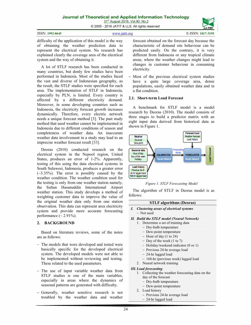
2.1. Short-term Load Forecast

A benchmark for STLF model is a model

research by Deoras (2010). The model consists of

three stages to build a predictor matrix with an

eight input data derived from historical data as

shown in Figure 1.

Figure 1. STLF Forecasting Model

The algorithm of STLF in Deoras model is as

follows:

STLF algorithms (Deoras)

I. Clustering areas of electrical systems

− Not used

II. Build the STLF model (Neural Network)

1. Determine a set of training data

− Dry-bulb temperature

− Dew-point temperature

− Hour of day (1 to 24)

− Day of the week (1 to 7)

− Holiday/weekend indicator (0 or 1)

− Previous 24-hr average load

− 24-hr lagged load

− 168-hr (previous week) lagged load

2. Neural network training

III. Load forecasting

1. Collecting the weather forecasting data on the

day of the forecast



2. Load history







25


3. Weekend indicator of the day of forecast

4. Load forecasting results

2.2. Forecasting using weather information

To overcome the weather differences in an

electrical system area, there should be a study of

methods on how to obtain weather data from a

weather station that becomes the weather data from

the coverage area which represents the electrical

system. This paper offers a method to get weather

data through some weather observation points

representing the load centres in the coverage area of

the electrical system. The weather data is used as an

input of STLF forecasting.

3. PROPOSED METHOD

The data consists of weather data, load data,

customer data, and geospatial data of the

subscribers on electrical systems of the PLN in

South Sulawesi, Southeast Sulawesi and West

Sulawesi, Indonesia. The data was retrieved from

the period of January 1, 2007 to December 31,

2013. The data from 2007 to 2012 was used as

training data and the data in 2013 was used as the

test data.

The stations of weather observation that were

included in the electrical system coverage were

very limited. The history of weather data that can

be obtained from the "weatherspark" website, donly

lists the observation station at the Sultan

Hasanuddin International Airport, Makassar,

Indonesia. This study proposes method to get the

value of weather data that can represent the

coverage of the electrical system. In achieving the

objectives, several assumptions and optimizations

used are as follows:

− The customer behaviour towards weather

fluctuations is classified based on customer

segmentation, namely: industrial and business

customers, government customers, household

customers, and others.

− Customer data is defined using a unique

identifier and can be distinguished intake of

energy consumption that comes from an

electrical system or an isolated system.

− As the organizer of electricity supply in

Indonesia, the PLN is in transition for

implementation of the map-based information

systems or geographic information systems. The

implication is that each customer has geospatial

data as a customer site. Implementation of new

service products such as prepaid electric meter

requires a completion geospatial data of

customers. Moreover, GIS is also useful to

measure electrical consumption by the

conventional electrical meter costumers.

Based on customer classification, the example of

behaviour each customers segment to the different

weather fluctuations, can be seen as form follows:

− In the industrial segment in general, weather

fluctuations do not affect the production and the

machines will continue to operate. However, in

certain industries like rice mills and ice factories,

weather fluctuations have a great impact on the

production capacity. They affect the use of

electricity as the driver of production engine.

− In the government and households segment, the

tendency of energy use is similar, for example

the use of work/home appliances such as air

conditioner (AC), humidity control equipment,

lighting, and others. On weekdays and holidays

between government and household segments, it

is inversely proportional.

Classification of customers or customer

segmentation needs to be considered because every

customer has different ratios that show significant

impact on the load consumption of the electrical

system. The studies on the subject are studied and

formulated into a weight value customer who is

associated with an installed power of the customer.

Based on geospatial data held for each customer,

the distribution centres and the load on the

electrical system coverage can be seen. This

information is used to divide the electrical system

into clusters and cluster centre, so that the location

where the weather data is needed can be

determined. Customer behaviour in consuming

electrical energy is associated with weather

conditions. Meanwhile, the weather conditions

depend on location, so that the approach to the

weather data input to STLF is weather data where a

customer is located.

The division of the load centres into several

segments uses k-means clustering technique. The

weather is assumed to be valid up to a radius of 40

km. The covering area of electrical systems by

using a circle can be done as shown in Figure 2 and

Figure 3.





26

Figure 2. Cover The Area

With Overlapping Circles

Coincide

Figure 3. Cover The Area

With Circles Without An

Area That Is Not Covered

− Figure 2 is about how to cover an area using a

circular where the circles will fill the area with

the most efficient way and the sides of the circle

coincide with each other. This method has a

drawback because there is area that is not

covered.

− Figure 3 is about the best way to cover the area

using circles where the radius of the circle used

is the minimum. This method ensures that there

are only a few areas that can be covered

maximally by only two circles. Figure 3 uses a

radius of 40 km (the same as the assumptions

used).

− The circles in Figure 2 will be used to calculate

how many circles are needed to meet the area of

the electrical system.

Figure 2 and Figure 3 combined in a same area

(reference area used = the electrical system) will

look like Figure 4. The lack areas covered using

Figure 2 can be addressed using the index/ratio

multiplier with the concept described in Figure 4.

Figure 4. Illustration Of A Circle That Covers An Area

From the left bottom of Figure 2 the following

relations obtained:

X = 40 cos 30°� Area of a circle with a radius

of X km = A

� � �� 40 �� 30°��

The field of the electrical system = Number of area

local governments on the electrical system=AES

��

��

4��

��

4

�

The number of clusters is calculated as follows

� �4

��

��

� � �40 � cos 30°��

�4��

�40 � � � cos 30°��

The next step is to use k-means clustering.

K-means clustering algorithm is shown in Figure 5.

Centre weighted cluster aims to come closer to the

centre of the cluster of potential data/information.

The weight of the customer data as information is

power potential customers. The method of

calculating the weighted cluster centres uses "centre

of mass" calculation formula and is defined as

follows:

#$ �∑ &' . )'

*'+,

∑ &'*'+,

, #. �∑ &' . /'

*'+,

∑ &'*'+,

where,

Cx = longitude coordinates of the center of the

cluster

Cy = latitude coordinates of the center of the

cluster

Pi = power installed on the ith

customer (VA)

xi = ith

customer locations in longitude

coordinates

yi = ith

customer locations in latitude

coordinates

The number of clusters from the calculation is N

= 8, and the clustering process is done by using the

value of the latitude, longitude, and power

customers.





27

Figure 5. Kmeans Clustering Algorithm

Centre cluster as pairs of values (x, y) is in the

form of a matrix 8 x 2. The results calculated by

weighting the central cluster are shown in Table 1.

Table 1. The Centers Of Clusters As A Result Of The

Weighting

Number Coordinate

point East

Longitude South

Latitude

1 C1 120.0510 3.0123

2 C2 120.0626 4.3555

3 C3 120.1874 3.6669 4 C4 119.6763 3.7866

5 C5 119.7966 4.7986 6 C6 119.4642 5.1419

7 C7 120.1290 5.3247

8 C8 119.6981 5.4676

Cluster centers if drawn on a map is shown in

Figure 6.

Figure 6. The Centers Of Clusters With Weighting

STLF proposed model design requires 9 input

data, IE

(1) Dry-bulb temperature

(2) Dew-point temperature

(3) Humidity

(4) Hour of day (1 to 48)

(5) Day of the week (1 to 7)

(6) Holiday/weekend indicator (0 or 1)

(7) Previous 24-hr average load

(8) 24-hr lagged load

(9) 168-hr (previous week) lagged load

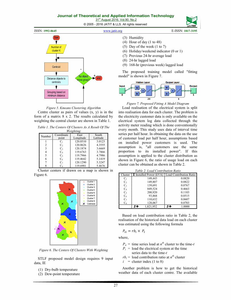
The proposed training model called "fitting

model" is shown in Figure 7.

Figure 7. Proposed Fitting A Model Diagram

Load realisation of the electrical system is split

into realisation data for each cluster. The problem is

the electricity customer data is only available on the

electrical system log data collected through the

activity meter reading which is done conventionally

every month. This study uses data of interval time

series per half hour. In obtaining the data on the use

of customer load per half hour, assumptions based

on installed power customers is used. The

assumption is, "all customers use the same

proportion to its installed power". If this

assumption is applied to the cluster distribution as

shown in Figure 6, the ratio of usage load on each

cluster can be obtained as shown in Table 2.

Table 2. Load Contribution Ratio Cluster Σ Installed Power (kVA) Load Contribution Ratio

C1 149,443 0.0820

C2 149,807 0.0822 C3 139,691 0.0767

C4 849,524 0.4663

C5 200,920 0.1103 C6 93,868 0.0515

C7 110,632 0.0607

C8 128,067 0.0703

Σ� 1,821,952 Σ� 1.0000

Based on load contribution ratio in Table 2, the

realisation of the historical data load on each cluster

was estimated using the following formula

&0' � �1' �&0

where,

Pti = time series load at nth

cluster to the time-t

Pt = load the electrical system at the time

series data to the time-t

rbi = load contribution ratio at nth

cluster

i = cluster index (1 to 8)

Another problem is how to get the historical

weather data of each cluster centre. The available





28

historical weather data that can be obtained is only

from one weather observation station. Using

weather data from the weather observation stations

of Sultan Hasanuddin Airport in Makassar for the

entire cluster centre location is not suitable and

opposed to the presumption of this study. In

obtaining the necessary data to reach the expected

goals, some considerations are needed to be

applied. First, consider the geographical conditions

of each cluster centre, which is the altitude

correlated to temperature and air density. In this

case, the altitude is the elevation scale measured

against a reference datum, the sea surface (sea

level). The geographic data altitude in each cluster

can be seen in Table 3.

Table 3. Altitude Cluster Centers

Number Cluster East

Longitude

South

Latitude

Altitude

(m) 1 C1 120.0510 3.0123 1314 2 C2 120.0626 4.3555 119

3 C3 120.1874 3.6669 515

4 C4 119.6763 3.7866 13 5 C5 119.7966 4.7986 534

6 C6 119.4642 5.1419 14

7 C7 120.1290 5.3247 483 8 C8 119.6981 5.4676 445

Note: Sultan Hasanuddin International Airport is located in cluster number 6 with an elevation of 14 m, and the weather conditions at the center of the cluster C6 are considered equal.

In a simple, correlation between temperature and

altitude can be stated that every increase in altitude

of 1000 m, lowers the temperature by 9.8 °C (if the

conditions are sunny/dry) and 6 °C (in cloudy

conditions). In cloudy weather conditions, any

increase in altitude of 1000 m make the temperature

drops by 6 °C (Quoted from the website at the

website address http://www.onthesnow.com/news/

a/15157/ask-a-weatherman--how-does-elevation-

affect-temperature- [Accessed January 24, 2016]).

Thus dry bulb temperature on each cluster center

can be determined as follows

23 � The temperature data on weather observation

stations (Sultan Hasanuddin International

Airport)

2, � 23 4 3�567,8�

,999� 23 4 7.8

2� � 23 4 3�5<7,8�

,999� 23 4 0.63

2> � 23 4 3�5?7,8�

,999� 23 4 3.01

28 � 23 4 3�5A7,8�

,999� 23 B 0.01

2C � 23 4 3�5D7,8�

,999� 23 4 3.12

2F � 23 4 3�5G7,8�

,999� 23 4 2.81

2H � 23 4 3�5I7,8�

,999� 23 4 2.59

Humidity at a site is also influenced by the

density of the air that is correlated with altitude. Air

density indicates the compactness of air molecules

and directly proportional to the humidity. Table 4

shows the relationship between the ratio of density

of air and altitude. Based on the relationships

presented in Table 4, the data humidity on each

cluster can be determined as follows:

L3 � humidity data in weather observation stations

(Sultan Hasanuddin International Airport)

L, � L3 B 0,1390

L� � L3 B 0,0116

L> � L3 B 0,0785

L8 � L3 B 0,0013LC � L3 B 0,0803

LF � L3 B 0,0754

LH � L3 B 0,0718

Table 4. The Relationship Between The Ratio Of The Air

Density And Altitude

Altitude Air Density Ratio (At Altitude/At Sea Level)

Temperature (Deg F) Feet Meter

Sea Level 0 1 59

1000 304.8 0.9702 55.4

2000 609.6 0.9414 51.9 3000 914.4 0.9133 48.3

4000 1219.2 0.8862 44.7

5000 1524.0 0.8598 41.2 6000 1828.8 0.8342 37.6

Exterior Ballistics quoted from the website at the website address http://www.exteriorballistics.com/ebexplained/5th/31.cfm

The next weather data is dew-point which can be

calculated based on the previous observation of the

temperature and humidity parameters. The

formulations for calculating the Dew Point is as

follows

DPOP � TOP B�100 B HOP ∗ 100�

5

where,

DPti = dew-point time series data at cluster-i

for the time-t

Tti = temperatur time series data at cluster-i

for the time-t

Hti = humidity time series data at cluster-i

for the time-t


The proposed method uses training data

consisting of the data of the load on each cluster (8

clusters, each one packet of data load time series),

and weather data from each cluster center (8

locations), each of which consists of three packages

weather data time series (Figure 8).





29

Figure 8. Proposed STLF Forcasting Model

STLF forecasting algorithms proposed are as

follows

Proposed STLF forecasting algorithm

I. Clustering areas of electrical systems

1. Finding and calculate the area of the electrical

system (AES)

2. Calculating the number of clusters, � �8TUV

�89�W�XYZ>9°�<

3. Clustering using k-means clustering to generate

the cluster members.

4. Looking cluster centers using weighting (center

of mass), where each center cluster i (i = 1 to n)

is calculated according to the following formula

#$ �∑ [\.$\]\^6

∑ [\]\^6

, #. �∑ [\..\]\^6

∑ [\]\^6

5. Looking altitude at each center cluster on a map

(h1, h2, ....., hi, ....., hn), where i = 1 to n

6. Calculate the load contribution ratio on each

cluster (rb1, rb2, ....., rbi, ....., rbn), where

�1' �∑_`\

∑_`abc , and

Σ DTi = The total number of installed power

customers in cluster-i

Σ DTTot = The entire number of installed

power customers in cluster-i

i = 1 to n, and, for rbi effect relationship ∑ �1'

*'+, � 1

7. Menghitung beban pada setiap cluster (P1,

P2, ....., Pi, ....., Pn),

&0' � �1' �&0 , where

Pti = time series load at nth cluster to the

time-t

Pt = load the electrical system at the time

series data to the time-t

rbi = load contribution ratio at nth cluster


II. Building the STLF model (Neural Network)

1. Determine a set of training data

for i = 1 to n

− Dry bulb temperature �2' � T3 43�de7,8�

,999

− Humidity (Hi)

select case i

case 1: C= 0.1390

case 2: C= 0.0116

case 3: C= 0.0785

case 4: C= 0.0013

case 5: C= 0.0803

case 6: C= 0

case 7: C= 0.0754

case 8: C= 0.0718

end select

Hi = H6 - C

− Dew-point temperature,

f&' � 2' B�100 B L' ∗ 100�

5

− Hour of day (1 to 48)

− Day of the week (1 to 7)

− Holiday/weekend indicator (0 or 1)

− Previous 24-hr average load (L1i)

− 24-hr lagged load (L2i)

− 168-hr (previous week) lagged load (L3i)

next i

2. Neural network training

III. Loading forecast

1. Collecting the weather forecasting data on the

day of the forecast



− Humidity

2. Load history




3. Weekend indicator of the day of forecast

4. Load forecasting results

4. RESULTS AND DISCUSSION

Deoras claimed an accuracy of 1-2% in his

research, but in this research the data produced a

3.35% accuracy. The existence of these differences

can be explained as follows. Firstly, analyzing the

model, especially on parameters that build the

model. In this case, the forecasting results are

determined by the predictor matrix, where Deoras

used eight inputs in forecasting models. Secondly,

models of time series data that can be analyzed are

the load historical data time series and weather data

time series. Load historical data time series do not

matter anymore because the data is historically

valid for both in the Nepool and in the PLN. One

type of data again is the time series data of weather

which is typically different between the two regions

(Nepool and South Sulawesi). In the Nepool, the

working area of service is quite extensive, but the

typical climate in the area tends to be the same. In

Indonesia, it is likely that the weather conditions

are very volatile.





30

Although no real data can be shown, but from the

logic on the results obtained it can be concluded

that the historical data as a weather forecasting

model builder in network training process in

building the model is the main factor affected such

differences. In other words, the weather history data

at the Sultan Hasanuddin International Airport, as

the only weather data that can be obtain and the

electrycal system that is used in this research,

produces a less good forecasting model (MAPE =

3.35%). If the model is expected to provide

sufficient level of accuracy forecasting, we need to

develop the method to obtain weather data in

another location or multiple locations which can

represent the electrical system. At every level of the

climate, it will significantly affect the tendency of

electricity consumption in the region.

This study focused on the weather as a major

factor, besides of course the historical exploitation

of data. In achieving the desired level of

performance forecasting, several other factors other

than weather data that represent the areas of

electrical systems need to be considered the method

to develop. An essential factor is data quality. Data

is not only time-series data as input in forecasting

models, but also the quality of data for architectures

that build the overall system. One data that plays a

major role in achieving the desired level of

performance forecasting particularly if the proposed

method is the identity data of the customer, which

in this case is the customer geospatial data. The

available geospatial data in this study is only

19.1%, and the 80.9% of the data is the randomly-

generated geospatial data. Although in generating

the geospatial data the research used a boundary

layer approach to the city administration on a map

and city data contained in the subscriber's identity,

but these influenced the overall forecasting

accuracy.

The proposed model needs a model design

accuracy and a required parameters as input to the

forecasting model. One of the ideal conditions is

the quality of the data that establish is the overall

system architecture. The availability of geospatial

data of customers is one of the things that provides

accuracy of getting data from the clusters centres

with a weighting of customer data. Another

relevant ideal condition in supporting the accuracy

of forecasting is by negating the assumptions

related to the determining of the values predicted in

the cluster, such as historical data load on each

cluster, and the weather data in each cluster. The

limitation of this study is that after the formation of

the cluster, there is no real historical data on the

cluster that can be used (such as historical data load

on the cluster). Therefore, this study have to use the

approach through the load contribution ratio.

The main concept of the proposed method is to

get the weather data that represens the electrical

system through the distribution area of the electrical

system into several clusters. The distribution of the

cluster does not have to use methods such as k-

means applied in this research, but what need to be

repaired is segmentation in the area of the electrical

system and any existing segments have a data

logger that can be accessed as time series data.

Support existence of IT to create ideal conditions

plays an important role. Data logger on SCADA

systems is an operational technology (OT), while

the geospatial data of customers and identity data of

customers is the information technology (IT). Both

of which have different characteristics (see Table

5), and the convergence between the two is a

strategy that needs to be done. Actualising the ideal

conditions requires a stage, and cannot be forced.

For example, to get the required customer survey

geospatial data to customers, and of course not only

the location of the customer must be in the survey,

but including the distribution assets of customers,

and this requires a considerable cost. It is not a cost

issue, but the preparation of a strategy to provide

optimisation so that the initiative can be a priority

for the company's business strategy.

Table 5. Characteristic Differences Between OT And IT

Source: The Global Service Advisor, accessed at

“http://iom.invensys.com/EN/pdfLibrary/Cyber-Security-Services-June-2015-Vol-45-Newsletter.pdf”

Forecasting performance can be calculated by

using the Mean Square Error (MSE), Mean

Absolute Error (MAE) and Mean Absolute Percent

Error (MAPE). The results of MSE, MAE and

MAPE indicate that the forecasting model with the

customer data weighting method is better than the

reference forecasting model, the Deoras model with





31

8 inputs. This is possible because the proposed

forecasting model uses the weather data that

represents the electrical system. Comparison of

both calculated results is presented in Table 6.

Table 6. Performance results of Short-term Load

Forecasting

Forecasting Model MSE

(MW2)

MAE

(MW)

MAPE

(%)

The original STLF Deoras model (using 8 inputs)

595.55 18.05 3.35

STLF proposed (using 8

clusters, each of 9 inputs) � 9 x 8 = 72 inputs

457.97 15.52 2.91

5. CONCLUSION

Short-term load forecasting using weather data

and seasonal data through the proposed method

proved that the performance forecasting improved.

The load forecasting is the magnitude of the load in

a form of the daily load curve. The contribution of

each customer who consumes the loads themselves

need to be considered and weighted.

In weighting the customer data on a large area of

the electrical system, it is necessary to obtain

weather data that is close to the load centres and is

used as forecasting input data, which in turn will

improve the accuracy of forecasting. STLF

forecasting model by weighting the data customers

improved forecasting accuracy. This study resulted

in MAE value of 15.63 MW which is better than

Deoras model of 17.92 MW. The MSE result of

463.27 MW2 is better than Deoras model of 587.05

MW and MAPE value by 2.91% is better than

Deoras model by 3.35%.

The quality of the data should be noteworthy in

having a better forecasting performance. The

advantages and disadvantages of the proposed

method are as follows:

Advantages:

− It can be applied to a large electricity system

with fluctuating and very diverse weather

conditions.

− It improved the accuracy of 3.35% to 2.91% or

0.44%. Although the available data was not

ideal, it is worth to be applied primarily in

addressing the issue on the use of primary

energy.

Disadvantages:

− With the clustering area of the electrical system,

it is necessary to use an approach in obtaining

data on the cluster, for both time series data load

and the weather.

− It requires a high-quality data, particularly for

geospatial customers' data, to achieve the level of

performance forecasting.

REFRENCES:

[1] Al-Hamadi, H.M. & Soliman, S. a., Short-term

electric load forecasting based on Kalman

filtering algorithm with moving window

weather and load model. Electric Power

Systems Research, 68(1), pp.47–59, 2004.

[2] Alfares, H.K. & Nazeeruddin, M., Electric load

forecasting: Literature survey and classification

of methods. International Journal of Systems

Science, 33(1), pp.23–34, 2002.

[3] Almeshaiei, E. & Soltan, H., A methodology

for Electric Power Load Forecasting.

Alexandria Engineering Journal, 50(2),

pp.137–144, 2011.

[4] Canizares, C. a. & Singh, A., ANN-based

short-term load forecasting in electricity

markets. IEEE Power Engineering Society

Winter Meeting. Conference Proceedings (Cat.

No.01CH37194), 2(1), pp.411–415, 2001.

[5] Ceperic, E. et al., A Strategy for Short-Term

Load Forecasting by Support Vector

Regression Machines. IEEE Transactions on

Power Systems, pp.1–9, 2013.

[6] Dai, W. & Wang, P., Application of Pattern

Recognition and Artificial Neural Network to

Load Forecasting in Electric Power System.

Third International Conference on Natural

Computation (ICNC), pp.381–385, 2007.

[7] Fay, D. et al., 24-H Electrical Load Data—a

Sequential or Partitioned Time Series?

Neurocomputing, 55(3-4), pp.469–498, 2003.

[8] Ge, C., Wang, L. & Wang, H., Power System

Short-Term Load Forecasting Based on Fuzzy

Neural Network. Research Journal of Applied

Sciences, Engineering and Technology 6(16):

2972-2975, 6(16), pp.2972–2975, 2013.

[9] Ismail, Z. & Mansor, R., Fuzzy Logic

Approach for Forecasting Half-hourly

Malaysia Electricity. International Institute of

Forecasters (ISF) 2011 Proceedings, 2011.

[10] Jain, A. & Satish, B., Clustering based Short

Term Load Forecasting using Artificial Neural

Network. Proceedings of 2009 IEEE PES

Power Systems Conference Exposition

(PSCE), March, 2009.





32

[11] Jain, A., Srinivas, E. & Rauta, R., Short Term

Load Forecasting using Fuzzy Adaptive

Inference and Similarity by Short Term Load

Forecasting using Fuzzy Adaptive Inference

and Similarity. Nature Biologically Inspired

Computing (NaBIC), 2009.

[12] Mastorocostas, P. a. et al., 2000. A hybrid

fuzzy modeling method for short-term load

forecasting. Mathematics and Computers in

Simulation, 51(3-4), pp.221–232, 2000.

[13] Razak, F.A., Shitan, M. & Hashim, A.H., Load

Forecasting Using Time Series Models 1.

Jurnal Kejuruteraan, 2008.

[14] Rothe, J.P., Short Term Load Forecasting

Using Multi Parameter Regression. (IJCSIS)

International Journal of Computer Science and

Information Security, 6(2), pp.303–306, 2009.

[15] Rui, Y. & El-Keib, A.A., A Review of ANN-

based Short-Term Load Forecasting Models

The BP network structures. System Theory,

1995., Proceedings of the Twenty-Seventh

Southeastern Symposium, pp.78–82, 1995.

[16] Santos, P.J. et al., Short-Term Load Forecast

Using Trend Information and Process

Reconstruction. International Journal of Energy

Research, 30(10), pp.1–10, 2004.

[17] Srinivasan, D. & Lee, M.A., Survey of Hybrid

Fuzzy Neural Approaches to Electric Load

Berkeley Initiative in Soft Computing.

Systems, Man and Cybernetics, 1995.

Intelligent Systems for the 21st Century., IEEE

International Conference, 5, pp.4004–4008,

1995.

[18] Yang, Y. et al., An Efficient Approach for

Short Term Load Forecasting. Proceedings of

the International MultiConference of Engineers

and Computer Scientists, I, 2011.

[19] Marin, F.J. et al., Global model for short-term

load forecasting using artificial neural

networks. IEE Proceedings - Generation,

Transmission and Distribution, 149(2), p.121,

2002.

[20] Almeshaiei, E. & Soltan, H., A methodology

for Electric Power Load Forecasting.

Alexandria Engineering Journal, 50(2),

pp.137–144, 2011.

[21] Fay, D. et al., 24-H Electrical Load Data—a

Sequential or Partitioned Time Series?

Neurocomputing, 55(3-4), pp.469–498, 2003.

[22] Marin, F.J. et al., Global model for short-term

load forecasting using artificial neural

networks. IEE Proceedings - Generation,

Transmission and Distribution, 149(2), p.121,

2002.

[23] Mastorocostas, P. a. et al., A hybrid fuzzy

modeling method for short-term load

forecasting. Mathematics and Computers in

Simulation, 51(3-4), pp.221–232, 2000.

[24] Reis, A.J.R., Alves, A.P. & Member, S.,

Feature Extraction via Multiresolution

Analysis for Short-Term Load Forecasting.

IEEE Transactions on Power Systems, 20(1),

pp.189–198, 2005.

[25] Mandal, P. et al., A neural network based

several-hour-ahead electric load forecasting

using similar days approach. International

Journal of Electrical Power & Energy Systems,

28(6), pp.367–373, 2006.

[26] Deoras, A., Electricity Load and Price

Forecasting with MATLAB. Matlab Webinar,

2010.

[27] Meng, M., Niu, D. & Sun, W., Forecasting

Monthly Electric Energy Consumption Using

Feature Extraction. Energies, 4(12), pp.1495–

1507, 2011.

[28] Nataraja, C. et al., Short Term Load Forecasting

Using Time Series Analysis : A Case Study for

Karnataka , India. International Journal of

Engineering Science and Innovative

Technology (IJESIT), 1(2), pp.45–53, 2012.

[29] Patel, D.P., Prof, A. & Dubey, V., An Analysis

of Short Term Load Forecasting by Using Time

Series Analysis. International Journal of

Research in Computer and Communication

Technology, 2(2), pp.48–53, 2013.

[30] Sheikh, S.K. & Unde, M.G., Short-Term Load

Forecasting Using ANN Technique.

International Journal of Engineering Sciences &

Emerging Technologies, 1(2), pp.97–107, 2012.

[31] Buhari, M. & Adamu, S.S., Short-Term Load

Forecasting Using Artificial Neural Network.

Proceedings of the International

MultiConference of Engineers and Computer

Scientists, I, 2012.

[32] Jyothi, M.N. et al., NARX Based Short Term

Wind Power Forecasting Model.

TELKOMNIKA Indonesian Journal of

Electrical Engineering, 15(1), pp.20–25, 2015.

[33] Chen, B., Chang, M. & Lin, C., Machines : A

Study on EUNITE Competition 2001. IEEE

Transactions on Power Systems, 19, pp.1821–

1830, 2004.

ISSN: WEIGHTING CUSTOMERS’ DATA FOR MORE … · forecast model in the electrical system with the...

Documents

Transcript of ISSN: WEIGHTING CUSTOMERS’ DATA FOR MORE … · forecast model in the electrical system with the...