LICENTIATE T H E S I S

Department of Engineering Sciences and Mathematics Division of Energy Science

Increasing the Hosting Capacity of Distributed Energy Resources Using

Storage and Communication

Nicholas Etherden

ISSN: 1402-1757 ISBN 978-91-7439-455-9

Luleå University of Technology 2012

Nicholas E

therden Increasing the Hosting C

apacity of Distributed E

nergy Resources U

sing Storage and Com

munication

ISSN: 1402-1757 ISBN 978-91-7439-XXX-X Se i listan och fyll i siffror där kryssen är

Increasing the Hosting Capacity of

Distributed Energy Resources Using

Storage and Communication

Nicholas Etherden

Luleå University of TechnologyDepartment of Engineering Sciences and Mathematics

Division of Energy Science

Printed by Universitetstryckeriet, Luleå 2012

ISSN: 1402-1757 ISBN 978-91-7439-455-9

Luleå 2012

www.ltu.se

Vad mänsklighetens härlige ha sökt, sitt hela sköna, rika liv igenom, väl är det värt att sökas av oss alla... ty högre stiger icke mänskan opp, än vetenskap och konst ledsaga henne.

Esaias Tegnér Epilog vid magisterpromotionen i Lund 1820

Abstract

The use of electricity from Distributed Energy Resources like wind and solar power will impact the performance of the electricity network and this sets a limit to the amount of such renewables that can be connected. Investment in energy storage and communication technologies enables more renewables by operating the network closer to its limits. Electricity networks using such novel techniques are referred to as “Smart Grids”. Under favourable conditions the use of these techniques is an alternative to traditional network planning like replacement of transformers or construction of new power line.

The Hosting Capacity is an objective metric to determine the limit of an electricity network to integrate new consumption or production. The goal is to create greater comparability and transparency, thereby improving the factual base of discussions between network operators and owners of Distributed Energy Resources on the quantity and type of generation that can be connected to a network. This thesis extends the Hosting Capacity method to the application of storage and curtailment and develops additional metrics such as the Hosting Capacity Coefficient.

The research shows how the different intermittency of renewables and consumption affect the Hosting Capacity. Several case studies using real production and consumption measurements are presented. Focus is on how the permitted amount of renewables can be extended by means of storage, curtailment and advanced distributed protection and control schemes.

Key words: Renewable Energy Generation, Energy Storage, Hosting Capacity, Curtailment, Demand Response, Dynamic Line Rating, Power System Communication, Smart Grid

Acknowledgments

This work was undertaken as the first half of an industrial PhD project at STRI AB within a joint research project entitled “Smart Grid Energy Storage”. Through collaboration between industry (ABB, VB Elnät and STRI) and universities (KTH Royale Institute of Technology, Uppsala University and Luleå University of Technology) the project aims to strengthen the practical and scientific knowledge required for the integration of distributed energy resources. The work is led by HVV (www.highvoltagevalley.se) with financial support from the partners and the Swedish Governmental Agency for Innovation Systems (www.vinnova.se).

I would like to thank my supervisor, mentor and former boss Math Bollen for his guidance, inspiration and dedication. I would also like to thank my employer STRI AB for providing the opportunity to pursue this doctorate as part of my consulting work and especially Carl Öhlen for hiring me a second time after joining STRI and “closing the deal” enabling this thesis. I would like to thank my colleagues in Gothenburg, Västerås and Ludvika for technical support as well as inspiring discussions and so openly sharing their broad power system knowledge. A special thanks to my Master Thesis worker and new colleague, Leopold Weingarten, for the thoughtful manner in which he challenged many of the ideas I had started to take for granted. I would also like to thank the power systems group at Luleå University of Technology. I may not have been in Skellefteå that often but I have always felt that you support was there.

Finally I would like to thank my family and friends for supporting me and bearing with me during times of travel and hard work combining professional and academic duties. A special thanks to parents and parents in law for all the baby sitting, to my mother for showing it is never too late to start a PhD and to my father for managing to proof read articles and manuscripts, even while babysitting. Finally, to Andrea, a special thanks to you for your love and patience. Gothenburg, May 2012

Nicholas Etherden Gothenburg, May 2012

Nicholas Etherden

Appended Papers

Increasing the Hosting Capacity of Distribution Networks by Curtailment of Renewable Energy Resources, N. Etherden, M.H.J. Bollen, IEEE/PES PowerTech, Trondheim, Norway, June 2011 Overload and Overvoltage in Low-voltage and Medium-voltage Networks due to Renewable Energy – some illustrative case studies, N. Etherden, M.H.J. Bollen, Electric Power Systems Research (Submitted) Dimensioning of Energy Storage for Increased Integration of Wind Power, N. Etherden, M.H.J. Bollen, IEEE Transactions on Sustainable Energy (Submitted) Effect of Large Scale Energy Storage on CO2 Emissions in the Scandinavian Peninsular, N. Etherden, M.H.J. Bollen, Tenth Nordic Conference Electricity on Distribution System Management and Development, Esbo, Finland, 2012 (Submitted)

Contents CHAPTER 1 INTRODUCTION ........................................................................... 1

1.1 Motivation ...................................................................................................... 1

1.2 Objectives ....................................................................................................... 2

1.3 Contribution.................................................................................................... 3

1.4 Outline of thesis ............................................................................................. 4

1.5 Full list of contributing publications .............................................................. 5

CHAPTER 2 INTEGRATING RENEWABLE ENERGY RESOURCES ........ 7

2.1 The intermittency challenge ........................................................................... 7

2.2 The integration challenge ............................................................................. 11

2.3 Enabling more renewables in the network ................................................... 13

CHAPTER 3 THE SMART GRID ...................................................................... 15

3.1 Overview and definition ............................................................................... 16

3.2 Historic outlook: evolution of the power system ......................................... 18

3.3 The information layer and the role of communication ................................ 19

3.4 The application layer - data processing challenge ....................................... 20

3.5 Interoperability concept................................................................................ 21

CHAPTER 4 STORING AWAY THE VARIABILITY .................................... 23

4.1 Available storage technologies .................................................................... 23

4.2 Application of storage .................................................................................. 26

4.3 Feasibility of the BESS ................................................................................ 28

CHAPTER 5 THE HOSTING CAPACITY METHOD .................................... 33

5.1 Definition and basic principles ..................................................................... 33

Chapter 1 Introduction viii

5.2 Example of Hosting Capacity ...................................................................... 35

5.3 Operating a network beyond the Hosting Capacity limit ............................. 35

5.4 Hosting Capacity Coefficient ....................................................................... 37

5.5 Hosting Capacity to determine storage and curtailment need ..................... 38

5.6 Implementation of the method ..................................................................... 39

CHAPTER 6 RESULTS ....................................................................................... 43

6.1 Paper I Hosting Capacity limits, curtailment and line overloading ............. 43

6.2 Paper II Curtailment and transformer overloading ...................................... 45

6.3 Paper III Use of storage to increase Hosting Capacity ................................ 47

6.4 Paper IV Effect on CO2 emission from large scale energy storage ............. 49

CHAPTER 7 FUTURE WORK ........................................................................... 51

REFERENCES ....................................................................................................... 53

BIBLIOGRAPHY .................................................................................................. 61

APPENDIX STRUCTURE OF PROGRAM ................................................... 63

A.1 Overview ..................................................................................................... 63

A.2 Input data ..................................................................................................... 66

A.3 Simulation of increased DER penetration ................................................... 67

A.4 Load flow calculations ................................................................................ 67

A.5 Curtailment .................................................................................................. 69

A5. Dynamic line rating ..................................................................................... 70

A.7 Energy storage ............................................................................................. 70

A.8 Sample code ................................................................................................ 73

ORIGINAL PAPERS I-IV

Part I: Background

Chapter 1

Introduction

The focus of this licentiate thesis is to develop methods to increase the amount of renewable energy that can be connected to existing electrical networks. The work focuses on methodology to quantify performance indices of the electrical network and evaluate methods that allow a greater degree of renewable energy resources.

1.1 Motivation

The electrical network is a gigantic interconnected system. All machines and generators are rotating at the same speed from South Sjælland in Denmark to the Nord Cape of Norway and even from Riga to Vladivostok. The produced energy is an instantaneous commodity that must be consumed at the same moment that it is produced. Each light that is switched on must be balanced instantaneously by an increase in production or else a slight frequency decay affecting all other loads will occur.

Increasing the amount of energy production from renewables is a vital component in achieving climate goals like IPCC's target of 50 to 80 % reduction in global greenhouse gas emissions by 2050 [1], EU’s objective to reduce domestic emissions by at least 80% of 1990 levels by 2050 [2] or California’s goal of 33% renewables for 2020 [3] and will help avoid larger than necessary costs for adaptations to climate change [4]. However, replacing highly controllable conventional power plants fuelled by fossil fuels with difficult to predict renewables is a challenge for the system and network operators [5].

In order to decarbonise the energy sector an increased use of electricity as an energy carrier is anticipated and consumers, production companies and regulators

Chapter 1 Introduction 2

need to take measures to allow for increased production of renewables [6]. Thus it is rather a question of how the electrical network shall integrate more distributed renewable energy resources without unacceptable effects on users and network performance and without unreasonable increases in costs. This is a technical challenge to be solved.

Also popular resistance to large scale energy production from hydro and nuclear plants will result in calls for more distributed generation in an electrical network that was originally designed for unidirectional transfer of energy from a few large production units connected to the transmission network. While the consumption has always changed over the hours of the day, the future electricity system now needs to cope also with production that varies as the wind blows and the sun shines.

In the popular scientific press the ability to decouple production from consumption is sometimes referred to as the “holy grail” of energy technologies that will enable integrating large amounts of renewable wind and solar energy [7] [8] [9]. Storage may also allow electricity consumption to take a larger share of society’s energy use (e.g. electrical vehicles) with only limited investment in new primary infrastructure like lines, cables, transformers, etc. (if consumption is diverted to off-peak hours). Yet storage is just one of several solutions that are often collectively referred to under the name “Smart Grids”. Such solutions can represent a cost-effective supplement to classical network investments. The study of how such methods can contribute to a higher penetration of renewable energy is a vital component allowing the transformation of the energy sector towards a more socially acceptable and environmentally sustainable system.

1.2 Objectives

The research described in this thesis is part of a joint research project aimed at finding solutions for optimized control in real time of distributed renewable power production, storage and demand response. The overall aim of this part of the project is to define the requirements and possibilities to increase the proportion of renewable and distributed energy in the electricity network.

The cornerstone of this licentiate thesis is the development of the theoretical framework and methodology to quantify the Hosting Capacity [10] [11] [12] and determine the gain possible by new techniques like storage. It provides a rational fact-based criterion for distinguishing between alternative claims that allows network operators, regulators and existing and potential plant owners to stand on

1.3 Contribution 3

more equal grounds during discussions. The lack of measures to create more comparability and transparency during network development has been stressed by e.g. [13]. The Hosting Capacity method intends to meet this need through an objective and factual limit that new production must stay within.

Without a firm framework in which to evaluate the grid limitations there can be little accountability for a statement of what can and cannot be incorporated. Some countries have imposed an obligation on the network operator to provide access for renewable production. In other countries potential producers are subject to the operator’s verdict on what a grid can accommodate and which investments are required to allow new production. What is important here is that regulators and plant owners can verify when and why for instance a new transmission line has to be built. This is important because of the costs (use-of-system tariffs, connection fees) and for fair cost-sharing. The objectivity is also important when weighting different benefits: say a new transmission line against its environmental impact.

The focus of this licentiate thesis is the extent to which storage and communication can allow a greater proportion of electricity production from distributed energy resources, primarily wind and solar photovoltaic’s (PV’s). The storage technologies discussed are primarily wind and photovoltaic installations.

Focus of this thesis is on applications such as curtailment and dynamic line rating. They utilise a communication infrastructure and control schemes that enable safe operation of the network beyond the Hosting Capacity limit that would otherwise be imposed by a traditional network planning regime. However, the thesis doesn’t look at communication per se. It is not the communication infrastructure and protocols that stand in focus but the information that must be conveyed. The data models, semantic definitions and protocol independent framework for seamless data transaction is what matters. This is the communication concept that permits a flexible, semi-autonomous and interoperable network.

1.3 Contribution

The Hosting Capacity (HC) method allows an objective quantification of the advantages of storage and communication compared to existing technologies. The main contribution of this licentiate work lies in the development of computational framework for assessing the Hosting Capacity also when storage or curtailment schemes are deployed to operate the grid beyond its limit. Correctly used the Hosting Capacity provides objective, factual, limits that new production must stay

Chapter 1 Introduction 4

within that allows a greater comparability and transparency towards network users, including owners of distributed energy resources.

In this work the Hosting Capacity concept has been extended to determine not only capacity but also quantify delivered energy to an electrical network. The method has been successfully applied to dynamic line rating (Paper I Hosting Capacity limits, curtailment and line overloading). The method was further used to quantify the advantages of curtailment (Paper II Curtailment and transformer overloading). This paper also looks at the basic communication requirements for the various proposed schemes. The potential of energy storage for connecting renewable electricity production is studied as well (Paper III Use of storage to increase Hosting Capacity). While it is relatively straight-forward to assess the economic profits from participation in spot and balance markets from various storage applications the determination of the environmental impact is considerable more intricate; this aspect was therefore investigated (Paper IV Effect on CO2 emission from large scale energy storage).

Specific focus was on methodology to determine the improvement to network performance indices from energy storage installations. The methodology can be used to find appropriate capacity and power ratings of storage for a given amount of installed capacity of solar or wind power.

1.4 Outline of thesis

The first four chapters provide a background and introduction to the area of research. In Chapter 2 the possibilities for integrating renewable energy resources into the power network are covered. Chapter 3 defines the Smart Grid concept as applied in this work and Chapter 4 looks specifically at one of the available Smart Grid technologies, namely energy storage.

The second part of the thesis describes the scientific contributions of the work. Chapter 5 develops the Hosting Capacity method and describes how it can be applied to the dimensioning of energy storage. The basic principles and structure of the programme used to produce the results in the paper is also given in this chapter. A brief summary of the findings and results of the appended papers are given in Chapter 6. Some words on possible future work are given in Chapter 7. Finally an appendix gives detailed insight into the computer code required for a person who wishes to reproduce the method for studies on other power networks. The third and final part is constituted by the four appended papers.

1.5 Full list of contributing publications 5

1.5 Full list of contributing publications

While this licentiate thesis is a compilation of the four appended scientific papers, part of the work done has also been published in the following places.

2012 M.H.J. Bollen, N. Etherden, K. Yang, G. Chang, “Continuity of Supply and Voltage Quality in the Electricity Network of the Future” 15ᵗʰ IEEE International Conference on Harmonics and Quality of Power, Hong Kong, 2012

2011 N. Etherden, M.H.J. Bollen, “Increasing the Hosting Capacity of Distribution Networks by Curtailment of the Production from Renewable Production”. IEEE PowerTech 2011, Norway

2011 W Yiming, N Honeth, N. Etherden, L. Nordström, “Application of the IEC 61850-7-420 Data Model on a Hybrid Renewable Energy System”. IEEE PowerTech 2011, Norway

2011 N. Etherden, M. Gudmundsson, M. Häger, H. Stomberg, ”Experience from Construction of a Smart Grid Research, Development and Demonstration Platform”, CIRED 2011, Germany

2011 N. Etherden, C. Öhlen, “IEC 61850 – for much more than substations”, Revue E Tijdschrift - voor Elektriciteit en Industriële Elektronica, Belgium

2010 N. Etherden, V. Tiesmäki, G. Kimsten “A practical approach to verification and maintenance procedures for IEC 61850 substations”, Cigré 2010, France

2008 N. Etherden “IEC 61850 Multivendor Interoperability Testing”, International Protection Testing Symposium, Austria

The author has also presented results at two tutorials at the IEEE/PES Innovative Smart Grid Technologies (ISGT) Conferences in Gothenburg (2010) and Manchester (2011).

Two Master of Science theses have been conducted as part of this work:

2012 L. Weingarten “Physical Hybrid Model”, master of science thesis within the Master Programme in Energy Systems Engineering at Uppsala University, May 2012

2011 W. Yimming “ICT System Architecture For Smart Energy Container”, Master Thesis at Department of Industrial Information and Control Systems, KTH Royal Institute of Technology, Stockholm, March 2011

Chapter 2

Integrating Renewable Energy Resources

People’s well-being, industrial competitiveness and the overall functioning of society are dependent on safe, secure, sustainable and affordable energy.

European Commission [6]

In order to achieve a sustainable energy sector more renewable electricity production is to be integrated in the electricity network [14]. One of the issues to handle is the irregular production from wind, sun, waves and tides. This section focuses on the characteristics of the Distributed Energy Resources (DER) and the challenges faced to transmission and distribution systems when increasing the amount of renewables in a network. The focus is on power system phenomena, rather than on the electric characteristics of the production units or power electronic components used to connect them to the grid. As the renewable energy sources are not available when the demand is greatest their integration in the distribution network will require a combination of overcapacity, possibilities to shift consumption to times of plentiful production and probably also a fair amount of energy storage.

2.1 The intermittency challenge

Concerns at transmission and system operation level when integrating vast amounts of renewables include the low predictability and strong variations in production.

Chapter 2 Integrating Renewable Energy Resources 8

The advantage of traditional power plants fuelled by fossil fuels is that they are dispatchable, i.e. the production can be increased or decreased at short notice. Bio- and hydro-power (when connected to a reservoir) can also be highly dispatchable. With varying energy resources such as wind and solar power not only the consumption will fluctuate but also the production will vary as the wind blows and the sun shines. One way of increasing dispatchability is to pass a portion of the produced energy through an intermediate storage facility.

The DERs sporadic, irregular production that will alternate beyond control of the network operator and without correlation to varying consumption is referred to as intermittency. The degree of intermittency will vary for different renewables. Several measure of this intermittency can be developed:

Capacity factor of the production: The ratio of the actual output of a power plant over a period of time and its potential output if it had operated at full nameplate capacity the entire time.

Capacity factor of the network infrastructure: While the above capacity factor is mainly an economic issue for the owner of the production unit, the efficient utilisation of the network is important for both the operator (profitability of investment) and network owners (not to have greater than necessary investments added to the cost-tariff). This could be defined as the average used capacity as a fraction of the peak capacity. A marginal network capacity is then defined as the amounts of kWh that are transported for each additional kW capacity that is added through a traditional network investment like a new cable or upgrade of a transformer. A corresponding measure would be how much more kWh capacity is gained by introducing a “Smart Grid” solution like a curtailment scheme or dynamic line rating.

Correlation coefficient with respect to consumption. The correlation coefficient is the normalized covariance. A value near zero implies that there is no statistical correlation between production and consumption. Any positive correlation between high production and low consumption implies that the production is highest when consumption is low. This is the case for wind that tends to be strongest in the night when the demand for electricity is lowest. A negative correlation will be positive for the integration of the DER and results from the controlled dispatch of a hydro power plant.

Capacity credit: The ratio of the amount of demand that can be reliably met to the rated nameplate capacity.

Ramp rate: How quick production increases occur as a percentage of nominal power rating change per second or minute.

2.1 The intermittency challenge 9

The time characteristics of some DER resources are given in Figure 2.1.

Figure 2.1 Intermittent character of renewable energy resources used in the papers. The correlation coefficient is between the production and the consumption in Paper III and has been normalized to its maximum production to allow comparison between the various energy sources.

Throughout this work, data for consumption and the intermittent energy resources have been collected from real measurements as described primarily in Paper I and Paper III. All studies are done in the same 11/55/138 kV network that has 28 000 customers and transfers 1 TWh of energy per year. An overview of the network can be found in Paper I.

Capacity factor: 0.39

Corr. coefficient : -0.12

Max ramp rate/h: 97 % of capacity Capacity factor: 0.29

Corr. coefficient : 0.10

Max ramp rate/h: 83 % of capacity

Capacity factor: 0.11

Corr. coefficient : -0.23

Max ramp rate/h: 68 % of capacity

Capacity factor: 1.0 assumed

Corr. coefficient : 0.0 assumed

Max ramp rate/h: 0% of capacity

Chapter 2 Integrating Renewable Energy Resources 10

When renewables resources are distributed over larger geographical areas the variation will decrease. This can smooth the variation considerable and for wind decrease the capacity factor by up to a third, as shown in Figure 2.2 (reproduced from [14] and first published in [15]).

Figure 2.2 Example time series of wind power output scaled to wind power capacity for a single wind turbine, a group of wind power plants, and all wind power plants in Germany.

Incorporating vast amounts of such intermittent production is a challenge [5]. The lack of predictability means that the transmission system operator and Balance Responsible Parties (BRP) are dependent on accurate weather forecast for the coming days. The BRP undertakes to plan, on an hourly basis, in such a way that the production (and purchasing of power) corresponds to the anticipated consumption (and sales) [16]. Even if it is possible today to estimate energy in a forthcoming wind front fairly accurately, its arrival can be delayed by an hour or two giving large deviation to the BRP prognosis, see Figure 2.3.

Figure 2.3 Predictive error in production of intermittent energy resource.

2.2 The integration challenge 11

2.2 The integration challenge

At distribution level the technical challenge is about the network capacity rather than the variability of the production. The consumption and production peaks do not coincide, creating large variations in power flow and low utilisation of the peak capacity of the network. The renewable electricity production will also cause short duration periods of high loading of primary components in the network. In rural areas the related issue is not so much the thermal overload but high voltage magnitude. However in both cases the underlying cause is periods of high production coinciding with low consumption.

It should be recognised that, at distribution level, integration of new loads today causes a greater challenge to the Distribution System Operator (DSO) than adding new production. This is because the distribution networks power flow is normally dominated by consumption and new production will decrease loading. However, as soon as DER levels exceed the minimum load we introduce “back-feed” which is troublesome for operation and protection settings. When the installed production capacity exceeds the sum of maximum and minimum consumption the most severe loading instead come from production.

The network capacity is determined by the maximum power flow. More accurately: what matters is the largest difference between minimum and maximum values of production and consumption as this will determine the largest possible power flow in the network as shown in Figure 2.4.

Figure 2.4 Exceeding Hosting Capacity limit due to production and consumption.

Chapter 2 Integrating Renewable Energy Resources 12

The utilisation of the network capacity is normally rather low, which results in significant costs per MWh produced energy. If peaks in production can be taken care of, one way or the other, more DER can be connected without having to increase the network capacity. It will be possible to connect more DER without having to build new network capacity and the costs per MWh for the electrical network infrastructure will therefore become less.

When evaluating how a DER will affect the power network the correlation between maximum production and consumption is important (Figure 2.5). Likewise when including a mix of DER the degree that production of different energy resources may coincide (Figure 2.5) is important.

Figure 2.5 Correlation between wind production and consumption for node 2 of Paper I. The coincidence of maximum production with low consumption is unlikely. The highlighted consumption and production pairs in the bottom-right corner correspond to the overloaded hours. In a grid where overloading is from consumption it would instead be the top-left pairs that would be of concern.

Figure 2.6 Correlation between wind and solar production shows that maximum wind and solar production are unlikely to happen at the same time.

0 0.1 0.2 0.3 0.4 0.5 0.6 0.7 0.8 0.9 10

0.1

0.2

0.3

0.4

0.5

0.6

0.7

0.8

0.9

1

Wind [0 min, 1 max]

Con

sum

ptio

n [0

min

, 1 m

ax]

0 0.1 0.2 0.3 0.4 0.5 0.6 0.7 0.8 0.9 10

0.1

0.2

0.3

0.4

0.5

0.6

0.7

0.8

0.9

1Plot of wind strength against solar production [corrcoef=-0.1543]

Wind [0 min, 1 max]

Sol

ar [0

min

, 1 m

ax]

Production-consumption pairs causing overloading

2.3 Enabling more renewables in the network 13

2.3 Enabling more renewables in the network

This work distinguishes between four types of solutions for integrating more variable and distributed production into the electric network.

Traditional network planning solutions;

This may consist in building additional primary infrastructure (lines, cables, transformers). The capacity factor of the additional capacity could be very low if peak load occurs infrequently, so the investment is not very cost-effective. Another issue with this approach is the often long lead times before new infrastructure is in place. This is still the "existing solution" and the one first considered by most network operators.

Decreasing production to match consumption;

Curtailment occurs when plants are required to reduce their generation output in order to maintain network stability. This may be a small gradual decrease of the production (referred to as soft curtailment in Paper II) or complete removal of production through measures such as inter-tripping (hard curtailment in Paper II). The soft curtailment requires a communication infrastructure and methods to assess the real-time performance of the network and the appropriate production decrease. In a deregulated market without vertically integrated utilities, it requires willingness from network users to participate and a legal framework. Also economic contracts are required to divide the loss of income from the fraction of the production that could not be delivered to the network do to curtailment.

Modify consumption to better follow production:

Here there are two main solutions: price elasticity or the removal of loads by either load shedding or demand response. Demand response is the action resulting from management of the electricity demand in response to supply conditions [17]. Demand response is expected to be able to reduce the increase of peak demand, especially with a large proportion of electric vehicles with controllable loading [18]. The demand response implementation typically requires assessment of the supply condition and often a way to communicate the request of action to the involved equipment or users.

Price elasticity is achieved through network markets where the network tariff varies with the available network capacity. Communication infrastructure

Chapter 2 Integrating Renewable Energy Resources 14

requirements are even bigger and will usually include the possibility to retrieve a price from a market actor and act upon it automatically by equipment or manually by the end-user. It is often not possible to predict behaviour of the network users and it can be troublesome for (more conservative) network operators to accept this uncertain market behaviour as part of their transport capacity.

Shifting production or consumption in time:

In the case that demand response does not result in a net reduction of consumption (but only moves the use of energy to a later point in time) it falls under this category instead of the former and is therefore sometimes referred to as virtual storage.

The other alternative is installation of physical energy storage installations, which are the subject for Chapter 4 of this thesis.

Chapter 3

The Smart Grid

Overlaying the utility infrastructure with communications and control systems that will allow energy technology to be more productive.

Farshad Khorrami, Polytechnic Institute of New York University February 2010

The term “Smart Grid” is a marketing term [19]. How the term is used often tells more about the presenter than the subject matter1. It is an area of much study [20] [21] but also debate. This section intends to describe the technical objectives and goals behind the phrase “Smart Grid” in order to gives an understanding of how the associated technologies can help to solve such challenges as those described in Chapter 2 that the electrical network faces with the introduction of renewable electricity.

1 The reader is therefore informed that the author of this thesis is a member of IEC Technical Committee 57 working group 10 "Power system communication and associated data models”, co-author of IEC 61850-1 and contributor to “Technical Report on Functional Test of IEC 61850 systems” and has held over 25 hands-on courses around the world on IEC 61850 “Communication networks and systems for power utility automation”.

Chapter 3 The Smart Grid 16

3.1 Overview and definition

The term “Smart Grid” has gained popularity from 2005 onwards [22]. Smart grid policy is today organized in Europe by the European Commission in association with the Smart Grids European Technology Platform [23] and a number of expert groups; such as the ENTSO-E European Electricity Grid Initiative [24] and EDSO for Smart Grids [25]. EU member states are encouraged to introduce smart grids as part of the modernisation of distribution grids in order to enable decentralised generation and energy efficiency [26]. Policy in the United States is determined by law [27] and organised in the Department of Energy GridWise program [28].

Two approaches to define the subject are common. The first approach is a technically neutral definition focusing on the challenges:

[A] A Smart Grid is an electricity network that can intelligently integrate the actions of all users connected to it – generators, consumers and those that do both – in order to efficiently deliver sustainable, economic and secure electricity supplies.

Smart Grids European Technology Platform [29]

Or recognising the deregulated framework in which the Smart Grid operates:

[B] Smart Grids are the set of technology, regulation and market rules that are required to address the challenges to which the electricity network is exposed in a cost-effective way.

Math Bollen, Adapting the Power System to new Challenges [22]

Acknowledging the importance of new technical possibilities to an aging power system infrastructure the term is often defined based on the available technology:

[C] Electric power system that utilizes information exchange and control technologies, distributed computing and associated sensors and actuators, for purposes such as: – to integrate the behaviour and actions of the network users and other stakeholders, – to efficiently deliver sustainable, economic and secure electricity supplies.

IEC Electropedia [17]

Or to be more concise:

[D] kWit Lars Nordström, KTH Royal Institute of Technology

3.1 Overview and definition 17

The third definition is applied in this work and follows the approach of the IEC Smart Grid Strategic Group [19] and especially the Technical Committee 57 reference architecture [30]. This concept was initially endorsed as the sole standardisation approach by the United States National Institute of Standards and Technology (NIST), which recommended five foundational standards as ready for consideration by the Federal Energy Regulatory Commission Agency (FERC) [31]. These standards were IEC 61850 and associated security standard IEC 62351 together with the related IEC TC 57 standards IEC 61970, 61968 and 60870-6 for control centre information exchange. The same standards were recommended by CENELEC in an assessment for the European Commission [32].

A layered approach can be pedagogical when assessing the Smart Grid and its related technologies. Figure 3.1 shows an electrical network whose loads, power lines, cables and generators can be represented by several layers. The first layer shows the power flow and the second the information exchange. The top layer is the application that uses the information.

Figure 3.1 Layers of the Smart Grid. Figure adapted and extended from [20].

The various Smart Grid actors have been specified in the NIST conceptual model of the Smart Grids [33] which describes the inter communication between markets, operators, service providers, bulk generators, transmission and distribution systems as well as consumers that may now have production facilities and demand-response capabilities (and is hence referred to as “prosumer”).

Chapter 3 The Smart Grid 18

3.2 Historic outlook: evolution of the power system

The first three phase systems were developed independently in Germany (Dobrovolskij and Haselwander), USA (Tesla) and Sweden (Wenström) at the end of the 1880s. This allowed alternating current to drive a motor and be transformed to higher voltage levels, thus enabling electricity to be transferred over long distance with acceptable losses and multiple generating plants to be interconnected. The system developed by Wenström at ASEA (now ABB) was arguably the first complete system for three phase AC including generator, transformer and motors. In1893, the first year of commercial use of a three-phase system, this arrangement was put to use in the mines near Ludvika [34]. Development of primary systems for the electricity grid developed rapidly around the start of the 20th century. The macro grid was now realised and the power flow layer of Figure 3.1 was added to the previously isolated micro grids.

The first secondary systems followed with the development of electromechanical protection relays in the early 1900s. Static or electronic relays followed in the 1960s. The present era with microprocessor based relays started in the beginning of the 1980s. The high functionality and huge amount of information stored in those relays, control and measurement terminals (called IEDs, Intelligent Electronic Devices hereafter) open up vast possibilities if the data could be more widely spread and utilized.

Power system automation is the act of automatically controlling the power system via instrumentation and control devices. Although the first remote controlled power stations were in place by 1925 [35] it was not until the 1960s, and the advent of computerized process control, that modern power network control systems as we know them today became possible. The SCADA/EMS/GMS (supervisory control and data acquisition/Energy Management System/Generation Management System) that emerged were designed exclusively for a single customer.

In the 1980s automatic meter reading emerged for monitoring loads from large customers, and evolved into the Advanced Metering Infrastructure of the 1990s [36] that are now considered as a key component of the Smart Grid and covering nearly all users in countries like Italy and Sweden. Wide Area Protection Schemes (WAPS, also known as remedial action schemes, RAS, or Special Protection Schemes, SPS) appeared for power system discrepancy not directly involving specific primary and secondary equipment. The first phasor measurement units were in operation by the year 2000. With these components the information layer of Figure 3.1 was in place.

3.3 The information layer and the role of communication 19

The accomplishment of the last century’s electricity network is described by the U.S. National Academy of Engineering as the greatest engineering feat of the 20th century [37]. It was in effect so successful as to have become virtually invisible, a mere two holes in the wall. With the deregulation of the energy sector that started in the 1990s the vertically integrated utilities (with production, transmission down to customer distribution) no longer were the norm and the requirement to exchange operational data between multiple systems emerged with increased market exposure.

The fully automated power system allows on-line control and monitoring of primary and secondary equipment and the communication infrastructure. Adding an array of sensors monitoring the elements, lines, cables and power quality and a fourth application layer of the grid appears above the information layer. This application layer allows a range of new possibilities including:

Feedback to consumers about their electricity consumption with high time resolution.

System-wide monitoring to detect trends that point towards an increasing risk of cascading outages.

Optimal load-shedding as an alternative to overload protection in transmission and sub-transmission networks.

The picture that comes through is not a of a Smart Grid as a new paradigm but a gradual and ongoing transformation towards a smarter grid with increased functionality, optimising production and operation that, even while making greater use of installed capacity, is (according to definition C) still able “to efficiently deliver sustainable, economic and secure electricity supplies”.

3.3 The information layer and the role of communication

Information Technology (IT) in power utility automation promises new possibilities to improve operating performance and information management through the horizontal and vertical integration of processes. Incorporating information technology allows network operation and asset life-cycle management to be improved and has shown to improve reliability and availability [38].

With a far reaching IT-infrastructure a wide array of new two-way sensors can be introduced throughout all parts of the network, detecting voltage, current, power, temperature, pressure, wind, sunlight, anomalies, stress, failures, hacking and

Chapter 3 The Smart Grid 20

more [39]. An example is the use of real-time information about the thermal capacity of power lines and cables for Dynamic Line Rating (DLR) that was studied and described in Paper I.

Yet the challenge is not so much strict communication requirements such as availability and reliability and latency. With the exception of a few novel wide area protection schemes response times of minutes is often shown to be sufficient [40] [41] [42]. The criticality of the communication link may also be more or less relaxed compared to some existing end-to-end communication used for current differential protection or acceleration or blocking transfer schemes. This is simply because as the number or participating actors increases the severity of a few missed reactions becomes less critical. Also back-up schemes can be in place if the main scheme fails (i.e. trips the entire wind turbine by over voltage protection in the rare case of curtailment not happening as requested).

3.4 The application layer - data processing challenge

Rather than the communication performance requirements, the main engineering challenge is probably the vast amounts of data collected. Especially during large disturbances in the network there could be a lot of data exchange. The capacity problem might have been shifted from the power network to the telecommunication network.

Collecting data is one thing, to intelligently utilise the vast amount of data is something else. The challenge to the Smart Grid lies in presenting available data in a meaningful way so that operators, automated schemes and consumers can act appropriately upon the near real time information. Likewise information, such as technical data, circuit diagrams, maintenance information and location needs to be kept together and managed for every piece of equipment in the network and presented appropriately for different users.

The Smart Grid most likely will mean that techniques and products now only applied to the transmission and sub-transmission systems will move down to distribution level as the secondary technology becomes cheaper and the ICT infrastructure becomes all encompassing. This does not mean that the operation of the distribution grids will become more like that of the transmission system. Today’s protection, control and supervision systems in the transmission system are far too engineering intense for that to be possible. Instead it is likely that the operation of the transmission system will become more like that of today’s

3.5 Interoperability concept 21

distribution system where the desire is not to avoid a phenomenon at all cost but sometimes only to limit its impact. As an example; the existing approach is to prevent overload or instability at any cost, the reason being that overload or instability result in long interruptions for many customers. In the future it may be possible to minimize the impact of overload and instability. It is then no longer necessary to prevent overload and instability at any cost, and the grid will be cheaper.

3.5 Interoperability concept

Automation, especially the ability of appliances to communicate directly with the network, depends on the development of standards. What matters is not so much the messenger but the message that is sent. The seamless integration of many devices requires well defined semantic (standardised meaning) and syntax (structure) of the exchanged information. The IEC 61850 standard for power utility automation [43] defines, in its first part, three pillars of interoperability; standardised naming and interfaces; formal syntax; and protocol common services that are specified independent from any one protocol implementation, see Figure 3.2.

Figure 3.2 The IEC 61850 standard’s “three pillars of interoperability” that enable components and systems to interoperate in a Power Utility Automation System, while remaining implementation independent.

The approach of the IEC TC 57 reference architecture [30] is to standardise protocol independent object and services models and use formal structure where data is ordered according to its content. This allows client and server to be connected by various types of communication networks with different geographic

Chapter 3 The Smart Grid 22

and utilisation constraints as well as different network topologies. The Communication media may have varying configurations, such as point-to-point, multi-drop, mesh, hierarchical, WAN-to-LAN, intermediate nodes acting as routers, as gateways, or as data concentrators. The communication may be fibre, power wave carrier or wireless, depending on the requirements and available infrastructure.

The semantics (data models) and services that are standardised can be mapped to various protocols even if only a few mappings are permitted at any given time.

With increased power transmission capabilities between national systems and common markets the balance and regulating power becomes a shared resource and can be used optimally for a larger area. If the balancing areas were to be enlarged the abundant regulation capability in the Scandinavian Peninsula can instead be used to balance power on the continent. In this scenario balancing capacity will be in short supply also in Scandinavia and its price likely to rise to European levels creating a potential for storage also here.

Chapter 4

Storing Away the Variability

It’s not about having storage for all the wind that blows and all the sun that shines, it’s about managing the ups and downs of supply and demand.

October 7, 2010 Herman K. Trabish [7]

One of the Smart Grid technologies proposed is “grid-scale” energy storage. This refers to the methods used to store electricity on a near mega Watt hour scale within an electrical power grid. Storage will be an essential part of a more flexible power system, enhancing the power systems capability to maintain reliable electricity supply by modifying production or consumption in the face of rapid and large imbalances [44]. This chapter describes how such energy storage can allow for more integration of renewables into the electricity network.

4.1 Available storage technologies

This section gives an overview of existing storage technologies and some examples of installations. The main use of storage in the electricity grid today is for back-up energy (Uninterruptible power supply, UPS) which is present in most medium and high voltage substations. While UPS are normally small and only for the internal protection and control equipment of the substation, some larger installations exist in remote places like a Ni-Cd battery storage in Alaska with an energy capacity of 13.5 MWh and possibility to deliver up to 46 MW of power to the grid [45].

Chapter 4 Storing Away the Variability 24

Today the vast majority of all large-scale storage capacity is in the form of pumped hydro, see Figure 4.1.

Figure 4.1 Worldwide installed storage capacity for electrical energy, from [46].

The pumped hydro storage is a system of turbines and pumps that can move water between high and low reservoirs and are used mainly to compensate for daily variations in consumption. Larger energy storage installations exist for power balancing, capacity firming and even market trading [46] [47]. Such installations are today commercial feasible under certain circumstances:

With favourable topology existing hydro power installations can be modified and complemented with new reservoirs to store vast amounts of energy. The dams must have a few hundred meters height difference and be relatively close to each other in order to obtain a high efficiency of the storage cycle.

Large scale solar thermal plants use reflectors to concentrate solar radiation towards a tower where steam is produced. A plant in commercial operation in Spain has a 20 MW turbine that reaches an annual 74% capacity factor by heating molten salt that is easier stored or used to directly produce steam for the turbine. The storage is capable of running the turbine at full power for 15 hours (equivalent of 300 MWh of electric energy) [48]. This allows the plant to comply with “base load” power plant requirements in Spain [49].

If a power plant or industrial process has high temperature steam the amount of steam in the process can be increased and stored as compressed air [47].

As vehicles are commonly used only 2-4 hours per day the twenty kWh or so storage capacity in each Electrical Vehicles could be dispatched under network contingency circumstances or even on a commercial basis. This concept is commonly referred to as Vehicle-to-Grid (V2G) and may be economic if the profit from dispatch of energy to the network does not have

4.1 Available storage technologies 25

to cover the cost of the infrastructure (battery and charging points). Depleted EV batteries (defined with degraded storage capacity below 80 % of rated capacity) may also prove to be a profitable source of storage capacity [50].

The above options are not readily available today for wind and photovoltaic solar power applications. Here a Battery Energy Storage System (BESS) is a potential solution and has gained increasing attention in the last couple of years. For example the Italian TSO, TERNA, plans to invest up to 1 billion Euros in battery storage systems between 2012 and 2016 [51], in order to mitigating the volatility of production from renewable sources [52]. Some 230 MWh of battery storage were approved and targeted for deployment in 2011-2012 in the U.S. alone [53].

Several network size battery storages exist. In Chile there is a 4 MWh/12 MW Li-Ion installation for frequency regulation and spinning reserve at the substation Atacama Desert [46] and another 5 MWh/20 MW installation has been ordered [54]. In Japan there is a 245 MWh/34 MW NaS battery storage for wind power stabilization [55]. A 36 MWh/32 MW Li-Ion storage in China is installed for the same application [56]. In the United State a 5 MWh/20 MW flywheel installation provides frequency ancillary service with a daily throughput of 100 MWh [57]. In Sweden there exists a 75 kWh /75 kW Li-Ion storage installed in a 20 kV distribution grid in order to evaluate the storage technology [58]. Making renewables dispatchable and predictable has been an item of many case studies. Most studies end up in a proposed power rating of between 40 and 80% of the installed capacity of renewables and a need to store maximum production for 4 to 5 hours [59]. This corresponds to the capacity and power ratings of [55] [56].

Some statements have been made that a relatively small amount of storage can enable integration of much more wind by providing ancillary services. These services include black start capability, ramping services and participation in regulation power markets that have a wide range of characteristics and requirements. For example the New York Independent System Operator (NYISO) reportedly said that 20 MW of regulating service could “support the adoption of the

Figure 4.2 Example of a 8 MWh / 32 MW Li-Ion storage amidst a 98-megawatt wind farm in West Virginia U.S. [56]. As can be seen the land area used by the storage is comparable to the adjacent substation.

Chapter 4 Storing Away the Variability 26

more than 4,000 megawatts of wind power in the New York queue” [7]. No verification of this statement has been possible. Other studies have shown a high value from storage by replacing a gas turbine with compressed air storage in order to smooth wind power generation. This could result in 56 % reduction in CO2 emissions per kilowatt-hour of electricity [60]. Another study showed that a 20 MW flywheel based regulation plant would reduce CO2 emissions by 53-59 % compared to a “peaker” gas plant [61].

Different storage techniques may be characterised by their overall grid-to-grid efficiency as shown in Table 4.1.

Table 4.1 Examples of power system phenomena and related performance indices. (From [10] except figures for hydrogen are based on tested electtrolyte, fuelcell and metal hybrid storage at STRI and best high pressure electrolyzer [62]).

Technology Efficiency Life Cycles Density Rating NaS 87 % 2000 200 kWh/m3 10MW, 10 hrs Flow Battery 80 % 2000 25 kWh/m3 1MW, 6hrs Li-Ion 95 % 4000 300 kWh/m3 1MW, 15 min Ni-Cd 60-70 % 1500 50 kWh/m3 5MW, 10 min Flywheel 93 % 20000 15 kWh/m3 1MW, 15 min Capacitor 97 % 30000 20 kWh/m3 1MW, 5 sec Compressed air 75 % 10000 - 100MW, 10 hrs Pumped hydro 70–85 % 20000 - 1000MW, 24 hrs Hydrogen 20-40 % 5000 3000 kWh/m3 8 MW, 24 hrs

4.2 Application of storage

An overview of different power system applications of storage, as well as their characteristic timescale and appropriate storage solutions, are given in Figure 4.3.

Figure 4.3 Characteristic time scale of energy storage applications.

4.2 Application of storage 27

Proposed applications of storage are: smoothing out the fluctuations from renewable generation [63], improving wind power characteristics [64] [65], frequency regulation [66], fault ride through [67] and load levelling [68], to mention just a few.

Applications like power-quality improvement (flicker, voltage variations, dips, and harmonics) will require very short charging and discharging cycles and require flywheel or electrochemical capacitors for storage. The main focus of storage studied in this thesis is battery storage (either as large scale centralised or many distributed units) that is anticipated to be cycled a few times per day in order to have acceptable life-time expectancy. Such storage can contribute to more renewables in the electricity network, mitigating the intermittency and integration challenges described in section 2.1and 2.2. As seen in Figure 4.4 storage is a potential solution for both over production and over consumption.

Figure 4.4 Storage use to prevent over loading due to over production and over consumption.

Other applications exist for storages at lower voltage levels. With small scale solar power being introduced in domestic households the issue of over voltage is becoming a concern in many urban areas with high amount of Photo Voltaic (PV) cells. These PV’s may be disconnected from the electricity network when producing maximum power due to over voltage settings, losing much required payback from the PV investment. With local storage this could be avoided and the stored energy delivered once the network permits (which could be just a few minutes later in the case of a partially clouded sky). The small scale storage units could also provide a few hours of reserve power for all connected loads, or longer back-up for some prioritized loads, making high capital costs acceptable for some users.

Various methods have been described to dimension the power and capacity of storage for a given location and application. Among these are stochastic

Chapter 4 Storing Away the Variability 28

optimization [69] probabilistic methods [70], and analysis of the Fourier transform of production time series [63]. The method used in the Hosting Capacity approach varies depending on the power system phenomena under investigation and the network model being used to calculate the performance indices.

4.3 Feasibility of the BESS

As was mentioned in Section 4.1 there exist several grid-size Battery Energy Storage Systems (BESS) and their number is likely to increase greatly in the next couple of years. Still if these systems are to have a significant impact on grid operation their total capacity needs to be comparable to that of pumped-hydro. The feasibility of such a scenario is dependent on a number of issues:

Cost of investment:

The cost of investment in a storage system is substantial. There exists studies such as [71] calculating the life-cycle cost for a Battery Energy Storage (BESS) and comparing the profitability of different applications. The incentives appear to be sufficient today only in certain niche markets and applications [46] [47] and in cases where sufficient support for demonstration projects is available [58].

The return on investment of a battery storage system is largely dependent on the market price of electricity and ancillary services as well as the market structure and regulating framework governing subsides and who can own, operate and profit from a BESS. The extent to which an investment can be included in the tariff cost base of the network operator also varies from country to country.

Even with a substantial increase in prices for ancillary services our simulations show that the BESS with today’s costs would not be profitable. Also a substantial cost reduction of the BESS is required (this is however anticipated by several actors).

Today there exist several storage and inverter solutions in the range of a few to some tens of kWh/kW. A few hundred such installations may be costs competitive compared to a single grid-size installation with the same total capacity.

4.3 Feasibility of the BESS 29

As previously stated the profitability for BESS is likely to first emerge in niche markets and in isolated applications with high costs and/or long lead times for additional network capacity. This could be when the cost of marginal fuel is very high (e.g. diesel in isolated places) or when granted exceptionally high reimbursement for ancillary services or renewable production. Another case could be if the storage can defer or delay large or socially/environmentally unacceptable network investments.

Stand-by plus conversion losses:

The opinion of experts on which storage technology is most promising has varied over time; with developments in different technologies going at different speeds and unexpected breakthroughs or disappointing results changing the opinion from time to time. Recently the interest within the power industry has been diverted towards Li-Ion batteries. This type of battery promises the highest efficiency of all battery technologies as seen in Table 4.1; manufacturers today state that complete BESS in the MWh range have up to 90 % efficiency. The Lithium Ion batteries have also had the largest increase in capacity per weight unit of all battery technologies over the last 30 years and a favourable cost development that is expected to continue.

The battery systems are only operated at a few hundred volts and connected to the network with transformers. Also when the installation is neither contributing to the grid nor charging there are leakage losses of the batteries themselves and losses from transformers and power electronics in stand-by.

Life expectancy of system:

Primary apparatuses in the power system have very long life expectancy and it is not unusual that the equipment is in use for 40 years or more. Expectancy of the secondary equipment (relays etc.) is half this but still much more than the predicted lifetime of many storage solutions. For instance, with life time expectancy for Li-ion batteries of only a few thousand cycles, it is not feasible to require more than a few cycles per day. Today the application must compromise between sufficient utilisation to deter the investment cost per used cycle and the life time of the investment.

A solution would be to design the BESS so that the network connection and electronic components meet the traditional life expectancy and have the battery packs possible to exchange during the system life time.

Chapter 4 Storing Away the Variability 30

Legal and regulatory limitations:

While any storage system over a complete cycle is a net consumer of energy due to losses, some country’s regulators have classified the units as producers when they discharge energy. In a de-regulated market where generators are not allowed to operate the networks (and the network operators not allowed to own generators) the applications of energy storage are severely limited. A solution reached in some countries has been to allow the network operator to own the storage for optimising its own operation which is acceptable as long as the dispatched energy is not much greater than the losses in the network.

A regulatory concern is participation on spot and balancing markets of storage units whose investment cost have been counted into the tariffs as network improvements. This could create unfair competition on the ancillary-service markets. Yet exactly such multiple streams of income from using the storage for several applications is likely to be required to generate sufficient income to make the storage installation economically attractive. For example daily trading can be replaced with peak production shaving when high winds are forecasted or where a part of the BESS infrastructure can be written off as secure reserve power.

Decoupling different applications of the storage into market driven and network optimisation uses is likely to be an intricate legal issue. With the BESS performing multiple tasks, the regulatory framework for the investment and operation becomes increasingly complex and it may no longer be pure cost or technical constraints preventing the introduction of the BESS.

Storage does allow smaller producers than today to be responsible for balancing, but such producers may still need an aggregator to gain market access. As the cost of many distributed storage units may be attractive compared to one large network-scale unit there should be mutual ground of interest for end user, network operators and regulators to promote such a scheme of distributed storages. If these storages are coordinated they could be dispatched much as a BESS. We therefore call such a system a Virtual Energy Storage System or VESS which has the same potential to increase the proportion of renewables in the electricity network as a BESS.

Part II: Contribution

Chapter 5

The Hosting Capacity method

This chapter introduces the Hosting Capacity (HC), a method to objectively determine the ability of an electricity network to integrate new loads or production. The goal is to create greater comparability and transparency in discussions between network operators and owners of distributed energy resources.

5.1 Definition and basic principles

Adding new production or consumption in distribution network will affect the power flow. The performance of the network might improve or deteriorate for the majority of connected customers. In [10] the Hosting Capacity is defined as:

The maximum amount of new production or consumption that can be connected without endangering the reliability or quality for other customers

Performance indices & HC limit;

Studied phenomena can be new intermittent production, like installed wind power, or new types of consumption, such as electrical vehicles being integrated in a distribution network. Based on investigated phenomena different performances indices can be selected for evaluating the Hosting Capacity. The performance indices can be different events or variations but are normally a power quality related index. Examples of power system phenomena and related performance indices are given in Table 5.1.

Chapter 5 The Hosting Capacity method 34

Table 5.1 Examples of power system phenomena and related performance indices.

Phenomena Performance Indices Overloading from wind power Maximum hourly values of

current through transformer Frequency variation 99% interval of 3 s average

of frequency Over voltage from roof top Solar photovoltaic cells

10 min averages of voltage

Under voltage from fast charging of electric vehicles

10 min averages of voltage

Protection mal-trip Lowest recorded current causing interruption

Harmonics 10 min average of voltage and currents

Hosting Capacity limit

The Hosting Capacity will differ greatly based on the network and considered performance indices. The Hosting Capacity limit can finally be defined as the most severe limit set by the various performance indices.

Figure 5.1 In the Hosting Capacity approach a (power quality) performance index is considered. With the increase in DER an acceptable deterioration is defined. When the amount of new DER generation increases further, the performance index will pass a limit after which the deterioration is unacceptable.

In [10] an approach for obtaining the Hosting Capacity is outlined.

1. Choose a phenomenon and one or more performance indices. 2. Determine a suitable limit or limits. 3. Calculate the performance index or indices as a function of the generation. 4. Obtain the Hosting Capacity.

5.2 Example of Hosting Capacity 35

5.2 Example of Hosting Capacity

As an example of the Hosting Capacity consider the case of transformer overloading. The performance index is taken from the maximum power flow (in MW) through the 55/38 kV transformer at Node 1 of Paper I (with installed 34 MW wind and 5.4 MW hydro power). A first estimation of the Hosting Capacity is possible from the examination of maximum and minimum of consumption and production as done in Table 5.2.

Table 5.2 Estimated and measured power flow performance index for determining the Hosting Capacity with respect to overloading of a 55/1398 kV transformer.

Production Max=-38.9 MW Min= -0.0 MW Consumption Min= +6.0 MW Max= +53.4 MW Largest possible power flow -32.9 MW +53.4 MW Measured maximum power flow over 2 years

-27.0 MW +50.7 MW

Related phenomena Overcurrent, Overvoltage

Overcurrent, Under voltage

The limit to the performance index would be the 63 MVA rating of the transformer and we could expect this to happen somewhere above with 63 MW + 6 MW = 69 MW of installed DER distribution. When the Power System Simulation tool is used to calculate the transformer loading (taking into account actual loads at each node and both active, reactive power the limit was found to be 74 MW wind with 5.4 MW hydro.

5.3 Operating a network beyond the Hosting Capacity limit

When the Hosting Capacity limit is reached it is possible to continue to deteriorate the performance index. In Paper II-III the performance index is the amount of overloading of the distribution transformers. Once one transformer is overloaded one of the studied hours the HC limit is reached. However as production is increased above the HC limit the probability (percentage of the time) the overloading occurs is measured. The level of production is increased further until the overloading occurs during 5 % of the hours. Figure 5.2 shows the amount of production capacity that can be installed overloading occurs during 5% of the time. This amount depends on the intermittent characteristics of the energy source. The results can be explained with the different characteristics defined in Section 2.1.

Chapter 5 The Hosting Capacity method 36

Figure 5.2 Hosting Capacity and 0.1%, 1%, 2% and 5% probability of overloading for some different DER in node 1 of Paper III . Capacity factor is the average fraction of nominal capacity utilized over a year. A correlation coefficient value close to zero indicates no correlation between consumption and production. The site at 61° North is quite cloudy which contributes to a relatively low capacity factor for solar. The mix consits of 50% produced energy from 36 MW of wind, 25% from 45 MW solar PV and 25% from 13 MW hydro run-off plant.

With installed capacity beyond the Hosting Capacity a tool box of measures can be applied to mitigate the problems caused by the over capacity of renewables.

Accepting the risk associated with the deterioration, i.e. based on a risk based assessment the deterioration previously viewed as unacceptable in a grid code etc. can be re-evaluated and a decision taken to, for example, compensate users if and when the risk materialises.

Introduce curtailment of production in order to reduce production, under the periods of unacceptable deterioration (e.g. transformer overload). As described in Paper II curtailment can either be complete disconnection of the production (“hard curtailment”) or a gradual decrease of the power output just enough to avoid the limit being exceeded (“soft curtailment”).

Demand response using controllable loads to schedule early some loads in order to utilise part of the surplus production that cannot be exported out of the area.

Store away the over production (releasing the energy to the network once the limit is no longer exceeded).

60 70 80 90 100 110 120 130 140 150 1600

100

200

300

400

500

600

700

Installed DER capacity [MW]

Ann

ual p

rodu

ctio

n[G

Wh]

HC

HC

5% Curtail

HC

5% Curtail

5% Curtail

5% Curtail

HC

HC

5% Curtail

Bio [1.00 capacity factor, 0.00 correlation]Hydro [0.39 capacity factor,- 0.12 correlation]Wind [0.29 capacity factor, 0.10 correlation]Solar [0.11 capacity factor, -0.23 correlation]DERmix[0.21 capacity factor, -0.14 correlation]

5.4 Hosting Capacity Coefficient 37

5.4 Hosting Capacity Coefficient

One of the biggest strengths of the Hosting Capacity method is that it allows the objective and comparable study of many different power system phenomena and in very different electrical networks. Figure 5.3 is reproduced from Paper II and compares for different case studies of different phenomena (overcurrent and overvoltage) in different networks and with different source of data (measured consumption combined with measured or stimulated production).

Figure 5.3 With additional installed capacity a growing proportion (vertical axis) of additional capacity is curtailed. Four different case studies from Paper II are compared in the above figure. The installed capacity has been normalized with the Hosting Capacity without curtailment (horizontal axis). The vertical axis shows the soft curtailed energy as a percentage of the additional energy made available with soft curtailment.

From Figure 5.3 the slope of the curves can be used to compare the gain from curtailment for different locations, phenomena, types of production, etc. The gain from additional installed capacity above the Hosting Capacity diminishes as the slope gets steeper. The slope shows where it is most beneficial to install production capacity above the Hosting Capacity. The above curves can be determined for different locations in a network. Especially if this includes different voltage levels very different power system phenomena and performance indices may be considered. A comparison is still possible based on the figures and capacity and schemes and storage to operate the network beyond Hosting Capacity at places where such is most efficient.

For an objective comparison, the Hosting Capacity Coefficient is introduced. It is defined as follows:

In case of Figure 5.3 the performance index is the amount of curtailment.

1 1.05 1.1 1.15 1.2 1.25 1.3 1.35 1.4 1.45 1.50

2

4

6

8

10

Installed capacity (normalised)

Cur

tailm

ent (

% o

f add

ition

al e

nerg

y)

Solar, power limit (Sect.II)Wind, transformer limit (Sect.III)Wind, voltage limit (Sect.IV)Wind, transformer limit (Sect. V)

HC

Chapter 5 The Hosting Capacity method 38

A low HCC correspond to an unfavourable location to install additional DER above the Hosting Capacity.

A high value of the Hosting Capacity Coefficient corresponds to a high ability to host (accommodate) Distributed Energy Resources (DER) above the Hosting Capacity using curtailment. However it is possible that a high coefficient corresponds to a low Hosting Capacity limit.

5.5 Hosting Capacity to determine storage and curtailment need

The Hosting Capacity method can also be used to assess the need of storage and/or curtailment when the production is beyond the HC limit. Curtailment is defined as the load (in this case the production) not supplied [17]. In the case of wind power it is when some or all of the turbines within a wind farm may need to decrease their production to mitigate issues associated with turbine loading, export to the grid, or certain operating conditions. A recent overview on integration of renewables for the EU commission pointed out a lack of procedures and the absence of legal framework for curtailment as the main network operation barrier across the 27 states. Required were clarifications regarding procedures and responsible bodies when activating the curtailment as well as the rights and duties of affected stakeholders and the development of a compensation system [13].

It is further foreseen that curtailment will take on part of the role of today’s operational reserves and that overload protection no longer will trip the overloaded component in the network because of the high risk of cascading outages. Instead the cause of the overloading will be removed by means of curtailment [22].

In practice the actions when integrating more capacity than the Hosting Capacity limit will require several components:

An accurate and near real time estimation of the performance indices. A reliable communication network to collect, analyse and distribute the

commands. (Alternatively the system may rely on the response of many intelligent electronic devices (IEDs) so that the failure of a few participating units has no significant impact.)

A back-up plan if the measure does not happen, i.e. tripping of the transformer from overload protection if the curtailment does not take place as anticipated.

5.6 Implementation of the method 39

Figure 5.4 gives an example of such a scenario.

Figure 5.4 Example involved in a scheme to allow integration of renewables beyond the Hosting Capacity. The dynamic line rating system shown is from [72]. An ABB 5.5 MVA Unit Substation Transformer and distribution relay are shown as well as a storage facility in conjunction with a curtailable wind park.

5.6 Implementation of the method

The method was implemented as a combination of MathWorks Matlab® scripts and load flow calculations. The load flows are performed in SimPow®, a commercial power system analysis software from [73]. Other calculations are made in Matlab®.

The work flow is summarised in Figure 5.5.

Chapter 5 The Hosting Capacity method 40

Probability of exceeding performance indices

Perform load flow calculationsfor each period in time series

Calculate maximum discharge(that will not exceed HC limit)

Yes

Yes

Derive power-flow to BESS and calculate storagestate-of-charge for each period in time series

Increaseproduction

Evaluate BESS influence on HC limit andperformance indices (new load flow calculations)

Maximum size ofstorage reached

Modify storage sizeand/or power ratingNo

Resulting currents and voltagesfor each load flow stored to file

Create instructions for powersystem analysis software

Calculate required reduction in power flow(to stay within HC limit)

Add production to selected node(s)

End

Yes

Read in loads from grid measurements(hourly data for at least a year) Read in time correlated DER

production measurements

Requested probabilitysurpassed

First time Probability >0 Store HClimit

No

No

Figure 5.5 Overview of procedure to evaluate grid performance indices and energy storage requirements. The amount of consumption and/or production is incremented until the probability of exceeding the performance limit (e.g. transformer loading capacity) is greater than zero. This is when the HC is reached. The probability is then investigated for further increments until a defined probability is reached, or the load flow becomes unsolvable. Each application of the BESS has its own algorithm for dispatch and will result in a unique power flow to the battery.

The Matlab scripts executes an operating system command in order to start SimPow® which performs the load flow calculations with a given network load flow. Production and/or consumption can be added to any node and the Hosting Capacity limits can be calculated using the approach shown in Figure 5.5. Required curtailment (defined as load/production not delivered) is estimated for production or consumption beyond the Hosting Capacity limit.

5.6 Implementation of the method 41

Subroutines were developed to calculate hour-by-hour thermal limits of lines for dynamic line rating (Paper I) and cycling of energy storage for various applications (see Paper III).

By iteration of load flow calculations the precise amount of curtailment needed to avoid unacceptable performance deterioration is calculated. Consecutive power flow values are also sent to the power system tool for the hours of storage dispatch in order to find the exact amount of energy that can be sent to, or released from, the storage.

A different load flow to and from the storage will result from each optimisation of the storage for a specific application such as peak production shaving and loss minimising (see Paper III) or load following (see Master of Science thesis within this project [74]). The load flow calculations are repeated with the modified power flow from one or several storages and the performance index improvements with the storage evaluated.

The value of power flow modifications from new DER or insertion of storage capabilities can be evaluated based on a number of measures. The measures are both technical, such as increase of delivered energy from renewables or improvements in grid performance in the form of current and voltage alterations, change of phase shift etc… They can also be evaluated with economical measures included (spot price, balance market, value of green certificate/carbon credits). As a complement to the economic assessment, environmental impacts can also be calculated based on the greenhouse gas emissions as was done in Paper IV.

The appendix outlines the structure of the used code and gives the details of the various computation subroutines implemented. The intention of this appendix is to enable the reproduction of the method in study of other electrical networks.

Chapter 6

Results

This chapter summarises the approach and findings of the appended papers. Some discussions of the results are also given. Papers are described in order of publication or submission.

6.1 Paper I Hosting Capacity limits, curtailment and line overloading

Approach;

The Hosting Capacity (HC) approach has been applied to a 55/138 kV sub-transmission network in the middle of Sweden. Both voltage and current limits were considered. The HC was obtained as the largest production capacity for which all hourly values of voltage and current were below their limits.

Only the loading and capacity of lines and cables is considered in this study.

Findings;

The HC method has been extended to cover Dynamic Line Rating (DLR) and curtailment (energy not delivered to network). The HC is defined as the installed capacity for which no curtailment is needed. For installed capacity exceeding the HC the number of hours of curtailment, curtailed energy and the produced energy are calculated. (Curtailment is in this paper “soft curtailment” according to the definition in Section 4.3.)

It is shown that DLR can significantly increase the HC of overhead lines and is especially effective in combination with curtailments.

Chapter 6 Results 44

Voltage stability was not found to be a concern, because all included transformers having automatic tap changers.

Discussion;

The method used in this paper to calculate the hosting capacity is developed in order to be easily applicable to network operators. Therefore only commonly available data such as hourly measurements of load and consumption were used. Required network information is limited to line, cable and transformer parameters required for a basic load flow calculation. This approach makes the method widely usable but eliminates the possibility to study short time duration effects and limits the phenomena that can be studied. In lieu of detailed modelling of the generators, production is taken as “negative” loads in the load flow calculations. Such a relatively simple model is sufficient for thermal overload and voltage rise, which often are limiting the amount of DER that can be connected to a distribution network. For other power system phenomena limiting the Hosting Capacity, extended models may be required.

Only the loading and capacity of lines and cables were studied; in reality the transfer limitations are in the transformer capacity in this network. A complete study of the grid should also include consideration of the reserve transfer capacity needed in the lines and cables. This reserve capacity is often associated with the N-1 design criterion. This criterion means that the network should withstand any given single component failure. This implies that transformers, lines and cables must withstand the maximum DER production even if a single component fails. This calls for an alternative transformer in stand-by or spare capacity allowing the operator to redirect the power flow that went through the faulty component to other parts of the network.

At the time of the study the network was being strengthened with several new 138 kV cables creating a mesh between existing substations. The reserve capacity in these redundant connections are not included in the network model. Because of this it was acceptable to study the existing network without considering reserve capacity. This is however not the case for the study of most other networks. Another reason for excluding the reserve capacity of the N-1 criteria in the study was that curtailment can in itself constitute a reserve capacity. This reserve capacity can be called upon during a network fault and used until the faulty component is repaired or replaced, relaxing the traditional reserve requirements for network operation.

6.2 Paper II Curtailment and transformer overloading 45

6.2 Paper II Curtailment and transformer overloading

Approach;

This paper was a compilation of three case studies applying the Hosting Capacity (HC) approach to single measurements in three different networks. Measured currents or voltages were combined with simulated production from wind and solar power. For validation, a fourth case study with both measured production and derived currents and voltage from consumption measurements was included.

The distinction was made between on one side traditional removal of production by means of protection and inter-tripping and on the other side gradual curtailment of production with a communication and measurement infrastructure. The terms “hard” and “soft” curtailment are introduced to describe this and the different information to be exchanged in the four cases is discussed.

Findings;

The paper shows that HC is a universal method to compare the possibility to integrate DER into different networks and locations, even when different power system phenomena are limiting the installed capacity.

The comparison of these case studies was the basis for the definition of the Hosting Capacity Coefficient in Section 5.4.

For each of the case studies, technical implementation issues and communication needs are discussed. The communication needs can be generalised to three cases;

Local implementation; The communication needs are straightforward in a set-up where DER limitation is in the subscribed power of a single customer. There is only one place where the voltage and current has to be monitored and the installation whose power output is to be limited is located nearby.

Collection of data from a few external network locations; In the case of DER limited by HV/MV transformer the maximum allowed production needs to be calculated from the measured current through the transformer. Either a permitted amount of production must be sent to the production unit or the transformer current is sent directly and the

Chapter 6 Results 46

production limit calculated at the site of the wind-power installation(s). The required accuracy and response time of measurements in the transformer substation is modest and could be obtained from the SCADA system or from one or two IEDs in the substation.

Collection of data from multiple external network locations; In the case of overvoltage due to renewables, soft curtailment would require periodically updated voltage measurements collected throughout the area of concern. The amount of production decrease could be predefined depending on the amount of overvoltage measured but needs to be assessed by controllers, and possibly coordinated between multiple DER sites. The required communication infrastructure depends on the amount of uncertainty (risk) the different stakeholders are willing to accept. Such schemes could utilize a smart metering infrastructure where a data-base with periodically updated values is accessed. Another option would be for an IEC 61400-25 compatible wind control system to seamlessly receive values and commands from IEC 61850 relays in the underlying network. Once limits are exceeded an alarm signal is sent from the affected network locations. A large communication infrastructure is needed, possibly covering all low-voltage customers, with an access time of a few seconds. However the amount of communication would be limited during normal operation.

Discussion;

For a network location limited by overvoltage it was found that a higher installed capacity gave the same the number of hours of curtailment compared to when the limitation was in the overcurrent. The possible generalisation of this result is a matter of future research in more networks.

The paper proposes using production curtailment as a type of network reserve. Figure 6.1illustrates the principle.

6.3 Paper III Use of storage to increase Hosting Capacity 47

Figure 6.1 Illustration of traditional network reserve (left) where the maximum production of both wind parks must be able to go through either one of the transformers. With a curtailment scheme in place it would be possible to install twice the amount of wind-power capacity. If a transformer fails half the wind-power production may have to be curtailed, but only in the rare case when consumption on the common feeder is very low and wind-power production at its maximum amount.

The net result of the curtailment scheme is to move the network redundancy and reserve from the network operator to the user. The user is in this case the wind farm operator. For him it may be financially sound to take the risk (and the cost) of a possible curtailment instead of paying the higher network connection fees required to increase the capacity of the network. Also the network operator will gain income through transfer of more electricity and could be willing to support the implementation of such a scheme.

6.3 Paper III Use of storage to increase Hosting Capacity

Approach;

This paper studies the improvements to the performance indices from energy storage in the case of transformer overloading due to excessive amounts of installed wind power. The amount of curtailed and delivered energy to the network is given for a range of efficiencies and power ratings of the storage installation.

Several different applications to control the cycling of the storage are developed depending on prioritized use of the storage (reduce number of overloaded hours, magnitude of overloading, minimise network loses).

Chapter 6 Results 48

Findings;

This paper extends the use of the HC method to storage applications. It is found that the benefit of additional storage capacity diminishes after a certain amount. This is called the point of diminishing returns and is shown for one of the studied networks in Figure 6.2. Beyond the point of diminishing returns the per unit profit from installing storage capacity decreases. Thus the point of diminishing returns can be taken as a technical limitation to be considered in the cost-benefit analysis of a BESS installation.

Figure 6.2 The point of diminishing return for a 10 MVA 40/10 kV transformer in central Sweden

The paper argues that storage is not an appropriate solution to store away the complete over production from renewables. Storage size should be less then that determined by the point of diminishing returns and gradual production curtailment used to handle further overloading.

Discussion;

More detailed algorithms for the storage application could include the varying efficiency and performance of the battery systems depending on their state-of-charge and relaxation time. This would enable for example modeling and comparison of different battery types.

In the study, the power flow is derived for 11/138 kV and 55/138kV transformers. The storage is placed on the lower voltage side of these transformers. A detailed study of the 11 kV medium voltage network would allow comparison between having all storage at the substation and distributing it in the medium voltage network. As argued in Section 4.3 there may not be any economies of scale with a BESS. An optimal distribution of the required storage capacity may therefore give both technical and economic benefits but would require coordinated control of the small storage units.

Completely avoided overloadingPartialy avoided overloading

6.4 Paper IV Effect on CO2 emission from large scale energy storage 49

6.4 Paper IV Effect on CO2 emission from large scale energy storage

Approach; This paper investigates some aspects of greenhouse gas emissions related to large-scale use of energy storage. The carbon intensity (gCO2/kWh) from produced electricity in Sweden is derived from the hourly production mix [75]. The carbon intensity of consumed electricity is derived by taking into account the hourly imports and exports to neighbouring countries [76].

The storage consumes electricity produced with one carbon intensity and releases it when production has different carbon intensity.

Findings; The carbon intensity varies with the time of the year and the time of the day and is shown to be strongly dependent on the degree of electricity imports to Sweden.

The daily variation of carbon intensity proved to be the reverse to that in Great Britain and most countries in continental Europe. Several storage applications considered in this thesis would therefore result in a net increase of greenhouse gas emissions in Scandinavia, in contrast to what would be the case in much of Europe.

Discussion; The carbon intensity of imported electricity was taken as an annual average. Further investigation of the hourly generation mix of all neighbouring countries is required to see if, e.g. imports are from overproduction of low carbon wind energy in Denmark and Northern Germany.

Based on a complete hourly study of generation mix in all neighbouring countries it is also possible to study a larger balancing region. Could storage be efficiently used to decrease the greenhouse gas emissions in such an enlarged balancing market?

Chapter 7

Future Work

There remains work to be done in developing metrics to describe the Hosting Capacity. In principle metrics like the Hosting Capacity and the Hosting Capacity Coefficient (see Section 5.4) could be used besides the short-circuit impedance and MVA rating of equipment when describing the feasibility of adding new renewables to electrical networks.

The optimal distribution of storage capacity within a network is another area for deeper assessment. Viewing storage in the broader sense, as including the virtual storage in time where demand response controls when loads are taken out from the network, the study could cover both Virtual Power Plants (VPPs) and distributed (but coordinated) physical storage units. In a VPP a number of small scale generators, storage devices and/or consumers can be controlled for one common goal. This allows the VPP operator to optimise the production or consumption of the individual units that have enrolled in this system and in that way contribute to the balancing market.

Often it is assumed that a VPP (or even an entire “Smart Grid”) is controlled from one central place and optimised by for one central operator. However, the view of the Smart Grid outlined in this thesis opens up the possibilities for distributed and semi-autonomous intelligence in the grid. There need not be an all encompassing and all knowing SCADA. The detailed implementation and communication requirements included in some of the case studies of the appended papers indicate that the required communication schemes allow data to be collected in the vicinity of the DER plants and processed locally.

Within this project is developed a Research, Development and Demonstration (RD&D) unit that can be used in the assessment of such applications [77] that can

Chapter 7 Future Work 52

interact with an active substation with state of the art interoperable Intelligent Electronic Devices. Adding an overall scheme to optimise network performance for increased integration of DER would follow the principle of Figure 7.1.

Figure 7.1 Conceptial view of the electricity network in which distributed generation, storage and demand response are coordinated and actions negotiated amongst participating units.

Within the continuation of this project experiments are ongoing and practical field validation of storage concepts are planned. The actual design, implementation and verification of tomorrow’s robust, autonomous and self-healing applications form an important area of future research. Some good examples do exist but there is need for many more field validations. After all; the society we live in is dependent on clean and reliable electricity and we, the power engineers who deliver this, are rightly notorious for our insistence that electricity supply should never be jeopardised by hazardous unproven technologies.

References

[1] Intergovernmental Panel on Climate Change, “IPCC Fourth Assessment Report: Climate Change 2007,” Geneva, Switzerland, 2007.

[2] European Parliment, “EU's climate and energy policy,” Positions of the European Parliment, Brussels, 17 December 2008.

[3] W. J. Keese, “2004 Integrated Energy Policy Report Update,” California Energy Commission, Sacramento, 2004.

[4] R. J. Klein, “Inter-relationships between adaptation and mitigation,” Contribution of Working Group II to the Fourth Assessment Report of the Intergovernmental Panel on Climate Change, Geneva, 2007.

[5] International Energy Agency, “Technology Roadmap Smart Grids,” Paris, France, 2011.

[6] European Commision, “Energy Roadmap 2050,” Publications Office of the European Union, Luxembourg, 2012.

[7] H. K. Trabish, “Green Tech Media,” 7 October 2010. [Online]. Available: http://www.greentechmedia.com/articles/read/energy-storage-for-the-grid-better-than-the-holy-grail/. [Accessed 12 04 2012].

[8] F. Harvey, “Electricity storage: holy grail of the renewables industry,” The Financial Times, 14 January 2011.

[9] S. Lacey, “Energy Storage: Will We Find the Holy Grail?,” Renewable Energy World.com, 25 February 2010. [Online]. Available: http://www.renewableenergyworld.com/rea/news /podcast/2010/02/energy-storage-will-we-find-the-holy-grail. [Accessed 05 05 2012].

[10] M. H. J. Bollen and F. Hassan, Integration of Distributed Generation in the Power System, Hoboken: John Wiley & Sons, Inc., 2011.

[11] N. Etherden and M. H. J. Bollen, “Increasing the Hosting Capacity of Distribution Networks by Curailment of Renewable Energy Resources,” in 2011 IEEE Power Tech, Norge, Trondheim, 2011.

[12] M. H. J. Bollen and N. Etherden, “Overload and overvoltage in low-voltage and medium-

0 References 54

voltage networks due to renewable energy – some illustrative case studies,” in IEEE PES ISGT Conference, Manchester, 2011.

[13] E. B. Zane, R. Brückmann and D. Bauknecht, “Integration of electricity from renewables to the electricity grid and to the electricity market,” Eclareon GmbH and Öko-Institut e.V., Berlin, 2012.

[14] Working Group III of the Intergovernmental Panel on Climate Change, “Special Report on Renewable Energy Sources and Climate Change Mitigation,” IPCC, Cambridge, 2011.

[15] M. Durstewitz, B. Hahn, B. Lange, K. Rohrig and A. Wessel, “Windenergie Report Deutschland 2007,” Institut für Solare Energieversorgungstechnik (ISET), Kassel, 2008.

[16] Svenska Kraftnät, “Balance responsibility,” Svenska Kraftnär, 11 03 2011. [Online]. Available: http://www.svk.se/Start/English/Energy-Market/Electricity/Balance-responsibility/. [Accessed 01 05 2012].

[17] International Electrotechnical Commission, “Electropedia,” IEC, 02 05 2012. [Online]. Available: http://www.electropedia.org/. [Accessed 05 02 05].

[18] S. Heinen, D. Elzinga, S.-K. Kim and Y. Ikeda, “Impact of Smart Grid,” International Energy Agency, Paris, 2011.

[19] International Electrotechnical Commission, “IEC Smart Grid Standardization Roadmap,” Smart Grid Strategic Group (SG3), Geneva, 2010.

[20] X. Fang, S. Misra, G. Xu and D. Yang, “Smart Grid — The New and Improved Power Grid: A Survey,” IEEE Communications Surveys & Tutorials, vol. PP, no. 99, pp. 1-37, 2011.

[21] V. Giordano, F. Gangale, G. Fulli and S. J. Manuel, “Smart Grid Projects in Europe - Lessons Learned and Current Developments,” Publications Office of the European Union, 2011.

[22] M. H. J. Bollen, Adapting the Power System to New Challenges, Piscataway, USA: Morgan and Claypool, 2011.

[23] European Technology Platform for Electricity Networks of the Future, “Smart Grids European Technology Platform,” 04 05 2012. [Online]. Available: www.smartgrids.eu. [Accessed 04 05 2012].

[24] The European Network of Transmission System Operators, “European Electricity Grid Initiative Roadmap and Implementation plan,” ENTSO-E, Brussels, 2010.

[25] The European Distribution System Operators for Smart Grids, “EDSO for smart grids,”

6.4 Paper IV Effect on CO2 emission from large scale energy storage 55

EDSO, 06 May 2012. [Online]. Available: http://www.edsoforsmartgrids.eu. [Accessed 06 May 2012].

[26] European Parliament and of the Council, “Directive 2009/72/EC Common rules for the internal market in electricity,” Official Journal of the European Union, vol. 211, no. EN, pp. 55-93, 2009.

[27] United States House of Representatives, “U.S. Goverment Printing Office 42 U.S.C. 17381,” 17 December 2007. [Online]. Available: http://www.gpo.gov/fdsys/pkg/USCODE-2008-title42/pdf/USCODE-2008-title42-chap152-subchapIX-sec17381.pdf. [Accessed 05 May 2012].

[28] GridWise Alliance, “GridWise Alliance,” 05 May 2012. [Online]. Available: http://www.gridwise.org/. [Accessed 05 MAy 2012].

[29] European Technology Platform for Electricity Networks of the Future, “Strategic Deployment Document for Europe’s Electricity Networks of the Future,” September, Available at www.smartgrids.eu, 2008.

[30] International Electrotechnical Commission, “IEC 62357-1 Reference architecture for power system information exchange,” Technical Committee 57, Geneva, 2011.

[31] G. Arnold, “NIST-identified Standards for Consideration by Regulators,” 6 October October 6, 2010. [Online]. Available: http://www.nist.gov/public_affairs/releases/upload /FERC-letter-10-6-2010.pdf. [Accessed 11 10 2010].

[32] CEN/CENELEC/ETSI Joint Working Group on Standards for Smart Grids, “Recommendations for smart grid standardization in Europe,” CEN/CENELEC/ETSI Joint Presidents Group, Brussels, 2011.

[33] Office of the National Coordinator for Smart Grid Interoperability, “NIST Framework and Roadmap for Smart Grid Interoperability Standards,” U.S. Department of Commerce, National Institute of Standards and Technology, 2010.

[34] B. Spade, Kraftöverföringen Hellsjön – Grängesberg: en 100-årig milstolpe i kraftteknikens historia, Ludvika, Sweden: (In Swedish), 1993.

[35] B. Lundqvist, 100 years of relay protection, the Swedish ABB relay history, Västerås: ABB Automation Products, Substation Automation Division, 2005.

[36] Federal Energy Regulatory Commission, “Assessment of Demand Response and Advanced Metering (Docket AD06-2-000),” Federal Energy Regulatory Commission, staff report (2006-08), 2008 (revised).

[37] R. Schlesinger, “Transmission Revolution,” EnergyBiz Magazine, pp. 20-22, 11 09 2011.

0 References 56

[38] CIGRE Task Force 34.09, “Report on survey to establish protection performance during major disturbances,” CIGRE, Paris, 2002.

[39] D. Biello, “The Start-Up Pains of a Smarter Electricity Grid,” Scientific American, 10 may 2010.

[40] P. Nyeng, J. Østergaard, C. A. Andersen, J. Dall and C. Strunge, “Reactive power control with CHP plants - A demonstration,” Proceedings of the CIGRE session, vol. C6_109, p. 8, 2010.

[41] Z. Csetvei, P. Nyeng and J. Østergaard, “Controlling price-responsive heat pumps for overload elimination in distribution systems,” in 2nd IEEE Power Engineering Society International Conference and Exhibition on Innovative Smart Grid Technologies, Manchester, 2011.

[42] P. Nyeng and J. Østergaard, “Information and Communications Systems for Control-by-Price of Distributed Energy Resources and Flexible Demand,” IEEE Transactions on Smart Grid, vol. 2, no. 2, pp. 334-341, June 2011.

[43] International Electrotechnical Commission, “IEC 61850 Communication networks and systems for power utility automation,” Technical Committee 57, Geneva, 2004-2012.

[44] European Technology Platform for Electricity Networks of the Future, “Update of the SmartGrids Strategic Research Agenda 2007 for the needs by the year 2035,” Brussels, Belgium, 2012.

[45] J. McDowall, “High power batteries for utilities - the world's most powerful battery and other developments,” in IEEE Power Engineering Society General Meeting, Denver, 2004.

[46] D. Rastler, Electricity Energy Storage Technology Options: A White Paper on Applications, Costs, and Benefits, Palo Alto: Electrical Power Research Institute, 2010.

[47] J. Eyer and G. Corey, “Energy Storage for the Electricity Grid: Benefits and Market Potential Assessment Guide, A Study for the DOE Energy Storage Systems Program,” Sandia National Laboratories, USA, California, 2010.

[48] Torresol Energy, “Gemasolar: key figures,” 9 May 2012. [Online]. Available: http://www.torresolenergy.com/eportal_docs/general/senerv2/doc-cw4cb709fe34477/GEMASOLARPLANT.pdf. [Accessed 9 May 2012].

[49] R. I. Dunn, P. J. Hearps and M. N. Wright, “Molten-Salt Power Towers: Newly Commercial Concentrating Solar Storage,” Proceedings of the IEEE, vol. 100, no. 2, pp. 504-515, 2012.

6.4 Paper IV Effect on CO2 emission from large scale energy storage 57

[50] ABB and GM, “Memorandum of understanding,” 20 September 2010. [Online]. Available: http://www.abb.com/cawp/seitp202/d3e2f486303c1d47c12577a500479955.aspx. [Accessed 9 May 2012].

[51] TERNA, “Board of Directors Approves 2012-2016 Strategic Plan,” 20 March 2012. [Online]. Available: http://www.terna.it/LinkClick.aspx?fileticket=r%2BtNJ1dHHXI%3D&tabid=5962. [Accessed 06 May 2012].

[52] TERNA, “The other Terna: 1 billion euros investments on large projects,” 14 February 2011. [Online]. Available: http://www.terna.it/LinkClick.aspx?fileticket=7schqQ3BEWY %3D&tabid=4985. [Accessed 06 May 2012].

[53] North America Renewable Power Advisory – NARP 825-110928, “Market Brief: US Utility-Scale Battery Storage,” 28 September 2011. [Online]. Available: http://www.hawaiicleanenergyinitiative.org/storage/media/6_US%20Utility-Scale%20 Battery%20Storage%20Market%20Surges%20Forward.pdf. [Accessed 09 May 2012].

[54] SustainableBusiness.com, “AES Gener To Use A123 Energy Storage System for Spinning Reserve,” 8 February 2011. [Online]. Available: http://www.sustainablebusiness.com /index.cfm/go/news.display/id/21841. [Accessed 9 May 2012].

[55] N. Kawakami, Y. Iijima, Y. Sakanaka, M. Fukuhara, K. Ogawa, M. Bando and T. Matsuda, “Development and field experiences of stabilization system using 34MW NAS batteries for a 51MW wind farm,” in IEEE International Symposium on Industrial Electronics (ISIE), Bari, Italy, 2010.

[56] J. Berst, “SmartGridNews.com,” 3 January 2012. [Online]. Available: http://www.smartgridnews.com/artman/publish/Business_Global/Chinese-smart-grid-storage-project-could-be-a-template-for-U-S-4340.html. [Accessed 9 09 2012].

[57] M. Lazarewicz and J. Judson, “Performance of First 20 MW Commercial Flywheel Frequency Regulation Plant,” 11 June 2001. [Online]. Available: http://www.beaconpower.com/files/Beacon_Power_presentation_ESA%206_7_11_FINAL.pdf. [Accessed 10 May 2012].

[58] J. Berst, “SmartGridNews.com,” 7 September 2011. [Online]. Available: http://www.smartgridnews.com/artman/publish/Technologies_Storage/Lithium-ion-for-grid-scale-storage-3981.html. [Accessed 7 May 2012].

[59] P. Sullivan, W. Short and N. Blair, “Modeling the Benefits of Storage Technologies to Wind Power.,” American Wind, 2008.

[60] J. B. Greenblatt, A. Succar, D. C. Denkenberger, R. Williams and R. H. Socolow, “Baseload wind energy: modeling the competition between gas turbines and compressed

0 References 58

air energy storage for supplemental generation,” Energy Policy, vol. 35, p. 1474–1492, 2007.

[61] KEMA report for Beacon Power Corporation, “Emissions Comparison for a 20 MW Flywheel-based Frequency Regulation Power Plant,” 8 January 2007. [Online]. Available: http://www.beaconpower.com/files/KEMA_Report_Emissions_Comparisons_July_%202007.pdf. [Accessed 10 May 2012].

[62] A. Zuttel, “Hydrogen and Bioenergy Processes and Materials,” 9 January 2012. [Online]. Available: http://www.empa.ch/plugin/template/empa/*/116092. [Accessed 10 May 2012].

[63] Y. Makarov, D. Pengwei Du and M. C. Kintner-Meyer, “Sizing Energy Storage to Accommodate High Penetration of Variable Energy Resources,” IEEE Transactions on Sustainable Energy, pp. 34-40, January 2012.

[64] C. Rasmussen, “Energy storage for improvement of wind power characteristics,” in IEEE Power Engineering Society PowerTech, Trondheim, 2011.

[65] C. Rasmussen, “Improving wind power quality with energy storage,” in IEEE Power Engineering Society IAS Conference on Sustainable Alternative Energy (SAE), Valencia, 2009.

[66] A. Oudalov, D. Chartouni and C. Ohler, “Optimizing a battery energy,” IEEE Transactions on Power Systems, vol. 22, no. 3, p. 1259–1266, 2007.

[67] C. Abbey and G. Joos, “Supercapacitor energy storage for wind energy,” IEEE Transactions on Industry Applications, vol. 43, no. 3, p. 769–776, 2007.

[68] C. H. Lo and M. Anderson, “Economic dispatch and optimal sizing of battery energy storage systems in utility load-leveling operations,” IEEE Transactions on Energy Conversion, vol. 14, no. 3, p. 824–829, 1999.

[69] C. Abbey and G. Joos, “A stochastic optimization approach to rating,” IEEE Transactions on Power Systems, vol. 24, no. 1, p. 418–426, 2009.

[70] J. P. Barton and D. G. Infield, “Energy storage and its use with intermittent,” IEEE Transactions on Energy Conversion, vol. 19, no. 2, p. 441–448, 2004.

[71] K. E. Casey, B. F. Hobbs, D. Shirmohammadi and F. A. Wolak, “Benefit-Cost Analysis of Large-Scale Transmission for Renewable Generation: Principles & California Case Study,” in IEEE Power Engineering Society General Meeting, Tampa, 2007.

[72] I. Albizu, E. Fernández and A. J. Mazón, “Hardware and software architecture for overhead line rating monitoring,” in IEEE Power Engineering Society PowerTech, Trondheim, 2011.

6.4 Paper IV Effect on CO2 emission from large scale energy storage 59

[73] STRI AB, SIMPOW user manual, Ludvika: STRI AB, 2004.

[74] L. Weingarten, “Physical Hybrid Model - Measurement-simulation-experiment,” Uppsala University, Uppsala, Sweden, 2012.

[75] Svenska Kraftnät, “Elstatistik för hela Sverige,” Svenska Kraftnät, 17 01 2012. [Online]. Available: http://www.svk.se/Energimarknaden/El/Statistik/Elstatistik-for-hela-Sverige/. [Accessed 17 01 2012].

[76] Nord Pool Spot, “Data download page,” Nord Pool Spot, [Online]. Available: http://www.nordpoolspot.com/Market-data1/Downloads/Historical-Data-Download1/Data-Download-Page/. [Accessed 10 January 2012].

[77] N. Etherden, M. Gudmundsson, M. Häger and H. Stomberg, “Experience from Construction of a Smart Grid Research, Development and Demonstration platform,” in Proceedings of CIRED 21st International Conference on Electricity Distribution (CIRED), Frankfurt, Germany, 2011.

[78] Manitoba HVDC Research Center, “Simpow,” STRI, [Online]. Available: www.simpow.com. [Accessed 14 April 2012].

[79] IEEE Power Engineering Society, “Standard for Calculating the Current-Temperature of Bare Overhead Conductors,” Std 738-2006, ISBN 0-7381-5271-4 SS95591, 2007.

[80] M. Wämundson, M. H. J. Bollen and J. Lundquist, “Risk Analyzes with wind integration to regional networks,” Elforsk, Stockholm, Sweden, 2010.

Cover illustration: Lasse Widlund with permission of ABB AB, copyright ABB.

Bibliography

Nicholas Etherden works at STRI AB (www.stri.se) in Gothenburg, Sweden. When he is not pursuing his half-time PhD studies he works as a specialist consultant in the field of Power Utility Automation, specialising on the IEC 61850 standard for power utility automation (today widely used in substations as well as some wind parks, hydro plants and DER and Smart Grid applications such as vehicle-to-grid integration).

The author of this thesis received his Master of Science in Engineering Physics from Uppsala University 2000. Side tracks during his engineering studies included studies in theoretical philosophy, chemistry, ecology and environmental sciences as well as chairing the Swedish student committee of the Pugwash Conferences on Science and Worlds Affairs and later board member of the International Network of Engineers and of Scientists for Global Responsibility (INES) and chair of Swedish Scientists and Engineers Against Nuclear Arms.

He has been a trainee at ABB in Västerås Sweden and spent six years as developer and team leader for the application development of a new relay protection family (ABB IED 670 series). In parallel to his professional work he studied power system engineering at Mälardalens University and travelled to all continents of the world.

Since 2008 he is responsible for the STRI IEC 61850 Independent Interoperability Laboratory and a member of IEC Technical Committee 57 working group 10 "Power system communication and associated data models” and UCA/IEC 61850 User group testing subcommittee. He is co-author of IEC 61850-1 and main contributor to “Technical Report on Functional Test of IEC 61850 systems” and has held over 25 hands-on courses around the world on IEC 61850 “Communication networks and systems for power utility automation”.

Appendix

Structure of program

The method described in Chapter 5 was implemented as MathWorks Matlab® scripts and computed with SimPow® power system analysis software [78] according to this appendix.

A.1 Overview

The various Matlab scripts and the power system analysis software (SimPow®) interact according to the UML sequence diagram in Figure A1.

0 Appendix Structure of program 64

Figure A 1. Sequence diagram of Matlab® program strucute.

The complete function calls and Windows commands to start SimPow® are given on the next page.

Probability of exceeding performance index

0 A.1 Overview 65

Overview of input data and calls to sub scripts, Matlab Functions and external software

LoadData.m

Ene

rgy

Sto

rage

Load

Dat

a.m

Cur

tailm

entF

unc

Load

Dat

a.m

Call function ~row 521[DeltaProd*, Curtailed*5, Curtailed*2, ProdHard*5C, ProdHard*2C, CurtailedHard*5C, CurtailedHard*2C] = CurtailmentFunc... ('*',HoursHC_*5C,HoursHC_*2C,ProdHC_*5C,ProdHC_*2C,ProdHC_*,NodeFlowHC_*,*CurrHC,*CurrCol,NumHC_*); % *=Type

Call function ~row 553 [Store_*5C, StoredHour_*5C, StoredPartHour_*5C, DeltaStore_*5C] = EnergyStorage... ('*',Curtailed*5,HoursHC_*5C,ProdHC_*5C,NodeFlowHC_*5C,*afoCurrHC5C,*afoCurrCol,NumHC_*5C);

Call function ~row 36 [CableCol, AmpacityLT7 ] = CableDLR(Column);

Call function ~row 91SimpowCommands1hFunc(NodeFlowHC,i,deltaProdStep);

Call function[deltaProdOne, ~, ~, ~, ~, ~, ~] = CurtailmentFunc... (type,oneHour,oneHour,dummyProdHC_C,dummyProdHC_C,ProdHC_C,NodeFlowHC_C,CurrHC_C,Column,one);

Call script ~row184 SimpowCommands.m

Call script ~row190 ResultsRead.m

Call script ~row441 ResultsPlot.m

Call external program ~row187 SIMPOW=sprintf('%s','system(''"%SIMPOW%\bin\simpow" func o job VB130kV cmdf=VB130kV mode=0 run'')');answ=evalc(SIMPOW); %ans suppresses writing to command window

Read in Production data ~row 50load Wind34MW.txt; %Production of 34 MW wind at Fjällberget + Saxberget, Q can be neglected load Hydro6MW.txt; %Production of 5,4 MW hydro at Loforsen, small load <100kW removed load LK1_prod.txt; %Lernbo hydro plant production from h=7739 to 7911, other hours to 10 kVload Sun42tilt.txt; %Measured global irradiance W/m2 by SMHI. Scaled for a 42 deg tilted plain

Read in Loads ~row 73 load LK1_load.txt; %Lernbo load from h=7910 to 8760load LT4_A10.txt; %Ludvika/Hyttbacken 130/10kV Trafo %T2 added to T1 4h 2009 & 131h 2010load LT6_Ugn_P.txt;%Oven at Flatenberg at 130kV!load LT6_A50.txt; %Flatenberg 130/50 kV trafoload LT6_B10.txt; %Flatenberg 130/10 kV trafoload LT7_T1.txt; %Magnetg rdet 130/50 kV trafoload LT7_T2.txt; %Magnetg rdet 130/10 kV trafoload GT1_load.txt; %Extrapolation from h with prod>loadload LT6_Ugn_Q.txt;%Q ~30% of P

Read in ampere limits ~row 6load AmpacityIbis.txt; load AmpacityMorkulla.txt;

Simpow commands fileVB130kV.commands

Simpow results fileoptflow.VB130kV

Simpow commands fileVB130kV1h.commands

Call external program ~row187 SIMPOW=sprintf('%s','system(''"%SIMPOW%\bin\simpow" func o job VB130kV cmdf=VB130kV1h mode=0 run'')');answ=evalc(SIMPOW); %ans suppresses writing to command window

Simpow results fileoptflow.VB130kV

Se “DLR with Cable HC limit.vsd”

Matlab code lines March 2012LoadData.m 582SimpowCommands 75ResultsRead 328ResultsPlot 88CurtailmentFunc 228CableDLR 39SimpowCommands1h 116EnergyStorage 210Total 1666

Figure A.2 Detailed function and external program calls used in the MathWork Matlab® scripts.

0 Appendix Structure of program 66

A.2 Input data

All data processing and preparation is done in MathWorks Matlab® scripts. Input data was received from the Distributed System Operator operating the studied network. All data was transformed to hourly values for the period 2009-2010. Among the data read in are:

Net active flow for all transformers of the studied grid connected to 55 or 138 kV.

Reactive power flow measured for some locations of the network. (Reactive powers in other nodes are calculated based on estimate of power factor.)

Hourly production from 34 MW wind farm, 5.4 MW hydro as well as some smaller production units connected to 10, 55 or 138 kV. This data is used in order to calculate consumption from the net power flow.

Measured cloud coverage and global irradiance (W/m2) as measured by the Swedish Meteorological Institute in a location near the studied grid (15° East, 61° North). The irradiance reflects the effect of the cloud coverage and is used to calculate the hour-to-hour power fluctuations from solar photovoltaic’s (Production is scaled to that actually produced during 6 month by the 3 kV installation at STRI AB in Ludvika, Sweden.)

For calculating the dynamic line rating in Paper I the following additional data was included in the model:

Wind spread and direction Temperature (global irradiance and cloud coverage were also used, see

Paper I).

For evaluating the impact of storage the model also includes

Spot market price from [76] Up and down regulating price of the balancing market from [76]. Cost of green certificates (“carbon credits”) from [75]. The hour-by-hour consumption and volume of generation in Sweden from

wind, hydro, nuclear, gas/diesel , CHP and solar power [75]. The power flow over seven interconnections to neighbouring countries [76].

This was used in Paper IV to calculate the carbon intensity of electricity produced and consumed in Sweden.

0 A.3 Simulation of increased DER penetration 67

A.3 Simulation of increased DER penetration

Matlab® is used to:

Create an arbitrary mix of renewables (sun, run-off hydro, wind and bio fuel) by scaling the various renewables to desired installed capacity.

Adding actual and simulated production to the consumption of one or several nodes in order to determine the power flow.

Load flow calculations are done for the network over all 17520 hours of the two calendar year using the power system analysis software, SimPow®.

Calculations are repeated with stepwise increase of production (or consumption) until the Hosting Capacity (HC) was reached.

For production levels above the HC limit the probability of exceeding the performance indices were calculated.

A.4 Load flow calculations

For each hour in the study complete load flow calculation are performed using SimPow®. Simpow® is a highly integrated software for simulation of power systems which can be used in order to simulate a wide range of fields, including the load flow simulation, dynamic simulation in time domain and analysis in frequency domain [73].

The network model is created in SimPow®.

The input file for SimPow® is generated in Matlab as a command file. For each hour of the 2 years/17520 hour period of study new active and reactive power flow values are ascribed to each node. These values are based on the historic data and desired power flow modification.

The results of the power flow computations are stored to text file for later analysis in Matlab. Certain assessments (such as component overloading) are done by SimPow and used in the papers due to the superior determination of these limits inside the power system analysis tool. The size of the output file varied from 10-50 MB for each level of production. The size depends on the amount of power system variables stored in the result file for consecutive analysis in Matlab®. A simple example of text file with network model, command and result files are shown in Figure A.3

0 Appendix Structure of program 68

Figure A.3 Example of SimPow® definition of power grid and scripted commands for power flow modifications. The production is modelled as negative loads. Results file is a text file that is read back to Matlab for analysis and presentation of results.

The following parameters where calculated for each node:

Voltage Phase shift

For each line or cable:

Current Overloading based on current limit (derived from full apparent power) Losses over the line

For each transformer

Phase shift Tap changer position

0 A.5 Curtailment 69

Current through transformer Overloading based on transformer

This list is only a sample of the possible parameters that can be retrieved. Due to the flexibility of the software and its support for input scripts and Windows command any feature a large range of power system studies can be performed. SimPow also features built-in programming language enabling users to tailor own models and methods in detail, which could be used at the development stage of new network equipment components and in detailed studies of specific phenomena. It should be possible to interact also other Power System Analysis tools if they can be controlled by in data file and execution evoked by external commands from an operating system like Microsoft Windows.

With production increase in 100 steps (as done in Paper III) some two million load flow calculations are requires per node for the full analysis of losses, voltages, and overloading of transformer, lines and cables over two years. This can be handled in about 6-8 hours on a powerful PC.

A.5 Curtailment

Curtailment of production involves reducing the power output from certain energy resources at times when the Hosting Capacity otherwise would be exceeded. The amount of production not possible to deliver to the network is calculated with this sub routine.

The script is applied for installed capacity beyond the Hosting Capacity limit. For a specific hour it utilizes the amount of production at the HC limit. This production is gradually increased. The performance index will be exceeded somewhere between the production at HC and the beyond HC production under investigation. The exact value is found by consecutive calls to the power system simulation tool. With production increase in one hundred steps and 5% of the hours over the HC limit the sub routine takes about 2 hours to execute on a powerful PC.

The curtailment found for the largest probability can be reused in Matlab® to find curtailment at lower probabilities. An approximation of the curtailed amount uses the largest known production not to cause overloading. While this approximation fails to take into account the complete power flow of all nodes, including reactive power and phase shift, it proved to be accurate within 2-3 percent when production was significantly greater than the consumption.

0 Appendix Structure of program 70

Curtailment is calculated for overloading of transformer, cable and overhead line as well as for an over headline line with hour by hour current limit (dynamic line rating). The complete code of this sub routine is given in the sample code section at the end of this appendix.

A5. Dynamic line rating

This subroutine calculates the ampacity, which is defined as the continuous current-carrying capacity [17] and gives the real-time thermal limit of an overhead line. The script is based on measured solar irradiance, wind and temperature measurements and calculates the ampacity for the overhead lines according to IEEE Std. 738-2006 [79].

The calculation method was adapted from a program developed by STRI AB for Swedish Elforsk AB and published as [80].

A.7 Energy storage

The algorithm of storing and discharging energy to a storage system needs to be optimized for the each application (desired use) of the storage. This is done by various Matlab scripts and subroutines that each will give a different power flow in and out of the storage for each hour of the studied period.

For hours when the HC limit is exceeded the power system analysis tool is used to calculate the reduction in power flow required to avoid the overloading. For hours after overloading has ended the amount of discharge that is possible without the storage causing a new overloading is likewise calculated.

Limitation on the storage capacity, its power ratings need to be implemented in the algorithm as well handling different conversion losses. It would also be possible to implement sophisticated battery state-of-charge, life-time deterioration models and modelling of the various losses in charge, discharge and leakage losses etc.

The following three applications where implemented for Paper III. .

Unlimited storage: Store all overloading to a storage without power or capacity limitation

0 A.7 Energy storage 71

Quick storage and discharge: Here charging commences as soon as overloading occurs. The amount of energy to be stored is limited by either i) the remaining storage capacity, ii) charging power or iii) power flow reduction needed to avoid transformer overloading. The time of overloading is concentrated to certain periods and once a period of overloading has seized there is an increased probability for a new period of overloading to commence.

Minimise losses: When the surplus energy in a period of overloading is not possible to completely store the amount of overloading (measured in amperes) is kept as low as possible. This requires “shaving off” the highest portion of each peak that surpasses the HC limit. The time of dispatch is optimized so as to minimize the maximum current during overloading and “fill” the deepest valley between peaks. This method will also reduce the power flows variation from its mean value which in turn will decrease the transformer and line losses according to the formula:

By post-analysis of data the capacity of the storage is fitted as shown in Figure A.4.

Figure A.4 Optimal charging and discharging to minimizing losses of transmission line in node 1 of Paper IIIfor a selection of hours.

The complete function calls and Windows commands to start SimPow® are given on the next page:

0 5 10 15 20 25 300

5

10

15

20

25

30

35

40

45

50

Pow

er F

low

[MW

per

h]

Time [h]

Use of energy storage

Transformer capacity 39,2 MW

Discharge for < 23.1 MW

Store when > 41 MW

10 MWhdischarged

10 MWhstored

0 Appendix Structure of program 72

This function calculates the Energy (in kWh) to be stored or released from an energy storage StorageSize MWhAs soon as overloading disappears the storage is emptied as quick as possible.

Energy Storage

Ene

rgyS

tora

geC

urta

ilmen

tFu

nc.m

Sim

pow

Com

man

ds1h

Func

.m&

Sim

pow

Ene

rgyS

tora

ge

Define variablesStorageNode StorageSize ScaleStorage Store= StoredHour== StoredPartialHour= zeros(k,1);

OverloadingHoursHC_5C(i)==1

CurtailmentFunc calculates amountkWh that will cause overlaoding

Plot results

Find if storage capacity or charging power is limitingstorageLimit = min(maxChargePower(col), (invStorageSize - Store(i-1,col)))

Add amount to storageFind if remaining storage or charging power is limititing chargeStore(i,col)=Store(i-1,col)+min(Curtailed(i),storageLimit);

Yes

Overloading gone and energy in storageHoursHC_C(i)==0 && StoreUnlim(i-1)>0

Check how much energy grid can receive (without causing overload)

Find if storage capacity or charging power is limitingstorageLimit=min(deltaProd(i),maxDispatchPower(col));

deltaProd(i)

deltaProdAprox(i) UseAprox?Yes No

Call function ~row 91SimpowCommands1hFunc(NodeFlowHC,i,deltaProdStep);

Simpow commands fileVB130kV1h.commands

Call external program ~row187 SIMPOW=sprintf('%s','system(''"%SIMPOW%\bin\simpow" func o job VB130kV cmdf=VB130kV1h mode=0 run'')');answ=evalc(SIMPOW);

Simpow results fileoptflow.VB130kV

Store energy in and out of battery for 10, 20,… 100% of StorageSizeDeltaStore(i,col)=Store(i,col)-Store(i-1,col);

Find decrease of curtailed energy for storage sizes of 10 to 100% of StorageSize

Call function[deltaProdOne, ~, ~, ~, ~, ~, ~] = CurtailmentFunc... (type,oneHour,oneHour,dummyProdHC_C,dummyProdHC_C,ProdHC_C,NodeFlowHC_C,CurrHC_C,Column,one);

Figure A.5. Detailed function and external program calls used in the MathWork Matlab® to determine the power flows for various applications of a storage.

0 A.8 Sample code 73

A.8 Sample code

This is the complete Matlab® script to determine the required curtailment when the production is beyond the Hosting Capacity limit. function [DeltaProd,Curtailed5C,Curtailed2C,ProdHard5C,ProdHard2C, CurtailedHard5C, CurtailedHard2C] = CurtailmentFunc(type,HoursHC_5C, HoursHC_2C,ProdHC_5C,ProdHC_2C,ProdHC,NodeFlowHC,LineCurrHC,Column,NumHC) %Calculate curtailed energy %For the hours where current exceeds current limit of overhead line the curtailed energy production is calculated. The script finds production that gives I = I limit for the hours that need curtailment for these hours a small DeltaProd is calculated so that current = current limit %Variables created by iteration of LoadData.m are assumed %Note: NodeFlow to be compared with HC limits, as this contains sum of Prod and Load Curtailed energy can be calculated with Prod as difference Prod_5C and Prod_HC cancels out the load %To do: Must check for each hour is cable becomes limit and change between ampacity limit and that of cable %% Define variables global k1 k2 k TR Imax Ampacity DeltaProd =zeros(k,1); %To store additional prod required for HC prod to reach limit for all curtailed hours Curtailed5C =zeros(k,1); Curtailed2C =zeros(k,1); %Five percent curtailment corresponds to 876 hours/year, 2% to 175 hours/year curtailed5Capprox=zeros(k,1); curtailed2Capprox=zeros(k,1); %Calculation of approximated curtailmend, difference between first and second hour. CurtailedHard5C =zeros(k,1); CurtailedHard2C =zeros(k,1); %Hard curtailment is zero prod when over limit, corresponding to trip of prod unit ProdHard5C =ProdHC_5C; ProdHard2C =ProdHC_2C; %Prod for overloaded hours later set to zero when hard curtailment is applied %% check if only one hour is to be calculated if ~exist('hOne','var') display(sprintf('Starting calculation of %s curtailment',type)); tic; end %% Check special case with DLR where ProdNode LT7_Tx may cause cable at LL13B, and not OHL to limit the Hosting Capacity %Create CableCol, an array to be used by SimpowCommans1h for certain hours instead of column %(in order to increase production of cable rather then of OHL when cable overloaded first) if strcmp(type,'DLR') global ProdNode over_LL13B %#ok<TLEV> if (strcmp(ProdNode,'LT7_T1')||strcmp(ProdNode,'LT7_T2')) && sum(over_LL13B)>0 global CableCol %#ok<TLEV> [CableCol, AmpacityLT7 ] = CableDLR(Column); end end %% Make first approximation of curtailed energy without compensating that Prod at HC is slightly under current limit [kWh] %HoursHC_xC is a vector with a one for the hours when transformer overloaded, as found in ReadResults.m. (LoadData.m selects vector of LimitTrafo)

0 Appendix Structure of program 74

for i=k1:k2 %for 5 percent curtailment if HoursHC_5C(i)==1; curtailed5Capprox(i)=ProdHC_5C(i)-ProdHC(i); %[kWh] end if HoursHC_2C(i)==1 %for 2 percent curtailment curtailed2Capprox(i)=ProdHC_2C(i)-ProdHC(i); end end %Check that approx is positive min2C=min(curtailed2Capprox); min5C=min(curtailed5Capprox); if min2C<0 || min5C<0 display('Error: curtailment approximation gives negative values'); end %% For the hours where Imax exceeds the current limit increase production ProdHC(i) with DeltaProd(i) until overloading occurs (I=Imax) %for 5 percent curtailment... use NodeFlowHC_5C from LoadData.m numHCcheck=0; %HC is such that overloading occurs for at least one, but not many hours completed=0; %Count how many overloaded hours calculated for i=k1:k2 %Check if the first value in Line/TrafoCurrHC causes overloading. This is the case for NumHC times %The currents for all lines are stored in columns 1 to 8 of LineCurr calculated in ResultsRead.m switch type case 'TR' %Check if HC value causes overloading done later for trafo case 'OHL' if LineCurrHC(i,Column)>Imax %skip iteration if HC already over current limit (should happen for NumHC number of hours) numHCcheck=numHCcheck+1; %display(sprintf('HC current is already over limit for hour %d. Will continue with next hour', i)); continue; end case 'DLR' %skip iteration if HC already over current limit (should happen for NumHC_DLR number of hours) if (~exist('AmpacityLT7','var')&& LineCurrHC(i,Column)>Ampacity(i)) || (exist('AmpacityLT7','var')&& LineCurrHC(i,Column)>AmpacityLT7(i)) numHCcheck=numHCcheck+1; display(sprintf('HC current is already over limit for hour %d.', i)); continue; end %Can be for specific hours, no only for all hours. Fix this end if HoursHC_5C(i)==1 %Overloading as defined in LoadData.m completed=completed+1; %% Create commands file for Simpow where production increased from HC to HC_5C in one hundred steps %TrafoLimit/LimitLine from LoadData.m is used in SimpowCommands1hFunc.m to define which current Simpow writes to D:/Simpow/'optflow.vb130kv' deltaProdStep=(ProdHC_5C(i)-ProdHC(i))/100; %Same as approximate value SimpowCommands1hFunc(NodeFlowHC,i,deltaProdStep); %NodeFlowHC, NodeFlowHC_TR, NodeFlowHC_DLR calculated in LoadData.m

0 A.8 Sample code 75

%Call Simpow with dos commando SIMPOW=sprintf('%s','system(''"%SIMPOW%\bin\simpow" func o job VB130kV cmdf=VB130kV1h mode=0 run'')'); answ=evalc(SIMPOW); %#ok<NASGU> %Suppress 'answ may not be used' %% Read in first value of currents from SimPow load flow calculation fid = fopen('D:\MatlabModel\Simpow\optflow.VB130kV'); %Ignore header with 11 rows fgetl(fid);fgetl(fid);fgetl(fid);fgetl(fid);fgetl(fid);fgetl(fid); fgetl(fid);fgetl(fid);fgetl(fid);fgetl(fid);fgetl(fid); switch type case 'TR' %Read next row with transformer current and overload indication ('*') row = fgetl(fid); %Read first row with transformer loading %First value is with production of HC_TR and should normally not cause overloading except for NumHC_TR number of hours if strfind(row,'*'); %'*' indicates that transformer is overloaded numHCcheck=numHCcheck+1; %display(sprintf('HC current is already over limit for hour %d. Will continue with next step in loop', i)); continue; end case 'OHL' %First value is with production of HC and continue statement above ensures does not cause overloading row = fgetl(fid); tempCurr=sscanf(row,'%*s %*s %*s %*s %f',1); %First value is with production of HC. Should not cause overloading, (loop as skipped for the NumHC overloaded hours). case 'DLR' %First value is with production of HC_DLR and continue statement above ensures does not cause overloading row = fgetl(fid); %Read next row tempCurr=sscanf(row,'%*s %*s %*s %*s %f',1); %First value is with production of HC_DLR and should not cause overloading, as should skip loop above for these hours (number of which is equal to NumHC_DLR if (~exist('AmpacityLT7','var')&& tempCurr>Ampacity(i)) || (exist('AmpacityLT7','var')&& tempCurr>AmpacityLT7(i)) display(sprintf('Error: HC already over limit hour %d.',i)); end end %end switch %% Read in consecutive currents from LoadFlows with stepwise increase of production until Imax surpassed count=1; %count =1 as one row already read above switch type case 'TR' while isempty(strfind(row,'*')) % first row when enter first time %read in row that includes SimPows calculated current for the transformer defined with TrafoCurrCol %Ignore empty 6 rows, line current and another 6 empty rows fgetl(fid);fgetl(fid);fgetl(fid);fgetl(fid);fgetl(fid);fgetl(fid); if count==101 display(sprintf('Increase of Prod to HC_5C for overloaded hour %d did not cause overloading', completed)); %Should never happen break; %No more rows in optflow.VB130kV to read, so leave while end

0 Appendix Structure of program 76

row = fgetl(fid); %Read next row with transformer current count=count+1; end %Leave while loop at first production that causes trafo overload case 'OHL' while tempCurr<Imax %SimpowCommands1h.m has increased Prod in 100 steps from HC to HC_5C read in row that includes SimPows calculated current for the over head line (OHL) defined Column if TR %Ignore 13 empty rows as second current value fgetl(fid);fgetl(fid);fgetl(fid);fgetl(fid);fgetl(fid);fgetl(fid); fgetl(fid);fgetl(fid);fgetl(fid);fgetl(fid);fgetl(fid);fgetl(fid); fgetl(fid); else %Ignore 6 empty rows. fgetl(fid);fgetl(fid);fgetl(fid);fgetl(fid);fgetl(fid);fgetl(fid); end if count==101; display(sprintf('Increase of Prod to HC_5C at %dth overloaded hour did not cause overloading.(tempCurr= %.5f)', completed,tempCurr)); break; end row = fgetl(fid); %Read next row tempCurr=sscanf(row,'%*s %*s %*s %*s %f',1); count=count+1; end %Leave while loop at first production that causes trafo overload case 'DLR' %Use Simpow decreasing Prod in 100 steps from HC_5C to HC by Simpow while(~exist('AmpacityLT7','var')&& tempCurr<Ampacity(i)) || (exist('AmpacityLT7','var')&& tempCurr<AmpacityLT7(i)) %read in row that includes SimPows calculated current if TR %Ignore 13 empty rows as second current value fgetl(fid);fgetl(fid);fgetl(fid);fgetl(fid);fgetl(fid);fgetl(fid); fgetl(fid);fgetl(fid);fgetl(fid);fgetl(fid);fgetl(fid);fgetl(fid); fgetl(fid); else %Ignore 6 empty rows. Then row with line current fgetl(fid);fgetl(fid);fgetl(fid);fgetl(fid);fgetl(fid);fgetl(fid); end if count==101 display(sprintf('Increase of Prod to HC_DLR5C at the %dth overloaded hour did not cause expected overloading. (tempCurr= %.5f)',completed,tempCurr)); %Should never happen break; end row = fgetl(fid); %Read next row tempCurr=sscanf(row,'%*s %*s %*s %*s %f',1); count=count+1; end %Leave while at first prod causes OHL line overloading with DLR end %end switch %Feedback to screen on progress if (completed==1 || mod(completed,100)==0 ) && ~exist('hOne','var') display(sprintf('Count equals %d for hour %d. (%d overloaded hour)', count, i,completed)); end fclose(fid); clear fid; clear row; DeltaProd(i)=(count-1)*deltaProdStep; %Store amount of required additional prod to get I = Imax

0 A.8 Sample code 77

end %end if HoursHC_5C(i)=... end %end for i=k1:k2 %% Feed-back if the number of already overloaded hours not the same as NumHC if NumHC<numHCcheck || NumHC+1<numHCcheck %First case calculate Curtailment, second is for call from EnergyStorage to find overloading after Curtailment display('Error: Already overloaded hours are more then expected'); end if NumHC>numHCcheck && ~exist('hOne','var') display('The already overloaded hours where not in the studied range'); end if ~exist('hOne','var'); toc; end %End counter for curtailment %% Calculate amount of curtailed energy for i=k1:k2 if HoursHC_5C(i)==1 %Line/Transformer is overloaded Curtailed5C(i)=abs(curtailed5Capprox(i))-abs(DeltaProd(i)); %Refine approximate value with the DeltaProd, amount added to HC to exactly give overloading CurtailedHard5C(i)=ProdHC_5C(i); %For Hard curtailment of all production curtailed when over limit ProdHard5C(i)=0; %Hard curtailment stops all prod (disconnect plant) end %Hours in Curtailed2C is subset of Curtailed5C, check if 2C also over limit if HoursHC_2C(i)==1 Curtailed2C(i)=abs(curtailed2Capprox(i))-abs(DeltaProd(i)); CurtailedHard2C(i)=ProdHC_2C(i); ProdHard2C(i)=0; end end %Check calculated results and display amount of curtailed energy if sum(Curtailed5C) - (sum(curtailed5Capprox)-sum(DeltaProd))>10 display('results not reasonable, please check') elseif ~exist('hOne','var') display(sprintf('Average annual curtailed energy (5 percent OHL overloading): %.4f GWh.', sum(Curtailed5C)/2000000)); %Scale to GWh Curtailed5CRefinedPercent=100-(sum(Curtailed5C)/sum(curtailed5Capprox))*100; %Curtailed2C should be somewhat bigger then approximation display(Curtailed5CRefinedPercent); %2 percent curtailment display(sprintf('Average annual curtailed energy (2 percent OHL overloading): %.4f GWh.', sum(Curtailed2C)/2000000)); %Scale to GWh Curtailed2CRefinedPercent=100-(sum(Curtailed2C)/sum(curtailed2Capprox))*100; %Curtailed2C should be somewhat bigger then approximation display(Curtailed2CRefinedPercent); end end

0 Appendix Structure of program 78

The required code governing the charging of the storage is given below:

%% Find use of energy storage during charging for col=10:-1:1 invStorageSize=StorageSize*col*100; %Used so as not to overwrite StorageSize. Will start at Storagesize*1000 for i=k1+1:k2 if HoursHC_C(i)==1 %Overloaded hour for which charge of storage required %Find the limit we can take from the grid, considering losses storageLimit = min(maxCharge(col), (invStorageSize - Store(i-1,col))* 1/sqrt(Efficiency)); %Charging power is seen from grid while losses mean 1/sqrt(Efficiency)*storage capacity taken from the grid Store(i,col)=Store(i- 1,col)+sqrt(Efficiency)*min(Curtailed(i),storageLimit); %If Curtailed(i) kWh is taken from the grid need to take sqrt(Efficiency) times this amount goes into storage if col==10; StoreUnlim(i)=StoreUnlim(i-1)+Curtailed(i)*sqrt(Efficiency); end %With losses if storageLimit < Curtailed(i) && storageLimit > 0 %Full curtailment amount not possible to store StoredPartHour(i,col)=1; end %Note that storageLimit==0 denotes storage already full if storageLimit > Curtailed(i) StoredHour(i,col)=1; %All curtailment could be stored end end %End HoursHC_C(i)==1 %% Find use of energy storage during dispatch if HoursHC_C(i)==0 && StoreUnlim(i-1)>0 %Energy in storage can be dispatched to grid if Store(i-1,col)>0 DispatchHour(i,col)=1; %Do not count special case unrestricted storage is still full but normal storage already emptied end %% Approximation of amount of additional production that will bring ProdHC_C(i) to become (smallest) overloaded hour in the measurement %Check if deltaProdAprox already calculated for larger storage size if useAprox && deltaProdAprox(i)==0 %Check if deltaProdaprox already calculated for larger storage size deltaProdAprox(i)= abs(OverFlowLoad(1))-abs(NodeFlowHC_C(i,ProdCol)); % Determines smallest value of production that causes overloading % Value may be slightly higher than abs(OverFlowLoad(1)), so search for smallest that gives positive scale=1.01; while deltaProdAprox(i) < 0 deltaProdAprox(i)= abs(OverFlowLoad(1))*scale- abs(NodeFlowHC_C(i,ProdCol)); scale=scale+0.01; if scale > scaleMax; scaleMax=scale; end end % Check deltaProdAprox if Store(i-1)>0 && deltaProdAprox(i) > abs(NodeFlowHC_C(i,ProdCol)) display ('Error, deltaProd approx in EnergyStorage to large'); end

0 A.8 Sample code 79

deltaProd(i)=deltaProdAprox(i); %For useApprox==1 , this approximation is used instead of call to CurtailmentFunc below... end %% Create variables to call CurtailmentFunc.m if ~useAprox && deltaProd(i)==0 %Check if deltaProd already calculated for larger storage size oneHour=zeros(k,1); oneHour(i)=1; %CurtailmentFunc.m called with zero vector for all but current hour. %Add additional delta production to dummy HC_C that causes overloading. Used by CurtailmentFunc; dummyProdHC_C=ProdHC_C; dummyProdHC_C(i)=dummyProdHC_C(i)+(abs(OverFlowLoad(end))- abs(NodeFlowHC_C(i,ProdCol))); %only interested in hour i, same as ProdHC_C for all other hours one=1; %Call CurtailmentFunc to find amount of kWh that can be delivered to grid without causing overloading. %Note in function call HC limits are replaced by HC_C since study case after overloading... display(sprintf('Calculating deltaProd from CurtailmentFunc for %d MWh storage and %d hour ',col, i)); [deltaProdOne, ~, ~, ~, ~, ~, ~] = CurtailmentFunc... %Returned parameters from CurtailmentFunc.m (type, oneHour, oneHour, dummyProdHC_C, dummyProdHC_C, ProdHC_C, NodeFlowHC_C, CurrHC_C, Column, one); %variables sent to function. deltaProd(i)=deltaProdOne(i); %Array from Curtailment funct zero for all except (i) so save value to persistent variable to avoid recalculation for next col loop %check that delta store is positive and smaller then deltaProdAprox(i) if deltaProd(i)<=0; display('Function call of CurtailmentFunc from EnergyStorage.m causes unexpected negative value'); end end %end of check if deltaprod already calculated for larger storage size

Part III: Papers

Paper I

Increasing the Hosting Capacity of Distribution Networks by Curtailment of Renewable Energy Resources

N. Etherden, M.H.J. Bollen

IEEE/PES PowerTech, Trondheim, June 2011

1

Abstract-- This paper applies the hosting-capacity method to a

realistic distribution system. Under given circumstances the hosting capacity for Distributed Energy Resources (DER) identifies the degree of DER in power grid that can be accepted without endangering the reliability or quality of power. In this case study two limits setting the hosting capacity were evaluated: overvoltage and overcurrent. Finally it is examined to what extent the hosting capacity can be increased with use of real-time information and calculation of dynamic performance indications that govern the hosting capacity. It is shown that there is significant potential for increasing the hosting capacity without having to build new lines. Index Terms-- Distributed power generation, Energy storage, Load flow, Power generation planning, Power system management, Power system control, Power system planning, Power system simulation, Power quality, Energy resources

I. INTRODUCTION he introduction of distributed generation will impact the performance of the power system. With the desire to

increase the production of renewable energy it therefore becomes important to develop objective means to determine the maximum amount of generation that can be connected to a power distribution system – the hosting capacity. The amount of Distributed Energy Resources (DER) the network can host depends on a number of parameters such as the characteristics of the generation units, the configuration and operation of the network, the requirements of the loads as well as national and regional requirements.

Different distributed generation technologies provide different control capabilities over both the active and reactive power. The performance of the system may either improve or deteriorate after the connection of new distributed generation. A deterioration of the performance is not directly a concern, as long as the resulting quality is within an acceptable range.

The hosting capacity is recommended by the European energy regulators [1] and by the European network operators [2] as a way to quantify the performance of the future electricity network (the “smart grid”). The latter also mention

The work is undertaken within a joint development project at the HVV (www.highvoltagevalley.se) consortium and financed by the Swedish Governmental Agency for Innovation Systems

N. Etherden and M.H.J. Bollen are with STRI AB and with Luleå University of Technology, Sweden (e-mail: nicholas.etherden@ltu.se)

the development of methods for calculating the hosting capacity in distribution networks as a prioritized activity in their roadmap towards the future power grid in Europe.

The impact of additional generation of DER in a network can be quantified by using a set of performance indicators such as power quality measurements like voltage magnitude, voltage dips and risk of overload.

The hosting capacity is defined as the amount of distributed generation for which the performance becomes unacceptable. [3], [4]. The use of a performance index to determine the hosting capacity is illustrated in Fig. 1.

Fig. 1. In the hosting capacity approach a power quality performance index is considered. With the increase of DER an acceptable deterioration is defined. When the increase of new DER generation increases further the performance index will pass a limit after which the deterioration is unacceptable. This limit to the amount of new generation is taken as hosting capacity for the studied performance index. Hosting capacities for several performance indices are to be studied to find the limits to new DER generation of a given network.

By defining the performance indicators and levels of acceptable deterioration a framework exists in which one can objectively determine the maximum amount of generation that can be connected to a power network.

II. STUDIED NETWORK The intention of this paper is to apply the hosting capacity

principles to a real world power system. The studied network was based on an existing 130/50/10 kV regional distribution network in the centre of Sweden. The network transfers close to 1 TWh per year. A large part of the consumption comes from industrial customers. Within the network there is approximately 40 MW installed wind power and 20 MW hydropower, producing about a tenth of the consumed energy

Increasing the Hosting Capacity of Distribution Networks by Curtailment of

Renewable Energy Resources Nicholas Etherden, and Math H.J. Bollen, Fellow, IEEE

T

2

in the network. As can be seen in Fig. 2 the loading profile shows a strong seasonal variation with occasional in-feed of electricity to the national grid.

0 2000 4000 6000 8000 10000 12000 14000 16000-20

0

20

40

60

80

100

120

140

160

180

Time [h]

Act

ive

Pow

er [M

W]

Fig 2. Active power exchange over two years between the regional and the national grid. Superimposed in grey is the load from a large arc furnace oven that is operating on a weekly schedule. For generality of the results this load was excluded from the study. The network’s ability to handle such peak loads partially explains the favorable capability to receive vast amounts of intermittent energy resources as found in this study.

The parameters used in the modelling were - as far as possible - the actual values for transformers, cables and lines obtained from the network operator. The network is operated radial under normal operating conditions and reserve lines and transformers not used during the studied period where excluded from the model.

Load flows were performed using measured hourly averages of P and Q at the 50 kV side of the transformers. Measurement series covered two complete calendar years (2009 and 2010).

Additional production from renewable energy resources was based on actual measurements series for existing installations. This allows for a realistic correlation of loads with wind and hydro production. Operational parameters like voltage limits and transformer tap changer settings were as far as possible those utilized by the utility.

The load flow calculations were performed using commercially available power system simulation software. The network model is shown in Fig. 3.

III. CALCULATING THE HOSTING CAPACITY

A. Hosting capacity limits One of the key steps in defining the hosting capacity is to

define limits that are either based on power quality parameters (e.g. maximum over/under voltage) or customer service specifications (e.g. number of complaints). For transparency in evaluating the hosting capacity objective measures are needed. The first hosting capacity to be considered is the rating of such apparatus as the power rating of transformers. This was between 30 and 60 MVA in this network and often the limiting factor even if higher production was simulated to investigate the dynamic nature other hosting capacity limits.

The studied network was operated at 138/54.5 and 10.5 kV. To be within the design criteria of a standardized 132-kV voltage level the voltage increase incurred by new production

Fig. 3. Model of the studied distribution network consisting of 7138/55 kV and 2 138/11 kV transformers, 7 overhead lines and one 50 kV cable. Measured hourly loads at the 8 end nodes were used in the study. Production from bio-, wind-, hydro, or solarplants can be added to any node in order to investigate the hosting capacity of the node.

2009 2010

3

should not be more than 5%. Therefore +-5% was taken as hosting capacity voltage limit.

Line currents were calculated and compared to maximum-permissible currents for the various line and cable types. Maximum-permissible currents were calculated with commercial line loading software. According to the Cigré technical brochure 299 [5] recommendations, values were calculated near maximum annual temperature (30 °C), with 1000 W/m2 irradiation and 0.6 m/s wind. This resulted in static current limits for the used overhead line types between 290 and 480 Amperes.

B. Addition of real and simulated production In this study production from four different renewable

energy sources is considered, namely; Bio energy from a combined heat and power plant which is modeled as a constant power influx. Wind production which is based on true measurements from an existing 17 turbine/34 MW wind farm within the network (Fig. 4a). Hydro power was based on a 5.4 MW plant whose power output is regulated on a daily and weekly basis, thus its production is also intermediate in its character (Fig. 4b). Finally the production from solar plant was calculated based on measured global irradiation (Fig. 4c). The efficiency and characteristics of the solar cell modules where taken from a 3 kW installation at STRI in Ludvika and the simulated production was verified against recorded energy production.

Fig. 4. Intermittent character of various renewable energy resources used in the study. The production has been scaled to allow comparison between the various energy sources.

C. Production mixIn this study the hosting capacity of the network was

studied for i) constant production (bio energy), ii) the real mix of wind and hydro power present in the network today, iii) pure wind production and iv) a production mix where 50% of the produced energy comes from wind, 25% from hydro and 25 % solar energy and finally v) a mix where 50% is produced by wind and 50% by solar power. The mix of wind and solar energy is of particular interest to study as the maximum wind and solar production rarely coincide, as seen in Fig 5.

0 0.1 0.2 0.3 0.4 0.5 0.6 0.7 0.8 0.9 10

0.1

0.2

0.3

0.4

0.5

0.6

0.7

0.8

0.9

1Plot of wind strength against solar production [corrcoef=-0.1543]

Wind [0 min, 1 max]

Sol

ar [0

min

, 1 m

ax]

Fig. 5. Correlation between wind and solar production shows that maximum wind and solar production are unlikely to happen at the same time. Thus curtailment for the rare case of maximum production coinciding should be beneficial.

Regarding the solar production it should be stated that the production amounts to very large areas of solar cells. Using the efficiency and dimensions of the 3 kW reference installation 84 MW installed capacity the area would be equivalent to 650 000 m2 or one hundred football fields. This would be roughly equivalent to using the south facing roof of nearly seven thousand houses of the average size in Sweden1. With placing also on public and industrial roofs this area would be equivalent, but not exceed, the suitable roof space available in the studied network.

D. Load flow calculations For each hour during the two year time series a load flow is

performed and the voltage at each end node in the network is stored (Fig. 6). The currents through the power line are calculated and compared to either a fixed current limit or a dynamic line rating calculated with measurements of temperature, wind and solar irradiation (Fig. 7).

1 According to 2009 energy statistics available at

www.energimyndigheten.se

4

0 5000 10000 150000.95

1

1.05

Time [h]

Volta

ge [p

.u.]

Voltages for nodes with load and/or production

Fig. 6. Example of calculated voltage variation in per unit. Due to the tap changers the voltage is kept within limits throughout the studied loads in this study. With the used power system model the voltage is stable well after the power rating of the transformers has been exceeded, as is frequently the case in this study.

0 5000 10000 150000

50

100

150

Time [h]

I [%

of Im

ax]

Line currents

Fig. 7. Example of line currents where production is added to one node in the network. The line (black) connecting the node with the simulated production is at its hosting capacity. Hence any further increase in production will cause the overhead line to surpass its rated maximum current.

IV. RESULTS OF HOSTING CAPACITY CALCULATIONS The study showed that in this network it is the rated power

of transformers that are limiting the hosting capacity. If the transformers can be exchanged, overcurrents will be a bigger limitation to the hosting capacity than overvoltages. This is due to the consistent use of tap changers on all 138/55 and 55/11 kV transformers and their ability to maintain the voltage sufficiently close to its desired value.

The network shows a large capability to receive additional renewable energy resources; this is because some industrial loads were excluded from the network for the study in order to allow greater generality of the results. Table I and Table II show the hosting capacity for two nodes in the network. One of the nodes has today a mix of wind and hydro power and this production mix was frequently used in the hosting capacity calculations for this node.

It must however be noted that the results found in this study cannot be directly applied to the study network. Some industry loads not typical for a regional network have been omitted. The power ratings of the transformers (30-60 MVA) are also by far surpassed in many of the studied cases. Thus the implementation of these results would require new transformers, even if the overhead lines themselves did not need strengthening.

TABLE I OVERLOADING HOSTING CAPACITY FOR NODE NUMBER 1 OF FIG. 3

FOR VARIOUS TYPES OF RENEWABLE ENERGY RESOURCES. PRODUCED ENERGY IS THE AVERAGE OF THE TWO STUDIED YEARS.

Hosting Capacity : Current limited [Power] [Produced/year]

Constant power (Bio fuels) 120 MW 1050 GWh 100% Wind 130 MW 330 GWh Present prod mix: (85% produced energy is wind, 15 % hydro.)

129 MW (110 MW wind, 19 MW hydro)

354 GWh

DER mix 1: (50% produced energy wind, 25% hydro, 25% solar)

150MW (58 MW wind, 21 MW, hydro. 71 MW solar).

295 GWh

DER mix 2: (50% produced energy wind, 50% solar)

148 MW (43 MW wind, 105 MW solar)

172 GWh

TABLE II

OVERLOADING HOSTING CAPACITY FOR NODE NUMBER 2 OF FIG. 3 FOR VARIOUS TYPES OF RENEWABLE ENERGY RESOURCES

Hosting Capacity : Current limited [Power] [Produced/year]

Constant power (Bio fuels) 70 MW 615 GWh 100% Wind 76 MW 193 GWh DER mix 1: (50% produced energy wind, 25% hydro, 25% solar)

90 MW (34 MW wind, 13 MW, hydro. 42 MW solar).

170 GWh

The results show that while the installed power may

increase with intermittent energy resources the total produced energy will decrease with the availability of the energy resource. As the wind showed a slightly higher availability than solar power the total production with the energy mix of wind, hydro and solar production is the lowest. As the time series is relatively long (17520 hours representing two years) it is also likely that the maximum wind and solar production will coincide for at least a few hours, effectively creating the hosting capacity if production cannot be held back for these few hours as is done in the next section.

V. METHODS TO FURTHER INCREASE HOSTING CAPACITY

A. Curtailment of production Curtailment of production involves reducing the power

output from certain energy resources at times when the hosting capacity otherwise would be exceeded. The ability to curtail the production will allow for a larger installed capacity of distributed energy resources. An example of curtailment can be letting water through the spill way of a hydro plant or controlling the blade angle of a wind turbine, effectively letting wind pass through without maximum power generation.

Table III and Table IV show the hosting capacity increase when the production is required to be within the current limit only 98 and 95 % of the time. For the remaining 2 and 5 % of the time the production will be curtailed. When curtailment is carried out the resources still produce energy, but only as much as the hosting capacity limit permits. For the hours where curtailment was required the amount of curtailed energy is calculated by comparing the produced energy this hour without curtailment and with curtailment.

5

TABLE III HOSTING CAPACITY FOR NODE NUMBER 1 WITH CURTAILMENT.

PRODUCED ENERGY IS THE AVERAGE OF THE TWO STUDIED YEARS Hosting Capacity : Current limited

[Power] [Delivered2] [Curtailed] Present prod mix: no curtailment: (85% produced energy is wind, 15 % hydro.))

129 MW 354 GWh 0

with curtailment: 2% (185h/year)

153 MW

416 GWh

2.4 GWh

: 5% (486h/year)

172 MW 461 GWh

9.0 GWh

TABLE IV

HOSTING CAPACITY FOR NODE NUMBER 2 WITH CURTAILMENT. PRODUCED ENERGY IS THE AVERAGE OF THE TWO STUDIED YEARS

Hosting Capacity : Current limited [Power] [Delivered3] [Curtailed]

With respect to transformer overloading 100% Wind: no curtailment 45 MW 114 GWh 0 with curtailment: 2% (183h/year) 52 MW 132 GWh 0.4 GWh with curtailment: 5% (491h/year) 56 MW 142 GWh 1.5 GWh With respect to line overloading (current limit exceeded) 100% Wind: no curtailment 76 MW 193 GWh 0 with curtailment: 2% (183h/year) 84 MW 213 GWh 0.8 GWh with curtailment: 5% (491h/year) 92 MW 230 GWh 3.9 GWh The higher the percentage of time during which curtailment

is acceptable, the higher the amount of production capacity that can be connected to the grid. However, even though the hosting capacity is increased the proportion of the additional energy that must be curtailed increases quickly making additional increase in hosting capacity less and less attractive. In other words; increased curtailment gives diminishing returns.

There are two ways to allocate the amount of power that must be curtailed. Fig. 8 shows the case where the new production unit must do all the required reduction. One quickly reaches a point where it is no longer beneficial to add new production as most of the added production capability will be curtailed (wasted).

0 1 2 3 4 5 6 7 80

20

40

60

80

100Amount of additional production that can be fed to grid

Curtailment [%]

Util

isat

ion

[%]

Fig. 8. As the amount of curtailment increases (x-axis) a larger and larger proportion of the additional energy must be curtailed (y-axis). Thus the returns from further curtailment quickly diminishes. The diminsishing return was similar for all nodes in the studied network.

2 Total amount of energy that could have be produced s the sum of

delivered electricity to the grid and the curtailed energy. 3 Total amount of energy that could have be produced s the sum of

delivered electricity to the grid and the curtailed energy.

The other extreme is that all production units will share the required curtailment equally as shown in Fig. 9.

0 1 2 3 4 5 6 7 80

20

40

60

80

100

120

140

160

180

200Curtailed energy (kWh) per kW installed capacity

Curtailment [%]

kWh/

kW [h

]

Fig. 9. The required curtailment in kWh is evenly divided among the production units. The amount of energy each production unit must curtail is ploted as a ratio kWh/kW for all nodes in the studied network.

B. Dynamic line loading The static line limit results in a conservative estimate of the

maximum current permitted. The average temperature during the two years of study was four degrees and solar radiation is sparse for much of the year. This means that the cooling of the conductor will be significantly greater than the static limit implies for much of the year. Based on true solar irradiance, wind and temperature measurements the ampacity for the overhead lines was calculated using IEEE Std. 738-2006 [6]. There where two practical hindrances to applying this method. Firstly the wind measured at a nearby wind station will likely be reduced by topology and vegetation depending on the lines height. The most sheltered line section will in practice heat the most and be limiting for the entire line. Wind measurements where made at 10 m altitude while the 130 and 50 kV lines height may only be 7 to 8 meters. Even with clearance width of 40 meters for a power line the wind will be reduced and this reduction in wind speed has to be considered. The wind was therefore reduced to half based on results of previous studies [7].

Both the IEEE and Cigré method [5] are based on solar radiation in a plane normal to the sun. Due to its relative simplicity to measure, the global irradiance on a horizontal plain is more readily available. This was the only data available in the study and thus the global irradiance needed to be scaled based on other equivalent measurement series. Fig. 10 shows the calculated ampacity which was up to 5-6 times higher than the fixed current limit calculated with recommendations from [7].

6

0 1000 2000 3000 4000 5000 6000 7000 8000 90000

500

1000

1500

2000

2500

3000

Time [h]

Cur

rent

[A]

Ampacity of Morkulla conductor for 2009 weather data

Ampacity varying wind (max 5 m/s)Ampacity wind fixed 0.6 m/sAmpacity wind 0 m/s)

Fig. 10. Calculated ampacity used in Dynamic Line Rating model, compared to fixed limit (horizontal line] based on recommendations from Cigré technical brochure 299 [5]. The contribution to ampacity from constant wind of 0.6 m/s as used in Cigré method is shown (blue). This is a large as the contribution from temperature and solar radiation (green). There is uncertainty in the actual wind in the power line corridor but with appropriate downscaling of metrological wind measurement this uncertainty is not allowed to dominate the results.

Fig. 11 shows the current using dynamic line rating based on actual temperature, wind and solar radiation. Fig. 12 show for the same production how many percent of the fixed current rating the overhead line would be loaded.

0 5000 10000 150000

20

40

60

80

100

120

140

160

180

200

Time [h]

I [%

of I

max

]

Line currents

Fig. 11. Actual current as percentage of dynamic line rating from calculated ampacity. The amount of production is the same as in Fig. 12 below where dynamic line loading is not used.

0 5000 10000 150000

20

40

60

80

100

120

140

160

180

200

Time [h]

I [%

of Im

ax]

Line currents

Fig. 12. Actual current as percentage of static current limit calculated according to [5]. Production is the same as in Fig. 11.

The amount of additional energy production with dynamic line rating is used can be seen in Table V and Table VI.

TABLE V HOSTING CAPACITY FOR NODE NUMBER 1 WITH DYNAMIC LINE

RATING BASED ON IEEE STD 738-2006. PRODUCED ENERGY IS THE AVERAGE OF THE TWO STUDIED YEARS

Hosting Capacity : Current limited [Power] [Delivered] [Curtailed]

Present prod mix: no dynamic line rating: (85% produced energy is wind, 15 % hydro.))

130 MW 350 GWh

With dynamic line rating 260 MW

700 GWh

TABLE VI

HOSTING CAPACITY FOR NODE NUMBER 2 WITH DYNAMIC LINE RATING BASED ON IEEE STD 738-2006. PRODUCED ENERGY IS THE AVERAGE OF THE TWO STUDIED YEARS

Hosting Capacity : Current limited [Power] [Delivered ] [Curtailed]

100% Wind: without dynamic line rating

76 MW 193 GWh 0

with dynamic line rating (DLR) 116 MW 295 GWh 0

with DLR and curtailment: 2% (178h/year)

176 MW 448 GWh 5.5 GWh

with DLR and curtailment: 5% (461h/year)

220 MW 560 GWh 22.7 GWh

Comparison with Tables IV and V reveals that the dynamic

line rating gives much larger increase in hosting capacity than the production curtailment method. There is however no problems with combining the two methods; this increases the hosting capacity even further.

In the case of a renewable energy production mix containing both solar and wind power the peaks where both production maximums coincide will be few. Calculation of the correlation coefficient shows that the likelihood of minimum dynamic line rating (corresponding to a hot sunny day with no wind) is more likely to coincide with maximum solar production. However the extremes of all three parameters (maximum wind and solar production as well as minimum dynamic line rating) are very infrequent. For the production shown in figure 13 only 83 hour (0.5%) needs to be curtailed despite a maximum of over 150% of the dynamic line rating. The amount of curtailed energy is here relatively modest at 4 GWh/year.

0 5000 10000 150000

50

100

150

Time [h]

I [%

of Im

ax]

Line currents

Fig. 13. Current limits using dynamic line rating for a production mix where 50% of total energy comes from wind and 25% each from hydro and solar. The peaks exceed 50 % of the dynamic line rating, still curtailment is only required 0.5 % of the time.

7

TABLE VII HOSTING CAPACITY FOR NODE NUMBER 1 WITH CURTAILMENT.

PRODUCED ENERGY IS THE AVERAGE OF THE TWO STUDIED YEARS Hosting Capacity : Current limited

[Power] [Produced] [Curtailed] DER mix 1: (50% wind energy, 25% hydro, 25% solar) With dynamic line rating and curtailment 0,5% (figure 13)

180 MW (68 MW wind, 25 MW, hydro. 84 MW solar).

350 GWh 4 GWh

Comparison of Table VII with Table II show that also a

curtailment 0.5 % of the time allows the production mix with 25% of energy from the lesser available solar production to reach the same annual energy production (350 GWh) as the pure wind production. This is because of the non coincidence of maximum values discussed previously.

VI. DISCUSSION If the alternative is a costly strengthening of the grid it can

often be an attractive solution to install a larger than otherwise permissible amount of DER and instead reduce production somewhat during certain times when the over current limits would otherwise be exceeded. This is also the only solution when building new lines or substations is not acceptable or would take many years.

Communication between the network operator and the production units is essential to allow for optimal curtailment (i.e. as little as possible without resulting in an overload or overvoltage). Communication would also be required to allow DER units with reactive power generation capability to help compensate the reactive power losses created from the large increase in active power flows from lower voltage levels.

This study shows that the amount of DER could be multiplied in the studied network. However this assumes the removal of some industry loads excluded in the study and that the transformer power ratings are not, as today, limiting the hosting capacity. When studying the overall hosting capacity of real networks it is important with comprehensive network model and good power system understanding to allow a simultaneous study of all hosting capacity limits.

VII. CONCLUSIONS In the paper the hosting capacity approach is applied to a

real network in order to objectively find limits to the amount of permissible new DER. Today permission to connect new DER is often based on studies of worst case scenarios where short circuit currents and the thermal overload of transformers, lines and cables are studied at maximum load. The hosting capacity approach allows for increased transparency in such calculations through the development of methodology to objectively define performance indices and acceptable levels of deterioration.

The paper quantifies the possible increase in hosting capacity enabled by using increased communication capability that today is becoming economically viable to implement in distribution networks. Two cases have been studied to demonstrate this approach i) use of a thermal line model where ambient temperature, aggregated heating and dissipation in power lines are used to calculate the maximum

permissible current through time (dynamic line loading) and ii) curtailing of DER generation when maximum consumption in the distribution network coincides with maximum wind production. In both cases the possibility to collect, distribute and process limited amount of measurement data from various parts of the network is anticipated. Later studies within this research project aim towards implementing and verifying such approaches in the studied network. Use of energy storage systems will also be studied.

VIII. ACKNOWLEDGMENT The work is undertaken within a joint development project

at the HVV (www.highvoltagevalley.se) consortium and financed by the Swedish Governmental Agency for Innovation Systems.

IX. REFERENCES [1] European Regulators Group for Electricity and Gas, Position paper on

smart grids, 10 June 2010 [2] ENTSO-E, EDSO, European electricity grid initiative roadmap and

implementation plan, 25 May 2010 [3] M.H.J. Bollen and F. Hassan Integration of Distributed Generation in

the Power System - IEEE Press Series on Power Engineering, New York; Wiley-Blackwell, 2011, ISBN 978-0470643372

[4] J. Deuse, S. Grenard, and M.H.J. Bollen. EU-DEEP integrated project - technical implications of the “hosting-capacity” of the system for DER. International Journal of Distributed Energy Resources, 4(1):17–34, 2008.

[5] Cigré technical brochure 299 Guide for Selection of Weather Parameters for Bare Overhead Conductor Ratings, Cigré Working Group B2.12, 2006, www.e-cigre.org

[6] IEEE Std IEEE 738-2006, IEEE Standard for Calculating the Current-Temperature of Bare Overhead Conductors, IEEE PES, 2007, ISBN 0-7381-5271-4 SS95591

[7] M. Wämundson, M. Bollen, J. Lundquist, Risk Analyzes with wind integration to regional networks, Report to Elforsk (in Swedish), report to be published at www.elforsk.se

X. BIOGRAPHIES Nicholas Etherden works at STRI AB and is an Industrial postgraduate student at Electric Power Engineering department, Lulea University of Technology, Sweden. He has a MSc in Engineering Physics from Uppsala University in Sweden, 2001. He has several years experience from the development of a new IED family for IEC 61850 as application engineer, project manager and product marketing manager at ABB. Since 2008 he is responsible for the STRI IEC 61850 Independent

Interoperability Laboratory and a member of IEC TC 57 working group 10 and UCA/IEC 61850 User group testing subcommittee.

Math Bollen (M'93, SM'98, F'05) received the M.Sc. and Ph.D. degrees from Eindhoven University of Technology, Eindhoven, The Netherlands, in 1985 and 1989, respectively. Currently, he is professor in electric power engineering at Luleå University of Technology, Skellefteå, Sweden, senior specialist at STRI AB, Ludvika, Sweden and technical expect at the Energy Markets Inspectorate, Eskilstuna, Sweden. He has also been a lecturer at the University of Manchester Institute of Science and Technology

(UMIST), Manchester, U.K., and professor in electric power systems at Chalmers University of Technology, Gothenburg, Sweden. He has published a number of fundamental papers on voltage dip analysis and two textbooks on power quality, "understanding power quality problems" and "signal processing of power quality disturbances".

Paper II

Overload and Overvoltage in Low-voltage and Medium-voltage Networks due to Renewable Energy – some illustrative case studies

N. Etherden, M. Bollen

Submitted to Electric Power Systems Research

1

Overload and overvoltage in low-voltage and medium-voltage networks due to renewable energy – some illustrative case studies

Nicholas Etherden and Math H.J. Bollen*

STRI AB, Gothenburg, Sweden and Luleå University of Technology, Skellefteå, Sweden

Abstract – This paper presents the use of curtailment to allow more wind or solar power to be connected to a distribution network when overcurrent or overvoltage set a limit. Four case studies, all based on measurements, are presented. The gain in produced energy is calculated for increased levels of distributed renewable energy resources. A distinction is made between “hard curtailment” where all production is disconnected when overcurrent and overvoltage limits are exceeded and “soft curtailment” where the amount of production to be disconnected is minimized. It is shown that the curtailment method has a large impact on the amount of delivered energy to the grid. The paper further discusses details of the curtailment algorithm and the communication needs as well as some additional applications of curtailment. Keywords: Power distribution, smart grids, renewable electricity production, curtailment, risk-based assessment. 1. Introduction The amount of renewable energy that can be connected to any distribution network without endangering the reliability or quality for other customers (the “hosting capacity”) is limited by the overvoltage and overcurrent limits in the distribution network. As the proportion of renewable electricity production increases so does the risk that network components get overloaded and the network users will experience overvoltages [1,10,11]. This paper illustrates that risks in four case studies and discusses different methods of keeping the risks under control. A risk-based approach together with advanced communication and control equipment increases the amount of renewable energy that can be connected to the distribution network [1,2].

Four examples are presented in section 2 to 5, followed by a general discussion in Section 6 and conclusions in Section 7. 2. Solar power at low voltage, limitation in subscribed power 2.1. Description of the case The impact of solar power on the loading has been studied for a large hotel located at 38˚N. Measurements of the consumption (1-minute averages during one-week) have been combined with a model of the production. The consumption is high from about 10 am through 10 pm with a maximum of about 590 kW; the minimum consumption is about 230 kW. More details of this example are shown in [1, Section 4.2.6].

* STRI AB, Regnbågsgatan 8 B, 417 55 Gothenburg, Sweden, 00-46-240-79 565, nicholas.etherden@stri.se

2

2.2. Overloading We assume here that the distribution network is able to accept the amount of power produced by the hotel (no overvoltage or overcurrent occurs in the grid), but that the limitation is in the subscribed power. The production has been calculated for a horizontal panel as a function of the time of day for 21 June. The resulting maximum loading as a function of the installed power is shown in Figure 1. The system loading (i.e., the maximum apparent power) slightly decreases up to about 300 kW solar power (region A in Figure 1). For higher amounts of solar power than 300 kW, the maximum occurs when the sun is below the horizon and further production will no longer reduce the maximum (region B). When more than 1000 kW of solar power is installed, the maximum loading occurs at noon and will increase linearly with the installed capacity (region C). The value of 300 kVA per phase (slightly above the original maximum) is reached for 1140 kW installed capacity. For even more solar power, the owner of the hotel runs an increased risk that the apparent power exceeds the subscribed power. The consequence of this may be a tripping of the installation by the overcurrent protection or fines to be paid by the hotel owner to the network operator. When the hotel is supplied from a dedicated transformer of 3 times 300 kVA rating, adding more solar power will require a larger transformer. When the hotel is supplied from a shared transformer, a higher subscribed power is needed, the costs of which will have to be discussed with the network operator.

Figure 1. Maximum apparent power per phase as a function of the installed solar capacity. [A = maximum from consumption at daytime; B = maximum from consumption in the evening; C = maximum from production at day time]. 2.3. Curtailment The impact on the amount of produced energy from solar power has been calculated for two curtailment cases, which we will refer to as “hard curtailment” and “soft curtailment”. For hard curtailment the whole solar-power installation is disconnected once the supply current exceeds a certain threshold. For soft curtailment, the solar power production is reduced not to zero but just enough to keep the current below the threshold.

To estimate annual curtailment, solar production has been calculated for 12 weeks, spread equally through the year. Consumption has been assumed to be independent of the time of year and cloud cover assumed to reduce average solar energy production to 70% of its maximum value.

The results are shown in Figure 2 and Figure 3. For installed capacity below about 1150 kW no curtailment is needed, but for higher installed capacity the need for curtailment increases rapidly. For an installed capacity equal to 1500 kW, curtailment is needed for more than 600 hours per year.

0 200 400 600 800 1000 1200 1400200

220

240

260

280

300

320

Solar Power (kW)

Load

ing

(kV

A/p

hase

)

A B C

3

Figure 2. Time during which curtailment is necessary to prevent the current from exceeding the supply rating.

Figure 3. Annual amount of curtailed energy (top) and annual production (bottom) when solar power is disconnected upon detection of an overload (red solid) and when the reduction in solar power production is the minimum amount necessary to maintain the current within the rating (green, dashed). What matters is not the number of hours of curtailment, but total curtailed energy and total solar energy delivered to the grid. For hard curtailment (red solid curve) the curtailed energy increases as curtailed hours increases; with the annual production decreasing as installed capacity increases. So, hard curtailment is not a solution in this case.

With soft curtailment (green dashed curve) the amount of curtailed energy is reduced and the annual production continues to increase, but with a decreasing profitability. Up to about 1250 kW installed capacity the annual production corresponds to 1500 hours/year at peak. The additional 250 kW up to 1500 kW have an effective utilization of only 1300 hrs/year. For the next 250 kW (not shown in the figures) this would drop further to 1000 hrs/year. 2.4. Implementation The variable to be limited in this case is the amplitude of the current flowing between the customer and the grid. The actual value and the time window over which the current should be measured depend on the protection used and on the agreement between the customer and the network operator. When the supply current is limited by the overcurrent protection, the curtailment algorithm should be coordinated with the protection setting. We will discuss this in more detail in Section 3.4, with the next example.

When the limitation is in the amount of energy consumed per hour (kWh/h), a few samples per hour would be sufficient. A high current during part of an hour could be compensated by a lower current during another part of the hour. The need for curtailment would more likely occur towards the end of an hourly period.

1000 1100 1200 1300 1400 15000

200

400

600

Installed capacity (kW)

Cur

tailm

ent (

hrs/

yr)

1000 1100 1200 1300 1400 15000

200

400

600

800

Installed capacity (kW)

Cur

tailm

ent (

MW

h/yr

)

1000 1100 1200 1300 1400 15000

1000

2000

Installed capacity (kW)

Pro

duct

ion

(MW

h/yr

)

4

Based on the measurement of the current at the interface with the grid either a trip signal will be generated (in case of “hard curtailment”) or a required reduction in production will be calculated and communicated to the solar-power installation. One possible implementation in the solar-power installation would be to have different modes for the controller: maximum power point tracking normally; constant current during curtailment.

The communication needs are limited in such a set-up. There is only one place where the current has to be monitored and the installation which power output is to be limited is located nearby. 3. Wind power behind an HV/MV transformer, limitation in transformer loading case 1 (Simulated wind production) 3.1. Description of the case During a 4-week period the power through a 130/10 kV transformer supplying a region with mainly domestic load without any distributed generation was measured every minute.. Downstream of the transformer, wind power is connected to the medium-voltage grid. Random values of production have been obtained by assuming Weibull-distributed wind-speed with a mean value of 7 m/s and a shape factor of 2. A scaled version of a 600 kW wind turbine was used to translate wind speed into active power production. Reactive power production is assumed to be zero. See [1, 12, 13, 14, 15] for more details about stochastic models of wind power production.

Apparent power through the transformer has been calculated for various nominal wind power levels, from zero to 30 MW. The results are shown in Figure 4. For wind power values up to about 25 MW, the risk of overloading only decreases a little. The risk of overloading, due to excessive reverse power flow, increases rapidly when more than 25 MW of wind power is connected on the secondary side of the transformer.

Figure 4. High-percentile values of apparent power through a transformer with increasing amount of wind power on secondary side; 99.99% (triangle); 99.9% (star); 99% (circle). 3.2. Curtailment Two curtailment methods have been studied: “hard curtailment” where wind power is disconnected when transformer loading approaches the maximum-permissible value, and “soft curtailment” where production is reduced by the exact amount required to avoid overvoltage or overloading.

The results are shown in Figure 5 and Figure 6. Up to about 26 MW installed wind power, no curtailment is needed. For installed capacity up to about 31 MW, total produced energy still increases even with hard curtailment, but profitability of the capacity above 26 MW is slight.

0 5 10 15 20 25 3017

18

19

20

Nominal wind power (MW)

Max

pow

er (M

VA

)

5

Figure 5. Number of hours per year during which curtailment is necessary to prevent HV/MV transformer overloading due to wind power on secondary side of the transformer.

Figure 6. Annual amount of curtailed energy (top) and annual production (bottom) when wind power is disconnected upon detection of an overload (red solid) and when the reduction in wind power production is the minimum amount necessary to maintain the current within the limit (green, dashed). For soft curtailment (green dashed curve), although annual production increases with greater installed capacity, profitability decreases as installed capacity increases. Up to 25 MW the utilization is about 2700 hours per year; but the additional 10 MW capacity up to 35 MW is only used for 2500 hours/year and the 5 MW up to 40 MW for only 1900 hours/year. 3.3. Communication Soft curtailment in this case could be performed by sending a signal to the wind turbine controller to alter pitch angle of the rotor blades to decrease wind production. Transformer loading is derived from current through the transformer and used to calculate a maximum production (or a curtailment amount) for the wind turbines.

The required accuracy and response time of current measurement in the transformer substation is modest, so current measurement could be obtained from the SCADA system for distribution to the wind turbine operator.

A novel solution with an IEC 61400-25 compatible control system for the wind turbine would be to instead seamlessly transmit values from an IEC 61850 relay within the nearby transformer substation. Such a solution requires only access to the metering core in the transformer substation and now configuration in the DSO SCADA systems is required. The metering IED in the transformer substation can be completely separated from the DSO Ethernet network allowing the wind farm owner to implement a curtailment system with a minimum of intervention with the grid operator. Thus the wind farm automatically adjusts

20 25 30 35 400

500

1000

Installed capacity (MW)

Cur

tailm

ent(h

rs/y

r)

20 25 30 35 400

10

20

30

Installed capacity (MW)

Cur

tailm

ent (

GW

h/yr

)

20 25 30 35 40

60

80

100

Installed capacity (MW)

Pro

duct

ion

(GW

h/yr

)

6

its production to ensure that the transformer loading remains below it limits without the DSO issuing any real-time production set-points to the producers.

3.4. Implementation The curtailment algorithm will reduce consumption or production when the current through the transformer gets too high for too long. The setting of this algorithm should be such that the curtailment is as small as possible; but fast enough that the overload protection of the transformer does not take the transformer out of service. This is a classical protection coordination problem, as shown schematically in Figure 7.

Thermal overload of a transformer is a relatively slow process. For example, recommendations for the setting of short-circuit protection give a value of 2 times the rated current for 30 minutes and 5 times rated for 50 seconds [3,4]. The maximum-permissible overload current and time should be determined using the loss-of-life methods, described for example in [5,6,7]. The curve labeled “4” in the above figure corresponds to the maximum overload with negligible loss of life. However, once the setting of the overload protection is known, curtailment has to be coordinated with the protection setting (“3”).

Figure 7. Curtailment and protection settings. (1 = maximum permanent load current; 2 = curtailment settings; 3 = overcurrent protection; 4 = actual thermal limit). A hypothetical example of a curtailment algorithm would be as follows, based on obtaining a value of the rms current at one-minute intervals; all currents are expressed as a percentage of a reference current.

When current exceeds 150% of the reference current, reduce immediately to 150%; When current exceeds 130% for 3 minutes, reduce immediately to 130%. When current exceeds 120% for 10 minutes, reduce to 120%. When current exceeds 110% for 30 minutes, reduce to 110%. When current exceeds 100% for 100 minutes, reduce to 100%. When current is below 100% and curtailment has been performed during the

preceding 100 minutes, allow the current to increase to 100%. When current has been below or equal to 100% of the reference current for 100

minutes, allow overloads as above.

The reference current would in this case be somewhat below the maximum current that the transformer can tolerate permanently without the overload protection tripping.

Current

Tim

e

1

23 4

7

Another option would be for the overcurrent protection relay to issue a warning when its pick-up timer has started. This signal could be used to curtail production, following similar rules to those above. This scheme would allow set-up of curtailment without detailed knowledge of over-current relay settings. A more sophisticated option would be for the wind farm to receive curtailment commands from multiple overcurrent relays in a meshed grid or a frequently reconfigured grid as described in section 3.3. A further advantage is that only the overcurrent relays, and not the curtailment algorithm settings, would need to be modified as the grid expands or changes its characteristics. 4. Overvoltage due to wind power 4.1. Description of the case Probability distribution functions of the voltage magnitude after connection of a wind-power installation have been calculated by means of a Monte-Carlo simulation. For each distribution, 100 000 samples were taken. Each sample of the voltage after connection of the wind turbine was obtained as the sum of a sample from the measured pre-wind voltage and a sample from the voltage rise. The former was obtained by taking a random value of time, within the measurement time window, and using the voltage magnitude at this random instant. The sample of the voltage rise was calculated from the wind power production, which was in turn calculated from the wind speed using the power curve for a 600 kW turbine scaled to the size of the wind power (1, 2, or 3 MW in this case). This scaling will not impact the result as the power curves are largely independent of the size of the turbine.

For the wind speed, a Weibull distribution with an average value of 7 m/s and shape factor of 2 is used. Next, four different percentiles of the overvoltage distribution have been calculated as a function of the amount of installed wind power. The results are shown in Figure 8. The measured voltage magnitude has been scaled in such a way that the maximum pre-fault voltage without wind power is 99% of the overvoltage limit. The overvoltage limit corresponds to a value of 100% (the horizontal dashed line) in the figure. The hosting capacity is the amount of wind power for which the overvoltage indicator exceeds the 100% line. The dashed horizontal line corresponds to the overvoltage limit.

Figure 8. Statistical overvoltage indicators as a function of the amount of wind power: (top to bottom) 100%, 99.99%, 99.9%, and 99% high-percentile values. As can be seen from the figure, the hosting capacity varies strongly between the indicators.

The maximum voltage exceeds the limit for 1 MW wind power.

0 0.5 1 1.5 2 2.5 398

98.5

99

99.5

100

100.5

101

Nominal wind power (MW)

Vol

tage

(%)

8

The 99.99% value exceeds the limit for 1.4 MW wind power. (This corresponds to allowing overvoltage 0.01% of the time or 1 hour per year.)

The 99.9% value exceeds the limit for 1.8 MW wind power. The 99% value exceeds the limit for 2.3 MW wind power.

The hosting capacity thus varies between 1 and 2.3 MW depending on which percentile value is used. Instead of allowing the voltage to exceed the overvoltage limit the production can be curtailed during a small percentage of time. 4.2. Curtailment and Produced Power Two curtailment algorithms have been applied and the results compared in the figures below. The number of hours during which curtailment is necessary to prevent overvoltage is shown in Figure 9. With increasing installed capacity, the probability that the voltage exceeds the overvoltage limit increases quickly. Below 1 MW installed capacity, no curtailment is needed, with 2 MW installed capacity, curtailment of about 30 hours per year is needed. For higher installed capacity the need for curtailment increases rapidly, reaching almost 1000 hours per year for 4 MW installed capacity.

Figure 9. Number of hours per year during which curtailment is necessary to prevent overvoltage due to wind power connected to an MV feeder.

Figure 10. Annual amount of curtailed energy (top) and produced energy (bottom) when wind power is disconnected upon detection of an overvoltage (red solid) and when the reduction in wind power production is the minimum amount necessary to maintain the voltage below the overvoltage limit (green, dashed). What matters is not the number of hours of curtailment, but total curtailed and total wind energy delivered to the grid per year (both shown in Figure 10). The curtailed and produced energy has been calculated for two curtailment schemes: in the first (“hard curtailment”; indicated as red solid line) all wind-power production is disconnected when the voltage exceeds the overvoltage limit. In the second scheme (“soft curtailment”; green dashed line)

0.5 1 1.5 2 2.5 3 3.5 40

500

1000

Installed capacity (MW)

Cur

tailm

ent(h

rs/y

r)

0.5 1 1.5 2 2.5 3 3.5 40

2000

4000

Installed capacity (MW)

Cur

tailm

ent (

MW

h/yr

)

0.5 1 1.5 2 2.5 3 3.5 40

5000

10000

Installed capacity (MW)

Pro

duct

ion

(MW

h/yr

)

9

the amount of production is reduced just enough so that the voltage does not exceed the overvoltage limit.

In the first scheme the amount of curtailed energy grows rapidly; above 3.5 MW installed capacity the annual produced energy starts to decrease. It therefore makes little sense to install more than about 3 MW of wind power. For the second scheme there is no comparable reduction in annual produced energy. 4.3. Implementation One option is to accept a limited increased risk of equipment damage due to overvoltages and allow an increase on the amount of wind production.

A second option (referred to above as “hard curtailment”) would be to equip the wind-power installation with overvoltage protection; and to measure at a limited number of locations in the medium-voltage network. The overvoltage protection would disconnect the wind-power installation when the production is too large. The wind production would be reconnected when the voltage is far enough below the limit for long enough. The choice of the reconnection criterion is a trade-off between amount production interruption and risk of frequent rapid voltage changes due to connection and disconnection of wind power.

A third option (corresponding to “soft curtailment”) requires the presence of a smart-metering infrastructure. Here a data-base with periodically updated overvoltage measurements collected throughout the area of concern would be monitored. When overvoltages occur a curtailment command is issued to the wind plant giving it instructions to decrease its wind output by e.g. turning blade angles to suboptimal position. The amount of production decrease could be predefined depending on the amount of overvoltage measured. The production set-point can be reduced further until overvoltage disappears and then gradually increased when no overvoltage occurs. 4.4. Communication needs The required communication infrastructure depends on the amount of uncertainty (risk) the different stakeholders are willing to accept. Generally speaking, a lower acceptance of risk will give a lower hosting capacity and/or more need for communication infrastructure. When a certain level of overvoltages is accepted, there is no need for any communication. With the higher level of overvoltages, there is a higher risk of equipment damage due to overvoltages.

Tripping or curtailment of production can be based on the measurement of the voltage at the point of connection to the production unit. When this voltage is too high, the unit is disconnected or the production is reduced. Only local communication is needed in this case. For the setting of the overvoltage limit or voltage-production curve, the relation should be known between the voltage at the point of connection and the highest voltage experienced by any other network user. This might require the occasional recalculation of the settings (e.g. with reconfiguration of the distribution network and/or major changes in production or consumption) and communicating these changes to the production units.

Curtailment may also be based on the actual voltages experienced by the network users. For this an overvoltage-time curve would have to be defined, and coordinated with the overvoltage limits that the network operator has to comply with as well as the immunity of end-user equipment to short-duration overvoltages: a hypothetical example based on the requirements under EN 50160 [8] and experiments on equipment immunity [9], would be:

10

114% of nominal voltage for 60 seconds; 109% of nominal voltage for 10 minutes

The voltage is continuously measured with all network users. For the above overvoltage-time curve an update once every 15 seconds would be sufficient. No communication is needed as long as the curtailment limits are not exceeded. Once they are exceeded an alarm signal is sent from the affected customer to a central controller indicating how much the voltage needs to be reduced. The central controller translates the required voltage reduction into a reduction in production for one or more wind turbines; this curtailment signal would then be sent to all turbines involved.

A large communication infrastructure is needed, covering all low-voltage customers, and with an access time of a few seconds. However the amount of communication would be limited during normal operation. 5. Wind power behind an HV/MV transformer II, limitation in transformer case 2 (measured wind production near transformer) The conclusions from the second example of Section 3 have been verified using actual measurements of consumption and wind-power production during a two-year period.

During a 2-year period the average hourly power through a 40 MVA 130/10 kV transformer supplying a region with mainly domestic load with only small scale hydro production was measured. It is assumed that downstream of the transformer wind power is connected to the medium-voltage grid. Time-correlated production values from a 34 MW wind farm in the vicinity of the 130/10 kV transformer have been used. The reactive power production is zero or near zero for this wind farm. The hourly loads and production of the added wind are shown in Figure 11. The horizontal axis in Figure 11 stretches from the first day of year one to the last day of year two.

Figure 11. Active power flow through a 130/10 kV transformer and intermittent character of nearby wind production used in the study. Compared with the case in Section 3 where the wind was simulated with a Weibull distribution, this example with actual wind production time correlated to the loads shows a similar behavior. For a number of values of the nominal wind power, from zero to 70 MW, the 99%, 99.9%, and 99.99% values of the active power through the transformer have been

0 5000 10000 150000

10

20

Act

ive

pow

er (M

W)

0 5000 10000 150000

10

20

30

Time (hours)

Act

ive

pow

er (M

W)

11

calculated. The results are shown in Figure 12. For wind power values up to 26 MW, the risk of overloading only marginally decreases. The risk of overloading increases fast when more than 26 MW of wind power is connected on the secondary side of the transformer. Up to 45 MW, no curtailment is required, as seen in Figure 13 and Figure 14.

Figure 12. High-percentile values of power through a transformer with increasing amount of wind power on secondary side; 99.99% (triangle); 99.9% (star); 99% (circle).

Figure 13. Number of hours per year during which curtailment is necessary to prevent HV/MV transformer overloading due to wind power on secondary side of the transformer. The curtailed and produced energy is shown in Figure 14, where it has been assumed for the soft curtailment case that no more production is curtailed than needed. For hard curtailment, like before, the production is disconnected completely every time curtailment is needed, i.e. when the transformer would be overloaded otherwise. The behavior is similar to the results from the example discussed in Section 3.

Figure 14. Annually curtailed energy as a function of the installed wind-power capacity (top). Below the amount of production when wind power is disconnected upon detection of an overload (red solid) and when the reduction in wind power production is the minimum amount necessary to maintain the current within the limit (green, dashed).

0

10

20

30

40

50

60

70

0 20 40 60 80

Tusental

99.99%

99.9%

99%

Nominal wind power (MW)

No transformer overloading Transformer overloading

Max

imum

pow

er (M

W) Max power flow

from loadingMax power flow from production

40 45 50 55 600

500

1000

Installed capacity (MW)

Cur

tailm

ent (

hrs/

yr)

40 45 50 55 600

10

20

30

Installed capacity (MW)

Cur

tailm

ent (

GW

h/yr

)

40 45 50 55 60100

120

140

Installed capacity (MW)

Pro

duct

ion

(GW

h/yr

)

12

6. Discussion 6.1. Who carries the risk? The normal dimensioning of the electricity distribution network is such that voltage and current remain within their limits for every load situation. While this approach is to the advantage of existing costumers, it could result in barriers for new customers such as installations of renewable electricity production. At present such an installation can today only be connected when even the maximum production (the installed capacity) does not result in any overload or overvoltage for any load situation.

Exceeding this amount of installed capacity will result in a certain risk that the maximum current or voltage is exceeded. In the first example (solar power with a hotel in Section 2) that risk is carried by the owner of the hotel. Exceeding the current limit will either result in tripping of the overload protection or in fines for exceeding the subscribed power.

For the other examples the risk is carried by the network operator and by the other network users. An overload will result in tripping of the overload protection of the transformer; i.e. an interruption for all customers downstream of the transformer. It will also, in many regulatory schemes, result in penalties or reduced tariff for the network operator [16,17]. The impact of overvoltages is more indirect, but the higher the overvoltage, the higher the risk of equipment damage.

Using a curtailment scheme will shift the risk back to the owner of the wind-power installation. When the voltage or current exceeds the set limits, the production is reduced or completely interrupted depending on the scheme used. A minor risk remains with the network operator and other network users because there is a finite probability that curtailment will not work or will not be fast enough. 6.2. Who carries the costs? In the first example, both costs and risks are carried by the hotel owner. This makes it easy to do an economic optimization. The hotel owner can further improve the economics by shifting consumption to periods with large production and insufficient consumption. Hot-water production could be used for this when a sufficient amount of hot-water storage is available.

The situation becomes less clear for the other examples, were different stakeholders are involved. Here we assume that curtailment is cheaper than investment in primary infrastructure (transformers, lines, etc) or that building of new primary infrastructure will be impossible or take too long. When the overload is due to a specific customer, e.g. a wind park, the network operator will typically be allowed to charge this customer for any investments in the network. In that case it could be in the customer’s interest to propose curtailment as an alternative to paying the required cost for grid connection of the entire plant capacity.

But if the overload is not due to one specific new customer but due to a general increase in loading (production and/or consumption), there will be differences in who carries the costs depending on the regulatory principles in use. Two main cases can be distinguished. The regulator sets a maximum tariff based on a template calculation, e.g. considering customer density. The actual investments and operational costs do not impact the maximum tariff. This is often combined with quality regulation, either setting rules on minimum quality of supply (continuity and voltage quality) or by letting the maximum tariff be

13

influenced by the actual performance. With this type of regulation, the network operator is incentivized to reduce costs and will choose for curtailment instead of investment in primary infrastructure. The rules on quality of supply might set a limit on the extent to which production and consumption can be curtailed. This is an issue to be discussed for future regulatory schemes.

An alternative method for tariff regulation is where the regulator approves necessary investments to be recovered through the tariffs with a reasonable return on investment. In the same way, necessary operational costs are covered through the tariffs with a reasonable profit. With this type of regulation, the investment in primary infrastructure actually results in a larger capital base and thus in a higher profit (in absolute terms). With this type of regulation, it is up to the regulator to decide whether a new transformer would be a necessary investment or not. 6.3. Curtailment and reserves It was said at the start of this section that the dimensioning of the distribution network is such that voltage and current remain within their limits for every load situation. For large parts of the network this also holds for the situation when a component is out of operation for repair or maintenance.

In many cases the maximum downstream load of a transformer will be about half of its rating, so as to have spare capacity available, for example, in case of the loss of another transformer. The maximum amount of wind power that is allowed to be connected is thus not determined by the actual thermal limit of the transformer but by the thermal limit minus a reserve margin. By using a curtailment scheme, this reserve margin (which could be up to half of the actual limit) could be more effectively used. Only when a nearby component is out of operation will curtailment be needed. The amount of time this is the case varies a lot between locations but it on average rarely exceeds a few percent of the time. The same holds for overvoltages, which are likely to occur first when part of a feeder is supplied from an alternative path.

The use of a curtailment scheme may make it possible to utilize the actual transport capacity to a much larger degree than is currently the case. This application of curtailment has not been studied in the literature yet. 7. Conclusions This paper shows four examples where curtailment can be used to allow an increasing amount of renewable electricity production to be connected to a distribution network. The number of curtailed hours, the curtailed energy and the actually delivered energy per year are calculated for these four examples. The gain, in the form of additional production that can be installed, varies for the four examples as shown in Figure 15. For three of the examples the curtailment is about the same for the same normalized installed capacity. However for the voltage limit example in Section 4 (dark blue dashed curve close to the horizontal axis) the curtailment is much less.

14

Figure 15. Comparison of curtailed energy using so called “soft curtailment” in the examples of Section 2 to 4. Installed capacity (horizontal axis) has been normalized using the hosting capacity without curtailment.

Figure 16. With additional installed capacity a growing proportion (vertical axis) of additional capacity is curtailed. For comparison with the examples in section 2 to 4 the installed capacity has been normalized with the hosting capacity without curtailment (horizontal axis). The vertical axis shows the soft curtailed energy as a percentage of the additional energy made available with soft curtailment.

A distinction has been introduced in this paper between “hard curtailment”, where the production units are disconnected once a limit is exceeded, and “soft curtailment” where the production is reduced just enough to keep voltage and current within their limits. It is shown that soft curtailment results always in an increase in the total amount of produced energy, although there are diminishing returns as installed capacity increases. This is because a larger proportion of the additional capacity will be curtailed and not possible to deliver to the grid as shown in Figure 16.

For hard curtailment the total production decreases above a certain amount of installed capacity. For the solar-power example of Section 2, total production decreases almost immediately when curtailment becomes necessary. For the wind-power example of Section 3 or 4 even with hard curtailment an increase in annual production is possible. This is shown to be especially the case when curtailment is used to prevent overvoltages.

The studies presented in this paper made use of measured voltage variations and consumption patterns. In one example measured production patterns have been used as well; for the other examples production models have been used. Further studies are needed, using measurements from different locations over time periods of at least one year, to determine if the conclusions from the studies described here are generally valid. Field trials

1 1.05 1.1 1.15 1.2 1.25 1.3 1.35 1.4 1.45 1.50

100

200

300

400

500

Installed capacity (normalised)

Cur

tailm

ent (

hour

s/yr

)

Solar, power limit (Sect.II)Wind, transformer limit (Sect.III)Wind, voltage limit (Sect.IV)Wind, transformer limit (Sect. V)

1 1.05 1.1 1.15 1.2 1.25 1.3 1.35 1.4 1.45 1.50

2

4

6

8

10p p y

Installed capacity (normalised)

Cur

tailm

ent (

% o

f add

ition

al e

nerg

y)

Solar, power limit (Sect.II)Wind, transformer limit (Sect.III)Wind, voltage limit (Sect.IV)Wind, transformer limit (Sect. V)

15

are required to verify the behavior and suitability of proposed communication and curtailment algorithms during real grid operation.

Curtailment is a way for shifting the risks associated with overvoltages and overcurrent from the network operator and other network users to the production units that cause them. This allows for an easier economical trade-off. Allowing these risks to be shifted to network users in return for lower network tariffs also allows a better utilization of the electricity network as there is less need for reserve capacity. 8. Acknowledgements The work presented in this paper is undertaken within a joint development project at the HVV (www.highvoltagevalley.se) consortium and financed by the Swedish Governmental Agency for Innovation Systems (Vinnova). 9. References [1] M. Bollen, F. Hassan, Integration of Distributed Generation in the Power System.

Wiley, 2011. [2] N. Etherden, M.H.J. Bollen, Increasing the hosting capacity of distribution networks by

curtailment of the production from renewable production, IEEE Power Tech Conf, Trondheim, June 2011.

[3] IEEE Guide for liquid-immersed transformer through-fault-current duration, IEEE Std. C57.109-1993.

[4] Guide for loading mineral-oil-immersed power transformers up to and including 100 MVA with 55°C or 65 °C winding rise, ANSI/IEEE Std. C57.92-1981.

[5] Permissible loading of oil-immersed transformers and regulators, United States Department of the Interior, Bureau of Reclamation, April 1991.

[6] Transformer Handbook, 3rd Ed., ABB Management Services, Zürich, 2007. [7] E. Lakervi and E.J. Holmes, Electricity distribution network design, 2nd Ed., Institution

of Electrical Engineers, 1995. [8] Voltage characteristics of electricity supplied by public electricity networks, EN

50160:2010. [9] H. Seljeseth, T. Rump. K. Haugen, Overvoltage immunity of electrical appliances -

laboratory test results from 60 appliances, Int Conf Electric Power Distribution (CIRED) 2011.

[10] N. Jenkins, R. Allan, P. Crossley, D. Kirschen and G. Strbac, Embedded generation, The Institution of Electrical Engineers, IEE Power and Energy Series, 2000.

[11] L. Freris, D. Infield, Renewable energy in power systems, Wiley, 2008. [12] M. Stiebler, Wind energy systems for electric power generation, Springer, 2008. [13] G. M. Masters, Renewable and efficient electric power systems, Wiley, 2004. [14] T. Burton, D. Sharpe, N. Jenkins, E. Bossanyi, Wind energy handbook, Wiley, 2001. [15] B. Sörensen, Renewable energy, Academic Press, 2000. [16] Fifth Benchmarkning report on Quality of electricity supply, Council of European

Energy Regulators, December 2011. [17] M. Bollen, Y. Beyer, E. Styvactakis, J. Trhulj, R. Vailati, W. Friedl, A European

Benchmarking of Voltage Quality Regulation, Int Conf Harmonics and Quality of Power, June 2012.

Paper III

Dimensioning of Energy Storage for Increased Integration of Wind Power

N. Etherden, M. Bollen

Submitted to IEEE Transactions on Sustainable Energy

1

Abstract-- Energy storage can potentially allow for more

intermittent production from renewable resources into existing grids. A methodology to quantify grid limitations and dimension Battery Energy Storage Systems is presented in this paper. By use of grid consumption and production data the Hosting Capacity methodology is developed as a general framework for storage dimensioning. The method is applied to an existing sub-transmission network; real measurement data on production and consumption during a two-year period is used. Diminishing returns per unit of storage capacity are shown to occur. The optimal role of a storage system compared to other means to handle overloading is studied.

Index Terms— Distributed power generation, Energy resources, Energy storage Batteries, Power system analysis computing, Power system management Load flow, Power system simulation, Power transformers, Smart grids

I. INTRODUCTION ncreasing the amount of Distributed Renewable Energy Resources (DER) such as wind and solar power is a

challenge to the grid operator. One of the limitations set by the grid is that DER production may peak at times of low consumption creating a surplus of power in the grid causing overload of grid components [1] [2] [3].

There are a number of ways to increase the amount of renewables that can be integrated into a grid, where replacing a transformer or building of additional lines are the classical solutions. Several alternative solutions like energy storage, controllable loads, communication of real time measurements and thermal limits, controlled real-time production curtailment, distributed semi-autonomous control and protection, etc. Such solutions can represent a cost-effective complement to classical grid planning alternatives and can be important tools in the creation of a sustainable energy sector.

With the fast development of Li-ion battery technology their energy-density and life time is expected to improve while the cost is reduced. Today storages in the range up to a few MWh capacity are being commercialized and pilot installations made in several counties [4] [5] [6] [7]. The development of the methodology to dimension the storage size and power ratings (charge and discharge power) is therefore of importance.

This work was undertaken within a joint development project at the HVV

(www.highvoltagevalley.se) titled “Smart Grid Energy Storage” and financed by the Swedish Governmental Agency for Innovation Systems. The authors are with Luleå University of Technology, 931 87, Skellefteå, Sweden and with STRI AB, 771 80 Ludvika, Sweden.

A Battery Energy Storage System (BESS) is suitable for applications where variations to be handled by the storage range from a few seconds to a few weeks. An overview of such applications is given in Fig. 1. In practice one is today limited by the number of storage cycles per year that can be made without unacceptable shortening of the BESS life-time. The upper bound is given by the desired degree of utilization, i.e. if energy is stored for too long only a few cycles are possible per year giving high investment cost per cycle.

Fig. 1 Characteristic time scale of energy storage applications.

A method to quantify the Hosting Capacity (HC) is developed in this paper and the method is applied to a real grid. The HC concept was selected due to its transparency and relative simplicity. To allow wide spread use a requirement on the model was to utilize only data that is readily available to network operators. The proposed method for dimensioning energy storage is therefore based on load flow calculations using hourly measurements of consumption and production.

The extent to which a (BESS) can raise the hosting capacity is quantified. With a storage system to absorb peak power the grid does not need to be designed for the full installed capacity. However, as a prolonged period of overproduction will fill even the largest energy storage it is in practice not justified to dimension the energy storage for the worst case as its capacity would be poorly utilized the vast majority of the time. This implies that any storage to handle surplus intermittent production sources should be combined with other methods to safely spill (curtail) surplus production or match demand to production (demand-response). Alternatively the risk associated with short periods of surpassing the HC limits may be accepted if the consequences can be determined and justified.

Following a case study approach actual consumption and DER production measurements from a real sub-transmission grid are used in this paper. Times for charging and discharging of stored energy in the BESS are taken from an existing 75 kWh Li-ion storage facility in Sweden [8]. This BESS is designed for peak load shaving and charges in three hours during the night and discharges during one hour in the evening in order to decrease peak load.

Dimensioning of energy storage for increased integration of wind power

N. Etherden, Member, IEEE, and M.H.J. Bollen, Fellow, IEEE

I

2

The optimum role of a BESS is ultimately a question for economic analysis, still the per unit effectiveness of storage capacity constitutes a technical restriction that will be the base for economic analysis of the feasibility of a BESS.

In Section II the Hosting Capacity methodology to determine the grid performance indices is explained. Section III describes the developed methodology for dimensioning the energy storage. Results are presented in section IV followed by discussion (Section V) and conclusions (Section VI).

II. GRID PERFORMANCE INDICES

A. Hosting Capacity concept The grid limits the amount of renewable energy that can be

connected. The term “hosting capacity” is defined as the maximum amount of new production that can be connected without endangering the reliability or quality for other customers [9]. The hosting capacity is a transparent and objective method for quantifying and comparing the amount of DER that can be integrated in the grid. It enables a fair discussion between stakeholders. The concept has been recommended by the European energy regulators [10] and the European grid operators [11] as a way to quantify the performance of future electricity networks (the “smart grid”).

The impact of additional generation of DER in a network can be quantified by using a set of performance indicators including power quality measurements like voltage magnitude, voltage dips as well as overcurrent limits in the distribution network. The use of a performance index to determine the hosting capacity is illustrated in Fig. 1 and has been developed by the authors in [12] [13].

Fig. 2 In the hosting capacity approach a power quality performance index is considered. With the increase of DER an acceptable deterioration is defined. When the increase of new DER generation increases further the performance index will pass a limit after which the deterioration is unacceptable. This limit to the amount of new generation is taken as hosting capacity for the studied performance index. Hosting capacities for several performance indices are to be studied to find the limits to new DER generation of a given network.

By defining the performance indicators and levels of acceptable deterioration a framework exists in which one can objectively determine the maximum amount of generation that can be connected to a power network.

When determining the HC limit the impact of the phenomenon that sets the limit needs to be considered. For overloading short periods may be acceptable as the thermal limits will not be surpassed. The impact of the overload, and thus the definition of what an acceptable deterioration is, may also vary greatly. It could be i) slight reduction of power from

wind park through curtailment but it could also be ii) disconnection of the entire wind park if the overload protection will trip the production instead of the transformer. If the transformer in the grid must withstand the full overload consequences the impact could also be iii) loss-of-life of the transformer insulation or even iv) trip of transformer from overload protection resulting in interruption of power delivery to consumers.

B. Combining storage with curtailment to improve grid performance indices

In this case study large scale integration of DER is simulated in the existing connection point between the distribution and sub transmission grid. The DER will cause excessive back-feed into the sub transmission network. Due to the intermittency of the DER the overload from production is limited to short periods of time when high production coincides with low consumption in the grid. Energy storage is a way of taking care of the surplus production.

An alternative to storing the surplus energy production that cannot be delivered to the grid is curtailment. Curtailment of production involves reducing the power output from certain energy resources at times when the loading limit of for example a transformer would otherwise be exceeded. In the case of wind power the pitch angle of the rotor blades can be altered to “spill wind” letting it pass through without optimum energy capture, thus reducing the power output of the wind turbine. The ability to curtail the production implies that all overloading does not have to be taken care of by the storage unit. When part of the production that would otherwise be curtailed is instead stored and later returned to the grid the amount of non-delivered energy will decrease. This “energy not delivered” is taken, together with the avoided overloading, as measures for evaluating BESS performance.

III. METHODOLOGY/MODELING The required model to be used for the DER depends

strongly on the phenomenon that is creating the most sever hosting capacity limit. For thermal overload and voltage rise that were found to limit the amount of DER in the studied grid a relatively simple model is sufficient where DER production sources are modeled as “negative loads”. The here used module includes time series of DER production from solar, bio fuels, wind and small scale run-of hydro installations allowing for an arbitrary mix of DER resources to be simulated in any node of a grid.

A. Studied grid The studied grid constitutes a typical sub transmission grid

connecting a Distribution System Operator (DSO) with 1 TWh transferred energy per year and 28 000 customers. Industrial loads are extensive in the grid. The grid is in normal operation a radial network fed by a single source from the 400 kV national grid. This allows the interconnection to the EHV grid to be modeled as an infinitely strong source. Eleven transformers connected to the regional 130 kV grid are included in the grid model. Measurements of loads and production on the 50 or 10 kV side of these transformers are

3

included. The sub transmission grid has full N-1 redundancy with parallel transformers that are not included in the model as only one transformer of each pair is operated at any given time. In total 7 power lines and one cable are modeled. The power exchange with the 400 kV grid is depicted in Fig. 3 and shows a strong seasonal variation with peaks in winter due to use of electricity for heating and a minimum in summer when many industrial loads decrease.

Fig. 3 Active power exchange over two years between the regional and the national grid. Superimposed in grey is the load from a large arc furnace oven that is operating on a weekly schedule. For generality of the results the arc furnace load was excluded from the study. The grid’s ability to handle this load partially explains the large hosting capacity found in this study.

In this study the amount of wind power is increased for two nodes in the studied grid. Node 1 is a rural 63 MVA 138/55 kV transformer with existing 34 MW installed wind capacity and 6 MW hydro. Loads varied over the two years between 6 and 53 MW with a mean of 24 MW. Node 2 is an urban 40 MVA 138/11 kV transformer with only minor hydro power (3MW compared to loading of 1 to 26 MW with mean of 8.5 MW). In node 1 the direction of power flow fluctuates and production surpasses the loads roughly one hour of eight. Peak flow caused by surplus production is 55% of the peak flow from surplus loading. In node 2 the simulated wind production will initially only decrease the net flow before the production dominates over the loads eventually reaching a HC limit with reversed power flow direction compared to initial situation.

B. Energy storage The level of DER production is selected such that the

hosting capacity is exceeded a fixed percentage of the time. This constitutes a probability of overloading and the improvement of this performance indices achieved with a BESS is studied.

This study is limited to grid performance indices associated with two applications (overloading and grid losses) that can be studied with hourly measurements of consumption and production. To study the effect of BESS for phenomena that are characterized by shorter time scales then one hour the same methodology can be used, but higher time resolution of the input data is required.

C. Used loads and production

Hourly measurement of consumption for two full calendar years (2009 and 2010) for 8 transformers connected to a 138 kV grid was used. Time correlated measurements from existing 34 MW wind, 5.4 MW run-off hydro and 3 kW solar installations (all situated within the grid at 60° North and 15° East and further described in [12] and [14]) were used to ensure realistic seasonal and daily time correlation with the loads. The case of increased wind power was selected in this study due its highly stochastic nature requiring the here developed probabilistic study of overloading.

The capacity factor of the wind park was 29% during the studied time period Reactive power for the wind production was measured and found to be near zero. Reactive power for loads was calculated based on power factor of 0.95 for domestic and 0.85 for industrial consumers.

Overload of a transformer or a line in a radially-operated network occurs for high production in combination with low consumption. Any positive correlation between high production and low consumption will decrease the HC, whereas a negative correlation will increase the HC. In the case of the wind production the correlation coefficient with respect to the measured loads is -0.05 which implies that high production is unlikely to correspond with low loading, This can also be seen Fig. 4.

Fig. 4 Correlation between wind production and loads for node 2 shows that maximum production and low load (causing highest overloading) is unlikely. The dark consumption and load pairs represent the overloaded hours when DER production is increased above Hosting Capacity.

The BESS needs to be dimensioned after the low probability events where high production and low loading coincide. For example a production within 75% of its maximum will coincide with load within 25% of its minimum for less than 3% of the hours. A large number of data points are required to achieve a correct representation of the power flow distribution. To include annual variations the measurements should cover at least one full year.

D. Simulation of increased wind penetration The wind production was increased stepwise until the

hosting capacity was reached. The hosting capacity is exceeded when the first transformer or line exceeds its loading limit during at least one of the hours. For each additional MW of installed wind capacity load flow where performed for all hours using the commercial power system analysis software SimPow.

0 2000 4000 6000 8000 10000 12000 14000 16000-20

0

20

40

60

80

100

120

140

160

180

Time [h]

Act

ive

Pow

er [M

W]

0 0.1 0.2 0.3 0.4 0.5 0.6 0.7 0.8 0.9 10

0.1

0.2

0.3

0.4

0.5

0.6

0.7

0.8

0.9

1

Wind [0 min, 1 max]

Con

sum

ptio

n [0

min

, 1 m

ax] Production-consumption pairs representing the 5% probability of overloading

2009 2010

4

For production levels above the HC limit the probability of exceeding the loading limits was calculated. For hours when the HC limit is surpassed the power system analysis tool is used to calculate the reduction in power flow required to avoid the overloading. For hours after overloading has ended the amount of discharge that is possible without the BESS causing a new overloading is likewise calculated. Based on these calculation and the modeled storage capacity and power limits the influence of a BESS on the probability of overloading can be determined.

Some two million load flow calculations are requires per node for the full analysis of losses, voltages, and overloading of transformer, lines and cables over two years with production increase in 100 steps. This can be handled in about 6-8 hours on a powerful PC. An overview of the procedure is given in Fig. 5.

Calculate HC limit and probability of exceedingperformance indices

Perform load flow calculationsfor each period in time series

Requested probabilitysurpassed

After surpassed HC limit: calculate maximumdischarge that will not exceed HC limit

Yes

No

Derive power-flow to BESS and calculate storagestate-of-charge for each period in time series

Increaseproduction

Evaluate BESS influence on HC limit andperformance indices (new load flow calculations)

Maximum size ofstorage reached

Modify storage sizeand/or power ratingNo

Resulting currents and voltagesfor each load flow stored to file

Create instructions for powersystem analysis software

When HC limit is surpassed; calculate requiredreduction in power flow (to stay within limit)

Add production to selected node(s)

End

Yes

Read in loads from grid measurements(hourly data for at least a year) Read in time correlated DER

production measurements

Fig. 5. Overview of procedure used to evaluate grid HC limits, performance indices and energy storage requirements for various amounts of DER production. Each application of the BESS will result in a different algorithm for dispatch of the storage. The power flow to the battery will thus vary.

E. Modeling of energy storage The energy storage is modeled with grid to grid round trip

efficiency, η, during a storage cycle of 0.8. It is assumed that all losses occur during conversion. For simplicity the battery state of charge is assumed proportional to charged/discharged energy. Therefore the energy absorbed from the grid is 1/√η that stored during charging and the discharged energy to the grid is √η times the released energy from the battery.

The algorithm of storing and discharging energy to the BESS needs to be optimized for the each application of the

storage. In the first application charging commences as soon as overloading occurs. The amount of energy to be stored is limited by either i) the remaining storage capacity, ii) charging power or iii) power flow reduction needed to avoid transformer overloading. The time of overloading is concentrated to certain periods and once a period of overloading has seized there is an increased probability for a new period of overloading to commence. With overloading occurring 5% of the time the probability for a second period of overloading to start in the following measured hour was 23% for both studied nodes. The probability for a second period of overloading to occur within three hours was 36% for node 1 and 35% for node 2. This is ten to twenty times the probability of an overloading to occur within the same time frame for a randomly selected hour without overloading. Thus it is a good strategy to empty the storage as quick as the grid and BESS can handle once the risk of overloading is over. This first dispatch control algorithm is called “quick store/discharge”.

F. Calculating dispatch to minimize losses When the surplus energy in a period of overloading is not

possible to store completely it can be desirable to minimize the maximum overloading (measured in amperes). This requires “shaving off” the highest portion of each peak that surpasses the HC limit. Without conversion losses the storage cycles will not affect the mean value of the power flow. In the second control algorithm the time of dispatch is optimized so as to minimize the maximum current during overloading and “fill” the deepest valley between peaks. This will reduce the power flows variation from its mean value which in turn will decrease the transformer and line losses. By post-analysis of data the capacity of the storage is fitted as shown in Fig. 6.

Fig. 6 Optimal charging and discharging to minimizing losses of transmission line in node 1 for a selection of hours. As the load flow profile is smoothed the average deviation from the mean will decrease, lowering the total grid losses. The mean value itself is not influenced other than a slight increase due to conversion losses in the BESS.

When the entire energy in the overloading period cannot be stored due to capacity or charging limitations the overloading is kept as small as possible. During discharge the entire period until the next overloading needs to be evaluated in order to discharge energy when the power flow is at its minimum. Such an algorithm is considerably more complex and for real time applications requires an accurate approximation of the loading and production in the next couple of hours. Several such algorithms have been developed [15] [16].

0 5 10 15 20 25 300

5

10

15

20

25

30

35

40

45

50

Pow

er F

low

[MW

per

h]

Time [h]

Use of energy storage

Transformer capacity 39,2 MW

Discharge for < 23.1 MW

Store when > 41 MW

10 MWhdischarged

10 MWhstored

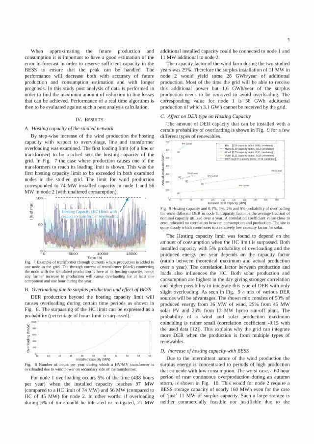
5

When approximating the future production and consumption it is important to have a good estimation of the error in forecast in order to reserve sufficient capacity in the BESS to ensure that the peak can be handled. The performance will decrease both with accuracy of future production and consumption estimation and with longer prognosis. In this study post analysis of data is performed in order to find the maximum amount of reduction in line losses that can be achieved. Performance of a real time algorithm is then to be evaluated against such a post analysis calculation.

IV. RESULTS

A. Hosting capacity of the studied network By step-wise increase of the wind production the hosting

capacity with respect to overvoltage, line and transformer overloading was examined. The first loading limit (of a line or transformer) to be reached sets the hosting capacity of the grid. In Fig. 7 the case where production causes one of the transformers to reach its loading limit is shown. This was the first hosting capacity limit to be exceeded in both examined nodes in the studied grid. The limit for wind production corresponded to 74 MW installed capacity in node 1 and 56 MW in node 2 (with unaltered consumption).

Fig. 7 Example of transformer through currents where production is added to one node in the grid. The through current of transformer (black) connecting the node with the simulated production is here at its hosting capacity, hence any further increase in production will cause overloading for at least one component and one hour during the year.

B. Overloading due to surplus production and effect of BESS DER production beyond the hosting capacity limit will

causes overloading during certain time periods as shown in Fig. 8. The surpassing of the HC limit can be expressed as a probability (percentage of hours limit is surpassed).

Fig. 8 Number of hours per year during which a HV/MV transformer is overloaded due to wind power on secondary side of the transformer.

For node 1 overloading occurs 5% of the time (438 hours per year) when the installed capacity reaches 97 MW (compared to a HC limit of 74 MW) and 56 MW (compared to HC of 45 MW) for node 2. In other words: if overloading during 5% of time could be tolerated or mitigated, 21 MW

additional installed capacity could be connected to node 1 and 11 MW additional to node 2.

The capacity factor of the wind farm during the two studied years was 29%. Therefore the surplus installation of 11 MW in node 2 would yield some 28 GWh/year of additional production. Most of the time the grid will be able to receive this additional power but 1.6 GWh/year of the surplus production needs to be removed to avoid overloading. The corresponding value for node 1 is 58 GWh additional production of which 3.1 GWh cannot be received by the grid.

C. Affect on DER type on Hosting Capacity The amount of DER capacity that can be installed with a

certain probability of overloading is shown in Fig. 9 for a few different types of renewables.

Fig. 9 Hosting capacity and 0.1%, 1%, 2% and 5% probability of overloading for some different DER in node 1. Capacity factor is the average fraction of nominal capacity utilized over a year. A correlation coefficient value close to zero indicated no correlation between consumption and production. The site is quite cloudy which contributes to a relatively low capacity factor for solar.

The Hosting capacity limit was found to depend on the amount of consumption when the HC limit is surpassed. Both installed capacity with 5% probability of overloading and the produced energy per year depends on the capacity factor (ration between theoretical maximum and actual production over a year). The correlation factor between production and loads also influences the HC. Both solar production and consumption are highest in the day giving stronger correlation and higher possibility to integrate this type of DER with only slight overloading. As seen in Fig. 9 a mix of various DER sources will be advantages. The shown mix consists of 50% of produced energy from 36 MW of wind, 25% from 45 MW solar PV and 25% from 13 MW hydro run-off plant. The probability of a wind and solar production maximum coinciding is rather small (correlation coefficient -0.15 with the used data [12]). This explains why the grid can integrate more DER when the production is from multiple types of renewables.

D. Increase of hosting capacity with BESS Due to the intermittent nature of the wind production the

surplus energy is concentrated to periods of high production that coincide with low consumption. The worst case, a 60 hour period of near continuous overproduction during an autumn storm, is shown in Fig. 10. This would for node 2 require a BESS storage capacity of nearly 160 MWh even for the case of ‘just’ 11 MW of surplus capacity. Such a large storage is neither commercially feasible nor justifiable due to the

0 5000 10000 150000

50

100

Time [h]

I [%

of Im

ax]

40 42 44 46 48 50 52 54 56 58 600

200

400

600

800

1000

Installed capacity (MW)

Ove

rload

ing

(hrs

/yr)

60 70 80 90 100 110 120 130 140 150 1600

100

200

300

400

500

600

700

Installed DER capacity [MW]

Ann

ual p

rodu

ctio

n[G

Wh]

HC

HC

5% Curtail

HC

5% Curtail

5% Curtail

5% Curtail

HC

HC

5% Curtail

Bio [1.00 capacity factor, 0.00 correlation]Hydro [0.39 capacity factor,- 0.12 correlation]Wind [0.29 capacity factor, 0.10 correlation]Solar [0.11 capacity factor, -0.23 correlation]DERmix[0.21 capacity factor, -0.14 correlation]

Hosting Capacity (HC) limit with respect to transformer overloading

6

infrequent use of the full storage capacity. Instead the avoided hours of overload and the non delivered energy to grid is studied as a function of the BESS storage capacity.

Fig. 10 Required storage capacity to fulfill the worst period of over production. Such a large storage is unfeasible both on economic grounds and due to the infrequent usage of the full installed capacity.

As shown in Fig. 11 a BESS of just one fortieth of the size required to avoid 100% of overloading can bring considerable benefits, eliminating as much as a third of the overloaded hours. Fig. 11. reveals that the effect on the performance index per MWh capacity decrease as the storage size increases over an amount of 4 MWh. This “diminishing returns per unit of storage capacity” is found for all nodes in the studied grid and also during studies of other grids (Fig. 12.).

Fig. 11 Avoided overloading with energy storage in node 2. Linear extrapolation reveals a best possible size after which a given unit capacity increase would give diminishing returns.

Fig. 12 The point of diminishing return has been found in other studies such as this 10 MVA 40/10 kV transformer in central Sweden.

E. Reduction of losses with BESS When the storage is controlled by a predictive algorithm

according to III. F. it is possible for the BESS to “shave” the maximum peak and thus reduce the maximum current during the overloading.

Fig. 13 gives comparison of the reduction in losses using such a method compared to the simpler method to charge as soon as overloading limit is surpassed. It should be remembered that the peak shaving method gives the theoretical maximum which will decrease with the error in estimation of future power flow. The BESS modeled in this

study [8] contains a power electronics converter that can be used to absorb and generate reactive power also during times when the storage is not being charged or discharged. This can be used to further reduce losses, as shown in Fig. 13.

Fig. 13 Annual losses from 2.4 km 234mm² FeAl 130 kV power line adjacent to energy storage at node 2. The greatest decrease on line losses arises from the BESS ability to continuously compensate for the reactive power from consumption (wind production is assume to be able to steer its reactive power production to zero). With 5% overloading the energy is being dispatched from battery between 3 to 5 % of the time (depending on storage size). This alteration of power flow will have an additional, but relatively small effect on the line losses. With peak shaving and discharge during minimum (according to III. F. ) the loss reduction is maximized, however the gain is most likely to small to motivate such a use of a BESS.

F. Influence of storage efficiency In the previous section an ideal storage has been assumed,

with only the storage size as limitation. Due to conversion losses in the BESS (that mainly come from the AC-DC and DC-AC conversion and the associated voltage level transformations) all energy taken from the grid cannot be returned. With losses in the BESS more energy is drawn from the grid in order to fill storage of a given capacity. This will actually decrease slightly the amount of overloaded hours compared to the case without conversion losses as seen in Fig. 14. However, conversion losses imply that less energy can be returned to the grid (Fig. 15).

Fig. 14 Conversion losses in the BESS will draw additional power from the grid. Therefore the same capacity of a BESS will avoid more overloading with lower efficiency. This is of cause energy that cannot be utilized (other than as heat) or returned to the grid as electricity.

Fig. 15 The BESS ability to decrease the amount of required production curtailment is influenced by its grid-to-grid round trip efficiency.

16600 16610 16620 16630 16640 16650 16661 16670 166800

20

40

60

80

100

120

140

160

Theo

retic

ally

requ

ired

ener

gy c

onte

nt [M

Wh]

Time [h]

0 1 2 3 4 5 6 7 8 9 100

10

20

30

40

50

60

70

80

90

100

StorageSize [MWh]

Avo

ided

ove

rload

ing

[%]

Avoided TR Overloading due to Energy Storage

Completely avoided overloadingPartialy avoided overloading

Limit after which increased storagesize provides diminishing returns

0 1 2 3 4 5 6 7 8 9 1048

48.5

49

49.5

50

50.5

51Losses in sub-transmission line closest to storage

Storage size [MWh]

Line

oss

es [M

Wh/

year

]

Continous VAR compensationQuick store/discharge with VAR comp.Peak shaving with VAR comp.

Max reactive power fromconsumption 8.5 MVAR

Mean reactive power fromconsumption 2.8 MVAR

0 1 2 3 4 5 6 7 8 9 100

10

20

30

40

50

StorageSize [MWh]

Avo

ided

ove

rload

ing

[%]

g gy g

Completely avoided overloading 100% efficiencyCompletely avoided overloading 90% efficiencyCompletely avoided overloading 80% efficiencyCompletely avoided overloading 70% efficiency

0 1 2 3 4 5 6 7 8 9 100

500

1000

1500

Storage size [MWh]

Cur

tailm

ent [

MW

h/ye

ar]

Energy not delivered to grid 100% efficiencyEnergy not delivered to grid 90% efficiencyEnergy not delivered to grid 80% efficiencyEnergy not delivered to grid 70% efficiency

Completely avoided overloadingPartialy avoided overloading

7

G. Influence of charge and discharge power In section IV. C. the converter sizes is chosen so that the

time to charge and discharge the storage from empty to full capacity is 1 hour. For handling overloading the priority is instead to charge quickly. The effect of varying charging power is shown in Fig. 16. The storage will frequently be hindered from reaching its full capacity when charging time is increased from one hour (left) to ten hours (right)..

Fig. 16 Effect of charging power in node 2. In the left figure the storage can be completely filled within an hour. In the right figure the time to load the storage is instead 10 hours. This will prolong the life-time of the battery but the charging power - rather than the capacity - now limits the amount of energy that can be stored. The reduced charging power means that the BESS will reach its maximum capacity more seldom, before discharge starts.

As the charging capacity poses an increasing limitation to the loading of the storage, the number of hours that overloading will be avoided decreases. This is shown in Fig. 17. Likewise the amount of energy that must be curtailed (cannot be delivered to grid) increases as the charging power, rather then the storage capacity, becomes limiting (Fig. 18).

Fig. 17 Decrease in hours where overloading can be avoided for smaller power rating of the BESS charger

Fig. 18 Decrease in avoided curtailment with different charging power

In Fig. 19 and the discharge time is varied from 1 to 10 hours. Because the average time between overloading peaks (68 hours) is considerably longer than the average duration of the overloading (4.3 hours) the discharge power of the BESS has less impact then the charging power but is still significant for storage size around the point of diminishing returns. The increase in non-delivered energy is only 1.3-2% in this case and therefore not shown in a figure.

Fig. 19 Decrease in hours where overloading can be avoided for smaller power rating of BESS discharge.

V. DISCUSSION

A. Modeling of battery storage Battery energy storage systems are highly non-linear and

the chemical reactions at the anode and cathode are not 100% reversible. The ions require a certain time to travel through the electrolyte and the battery cells need to reach equilibrium between storage cycles to function optimally.

A large BESS consist of thousands of individual battery packs and the power electronics and battery management system is of vital importance for the overall behavior of the BESS. Refinement of the simple energy storage model used here could include detailed state-of-charge estimation and modeling of the varying losses depending on different charging/discharge power levels. Such data is often kept by the supplier and not openly available. This is specifically the case for a relatively new and immature product as the large scale Li-ion BESS systems being piloted today.

B. Dimensioning of energy storage The aim of this study was to develop methods to dimension

the capacity and power ratings of a BESS storage system using the hosting capacity approach. In order for the developed methodology to be easily applicable to utilities concern was given to limit the required input data to such information that is readily available to a DSO. This consists of hourly data for consumption and production in the point of grid connection (such metering infrastructure is today common place in Sweden and being developed or planned in many other countries) as well as basic line and transformer data required for load flow calculation. The time correlated load and production data need to be sufficiently long (e.g. a full year with hourly data) in order to be able to calculate the probabilities also for the unlikely but dimensioning event.

For a DSO it is desirable to be able to see the BESS largely as a “black-box” characterized by its capacity and power ratings. As has been shown in this paper the influence of power rating of the BESS will greatly affect the performance of a BESS and must be selected carefully. The effect of the efficiency is smaller but will never the less have an influence on the results around the point of diminishing returns. Today there are suppliers of MWh capacity BESS systems guaranteeing up to 90% grid-to-grid efficiency [17]. However this efficiency is under certain conditions and will decrease for shorter charging or discharging periods. It is therefore

11000 12000 13000 140000

2

4

6

8

10

Time [h]

11000 12000 13000 140000

2

4

6

8

10

Time [h]

Ene

rgy

cont

ent [

MW

h]

0 1 2 3 4 5 6 7 8 9 100

10

20

30

40

50

StorageSize [MWh]

Avo

ided

ove

rload

ing

[%]

g gy g

Completely avoided overloading 1h chargingCompletely avoided overloading 4h chargingCompletely avoided overloading 7h chargingCompletely avoided overloading 10h charging

0 1 2 3 4 5 6 7 8 9 100

500

1000

1500

Storage size [MWh]

Cur

tailm

ent [

MW

h/ye

ar]

Decrease of Curtailment with Energy Storage

Energy not delivered to grid 1h chargingEnergy not delivered to grid 4h chargingEnergy not delivered to grid 7h chargingEnergy not delivered to grid 10h charging

0 1 2 3 4 5 6 7 8 9 100

5

10

15

20

25

30

35

40

45

50

StorageSize [MWh]

Avo

ided

ove

rload

ing

[%]

Completely avoided overloading 1h dischargeCompletely avoided overloading 4h dischargeCompletely avoided overloading 7h dischargeCompletely avoided overloading 10h discharge

8

important to have complete picture of varying efficiency during different operating scenarios when evaluating the BESS performance.

In this paper the fast charging was found to be more important than fast discharge. Generally the length of the time during which the storage is to be filled compared to the available time period to empty it will influence the optimal power ratings. For other applications of a BESS like load shedding the relation between for charging and discharge power may be reversed.

VI. CONCLUSIONS

A. General The quantification of the hosting capacity for the various

nodes of a grid is an important tool to scan a grid for suitable DER locations and aim investment efforts towards the true bottle necks of the grid. This paper shows that accurate dimensioning of a BESS is possible using the hosting capacity method and readily available data from utilities revenue metering systems. The methodology can be extended to other applications such as load shedding or other storage techniques like molten salt (for heat from solar reflectors), pumped hydro (topology permitting) or compressed air (with gas turbine).

As found in this study, the capacity per unit benefit of the BESS system decreases with increasing storage size. This phenomenon we call “diminishing returns per unit of storage capacity”. Therefore it is possible to talk about a technically optimum size for a given grid and DER production characteristics. This technical optimum may differ from the economical optimal dimensioning of BESS storage capacity and converter power rating. The economy of the BESS will be influenced by the selected application, market price for the ancillary services provided by the storage and regulatory framework, including ability to add investment to tariff cost base of the utility. However any economic evaluation needs to consider the physical restrictions of the storage technology.

B. BESS application for avoiding overload Different applications require different control algorithms

that are more or less suitable for real-time application. The results in this paper show that the energy storage application for avoiding overloading is a partial solution that for practical reasons needs to be combined with other means such as curtailment.

VII. REFERENCES [1] L. Ferris and D. Infield, Renewable Energy in Power Systems,

Chichester: Wiley, 2008. [2] M. Delfanti, M. Merlo, V. Olivieri and G. M, "Power flows in the

Italian distribution electric system with dispersed generation," in International Conference on, Prague, 2009.

[3] J. Wong, R. Baroutis, R. Chadha, M. Iravani, M. Graovac and X. Wang, "A methodology for evaluation of permissible depth of penetration of distributed generation in urban distribution systems," in IEEE Power Engineering Society General Meeting, Pittsburgh, 2008.

[4] D. Rastler, Electricity Energy Storage Technology Options: A White Paper on Applications, Costs, and Benefits, U. S. A., CA: Electrical Power Research Institute, 2010.

[5] J. Eyer and G. Corey, "Energy Storage for the Electricity Grid:

Benefits and Market Potential Assessment Guide, A Study for the DOE Energy Storage Systems Program," Sandia National Laboratories, USA, California, 2010.

[6] V. Giordano, F. Gangale, G. Fulli and S. J. Manuel, “Smart Grid Projects in Europe - Lessons Learned and Current Developments,” Publications Office of the European Union, 2011.

[7] C. Vartanian and N. Bentley, "A123 systems' advanced battery energy storage for renewable integration," in IEEE/PES Power Systems Conference and Exposition (PSCE), Phoenix, 2011.

[8] J. Berst, "Smart Grid News," Global Smart Energy, 7 09 2011. [Online]. Available: http://www.smartgridnews.com/artman/publish /Technologies_Storage/Lithium-ion-for-grid-scale-storage-3981.html. [Accessed 29 03 2012].

[9] M. Bollen and F. Hassan, Integration of Distributed Generation in the Power System, U. S. A.: John Wiley & Sons, Inc., 2011.

[10] European Regulators Group for Electricity and Gas, "Position paper on smart grids," ERGEG, Brussels, 2010.

[11] The European Network of Transmission System Operators, "European Electricity Grid Initiative Roadmap and Implementation plan," ENTSO-E, Brussels, 2010.

[12] N. Etherden and M. H. J. Bollen, "Increasing the Hosting Capacity of Distribution Networks by Curailment of Renewable Energy Resources," in 2011 IEEE Power Tech, Norge, Trondheim, 2011.

[13] M. Bollen and N. Etherden, "Overload and overvoltage in low-voltage and medium-voltage networks due to renewable energy – some illustrative case studies," in IEEE PES ISGT Conference, Manchester, 2011.

[14] N. Etherden, M. Gudmundsson, M. Häger and H. Stomberg, "Experiance from Construction of a Smart Grid Research, Development and Demonstration platform," in Proceedings of CIRED 21st International Conference on Electricity Distribution, Frankfurt, 2011.

[15] Y. Hida, R. Yokoyama, J. Shimizukawa, K. Iba, K. Tanaka and T. Seki, "Load following operation of NAS battery by setting statistic margins to avoid risks," in Power and Energy Society General Meeting, Minneapolis, 2010.

[16] N. Ding, Y. Besanger, F. Wurtz, G. Antoine and P. Deschamps, "Time series method for short-term load forecasting using smart metering in distribution systems," in PowerTech, 2011 IEEE, Trondheim, 2011.

[17] Kema, "Summary of AltairNano Validation Testing," The AES Corporation, 2008.

VIII. BIOGRAPHIES

Nicholas Etherden works at STRI AB as a specialict consultant in power utility automation and is an Industrial postgraduate student at Electric Power Engineering department, Lulea University of Technology, Sweden. He has an MSc in Engineering Physics from Uppsala University in Sweden, 2001. He has several years experience as relay application engineer, project manager and product marketing manager at ABB. Since 2008 he is responsible for the STRI IEC 61850 Independent Interoperability

Laboratory and a member of IEC TC 57 working group 10 and UCA/IEC 61850 User group testing subcommittee.

Math Bollen (M'93, SM'98, F'05) received the M.Sc. and Ph.D. degrees from Eindhoven University of Technology, Eindhoven, The Netherlands, in 1985 and 1989, respectively. Currently, he is professor in electric power engineering at Luleå University of Technology, Skellefteå, Sweden, senior specialist at STRI AB, Ludvika, Sweden and technical expect at the Energy Markets Inspectorate, Eskilstuna, Sweden. He has also been a lecturer at the University of Manchester Institute of Science and Technology

(UMIST), Manchester, U.K., and professor in electric power systems at Chalmers University of Technology, Gothenburg, Sweden. He has published a number of fundamental papers on voltage dip analysis and power quality, as well as books on “Integration of Distributed Generation in the Power System” and “The Smart Grid - adapting the Power System to New Challenges”.

Paper IV

Effect of Large Scale Energy Storage on CO2 Emissions in Scandinavian Peninsular

N. Etherden, M. Bollen

Approved paper to the Tenth Nordic Conference Electricity on Distribution System Management and Development, Esbo, September 2012

1

EFFECT OF LARGE SCALE ENERGY STORAGE ON CO2 EMISSIONS IN THE SCANDINAVIAN PENINSULA

Nicholas Etherden, Math H.J. Bollen

STRI AB and Luleå University of Technology Contact: Nicholas.etherden@stri.se

ABSTRACT This paper investigates some aspects of greenhouse gas emissions related to large scale use of energy storage. Energy storage enables production and consumption to be decoupled in time so that production mix, network loading and energy prices will be different at the time of loading and discharge. The storage consumes electricity produced with one carbon intensity and releases it when production has another carbon intensity. Electricity in the Scandinavian Peninsula is mainly from low carbon sources. The marginal and mean greenhouse emissions vary from hour to hour and are shown to be strongly dependent on the degree of net import of electricity during each hour. In Sweden emissions from consumed energy are largest during the night when consumption is lowest. This is the opposite case to most other European countries. Therefore several studied energy storage applications would fail to produce the greenhouse gas reduction that would occur in other countries. INTRODUCTION Figure 1 shows the variation in carbon intensity for electricity in Sweden 2010.

Figure 1 Carbon intensity of Swedish electricity production 2010. (Bottom line: daily average, green area: extent of daily variation). During winter import of electricity was greater then the export. Based on the average emissions from imported electricity the carbon intensity of all consumed electricity is calculated (top line: daily average, red area: daily variation).

Time [hour of year 2010]

Carb

on in

tens

ity [g

CO2/

kWh]

2

In a Vinnova project entitled “Smart Grid Energy Storage” led by High Voltage Valley the effect of large scale energy storage is studied in several PhD projects at Luleå University of Technology, Stockholm Royal Institute of Technology and Uppsala University. Part of the work concerns studies of how energy storage can affect the hosting capacity of Distributed Energy Resources on existing regional grids [4]. As a complement to regulatory and economical aspects of the storage this work focuses on the influence on greenhouse gas emissions from the use of energy storage.

In order to reduce greenhouse gas emissions and achieve a more sustainable energy sector an increasing proportion of the electricity needs to be produced by renewable energy resources [1] [2] [3]. The electricity production from renewables will increase as the wind blows and the sun shines and the network needs to handle this intermittency. The basic principle of power-system operation is that production and consumption are always in balance. To avoid reducing output from renewables at times of over production, consumption must be managed to match production (demand-response). Alternatively energy storage can be used to store the surplus and release this during times of shortage. By combining demand-response, curtailment of overproduction of renewables and energy storage, high penetration of renewables. It is possible to meet even the most ambitious environmental targets.

Electricity generation in the Scandinavian Peninsula (Norway and Sweden) is dominated by hydro and nuclear power with low greenhouse gas emissions. Imports to this region will therefore likely increase the average CO2 emission of the total electricity consumed. This can be measured as the carbon intensity in gCO2 equivalents per kWh consumed energy. The variation in carbon intensity for electricity produced (green) and consumed (red) in Sweden during 2010, is shown in Figure 1. As seen in Figure 1 the import of electricity has a considerable influence on the carbon intensity of the consumed electricity in Sweden. This needs to be considered if the aim of renewables is to help decarbonise the energy sector. As energy is moved in time it will be stored when production has one composition of sources and released when production has another. Carbon intensity will therefore also vary between stored and released energy. However inevitable conversion losses (ranging from 10 to 30 % for battery storage) of the stored energy will increase the total amount of energy that needs to be produced. Greenhouse gas emissions from Swedish electricity sources The climate impact from any one energy source is often a matter of lengthy debate. When the green house gas emissions are dominated by fossil fuel use the results of different life-cycle analyses are fairly similar but will be affected by assumptions of how it is excavated, transported and the efficiency in the electricity conversion and transfer. When the greenhouse gas contribution is indirect (i.e. not primarily from the fuel itself) there is considerable variation in the results of the life-cycle analyses. Estimates vary depending on the type of technology used (e.g. run-off or large dam installations for hydro) and the completeness of the life-cycle analysis performed (extent to which mining, plant construction, transport and decommissioning of a plant etc are included). Another factor that can affect the results is alternative land-use (clearing of forest for biofuel crops or hydro reservoir). In determining

3

the carbon intensity of an energy source the production of different greenhouse gas needs to be analyzed and then converted to CO2 equivalents. A multitude of promotion organisations exist for most energy resources with interest in showing their resource more favourable. For comparison the data should be collected in a neutral, scientific way with a similar life-cycle approach. Table 1 is based on data from [5] with the exception of values for nuclear power that were deemed as low compared to other studies and values from [6] used instead.

Table 1 Carbon intensity and share of total electricity production 2010 Electricity Source Wind Hydro Nuclear Gas/Diesel CHP Carbon intensity 10.4 gCO2/kWh 5.3 gCO2/kWh 6 gCO2/kWh 450 gCO2/kWh 187 gCO2/kWh Share of production 2.5 % 47.7 % 39.5 % 0,1 % 8.9 % Source [5] [5] [6] [5] [7] and [5]

The emissions from Combined Heat and Power (CHP) plants are particularly difficult to determine as both electricity and distributed heating is produced. CHP plants constituted 9 % of the total electricity production in Sweden during 2010. Part of the emissions need to be ascribed to the heat production and part to electricity production. In a CHP plant both electricity and heat are normally produced at a lower efficiency than a plant optimised for one or the other production. Therefore the electricity can not be considered a pure bi-product of the heat (or vice versa). The allocation of emissions to one or the other energy carrier becomes complex if not arbitrary.

The approach of this paper is to consider the produced electricity from CHP plant as coming from an equivalent plant optimised for electricity only production. The fuel of the CHP plant was taken as the average mix used in Swedish district heating plants. According to [7] this mix for both industrial and domestic heating consists to two-thirds from bio fuels, nearly one-third from natural gas and one-twentieth from waste combustion residues. With the values of Table 1 this would be equivalent to 187 gC02/kWh from a plant designed for pure electricity production. (The value is comparable to using 13.5 gCO2/kWh for electricity from bio fuel fired CHP plant and 600 gCO2/kWh from coal fired CHP plant given in [5].)

Based on the hourly production mix for 2010 [8] the average emission from Swedish electricity production was found to be 21 gCO2/kWh. During the summer months, with low consumption, 99 % of electricity was produced by hydro and nuclear, and greenhouse gas emissions are as low as 5.8 gCO2/kWh. At times when electricity consumption was 50 % above its mean value, emissions soared to 43 gCO2/kWh and the fraction of electricity from hydro and nuclear decreased to 79 %.

Greenhouse gas emissions from Imports During 2010 electricity imports were greater than exports for 5407 hours out of 8760 and Sweden was a net importer of electricity (the same was the case 2009 but not 2011). The imports occurred mainly during the winter and autumn months as can be seen in Figure 2.

4

Figure 2 Net import (positive) and export (negative) of electricity 2010 as percent of the domestic consumption in Sweden.

Nord Pool Spot [9] provides data on imports and exports to Norway, Finland, Denmark, Germany and Poland. Imports were on average just over one percent of the total consumption. They constituted more than 5% of the consumption 15% of the time. On rare occasions the imported electricity corresponded to as much as 20-30 % of consumption. Even if the amount of imported electricity is relatively small it makes a considerable contribution to the average greenhouse gas emissions from the consumed electricity in Sweden. This is because all neighbouring countries, except Norway, have considerably greater carbon intensity from their electricity production than Sweden, as seen in Table 2. Note though that the carbon intensity of imported electricity is taken as annual average from [10]. A deeper analysis of the hourly production mix is required to reveal if imports take place when Denmark and Northern Germany have overproduction of wind and other low carbon sources.

Table 2 Average carbon intensity from electricity and heat according to [10] Electricity Source Norway Finland Denmark Germany Poland Carbon intensity 17 gCO2/kWh 205 gCO2/kWh 303 gCO2/kWh 430 gCO2/kWh 640 gCO2/kWh Share of imports 18 % 29 % 35 % 15 % 3.7 %

According to [10] the Swedish emissions were on average 43 gCO2/kWh 2009. As this value is for both electricity and heat production the results are in line with those derived in this work. Average and marginal emissions from energy production In determining the carbon intensity of energy production (measured as gCO2 per kWh) the choice is between using an average value based on the production mix at a given time or using the value of the last (marginal) production unit dispatched. The average CO2 emissions are possible to calculate for many countries and Transmission System Operator (TSO) areas, based on statistics of the hour-by-hour generation mix. Such values are available for Sweden at [8] and provide the total consumption and electric production from wind, hydro, nuclear gas/diesel, and CHP. Solar and unspecified production is also given but account only for a

5

fraction of a percent of the total production. To get the mean value of consumed electricity also use of imported electricity is to be considered.

In theory emission from the marginal source could be obtained according to Figure 3. Here a surplus of low carbon renewables would be stored and later dispatched to avoid imported production from fossil giving a gain of up to 600 gCO2/kWh.

Figure 3 Principle of marginal emissions where storage is filled in hours with surplus of renewables and released during hours of shortage.

While the approach of Figure 3 may be justifiable for a micro grid the approach is questionable for the production of an entire country like Sweden. Figure 4 shows the relation between carbon intensity and prices. Although a weak general trend may be distinguishable, a closer look at the vast majority of the hours with prices around the mean price shows only weak correlation between emissions and price.

Figure 4 Relationship between carbon intensity and spot market price for Swedish electricity production 2010. The insert shows the 97% of the hours where the spot market price was under 1 SEK/kWh (mean was 0.54 SEK/kWh).

Including imports the relationship between carbon intensity and cost is all but lost. From Figure 5 it appears that the market does not give preference to local low carbon production as long as transfer capacity is sufficient. Note though that the carbon intensity of imported electricity is taken as annual average from [10].

6

Figure 5 Relationship between carbon intensity and spot market price for Swedish electricity consumption 2010. The hours of high carbon intensity come from contribution from imports. Here the price shows little or no correlation to the carbon intensity of the production.

Another way to derive a marginal price would be to look at the source of the electricity used to bid on the day ahead spot market or balancing market. The marginal sources can then be taken as the last accepted bid(s). However, the marginal bid may well be less carbon intense than the average production (for the regulatory market in Sweden almost all bids are coming from hydro plants). As it is an economic market no certainty is provided that taxation and price mechanisms are today sufficient to ensure that low carbon energy sources are utilised first. This approach was also dismissed because there was even less correlation between emissions and regulatory price than between emissions and spot price. EFFECT ON CO2 EMISSIONS FROM LARGE-SCALE ENERGY STORAGE

An overview of some possible applications for energy storage in the electricity network is given in Figure 6. Here we consider battery storage with a few cycles per day in order to get acceptable life-time and sufficient revenue from cycling.

Figure 6 Characteristic time scale of energy storage applications.

A large scale energy storage system is today a significant investment. If the payback comes from cycling the storage it will be unjustifiable to store energy during long periods. Also application on the far left of Figure 6 are often uneconomical due to the high number of cycles as e.g. Li-Ion battery today have lifetime expectancy (defined as 20 % drop in capacity) of only a few thousand cycles. The applications of most storage technologies will be a balance between many cycles of maximizing profit and minimising the number of cycles to give an acceptable storage life-time.

0 20 40 60 80 100 1200

2

4

6

8

10

12

14

Carbon intensity [gCO2/kWh]

Spot

pric

e [S

EK/kW

h]

7

Daily variation in carbon intensity In order to study the impact of energy storage when acting as intermediate storage over one or two days, hourly carbon intensity fluctuations is of greatest importance and is shown in Figure 7. The daily carbon intensity variation is reversed to both the consumption and spot market price shown in Figure 8. This study found that imports occur, not at times of high energy need (the day-time peak in Sweden that follows the spot market price shown in Figure 8), but instead during the night at times of “cheap” electricity from over-production on the continent. These night hours are also when the transfer capacity is most highly used.

Figure 7 Daily average of carbon intensity 2010

Figure 8 Average daily variations in spot market price 2010

It can be concluded that carbon intensity follows the amount of imported energy rather than the consumption. (This statement is also true when Sweden is a net exporter of electricity as shown by the lower curve without imports in Figure 7.)

The results of Figure 7 are explained by Figure 9 and Figure 10. The carbon intensity from the low emission sources follows the consumption pattern (Figure 9). These sources stand for 90 % of all electricity produced in Sweden during 2010. They peak when consumption peaks and thus carbon intensity does not grow with consumption.

Figure 9 Hourly distribution of electrical power from low carbon electricity sources. The wind production (multiplied by 10 in the figure) shows a small variation with increased wind during the night.

Figure 10 Hourly distribution of imports and carbon intense electricity sources. Imports are largest during the night. CHP and reserve gas/diesel power (multiplied by 100 in the figure) follow the daily load profile.

0 5 10 15 20 2515

20

25

30

35

40

45

50

Hour of the day

CO

2 [g

/kW

h]

g y

Swedish productionIncluding imports

0 5 10 15 20 250

0.05

0.1

0.15

0.2

0.25

0.3

0.35

0.4

0.45

0.5

hour of the day

pric

e [S

EK

/kW

h]

5 10 15 200

2

4

6

8

10

12

14

16

18

20

Hour of the day

Powe

r [G

Wh

nucl

ear h

ydro

, 100

MW

h wi

nd]

Total productionNuclear powerHydro + Nuclear10*Wind

0 5 10 15 20 250.8

1

1.2

1.4

1.6

1.8

2

2.2

2.4

2.6y p p y

Hour of the day

Pow

er [G

Wh

CH

P &

Impo

rted,

10

MW

h G

as/D

iese

l]

CHPImported electricity100*Gas/Diesel

8

Although the low carbon sources dominate the total amount of produced energy, the variation in carbon intensity is governed by imports and, to lesser degree, the carbon intense domestic production shown in Figure 10. During early morning hours, imports average over the year as much as the electricity production from CHP plant. While the production of gas and diesel used as reserve power follows the peak load, their contribution has little or no impact on the average carbon emission levels, except for a few hours when they constitute 2% of the total production. (Production for gas and diesel is multiplied by 100 in Figure 10). EXAMPLES OF GREENHOUSE GAS EMISSION IMPACT FROM LARGE-SCALE ENERGY STORAGE Ride-through carbon intense periods From Figure 1 it can be derived that the gain of storage from a daily cycle would be between 60 and 80 gCO2/kWh in winter but only about 10 gCO2/kWh in summer. Over the year the average is 15 gCO2 gain per day and kWh storage capacity (Figure 7). The annual reduction of greenhouse gas emissions would be less than 6 kg of carbon dioxide equivalents per kWh storage capacity and year. A measure of the value of this amount of greenhouse gas emissions is the costs for climate compensation of as little as 0.10 SEK/kg found on some commercial sites.

This is very far from the theoretical gain with gas/diesel reserve power or imports as marginal electricity source that would result in gains of up to 600 gCO2/kWh according to the section Average and marginal emissions from energy production. Such a gain would result in avoided emissions of 0.2 tons of CO2 per year and kWh storage capacity.

Conversion losses will also decrease the gain from the use of the storage. For a Li-Ion system they can be as low as 10 % conversion losses (grid-to-grid) which would be equivalent to 2 gCO2/kWh emissions if taken at the average carbon intensity.

The storage would be emptied at night when consumption is low and energy cheap and filled during peak loading in the day with high energy costs making the application unattractive economically. The losses on spot market price could be compensated if the user of the storage would be entitled the sell the gain as green certificates. The loss of 0.15 SEK/kWh from the average price difference between night and day in Figure 8 would be compensated by the value of green certificates that averaged 0.29 SEK per kWh during 2009-2010. Still there is no profitability. The higher differences on the balancing market could possibly result in some profitability. Spot market trading and peak load support The use of energy storage in Sweden for energy trading will imply storing at night and discharging during the day, which will have a negative effect on greenhouse gas emissions. The average daily spot market variation in Sweden 2009-2010 was 0.15 SEK/kWh (Figure 8). Compare this to the cost of 1 kWh of battery storage, which is today around 10 000-30 000 SEK/kWh. Even with best estimates for future price, in the range of 350 US$/kWh [11],

9

there is no profitability in such an application even if the price differences during the day would increase several fold on the spot market.

The first grid-scale energy storage in Sweden is a 75 kWh unit in Falköping [12]. It charges during 3 hours at night and discharges during an hour of peak load in the afternoon. The price and consumption were found to follow each other. Therefore the use of energy storage for peak load support will have a negative impact on greenhouse emissions. In 2010 this application would have resulted in a net increase in greenhouse gas emissions of 8 kg/kWh storage capacity or 0.6 tons for the entire storage during 2010 (assuming 10 % conversion losses in the storage). Reduction of imports with storage As seen from Figure 5 there is little or no correlation between electricity price and carbon intensity. The price is related to the consumption. It therefore follows that consumption does not relate to carbon intensity. As this example shows it is therefore better use the storage for greenhouse gas emissions only under specific circumstances, the rest of the time the storage can be used for other applications. Such a specific circumstance could be to store renewables that would otherwise not be possible to consume or export and use the energy to avoid imports. To avoid storing energy for long periods (blocking other use of the system) the storage would be utilized for greenhouse gas reduction only during days of both export and import. This happens mainly in the spring and autumn (see Figure 1). Calculating the emissions savings over 45 possible storage cycles over 33 days during 2010, the CO2 equivalent emissions saving would correspond to 7 kg per year and kWh storage capacity.

Further investigation is required into the generation mix of imported electricity to see if import is due to over production of low carbon wind energy in Denmark and Northern Germany. If the energy used to fill the storage could be instead exported to the continent and replace fossil fuels there, the reduction saving could also be much greater. COMPARISON WITH GREAT BRITAIN The average daily profile of the carbon intensity of consumed electricity in Figure 7 is in stark contrast to that seen in continental European and Great Britain. In Great Britain the use of storage has been proposed to be used as “ride-through of time of carbon intense production” [13]. Here the consumption peak corresponds to times production with high carbon intensity. Therefore use of storage to decrease peak load would decrease the overall green-house gas emissions even accounting for the affect of losses (10-15% of stored energy), which, as the previous examples show does not apply in Sweden.

From Figure 11 it can be seen that the saving from ride-through of carbon intense production in Great Britain would be 72 gCO2/kWh storage capacity per working day. This compares to a gain of about 5 gCO2/kWh in this study (lower line in Figure 7).

10

Figure 11 Carbon intensity of UK Electrical network [13].

CONCLUSIONS When estimating greenhouse gas emissions from energy production many factors need to be taken into account. Many of these are difficult to estimate even though they have a significant effect on the results. This study shows that the use of energy storage in Sweden is likely to have a negative impact on greenhouse gas emissions. This is because storage takes place with low consumption and high carbon intensity (due to imports) with the stored energy released to the electricity network during high consumption (and only domestic production and therefore lower gCO2/kWh).

For a small community or region like Gotland or Bornholm seeking to achieve carbon neutrality with self-production and local storage local accounting of Carbon dioxide emissions is valid only if transfer of energy out of the area is restricted. But otherwise, local accounting of emission makes less sense tas climate change is global and knows no borders. If instead transfer capacity between countries would be increased and balancing regions enlarged to cover a significant part of Europe this could enable for more efficient greenhouse gas reduction from storage.

The true environmental benefit of the storage lies not in its ability to store low carbon production per se, but in its ability to potentially increase the possible proportion of renewable generation. In the future, storage may contribute to lowering the cost of connecting these resources by managing the increased variability of generation, which is the main field of our research [14] [15] [4]. ACKNOWLEDGMENTS: This work is part of research project titled “Smart Grid Energy Storage” at HVV (www.highvoltagevalley.se) and financed by the Swedish Governmental Agency for Innovation Systems.

11

REFERENCES

[1] IPCC, “IPCC Fourth Assessment Report: Climate Change 2007,” IPPC, Geneva, Switzerland, 2007.

[2] Working Group III of the Intergovernmental Panel on Climate Change, “Special Report on Renewable Energy Sources and Climate Change Mitigation,” IPCC, Cambridge, 2011.

[3] European Commision, “Energy Roadmap 2050,” Publications Office of the European Union, Luxembourg, 2012.

[4] N. Etherden, Licentiate of Engineering Thesis: Increasing the Hosting Capacity of Distributed Energy Resources using Storage and Communication, Luleå : Luleå University of Technology, Department of Engineering Science and Mathematics, Division of Energy Engineering, 2012.

[5] Vattenfall AB, “Livscykelanalys Vattenfalls el i Sverige,” Vattenfall Bussiness Service Nordic AB, Stockholm, 2005.

[6] United Kingdom Parlimentary Office of Science and Technology, “Postnote number 268: CARBON FOOTPRINT OF ELECTRICITY GENERATION,” Parliamentary Office of Science and Technology, London, October 2006 .

[7] Svensk Energi, “Statistik om den svenska elförsörjningen,” Svensk Energi, 17 01 2012. [Online]. Available: http://www.svenskenergi.se/sv/Om-el/Statistik/. [Accessed 17 01 2012].

[8] Svenska Kraftnät, “Elstatistik för hela Sverige,” Svenska Kraftnät, 17 01 2012. [Online]. Available: http://www.svk.se/Energimarknaden/El/Statistik/Elstatistik-for-hela-Sverige/. [Accessed 17 01 2012].

[9] Nord Pool Spot , “Data download page,” Nord Pool Spot , 10 01 2012. [Online]. Available: http://www.nordpoolspot.com/Market-data1/Downloads/Historical-Data-Download1/Data-Download-Page/. [Accessed 10 01 2012].

[10] International Energy Agency, “I E A S T A T I S T I C S: CO2 EMISSIONS FROM FUEL COMBUSTION H I G H L I G H T S,” International Energy Agency, Paris, 2011 Edition.

[11] H. K. Trabish, “Green Tech Media,” 7 October 2010. [Online]. Available: http://www.greentechmedia.com/articles/read/energy-storage-for-the-grid-better-than-the-holy-grail/. [Accessed 12 04 2012].

[12] J. Berst, “Smar GridNews.com,” 7 Septemeber 2011. [Online]. Available: http://www.smartgridnews.com/artman/publish/Technologies_Storage/Lithium-ion-for-grid-scale-storage-3981.html. [Accessed 7 May 2012].

[13] B. J. Williamson, M. A. Redfern, R. K. Aggarwal, J. Allinson, C. Harris, P. Bowley and R. Hotchkiss, “Project Edison: SMART-DC,” in 2nd IEEE PES International Conference and Exhibition on Innovative Smart Grid Technologies (ISGT Europe), Manchester, 2011.

[14] M. Bollen and N. Etherden, “Overload and overvoltage in low-voltage and medium-voltage networks due to renewable energy – some illustrative case studies,” in IEEE/PES Innovative Smart Grid Technologies, Manchester, 2011.

[15] N. Etherden and M. H. J. Bollen, “Increasing the Hosting Capacity of Distribution Networks by Curailment of Renewable Energy Resources,” in 2011 IEEE Power Tech, Norge, Trondheim, 2011.