
ISR REU Program ‘06 - University Of Maryland · and in Microsoft Excel we started to create our...
33
ISR develops, applies and teaches advanced methodologies of design and analysis to solve complex, hierarchical, heterogeneous and dynamic problems of engineering technology and systems for industry and government. ISR is a permanent institute of the University of Maryland, within the Glenn L. Martin Institute of Technol- ogy/A. James Clark School of Engineering. It is a National Science Foundation Engineering Research Center. Web site http://www.isr.umd.edu IR INSTITUTE FOR SYSTEMS RESEARCH UNDERGRADUATE REPORT Systems Engineering: Quick Dispensing Clinic and Schroeder Industries by Kristen Gaska and Kirsten Gheen Advisor: UG 2006-4
Transcript of ISR REU Program ‘06 - University Of Maryland · and in Microsoft Excel we started to create our...

ISR develops, applies and teaches advanced methodologies of design and analysis to solve complex, hierarchical,heterogeneous and dynamic problems of engineering technology and systems for industry and government.
ISR is a permanent institute of the University of Maryland, within the Glenn L. Martin Institute of Technol-ogy/A. James Clark School of Engineering. It is a National Science Foundation Engineering Research Center.
Web site http://www.isr.umd.edu
I RINSTITUTE FOR SYSTEMS RESEARCH
UNDERGRADUATE REPORT
Systems Engineering: Quick Dispensing Clinic and Schroeder Industries
by Kristen Gaska and Kirsten GheenAdvisor:
UG 2006-4

ISR REU Program ‘06
Systems Engineering: Quick Dispensing Clinic and Schroeder Industries
Kristen Gaska and Kirsten Gheen
Advisor: Dr. Jeffrey Herrmann
August 11, 2006
University of Maryland: ISR
1
Table of Contents
Table of Contents ................................................................................................................ 1 Introduction: .................................................................................................................... 2 Brooke Grove .................................................................................................................. 3
Background: ................................................................................................................ 3 Procedure:.................................................................................................................... 4 Simulation Set-Up:...................................................................................................... 7 Analysis:...................................................................................................................... 8 Conclusion:................................................................................................................ 10
Schroeder Industries...................................................................................................... 11 Background: .............................................................................................................. 11 Process:...................................................................................................................... 11 Assumptions:............................................................................................................. 13 Simulation Set-Up:.................................................................................................... 13 Future Progress:......................................................................................................... 19
Final Reflections: .......................................................................................................... 20 Appendix A ....................................................................................................................... 21 Appendix B ....................................................................................................................... 26

University of Maryland: ISR
2
Introduction:
During the course of our ten-week program, we have been working with Dr.
Jeffrey Herrmann on projects involving computer simulations. We have had two projects
dealing with applied industrial engineering theories, Brooke Grove Clinic and Schroeder
Industries.
Our first assignment was to read and understand the software Dr. Hermann and
his team has created over the past five years. The Clinic Generator Software was created
from results of numerous simulated vaccinations to help prepare local authorities in case
of bio-terrorism or life-threatening infectious diseases. We used and tested the software
after reading the user’s guide to make sure that there were no errors before the release of
the new version. By testing the new version, we were able to help resolve problems such
as the ability to open specific files on different computer systems. Figure 1 is the first
screen when the software is opened. This is where the user begins to input their
information. Figure 2 is a sample screen of the results the software will produce after the
appropriate information is entered. Simultaneously, we were given the assignment of
learning the simulation software program, Arena, so that we could use it for future
projects.
Figure 1 Figure 2

University of Maryland: ISR
3
Brooke Grove Planning for biological terrorist attacks has been a focus for state and local public
health agencies since the terrorist attacks of September 11, 2001. Public health officials
must be prepared and capable to provide quick dispensing of medicine to all persons
affected by a biological terrorist attack. Currently, plans are being developed for mass
dispensing and vaccination clinics, which are referred to as points of dispensing (PODs).
Our research has been to find the best layout for PODs so that they are capable of
efficiently dispensing treatment to as many patients as possible in the shortest length of
time. The most difficult part of this research is to try and take in to account all the
different variables that may be involved in different circumstances.
Background: We began the Brooke Grove assignment by participating in a time study of a
quick dispensing clinic held at Brooke Grove Elementary School. (Refer to Figure 3)
The clinic was designed as it would be in a real situation; volunteers (patients)
participated by going through the clinic in order for us to collect realistic data. This
specific clinic was set up to demonstrate the dispensing process in case of an anthrax
attack. This particular clinic was to operate such that one representative from each
family in the county were to go to the clinic site, enter medical information about each
family member, and then receive the appropriate medication for each individual in the
family. We used 3 timestamp-stations to measure the amount of time it takes the clinic to
process a patient at different checkpoints. We were able to collect data on 353 patients
for the 92 minutes it took to treat them. Participants included volunteer patients, clinic
volunteers from Montgomery County, and 5 students from the University of Maryland.

University of Maryland: ISR
4
1” = 12 feet
Entrance
Exit
Forms completion
area
Flow control
Queue
Medication delivery area
Lineworkers
Floatstaff
Brooke Grove ESAll-purpose Room
table
table
table
Site DirectorOperations LeaderLogistics LeaderLogistics Assistant
Procedure: When patients arrived at Brooke Grove, they were first sent to a registration table
for the time study where they picked up a timestamp sheet. A student sat outside the
entrance to the clinic and stamped each patients form as they went in. When the patients
entered the QDC, a clinic volunteer handed out and explained the medical forms. Each
patient then filled in medical information about themselves, as well as each of their
family members, if any. After they completed the form, they proceeded to the second
student who stamped their time sheet before they entered the staging queue where they
waited for dispensing. There were 3 dispensing stations with 2 clinic volunteers at each
station. Each station included a volunteer to review the forms and a volunteer to
distribute the medicine. If a dispensing station were open, a patient would continue there
and receive their medicine. If the stations were all occupied, there was a staging area
behind each station where one patient was to wait for the station to be available. Once
Figure 3

University of Maryland: ISR
5
the patients left the dispensing station, they went to the third student and received their
final timestamp before they exited the clinic.
While 3 of the 5 time study students did the time stamps; the other 2 students
started out observing single patients and how long they took to fill out their form. After
getting sufficient data they started timing how long it took for the greeter to explain the
forms and hand them out. Since we did not have enough students to take all of the times,
the dispensing station was video taped and we later watched the video to take down data.
Once we returned to University of Maryland we sorted all of the data and input it
into excel. (Refer to Figure 4 for the entrance time, Figure 5 for the time patients arrive
at dispensing, Figure 6 for the patients exit times, and Figure 7 to see how the data
compares on a single graph) The data was then analyzed to find the average amount of
time it took patients to get through different stations. Once we had all of our data sorted
and in Microsoft Excel we started to create our simulation in Arena. Creating the
simulation was a very in depth process. We first input the data we collected into the
process modules in Arena using only averages of the data we collected. Later on, we
were able to input the data into the input analyzer, a feature of area that allows you to fit
distributions to a set of values. We input each set of data that we collected, including
form explanation time (greeting), form fill out time, and the dispensing times we
collected from the videotape. We chose statistical distributions that fit the data most
closely and replaced the averages in the process modules with the statistical expressions.
(Refer to Appendix A, Figure 3)
We came across several difficulties in properly animating different parts of the
clinic, but with time and help from Dr. Herrmann and the other students working on the

University of Maryland: ISR
6
project we were able to find solutions. After the simulation including animation was
completed we changed around several variables to see how these changes affected the
clinic, and how we could make the clinic more efficient.
QDC Entrance
0
50
100
150
200
250
300
350
400
170 190 210 230 250 270
Time (min)
Nu
mb
er o
f P
atie
nts
Arrive to Dispensing
0
50
100
150
200
250
300
350
400
170 180 190 200 210 220 230 240 250 260 270
Time (min)
Num
ber
of P
atie
nts
Figure 4 Figure 5
Exit
0
50
100
150
200
250
300
350
400
170 190 210 230 250 270
Time (min)
Nu
mb
er o
f P
atie
nts
QDC
0
50
100
150
200
250
300
350
400
170 190 210 230 250 270
Time (min)
Num
ber
of P
atie
nts
QDC Entrance(min)
Arrive to Dispensing(min)
Exit(min)
Figure 6 Figure 7

University of Maryland: ISR
7
Simulation Set-Up: We started our simulation by creating a basic layout of the actual clinic. This
basic layout became quite detailed as we added more of the specifics of the clinic.
We looked for times where the number of patients was fairly constant and broke the
total clinic time into 9 intervals. We then averaged the arrival rates during each
interval and put the data into 9 separate create blocks. The greeting station represents
where one of the clinic volunteers handed out forms and explained how to fill them
out. This station has a capacity of ten because in real life the greeter could explain
the forms to multiple people at once and we wanted to reflect this in the simulation.
The patients then proceed to go to form fill out. (Refer to Figure 9) Here the patient
is stored until they are finished filling out their form and then they are un-stored. The
store block was used because the patient is still in the simulation but is not using a
resource. The next block is a record block and this represents the first time stamp, and
gives us data after the simulation has run so that we can compare it to the data from the
actual clinic. The patient then moves from forms to dispensing. (Refer to Figure 10)
Once the patient arrives
at dispensing they wait in
a line. There are several
decision blocks which
determine where the

University of Maryland: ISR
8
patient should go next. There are 3 dispensing stations that can serve 1 patient at a time.
There is also an area for 1 patient to wait behind each of the 3 dispensing areas, in what
we call the staging area. (Refer to Figure 11) This is where in the simulation the
patients are dispersed to each station depending on the number of open locations at the
station. From the dispensing area the patients go to the exit. After we finished the basic
logic we used route and station blocks to create an animation of the clinic. We also
added assign and record blocks to represent the 3 different time stamps we had at the
Brooke Grove time study.
Analysis: While creating the simulation of the Brooke Groove QDC, we tried to make sure
the times in the simulation were as close to the times from the actual clinic as was
possible. However, this proved to be difficult for a few reasons. First of all, the time
stamps we used in the time study only had minute accuracy, making our results less
accurate. Also, the actual clinic was much less consistent than the simulation. For
example, walking times between stations varied greatly at the QDC and also, patients and
clinic volunteers often talked and caused delays in the flow of patients.
University of Maryland: ISR
9
In the actual clinic it took a patient on average 6.05 minutes to go through the
entire clinic. In the simulation it took the patient approximately 3.34 minutes, a much
shorter time.
After the simulation was created and running properly we changed different
variables in the clinic to see how the changes would compare to the data of the original
design. The original clinic capacity was 562.5 people per hour. We changed the
simulation so that, at dispensing, while one person was receiving their medicine, the
patient that was waiting behind them was having their forms reviewed. Then behind
them, there was still another patient waiting in the staging area. With this change the
maximum clinic capacity became 714.3 people per hour. This shows that by having the
clinic set up this way more people could go through the clinic in a fixed amount of time.
After we changed the variables it took only 2.52 minutes for a patient to get from start to
finish, even less time as we had expected.
Next we calculated the maximum capacity of revised clinic. We determined the
number of patients arriving per hour when the clinic was at 80%, 90%, 95% and 100%
capacity. We removed the 9 create blocks specific to the Brooke Grove QDC and
replaced them with one create block. We then ran the simulation for 24 hours at each of
the capacities, long enough for the clinic to reach steady-state. We then compared the
values obtained for total process time, total wait time, queue times, and resource
utilization from each of the different capacities.
First, we compared the total time in clinic as well as the total process times and
the total wait times between each of the simulation runs at different capacities. (Refer to
Appendix A, Figure 4) As the simulation was run at higher capacities, the total time in

University of Maryland: ISR
10
clinic increased. However, looking at the other times, only the total wait time increased
as the capacity increased while the total process time stayed the same. This was due to
the fact no matter how many people are in the clinic at one time, the volunteers will only
be able to review forms and dispense the vaccines so quickly; therefore, the process time
stayed constant and only the wait times changed. We also observed that as the rate of
patients entering the clinic increased, backups occurred mainly at the greeting queue,
which had drastic time increases. The staging, form review, and dispensing queue times
increased only slightly with greater capacities. Next, looking at the utilization
percentages of each of the resources, the values increased consistently as the capacity the
simulation was run at increased. Finally, we compared the time study results from the
Brooke Grove QDC with the simulation results. Overall, the total time in the clinic was
much larger in the actual QDC demonstration than in the simulation. Interestingly, the
first time stamp in the QDC from greeting to the end of forms was reasonably close to the
results obtained in the simulation. However, the second time stamp in the QDC from the
end of forms to the clinic exit was more than 5 times larger than the results from the
simulation.
Conclusion:
From the simulation results, we were able to validate our simulation model and
better understand the interactions between the amount of patients required to be treated,
time allowed for treatment, and the allocation of given resources.

University of Maryland: ISR
11
Schroeder Industries
Background: Create a simulation layout of the Schroeder company plant using the Arena
software. First create a simulation of the current plant, and then change the simulation to
see how certain new equipment will help to increase the efficiency of the plant. The last
step is to change the layout of the plant to maximize the number of pieces produced by
the plant each day. We are to observe where backups occur in the system and how we
can rid the process of these backups.
Process: We were approached with this project a few weeks into the summer REU
program. It was an excellent representation of what a career in industrial engineering
might be like. Our first step to accomplishing this assignment was to take a trip to the
Schroeder Industries in Cumberland, Maryland to observe how the plant functioned, take
down data on how parts were sent through the factory and how much time they took at
different stations. 4 students from UMD accompanied by Ron Hawkins, an employee
from Maryland Technology Enterprise Institute took the trip up to Cumberland. After we
arrived at the plant, we sat down with a few of the Schroeder employees and they told us
a little about why they wanted the simulation and what they were expecting from the
finished simulation. After our short meeting, Bryan Johnson, the production supervisor,
took us on a tour of the factory. He showed us each station and gave a brief explanation
of what was done there. Each of us took notes on the different processes; we also made
sure to ask lots of questions dealing with process times, batch sizes, and the general flow
of pieces through the factory. We concluded the visit by returning to the meeting room

University of Maryland: ISR
12
and showing the people from Schroeder some example factory simulations in Arena so
that they could have a better understanding of what the final product would look like.
Once we returned from the plant the 4 students working on this project sat down
to combine our notes and make sure we all had the same understanding of how the
process took place in the factory. At our first meeting, we took the information we had
each written down and created a master set of notes. We then created a flowchart of the
information on the white board, and then recreated it in Microsoft Visio, displaying our
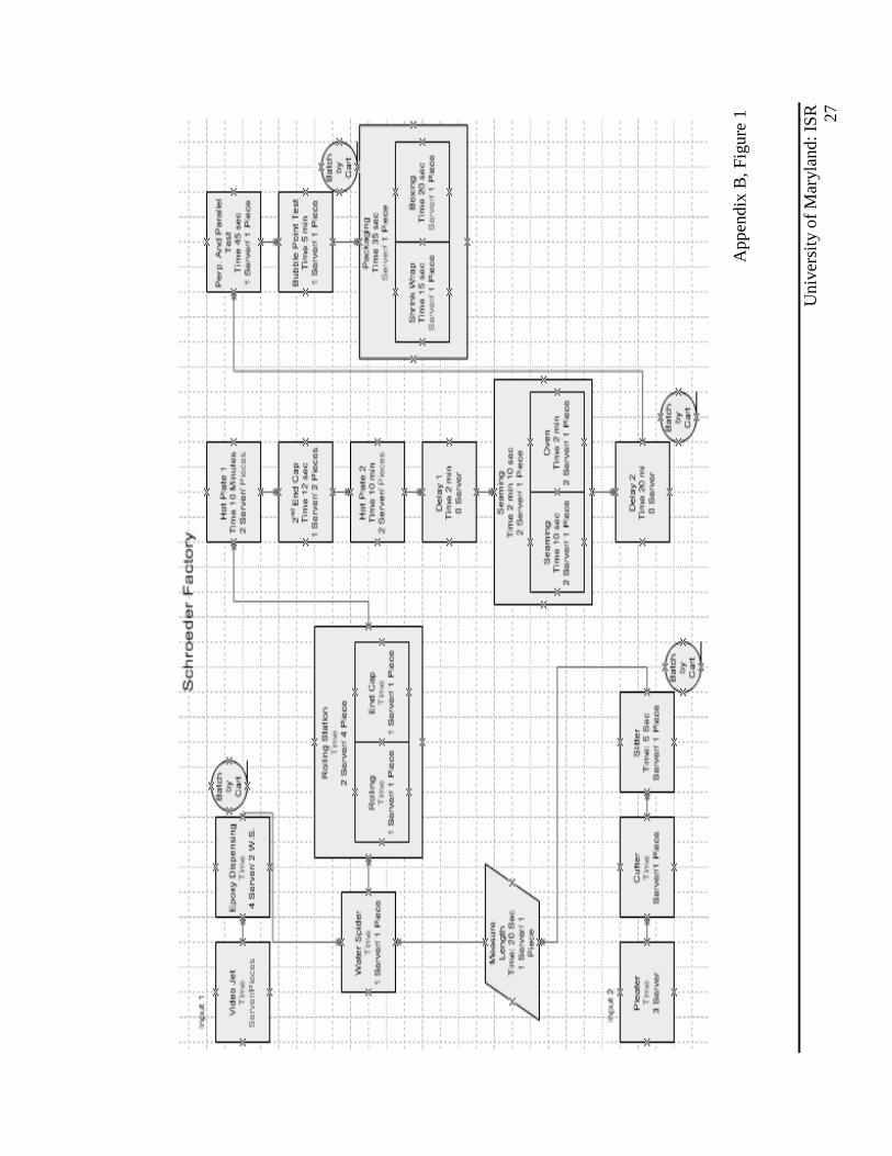
understanding of the data more clearly. (Refer to Appendix B, Figure 1) The flowchart
included the order of the stations that each part went through, the time it takes at each
station, and the number of parts that could be served at one time. We worked with the
existing layout that Schroeder Industries had given us on our visit and our memories of
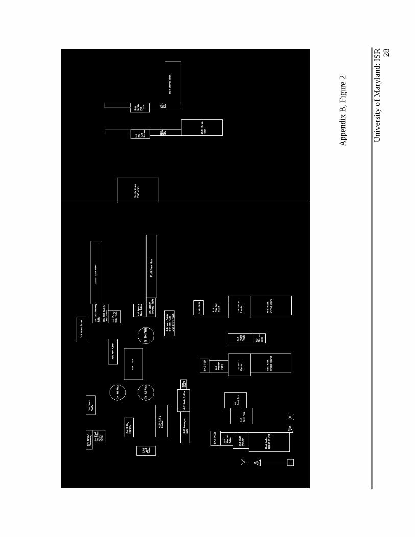
the factory layout to create a new, to-scale CAD drawing of the factory floor. (Refer to
Appendix B, Figure 2) While combining our data and creating these documents we
made sure to highlight all of the information we were missing and also came up with a
list of questions for Schroeder Industries. We emailed them our questions, along with the
CAD drawing and flowchart we had created of the factory to receive more information
and make sure we had a correct understanding of the factory. After hearing back from
Schroeder, we then began to create an animated simulation of the current factory layout
that would include all of the data we had collected over the past few weeks. Due to the
fact that most of the data we were given were averages and approximations, we created a
list of assumptions to follow when designing the simulation.

University of Maryland: ISR
13
Assumptions: • The number of pieces created each working day average about 2,150; but the
number of work orders and size of these work orders varies greatly from day to
day.
• The time difference to create different sized filters is minimal; therefore, we do
not take into account these time differences in the simulation.
• One work order is started and kept together throughout the entire process. It may
be sent through the system in smaller batch sizes but they start all batches of one
work order before starting a batch from a separate work order.
• In our simulation work orders are sent through the factory floor in batches of 50,
the average batch size is actually 63 pieces.
Simulation Set-Up: The creation of filters begins with two separate tasks occurring simultaneously at
opposite sides of the factory. At one side of the factory the end caps have information
printed on them at the video jet printer. There is one employee at this station and one end
cap is printed at a time. Printed caps are cured in an oven for 15 minutes. The average
batch size for the ovens is approximately 250 caps per batch based on the cap size.
Typically whole work orders are moved to the next station. If there is a work order for
500 elements the cap filling station would not receive the caps until all 500 caps are
printed and cured. The epoxy dispensing station would then receive 1000 caps (top and
bottom); 500 printed and 500 plain. The scrap rate on the printed caps is less than 1%.
In our simulation we batch the end caps before they are cured and then un-batch them
once they have finished curing. (Refer to Figure 12)

University of Maryland: ISR
14
Once the caps are sent to the epoxy dispensing machine they are filled with
epoxy. There is only one epoxy dispensing machine, with one employee, but two caps
are filled at once at a 10 second processing time. The batch size at this station would be
twice the work order quantity. For example: if the work order called for 200 elements the
batch size would be 400 (2 end caps per element). On a statistical basis the batch size
would be 125 for the next week (149 work orders, 9,324 total elements scheduled to build
x 2 end caps). The new equipment will have epoxy dispensing stations at each hot plate
and the caps will be filled on the line not off line (4 stations in total). The caps are then
placed on a cart to be taken to the water spider. The water spider is the employee that all
the parts for a work order are together. In our simulation we show the caps being placed
together on the cart by batching them together.
On the other side of the factory floor the mesh packs are being made. There are
three pleater machines that make the mesh packs, two manual and one automatic. The
amount of time for these mesh packs to be created is 45 seconds per sheet. They are then
cut to size. Depending on what the work order requires all of the mesh packs for that
work order are either cut using a band saw or the media length cutter. 97% of the mesh

University of Maryland: ISR
15
packs are cut with the band saw, which takes 15 seconds, and there are two servers which
each cut one piece at a time. The factory also has one media length cutter which cuts the
remaining 3% of the mesh packs. This machine takes time to warm up and then requires
45 seconds for each piece. The advantage of the media cutter is that it creates a cleaner
more precise cut. There is a decision block in the simulation which sends 97% of the
mesh packs to the band saw and 3% to the media length cutter. The mesh packs are not
moved until the quantity required per the work order is complete. Statistically this would
be a batch size of 63. The mesh packs are placed on a cart and taken to another part of
the factory where they measure the length. This takes about 20 seconds for each piece,
and only one mesh pack can be measured at a time. The mesh packs being placed on the
cart is also simulated by a batch block. This way they enter the inspection and leave the
inspection as one batch instead of several separate pieces. (Refer to Figure 13)
The water spider is the next station and is very important in making sure that all
pieces of a work order are together and ready to be assembled. At this station all of the
end caps and mesh packs for a work order are organized on a cart to be sent through the
remainder of the factory floor. The water spider has a copy of that days schedule and
work orders, so he places the appropriate size and number of mesh packs and caps onto
the cart. They are placed together in batch sizes; in our simulation about 50 elements can

University of Maryland: ISR
16
be made with the pieces placed on the cart. To make 50 filters there must be 50 mesh
packs and 100 end caps, since one end cap is placed on each side of the mesh pack. This
station will change once the new equipment is placed in the factory. In our simulation
once the caps and mesh packs arrive at the water spider station they both become un-
batched. There is a decision block which separates the end caps evenly into two groups.
The first group goes to the rolling station and the second group of end caps goes to hot
plate 2. All of the mesh packs are sent to the rolling station. (Refer to Figure 14)
From the water spider the batches are sent to the rolling station. There are two
work stations, and both have two servers. The total amount of time needed at the rolling
station is 20 seconds, and this station is broken into two processes. The first process is
rolling which takes 15 seconds, and there are 2 servers each rolling 1 piece. The second
process at the rolling station is End Caps, where the first end cap is placed on 1 side of
the mesh pack. This process takes 5 seconds and there are 2 servers each placing 1 end
cap on a mesh pack at a time. The rolling station is a continuous process, as elements are
built they are placed on the hot plates. After this station there is about a 3% scrap rate.
The simulation shows these events taking place by using a match block; matching 1 cap
and 1 mesh pack together. There is then a batch block which will make these 2 parts stay

University of Maryland: ISR
17
together permanently throughout the remainder of the simulation. The end cap and mesh
pack combination is then sent to hot plate 1. (Refer to Figure 15)
The next station is hot plate 1. The mesh pack with an end cap on 1 side is placed
on the hot plate to dry the epoxy so that these 2 pieces will stay together. There are 2 hot
plates. Each take about 10 minutes, and have a maximum capacity averaging 45 pieces.
It is now time to place the second end cap onto the mesh pack. There is only 1
server who can do 2 pieces at a time, which takes about 5 seconds. The filters now go
onto hot plate 2 so that the epoxy in the second end cap can dry. Again there are two hot
plates that can hold an average maximum of about 45 pieces, and they each take roughly
10 minutes. All of the assembled elements are batched to show them being placed on the
cart. The delay for cooling takes place and then the elements are un-batched and sent to
seaming. (Refer to Figure 16)

University of Maryland: ISR
18
The next station is seaming which is also broken into 2 processes, seaming and
the oven. The seaming process takes 10 seconds and there are 2 servers each doing one
piece. There are also 2 ovens, which takes about 2 minutes. The oven heats the seam so
that it dries and holds the mesh pack together. This is where the filters come to their
second delay which lasts for 20 minutes. The elements are batched together after they
have been seamed and gone through the ovens for this second delay. They remain
batched for the next process in the simulation. (Refer to Figure 17)
The filters are now placed together on a cart and sent to the parallel and
perpendicularity test. This test takes about 45 seconds and 1 piece is done at a time.
Schroeder Company has found that their product has a 1% Acceptable Quality Level
(AQL), which means statistically 1.5% of their product is defective after the inspection.
They have charts that specify how many elements are to be inspected to reach a 1% AQL
depending on the size of the work order. The next test is the bubble point test which
takes roughly 5 minutes and again only tests 1 piece at a time, and goes by the 1% AQL.
The purpose of this test is to make sure that the filters do not allow too much air to go
through. After the test is finished the elements are un-batched. (Refer to Figure 18)

University of Maryland: ISR
19
The last station the filters are sent to is packaging. The packaging station is
continuous on the first shift and is not in use on the second shift. At this station there are
2 processes, shrink wrapping and boxing. The entire station takes about 35 seconds, and
there is 1 server which packages 1 piece at a time. The first process, shrink wrapping,
takes approximately 15 seconds. The second process, boxing, takes about 20 seconds.
When the entire order is produced and packaged the filters are ready to be sent out. The
factory has found from past results that by the end of entire process there is about a 7%
scrap rate. This station has a dispose block showing that it is the end of the simulation.
(Refer to Figure 19)
(Refer to Appendix B, Figure 3 to see all simulation modules together, Refer to
Appendix B, Figure 4 for Animation)
Future Progress: Unfortunately, we were not able to see the Schroeder project through to
completion. However, we were able to create most of the simulation of the current
factory layout and we were also able to import the CAD drawing into Arena and make
progress on the animation. We finished the first part of the report that will be given to

University of Maryland: ISR
20
Schroeder along with the finished simulation in order to explain how the simulation was
created and the logic and assumptions we used to design it.
Final Reflections:
Overall, we both found this summer’s REU experience to be positive and
rewarding, especially for two Industrial and Systems Engineering students. Having two
different projects that we worked on together gave us a great opportunity to experience
system engineering in two very different ways. The Brooke Grove project gave us both
our first research experience and our first practical operations research assignment,
something we are both sure to come across again in the future. It was a preview of what
graduate school for Industrial Engineering might be like, and it definitely gave us a lot to
consider about our futures. The Schroeder Industries project gave a realistic look into the
kind of job an Industrial and Systems Engineer might have.

University of Maryland: ISR
21
Appendix A
Brooke Grove

U
nive
rsit
y of
Mar
ylan
d: I
SR
22
A
ppen
dix
A, F
igur
e 1

U
nive
rsit
y of
Mar
ylan
d: I
SR
23
A
ppen
dix
A, F
igur
e 2

University of Maryland: ISR
24
Appendix A, Figure 3

University of Maryland: ISR
25
Appendix A, Figure 4
Total Process and Wait Times
0.0000
0.5000
1.0000
1.5000
2.0000
2.5000
3.0000
3.5000
Tot al Time in
Clinic (min)
Tot al
Process Time
(min)
Tot al Wait
Time (min)
80% Capacit y
90% Capacit y
95% Capacit y
Queue Times
0.0000
0.1000
0.2000
0.3000
0.4000
0.5000
0.6000
Greet ing St aging Form Review
(Average)
Dispensing
(Average)
80% Capacit y
90% Capacit y
95% Capacit y
Time Study
0.0000
1.0000
2.0000
3.0000
4.0000
5.0000
6.0000
7.0000
Tot al Time in Clinic
(min)
Ent rance t o End of
Forms
End of Forms t o
Exit
80% Capacit y
90% Capacit y
95% Capacit y
Brooke Grove Result s
Utilization
0%
10%
20%
30%
40%
50%
60%
70%
80%
90%
100%
Greet ing Form Review(Average)
Dispensing(Average)
80% Capacity
90% Capacity
95% Capacity

University of Maryland: ISR
26
Appendix B
Schroeder Industries
U
nive
rsit
y of
Mar
ylan
d: I
SR
27
A
ppen
dix
B, F
igur
e 1
U
nive
rsit
y of
Mar
ylan
d: I
SR
28
App
endi
x B
, Fig
ure
2

U
nive
rsit
y of
Mar
ylan
d: I
SR
29
App
endi
x B
, Fig
ure
3

U
nive
rsit
y of
Mar
ylan
d: I
SR
30
App
endi
x B
, Fig
ure
4

University of Maryland: ISR
31
Acknowledgements:
Thanks to the following people for all of their help during the past ten weeks,
Advisor: Dr. Jeffrey Herrmann
Brooke Grove Clinic: Brad Brochtrup, Ali Pilehvar, Peter Lin
Schroeder Project: Schroeder Industries, Ron Hawkins, Ali Pilehvar, Peter Lin