Isosurface Rendering

B. B. Karki, LSUCSC 7443: Scientific Information Visualization

Isosurface Rendering


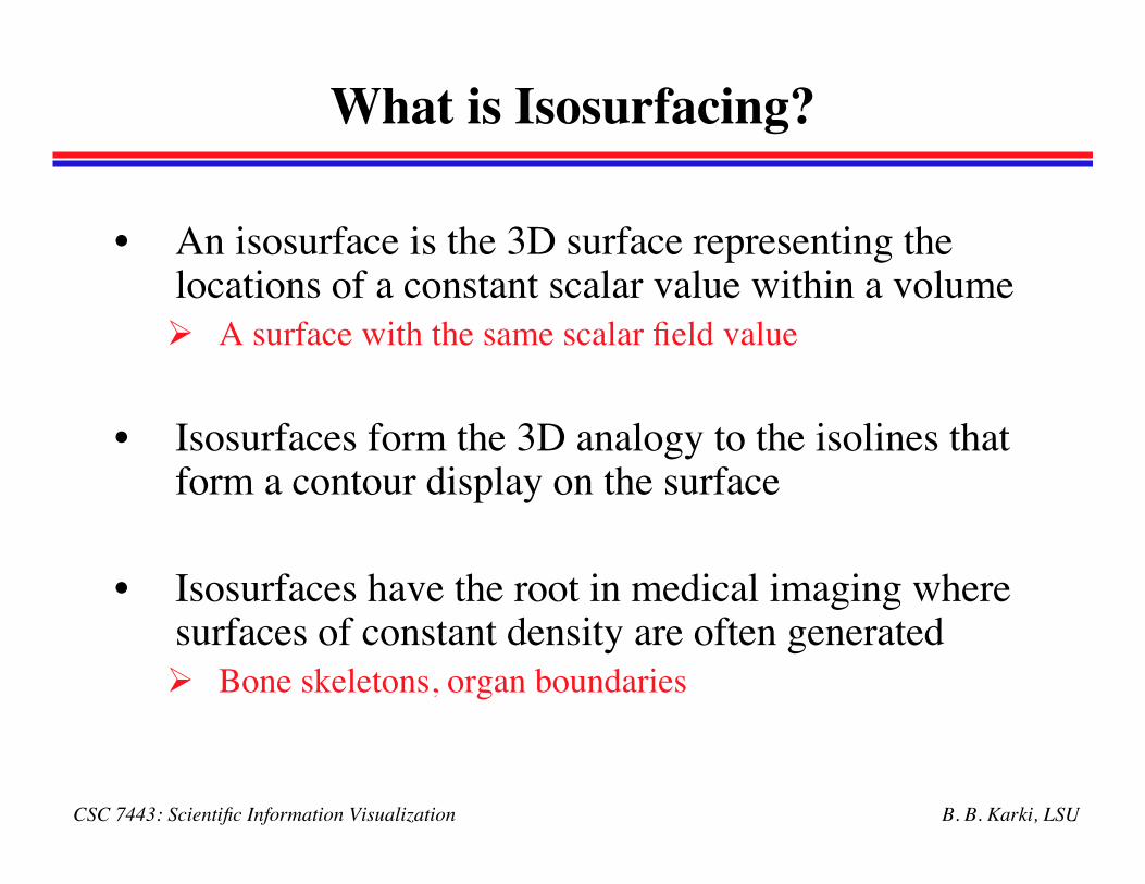
What is Isosurfacing?

• An isosurface is the 3D surface representing thelocations of a constant scalar value within a volume A surface with the same scalar field value

• Isosurfaces form the 3D analogy to the isolines thatform a contour display on the surface

• Isosurfaces have the root in medical imaging wheresurfaces of constant density are often generated Bone skeletons, organ boundaries


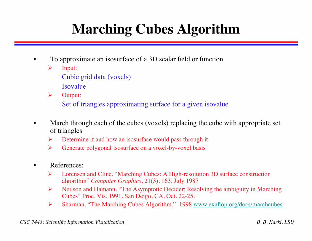
Marching Cubes Algorithm

• To approximate an isosurface of a 3D scalar field or function Input:

Cubic grid data (voxels) Isovalue

Output: Set of triangles approximating surface for a given isovalue

• March through each of the cubes (voxels) replacing the cube with appropriate setof triangles Determine if and how an isosurface would pass through it Generate polygonal isosurface on a voxel-by-voxel basis

• References: Lorensen and Cline, “Marching Cubes: A High-resolution 3D surface construction

algorithm” Computer Graphics, 21(3), 163, July 1987 Neilson and Hamann, “The Asymptotic Decider: Resolving the ambiguity in Marching

Cubes” Proc. Vis. 1991, San Deigo, CA, Oct. 22-25. Sharman, “The Marching Cubes Algorithm,” 1998 www.exaflop.org/docs/marchcubes


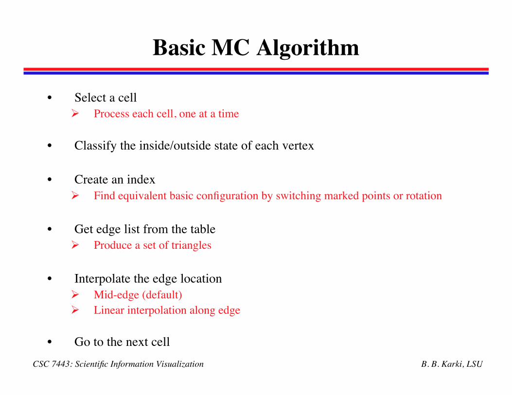
Basic MC Algorithm

• Select a cell Process each cell, one at a time

• Classify the inside/outside state of each vertex

• Create an index Find equivalent basic configuration by switching marked points or rotation

• Get edge list from the table Produce a set of triangles

• Interpolate the edge location Mid-edge (default) Linear interpolation along edge

• Go to the next cell


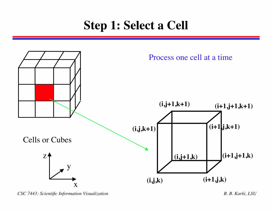
Step 1: Select a Cell

(i,j,k) (i+1,j,k)

(i,j+1,k) (i+1,j+1,k)

(i,j,k+1)

(i,j+1,k+1) (i+1,j+1,k+1)

(i+1,j,k+1)

Cells or Cubes

Process one cell at a time

zy

x


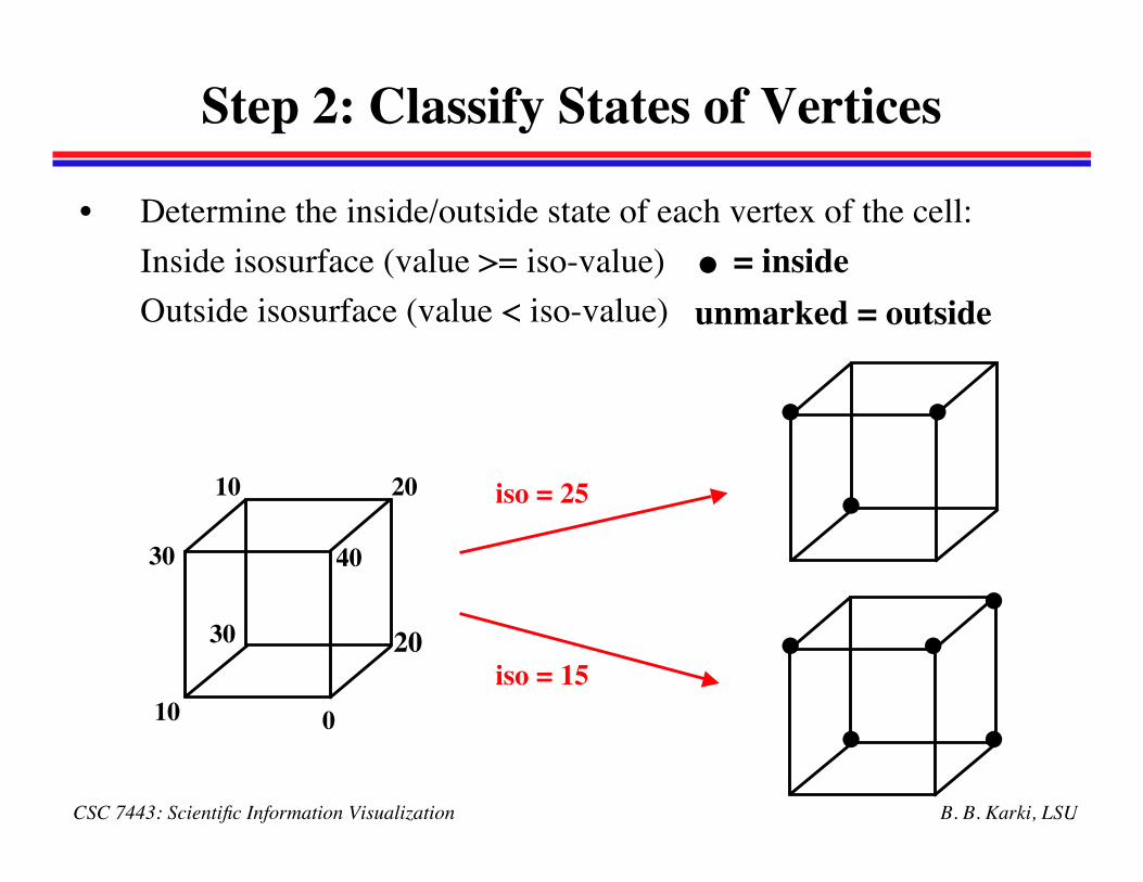
Step 2: Classify States of Vertices

• Determine the inside/outside state of each vertex of the cell:Inside isosurface (value >= iso-value)Outside isosurface (value < iso-value)

10

40

0

30

30

10 20

20iso = 15

iso = 25

• •

•

•••

• •

• = insideunmarked = outside


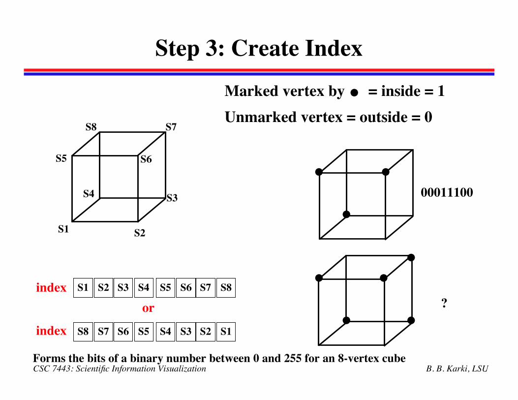
Step 3: Create Index

S1

S6

S2

S4

S5

S8 S7

S3

•

• •

•

•••

• •

Marked vertex by = inside = 1Unmarked vertex = outside = 0

S1 S2 S3 S4 S5 S6 S7 S8

S8 S7 S6 S5 S4 S3 S2 S1

index

indexor

00011100

?

Forms the bits of a binary number between 0 and 255 for an 8-vertex cube


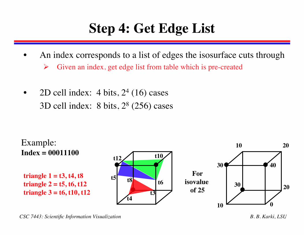
Step 4: Get Edge List

• An index corresponds to a list of edges the isosurface cuts through Given an index, get edge list from table which is pre-created

• 2D cell index: 4 bits, 24 (16) cases3D cell index: 8 bits, 28 (256) cases

• •

•

Example:Index = 00011100

• •

•For

isovalue of 25

10

40

0

30

30

10 20

20

t4t3

t8t5

t12 t10

t6triangle 1 = t3, t4, t8triangle 2 = t5, t6, t12triangle 3 = t6, t10, t12


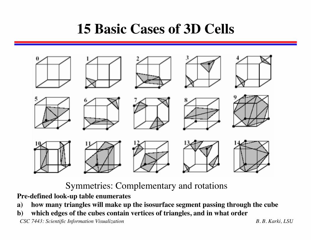
15 Basic Cases of 3D Cells

Symmetries: Complementary and rotationsPre-defined look-up table enumerates a) how many triangles will make up the isosurface segment passing through the cubeb) which edges of the cubes contain vertices of triangles, and in what order


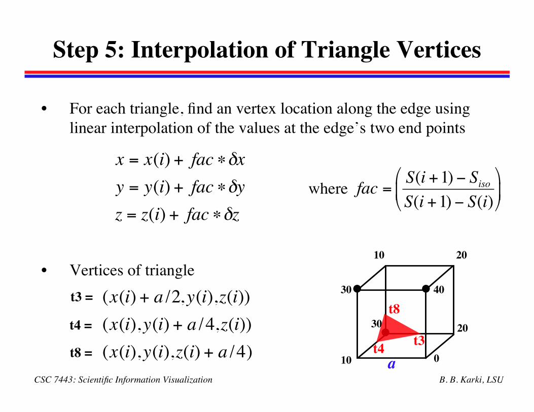
Step 5: Interpolation of Triangle Vertices

• For each triangle, find an vertex location along the edge usinglinear interpolation of the values at the edge’s two end points

!

x = x(i) + fac "#x

y = y(i) + fac "#y

z = z(i) + fac "#z

where

!

fac =S(i +1) " SisoS(i +1) " S(i)

#

$ %

&

' (

• •

•10

40

0

30

30

10 20

20

!

(x(i) + a /2,y(i),z(i))

(x(i),y(i) + a /4,z(i))

(x(i),y(i),z(i) + a /4)

t3 =

t8 =

t4 =t3t4

t8

• Vertices of triangle

a


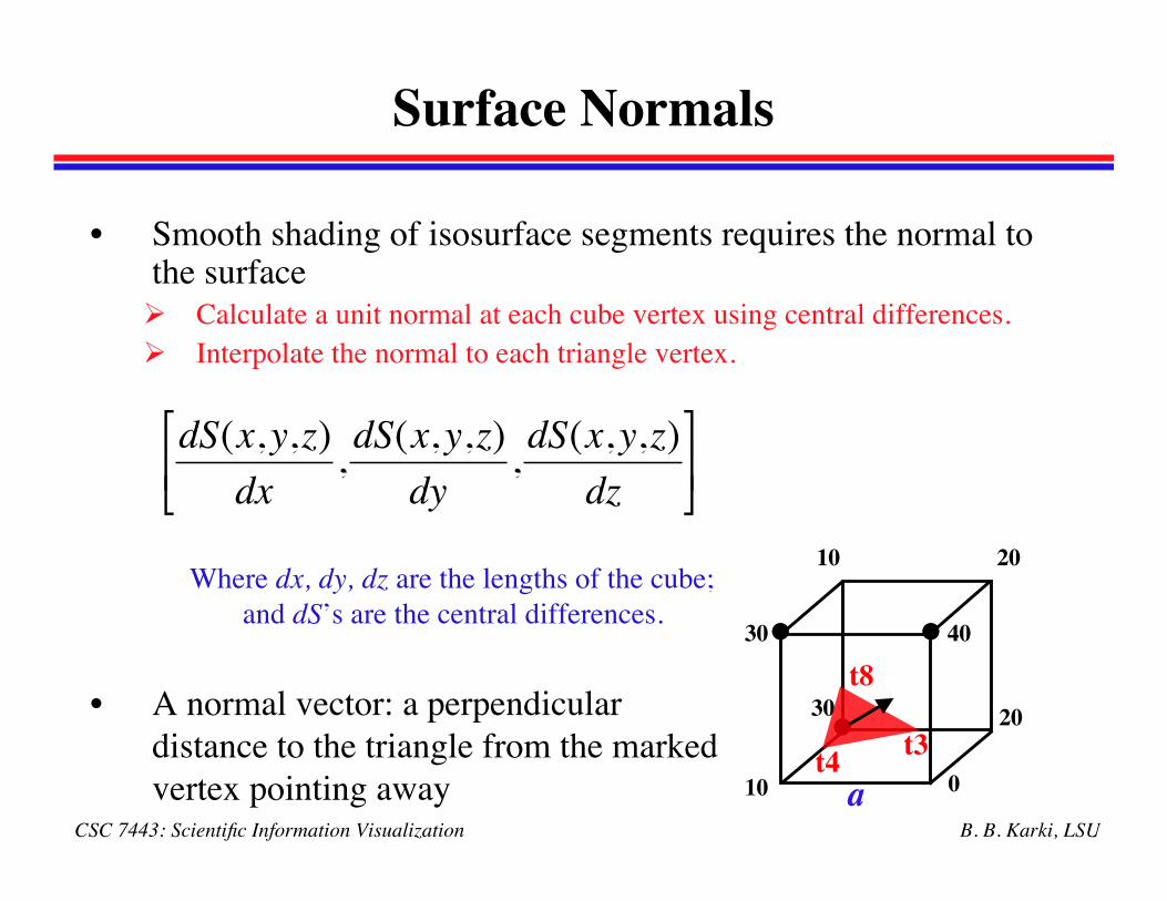
Surface Normals

• Smooth shading of isosurface segments requires the normal tothe surface Calculate a unit normal at each cube vertex using central differences. Interpolate the normal to each triangle vertex.

!

dS(x,y,z)

dx,dS(x,y,z)

dy,dS(x,y,z)

dz

"

# $

%

& '

• •

•10

40

0

30

30

10 20

20t3t4

t8

Where dx, dy, dz are the lengths of the cube;and dS’s are the central differences.

• A normal vector: a perpendiculardistance to the triangle from the markedvertex pointing away a


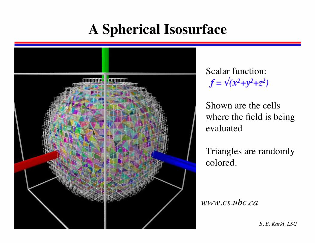
A Spherical Isosurface

www.cs.ubc.ca

Scalar function: f = √(x2+y2+z2)

Shown are the cellswhere the field is beingevaluated

Triangles are randomlycolored.


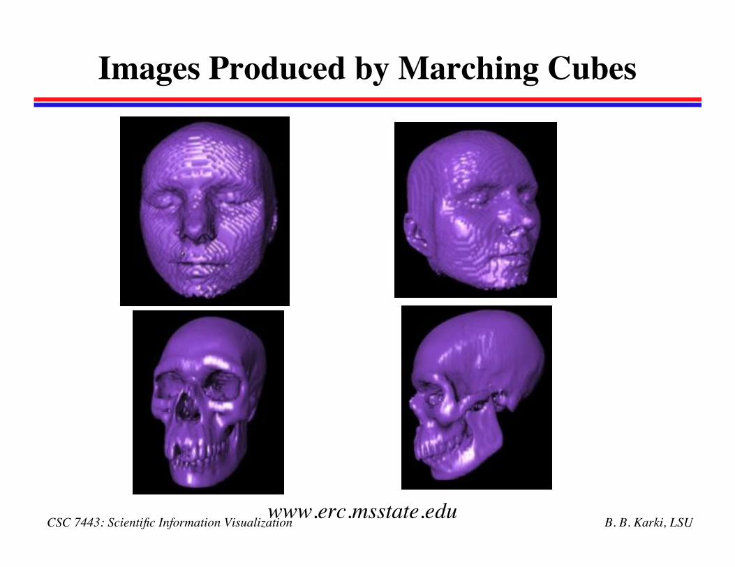
Images Produced by Marching Cubes

www.erc.msstate.edu


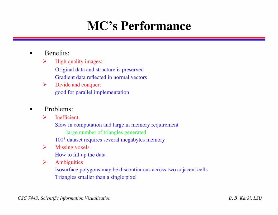
MC’s Performance

• Benefits: High quality images:

Original data and structure is preserved Gradient data reflected in normal vectors

Divide and conquer: good for parallel implementation

• Problems: Inefficient:

Slow in computation and large in memory requirementlarge number of triangles generated

1003 dataset requires several megabytes memory Missing voxels

How to fill up the data Ambiguities

Isosurface polygons may be discontinuous across two adjacent cells Triangles smaller than a single pixel

CSC 7443: Scientific Information Visualization B. B. Karki, LSU

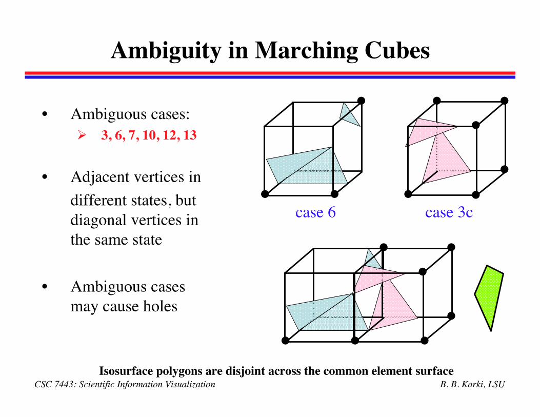
Ambiguity in Marching Cubes

• Ambiguous cases: 3, 6, 7, 10, 12, 13

• Adjacent vertices indifferent states, butdiagonal vertices inthe same state

• Ambiguous casesmay cause holes

••

•

••

•

•case 6 case 3c

Isosurface polygons are disjoint across the common element surface

• •

••

•

••• •


Resolving the Ambiguity

• Using different triangulations, leading toconsistency

Asymptotic deciders

Improved Marching Cubes

Marching tetrahedra


The Asymptotic Decider

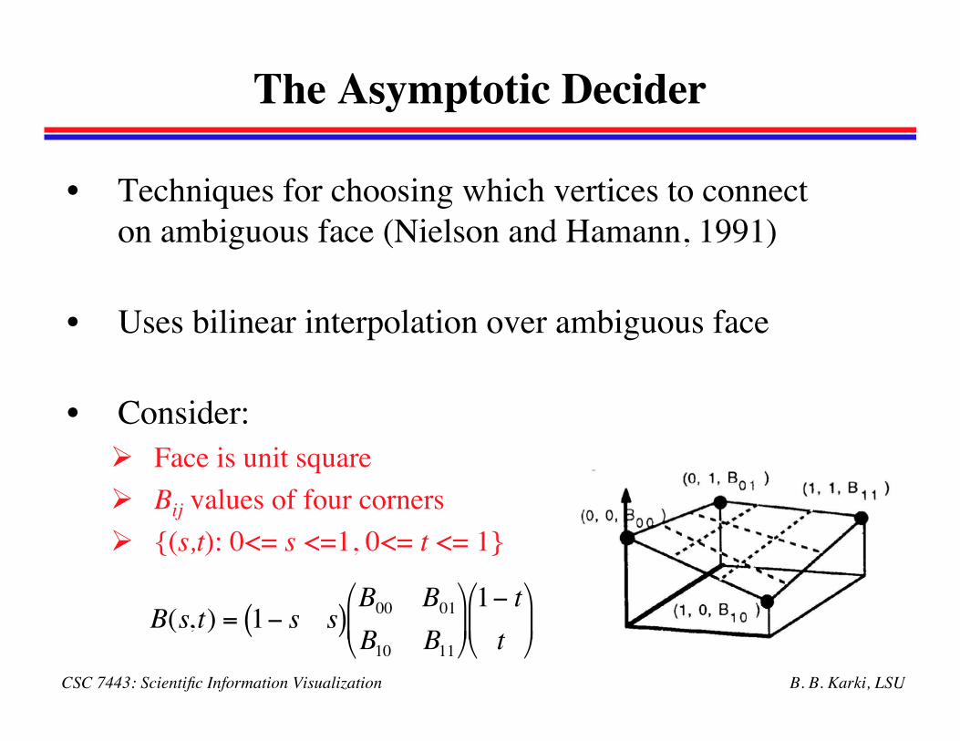
• Techniques for choosing which vertices to connecton ambiguous face (Nielson and Hamann, 1991)

• Uses bilinear interpolation over ambiguous face

• Consider: Face is unit square Bij values of four corners {(s,t): 0<= s <=1, 0<= t <= 1}

!

B(s,t) = 1" s s( )B00

B01

B10

B11

#

$ %

&

' ( 1" t

t

#

$ %

&

' (


AD (Contd.)

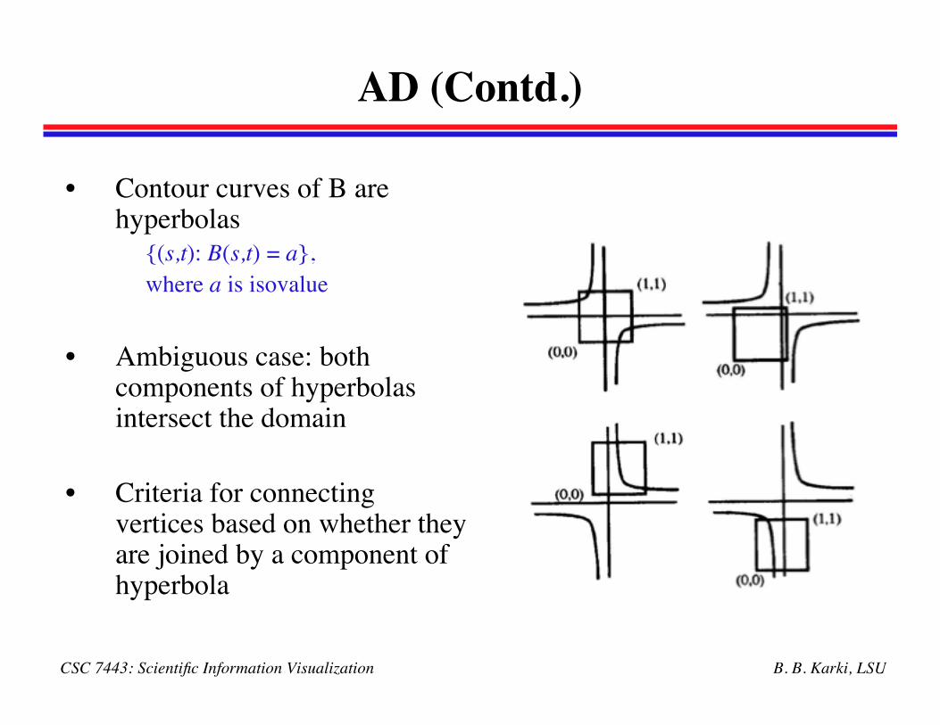
• Contour curves of B arehyperbolas

{(s,t): B(s,t) = a},where a is isovalue

• Ambiguous case: bothcomponents of hyperbolasintersect the domain

• Criteria for connectingvertices based on whether theyare joined by a component ofhyperbola


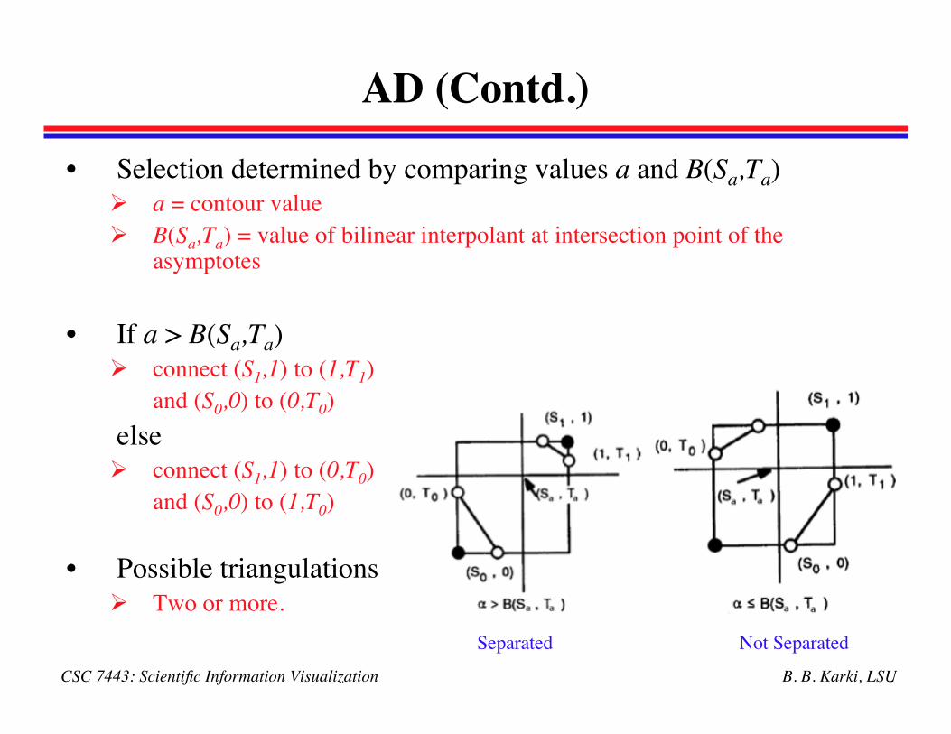
AD (Contd.)• Selection determined by comparing values a and B(Sa,Ta)

a = contour value B(Sa,Ta) = value of bilinear interpolant at intersection point of the

asymptotes

• If a > B(Sa,Ta) connect (S1,1) to (1,T1)

and (S0,0) to (0,T0)else connect (S1,1) to (0,T0)

and (S0,0) to (1,T0)

• Possible triangulations Two or more.

Not SeparatedSeparated


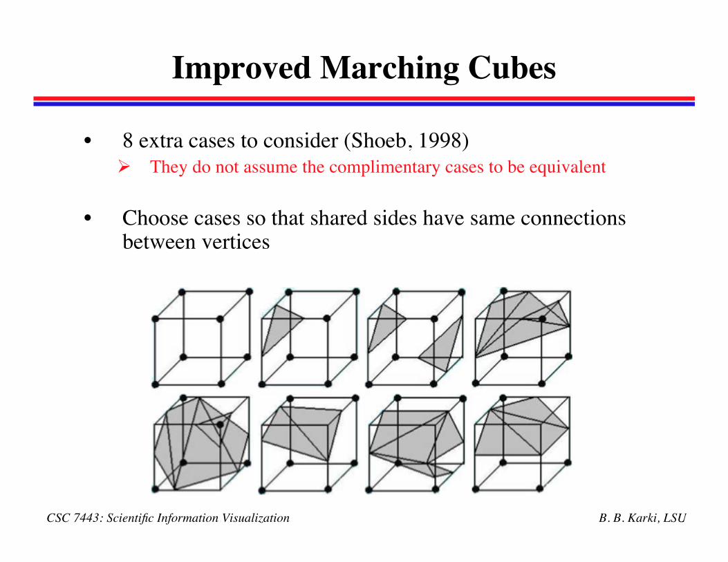
Improved Marching Cubes

• 8 extra cases to consider (Shoeb, 1998) They do not assume the complimentary cases to be equivalent

• Choose cases so that shared sides have same connectionsbetween vertices


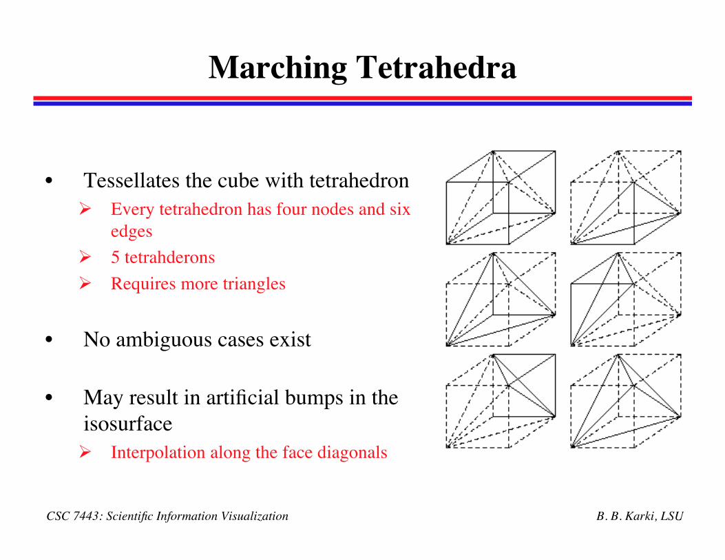
Marching Tetrahedra

• Tessellates the cube with tetrahedron Every tetrahedron has four nodes and six

edges 5 tetrahderons Requires more triangles

• No ambiguous cases exist

• May result in artificial bumps in theisosurface Interpolation along the face diagonals


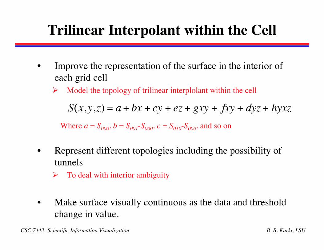
Trilinear Interpolant within the Cell

• Improve the representation of the surface in the interior ofeach grid cell Model the topology of trilinear interplolant within the cell

Where a = S000, b = S001-S000, c = S010-S000, and so on

• Represent different topologies including the possibility oftunnels To deal with interior ambiguity

• Make surface visually continuous as the data and thresholdchange in value.

€

S(x,y,z) = a + bx + cy + ez + gxy + fxy + dyz + hyxz


Implicit Isosurfaces


Particle Sampling

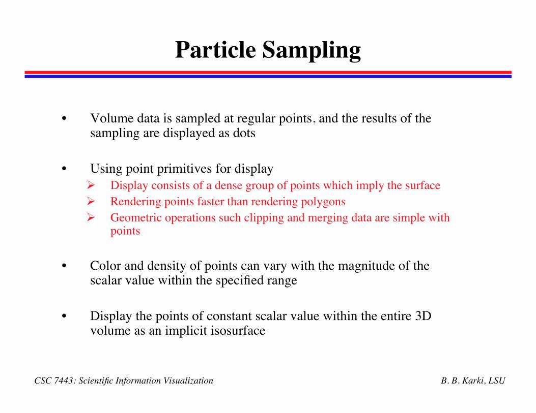
• Volume data is sampled at regular points, and the results of thesampling are displayed as dots

• Using point primitives for display Display consists of a dense group of points which imply the surface Rendering points faster than rendering polygons Geometric operations such clipping and merging data are simple with

points

• Color and density of points can vary with the magnitude of thescalar value within the specified range

• Display the points of constant scalar value within the entire 3Dvolume as an implicit isosurface


Shape Function Interpolation

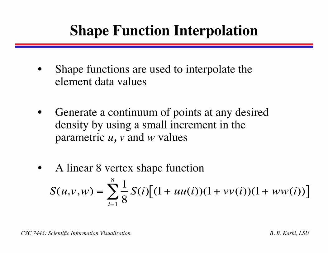
• Shape functions are used to interpolate theelement data values

• Generate a continuum of points at any desireddensity by using a small increment in theparametric u, v and w values

• A linear 8 vertex shape function

!

S(u,v,w) =1

8S(i) (1+ uu(i))(1+ vv(i))(1+ ww(i))[ ]

i=1

8

"


Dividing Cubes Algorithm

• Generates isosurface using dense cloud points

• Use point primitives unlike triangles in Marching Cubes

• Conditions Large number of points Density of points >= screen resolution Lighting and shading calculations

H. Cline, W. Lorensen, S. Ludke, C. Crawford, and B. Teeter, “Twoalgorithms for the three-dimensional reconstruction of tomographs”Medical Physics, vol. 15, no. 3, May 1988


Find Intersecting Voxel

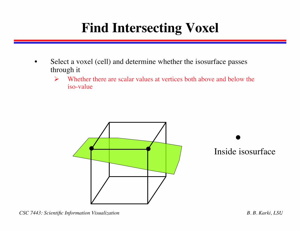
• Select a voxel (cell) and determine whether the isosurface passesthrough it Whether there are scalar values at vertices both above and below the

iso-value

• ••

Inside isosurface


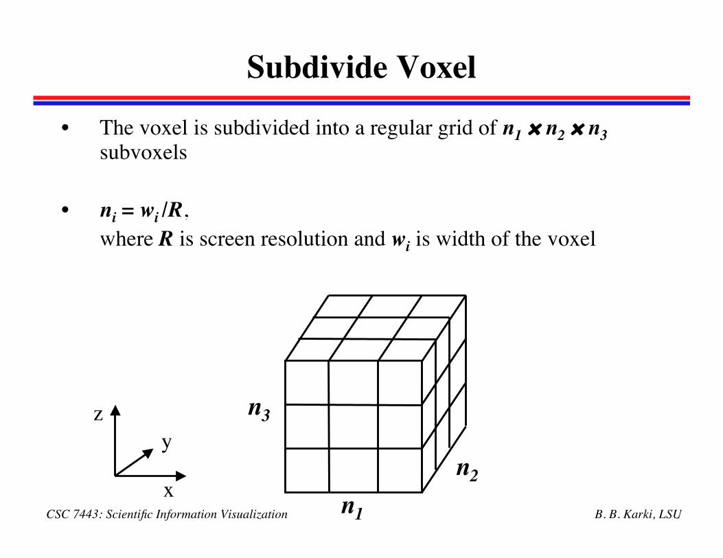
Subdivide Voxel• The voxel is subdivided into a regular grid of n1 × n2 × n3

subvoxels

• ni = wi /R,where R is screen resolution and wi is width of the voxel

zy

xn2

n3

n1


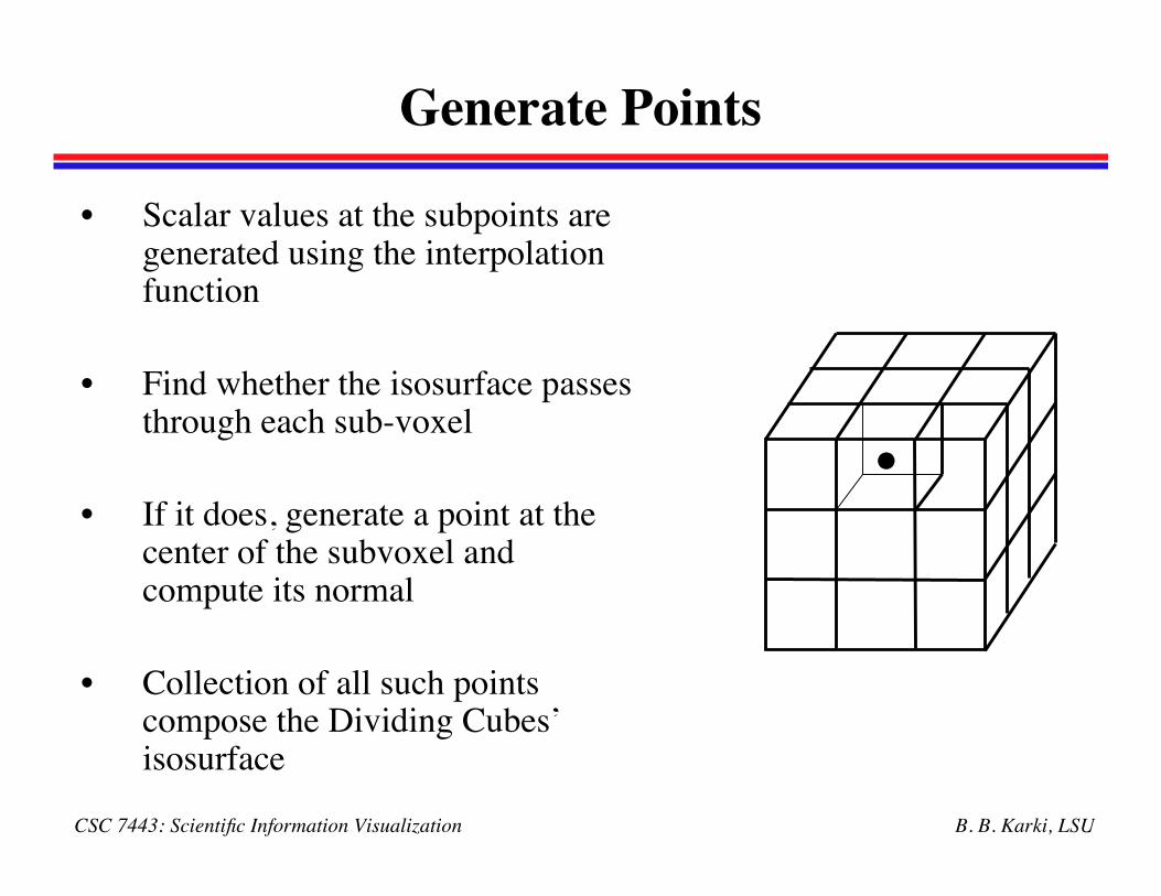
Generate Points

• Scalar values at the subpoints aregenerated using the interpolationfunction

• Find whether the isosurface passesthrough each sub-voxel

• If it does, generate a point at thecenter of the subvoxel andcompute its normal

• Collection of all such pointscompose the Dividing Cubes’isosurface

•


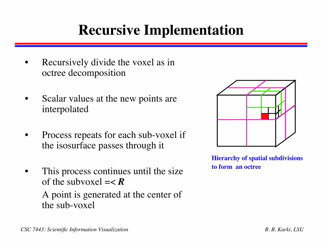
Recursive Implementation

• Recursively divide the voxel as inoctree decomposition

• Scalar values at the new points areinterpolated

• Process repeats for each sub-voxel ifthe isosurface passes through it

• This process continues until the sizeof the subvoxel =< RA point is generated at the center ofthe sub-voxel

Hierarchy of spatial subdivisions to form an octree


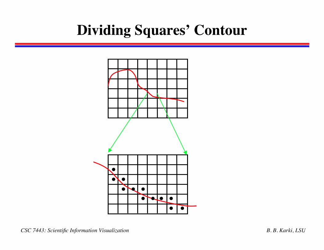
Dividing Squares’ Contour

•• •• • •

• • • •• •


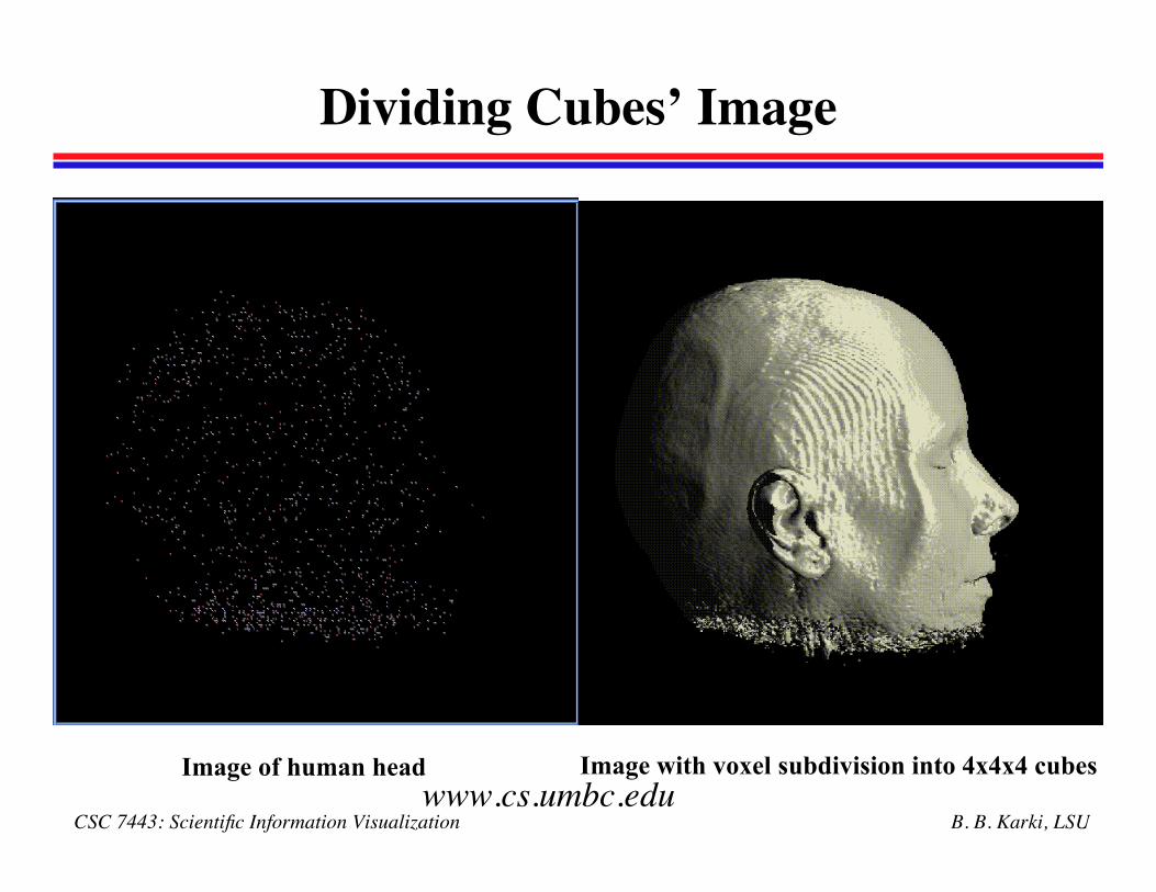
Dividing Cubes’ Image

Image of human head Image with voxel subdivision into 4x4x4 cubeswww.cs.umbc.edu


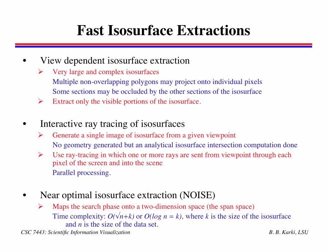
Fast Isosurface Extractions

• View dependent isosurface extraction Very large and complex isosurfaces

Multiple non-overlapping polygons may project onto individual pixels Some sections may be occluded by the other sections of the isosurface

Extract only the visible portions of the isosurface.

• Interactive ray tracing of isosurfaces Generate a single image of isosurface from a given viewpoint

No geometry generated but an analytical isosurface intersection computation done Use ray-tracing in which one or more rays are sent from viewpoint through each

pixel of the screen and into the scene Parallel processing.

• Near optimal isosurface extraction (NOISE) Maps the search phase onto a two-dimension space (the span space)

Time complexity: O(√n+k) or O(log n = k), where k is the size of the isosurfaceand n is the size of the data set.


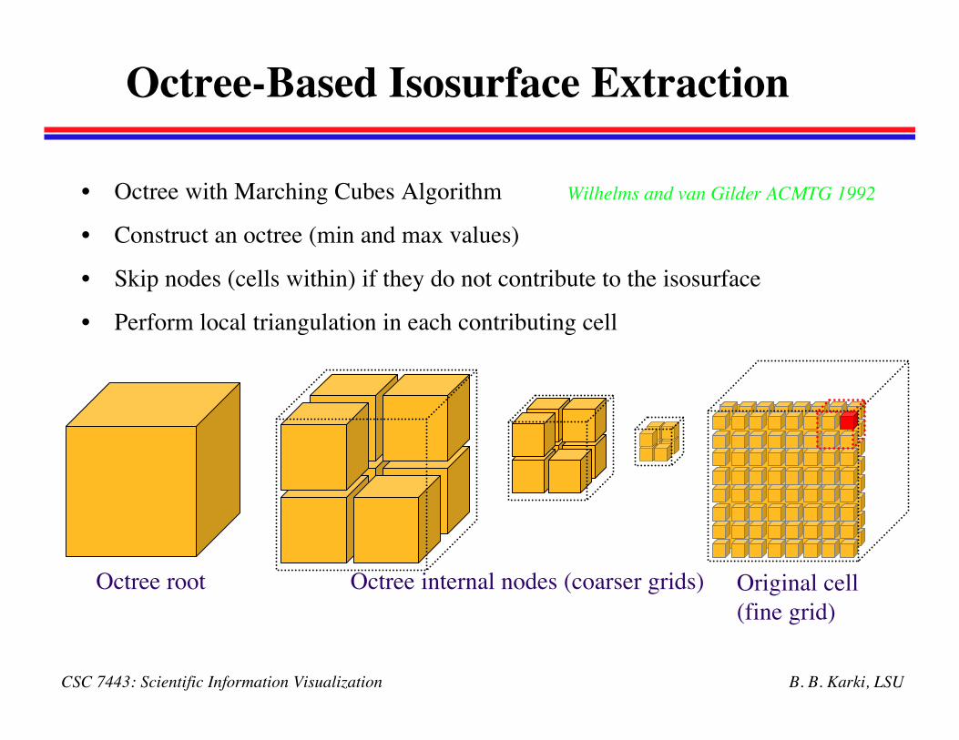
Original cell(fine grid)

Octree internal nodes (coarser grids)

Octree-Based Isosurface Extraction

• Octree with Marching Cubes Algorithm

• Construct an octree (min and max values)

• Skip nodes (cells within) if they do not contribute to the isosurface

• Perform local triangulation in each contributing cell

Octree root

Wilhelms and van Gilder ACMTG 1992


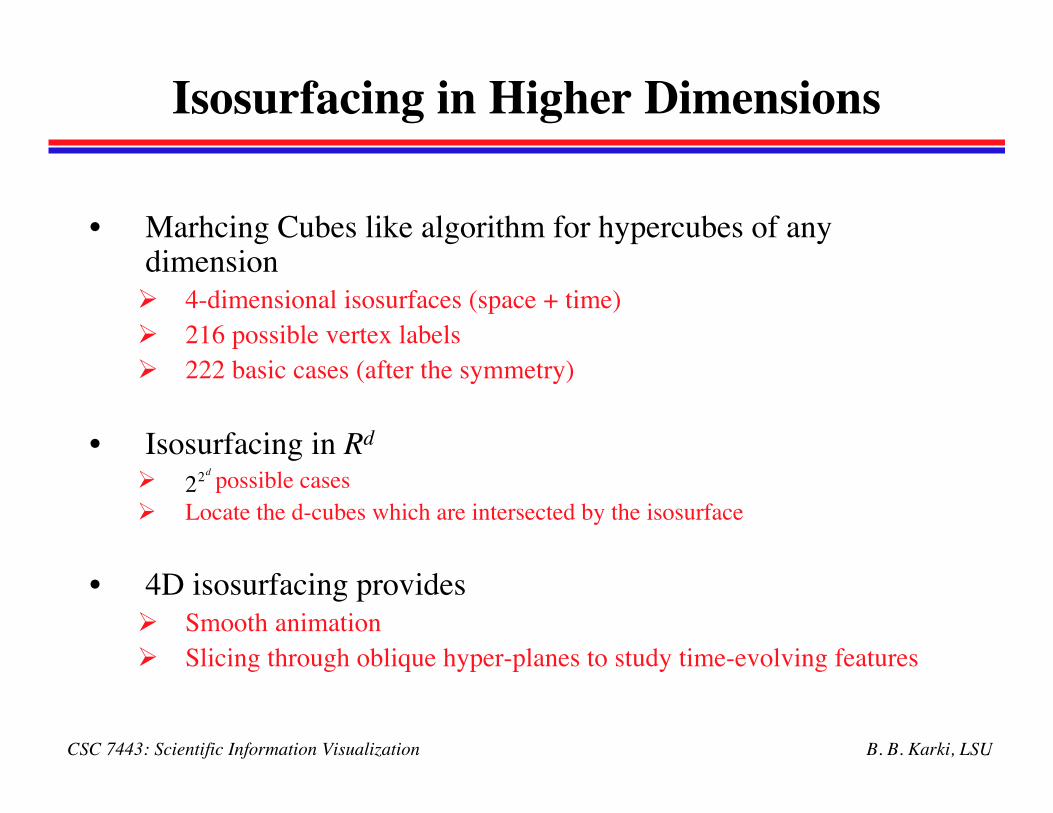
Isosurfacing in Higher Dimensions

• Marhcing Cubes like algorithm for hypercubes of anydimension 4-dimensional isosurfaces (space + time) 216 possible vertex labels 222 basic cases (after the symmetry)

• Isosurfacing in Rd

possible cases Locate the d-cubes which are intersected by the isosurface

• 4D isosurfacing provides Smooth animation Slicing through oblique hyper-planes to study time-evolving features

€

22d

Isosurface Rendering

Documents

Transcript of Isosurface Rendering