Parallel Learning of Koopman Eigenfunctions and Invariant ...

Isostables, isochrons, and Koopman spectrum
for the action-angle representation of stable fixed point dynamics
A. Mauroy,∗ I. Mezic,† and J. Moehlis‡
Department of Mechanical Engineering,
University of California Santa Barbara, Santa Barbara, CA 93106, USA
1

Abstract
For asymptotically periodic systems, a powerful (phase) reduction of the dynamics is obtained by
computing the so-called isochrons, i.e. the sets of points that converge toward the same trajectory
on the limit cycle. Motivated by the analysis of excitable systems, a similar reduction has been
attempted for non-periodic systems admitting a stable fixed point. In this case, the isochrons
can still be defined but they do not capture the asymptotic behavior of the trajectories. Instead,
the sets of interest—that we call “isostables”—are defined in literature as the sets of points that
converge toward the same trajectory on a stable slow manifold of the fixed point. However, it
turns out that this definition of the isostables holds only for systems with slow-fast dynamics.
Also, efficient methods for computing the isostables are missing.
The present paper provides a general framework for the definition and the computation of the
isostables of stable fixed points, which is based on the spectral properties of the so-called Koopman
operator. More precisely, the isostables are defined as the level sets of a particular eigenfunction of
the Koopman operator. Through this approach, the isostables are unique and well-defined objects
related to the asymptotic properties of the system. Also, the framework reveals that the isostables
and the isochrons are two different but complementary notions which define a set of action-angle
coordinates for the dynamics. In addition, an efficient algorithm for computing the isostables is
obtained, which relies on the evaluation of Laplace averages along the trajectories. The method
is illustrated with the excitable FitzHugh-Nagumo model and with the Lorenz model. Finally,
we discuss how these methods based on the Koopman operator framework relate to the global
linearization of the system and to the derivation of special Lyapunov functions.
Keywords: Nonlinear dynamics, isochrons, excitable systems, Koopman operator, action-angle coordinates,
Lyapunov function
∗Electronic address: [email protected]
†Electronic address: [email protected]
‡Electronic address: [email protected]
2

I. INTRODUCTION
Among the abundant literature on networks of coupled systems, a vast majority of studies
focus on asymptotically periodic systems (i.e. coupled oscillators) while only a few consider
coupled systems characterized by a stable fixed point. This is particularly surprising since the
latter can exhibit excitable regimes that are relevant in many situations (e.g. neuroscience
[14]). One reason for this disproportion is probably related to phase reduction methods.
For asymptotically periodic systems, powerful phase reduction methods turn the (complex,
high-dimensional) system into a phase oscillator evolving on the circle, making the analysis
of complex networks more amenable to mathematical analysis [2, 16, 31]. In contrast, in
the case of systems admitting a stable fixed point, the development of equivalent reduction
methods is more recent and a general framework is still in its infancy.
The goal of reduction methods is to assign the same value to a (codimension-1) set of
initial conditions that are characterized by the same asymptotic behavior, in turn designing
a coordinate on the state space. In the case of asymptotically periodic systems, these sets of
identical (phase) value are the so-called isochrons, which approach the same trajectory on
the limit cycle [32]. This concept has been recently extended to heteroclinic cycles [29]. For
systems admitting a stable focus, the isochrons (or isochronous sections) can still be defined
as the sets of points that are invariant under a particular return map [9, 28]. This notion is of
particular interest in the case of weak foci (i.e. with purely imaginary eigenvalues) and non-
smooth vector fields, where the existence of isochrons is a non-trivial problem related to the
stability of the fixed point. However, the isochrons provide in this case no information on the
asymptotic convergence of the trajectories toward the fixed point and are not useful for the
system reduction. (Note also that they do not exist for fixed points with real eigenvalues.)
Therefore, the isochrons must be complemented by another family of sets: the so-called
isostables.
Excitable systems are characterized by slow-fast dynamics with a stable fixed point and,
in the plane, they admit a particular trajectory—the transient attractor or slow manifold—
that temporarily attracts all the trajectories as they approach the fixed point. In this case,
the isostables are naturally defined as the sets of points that converge to the same trajectory
on the transient attractor [24]. (Note that these sets are called “isochrons” in [24], but we
feel that the proper sense is “isostables” instead, in order to avoid the confusion with the
3

isochrons of foci studied in [9, 28].) For non-planar systems possessing a multi-dimensional
slow manifold or center manifold, a (more rigorous) framework was previously developed
in [4, 26]. In that work, the sets of interest (called “projection manifolds” in [26]) are
closely related to the notion of isostable and correspond to the invariant fibers of the (slow
or center) manifold, i.e. the sets of initial conditions characterized by the same long-term
behavior on that manifold. Through the reduction obtained with the isostables, excitable
systems have been studied in various contexts (sensitivity to periodic pulses [3, 13, 25],
network synchronization [17], etc.).
Since the isostables provide a characterization of the system dynamics around the fixed
point, their computation is also desirable for systems which do not contain multiple time
scales (i.e. with no slow or center manifold). For instance, the computation of the isosta-
bles can be useful to achieve an optimal control that minimizes the time of convergence
toward a steady state or to investigate the delay of convergence to a stable equilibrium
in decision-making models [30]. But in these cases, a more general framework is required,
which defines the isostables as particular (and unique) codimension-1 sets capturing the
asymptotic behavior of the system. In addition, the computation of the isostables through
backward integration [24] or normal form of the dynamics [4] is limited to a neighborhood
of the slow manifold. In this context, an efficient method for computing the isostables in
the entire basin of attraction is also missing.
In this paper, we propose a general framework for the reduction of systems admitting a
stable fixed point, which is not limited to excitable systems with slow-fast dynamics. This
approach is based on the spectral properties of the so-called Koopman operator [19, 21].
More precisely, we propose a general and unique definition of the isostables in terms of a
particular eigenfunction of the Koopman operator. In addition, the framework yields an
efficient method to compute the isostables in the whole basin of attraction. This method
relies on the estimation of Laplace averages along the trajectories and can be seen as an
extension of the approach recently developed in [18] to compute the isochrons of limit cycles.
Viewed through the Koopman operator framework, the isostables and the isochrons ap-
pear to be two different but complementary concepts. On the one hand, they are different
since they are related to the absolute value and to the argument, respectively, of the eigen-
function of the Koopman operator. On the other hand, they are complementary in the sense
that they define a set of action-angle coordinates for the system dynamics. This action-angle
4

representation is related to important properties of the isotables, such as the global lineariza-
tion of the dynamics and the derivation of special Lyapunov functions, that we discuss in
the paper.
The paper is organized as follows. In Section II, we introduce the concept of isostable in
the context of the Koopman operator framework, both for linear and nonlinear systems. We
also propose a rigorous definition of the isostables and discuss their main properties. The
relation between the isostables and the Laplace averages is developed in Section III. This
provides an efficient algorithm for the computation of the isostables which is illustrated in
Section IV for the excitable FitzHugh-Nagumo model and the Lorenz model. Finally, the
related concepts of action-angle representation, global linearization, and Lyapunov function
are discussed in Section V. Section VI gives some concluding remarks.
II. ISOSTABLES AND KOOPMAN OPERATOR
The isostables of an asymptotically stable fixed point x∗ are the sets of points that share
the same asymptotic convergence toward the fixed point. More precisely, trajectories with
an initial condition on an isostable Iτ0 simultaneously intersect the successive isostables Iτn
after a time interval τn − τ0, thereby approaching the fixed point synchronously (Figure
1). The isostables partition the basin of attraction of the fixed point and define a new
coordinate τ that satisfies τ = 1 along the trajectories. Or equivalently, they define a
coordinate r , exp(λτ) with the linear dynamics r = λr. This new coordinate can be used
in a context of model reduction.
At this point, it is important to remark that this (intuitive) definition of isostable is not
complete. Indeed, there exist an infinity of families of sets that satisfy the above-described
property. But among these families, only one defines a smooth change of coordinates and
is relevant to capture the asymptotic behavior of the trajectories. In this section, we will
give a rigorous definition of this unique family of isostables. To do so, we first consider the
particular case of linear systems. Then, we extend the concept to nonlinear systems, using
the Koopman operator framework.
5

Figure 1: Trajectories starting from the same isostable Iτ0 are characterized by the same con-
vergence toward the fixed point. They simultaneously intersect the successive isostables Iτn and
approach the fixed point synchronously.
A. Linear systems
Consider the stable linear system
x = Ax , x ∈ Rn , (1)
and assume that each eigenvalue λj = σj + iωj of the matrix A is of multiplicity 1, has
a strictly negative real part σj < 0, and corresponds to the right eigenvector vj (which is
normalized, that is, ‖vj‖ = 1). By convention, we sort the eigenvalues so that λ1 is the
eigenvalue related to the “slowest” direction, that is
σj ≤ σ1 < 0 , j = 2, . . . , n . (2)
The flow induced by (1) is the continuous-time map φ : R×Rn 7→ Rn, that is, φ(t, x) is the
solution of (1) with the initial condition x. For linear systems, the flow is given by
φ(t, x) =n∑
j=1
sj(x)vj eλjt , (3)
where sj(x) are the coordinates of the vector x in the basis (v1, . . . , vn). The function sj(x)
can be computed as the inner product sj(x) = 〈x, vj〉, with vj the eigenvectors of the adjoint
A∗, associated with the eigenvalues λcj = σj −iωj and normalized so that 〈vj , vj〉 = 1. (Note
that sj(x) is an eigenfunction of the so-called Koopman operator; see Section II B.)
Next, we show that the isostables of linear systems are simply defined as the level sets of
|s1(x)| = |〈x, v1〉|. We consider separately the cases λ1 real (with other eigenvalues real or
complex) and λ1 complex (with other eigenvalues real or complex).
6

1. Real eigenvalue λ1
When the eigenvalue λ1 = σ1 is real, the trajectories induced by the flow (3) asymp-
totically approach the fixed point along the slowest direction v1 (since the eigenvalues
are sorted according to (2)). Then, the trajectories characterized by the same coefficient
|s1(x)| , exp(σ1τ(x)) exhibit the same asymptotic convergence toward the fixed point:
φ(t, x) = v±1 eσ1(t+τ(x)) +
n∑
j=2
sj(x) vj exp(λjt) ≈ v±1 eσ1(t+τ(x)) as t → ∞ , (4)
where the notation v±1 implies that either the vector v1 or −v1 must be considered. The
initial conditions x of these trajectories therefore belong to the same isostable
Iτ =
x ∈ Rn∣
∣
∣
∣
x = eσ1τ v±1 +
n∑
j=2
αj vj , ∀αj ∈ R
, (5)
which is obtained by considering t = 0 in (4). In this case, the isostables are the (n − 1)-
dimensional hyperplanes parallel to vj for all j > 2 (or equivalently, perpendicular to v1)
(Figure 2).
(a) (b)
Figure 2: (a) The isostables of linear systems with a real eigenvalue λ1 are the hyperplanes spanned
by the eigenvectors vj , with j > 2. The particular isostable I∞ contains the fixed point. (b) For
two-dimensional systems (or in the plane v1 − v2), the isostables are pairs of parallel lines.
7

2. Complex eigenvalue λ1
A system having a complex eigenvalue λ1 can be transformed through the use of action-
angle coordinates. Then, the isostables are obtained from the isostables (5) of the subsystem
which is related to the action coordinates and which is only characterized by real eigenvalues
σj . Consider a linear coordinate transformation that expresses the dynamics (1) in the
(spectral) basis given by the vectors vj (for λj real) and ℜ{vj}, −ℑ{vj} (for λj = λcj+1
complex). (Note that ℜ{vj} and ℑ{vj} are not parallel since the two eigenvectors vj
and vj+1 are independent.) This is performed by diagonalizing A and by using the linear
transformation
T =
1 1
−i i
in each subspace spanned by a pair of complex eigenvectors (vj ,vj+1). The dynamics become
yj = σjyj j ∈ {i ∈ {1, . . . , n}|λi ∈ R} ,
yj
yj+1
=
σj −ωj
ωj σj
yj
yj+1
j ∈ {i ∈ {1, . . . , n}|λi = λci+1 /∈ R} ,
with the initial conditions yj(0) = sj(x0) (for λj ∈ R) and (yj(0), yj+1(0)) =
(2ℜ{sj(x0)}, 2ℑ{sj(x0)}) (for λj = λcj+1 /∈ R). Then, using the variables rj = yj (for
λj ∈ R) and the polar coordinates (yj, yj+1) = (rj cos(θj), rj sin(θj)) (for λj = λcj+1 /∈ R), we
obtain the canonical equations
rj = σjrj j ∈ {i ∈ {1, . . . , n}|λi ∈ R or λi = λci+1 /∈ R} , (6)
θj = ωj j ∈ {i ∈ {1, . . . , n}|λi = λci+1 /∈ R} . (7)
The initial conditions are given by rj(0) = sj(x0) (for λj ∈ R) and (rj(0), θj(0)) =
(2|sj(x0)|,∠sj(x0)) (for λj = λcj+1 /∈ R), where ∠ denotes the argument of a complex
number.
According to (6)-(7), the variables rj and θj can be interpreted as the action-angle co-
ordinates of the system (see [1]) and the convergence toward the fixed point is captured by
the (action) variables rj . Therefore, the isostables of (1) correspond to the isostables of the
linear system (6) with the real eigenvalues σj . Since the highest eigenvalue is σ1, the results
of Section II A 1 imply that the isostables are characterized by a constant value |r1|, that
8

is, they are the level sets of |s1(x)|. Denoting r1 = 2|s1(x)| , exp(σ1τ(x)) and using an
expression similar to (5), we obtain (in the variables yi)
Iτ =
y ∈ Rn
∣
∣
∣
∣
y = (cos(θ)e1 + sin(θ)e2)eσ1τ +n∑
j=3
αj ej , ∀αj ∈ R, ∀θ ∈ [0, 2π)
,
where ej are the unit vectors of Rn, or equivalently (in the variables xi)
Iτ =
x ∈ Rn∣
∣
∣
∣
x = (cos(θ)a + sin(θ)b)eσ1τ +n∑
j=3
αj vj , ∀αj ∈ R, ∀θ ∈ [0, 2π)
, (8)
with a = ℜ{v1} and b = −ℑ{v1}. In this case, the isostables are the (n − 1)-dimensional
cylindrical hypersurfaces parallel to vj for all j ≥ 3. The intersection of an isostable with
the 2-dimensional plane spanned by (a, b) (i.e., the base of the cylinder) is an ellipse (Figure
3). Indeed, a linear transformation turns the circle in the variables yj into an ellipse in the
variables xj .
The trajectories starting from the same isostable converge to the fixed point along a spiral
characterized by the vectors (a, b), according to
φ(t, x) ≈ (a cos(ω1t + θ(x)) + b sin(ω1t + θ(x))) eσ1(t+τ(x)) as t → ∞ ,
with exp(σ1τ(x)) = 2|s1(x)| and θ(x) = ∠s1(x). Note that the phase—or angle coordinate—
θ is related to the notion of isochron (see e.g. [9, 28] and Section V).
(a) (b)
Figure 3: (a) The isostables of linear systems with a complex eigenvalue λ1 are cylindrical hyper-
surfaces spanned by vj for all j ≥ 3. (b) For two-dimensional linear systems (or in the plane a−b),
the isostables are ellipses with constant axes.
9

The expressions (5) and (8) provide a unique definition of the isostables in the case of
linear systems, when λ1 is real and when λ1 is complex, respectively. Since v±1 = v1 exp(iθ)
with θ = {0, π} and cos(θ)a + sin(θ)b = ℜ{v1 exp(iθ)}, these two definitions can be sum-
marized in a single definition.
Definition 1 (Isostables of linear systems). For the system (1), the isostable Iτ associated
with the time τ is the (n − 1)-dimensional manifold
Iτ =
x ∈ B(x∗)
∣
∣
∣
∣
x = ℜ{
v1 eiθ}
eσ1τ +n∑
j=j
αj vj , ∀αj ∈ R, ∀θ ∈ Θ
,
with Θ = {0, π} and j = 2 if λ1 ∈ R, and Θ = [0, 2π) and j = 3 if λ1 /∈ R.
B. Nonlinear systems
Now, we consider a nonlinear system
x = F(x) , x ∈ Rn (9)
where F is an analytic vector field, which admits a stable fixed point x∗ with a basin of
attraction B(x∗) ⊆ Rn. In addition, we assume that the Jacobian matrix J computed at
x∗ has n distinct (nonresonant) eigenvalues λj = σj + iωj characterized by strictly negative
real parts σj < 0 and sorted according to (2). (For unstable fixed points or for multiple
eigenvalues, see Remark 1 and Remark 2, respectively.)
The isostables of linear systems have been defined as the level sets of the coefficient s1(x)
that appears in the expression of the flow (3). For nonlinear systems, an expression of the
flow similar to (3) can be obtained through the framework of Koopman operator [19, 21]. The
Koopman semigroup of operators U t describes the evolution of a (vector-valued) observable
f : Rn 7→ Cm along the trajectories of the system and is rigorously defined as the composition
U tf(x) = f ◦φ(t, x). Throughout the paper, we will make no assumption on the observables,
except that they are analytic in the neighborhood of the fixed point. In the space of analytic
observables, the operator has only a point spectrum and its spectral decomposition yields
[20]
U tf(x) =∑
{k1,...,kn}∈Nn
sk11 (x) · · · skn
n (x) vk1···kne(k1λ1+···+knλn)t . (10)
10

A detailed derivation of the decomposition in the case of a stable fixed point is given in Ap-
pendix A. The functions sj(x), j = 1, . . . , n, are the smooth eigenfunctions of U t associated
with the eigenvalues λj, i.e.
U tsj(x) = sj(φ(t, x)) = sj(x)eλjt , (11)
and the vectors vk1···knare the so-called Koopman modes [27], i.e. the projections of the
observable f onto sk11 (x) · · · skn
n (x). For the particular observable f(x) = x, (10) corresponds
to the expression of the flow and can be rewritten as
φ(t, x) = U tx = x∗ +n∑
j=1
sj(x)vj eλjt +∑
{k1,...,kn}∈Nn0
k1+···+kn>1
sk11 (x) · · · skn
n (x) vk1···kne(k1λ1+···+knλn)t .
(12)
The first part of the expansion is similar to the linear flow (3). The eigenvalues λj and the
Koopman modes vj are the eigenvalues and eigenvectors of J, respectively. Although the
eigenfunctions sj(x) are not computed as the inner products 〈x, vj〉 as in the linear case,
they can be interpreted as the inner products 〈z, vj〉, where z is the initial condition of a
virtual trajectory evolving according to the linearized dynamics z = Jz and characterized
by the same asymptotic evolution as φ(t, x) [15]. The other terms in (12) do not appear in
the expression of the linear flow (3) and account for the transient behavior of the trajectories
owing to the nonlinearity of the dynamics.
The isostables can be rigorously defined as the level sets of the absolute value of the
eigenfunction |s1(x)|. Indeed, the asymptotic evolution of the flow (12) is dominated by
the first mode associated to λ1. Then, a same argument as in Section II A shows that the
points x characterized by the same value |s1(x)| are the initial conditions of trajectories that
converge synchronously to the fixed point, with the evolution
φ(t, x) ≈
x∗ + v±1 eσ1(t+τ(x)) , eσ1τ(x) = |s1(x)| , λ1 ∈ R ,
x∗ + ℜ{
v1 ei(ω1t+θ(x))}
eσ1(t+τ(x)) , eσ1τ(x) = 2|s1(x)| , θ(x) = ∠s1(x) λ1 /∈ R .
(13)
We are now in position to propose a general definition for the isostables of a fixed point,
which is valid both for linear and nonlinear systems and which is reminiscent of the usual
definition of isochrons for limit cycles [10, 32].
11

Definition 2 (Isostables). For the system (9), the isostable Iτ of the fixed point x∗, asso-
ciated with the time τ , is the (n − 1)-dimensional manifold
Iτ ={
x ∈ B(x∗)∣
∣
∣
∣
∃ θ ∈ Θ s.t. limt→∞
e−σ1t∥
∥
∥φ(t, x) − x∗ − ℜ{
v1 ei(ω1t+θ)}
eσ1(t+τ)∥
∥
∥ = 0}
,
with Θ = {0, π} and ω1 = 0 if λ1 ∈ R and Θ = [0, 2π) if λ1 /∈ R.
The reader will easily verify that, for all x belonging to the same isostable, Definition 2
imposes the same value |s1(x)| in the decomposition of the flow (12) and the same asymptotic
behavior (13). Note that without the multiplication by the increasing exponential e−σ1t, one
would have Iτ = B(x∗) ∀τ since φ(t, x) − x∗ → 0 as t → ∞ for all x ∈ B(x∗).
Except for the case of multiple eigenvalues, for which v1 might not be unique (see Remark
2), the isostables are uniquely defined through Definition 2. Uniqueness of the isostables also
follows from the fact that the Koopman operator has a unique eigenfunction s1(x) which is
continuously differentiable in the neighborhood of the fixed point. Since it is precisely this
eigenfunction s1(x) that appears in (12), the isostables are the only sets that are relevant
to capture the asymptotic behavior of the trajectories.
Remark 1 (Unstable fixed point). Definition 2 is easily extended to unstable fixed points
characterized by σj > σ1 > 0 for all j. Indeed, the isostables are still given by Definition
2, where the limit t → ∞ is replaced by t → −∞, that is, one considers the flow φ(−t, x)
induced by the (stable) backward-time system. In this case, the isostables are related to the
unstable eigenfunction s1(x) of the Koopman operator.
Remark 2 (Multiple eigenvalues). When the eigenvalue λ1 has a multiplicity m > 1, the
fixed point is either a star node (m linearly independent eigenvectors) or a degenerate node
(m linearly dependent eigenvectors). In the case of a star node, Definition 2 is not unique
since it depends on the direction of the eigenvector v1 (in other words, a C1 eigenfunction
of the Koopman operator corresponding to the eigenvalue λ1 is not unique). Actually, v1
should be replaced in Definition 2 by any linear combination of m orthonormal eigenvectors
of λ1, a situation where the isostables lying in the vicinity of the fixed point correspond to
cylindrical hypersurfaces whose intersection with the hyperplane spanned by the eigenvectors
of λ1 is a hypersphere. In the case of a degenerate node, the asymptotic evolution toward the
fixed point is dominated by the (slowest) term s1(x)v1 tm−1 exp(σ1t). Then, the increasing
exponential exp(−σ1t) in Definition 2 must be replaced by t1−m exp(−σ1t).
12

C. Some remarks on the isostables
Equivalent definitions for excitable systems. In [24], the authors considered two-
dimensional excitable systems characterized by a transient attractor (i.e. slow manifold)
which attracts all the trajectories as they approach the fixed point. They defined the isosta-
bles (they actually used the term “isochrons”, see Section V A) as the sets of points that
converge to the same trajectory on the transient attractor. This definition is equivalent to
Definition 2 since both impose that trajectories on the same isostable have the same asymp-
totic behavior (see also Section IV A). However, the definition of [24] is qualitative since no
trajectory effectively reaches the transient attractor (which may even lose its normal stabil-
ity property near a fixed point with complex eigenvalues). Also, it is valid only if the system
admits a transient attractor induced by the slow-fast dynamics. In contrast, Definition 2 is
more general and does not rely on the existence of a transient attractor.
For systems with a slow (or center) manifold, the “projection manifolds” studied in [4, 26]
are related to the isostables. They are the sets of initial conditions for which the trajectories
share the same long-term behavior on the slow manifold. In addition, they can be obtained
through the normal form of the dynamics [4]. If the slow manifold is one-dimensional and
if λ1 is real, the projection manifolds are identical to the isostables. Otherwise, they do not
exactly correspond to the isostables since they are not related to the slowest direction v1
only and are not of codimension-1.
Isostables and flow. The flow φ(∆t, ·) maps the isostable Iτ to the isostable Iτ+∆t, for
all ∆t ∈ R (as explained in the beginning of Section II). Indeed, if x ∈ Iτ , Definition 2
implies that
limt→∞
e−σ1t∥
∥
∥φ(t, x) − x∗ − ℜ{
v1 ei(ω1t+θ)}
eσ1(t+τ)∥
∥
∥ = 0
for some θ ∈ Θ. Using the substitution t = t′ + ∆t, we have
limt′→∞
e−σ1t′
∥
∥
∥φ (t′, φ(∆t, x)) − x∗ − ℜ{
v1 ei(ω1t′+θ′)}
eσ1(t′+τ+∆t)∥
∥
∥ = 0 ,
with θ′ = θ + ω1∆t ∈ Θ, so that φ(∆t, x) ∈ Iτ+∆t.
Local geometry near the fixed point. The isostables close to the fixed point have a geom-
etry similar to the isostables of the linearized dynamics, i.e. parallel hyperplanes (λ1 ∈ R)
or cylindrical hypersurfaces with constant axes of the elliptical sections (λ1 /∈ R) (see Sec-
tion II A). This follows from the fact that, in the vicinity of the fixed point, the flow (12)
13

and the flow induced by the linearized dynamics are (approximately) equal, so that their
eigenfunctions s1(x) have (approximately) the same value for ‖x − x∗‖ ≪ 1 (see also (A4)
in Appendix A).
Invariant fibration. When the eigenvalue λ1 is real, the isostables are the invariant fibers
of the 1-dimensional invariant manifold V defined as the trajectory associated with the slow
direction v1 (i.e. the transient attractor in the case of slow-fast systems). Given their
local geometry, it is clear that the isostables near the fixed point are the fibers defined by
the splitting N ⊕ TV , where N = span{v2, . . . , vn} and TV = span{v1}. Moreover, it
follows from the invariance property of the isostables that this local fibration is naturally
extended to the whole invariant manifold V by backward integration of the flow. Provided
that σ2 < σ1, the normal hyperbolicity of V implies that the isostables are characterized by
smoothness properties and persist under a small perturbation of the vector field [5, 12]. In
addition, this description also implies the uniqueness of the concept of isostables. Note that
Definition 2 is recovered in [6], Theorem 3, and corresponds to the property that the points
on the same fiber converge to a trajectory on V with the fastest rate.
When λ1 is complex, however, the isostables cannot be interpreted as the invariant fibers
of an invariant manifold. They are homeomorphic to a circle (or to a cylinder) and cannot be
the sets of points converging to the same trajectory, since the flow is continuous. Moreover,
in the neighborhood of the fixed point, one observes no particular one-dimensional invariant
manifold (e.g. a slow manifold) that is tangent to the ℜ{v1} − ℑ{v1} plane. In that case,
the only definition of the isostables is in terms of an eigenfunction of the Koopman operator.
Extension to other eigenfunctions. The isostables Iτ are related to the first eigenfunc-
tion s1(x) of the Koopman operator, but the concept can be directly generalized to other
eigenfunctions. Namely, the sets I(j)
τ (j) , j ∈ J = {i ∈ {1, . . . , n}|λi ∈ R or λi = λci+1 /∈ R},
are obtained by considering the level sets of |sj(x)|. The extension is useful to derive an
action-angle coordinates representation of the system, to perform a global linearization of
the dynamics (see Section V B), or to compute the (un)stable manifold of an attractor.
The intersection between the sets I(j)
τ (j), with j ≤ j, is defined as the generalization of
14

Definition 2
⋂
j∈J
j≤j
I(j)
τ (j) =
x ∈ B(x∗)
∣
∣
∣
∣
∃ θj ∈ Θj s.t.
limt→∞
e−σjt
∥
∥
∥
∥
∥
∥
φ(t, x) − x∗ −∑
j∈J
j≤j
ℜ{
vj ei(ωjt+θj)}
eσj(t+τ (j))
∥
∥
∥
∥
∥
∥
= 0
,
(14)
with Θj = {0, π} if λj ∈ R and Θj = [0, 2π) if λj /∈ R. When τ (j) = ∞ for all j < j ∈ J ,
(14) is equivalent to Definition 2, so that it can be interpreted as an isostable for the system
restricted to the invariant manifold Mj =⋂
j∈J ,j<j I(j)
τ (j)=∞. (The manifold Mj is associated
with the fast directions vj , j = j, . . . , n.) In addition, if λj ∈ R, (14) defines a codimension-
j invariant fibration of the invariant manifold Vj =⋂
j∈J ,j>j I(j)
τ (j)=∞. (The manifold Vj is
associated with the slow directions vj , j = 1, . . . , j.) If Vj is a slow manifold, then the
fibration (14) corresponds to the projection manifolds considered in [4, 26]. Note that the
family of manifolds Vj generalizes the notion of slow manifold observed for systems with
slow-fast dynamics.
III. LAPLACE AVERAGES
In this section, we show that the isostables can be obtained through the computation of
the so-called Laplace averages. The Laplace averages of a scalar observable f : Rn 7→ C are
given by
f ∗λ(x) = lim
T →∞
1
T
∫ T
0(f ◦ φt)(x) e−λt dt , (15)
with φt(x) = φ(t, x) and λ ∈ C. (The observable f has to satisfy some conditions which
ensure that the averages exist.) When it exists and is nonzero for some λ and f , the Laplace
average f ∗λ(x) corresponds to the eigenfunction of the Koopman operator associated with
the eigenvalue λ [20]. Indeed, one easily verifies that
U t′
f ∗λ(x) = lim
T →∞
1
T
∫ T
0(f ◦ φt+t′)(x) e−λt dt
= eλt′
limT →∞
1
T
∫ T +t′
t′
(f ◦ φt)(x) e−λt dt
= eλt′
f ∗λ(x)
where the second equality is obtained by substitution. For systems with a stable fixed point,
the Laplace average f ∗λ1
(x) corresponds (up to a scalar factor) to the eigenfunction s1(x),
15

and is therefore related to the concept of isostable. In addition, the Laplace averages are an
extension of the Fourier averages [19, 21] that were used in [18] to compute the isochrons of
limit cycles.
Remark 3. Instead of (15), the generalized Laplace averages [20]
f ∗λj
(x) = limT →∞
1
T
∫ T
0
(f ◦ φt)(x) − f(x∗) −j−1∑
k=1
f ∗λk
(x)eλkt
e−λjt dt
must be considered to obtain other eigenfunctions sj(x), j ≥ 2, and the associated sets I(j)
τ (j)
considered in (14). However, their computation is delicate since it requires a very accurate
computation of the other (generalized) Laplace averages f ∗λk
(x), k < j, and goes beyond the
scope of the present paper.
A. The main result
The exact connection between the Laplace averages and the isostables is given in the
following proposition.
Proposition 1. Consider an observable f ∈ C1 such that f(x∗) = 0 and 〈∇f(x∗), v1〉 6= 0.
Then, a unique level set of the Laplace average |f ∗λ1
| corresponds to a unique isostable. That
is, |f ∗λ1
(x)| = |f ∗λ1
(x′)|, with x ∈ Iτ and x′ ∈ Iτ ′, if and only if τ = τ ′. In addition,
τ − τ ′ =1
σ1ln
∣
∣
∣
∣
∣
f ∗λ1
(x)
f ∗λ1
(x′)
∣
∣
∣
∣
∣
.
Proof. If x belongs to the isostable Iτ , one has, for some θ ∈ Θ,
limt→∞
e−σ1t∣
∣
∣(f ◦ φt)(x) − f(x∗) −⟨
∇f(x∗), ℜ{
v1 ei(ω1t+θ)}⟩
eσ1(t+τ)∣
∣
∣
= limt→∞
e−σ1t∣
∣
∣〈∇f(x∗), φt(x) − x∗〉 + o(‖φt(x) − x∗‖) −⟨
∇f(x∗), ℜ{
v1 ei(ω1t+θ)}⟩
eσ1(t+τ)∣
∣
∣
≤ ‖∇f(x∗)‖ limt→∞
e−σ1t∥
∥
∥φt(x) −(
x∗ + ℜ{
v1 ei(ω1t+θ)}
eσ1(t+τ))∥
∥
∥
+ limt→∞
e−σ1to(∥
∥
∥
∥
n∑
j=1
sj(x)vj eλjt +∑
{k1,··· ,kn}∈Nn0
k1+···+kn>1
sk11 (x) · · · skn
n (x) vk1···kne(k1λ1+···+knλn)t
∥
∥
∥
∥
)
= 0 (16)
with λ1 = σ1+iω1. The first equality is obtained through a first-order Taylor approximation,
the inequality results from the Cauchy–Schwarz inequality and the expression of the flow
16

(12), and the last equality is implied by Definition 2. Then, it follows from (16) that
∣
∣
∣
∣
∣
limT →∞
1
T
∫ T
0(f ◦ φt)(x) e−λ1t dt − lim
t→∞
1
T
∫ T
0
(
f(x∗) +⟨
∇f(x∗), ℜ{
v1 ei(ω1t+θ)}⟩
eσ1(t+τ))
e−λ1t dt
∣
∣
∣
∣
∣
≤ limT →∞
1
T
∫ T
0e−σ1t
∣
∣
∣(f ◦ φt)(x) − f(x∗) −⟨
∇f(x∗), ℜ{
v1 ei(ω1t+θ)}⟩
eσ1(t+τ)∣
∣
∣ dt = 0 ,
or equivalently, given (15) and since f(x∗) = 0,
f ∗λ1
(x) = limT →∞
1
T
∫ T
0
(
f(x∗) +⟨
∇f(x∗), ℜ{
v1 ei(ω1t+θ)}⟩
eσ1(t+τ))
e−λ1t dt
= limT →∞
1
T
∫ T
0
⟨
∇f(x∗),v1 ei(ω1t+θ) + vc
1 e−i(ω1t+θ)
2
⟩
eσ1τ−iω1t dt
= limT →∞
1
2T
(
∫ T
0〈∇f(x∗), v1〉 eσ1τ+iθdt +
∫ T
0〈∇f(x∗), vc
1〉 eσ1τ−i(2ω1t+θ)dt
)
.(17)
If λ1 ∈ R, one has ω1 = 0, v1 = vc1, and eiθ = e−iθ (since θ ∈ Θ = {0, π}). Then, it follows
from (17) that
f ∗λ1
(x) = limT →∞
1
T
∫ T
0〈∇f(x∗), v1〉 eσ1τ+iθdt = 〈∇f(x∗), v1〉 eσ1τ+iθ (18)
and
|f ∗λ1
(x)| = | 〈∇f(x∗), v1〉 | eσ1τ , λ1 ∈ R . (19)
If λ1 /∈ R, ω1 6= 0 implies that the second term of (17) is equal to zero, which yields
|f ∗λ1
(x)| =| 〈∇f(x∗), v1〉 |
2eσ1τ , λ1 /∈ R . (20)
For x′ ∈ Iτ ′, the inequalities (19) or (20) still hold (with τ replaced by τ ′), so that the result
follows provided that 〈∇f(x∗), v1〉 6= 0.
The Laplace average f ∗λ1
(x) considered in Proposition 1 actually extracts the term
v10···0 s1(x) from the expression of U tf(x) (10). The Koopman mode v10···0 corresponds
to 〈∇f(x∗), v1〉, as shown by (19) and (20) (recall that s1 = exp(σ1τ) when λ1 ∈ R or
s1 = exp(σ1τ)/2 when λ1 /∈ R). This value must be nonzero to ensure that f has a nonzero
projection onto s1.
Remark 4 (Unstable fixed point and multiple eigenvalues (see also Remarks 1 and 2)). (i)
For unstable fixed points with σj > σ1 > 0 for all j, the isostables are the level sets of the
Laplace averages |f ∗−λ1
| computed for backward-in-time trajectories φ(−t, ·).
(ii) In the case of a star node (e.g. with a real eigenvalue of multiplicity m), the isostables
17

obtained through the Laplace averages depend on the choice of the observable f , which
can have a nonzero projection 〈∇f(x∗), vj〉, j = 1, . . . , m, on several eigenfunctions of the
Koopman operator associated with the eigenvalue λ1. However, a unique family of isostables
is obtained by considering the level sets of√
∑mk=1(f
∗λ1,k)2, where f ∗
λ1,k denotes the Laplace
average for an observable fk that satisfies 〈∇fk(x∗), vj〉 = 0 for all j ∈ {1, . . . , m} \ {k}.
(iii) In the case of a degenerate fixed point (eigenvalue of multiplicity m), the isostables
are computed with the Laplace averages, but the exponential exp(−λ1t) in (15) must be
replaced by t1−m exp(−λ1t).
B. Numerical computation of the Laplace averages
Proposition 1 shows the strong connection between the isostables and the Laplace aver-
ages, a result which provides a straightforward method for computing the isostables. Simi-
larly to the method developed in [18], the computation of isostables is realized in two steps:
(i) the Laplace averages are computed (over a finite time horizon) for a set of sample points
(distributed on a regular grid or randomly); (ii) the level sets of the Laplace averages (i.e.
the isostables) are obtained using interpolation techniques. The proposed method is flexible
and well-suited to the use of adaptive grids, for instance. In addition, the averages can be
computed either in the whole basin of attraction of the fixed point or only in regions of
interest.
It is important to note that the computation of the Laplace averages involves the multi-
plication of the very small quantity (f ◦ φt)(x) with the very large quantity exp(−λ1t), as
t → ∞. When the trajectory approaches the fixed point, the relative error of the integration
method implies that the (numerically computed) quantity (f ◦ φt)(x) does not compensate
exactly the value exp(−λ1t), and the computation becomes numerically unstable. Therefore,
a high accuracy of the numerical integration scheme and a reasonably small time horizon T
are required for the computation of the Laplace averages.
In spite of the numerical issue mentioned above, an algorithm based on a straightforward
calculation of the Laplace averages produces good results. However, it is improved if one can
avoid computing the integral. Toward this end, we remark that evaluating the integral (15)
is not necessary when λ1 is real, since the integrand converges to a constant value. When λ1
is complex, we consider the successive iterations of the discrete time-T1 map φ(T1, ·), with
18
T1 = 2π/ω1. The result is summarized as follows.
Proposition 2. (i) Real eigenvalue λ1. Consider an observable f ∈ C1 that satisfies f(x∗) =
0. Then, the Laplace average f ∗λ1
(x) corresponds to the limit
f ∗λ1
(x) = limt→∞
e−σ1t(f ◦ φt)(x) . (21)
(ii) Complex eigenvalue λ1. Consider two observables f1 ∈ C1 and f2 ∈ C1 that satisfy
f1(x∗) = f2(x∗) = 0
|〈∇f1(x∗), a〉| = |〈∇f2(x∗), b〉| 6= 0
〈∇f1(x∗), b〉 = 〈∇f2(x∗), a〉 = 0
with a = ℜ{v1} and b = −ℑ{v1}. Then the Laplace average |f ∗λ1
(x)| of an observable
f ∈ C1 is proportional to the limit
|f ∗λ1
(x)| ∝ limn→∞n∈N
e−σ1nT1
√
((f1 ◦ φnT1)(x))2 + ((f2 ◦ φnT1)(x))2 ,
with T1 = 2π/ω1.
Proof. (i) Real eigenvalue λ1. Since f(x∗) = 0, the result follows from (16) and (18).
(ii) Complex eigenvalue λ1. Provided that f(x∗) = 0, (16) implies that
limn→∞
e−σ1nT1(f ◦ φnT1)(x) =⟨
∇f(x∗), ℜ{
v1eiθ}⟩
eσ1τ = 〈∇f(x∗), a cos(θ) + b sin(θ)〉 eσ1τ
and since f1(x∗) = f2(x
∗) = 0,
limn→∞
e−σ1nT1(f1 ◦ φnT1)(x) = cos(θ) 〈∇f1(x∗), a〉 eσ1τ
limn→∞
e−σ1nT1(f2 ◦ φnT1)(x) = sin(θ) 〈∇f2(x∗), b〉 eσ1τ .
Then, one has
limn→∞
e−σ1nT1
√
((f1 ◦ φnT1)(x))2 + ((f2 ◦ φnT1)(x))2 = | 〈∇f1(x∗), a〉 |eσ1τ
and it follows from (20) that the limit is proportional to |f ∗λ1
(x∗)|—with the factor of pro-
portionality 2| 〈∇f1(x∗), a〉 / 〈∇f(x∗), v1〉 |.
Proposition 2 implies that the isostables can be computed as the level sets of particular
limits. In the case λ1 ∈ R, the computation of the limit (21) is interpreted as the infinite-
dimensional version of the power iteration method used to compute the eigenvector of a
19

matrix associated with the largest eigenvalue. While the straightforward computation of
the Laplace averages (15) is characterized by a rate of convergence T −1, the computation
of these limits is characterized by an exponential rate of convergence. Hence, the results of
Proposition 2 are of great interest from a numerical point of view, and it is particularly so
since the numerical instability imposes an upper bound on the finite time horizon T .
Remark 5. In the case λ1 ∈ R, the limit (21) is characterized by the rate of convergence
exp(ℜ{λ2 − λ1}T ), which can still be slow if λ1 ≈ λ2. This rate can be further improved by
choosing an observable f that has no projection onto the eigenfunction s2, i.e. that satisfies
〈∇f, v2〉 = 0. In that case, the rate of convergence will be exp(ℜ{λ3 − λ1}T ). Similarly,
the convergence can be made as fast as required by choosing an observable that has no
projection onto many other eigenfunctions (i.e. with many zero Koopman modes vk1···kn, see
Appendix A).
IV. APPLICATIONS
The concept of isostables of fixed points is now illustrated with some examples. These
examples show that the framework is coherent and general, coherent with the equivalent
definition of isostable for excitable systems and general since it is not limited to the particular
class of excitable systems.
The isostables are computed according to the algorithm proposed at the beginning of
Section III B. The Laplace averages are numerically computed through the integral (15)
(e.g. Section IV B) or through the limits derived in Proposition 2 (e.g. Section IV A).
A. The excitable FitzHugh-Nagumo model
The concept of isostables is primarily motivated by the reduction of excitable systems
characterized by slow-fast dynamics. In this case, the points on the same isostable Iτ share
the same asymptotic behavior on a stable slow manifold.
In this context, we compute the isostables for the well-known FitzHugh-Nagumo model
[7, 22]
v = −w − v(v − 1)(v − a) + I ,
w = ǫ(v − γw) ,
20

which admits an excitable regime with a stable fixed point (x∗ = (v∗, w∗), with v∗ = w∗)
for the parameters I = 0.05, ǫ = 0.08, γ = 1, and a = {0.1, 1}. The eigenvalues (of the
Jacobian matrix at the fixed point) are either real (e.g., a = 1) or complex (e.g., a = 0.1).
We consider both cases in the sequel.
In [24], the isostables were computed for the FitzHugh-Nagumo model through the back-
ward integration of trajectories starting in a close neighborhood of the stable slow manifold
(or transient attractor). Here, we obtain the same results using a forward integration method
based on the computation of the Laplace averages.
1. Real eigenvalues (a = 1)
The Laplace averages are computed according to the result of Proposition 2(i), with the
observable f(v, w) = (v − v∗) + (w − w∗). The level sets of the Laplace averages (isostables)
are represented in Figure 4.
−1 0 1 2−1
−0.5
0
0.5
1
v
w
0.5
1
1.5
2
Figure 4: The level sets of the Laplace averages |f∗λ1
| are the isostables (black curves) of the fixed
point (red dot). The color refers to the value of |f∗λ1
|. In the neighborhood of the fixed point, the
isostables are parallel to the direction v2 ≈ (−1, 0.1133) (red arrow). Two trajectories with an
initial condition on the same isostable ((−0.0303, −0.5152) for the solid curve, (1.7879, −0.8182)
for the dashed curve) synchronously reach the same isostable after a time τ − τ ′ ≈ 12. They also
reach the stable slow manifold (transient attractor) (green curve) synchronously. (The averages are
computed on a regular grid 100 × 100, with a finite time horizon T = 50; the black dotted-dashed
curves are the nullclines.)
21

One first verifies that the isostables are parallel to the eigenvector v2 in the neighborhood
of the fixed point. In addition, two trajectories with an initial condition on the same isostable
synchronously converge to the fixed point. For instance, two trajectories that start from the
same level set |s1(x′)| = 1.74 synchronously reach the level set |s1(x)| = 0.17 after a time
τ − τ ′ ≈ 12. This observation confirms the result of Proposition 1, since
1
σ1
ln
∣
∣
∣
∣
∣
s1(x)
s1(x′)
∣
∣
∣
∣
∣
=1
−0.1933ln
0.17
1.74≈ 12 .
The system admits an unstable slow manifold (transient repeller), which corresponds to
a stable slow manifold (transient attractor) for the backward-time system. The unstable
slow manifold lies in the highly sensitive region v < 0, w ≈ −0.3 characterized by a high
concentration of isostables. Consider a trajectory that is near the fixed point and that
belongs to the isostable Iτ . If it is weakly perturbed, it will jump to the isostable Iτ ′ , with
τ ′ ≈ τ , and will reach the initial isostable after a short time τ − τ ′ ≪ 1. In contrast, if
the trajectory is perturbed beyond the unstable slow manifold, it will reach the isostable
Iτ ′ , with τ ′ ≪ τ . As a consequence, the trajectory will not immediately converge toward
its initial position near the fixed point but will exhibit a large excursion in the state space,
whose duration is given by τ − τ ′ ≫ 1. This phenomenon induced by the unstable slow
manifold is characteristic of slow-fast excitable systems and is related to the concentration
of isostables. Note that for slow-fast asymptotically periodic systems, a high concentration
of isochrons is also observed near the unstable slow manifold [23].
2. Complex eigenvalues (a = 0.1)
The Laplace averages are computed according to the result of Proposition 2(ii), with the
observables f1(v, w) = b2(v − v∗) − b1(w − w∗) and f2(v, w) = a2(v − v∗) − a1(w − w∗),
a = (a1, a2), b = (b1, b2). The level sets (isostables) are represented in Figure 5. We
verify that the isostables are ellipses in the neighborhood of the fixed point (Figure 5(b)).
In addition, two trajectories with an initial condition on the same isostable synchronously
converge to the fixed point (Figure 5(a)). For instance, two trajectories that start from the
same level set |s1(x′)| = 0.10 synchronously reach the level set |s1(x)| = 0.051 after a time
τ − τ ′ ≈ 16. This observation confirms the result of Proposition 1, since
1
σ1ln
∣
∣
∣
∣
∣
s1(x)
s1(x′)
∣
∣
∣
∣
∣
=1
−0.041ln
0.051
0.10≈ 16 .
22

As in the case λ1 real, the system admits an unstable slow manifold (region v < 0 and
w ≈ 0) characterized by a high concentration of isostables.
−1 −0.5 0 0.5 1−1
−0.5
0
0.5
1
v
w
0.02
0.04
0.06
0.08
0.1
(a)
−0.4 −0.2 0 0.2 0.4−0.1
0
0.1
0.2
0.3
v
w
0.02
0.04
0.06
0.08
0.1
(b)
Figure 5: The level sets of the Laplace averages |f∗λ1
| are the isostables (black curves) of the
fixed point (red dot). (a) Two trajectories with an initial condition on the same isostable
((0.7688, −0.5779) for the solid curve, (−0.1960, −0.1558) for the dashed curve) synchronously
reach the same isostable after a time τ − τ ′ ≈ 16. (The averages are computed on a regular
grid 100 × 100, with a finite time horizon T = 250, that is, with 11 iterations of the time-T1
map; the black dotted-dashed curves are the nullclines.) (b) In the neighborhood of the fixed
point, the isostables are ellipses. The arrows represent the vectors a = ℜ{v1} ≈ (0.96, 0.03) and
b = −ℑ{v1} ≈ (0, 0.27). (The averages are computed on a regular grid 50 × 50).
23

B. The Lorenz model
The framework developed in this paper is not limited to two-dimensional excitable mod-
els, but can also be applied to higher-dimensional models, including those which are not
characterized by slow-fast dynamics. For instance, we compute in this section the isostables
of the Lorenz model
x1 = a(x2 − x1) ,
x2 = x1(ρ − x3) − x2 ,
x3 = x1x2 − bx3 .
With the parameters a = 10, ρ = 0.5, b = 8/3, the origin is a stable fixed point with a real
eigenvalue λ1. Several isostables are depicted in Figure 6. They are the two-dimensional
level sets—i.e., the isosurfaces—of the Laplace averages f ∗λ1
computed for the observable
f(x1, x2, x3) = x1 + x2 + x3. Note that the isostables are approximated by a plane in the
vicinity of the fixed point.
Figure 6: The isostables can be computed for three-dimensional models, including those which
are not characterized by slow-fast dynamics (in this case, the Lorenz model). Four isostables are
represented, which are the level sets of the Laplace averages |f∗λ1
| ∈ {0.5, 1, 1.5, 2}. (The averages
are computed on a regular grid 75 × 75 × 75, with a finite time horizon T = 20; the red dot
corresponds to the fixed point.)
When the parameter ρ exceeds the critical value ρ = 1, the origin becomes unstable and
two stable fixed points (±x∗1, ±x∗
2, x∗3) appear. Since these fixed points are characterized
24
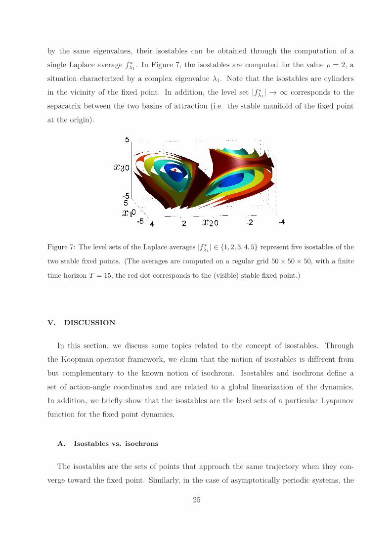
by the same eigenvalues, their isostables can be obtained through the computation of a
single Laplace average f ∗λ1
. In Figure 7, the isostables are computed for the value ρ = 2, a
situation characterized by a complex eigenvalue λ1. Note that the isostables are cylinders
in the vicinity of the fixed point. In addition, the level set |f ∗λ1
| → ∞ corresponds to the
separatrix between the two basins of attraction (i.e. the stable manifold of the fixed point
at the origin).
Figure 7: The level sets of the Laplace averages |f∗λ1
| ∈ {1, 2, 3, 4, 5} represent five isostables of the
two stable fixed points. (The averages are computed on a regular grid 50 × 50 × 50, with a finite
time horizon T = 15; the red dot corresponds to the (visible) stable fixed point.)
V. DISCUSSION
In this section, we discuss some topics related to the concept of isostables. Through
the Koopman operator framework, we claim that the notion of isostables is different from
but complementary to the known notion of isochrons. Isostables and isochrons define a
set of action-angle coordinates and are related to a global linearization of the dynamics.
In addition, we briefly show that the isostables are the level sets of a particular Lyapunov
function for the fixed point dynamics.
A. Isostables vs. isochrons
The isostables are the sets of points that approach the same trajectory when they con-
verge toward the fixed point. Similarly, in the case of asymptotically periodic systems, the
25

isochrons are the set of points that converge toward the same trajectory on the limit cycle
[32]. It follows that isostables (of fixed points) and isochrons (of limit cycles) are conceptu-
ally related. However, these two concepts are also characterized by intrinsic differences and
turn out to be complementary.
The difference between isostables and isochrons can be understood through the framework
of the Koopman operator. The isostables have been defined as the level sets of the absolute
value of the Koopman eigenfunction |s1(x)| (Section II B). In contrast, the isochrons of limit
cycles were computed in [18] by using the argument of a Koopman eigenfunction. Similarly,
the isochrons of fixed points (characterized by a complex eigenvalue λ1) can be defined as
the levels sets of the argument ∠s1(x). These sets (also called isochronous sections) are
well-known and usually defined as the sets invariant under a particular return map (i.e. the
discrete map φ(T1, ·) considered in Proposition 2). Also, their existence, which is not trivial
in the case of weak foci (i.e. purely imaginary eigenvalues) or nonsmooth vector fields, has
been investigated in [9, 28]. In the case of linear systems, the isochrons correspond to radial
lines that intersect at the fixed point (see Figure 3(b)). For nonlinear systems, they are
tangent to radial lines at the fixed point but are characterized by a more complex geometry
(see Figure 8). Note that, when they exist, the isochrons are uniquely determined by their
toplogical properties: they define the unique periodic partition of the state space (of period
T1). In contrast, more care was needed to define the isostables as the level sets of the unique
smooth eigenvalue s1.
Isostables and isochrons appear to be two different but complementary notions. On
one hand, the isostables are related to the stability property of the system and provide
information on how fast the trajectories converge toward the attractor. On the other hand,
the isochrons are related to a notion of phase and provide information on the asymptotic
behavior of the trajectories on the attractor. Given (11), the isostables are related to the
propertyd
dt|s1(φt(x))| = σ1|s1(φt(x))| (22)
while the isochrons are characterized by
d
dt∠s1(φt(x)) = ω1 . (23)
In the case of fixed points, it is clear that the isochrons are not relevant to characterize the
synchronous convergence of the trajectories, a fact that stresses the importance of considering
26

the isostables instead.
v
w
−0.2 −0.1 0 0.1 0.2
−0.2
−0.1
0
0.1
0.2
Figure 8: For a fixed point with a complex eigenvalue λ1, the isostables (black curves) and the
isochrons (red curves) of the fixed point are the level sets of |s1(x)| and ∠s1(x), respectively.
In the vicinity of the fixed point, the isostables are ellipses and the isochrons are straight lines.
(The numerical computations are performed for the FitzHugh-Nagumo model, with the parameters
considered in Section IV A 2; the blue dot represents the fixed point.)
B. Action-angle coordinates and global linearization
For a two-dimensional dynamical system which admits a spiral sink (two complex eigen-
values), the families of isostables and isochrons provide an action-angle coordinates repre-
sentation of the dynamics. More precisely, (22) and (23) imply that, with the variables
(r, θ) = (|s1(x)|,∠s1(x)), the system is characterized by the (action-angle) dynamics
r = σ1r
θ = ω1
in the basin of attraction of the fixed point. For systems of higher dimension, the action-angle
dynamics are obtained with several Koopman eigenfunctions, i.e. (rj , θj) = (|sj(x)|,∠sj(x))
leads to rj = σjrj, θj = ωj. Note that this was also shown in Section II A 2 in the case of
linear systems with a spiral sink.
When expressed in the action-angle coordinates, the dynamics become linear. This is
in agreement with the recent work [15] showing that a coordinate system which linearizes
27

the dynamics is naturally provided by the eigenfunctions of the Koopman operator (see also
Appendix A). Namely, in the new variables yj = sj(x), the system dynamics are given by
d
dt
y1
...
yn
=
λ1 0. . .
0 λ2
y1
...
yn
.
Moreover, the linear change of coordinates
z1
...
zn
= V
y1
...
yn
, (24)
where the columns of V are the eigenvectors vj of the Jacobian matrix J at the fixed point,
leads to the linear dynamics
d
dt
z1
...
zn
= J
z1
...
z2
.
For the two-dimensional FitzHugh-Nagumo model, the coordinates (z1, z2) are represented in
Figure 9 and are equivalent to the action-angle coordinates (r, θ) (Figure 8). They correspond
to Cartesian coordinates in the vicinity of the fixed point, where the linearized dynamics are
a good approximation of the nonlinear dynamics (see also (A3) in Appendix A). But owing
to the nonlinearity, the coordinates are deformed as their distance from the fixed point
increases. The comparison between these coordinates and regular Cartesian coordinates
therefore appears as a measure of the system nonlinearity.
In the case of two-dimensional systems with a stable spiral sink, the derivation of action-
angle coordinates and the global linearization are obtained through the isostables and the
isochrons, that is, with only the first Koopman eigenfunction s1(x). For higher-dimensional
systems (or two-dimensional systems with a sink node), global linearization involves several
Koopman eigenfunctions sj(x) (see [15] for a detailed study), which can be obtained through
the generalized Laplace averages (see Remark 3). In the context of model reduction, or when
the dynamics are significantly slow in one particular direction, the first eigenfunction—
related to the isostable—is however sufficient to retain the main information on the system
behavior.
28

v
w
−0.2 −0.1 0 0.1 0.2
−0.2
−0.1
0
0.1
0.2
Figure 9: The coordinates z1 (black curves) and z2 (red curves) correspond to Cartesian coordinates
in the vicinity of the fixed point but are deformed when far from the fixed point. (The numerical
computations are performed for the FitzHugh-Nagumo model, with the parameters considered in
Section IV A 2; the blue dot represents the fixed point.)
C. Lyapunov function and contracting metric
As a consequence of the linearization properties illustrated in the previous section, the
Koopman eigenfunctions—and in particular the isostables—can be used to derive Lyapunov
functions and contracting metrics for the system.
In the particular case of two-dimensional systems with a spiral sink, the isostables are the
level sets of the particular Lyapunov function V(x) = |s1(x)| (see Figure 10 for the FitzHugh-
Nagumo model). Indeed, (22) implies that V(x) = σ1V(x) < 0 ∀x ∈ B(x∗) \ {x∗} and one
verifies that V(x∗) = 0. This function is a special Lyapunov function of the system, in the
sense that its decay rate is constant everywhere. (Note that the function V = ln(|s1(x)|)/σ1
satisfies V = −1 but with V(x∗) = −∞.)
In addition, the isostables are related to a metric which is contracting in the basin of
attraction of the fixed point. Namely, the distance
d(x, x′) = |s1(x) − s1(x′)|
is well-defined and (11) implies that
d
dtd(
φt(x), φt(x′))
= σ1d(x, x′) < 0 , ∀x 6= x′ ∈ B(x∗) .
For more general systems that admit a stable fixed point, the function V(x) = |s1(x)| is still
decreasing along the trajectories, but V(x) = 0 does not imply x = x∗ (V is zero on the
29

Figure 10: The function V = |s1(x)| is a particular Lyapunov function for the system (here, the
FitzHugh-Nagumo model with the parameters considered in Section IV A 2). One verifies that
the function decreases with a constant rate along a trajectory (black curve). Note also that the
unstable slow manifold (region v < 0, w ≈ 0) is characterized by a line of maxima of the Lyapunov
function.
whole isostable Iτ=∞ that contains the fixed point). However, the function can be used with
the LaSalle invariance principle. To obtain a good Lyapunov function, several Koopman
eigenfunctions must be considered. For instance, the function
V(x) =
n∑
j=1
|sj(x)|p
1/p
,
with the integer p ≥ 1, satisfies
V(x) =
n∑
j=1
|sj(x)|p
1p
−1n∑
j=1
σj |sj(x)|p ≤ σ1V(x)
and V(x) = 0 iff x = x∗. In addition, a contracting metric is given by
d(
x, x′)
=
n∑
j=1
|sj(x) − sj(x′)|p
1/p
and one hasd
dtd(
φt(x), φt(x′))
≤ σ1d(x, x′) , ∀x, x′ ∈ B(x∗) .
It follows from the above observations that showing the existence of stable eigenfunctions of
the Koopman operator is sufficient to prove the global stability of the attractor. Therefore,
30

the Koopman operator framework could potentially yield an alternative method for the
global stability analysis of nonlinear systems.
VI. CONCLUSION
In this paper, the well-known phase reduction of asymptotically periodic systems has
been extended to the class of systems which admit a stable fixed point. In the context
of the Koopman operator framework, the approach is not restricted to excitable systems
with slow-fast dynamics but is valid in more general situations. The isostables required for
the reduction of the dynamics, which correspond is some cases to the fibers of a particular
invariant manifold of the system, are interpreted as the level sets of an eigenfunction of the
Koopman operator. In addition, they are shown to be different from the concept of isochrons
that prevails for asymptotically periodic systems. Beyond its theoretical implications, the
framework also yields an efficient (forward integration) method for computing the isostables,
which is based on the estimation of Laplace averages along the trajectories.
The reduction of the dynamics through the Koopman operator framework leads to an
action-angle coordinates representation that is intimately related to a global linearization
of the system. More precisely, the proposed reduction procedure is nothing but a global
linearization of the system where only one direction of interest is considered, which retains
the main information on the system behavior (i.e. the slowest direction). In this context,
the isostables—related to the action—or the isochrons—related to the angle— used for the
reduction are particular objects involved in the global linearization process. Given this
relation between reduction methods and linearization, research perspectives are twofold.
On the one hand, convenient Laplace average methods could be developed for linearization
purposes (e.g. computation of the isostables of limit cycles [11] in the whole—possibly
high-dimensional—basin of attraction), and for the computation of (un)stable manifolds as
well. On the other hand, the Koopman operator framework can be further exploited for the
reduction of more general dynamical systems (e.g. chaotic systems).
31

Acknowledgments
The work was completed while A. Mauroy held a postdoctoral fellowship from the Belgian
American Educational Foundation and was partially funded by Army Research Office Grant
W911NF-11-1-0511, with Program Manager Dr. Sam Stanton.
Appendix A: SPECTRAL DECOMPOSITION OF THE KOOPMAN OPERATOR
In this appendix, we derive the expansion (10) of an observable onto the eigenfunctions of
the Koopman operator. Consider the change of variable s : x 7→ y, with yj = sj(x), where
sj is an eigenfunction of the Koopman operator. It follows that s(x∗) = 0 and, given (11),
the dynamics is linearized in the y variable, i.e. yj = λj yj. According to the linearization
Poincare theorem [8], the transformation s is analytic since the vector field F is analytic and
the eigenvalues are nonresonant (and provided there is no unstable fixed point in B(x∗)). If
an observable f is analytic, the Taylor expansion of f(s−1(y)) around the origin yields
f(s−1(y)) = f(x∗) + ∇fT (x∗) Js−1y +1
2yT JT
s−1HJs−1 y +1
2yT
n∑
k=1
∂f
∂xk
∣
∣
∣
∣
∣
x∗
Hs−1k
y + h.o.t. ,
(A1)
where Js−1 is the Jacobian matrix of s−1 at the origin (i.e. Js−1,ij = ∂s−1i /∂yj(0)), H is
the Hessian matrix of f at x∗ (i.e. Hij = ∂2f/(∂xi∂xj)(x∗)), and Hs−1
kis the Hessian
matrix of s−1k at the origin (i.e. Hs−1
k,ij = ∂2s−1
k /(∂yi∂yj)(0)). Using the relationship y =
(s1(x), . . . , sn(x)), we can turn the expansion (A1) into an expansion of f onto the products
of the eigenfunctions sj . For a vector-valued observable f , we obtain
f(x) =∑
{k1,...,kn}∈Nn
vk1···knsk1
1 (x) · · · skn
n (x) (A2)
with the (first) Koopman modes
vk1···kn=
f(x∗) kj = 0 ∀j ,n∑
k=1
∂f
∂xk
∣
∣
∣
∣
∣
x∗
∂s−1k
∂yj
∣
∣
∣
∣
∣
0
kj = 1 , ki = 0 ∀i 6= j ,
n∑
k=1
n∑
l=1
∂2f
∂xk∂xl
∣
∣
∣
∣
∣
x∗
∂s−1k
∂yi
∣
∣
∣
∣
∣
0
∂s−1l
∂yj
∣
∣
∣
∣
∣
0
+n∑
k=1
∂f
∂xk
∣
∣
∣
∣
∣
x∗
∂2s−1k
∂yi∂yj
∣
∣
∣
∣
∣
0
ki = kj = 1 , kr = 0 ∀r 6= {i, j} ,
1
2
n∑
k=1
n∑
l=1
∂2f
∂xk∂xl
∣
∣
∣
∣
∣
x∗
∂s−1k
∂yi
∣
∣
∣
∣
∣
0
∂s−1l
∂yi
∣
∣
∣
∣
∣
0
+1
2
n∑
k=1
∂f
∂xk
∣
∣
∣
∣
∣
x∗
∂2s−1k
∂y2i
∣
∣
∣
∣
∣
0
ki = 2 , kj = 0 ∀j 6= i .
32

The other (higher-order) Koopman modes can be derived similarly from (A1). Since the
eigenfunctions satisfy (11), the relationship (10) directly follows from (A2).
For the observable f(x) = x, the Koopman modes are given by
vk1···kn=
1
k1! . . . kn!
∂k1···kns−1
∂k1y1 · · · ∂knyn
∣
∣
∣
∣
∣
0
.
In particular, the eigenvectors of the Jacobian matrix J of F (i.e. vj = vk1···kn, with kj = 1,
ki = 0 ∀i 6= j) correspond to
vj =∂s−1
∂yj
∣
∣
∣
∣
∣
0
and one has Js−1 = V, where the columns of V are the eigenvectors vj. It follows that the
variables z introduced in (24) satisfy z = Js−1y so that (A1) implies
x = x∗ + z + o(‖z‖) . (A3)
In addition, the derivation of y = s(s−1(y)) at the origin leads to
δij =
⟨
∇si(x∗),
∂s−1
∂yj
∣
∣
∣
∣
∣
c
0
⟩
=⟨
∇si(x∗), vc
j
⟩
.
Therefore, the gradient ∇si(x∗) is the left eigenvector vc
i of J (associated with the eigenvalue
λi) and one has
si(x) = 〈x − x∗, ∇sci(x
∗)〉 + o(‖x − x∗‖) = 〈x − x∗, vi〉 + o(‖x − x∗‖) , (A4)
which implies that, for ‖x − x∗‖ ≪ 1, the eigenfunction si(x) is well approximated by the
eigenfunction of the linearized system.
[1] V. Arnold, Mathematical methods of classical mechanics, vol. 60, Springer, 1989.
[2] E. Brown, J. Moehlis, and P. Holmes, On the phase reduction and response dynamics
of neural oscillator populations, Neural Computation, 16 (2004), pp. 673–715.
[3] S. Coombes and A. Osbaldestin, Period-adding bifurcations and chaos in a periodically
stimulated excitable neural relaxation oscillator, Physical Review E, 62 (2000), p. 4057.
[4] S. M. Cox and A. J. Roberts, Initial conditions for models of dynamical systems, Physica
D: Nonlinear Phenomena, 85 (1995), pp. 126–141.
33

[5] N. Fenichel, Persistence and smoothness of invariant manifolds for flows, Indiana Univ.
Math. J, 21 (1971), p. 1972.
[6] , Asymptotic stability with rate conditions, Indiana Univ. Math. J, 23 (1973), p. 74.
[7] R. FitzHugh, Impulses and physiological states in models of nerve membrane, Biophysical
Journal, 1 (1961), pp. 445–466.
[8] P. Gaspard, G. Nicolis, A. Provata, and S. Tasaki, Spectral signature of the pitchfork
bifurcation: Liouville equation approach, Physical Review E, 51 (1995), p. 74.
[9] J. Gine and M. Grau, Characterization of isochronous foci for planar analytic differential
systems, in Proceedings of the Royal Society of Edinburgh-A-Mathematics, vol. 135, Cam-
bridge Univ Press, 2005, pp. 985–998.
[10] J. Guckenheimer, Isochrons and phaseless sets, Journal of Mathematical Biology, 1 (1975),
pp. 259–273.
[11] A. Guillamon and G. Huguet, A computational and geometric approach to phase resetting
curves and surfaces, SIAM Journal On Applied Dynamical Systems, 8 (2009), pp. 1005–1042.
[12] M. W. Hirsch, C. C. Pugh, and M. Shub, Invariant manifolds, vol. 583 of Lecture Notes
in Mathematics, Springler-Verlag, 1977.
[13] N. Ichinose, K. Aihara, and K. Judd, Extending the concept of isochrons from oscillatory
to excitable systems for modeling an excitable neuron, International Journal of Bifurcation and
Chaos, 8 (1998), pp. 2375–2385.
[14] E. M. Izhikevich, Dynamical Systems in Neuroscience: The Geometry of Excitability and
Bursting, MIT press, 2007.
[15] Y. Lan and I. Mezic, Linearization in the large of nonlinear systems and Koopman operator
spectrum, Physica D, 242 (2013), pp. 42–53.
[16] I. G. Malkin, The methods of Lyapunov and Poincare in the theory of nonlinear oscillations,
Gostekhizdat, Moscow-Leningrad, (1949).
[17] N. Masuda and K. Aihara, Synchronization of pulse-coupled excitable neurons, Physical
Review E, 64 (2001), pp. 051906/1–13.
[18] A. Mauroy and I. Mezic, On the use of Fourier averages to compute the global isochrons
of (quasi)periodic dynamics, Chaos, 22 (2012), p. 033112.
[19] I. Mezic, Spectral properties of dynamical systems, model reduction and decompositions, Non-
linear Dynamics, 41 (2005), pp. 309–325.
34

[20] , Analysis of fluid flows via spectral properties of Koopman operator, Annual Review of
Fluid Mechanics, 45 (2013).
[21] I. Mezic and A. Banaszuk, Comparison of systems with complex behavior, Physica D-
Nonlinear Phenomena, 197 (2004), pp. 101–133.
[22] J. Nagumo, S. Arimoto, and S. Yoshizawa, An active pulse transmission line simulating
nerve axon, in Proceedings of the IRE, vol. 50, 1962, pp. 2061–2070.
[23] H. M. Osinga and J. Moehlis, Continuation-based computation of global isochrons, SIAM
Journal on Applied Dynamical Systems, 9 (2010), pp. 1201–1228.
[24] A. Rabinovitch and I. Rogachevskii, Threshold, excitability and isochrones in the
Bonhoeffer–van der Pol system, Chaos, 9 (1999), pp. 880–886.
[25] A. Rabinovitch, R. Thieberger, and M. Friedman, Forced Bonhoeffer-van der Pol
oscillator in its excited mode, Physical Review E, 50 (1994), pp. 1572–1578.
[26] A. J. Roberts, Appropriate initial conditions for asymptotic descriptions of the long term
evolution of dynamical systems, Australian Mathematical Society, Journal, Series B-Applied
Mathematics, 31 (1989), pp. 48–75.
[27] C. W. Rowley, I. Mezic, S. Bagheri, P. Schlatter, and D. S. Henningson, Spectral
analysis of nonlinear flows, Journal of Fluid Mechanics, 641 (2009), pp. 115–127.
[28] M. Sabatini, Non-periodic isochronous oscillations in plane differential systems, Annali di
Matematica Pura ed Applicata, 182 (2003), pp. 487–501.
[29] K. Shaw, Y. Park, H. Chiel, and P. Thomas, Phase resetting in an asymptotically
phaseless system: On the phase response of limit cycles verging on a heteroclinic orbit, SIAM
Journal on Applied Dynamical Systems, 11 (2012), pp. 350–391.
[30] L. Trotta, E. Bullinger, and R. Sepulchre, Global analysis of dynamical decision-
making models through local computation around the hidden saddle, PloS ONE, 7 (2012),
p. e33110.
[31] A. Winfree, The Geometry of Biological Time, New York: Springler-Verlag, 2001 (Second
Edition).
[32] A. T. Winfree, Patterns of phase compromise in biological cycles, Journal of Mathematical
Biology, 1 (1974), pp. 73–95.
35