ISOLDE ADLER, MAMADOU MOUSTAPHA KANT´E, AND O-JOUNG …
28
arXiv:1403.1081v3 [math.CO] 21 Aug 2015 LINEAR RANK-WIDTH OF DISTANCE-HEREDITARY GRAPHS I. A POLYNOMIAL-TIME ALGORITHM ISOLDE ADLER, MAMADOU MOUSTAPHA KANT ´ E, AND O-JOUNG KWON Abstract. Linear rank-width is a linearized variation of rank-width, and it is deeply related to matroid path-width. In this paper, we show that the linear rank-width of every n-vertex distance-hereditary graph, equivalently a graph of rank-width at most 1, can be computed in time Opn 2 ¨ log 2 nq, and a linear layout witnessing the linear rank-width can be computed with the same time complexity. As a corollary, we show that the path-width of every n-element matroid of branch-width at most 2 can be computed in time Opn 2 ¨ log 2 nq, provided that the matroid is given by an independent set oracle. To establish this result, we present a characterization of the linear rank- width of distance-hereditary graphs in terms of their canonical split decom- positions. This characterization is similar to the known characterization of the path-width of forests given by Ellis, Sudborough, and Turner [The vertex separation and search number of a graph. Inf. Comput., 113(1):50–79, 1994]. However, different from forests, it is non-trivial to relate substructures of the canonical split decomposition of a graph with some substructures of the given graph. We introduce a notion of ‘limbs’ of canonical split decompositions, which correspond to certain vertex-minors of the original graph, for the right characterization. 1. Introduction Rank-width [26] is a graph parameter introduced by Oum and Seymour with the goal of efficient approximation of the clique-width [7] of a graph. Linear rank-width can be seen as the linearized variant of rank-width, and it is similar to path-width, which can be seen as the linearized variant of tree-width. While path-width is a well-studied notion, much less is known about linear rank-width. Vertex-minor is a graph containment relation where rank-width and linear rank-width do not increase when taking this operation. Rank-width is related to matroid branch-width, which has an important role in structural theory on matroids. We refer to the series of papers by Geelen, Gerards, and Whittle on the Matroid Minors Project [15, 17] and Rota’s Conjecture [18] for more information on matroid branch-width. It is known that the matroid branch- width (matroid path-width) of a binary matroid is equal to the rank-width (linear rank-width) of its fundamental graph plus one [25]. This equality can be further generalized to matroids over a fixed finite field with the finite field version of rank- width [20, 21]. Hence new results on (linear) rank-width will immediately yield new results on matroid branch-width or on matroid path-width. In this paper, we will derive a complexity result for computing matroid path-width from linear rank-width. Kashyap [22] showed that it is NP-hard to compute matroid path-width on binary matroids. By reducing from matroid path-width, we can show that computing linear The first author is supported by the German Research Council, Project GalA, AD 411/1-1. The third author was partially supported by Basic Science Research Program through the Na- tional Research Foundation of Korea (NRF) funded by the Ministry of Science, ICT & Future Planning (2011-0011653) while the author was at Korea Advanced Institute of Science and Tech- nology, and was also partially supported by ERC Starting Grant PARAMTIGHT (No. 280152). A preliminary version appeared in the proceedings of WG’14. 1
Transcript of ISOLDE ADLER, MAMADOU MOUSTAPHA KANT´E, AND O-JOUNG …
arX
iv:1
403.
1081
v3 [
mat
h.C
O]
21
Aug
201
5
LINEAR RANK-WIDTH OF DISTANCE-HEREDITARY GRAPHS
I. A POLYNOMIAL-TIME ALGORITHM
ISOLDE ADLER, MAMADOU MOUSTAPHA KANTE, AND O-JOUNG KWON
Abstract. Linear rank-width is a linearized variation of rank-width, and it isdeeply related to matroid path-width. In this paper, we show that the linearrank-width of every n-vertex distance-hereditary graph, equivalently a graphof rank-width at most 1, can be computed in time Opn2 ¨ log
2nq, and a linear
layout witnessing the linear rank-width can be computed with the same timecomplexity. As a corollary, we show that the path-width of every n-elementmatroid of branch-width at most 2 can be computed in time Opn2 ¨ log
2nq,
provided that the matroid is given by an independent set oracle.
To establish this result, we present a characterization of the linear rank-width of distance-hereditary graphs in terms of their canonical split decom-positions. This characterization is similar to the known characterization ofthe path-width of forests given by Ellis, Sudborough, and Turner [The vertexseparation and search number of a graph. Inf. Comput., 113(1):50–79, 1994].However, different from forests, it is non-trivial to relate substructures of thecanonical split decomposition of a graph with some substructures of the givengraph. We introduce a notion of ‘limbs’ of canonical split decompositions,which correspond to certain vertex-minors of the original graph, for the rightcharacterization.
1. Introduction
Rank-width [26] is a graph parameter introduced by Oum and Seymour with thegoal of efficient approximation of the clique-width [7] of a graph. Linear rank-widthcan be seen as the linearized variant of rank-width, and it is similar to path-width,which can be seen as the linearized variant of tree-width. While path-width is awell-studied notion, much less is known about linear rank-width. Vertex-minor is agraph containment relation where rank-width and linear rank-width do not increasewhen taking this operation.
Rank-width is related to matroid branch-width, which has an important role instructural theory on matroids. We refer to the series of papers by Geelen, Gerards,and Whittle on the Matroid Minors Project [15, 17] and Rota’s Conjecture [18] formore information on matroid branch-width. It is known that the matroid branch-width (matroid path-width) of a binary matroid is equal to the rank-width (linearrank-width) of its fundamental graph plus one [25]. This equality can be furthergeneralized to matroids over a fixed finite field with the finite field version of rank-width [20, 21]. Hence new results on (linear) rank-width will immediately yieldnew results on matroid branch-width or on matroid path-width. In this paper,we will derive a complexity result for computing matroid path-width from linearrank-width.
Kashyap [22] showed that it is NP-hard to compute matroid path-width on binarymatroids. By reducing from matroid path-width, we can show that computing linear
The first author is supported by the German Research Council, Project GalA, AD 411/1-1.The third author was partially supported by Basic Science Research Program through the Na-
tional Research Foundation of Korea (NRF) funded by the Ministry of Science, ICT & FuturePlanning (2011-0011653) while the author was at Korea Advanced Institute of Science and Tech-nology, and was also partially supported by ERC Starting Grant PARAMTIGHT (No. 280152).A preliminary version appeared in the proceedings of WG’14.
1

2 I. ADLER, M.M. KANTE, AND O. KWON
rank-width is NP-hard in general. Therefore it is natural to ask which graph classesallow for an efficient computation. Until now, the only known non-trivial result is forforests [1]. Our main result is that distance-hereditary graphs allow a polynomial-time algorithm to compute linear rank-width. A graph G is distance-hereditary,if for every pair of two vertices u and v of G, the distance between u and v inany connected induced subgraph of G containing both u and v, is the same as thedistance between u and v in G. Distance-hereditary graphs are exactly graphs ofrank-width at most 1 [25], and include all forests and cographs.
Theorem 6.1. The linear rank-width of every n-vertex distance-hereditary graphcan be computed in time Opn2 ¨ log2 nq. Moreover, a linear layout of the graphwitnessing the linear rank-width can be computed with the same time complexity.
In contrast, computing the path-width of distance-hereditary graphs is known tobe NP-hard [23]. Bodlaender and Kloks [5] showed that it is possible to compute thepath-width of graphs of bounded tree-width in polynomial time. The correspond-ing question for rank-width is still open: Is there a polynomial-time algorithm tocompute the linear rank-width of graphs of rank-width at most ℓ (for fixed ℓ)?Since distance-hereditary graphs are exactly the graphs of rank-width at most 1,Theorem 6.1 is a first step towards an answer of this question.
A direct consequence of Theorem 6.1 is the possibility to compute the path-widthof matroids with branch-width at most 2 in polynomial time.
Corollary 7.4. The path-width of every n-element matroid of branch-width at most2 can be computed in time Opn2 ¨ log2 nq, provided that the matroid is given by anindependent set oracle. Moreover, a linear layout of the matroid witnessing thepath-width can be computed with the same time complexity.
The main ingredient of our algorithm is a new characterization of the linear rank-width of distance-hereditary graphs (Theorem 4.1). Our characterization makes useof the special structure of canonical split decompositions [8] of distance-hereditarygraphs. Roughly, a canonical split decomposition decomposes a distance-hereditarygraph in a tree-like fashion into complete graphs and stars, and our characterizationis recursive along the sub-decompositions of the split decomposition.
While a similar idea has been exploited in [1, 12, 24] for other parameters, herewe encounter a new problem. When we take a subgraph of a given split decom-position, the obtained split decomposition may have vertices that do not representvertices of the original graph. It is not at all obvious how to deal with these verticesin the recursive step. We handle this by introducing limbs of canonical split de-compositions, that correspond to certain vertex-minors of the original graphs, andhave the desired properties to allow our characterization. We think that the notionof limbs may be useful in other contexts, too, and hopefully, it can be extended toother graph classes and allow for further new efficient algorithms.
The paper is structured as follows. Section 2 introduces the basic notions, inparticular linear rank-width, vertex-minors, and split decompositions. In Section 3,we define limbs and its canonical decompositions, called canonical limbs, and showsome basic properties. We use them in Section 4 for our characterization of thelinear rank-width of distance-hereditary graphs. In Section 5, we establish essentialproperties of canonical limbs, which will be used to obtain the running time ofour algorithm. Section 6 presents the Opn2 ¨ log2 nq-time algorithm for computingthe linear rank-width of distance-hereditary graphs, and in Section 7, we obtainan algorithm for computing the path-width of matroids of branch-width at most 2as a corollary. To obtain the running time, we need the fact that every n-vertexdistance-hereditary graph G has linear rank-width at most log2 n. We prove it inSection 8.

LRW OF DH GRAPHS I: A POLYNOMIAL-TIME ALGORITHM 3
2. Preliminaries
In this paper, graphs are finite, simple and undirected, unless stated otherwise.Our graph terminology is standard, see for instance [11]. Let G be a graph. Wedenote the vertex set of G by V pGq and the edge set by EpGq. An edge betweenx and y is written xy (equivalently yx). For X Ď V pGq, we denote by GrXs thesubgraph of G induced by X , and let GzX :“ GrV pGqzXs. For shortcut we writeGzx for Gztxu. For a vertex x of G, let NGpxq be the set of neighbors of x in G
and we call |NGpxq| the degree of x in G. An edge e of G is called a cut-edge if itsremoval increases the number of connected components of G.
A tree is a connected acyclic graph. A leaf of a tree is a vertex of degree one.A path is a tree where every vertex has degree at most two. The length of a pathis the number of its edges. A star is a tree with a distinguished vertex, called itscenter, adjacent to all other vertices. A complete graph is a graph with all possibleedges. A graph G is called distance-hereditary if for every pair of two vertices x andy of G the distance of x and y in G equals the distance of x and y in any connectedinduced subgraph containing both x and y [3].
2.1. Linear rank-width and vertex-minors. For setsR and C, an pR,Cq-matrixis a matrix whose rows and columns are indexed by R and C, respectively. For anpR,Cq-matrix M , X Ď R, and Y Ď C, let M rX,Y s be the submatrix of M whoserows and columns are indexed by X and Y , respectively.
Linear rank-width. Let G be a graph. We denote by AG the adjacency matrix ofG over the binary field. The cut-rank function of G is a function cutrkG : 2V pGq Ñ Z
where for each X Ď V pGq,
cutrkGpXq :“ rankpAGrX,V pGqzXsq.
A sequence px1, . . . , xnq of the vertex set V pGq is called a linear layout of G. If|V pGq| ě 2, then the width of a linear layout px1, . . . , xnq of G is defined as
max1ďiďn´1
tcutrkGptx1, . . . , xiuqu.
The linear rank-width of G, denoted by lrwpGq, is defined as the minimum widthover all linear layouts of G if |V pGq| ě 2, and otherwise, let lrwpGq :“ 0.
Caterpillars and complete graphs have linear rank-width at most 1. Ganian [13]gave a characterization of the graphs of linear rank-width at most 1, and call themthread graphs. Adler and Kante [1] showed that linear rank-width and path-widthcoincide on forests, and therefore, there is a linear time algorithm to compute thelinear rank-width of forests. It is easy to see that the linear rank-width of a graphis the maximum over the linear rank-widths of its connected components.
To obtain the bound presented in Theorem 6.1, we will need the fact that thelinear rank-width of an n-vertex distance-hereditary graph G is at most log2 n. Infact, we generally show that the linear rank-width of a graph with rank-width k isat most ktlog2 nu. The proof scheme is similar to the one for path-width [4].
A tree is subcubic if it has at least two vertices and every inner vertex hasdegree 3. A rank-decomposition of a graph G is a pair pT, Lq, where T is a subcubictree and L is a bijection from the vertices of G to the leaves of T . For an edgee in T , T ze induces a partition pXe, Yeq of the leaves of T . The width of an edgee is defined as cutrkGpL´1pXeqq. The width of a rank-decomposition pT, Lq is themaximum width over all edges of T . The rank-width of G, denoted by rwpGq, is theminimum width over all rank-decompositions of G. If |V pGq| ď 1, then G admitsno rank-decomposition and rwpGq “ 0.
Theorem 2.1 (Oum [25]). A graph is distance-hereditary if and only if it hasrank-width at most 1.

4 I. ADLER, M.M. KANTE, AND O. KWON
a b b a
Figure 1. Pivoting an edge ab.
Lemma 2.2. Let k be a positive integer and let G be a graph of rank-width k. ThenlrwpGq ď ktlog2|V pGq|u.
Lemma 2.2 will be proved in Section 8.
Vertex-minors. For a graph G and a vertex x of G, the local complementation atx of G is an operation to replace the subgraph induced by the neighbors of x withits complement. The resulting graph is denoted by G ˚ x. If H can be obtainedfrom G by applying a sequence of local complementations, then G and H are calledlocally equivalent. A graph H is called a vertex-minor of a graph G if H can beobtained from G by applying a sequence of local complementations and deletionsof vertices.
Lemma 2.3 (Oum [25]). Let G be a graph and let x be a vertex of G. Then forevery subset X of V pGq, we have cutrkGpXq “ cutrkG˚xpXq. Therefore, everyvertex-minor H of G satisfies that lrwpHq ď lrwpGq.
For an edge xy of G, let W1 :“ NGpxq X NGpyq, W2 :“ pNGpxqzNGpyqqztyu,and W3 :“ pNGpyqzNGpxqqztxu. The pivoting on xy of G, denoted by G ^ xy, isthe operation to complement the adjacencies between distinct sets Wi and Wj , andswap the vertices x and y. It is known that G ^ xy “ G ˚ x ˚ y ˚ x “ G ˚ y ˚ x ˚ y
[25]. See Figure 1 for an example.We introduce some basic lemmas on local complementations, which will be used
in several places.
Lemma 2.4. Let G be a graph and x, y P V pGq such that xy R EpGq. ThenG ˚ x ˚ y “ G ˚ y ˚ x.
Proof. It is straightforward as applying a local complementation at x or y does notchange the neighbor sets of x and y. �
Lemma 2.5. Let G be a graph and x, y, z P V pGq such that xy, xz R EpGq andyz P EpGq. Then G ˚ x ^ yz “ G ^ yz ˚ x.
Proof. By the definition of pivoting, G ˚ x ^ yz “ G ˚ x ˚ y ˚ z ˚ y. Note thatxy R EpGq, xz R EpG ˚ yq, and xy R EpG ˚ y ˚ zq. Therefore, by Lemma 2.4,G˚x˚y˚z˚y “ pG˚yq˚x˚z˚y “ pG˚y˚zq˚x˚y “ pG˚y˚z˚yq˚x “ G^yz˚x. �
Lemma 2.6 (Oum [25]). Let G be a graph and x, y, z P V pGq such that xy, yz PEpGq. Then G ^ xy ^ xz “ G ^ yz.
2.2. Split decompositions and local complementations. We will follow thedefinition of split decompositions in [6]. We notice that split decompositions areusually defined on connected graphs. For computing the linear rank-width of adistance-hereditary graph, it is enough to compute the linear rank-width of its con-nected components and take the maximum over all those values. Thus we willmostly assume that the given graph is connected in this paper, and use split de-compositions in usual sense.

LRW OF DH GRAPHS I: A POLYNOMIAL-TIME ALGORITHM 5
Let G be a connected graph. A split in G is a vertex partition pX,Y q of G suchthat |X |, |Y | ě 2 and rankpAGrX,Y sq “ 1. In other words, pX,Y q is a split inG if |X |, |Y | ě 2 and there exist non-empty sets X 1 Ď X and Y 1 Ď Y such thattxy P EpGq | x P X, y P Y u “ txy | x P X 1, y P Y 1u. Notice that not all connectedgraphs have a split, and those that do not have a split are called prime graphs.
A marked graph D is a connected graph D with a set of edges MpDq, calledmarked edges, that form a matching such that every edge in MpDq is a cut-edge.The ends of the marked edges are called marked vertices, and the components ofpV pDq, EpDqzMpDqq are called bags of D. The edges in EpDqzMpDq are calledunmarked edges, and the vertices that are not marked vertices are called unmarkedvertices. If pX,Y q is a split in G, then we construct a marked graph D that consistsof the vertex set V pGq Y tx1, y1u for two distinct new vertices x1, y1 R V pGq and theedge set EpGrXsq Y EpGrY sq Y tx1y1u Y E1 where we define x1y1 as marked and
E1 :“ tx1x | x P X and there exists y P Y such that xy P EpGquY
ty1y | y P Y and there exists x P X such that xy P EpGqu.
The marked graph D is called a simple decomposition of G.A split decomposition of a connected graph G is a marked graph D defined in-
ductively to be either G or a marked graph defined from a split decomposition D1
of G by replacing a component H of pV pD1q, EpD1qzMpD1qq with a simple decom-position of H . For a marked edge xy in a split decomposition D, the recompositionof D along xy is the split decomposition D1 :“ pD ^ xyqztx, yu. For a split decom-position D, let GrDs denote the graph obtained from D by recomposing all markededges. Note that if D is a split decomposition of G, then GrDs “ G. Since eachmarked edge of a split decomposition D is a cut-edge and all marked edges form amatching, if we contract all unmarked edges in D, then we obtain a tree. We call itthe decomposition tree of G associated with D and denote it by TD. To distinguishthe vertices of TD from the vertices of G or D, the vertices of TD will be callednodes. Obviously, the nodes of TD are in bijection with the bags of D. Two bagsof D are called neighbor bags if their corresponding nodes in TD are adjacent.
A split decomposition D of G is called a canonical split decomposition (or canon-ical decomposition for short) if each bag of D is either a prime, a star, or a completegraph, and D is not the refinement of a decomposition with the same property. Thefollowing is due to Cunningham and Edmonds [8], and Dahlhaus [9].
Theorem 2.7 (Cunningham and Edmonds [8]; Dahlhaus [9]). Every connectedgraph G has a unique canonical decomposition, up to isomorphism, and it can becomputed in time Op|V pGq| ` |EpGq|q.
From Theorem 2.7, we can talk about only one canonical decomposition of aconnected graph G because all canonical decompositions of G are isomorphic.
Let D be a split decomposition of a connected graph G with bags that are eitherprimes, complete graphs or stars (it is not necessarily a canonical decomposition).The type of a bag of D is either P , K, or S depending on whether it is a prime, acomplete graph, or a star. The type of a marked edge uv is AB where A and B arethe types of the bags containing u and v respectively. If A “ S or B “ S, then wecan replace S by Sp or Sc depending on whether the end of the marked edge is aleaf or the center of the star.
Theorem 2.8 (Bouchet [6]). Let D be a split decomposition of a connected graphwith bags that are either primes, complete graphs, or stars. Then D is a canonicaldecomposition if and only if it has no marked edge of type KK or SpSc.
We will use the following characterization of distance-hereditary graphs.
Theorem 2.9 (Bocuhet [6]). A connected graph is distance-hereditary if and onlyif each bag of its canonical decomposition is of type K or S.

6 I. ADLER, M.M. KANTE, AND O. KWON
We now relate the split decompositions of a graph and the ones of its locallyequivalent graphs. Let D be a split decomposition of a connected graph. A vertexv of D represents an unmarked vertex x (or is a representative of x) if either v “ x
or there is a path of even length from v to x in D starting with a marked edgesuch that marked edges and unmarked edges appear alternately in the path. Twounmarked vertices x and y are linked in D if there is a path from x to y in D suchthat unmarked edges and marked edges appear alternately in the path.
Lemma 2.10. Let D be a split decomposition of a connected graph. Let v1 and w1
be two vertices in a same bag of D, and let v and w be two unmarked vertices of Drepresented by v1 and w1, respectively. The following are equivalent.
(1) v and w are linked in D.(2) vw P EpGrDsq.(3) v1w1 P EpDq.
Proof. It is not hard to show that v1 and w1 are adjacent in D if and only if thereis an alternating path from v to w in D from the definition of representativity.Note that recomposing a marked edge in a split decomposition does not change theproperty that two unmarked vertices are linked, and the adjacency of two verticesin GrDs. It implies that v and w are linked in D if and only if vw P EpGrDsq. �
A local complementation at an unmarked vertex x in a split decomposition D,denoted by D˚x, is the operation to replace each bag B containing a representativew of x with B ˚ w. Observe that D ˚ x is a split decomposition of GrDs ˚ x, andMpDq “ MpD ˚ xq. Two split decompositions D and D1 are locally equivalent ifD can be obtained from D1 by applying a sequence of local complementations atunmarked vertices.
Lemma 2.11 (Bouchet [6]). Let D be the canonical decomposition of a connectedgraph. If x is an unmarked vertex of D, then D ˚ x is the canonical decompositionof GrDs ˚ x.
Remark. If D is a canonical decomposition and D1 “ D ˚ x for some unmarkedvertex v of D, then TD1 and TD are isomorphic because MpDq “ MpD1q. Thus, forevery node v of TD associated with a bag B of D, its corresponding node v1 in TD1
is associated in D1 with either
(1) B if x has no representative in B, or(2) B ˚ w if B has a representative w of v.
For easier arguments in several places, if TD is given for D, then we assume thatTD1 “ TD for every split decomposition D1 locally equivalent to D. For a canonicaldecomposition D and a node v of its decomposition tree, we write bDpvq to denotethe bag of D with which it is in correspondence.
Let x and y be linked unmarked vertices in a split decomposition D, and let Pbe the alternating path in D linking x and y. Observe that each bag contains atmost one unmarked edge in P . Notice also that if B is a bag of type S containingan unmarked edge of P , then the center of B is a representative of either x or y.The pivoting on xy of D, denoted by D^xy, is the split decomposition obtained asfollows: for each bag B containing an unmarked edge of P , if v, w P V pBq representrespectively x and y in D, then we replace B with B ^ vw. (It is worth noticingthat by Lemma 2.10, we have vw P EpBq, hence B ^ vw is well-defined.)
Lemma 2.12. Let D be a split decomposition of a connected graph. If xy PEpGrDsq, then D ^ xy “ D ˚ x ˚ y ˚ x.
Proof. Since xy P EpGrDsq, by Lemma 2.10, x and y are linked in D. It is easy tosee that by the operation D ˚ x ˚ y ˚ x, only the bags in the path from x to y are

LRW OF DH GRAPHS I: A POLYNOMIAL-TIME ALGORITHM 7
D
v w
D ˚ v
v w
D ˚ v ˚ w
v w
D ˚ v ˚ w ˚ v
v w
Figure 2. The split decomposition D˚v ˚w˚v, which is the sameas D ^ vw.
modified, and they are modified according to the definition of D^xy. See Figure 2for an example of this procedure. �
As a corollary of Lemmas 2.11 and 2.12, we get the following.
Corollary 2.13. Let D be the canonical decomposition of a connected graph. Ifxy P EpGrDsq, then D ^ xy is the canonical decomposition of GrDs ^ xy.
The following are split decomposition versions of Lemma 2.4, 2.5, 2.6, and theycan be easily verified in a same way.
Lemma 2.14. Let D be the canonical decomposition of a connected graph. Thefollowing are satisfied.
(1) If x, y are unmarked vertices of D that are not linked, then D˚x˚y “ D˚y˚x.(2) If x, y, z are unmarked vertices of D such that x is linked to neither y nor
z, and y and z are linked, then D ˚ x ^ yz “ D ^ yz ˚ x.(3) If x, y, z are unmarked vertices of D such that y is linked to both x and z,
then D ^ xy ^ xz “ D ^ yz.
For a bag B of D and a component T of DzV pBq, let us denote by ζbpD,B, T qand ζtpD,B, T q the adjacent marked vertices of D that are in V pBq and in V pT qrespectively. Observe that ζtpD,B, T q is not incident with any marked edge inT . So, when we take a sub-decomposition T from D, we regard ζtpD,B, T q as anunmarked vertex of T .
3. Limbs in canonical decompositions
We define the notion of limb that is the key ingredient in our characteriza-tion. Intuitively, a limb of a canonical decomposition is a modification of its sub-decomposition satisfying the property that if two canonical decompositions D andD1 are locally equivalent, then the limbs obtained from D and D1 on the same ver-tex set are again locally equivalent. This property allows us to characterize linear

8 I. ADLER, M.M. KANTE, AND O. KWON
B
paq pbq pcq
Figure 3. In paq, we have a canonical decomposition D of adistance-hereditary graph with a bag B. The dashed edges aremarked edges of D. In pbq, we have limbs associated with the com-ponents of DzV pBq. The canonical limbs associated with limbs areshown in pcq.
rank-width in a right way. To avoid overloading the statements in this section letus fix D the canonical decomposition of a connected distance-hereditary graph G.We recall from Theorems 2.8 and 2.9 that each bag of D is of type K or S, andmarked edges of types KK or SpSc do not occur.
For an unmarked vertex y in D and a bag B of D containing a marked vertexthat represents y, let T be the component of DzV pBq containing y, and let v andw be adjacent marked vertices of D where v P V pT q and w P V pBq. We define thelimb L :“ LDrB, ys with respect to B and y as follows:
(1) if B is of type K, then L :“ T ˚ vzv,(2) if B is of type S and w is a leaf, then L :“ T zv,(3) if B is of type S and w is the center, then L :“ T ^ vyzv.
Since v becomes an unmarked vertex in T , the limb is well-defined and it is a splitdecomposition. While T is a canonical decomposition, L may not be a canonicaldecomposition at all, because deleting v may create a bag of size 2. We analyze thecases when such a bag appears, and describe how to transform it into a canonicaldecomposition.
Suppose that a bag B1 of size 2 appears in L by deleting v. If B1 has no adjacentbags in L, then B1 itself is a canonical decomposition. Otherwise we have two cases.
(1) (B1 has one neighbor bag B1.)If v1 P V pB1q is the the marked vertex adjacent to a vertex of B1 and r
is the unmarked vertex of B1 in L, then we can transform the limb into acanonical decomposition by removing the bag B1 and replacing v1 with r.
(2) (B1 has two neighbor bags B1 and B2.)If v1 P V pB1q and v2 P V pB2q are the two marked vertices that are adjacentto the two marked vertices of B1, then we can first transform the limb intoanother decomposition by removing B1 and adding a marked edge v1v2. Ifthe new marked edge v1v2 is of type KK or SpSc, then by recomposingalong v1v2, we finally transform the limb into a canonical decomposition.
Let LCDrB, ys be the canonical decomposition obtained from LDrB, ys and wecall it the canonical limb. Let LGDrB, ys be the graph obtained from LDrB, ys byrecomposing all marked edges. See Figure 3 for an example of canonical limbs.
Lemma 3.1. Let B be a bag of D. If an unmarked vertex y of D is represented bya marked vertex of B, then LDrB, ys is connected.

LRW OF DH GRAPHS I: A POLYNOMIAL-TIME ALGORITHM 9
Proof. Let T be the component of DzV pBq containing y, and v :“ ζtpD,B, T q,and B1 be the bag of D containing v. Since local complementations maintainconnectedness, it suffices to verify that V pB1qztvu induces a connected subgraphin LDrB, ys. This is not hard to see for each of the three cases. �
Lemma 3.2. Let B be a bag of D. If two unmarked vertices x and y are representedby a marked vertex w in B, then LDrB, xs is locally equivalent to LDrB, ys.
Proof. Since x and y are represented by the same vertex w of B, they are containedin the same component of DzV pBq, say T . Let v :“ ζtpD,B, T q.
If B is a complete bag or a star bag having w as a leaf, then by the definition oflimbs, LDrB, xs “ LDrB, ys. So, we may assume that B is a star bag and w is itscenter. Since v is linked to both x and y in T , by Lemma 2.14, T ^vx^xy “ T ^vy.So, we obtain that pT ^vxzvq^xy “ T ^vx^xyzv “ T ^vyzv. Therefore LDrB, xsis locally equivalent to LDrB, ys. �
For a bag B of D and a component T of DzV pBq, we define fDpB, T q as thelinear rank-width of LGDrB, ys for some unmarked vertex y P V pT q. In fact, byLemma 3.2, fDpB, T q does not depend on the choice of y. Furthermore, by the fol-lowing proposition, it does not change when we replace D with some decompositionlocally equivalent to D.
Proposition 3.3. Let B be a bag of D and let y be an unmarked vertex of D rep-resented a vertex w in B. Let x P V pGrDsq. If an unmarked vertex y1 is representedby w in D ˚ x, then LGDrB, ys is locally equivalent to LGD˚xrpD ˚ xqrV pBqs, y1s.Therefore, fDpB, T q “ fD˚xppD˚xqrV pBqs, Txq where T and Tx are the componentsof DzV pBq and pD ˚ xqzV pBq containing y, respectively. Moreover, LCDrB, ys andLCD˚xrpD ˚ xqrV pBqs, y1s are locally equivalent as canonical decompositions.
Before proving it, let us recall the following by Geelen and Oum.
Lemma 3.4 (Geelen and Oum [16, Lemma 3.1]). Let G be a graph and x, y be twodistinct vertices in G. Let xw P EpG ˚ yq and xz P EpGq.
(1) If xy R EpGq, then pG ˚ yqzx, pG ˚ y ˚ xqzx, and pG ˚ yq ^ xwzx are locallyequivalent to Gzx, G ˚ xzx, and G ^ xzzx, respectively.
(2) If xy P EpGq, then pG ˚ yqzx, pG ˚ y ˚ xqzx, and pG ˚ yq ^ xwzx are locallyequivalent to Gzx, G ^ xzzx, and pG ˚ xqzx, respectively.
Proof of Proposition 3.3. Let v :“ ζtpD,B, T q and B1 :“ pD ˚xqrV pBqs. Let T andTx be the components of DzV pBq and pD ˚ xqzV pB1q containing y, respectively.Note that V pT q “ V pTxq.
We claim that LGDrB, ys is locally equivalent to LGD˚xrB1, y1s for some un-marked vertex y1 represented by w in D ˚ x. We divide into cases depending on thetype of the bag B and whether x P V pT q.
Case 1. x P V pT q and x is not linked to v in T .Since x is not linked to v in T , applying a local complementation at x does not
change the bag B. Thus, B1 “ B and vx R EpGrT sq. In this case, let y1 :“ y.
(1) (B is of type S and w is a leaf of B.) LDrB, ys “ T zv and LD˚xrB1, y1s “T ˚ xzv. Since pT zvq ˚ x “ T ˚ xzv, LDrB, ys and LD˚xrB1, y1s are locallyequivalent, and thus LGDrB, ys and LGD˚xrB1, y1s are locally equivalent.
(2) (B is of type S and w is the center of B.) LDrB, ys “ T ^ vyzv andLD˚xrB1, y1s “ pT ˚ xq ^ vyzv, and we have
LGDrB, ys “ GrT ^ vyzvs “ GrT s ^ vyzv.
Since vx R EpGrT sq, by Lemma 3.4, LGDrB, ys is locally equivalent to
LGD˚xrB1, y1s “ GrpT ˚ xq ^ vyzvs “ GrpT ˚ xqs ^ vyzv.

10 I. ADLER, M.M. KANTE, AND O. KWON
(3) (B is of type K.) LDrB, ys “ T ˚ vzv and LD˚xrB1, y1s “ T ˚ x ˚ vzv, andwe have
LGDrB, ys “ GrT ˚ vzvs “ GrT s ˚ vzv.
Since vx R EpGrT sq, by Lemma 3.4, LGDrB, ys is locally equivalent to
LGD˚xrB1, y1s “ GrT ˚ x ˚ vzvs “ GrT s ˚ x ˚ vzv.
Case 2. x P V pT q and x is linked to v in T .Since x is linked to v in T , vx P EpGrT sq. Let y1 :“ x for this case.
(1) (B is of type S and w is a leaf of B.) Applying a local complementa-tion at x does not change the type of the bag B. So, LDrB, ys “ T zvand LD˚xrB1, y1s “ T ˚ xzv. Since pT zvq ˚ x “ T ˚ xzv, LGDrB, ys andLGD˚xrB1, y1s are locally equivalent.
(2) (B is of type S and w is the center of B.) Applying a local complementationat x changes the bag B into a bag of type K, and the component T intoT ˚ x. Thus, LDrB, ys “ T ^ vyzv and LD˚xrB1, y1s “ pT ˚ xq ˚ vzv, and
LGDrB, ys “ GrT ^ vyzvs “ GrT s ^ vyzv.
Since vx P EpGrT sq, by Lemma 3.4, LGDrB, ys is locally equivalent to
LGD˚xrB1, y1s “ GrpT ˚ xq ˚ vzvs “ GrT s ˚ x ˚ vzv.
(3) (B is of type K.) Applying a local complementation at x changes thebag B into a bag of type S whose center is w. LDrB, ys “ T ˚ vzv andLD˚xrB1, y1s “ T ˚ x ^ vxzv, and we have
LGDrB, ys “ GrT ˚ vzvs “ GrT s ˚ vzv.
Since vx P EpGrT sq, by Lemma 3.4, LGDrB, ys is locally equivalent to
LGD˚xrB1, y1s “ GrT ˚ x ^ vxzvs “ GrT s ˚ x ^ vxzv.
Case 3. x R V pT q.If x has no representative in the bag B, then applying a local complementation
at x does not change the bag B and the component T . Therefore, we may assumethat x is represented by some vertex in B, that is adjacent to w. In this case, v isstill a representative of y in D ˚ x. Let y1 :“ y.
(1) (B is of type S and w is a leaf of B.) If the representative of x in B is aleaf of B, then it is not adjacent to w. Thus, the representative of x in B
is a center of B, and applying a local complementation at x changes B intoa bag of type K, and T into T ˚ v. We have LD˚xrB1, y1s “ pT ˚ vq ˚ vzv “T zv “ LDrB, ys.
(2) (B is of type S and w is the center of B.) Since w is the center of B, xis represented by a leaf of the bag B. Applying a local complementationat x does not change the bag B, but it changes T into T ˚ v. So we haveLDrB, ys “ T ^ vyzv and LD˚xrB1, y1s “ pT ˚ vq ^ vyzv “ T ˚ y ˚ vzv, andwe have
LGDrB, ys “ GrT ^ vyzvs “ GrT s ^ vyzv.
Since vy P EpGrT sq, by Lemma 3.4, LGDrB, ys is locally equivalent to
LGD˚xrB1, y1s “ GrT ˚ y ˚ vzvs “ GrT s ˚ y ˚ vzv.
(3) (B is of type K.) After applying a local complementation at x in D, B
becomes a star with a leaf w, and T becomes T ˚ v. Therefore, we haveLD˚xrB1, y1s “ T ˚ vzv “ LDrB, ys.
LRW OF DH GRAPHS I: A POLYNOMIAL-TIME ALGORITHM 11
We conclude that LGDrB, ys and LGD˚xrB1, y1s are locally equivalent, and byLemma 3.2, we have fDpB, T q “ fD˚xpB1, Txq. Also, by construction LCDrB, ysand LCD˚xrB1, y1s are canonical decompositions of LGDrB, ys and LGD˚xrB1, y1s,respectively. By Lemma 2.11, we can conclude that LCDrB, ys and LCD˚xrB1, y1sare locally equivalent as canonical decompositions. �
The following lemma is useful to reduce cases in several proofs.
Lemma 3.5. Let B1 and B2 be two distinct bags of D and for each i P t1, 2u, letTi be the components of DzV pBiq such that T1 contains the bag B2 and T2 containsthe bag B1. Then there exists a canonical decomposition D1 locally equivalent toD such that for each i P t1, 2u, D1rV pBiqs is a star and ζbpD,Bi, Tiq is a leaf ofD1rV pBiqs.
Proof. Let vi :“ ζbpD,Bi, Tiq for i “ 1, 2. It is easy to make B1 into a star baghaving v1 as a leaf by applying local complementations. We may assume that v1 isa leaf of B1 in D. If v2 is a leaf of B2, then we are done. If B2 is a complete bag,then choose an unmarked vertex w2 of D that is represented by a vertex of B2 otherthan v2. Then applying a local complementation at w2 makes B2 into a star baghaving v2 as a leaf without changing B1. Therefore, we may assume that v2 is thecenter of the star bag B2. If B1 and B2 are neighbor bags in D, then the markededge connecting B1 and B2 is of type SpSc, contradicting to the assumption thatD is a canonical decomposition. Thus, B1 and B2 are not neighbor bags in D.
Let T :“ DrV pT1q X V pT2qs and w2 :“ ζtpD,B2, T2q. By the definition of acanonical decomposition, w2 is not a leaf of a star bag in D. Therefore, there existsan unmarked vertex y P V pT q of D such that y is linked to w2 in T . Choose anunmarked vertex y1 of D represented by w2 in D. Since y is linked to y1 and thealternating path from y to y1 in D passes through B2 but not B1, pivoting yy1 inD makes B2 into a star bag having v2 as a leaf without changing B1. Thus, eachvi is a leaf of pD ^ yy1qrV pBiqs in D ^ yy1, as required. �
We conclude the section with the following.
Proposition 3.6. Let B1 and B2 be two distinct bags of D and T1 be a component ofDzV pB1q not containing B2, and T2 be the component of DzV pB2q containing B1.If y1 P V pT1q and y2 P V pT2q are two unmarked vertices of D that are representedby some vertices in B1 and B2, respectively, then LGDrB1, y1s is a vertex-minor ofLGDrB2, y2s. Therefore fDpB1, T1q ď fDpB2, T2q.
Proof. Let u2 :“ ζtpD,B2, T2q and v2 :“ ζbpD,B2, T2q. By Lemma 3.5, there existsa canonical decomposition D1 locally equivalent to D such that B2 is a star bag inD1 with a leaf v2. For each i P t1, 2u, let T 1
i :“ D1rV pTiqs, B1i :“ D1rV pBiqs and let
y1i be an unmarked vertex of D1 represented by ζbpD1, B1
i, T1iq.
Since v2 is a leaf of B12 in D1, we have LD1 rB1
2, y12s “ T 1
2zv2. Because T 11 is
a subgraph of T 12zv2, we can easily observe that LGD1 rB1
1, y11s is a vertex-minor of
LGD1 rB12, y
12s. Since LDrBi, yis is locally equivalent to LD1 rB1
i, y1is for each i P t1, 2u,
LGDrB1, y1s is a vertex-minor of LGDrB2, y2s. We conclude that fDpB1, T1q ďfDpB2, T2q. �
4. Characterizing the linear rank-width of distance-hereditary
graphs
In this section, we prove the main structural result of this paper, which charac-terizes linear rank-width on distance-hereditary graphs.
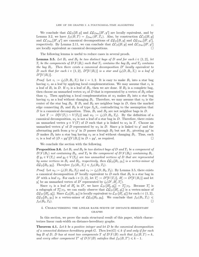
Theorem 4.1. Let k be a positive integer and let D be the canonical decompositionof a connected distance-hereditary graph G. Then lrwpGq ď k if and only if for eachbag B of D, D has at most two components T of DzV pBq such that fDpB, T q “ k,and every other component T 1 of DzV pBq satisfies that fDpB, T 1q ď k ´ 1.

12 I. ADLER, M.M. KANTE, AND O. KWON
Let D be the canonical decomposition of a connected distance-hereditary graphG, and we fix a positive integer k. For simpler arguments, we remove D from thenotation fDpB, T q in this section. We first prove the forward direction.
Proof of the forward direction of Theorem 4.1. Suppose that there exists a bag B
of D such that DzV pBq has at least three components T which induce limbs L
where GrLs has linear rank-width k.We claim that lrwpGq ě k ` 1. We may assume that DzV pBq has exactly three
components T1, T2 and T3, where each component Ti satisfies fpB, Tiq “ k. For each1 ď i ď 3, let wi :“ ζtpD,B, Tiq, and let Ni be the set of the unmarked vertices ofTi that are linked to wi in Ti. Choose a vertex ui in Ni and let Di :“ LDrB, uis. Weremark that Ni is exactly the set of the vertices in V pGrDisq that have a neighborin V pGrDsqzV pGrDisq. Since removing a vertex from a graph does not increasethe linear rank-width, we may assume that V pBq “ tζbpD,B, Tiq | 1 ď i ď 3u.Now, every unmarked vertex of D is contained in one of T1, T2, and T3. Moreover,by Proposition 3.3 and Lemmas 2.3 and 2.11, for any canonical decomposition D1
locally equivalent to D, we have lrwpGrDsq “ lrwpGrD1sq and fpB, Tiq does notchange. So, we may assume that B is a complete bag of D.
We first claim that D2 “ pD ˚ u1qrV pT2qzw2s. Since B is a complete bag, by thedefinition of limbs, D2 “ T2 ˚ w2zw2. Since u1 is linked to w1 in T1 and there is analternating path from w1 to w2 in D, by concatenating alternating paths it is easyto see that pD ˚ u1qrV pT2qzw2s “ T2 ˚ w2zw2 “ D2, as claimed.
Towards a contradiction, suppose that GrDs has a linear layout L of width k.Let a and b be the first vertex and the last vertex of L, respectively. Since B
has no unmarked vertices, without loss of generality, we may assume that a, b PV pGrD1sq YV pGrD3sq. With this assumption, we claim that GrD2s has linear rank-width at most k ´ 1.
Let v P V pGrD2sq and Sv :“ tx P V pGrDsq | x ďL vu and Tv :“ V pGrDsqzSv.Since v is arbitrary, it is sufficient to show that cutrkGrD2spSv XV pGrD2sqq ď k ´ 1.
We divide into three cases. We first check two cases that are (1) (N1 X Sv ‰ Hand N3 X Tv ‰ H), and (2) (N1 X Tv ‰ H and N3 X Sv ‰ H). If both of them arenot satisfied, then we can easily deduce that N1 Y N3 Ď Sv or N1 Y N3 Ď Tv.
Case 1. N1 X Sv ‰ H and N3 X Tv ‰ H.Let x1 P N1 X Sv and x3 P N3 X Tv. We claim that
cutrkGrD2spSvXV pGrD2sqq “ cutrkpGrDsqrV pGrD2sqYtx1,x3usppSvXV pGrD2sqqYtx1uq´1.
Because cutrkpGrDsqrV pGrD2sqYtx1,x3usppSv XV pGrD2sqq Y tx1uq ď cutrkGrDspSvq ď k,
the claim implies that cutrkGrD2spSv X V pGrD2sqq ď k ´ 1.Note that x1 and x3 have the same neighbors in pGrDsqrV pGrD2sq Y tx1, x3us
because B is a complete bag. Since x1 is adjacent to x3 in pGrDsqrV pGrD2sq Ytx1, x3us, x3 becomes a leaf in pGrDsqrV pGrD2sq Y tx1, x3us ˚ x1 whose neighbor isx1. Since pD ˚ x1qrV pT2qzw2s “ D2, we have
pGrDsqrV pGrD2sq Y tx1, x3us ˚ x1zx1zx3 “ pGrDs ˚ x1qrV pGrD2sqs “ GrD2s.

LRW OF DH GRAPHS I: A POLYNOMIAL-TIME ALGORITHM 13
Therefore,
cutrkpGrDsqrV pGrD2sqYtx1,x3usppSv X V pGrD2sqq Y tx1uq
“ cutrkpGrDsqrV pGrD2sqYtx1,x3us˚x1ppSv X V pGrD2sqq Y tx1uq
“ rank
¨˚˝
x3 Tv X V pGrD2sqˆ ˙x1 1 ˚
Sv X V pGrD2sq 0 ˚
˛‹‹‚
“ rank
¨˚˝
x3 Tv X V pGrD2sqˆ ˙x1 1 0
Sv X V pGrD2sq 0 ˚
˛‹‹‚
“ cutrkpGrDsqrV pGrD2sqYtx1,x3us˚x1zx1zx3pSv X V pGrD2sqq ` 1
“ cutrkpGrD2sqpSv X V pGrD2sqq ` 1,
as claimed.
Case 2. N1 X Tv ‰ H and N3 X Sv ‰ H.In the same way as Case 1, we can prove cutrkGrD2spSv X V pGrD2sqq ď k ´ 1.
Case 3. N1 Y N3 Ď Sv or N1 Y N3 Ď Tv.We can assume without loss of generality that N1 Y N3 Ď Sv because the case
when N1 Y N3 Ď Tv is similar. Since a, b P V pGrD1sq Y V pGrD3sq and the graphpGrDsqrV pGrD1sqYV pGrD3sqs is connected, there exist vertices s P SvXpV pGrD1sqYV pGrD3sqq and t P Tv X pV pGrD1sq Y V pGrD3sqq such that
(1) st P EpGrDsq,(2) t has no neighbors in N2.
We have
cutrkGrDspSvq ě rank
¨˚˝
t Tv X V pGrD2sqˆ ˙s 1 ˚
Sv X V pGrD2sq 0 ˚
˛‹‹‚
“ rank
¨˚˝
t Tv X V pGrD2sqˆ ˙s 1 0
Sv X V pGrD2sq 0 ˚
˛‹‹‚
“ cutrkGrD2spSv X V pGrD2sqq ` 1.
Therefore, we conclude cutrkGrD2spSv X V pGrD2sqq ď k ´ 1.Thus, GrD2s has linear rank-width at most k´1, which yields a contradiction. �
To prove the converse direction, we use the following lemmas. For two linearlayouts px1, . . . , xnq, py1, . . . , ymq, we define
px1, . . . , xnq ‘ py1, . . . , ymq :“ px1, . . . , xn, y1, . . . , ymq.
Lemma 4.2. Let B be a bag of D of type S with two unmarked vertices x and y
such that x is the center and y is a leaf of B. If for every component T of DzV pBq,fpB, T q ď k ´ 1, then the graph GrDs has a linear layout of width at most k whosefirst and last vertices are x and y, respectively.
Proof. Let T1, T2, . . . , Tℓ be the components of DzV pBq and for each 1 ď i ď ℓ, letwi :“ ζtpD,B, Tiq and let yi be a vertex in Ti represented by a vertex of B. Sinceeach wi is adjacent to a leaf of B, Tizwi is the limb of D with respect to B and yi.Let A :“ V pBqzp
Ť1ďjďℓtζbpD,B, Tiquqztx, yu, and let LA be a sequence of A.

14 I. ADLER, M.M. KANTE, AND O. KWON
Suppose that for every component T of DzV pBq, fpB, T q ď k ´ 1. For each1 ď i ď ℓ, let Li be a linear layout of GrTizwis of width at most k ´ 1. We claimthat
L :“ pxq ‘ L1 ‘ L2 ‘ ¨ ¨ ¨ ‘ Lℓ ‘ LA ‘ pyq
is a linear layout of GrDs of width at most k. It is sufficient to prove that for everyw P V pGrDsqztx, yu, cutrkGrDsptv | v ďL wuq ď k.
Letw P V pGrDsqzpAYtx, yuq, and let Sw :“ tv : v ďL wu and Tw :“ V pGrDsqzSw.Let j be the integer such that Lj contains w. Then
cutrkGrDspSwq
“ rank
¨˚˚
y A Tw X V pGrTjsq TwztyuzAzV pGrTjsq˜ ¸x 1 1 ˚ ˚
Sw X V pGrTjsq 0 0 ˚ 0SwztxuzV pGrTjsq 0 0 0 0
˛‹‹‹‚
“ rank
¨˚˚
y A Tw X V pGrTjsq TwztyuzAzV pGrTjsq˜ ¸x 1 0 0 0
Sw X V pGrTjsq 0 0 ˚ 0SwztxuzV pGrTjsq 0 0 0 0
˛‹‹‹‚
“ cutrkGrTjzwjspSw X V pGrTjsqq ` 1 ď pk ´ 1q ` 1 “ k.
If w P A, then it is easy to show that cutrkGrDsptv | v ďL wuq ď 1. Therefore,L is a linear layout of GrDs of width k whose first and last vertices are x and y,respectively. �
Lemma 4.3. Let B be a bag of D with two unmarked vertices x and y. If for everycomponent T of DzV pBq, fpB, T q ď k ´ 1, then the graph GrDs has a linear layoutof width at most k whose first and last vertices are x and y, respectively.
Proof. Suppose that fpB, T q ď k´1 for every component T of DzV pBq. We obtaina decomposition D1 from D as follows:
‚ If B is a complete graph, then let D1 :“ D ˚ x.‚ If B is a star whose center is x, then let D1 :“ D.‚ If y is the center of B, then let D1 :“ D ^ xy.‚ Otherwise let D1 :“ D ^ xz where z is an unmarked vertex represented by
the center of B.
It is clear that D1rV pBqs is a star whose center is x. By Proposition 3.3, foreach component T of DzV pBq, fpB, T q “ fD1 pD1rV pBqs, D1rV pT qsq. Thus, byLemma 4.2, GrD1s has a linear layout of width at most k whose first and lastvertices are x and y, respectively. Since GrD1s is locally equivalent to GrDs, weconclude that GrDs also has such a linear layout. �
Lemma 4.4. If
(1) for each bag B of D, there are at most two components T of DzV pBq sat-isfying fpB, T q “ k, and
(2) for every other component T 1 of DzV pBq, fpB, T 1q ď k ´ 1, and(3) P is the set of nodes v in TD such that exactly two components T of
DzV pbvpDqq satisfy fpbvpDq, T q “ k,
then either P “ H or TDrP s is a path.
Proof. Suppose that P ‰ H. If P has two distinct vertices v1 and v2, thenthere exists a component T1 of DzV pbDpv1qq not containing V pbDpv2qq such thatfpbDpv1q, T1q “ k, and there exists a component T2 of DzV pbDpv2qq not containing

LRW OF DH GRAPHS I: A POLYNOMIAL-TIME ALGORITHM 15
V pbDpv1qq such that fpbDpv2q, T2q “ k. By Proposition 3.6, for every node v onthe path from v1 to v2 in TD, v must be contained in P . So P induces a tree in TD.
Suppose now that P contains a node v having three neighbor bags v1, v2, and v3 inP . Then, again by Proposition 3.6, D must have three components T ofDzV pbDpvqqsuch that fpbDpvq, T q “ k, which contradicts the assumption. Therefore, P inducesa path in TD. �
Lemma 4.5. If
(1) for each bag B of D, there are at most two components T of DzV pBq sat-isfying fpB, T q “ k, and
(2) fpB, T 1q ď k ´ 1 for all the other components T 1 of DzV pBq,
then TD has a path P such that for each node v in P and each component T ofDzV pbvpDqq not containing a bag bwpDq with w P V pP q, fpB, T q ď k ´ 1.
Proof. Let P 1 be the set of nodes v in TD such that exactly two components T ofDzV pbDpvqq satisfy fpbDpvq, T q “ k. By Lemma 4.4, either P 1 “ H or TDrP 1s is apath.
We first assume that P 1 ‰ H. Let TDrP 1s “ v1v2 ¨ ¨ ¨ vn, and for each 1 ď i ď n,let Bi :“ bDpviq. By the definition, there exists a component T1 of DzV pB1q suchthat T1 does not contain a bag bDpwq with w P V pP 1q and fpB1, T1q “ k. Let v0be the node of TD such that bDpv0q is the bag of T1 that is the neighbor bag of B1
in D. Similarly, there exists a component Tn of DzV pBnq such that Tn does notcontain a bag bDpwq with w P V pP 1q and fpBn, Tnq “ k. Let vn`1 be the node ofTD such that bDpvn`1q is the bag of Tn that is the neighbor bag of Bn in D. ThenP :“ v0v1v2 ¨ ¨ ¨ vnvn`1 is the required path.
Now we assume that P 1 “ H. We choose a node v0 in TD and let B0 :“ bDpv0q.If D has no component T of DzV pB0q such that fpB0, T q “ k, then P :“ v0 satisfiesthe condition. If not, we take a maximal path P :“ v0v1 ¨ ¨ ¨ vn`1 in TD such that(with Bi :“ bDpviq)
– for each 0 ď i ď n, DzV pBiq has one component Ti such that fpBi, Tiq “ k,and Bi`1 is the bag of Ti that is the neighbor bag of Bi in D.
By the maximality of P , P is a path in TD such that for each node v of P
and a component T of DzV pbDpvqq not containing a bag bDpwq with w P V pP q,fpbDpvq, T q ď k ´ 1. �
We are now ready to prove the converse direction of the proof of Theorem 4.1.
Proof of the backward direction of Theorem 4.1. Suppose that for each bag B of D,at most two components T of DzV pBq induce limbs L where GrLs has linear rank-width exactly k, and all other component T 1 of DzV pBq induce limbs L1 whereGrL1s has linear rank-width at most k ´ 1. We claim that lrwpGq ď k.
Let P :“ v0v1 ¨ ¨ ¨ vnvn`1 be the path in TD such that
‚ for each node v in P and a component T of DzV pbDpvqq not containing abag bDpwq with w P P , fpbDpvq, T q ď k ´ 1 (such a path exists by Lemma4.5).
For each 0 ď i ď n ` 1, let Bi :“ bDpviq. If P consists of one vertex, then byLemma 4.3, lrwpGq “ lrwpGrDsq ď k. Thus, we may assume that n ě 0.
By adding unmarked vertices in B0 and Bn`1 if necessary, we assume that B0
and Bn`1 have unmarked vertices a0 and bn`1 in D, respectively.For each 0 ď i ď n, let bi be a marked vertex of Bi and let ai`1 be a marked
vertex Bi`1 such that biai`1 is the marked edge connecting Bi and Bi`1. Let D0
be the component of DzV pB1q containing the bag B0. Let Dn`1 be the componentof DzV pBnq containing the bag Bn`1. For each 1 ď i ď n, let Di be the componentof DzpV pBi´1q Y V pBi`1qq containing the bag Bi. Notice that the vertices ai andbi are unmarked vertices in Di.

16 I. ADLER, M.M. KANTE, AND O. KWON
Since every component T of DizV pBiq satisfies that fDipBi, T q ď k ´ 1, by
Lemma 4.3, GrDis has a linear layout L1i of width k whose first and last vertices are ai
and bi, respectively. For each 1 ď i ď n, let Li be the linear layout obtained from L1i
by removing ai and bi. Let L0 and Ln`1 be obtained from L10 and L1
n`1 by removingb0 and an`1, respectively. Then we can easily check that L :“ L0 ‘L1 ‘ ¨ ¨ ¨ ‘Ln`1
is a linear layout of GrDs having width at most k. Therefore lrwpGrDsq ď k. �
5. Canonical limbs
We investigate useful properties of canonical limbs which will be used to designour algorithm. Note that for recursively taking limbs, we need to transform anobtained limb into a canonical limb because limbs are only defined on canonicaldecompositions. Let D be the canonical decomposition of a connected distance-hereditary graph.
Proposition 5.1. Let B1 and B2 be two distinct bags of D and for each i P t1, 2u,let Ti be the component of DzV pBiq, wi :“ ζbpD,Bi, Tiq and yi be an unmarkedvertex of D represented by wi such that
‚ T1 contains the bag B2 and T2 contains the bag B1, and‚ V pB1q induces a bag in LCDrB2, y2s, and V pB2q induces a bag in LCDrB1, y1s.
We define that
‚ B11 :“ pLCDrB2, y2sqrV pB1qs,
‚ B12 :“ pLCDrB1, y1sqrV pB2qs,
‚ y11 is an unmarked vertex of LCDrB2, y2s represented by w1, and
‚ y12 is an unmarked vertex of LCDrB1, y1s represented by w2.
Then LCLCDrB1,y1srB12, y
12s is locally equivalent to LCLCDrB2,y2srB
11, y
11s.
Proof. For each i P t1, 2u, let vi :“ ζtpD,Bi, Tiq. By Lemma 3.5, there exists acanonical decompositionD1 locally equivalent toD such that for each i P t1, 2u, wi isa leaf of D1rV pBiqs in D1. For each i P t1, 2u, let Pi :“ D1rV pBiqs, T 1
i :“ D1rV pTiqs,and zi be an unmarked vertex of D1 represented by wi. We define that
‚ T 1 :“ D1rV pT 11q X V pT 1
2qs,‚ P 1
1 :“ pLCD1 rP2, z2sqrV pP1qs,‚ P 1
2 :“ pLCD1 rP1, z1sqrV pP2qs,‚ let z1
1 be an unmarked vertex of LCD1 rP2, z2s represented by w1,‚ let z1
2 be an unmarked vertex of LCD1 rP1, z1s represented by w2.
Since D is locally equivalent to D1, by Proposition 3.3, LCDrB1, y1s is locallyequivalent to LCD1 rP1, z1s. Again, since LCDrB1, y1s is locally equivalent to LCD1 rP1, z1s,by Proposition 3.3,
LCLCDrB1,y1srB12, y
12s is locally equivalent to LCLCD1 rP1,z1srP
12, z
12s.
Similarly, we obtain that
LCLCDrB2,y2srB11, y
11s is locally equivalent to LCLCD1 rP2,z2srP
11, z
11s.
Since each vi is a leaf of Pi in D1,
LLD1 rP1,z1srP12, z
12s “ T 1zv1zv2 “ LLD1 rP2,z2srP
11, z
11s,
and it implies that
LCLCD1 rP1,z1srP12, z
12s “ LCLCD1 rP2,z2srP
11, z
11s.
Therefore, LCLCDrB1,y1srB12, y
12s is locally equivalent to LCLCDrB2,y2srB
11, y
11s. �
Proposition 5.2. Let B1 and B2 be two distinct bags of D. Let T1 be a componentof DzV pB1q that does not contain B2 and T2 be the component of DzV pB2q con-taining the bag B1. For i P t1, 2u, let wi :“ ζbpD,Bi, Tiq, and yi be an unmarkedvertex of D represented by wi. If V pB1q induces a bag B1
1 of LCDrB2, y2s, then

LRW OF DH GRAPHS I: A POLYNOMIAL-TIME ALGORITHM 17
LCDrB1, y1s is locally equivalent to LCLCDrB2,y2srB11, y
11s, where y1
1 is an unmarkedvertex of LCDrB2, y2s represented by w1.
Proof. Suppose V pB1q induces a bag B11 of LCDrB2, y2s and y1
1 is an unmarkedvertex represented in LCDrB2, y2s by w1. By Lemma 3.5, there exists a canoni-cal decomposition D1 locally equivalent to D such that w2 is a leaf of a star bagD1rV pB2qs. We define
‚ P1 :“ D1rV pB1qs,‚ P2 :“ D1rV pB2qs,‚ for each i P t1, 2u, zi is an unmarked vertex of D1 represented by wi,‚ P 1
1 :“ pLCD1 rP2, z2sqrV pB1qs, and‚ z1
1 is an unmarked vertex of LCD1 rP2, z2s represented by w1.
Since D is locally equivalent to D1, by Proposition 3.3, LCDrB1, y1s is locallyequivalent to LCD1 rP1, z1s. Similarly, we obtain that LCDrB2, y2s is locally equiv-alent to LCD1 rP2, z2s. Since LCDrB2, y2s is locally equivalent to LCD1 rP2, z2s, byProposition 3.3,
LCLCDrB2,y2srB11, y
11s is locally equivalent to LCLCD1 rP2,z2srP
11, z
11s.
Since w2 is a leaf of P2 in D1, LCD1 rP1, z1s “ LCLCD1 rP2,z2srP11, z
11s, and therefore,
LCDrB1, y1s is locally equivalent to LCLCDrB2,y2srB11, y
11s, as required. �
6. Computing the linear rank-width of distance-hereditary graphs
We describe an algorithm to compute the linear rank-width of distance-hereditarygraphs. Since the linear rank-width of a graph is the maximum linear rank-widthover all its connected components, we will focus on connected distance-hereditarygraphs.
Theorem 6.1. The linear rank-width of every connected distance-hereditary graphwith n vertices can be computed in time Opn2 ¨ log2 nq. Moreover, a linear layoutof the graph witnessing the linear rank-width can be computed with the same timecomplexity.
The main idea consists of rooting the canonical decomposition D of a connecteddistance-hereditary graph and associating each bag B of D with a canonical limbLCDrB1, ys where B1 is the parent of B and y is an unmarked vertex in somedescendant bag of B, and computing the linear rank-width of LGDrB1, ys. FollowingTheorem 4.1, in order to compute the linear rank-width of LGDrB1, ys, we need tocheck the linear rank-width of proper limbs obtained from LCDrB1, ys by removingsome bags of LCDrB1, ys. Basically, we need to take canonical limbs recursivelyfrom this reason. In contrast to the case of forests for computing path-width,the associated canonical limbs here are not necessarily sub-decompositions of theoriginal decomposition, and thus, it is not at all trivial how to store values to usein the next steps. The crucial point of achieving our running time is to overcomethis problem using the results in Section 5.
Rooted decomposition trees. We define the notion of rooted decomposition trees.A decomposition tree is rooted if we distinguish either a node or an edge and callit the root of the tree. Let T be a rooted decomposition tree with the root r. Anode v is a descendant of a node v1 if v1 is in the unique path from the root to v,and when r is a marked edge, this path contains both end vertices of r. If v is adescendant of v1 and v and v1 are adjacent, then we call v a child of v1 and v1 theparent of v. Observe from the definition of descendants that if r “ vv1, then v is theparent of v1 and also v1 is the parent of v. We allow this tricky part for a technicalreason. A node in T is called a non-root node if it is not the root node.
Two nodes v and v1 are called comparable if one node is a descendant of theother one. Otherwise, they are called incomparable. Recall that for each node v of

18 I. ADLER, M.M. KANTE, AND O. KWON
T and each canonical decomposition D with T as its decomposition tree we writebDpvq to denote the bag of D with which it is in correspondence. For convenience,let pbDpvq :“ bDpv1q with v1 the parent of v.
Let D be the canonical decomposition of a connected distance-hereditary graphG and let T be its decomposition tree rooted at r. Let B :“ bDpvq for some non-rootnode v of T , and let y be an unmarked vertex of D that is represented by a vertex
of B. We define the root of the decomposition tree rT of LCDrB, ys as follows. We
assume that rT is obtained from T by removing v, and possibly adding an edge oridentifying two nodes following the definition of canonical limbs. If two comparablenodes w and w1 with w the parent of w1 are identified, then let w be the identifiednode. Otherwise, we give a new label for the identified node.
(1) If r exists in rT , then we assign r as the root of rT . In the other cases, wecan observe that either
‚ r is the root node and bDprq is removed when taking the canonicallimb or
‚ r is the root edge, and a bag bDpr1q is removed where r1 is a nodeincident with the root edge, when taking the canonical limb.
(2) If the removed node has one neighbor in T zr, then we assign this neighbor
as the root of rT .(3) If the removed node has two neighbors in T zr and they are linked by a new
edge in rT , then we assign the new edge as the root of rT .(4) If the removed node has two neighbors in T zr and they are identified in rT ,
then we assign the new node as the root of rT .The following observation is easy to check from the definition of rooted decom-
position trees of canonical limbs.
Fact 6.2. If w is a non-root node of the rooted decomposition tree rT of a canon-ical limb LCDrB, ys, then w is also a non-root node of T with the property thatV pbDpwqq “ V pbLCDrB,yspwqq.
k-critical nodes. For every non-root node v of T with the parent node v1, wedefine that
‚ T1rD, vs is the component of DzV pbDpv1qq containing bDpvq,‚ T2rD, vs is the component of DzV pbDpvqq containing bDpv1q,‚ f1pD, vq :“ fDppbDpvq, T1rD, vsq,‚ f2pD, vq :“ fDpbDpvq, T2rD, vsq,‚ ζ1pD, vq :“ ζbpD, bDpv1q, T1rD, vsq, and‚ ζ2pD, vq :“ ζbpD, bDpvq, T2rD, vsq.
A node v of T is called k-critical if f1pD, vq “ k and v has two children v1 and v2such that f1pD, v1q “ f1pD, v2q “ k.
From now on, we define some sequences of canonical limbs, which will be takensequentially in our algorithm. We recall that lrwpGq ď log2|V pGq| by Theorem 2.1and Lemma 2.2. For convenience, let
η :“ tlog2|V pGq|u.
For each non-root node v of T , we define recursively the following. We first choosean unmarked vertex y of D represented by ζ1pD, vq, and
‚ let Dvη be any canonical limb LCDrpbDpvq, ys, and let T v
η be the rooteddecomposition tree of Dv
η.
For each 1 ď j ď η, let αvj :“ maxtf1pDv
j , wq | w is a non-root node of T vj u, and we
define Dvj´1 and T v
j´1 as follows:
(1) If αvj ‰ j, then let Dv
j´1 :“ Dvj and T v
j´1 :“ T vj .

LRW OF DH GRAPHS I: A POLYNOMIAL-TIME ALGORITHM 19
(2) If αvj “ j and one of the following is satisfied, then let Dv
j´1 :“ Dvj and
T vj´1 :“ T v
j .
‚ T vj has a node with at least 3 children w such that f1pDv
j , wq “ j.‚ T v
j has two incomparable nodes v1 and v2 where v1 is a j-critical node
v1 and f1pDvj , v2q “ j.
‚ T vj has no j-critical nodes.
(3) Otherwise, T vj has the unique j-critical node vc. In this case, we choose
an unmarked vertex y of Dvj represented by ζ2pDv
j , vcq and let Dvj´1 :“
LCDvjrbDv
jpvcq, ys and let T v
j´1 be the rooted decomposition tree of Dvj´1.
Lastly for each 0 ď j ď η, let βvj :“ lrwpGrDv
j sq.The existence of the unique j-critical node in (3) is verified in the next proposi-
tion.
Proposition 6.3. Let 0 ď j ď η and let v be a non-root node of T such that αvj ď j
and T vj contains neither
‚ a node having at least 3 children w with f1pDvj , wq “ αv
j , nor‚ two incomparable nodes v1 and v2 having the property that v1 is an αv
j -critical node and f1pDv
j , v2q “ αvj .
Let w be an αvj -critical node of T v
j . Then w is the unique αvj -critical vertex of T v
j .Moreover, lrwpGrDv
j sq “ αvj ` 1 if and only if lrwpGrDv
j´1sq “ f2pDvj , wq “ αv
j .
Proof. Let k :“ αvj . We first show that w is the unique k-critical node of T v
j . Let w1
be a k-critical node of T vj that is distinct from w. From the second assumption, w
and w1 must be comparable in T vj . Without loss of generality, we may assume that
w is a descendant of w1 in T vj . Then by the definition of k-criticality, w1 has a child
w2 such that f1pDvj , w
2q “ k and w is not a descendant of w2 in T vj , contradicting
to the second assumption.Now we claim that lrwpGrDv
j sq “ k ` 1 if and only if f2pDvj , wq “ k. By the
assumption on k and by Theorem 4.1, lrwpGrDvj sq ď k ` 1. Let w1 and w2 be the
two children of w such that f1pDvj , w1q “ f1pDv
j , w2q “ k. By assumption, every
other child w1 of w satisfies that f1pDvj , w
1q ď k ´ 1.
If f2pDvj , wq “ k, then clearly we have lrwpGrDv
j sq ě k ` 1 by Theorem 4.1.For the forward direction, suppose that lrwpGrDv
j sq ě k ` 1. Since T vj contains no
node having at least three children w such that f1pDvj , wq “ k, by Theorem 4.1,
there should exist a k-critical node vc of T vj such that f2pDv
j , vcq “ k. Since w is
the unique k-critical node of T vj , w “ vc and f2pDv
j , wq “ lrwpGrDvj´1sq “ k, as
required. �
Let v be a non-root node of T . From Theorem 4.1, we can easily observe thatαvη ď lrwpGrDv
ηqsq ď αvη ` 1. By Proposition 6.3, if T v
η has no unique critical node,then it is easy to determine βv
η , and otherwise the computation of βvη can be reduced
to the computation of f2pDvη, vcq where vc is the unique αv
η-critical node of T vη . In
order to compute it, we can recursively call the algorithm on GrDvαv
η´1s. However,
we will prove that these recursive calls are not needed if we store the values βvj .
Lemma 6.4. Let v be a non-root node of T . Let i be an integer such that 0 ď i ă η.If αv
i ď i, then αvi`1 ď i ` 1.
Proof. Suppose that αvi`1 ě i`2. By the definition ofDv
i , Dvi “ Dv
i`1 and therefore,αvi ě i ` 2, which yields a contradiction. �
Our algorithm. Now we are ready to present and analyze our algorithm. Wedescribe the algorithm explicitly in Algorithm 2. First, we modify the given decom-position as follows. For the canonical decomposition D1 of a distance-hereditary

20 I. ADLER, M.M. KANTE, AND O. KWON
graph G, we modify D1 into a canonical decomposition D of a connected distance-hereditary graph by adding a root bag R and making it adjacent to a bag R1 ofD1 so that f1pD, vq “ lrwpGq, where v is the node corresponding to the bag R1.We call pD,Rq a modified canonical decomposition of G. Let T be the decomposi-tion tree of the new canonical decomposition D. The basic strategy is to computeβvi “ lrwpGrDv
i sq for all non-root nodes v of T and all integers i such that αvi ď i.
We recall that η “ tlog2|V pGq|u.We first present the subroutine Limb which computes a canonical limb and its
decomposition tree recursively.
Algorithm 1: Limb(D,T, tγpvq | v P V pT zrqu, w P V pT zrq, z P t1, 2u).
Input: A canonical decomposition D of a connected distance-hereditary graph, its
rooted decomposition tree T with the root r, tγpvq P N | v P V pT zrqu, anon-root node w of T , and z P t1, 2u.
Output: A canonical decomposition D1 of D associated with TzrD,ws, its rooted
decomposition tree T 1 with the root r1, tγpvq | v P V pT 1zr1qu, and α.
1 Let w1 be the parent of w;
2 if z “ 1 then choose an unmarked vertex y of D represented by ζ1pD,wq and
v Ð w1; else choose an unmarked vertex y of D represented by ζ2pD,wq and v Ð w;
D1 Ð LCDrbDpvq, ys and obtain T 1 from T and assign the root r1 of T 1;
3 α Ð maxtγpvq | v P V pT 1zr1qu;
4 return pD1, T 1, tγpvq | v P V pT 1zr1qu, αq;
We describe the main algorithm in Algorithm 2.
Correctness of the algorithm. The following proposition has a key role in thealgorithm. It mainly uses the results in Section 5.
Proposition 6.5. Let v be a non-root node of T and let 0 ď i ď η such that αvi ď i.
If w is a non-root node of T vi , then, β
wi “ f1rDv
i , ws.
Proof. Let w be a non-root node of T vi . By Fact 6.2, for each i ` 1 ď j ď η,
w P V pT vj q and hence w P V pT q. Moreover, since αv
i ď i, by Lemma 6.4, αvj ď j for
all i ` 1 ď j ď η. For each i ď j ď η, we define that
‚ yj is an unmarked vertex of Dvj represented by the marked vertex ζ1pDv
j , wq.
Now, we claim that for each i ď j ď η,
‚ LCDvjrpbDv
jpwq, yjs is locally equivalent to Dw
j .
If it is true, then we obtain that LCDvirpbDv
ipwq, yis is locally equivalent to Dw
i ,
which implies that βwi “ f1rDv
i , ws. We prove it by induction on η ´ j.If j “ η, then both Dv
η and Dwη are canonical limbs of D. Since w is a non-root
node of T vη , V pbDpwqq induces a bag in Dv
η , and hence by Proposition 5.2, Dwη is
locally equivalent to LCDvηrpbDv
ηpwq, yηs.
Now let us assume that i ď j ă η. By induction hypothesis Dwj`1 is locally
equivalent to LCDvj`1
rpbDvj`1
pwq, yj`1s. Assume first that αvj`1 ď j. Then, by
Proposition 5.2, we have that αwj`1 ď j. In that case, by the definition, we have
Dvj “ Dv
j`1 and Dwj “ Dw
j`1, and we conclude the statement.Assume now that αv
j`1 “ j`1. Since αvj`1 “ j`1 and αv
j ď j, T vj`1 should have
a unique pj ` 1q-critical node vc such that Dvj “ LCDv
j`1rbDv
j`1pvcq, ycs for some
unmarked vertex yc of Dvj`1 represented by ζ2pDv
j`1, vcq. We distinguish two cases:either vc is incomparable with w in T v
j`1, or vc is a descendant of w in T vj`1. Since
w is a node of T vj , w cannot be a descendant of vc.
Case 1. vc is incomparable with w in T vj`1.

LRW OF DH GRAPHS I: A POLYNOMIAL-TIME ALGORITHM 21
Algorithm 2: Compute Linear Rank-Width of Connected Distance-
Hereditary GraphsInput: A connected distance-hereditary graph G.
Output: The linear rank-width of G.
1 Compute a modified canonical decomposition pD,Rq of G, and the decomposition
tree T of D with the root node r;
2 Let βvi Ð 0 for each non-root node and each 0 ď i ď η;
3 For each non-root leaf node v in T and each 0 ď i ď η, let βvi Ð 1 ;
4 Γ Ð tβvi | v P V pT zrqu;
5 while T has a non-root node v where βvη is not computed do
6 Let v be a non-root node in T where βvη “ 0, but βv1
η ‰ 0 for each child v1 of v;
7 pDvη , T
vη ,Γ
vη, α
vηq Ð Limb(D,T,Γ, v, 1);
8 Let S be a stack; i Ð αvη; k Ð αv
η;
9 while (true) do
10 if (T vi has a node having at least 3 children v1 with βv1
i “ i) or (T vi has two
incomparable nodes v1 and v2 having the property that v1 is an i-critical nodeand β
v2i “ i) or (T v
i has no i-critical nodes) then11 Stop this loop
12 Find the unique i-critical node vc of T vi ;
13 pDvi´1, T
vi´1,Γ
vi´1, α
vi´1q Ð Limb(Dv
i , Tvi ,Γ
vi , vc, 2);
14 pushpS, iq and i Ð αvi´1;
15 if (T vi has a node having at least 3 children v1 with βv1
i “ i) or (T vi has two
incomparable nodes v1 and v2 with the property that v1 is an i-critical node andβv2i “ i) then βv
i Ð i ` 1; else βvi Ð i; while pS ‰ Hq do
16 j Ð pullpSq;
17 if βvi “ j then βv
j Ð j ` 1; else βvj Ð j; for ℓ Ð i ` 1 to j ´ 1 do
18 βvℓ Ð βv
i ;
19 i Ð j;
20 for j Ð k ` 1 to η do21 βv
j Ð βvk ;
22 Let r1 be the unique neighbor of the root and return βr1
η ;
Since vc is incomparable with w in T vj`1 and vc is the unique pj `1q-critical node
in T vj`1, there is no pj ` 1q-critical node in Tw
j`1. Hence, Dwj “ Dw
j`1 by definition.Also, by Proposition 5.2,
‚ LCDvjrpbDv
jpwq, yjs is locally equivalent to LCDv
j`1rpbDv
j`1
pwq, yj`1s.
Hence, we can conclude that Dwj is locally equivalent to LCDv
jrpbDv
jpwq, yj s because
Dwj`1 is locally equivalent to LCDv
j`1rpbDv
j`1
pwq, yj`1s.
Case 2. vc is a descendant of w in T vj`1.
If vc is a child of w in T vj`1 and the bag bDv
j`1pwq has size 3, then T v
j cannot
contain w as a node, and this contradicts the assumption that w is a node of T vj .
Therefore, we may assume that either
(1) |bDj`1pwq| ě 4, or
(2) |bDj`1pwq| “ 3 and vc is not a child of w in T v
j`1.
This implies that vc is a node of the decomposition tree of LCDvj`1
rpbDvj`1
pwq, yj`1s.
Let D1 :“ LCDvj`1
rpbDvj`1
pwq, yj`1s. By induction hypothesis, we know that Dwj`1
is locally equivalent to D1. Note that, by definition vc is also the unique criticalnode of Tw
j`1, and

22 I. ADLER, M.M. KANTE, AND O. KWON
‚ Dwj “ LCDw
j`1rbDw
j`1pvcq, zs for some unmarked vertex z ofDw
j`1 represented
by ζ2pDwj`1, vcq.
Also, by Proposition 5.1,
‚ LCDvjrpbDv
jpwq, yjs is locally equivalent to LCD1 rbD1 pvcq, z1s where z1 is an
unmarked vertex of D1 represented by ζ2pD1, vcq.
Since D1 is locally equivalent to Dwj`1, LCDv
jrpbDv
jpwq, yj s is locally equivalent to
Dwj , and this concludes the proof. �
Proof of Theorem 6.1. We first show that Algorithm 2 correctly computes the linearrank-width of G. If |V pGq| ď 1, then lrwpGq “ 0 from the definition. We mayassume that |V pGq| ě 2. Let pD,Rq be a modified canonical decomposition of Gand let T be the canonical decomposition tree of D and let r1 be the unique neighborof the root of T . As we observed, we have that lrwpGq “ lrwpGrDr1
η sq “ βr1
η , and
want to prove that Algorithm 2 correctly outputs βr1
η . We claim that for each non-root node v of T and 0 ď i ď η such that αv
i ď i, Algorithm 2 correctly computesβvi .Suppose v is a non-root leaf node of T . Since every canonical limb is connected
by Lemma 3.1 and |V pGq| ě 2, Dvη is isomorphic to either a complete graph or a
star with at least two vertices. Thus, lrwpGrDvηsq “ 1, and by construction for each
0 ď i ď η, Dvi “ Dv
η, and Line 3 correctly puts these values.We assume that v is a non-root node in T that is not a leaf, and for all its
descendants v1 and integers 0 ď ℓ ď η with αv1
ℓ ď ℓ, βv1
ℓ is computed (i.e. βv1
ℓ ‰ 0).We claim that Line 9-14 recursively computes Dv
i for each i where αvi ď i. We first
remark that for computing αvi of T v
i , we use the fact that for each non-root node wof T v
i , βwi “ f1rDv
i , ws from Proposition 6.5. So, αvi “ maxtβw
i | w a non-root nodew of T v
i u.Let i P t0, 1, . . . , ηu such that αv
i ď i. If αvi ă i, then by the definition, T v
i´1 “ T vi
and thus, we take Dvi´1 “ Dv
i . We may assume that αvi “ i. If either T v
i has a node
with at least 3 children v1 such that βv1
i “ i, or T vi has two incomparable nodes v1
and v2 with v1 an i-critical node and βv2i “ i, then from the definition of Dv
i , wehave that Dv
i´1 “ Dvi and for all 0 ď ℓ ď i ´ 1, αv
ℓ “ i ą ℓ. Since we do not needto evaluate βv
ℓ when αvℓ ą ℓ, we stop the loop. If T v
i has no i-critical node, thenβvi “ αv
i “ i, that is, the βvi value cannot be increased by one. In this case, we also
stop the loop. These 3 cases are the conditions in Line 10.Suppose neither of the conditions in Line 10 occur. Then by Proposition 6.3, T v
i
has a unique i-critical bag vc and Dvi´1 is equal to a canonical limb LCDv
irbDv
ipvcq, ys
where y is some unmarked vertex of Dvi represented by ζ2pDv
i , vcq. So, we computeDv
i´1 from Dvi , the rooted decomposition tree T v
i´1 of Dvi´1 and compute subse-
quently αvi´1. Notice that for all αv
i´1 ď ℓ ď i ´ 1, Dvℓ “ Dv
i´1 and thus it issufficient in the next iteration to deal with Dv
αvi´1
directly. Thus, Line 9-14 cor-
rectly computes canonical decompositions Dvi for each i where αv
i “ i.Now we verify the procedure of computing βv
j in Line 15. Let 0 ď ℓ ď η be theminimum integer such that αv
ℓ “ ℓ. If ℓ “ 0, then βvℓ “ 1. Suppose ℓ ě 1. Then
since αvℓ´1 ą ℓ ´ 1, by Theorem 4.1, we have that
(1) βvℓ “ ℓ`1 if either T v
ℓ has a node having at least 3 children v1 with βv1
ℓ “ ℓ, ortwo incomparable nodes v1 and v2 with the property that v1 is an i-criticalnode and βv2
i “ i,(2) βv
ℓ “ ℓ if otherwise.
Thus, Line 15 correctly computes it.In the loop in Line 9, we use a stack to pile up the integers i such that T v
i hasthe unique i-critical node. When T v
i has the unique i-critical node, by Proposition6.3,

LRW OF DH GRAPHS I: A POLYNOMIAL-TIME ALGORITHM 23
(1) βvi “ i ` 1 if βv
i´1 “ i, and(2) βv
i “ i if βvi´1 ď i ´ 1.
So, from the lower value in the stack we can compute βvi recursively. From Line 15
to Line 20, Algorithm 2 computes all βvi correctly where αv
i ď i, and in particular,
it computes βvη . Therefore, at the end of the algorithm, it computes βr1
η that isequal to the linear rank-width of G.
The running time of the algorithm. Let us now analyze its running time. Letn and m be the number of vertices and edges of G. Its canonical decomposition canbe computed in time Opn ` mq by Theorem 2.7, and one can compute a modifiedcanonical decomposition pD,Rq in constant time. Note that the number of bags inD is bounded by Opnq (see [14, Lemma 2.2]).
We first remark that Algorithm 1 runs in timeOpnq. This is because when we takea limb from a canonical decomposition, we need to take a local complementation ora pivoting on a sub-decomposition, and in the worst case, we may visit each bag toapply these operations. The decomposition tree and α, β values can be obtained inlinear time.
Now we observe the running time of Algorithm 2. The number of iterations ofthe whole loop from Line 6 to Line 21 is at most Opnq because it runs in as manyas the number of bags in D. Lines 6-8 can be implemented in time Opnq. The loopin Line 9 runs log2pnq times because lrwpGq ď log2pnq, and all the steps in Line 9can be implemented in time Opnq. Also, Lines 15-20 can be done in time Opnq. Weconclude that this algorithm runs in time Opn2 ¨ log2 nq.
Finding an optimal linear layout. We finally establish how to find a linearlayout witnessing lrwpGq. We may assume that G has at least 3 vertices. We canassume that for each non-root node v of T and 0 ď i ď η with αv
i ď i, T vi and βv
i
are computed. We inductively obtain optimal linear layouts of GrDvi s using those
values. If v is a non-root leaf node of T vi , then GrDv
i s is either a complete graph ora star for all i, and thus, any ordering of V pGrDv
i sq is a linear layout of width 1.We may assume that v is a not a leaf node.
We will search for the path depicted in Lemma 4.5 to apply the same techniqueused in the proof of Theorem 4.1. What we have shown in Theorem 4.1 is that fora canonical decomposition D of a distance-hereditary graph with its decompositiontree TD, if TD has a path P :“ v0v1 ¨ ¨ ¨ vnvn`1 such that
‚ for each node v in P and a component T of DzV pbDpvqq not containing abag bDpwq with w P P , fpbDpvq, T q ď k ´ 1,
then we can generate a linear layout of GrDs having width at most k. But it assumedthat we have a linear layout of graphs corresponding to pending subtrees. So, forour purpose, it is necessary to find such a path with k “ βv
i such that
‚ for each node v in P and a component T of DzV pbDpvqq not containing abag bDpwq with w P P , a linear layout of LGDrbDpvq, T s with an optimalwidth is already computed.
Let us assume that k “ βvi . There are two cases; either T v
i has the k-criticalnode or not.
Case 1. T vi has no k-critical node.
In this case, we take a path P from the root node of T vi (or both end nodes of the
root edge) to a node w where βwi “ k but for every descendant w1 of w, βw1
i ă k.Since T v
i has no k-critical node, every node outside of this path has β value lessthan k. Thus, the graphs corresponding to subtrees pending to this path havelinear rank-width at most k´1, and moreover, by induction hypothesis, we alreadyobtained an optimal linear layout for each graph. This path can be computed inlinear time.

24 I. ADLER, M.M. KANTE, AND O. KWON
Case 2. T vi has a k-critical node.
First note that T vi cannot have two k-critical nodes, otherwise, βv
i “ k`1, whichcontradicts to our assumption. Let x be the unique k-critical node of T v
i , and letx1, x2 be two children of x where β
xj
i “ k for each j P t1, 2u. For each j P t1, 2u,we choose a descendant wj of xj where β
wj
i “ k but for every descendant w1j of wj ,
βwj
i ă k. Let P be the path from w1 to w2 in T vi . This path can be computed in
linear time.Since x is the unique k-critical node of T v
i , every node below of this path has βvalue less than k, and the graphs corresponding to subtrees pending to the path arecomputed in advance. Moreover, since this case is exactly when αv
i “ k and βvi “ k
and T vi has a unique critical node, the canonical decomposition corresponding to
the subtree of T vi zx containing the parent of x is exactly Dv
k´1, and GrDvk´1s should
have linear rank-width at most k ´ 1 as βvi “ k. By the induction hypothesis, the
optimal linear layout of GrDvk´1s is also computed before, as required.
We conclude that we can compute an optimal layout of G in time Opn2 ¨ log2 nq.�
7. Path-width of matroids with branch-width 2
As a corollary of Theorem 6.1, we can compute the path-width of matroids ofbranch-width at most 2. We first recall the necessary materials about matroids.We refer to the book written by Oxley [27] for our matroid notations.
Matroids. A pair pEpMq, IpMqq is called a matroid M if EpMq, called the groundset of M , is a finite set and IpMq, called the set of independent sets of M , is anonempty collection of subsets of EpMq satisfying the following conditions:
(I1) if I P IpMq and J Ď I, then J P IpMq,(I2) if I, J P IpMq and |I| ă |J |, then I Y tzu P IpMq for some z P JzI.
A maximal independent set in M is called a base of M . It is known that, if B1 andB2 are bases of M , then |B1| “ |B2|.
For a matroid M and a subset X of EpMq, we let pX, tI Ď X : I P IpMquq bethe matroid denoted by M X . The size of a base of M X is called the rank of Xin M and the rank function of M is the function rM : 2EpMq Ñ N that maps everyX Ď EpMq to its rank. The rank of EpMq is called the rank of M .
If M is a matroid, then we define λM , called the connectivity function of M , suchthat for every subset X of EpMq,
λM pXq “ rM pXq ` rM pEpMqzXq ´ rM pEpMqq ` 1.
It is known that the function λM is symmetric and submodular.Let A be a binary matrix and let E be the column labels of A. Let I be the
collection of all those subsets I of E such that the columns of A with index inI are linearly independent. Then MpAq :“ pE, Iq is a matroid. Every matroidisomorphic to MpAq for some matrix A is called a binary matroid and A is called arepresentation of M over the binary field.
We now define fundamental graphs of binary matroids. LetG be a bipartite graphwith a bipartition pA,Bq. We define MpG,A,Bq as the binary matroid representedby the pAˆV q-matrix pIA AGrA,Bsq where IA is the pAˆAq identity matrix; andwe call G a fundamental graph of MpG,A,Bq. We remark that |EpMq| “ |V pGq|.
Branch-width and path-width of matroids. A branch-decomposition of a ma-troid M is a pair pT, Lq, where T is a subcubic tree and L is a bijection from theelements of EpMq to the leaves of T . For an edge e in T , T ze induces a partitionpXe, Yeq of the leaves of T . The width of an edge e is defined as λM pL´1pXeqq. Thewidth of a branch-decomposition pT, Lq is the maximum width over all edges of T .

LRW OF DH GRAPHS I: A POLYNOMIAL-TIME ALGORITHM 25
The branch-width of M , denoted by bwpMq, is the minimum width over all branch-decompositions of M . If |EpMq| ď 1, then M admits no branch-decomposition andbwpMq “ 0.
A sequence e1, . . . , en of the ground set EpMq is called a linear layout of M . Thewidth of a linear layout e1, . . . , en of M is
max1ďiďn´1
tλM pte1, . . . , eiuqu.
The path-width of M , denoted by pwpMq, is defined as the minimum width over alllinear layouts of M .
The following relation is established by Oum [25].
Proposition 7.1 (Oum [25]). Let G be a bipartite graph with a bipartition pA,Bqand let M :“ MpG,A,Bq. For every X Ď V pGq, cutrkGpXq “ λM pXq ´ 1. Thus,rwpGq “ bwpMq ´ 1 and lrwpGq “ pwpMq ´ 1.
Here, we observe that every matroid of branch-width at most 2 is binary. Thiscan be observed from the known minor characterizations for binary matroids andmatroids of branch-width at most 2. For the definition of matroid minors, we referto [27].
Theorem 7.2 (Tutte [28, 29]). A matroid is binary if and only if it has no minorisomorphic to U2,4.
Theorem 7.3 (Dharmatilake [10]). A matroid has branch-width at most 2 if andonly if it has no minor isomorphic to U2,4 and MpK4q.
Corollary 7.4. The path-width of every n-element matroid of branch-width at most2 can be computed in time Opn2 ¨ log2 nq, provided that the matroid is given by anindependent set oracle. Moreover, a linear layout of the matroid witnessing thepath-width can be computed with the same time complexity.
Proof. Let M be a matroid of branch-width at most 2 and assume that an indepen-dent oracle of M is given. By Theorems 7.2 and 7.3, every matroid of branch-widthat most 2 is binary. We first run a greedy algorithm to find a base B of M [27,Section 1.8] in time Op|EpMq|q. After choosing one base B, for each e P B ande1 P EpMqzB, we test whether pBzteuq Y te1u is again a base using the independentset oracle, and we create the fundamental graph G with respect to M . It can bedone in time Op|EpMq|2q. Since M has branch-width at most 2, by Proposition 7.1,the rank-width of G is at most 1. Using Theorem 6.1, we can compute the linearrank-width of G in time Op|EpMq|2 ¨ log2|EpMq|q, which is the same as pwpMq ´1.Moreover, we can compute a linear layout witnessing lrwpGq in the same time, thatcorresponds to the linear layout of M witnessing pwpMq. �
8. An upper bound on linear rank-width
As we promised, we prove the following lemma here. We remark that Bodlaender,Gilbert, Hafsteinsson and Kloks [4] proved a similar relation between tree-width andpath-width.
Lemma 8.1. Let k be a positive integer and let G be a graph of rank-width k. ThenlrwpGq ď ktlog2|V pGq|u.
Proof. Since k is a positive integer, we have |V pGq| ě 2. Let pT, Lq be a rank-decomposition of G having width k. For convenience, we choose an edge e of T andsubdivide it with introducing a new vertex x, and regard x as the root of T . Foreach internal vertex t of T with two subtrees T1 and T2 of T zt not containing x, letℓptq :“ T1 and rptq :“ T2 if the number of leaves of T in T1 is at least the numberof leaves of T in T2. Let S be a linear layout of G satisfying that
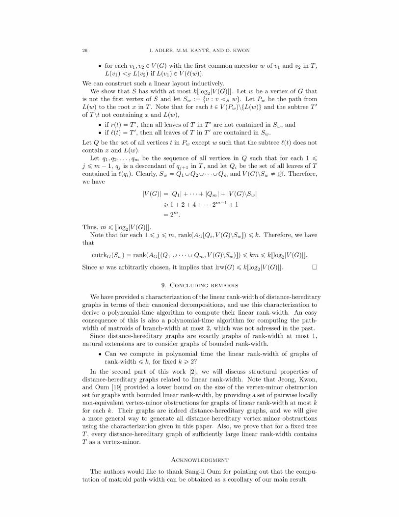
26 I. ADLER, M.M. KANTE, AND O. KWON
‚ for each v1, v2 P V pGq with the first common ancestor w of v1 and v2 in T ,Lpv1q ăS Lpv2q if Lpv1q P V pℓpwqq.
We can construct such a linear layout inductively.We show that S has width at most ktlog2|V pGq|u. Let w be a vertex of G that
is not the first vertex of S and let Sw :“ tv : v ăS wu. Let Pw be the path fromLpwq to the root x in T . Note that for each t P V pPwqztLpwqu and the subtree T 1
of T zt not containing x and Lpwq,
‚ if rptq “ T 1, then all leaves of T in T 1 are not contained in Sw, and‚ if ℓptq “ T 1, then all leaves of T in T 1 are contained in Sw.
Let Q be the set of all vertices t in Pw except w such that the subtree ℓptq does notcontain x and Lpwq.
Let q1, q2, . . . , qm be the sequence of all vertices in Q such that for each 1 ďj ď m ´ 1, qj is a descendant of qj`1 in T , and let Qi be the set of all leaves of Tcontained in ℓpqiq. Clearly, Sw “ Q1YQ2Y¨ ¨ ¨YQm and V pGqzSw ‰ H. Therefore,we have
|V pGq| “ |Q1| ` ¨ ¨ ¨ ` |Qm| ` |V pGqzSw|
ě 1 ` 2 ` 4 ` ¨ ¨ ¨ 2m´1 ` 1
“ 2m.
Thus, m ď tlog2|V pGq|u.Note that for each 1 ď j ď m, rankpAGrQi, V pGqzSwsq ď k. Therefore, we have
that
cutrkGpSwq “ rankpAGrpQ1 Y ¨ ¨ ¨ Y Qm, V pGqzSwqsq ď km ď ktlog2|V pGq|u.
Since w was arbitrarily chosen, it implies that lrwpGq ď ktlog2|V pGq|u. �
9. Concluding remarks
We have provided a characterization of the linear rank-width of distance-hereditarygraphs in terms of their canonical decompositions, and use this characterization toderive a polynomial-time algorithm to compute their linear rank-width. An easyconsequence of this is also a polynomial-time algorithm for computing the path-width of matroids of branch-width at most 2, which was not adressed in the past.
Since distance-hereditary graphs are exactly graphs of rank-width at most 1,natural extensions are to consider graphs of bounded rank-width.
‚ Can we compute in polynomial time the linear rank-width of graphs ofrank-width ď k, for fixed k ě 2?
In the second part of this work [2], we will discuss structural properties ofdistance-hereditary graphs related to linear rank-width. Note that Jeong, Kwon,and Oum [19] provided a lower bound on the size of the vertex-minor obstructionset for graphs with bounded linear rank-width, by providing a set of pairwise locallynon-equivalent vertex-minor obstructions for graphs of linear rank-width at most kfor each k. Their graphs are indeed distance-hereditary graphs, and we will givea more general way to generate all distance-hereditary vertex-minor obstructionsusing the characterization given in this paper. Also, we prove that for a fixed treeT , every distance-hereditary graph of sufficiently large linear rank-width containsT as a vertex-minor.
Acknowledgment
The authors would like to thank Sang-il Oum for pointing out that the compu-tation of matroid path-width can be obtained as a corollary of our main result.
LRW OF DH GRAPHS I: A POLYNOMIAL-TIME ALGORITHM 27
References
[1] Isolde Adler and Mamadou Moustapha Kante. Linear rank-width and linear clique-width oftrees. Theoret. Comput. Sci., 589:87–98, 2015.
[2] Isolde Adler, Mamadou Moustapha Kante, and O-joung Kwon. Linear rank-width of distance-hereditary graphs II. Vertex-minor obstructions. Submitted, 2015.http://arxiv.org/abs/1508.04718.
[3] Hans-Jurgen Bandelt and Henry Martyn Mulder. Distance-hereditary graphs. J. Comb. The-ory, Ser. B, 41(2):182–208, 1986.
[4] Hans L. Bodlaender, John R. Gilbert, Hjlmtr Hafsteinsson, and Ton Kloks. Approximatingtreewidth, pathwidth, and minimum elimination tree height. J. Algorithms, 18:238–255, 1991.
[5] Hans L. Bodlaender and Ton Kloks. Efficient and constructive algorithms for the pathwidthand treewidth of graphs. J. Algorithms, 21(2):358–402, 1996.
[6] Andre Bouchet. Transforming trees by successive local complementations. J. Graph Theory,12(2):195–207, 1988.
[7] Bruno Courcelle and Stephan Olariu. Upper bounds to the clique width of graphs. DiscreteApplied Mathematics, 101(1-3):77–114, 2000.
[8] William H. Cunnigham and Jack Edmonds. A combinatorial decomposition theory. CanadianJournal of Mathematics, 32:734–765, 1980.
[9] Elias Dahlhaus. Parallel algorithms for hierarchical clustering, and applications to split de-composition and parity graph recognition. Journal of Graph Algorithms, 36(2):205–240, 2000.
[10] Jack S. Dharmatilake. A min-max theorem using matroid separations. In Matroid theory(Seattle, WA, 1995), volume 197 of Contemp. Math., pages 333–342. Amer. Math. Soc.,Providence, RI, 1996.
[11] Reinhard Diestel. Graph theory, volume 173 of Graduate Texts in Mathematics. Springer,Heidelberg, fourth edition, 2010.
[12] Jonathan A. Ellis, Ivan Hal Sudborough, and Jonathan S. Turner. The vertex separation andsearch number of a graph. Inf. Comput., 113(1):50–79, 1994.
[13] Robert Ganian. Thread graphs, linear rank-width and their algorithmic applications. InCostas S. Iliopoulos and William F. Smyth, editors, IWOCA, volume 6460 of Lecture Notesin Computer Science, pages 38–42. Springer, 2010.
[14] Cyril Gavoille and Christophe Paul. Distance labeling scheme and split decomposition. Dis-crete Mathematics, 273(1-3):115–130, 2003.
[15] James F. Geelen, A. M. H. Gerards, and Geoff Whittle. Branch-width and well-quasi-orderingin matroids and graphs. J. Combin. Theory Ser. B, 84(2):270–290, 2002.
[16] James F. Geelen and Sang-il Oum. Circle graph obstructions under pivoting. Journal of GraphTheory, 61(1):1–11, 2009.
[17] Jim Geelen, Bert Gerards, and Geoff Whittle. Excluding a planar graph from GFpqq-representable matroids. J. Combin. Theory Ser. B, 97(6):971–998, 2007.
[18] Jim Geelen, Bert Gerards, and Geoff Whittle. Solving Rota’s conjecture. Notices Amer. Math.Soc., 61(7):736–743, 2014.
[19] Jisu Jeong, O-joung Kwon, and Sang-il Oum. Excluded vertex-minors for graphs of linearrank-width at most k. European J. Combin., 41:242–257, 2014.
[20] Mamadou Moustapha Kante. Well-quasi-ordering of matrices under Schur complement andapplications to directed graphs. European J. Combin., 33(8):1820–1841, 2012.
[21] Mamadou Moustapha Kante and Michael Rao. The rank-width of edge-coloured graphs. The-ory Comput. Syst., 52(4):599–644, 2013.
[22] Navin Kashyap. Matroid pathwidth and code trellis complexity. SIAM J. Discrete Math.,
22(1):256–272, 2008.[23] Ton Kloks, Hans L. Bodlaender, Haiko Muller, and Dieter Kratsch. Computing treewidth and
minimum fill-in: All you need are the minimal separators. In Thomas Lengauer, editor, ESA,volume 726 of Lecture Notes in Computer Science, pages 260–271. Springer, 1993.
[24] Nimrod Megiddo, S. Louis Hakimi, M. R. Garey, David S. Johnson, and Christos H. Papadim-itriou. The complexity of searching a graph. J. ACM, 35(1):18–44, 1988.
[25] Sang-il Oum. Rank-width and vertex-minors. J. Comb. Theory, Ser. B, 95(1):79–100, 2005.[26] Sang-il Oum and Paul D. Seymour. Approximating clique-width and branch-width. J. Comb.
Theory, Ser. B, 96(4):514–528, 2006.[27] James Oxley. Matroid Theory. Number 21 in Oxford Graduate Texts in Mathematics. Oxford
University Press, second edition, 2012.[28] W. T. Tutte. A homotopy theorem for matroids. I, II. Trans. Amer. Math. Soc., 88:144–174,
1958.[29] W. T. Tutte. Lectures on matroids. J. Res. Nat. Bur. Standards Sect. B, 69B:1–47, 1965.

28 I. ADLER, M.M. KANTE, AND O. KWON
Institut fur Informatik, Goethe-Universitat, Frankfurt, Germany.
Clermont-Universite, Universite Blaise Pascal, LIMOS, CNRS, France.
Institute for Computer Science and Control, Hungarian Academy of Sciences, Hun-
gary.
E-mail address: [email protected]
E-mail address: [email protected]
E-mail address: [email protected]