ISLANDS AS ‘BAD GEOGRAPHY’.INSULARITY, CONNECTEDNESS, TRADE COSTS AND TRADE

Luca De Benedictis∗ Anna Maria Pinna†

March 15, 2015

Abstract

In this paper we explore the geographical dimension of insularity,measuring its effect on a comprehensive measure of trade costs (Novy2012). Controlling for other geographical characteristics, connected-ness (spatial proximity) and the role of historical events in shapingmodern attitudes towards openness (measured through a quantifica-tion of routes descriptions in logbooks between 1750 and 1850), wegive evidence that to be an island is not bad per se in terms of tradecosts. Bad geography can be reversed by connectedness and open in-stitutions.

Keywords: Islands, Geography, Connectedness, Trade, Gravity model,Historical trade routes.

JEL Classification: F10, F14.

∗DED - University of Macerata. E-mail: luca.debenedictis@unimc.it†Crenos and University of Cagliari. E-mail: ampinna@unica.it

We are grateful to the “Cost of insularity,” Project of European Interest, funded by the regional governmentof Sardegna (Italy) for the financial sponsorship, under the CRP-27162. We profited from the severalmeetings of the research project in terms of ideas exchanged and advice received. A preliminary versionof the paper has been presented at DEGIT XVIII in Lima (September 2013), and subsequently at ITSGCagliari (July, 2014), and at the Conference on “Economics of Global Interactions” in Bari (Sept. 2014).We thank Costas Azariadis, Antoine Berthou, Massimiliano Bratti, Fabio Cerina, Rosario Crino, Giuseppede Arcangelis, Giulia Felice, Carlo Mastinu, Emanuela Marrocu, Anthony Venables for the very manypunctual and general comments received. We also thank Vania Licio and Carola Casti for their researchassistantship. The usual disclaimer applies.

1

“No man is an iland,intire of it selfe;every man is a peece of the Continent,a part of the maine; . . . .”John Donne

1 Introduction

In this paper we take to the data the starting words of the 1624 MeditationXVII ode to humankind connectedness by the English poet John Donne. Wefocus on countries instead of individuals, and we study how much adversegeographical conditions, such as being an island, affect - literally - country’sisolation. Our objective is to evaluate the geographical condition of insularity- measured through a novel index - distinguishing it from other geographicalconditions, such as e.g. limited country’s size in terms of territorial exten-sion, that are as common for islands, and, especially, to explore the role ofconnectedness in influencing islands’ trade costs. In a potentially increas-ingly integrated world, absolute and relative connectedness costs, the latterones determined by the contextual position of the country in the network ofinternational economic flows, or in terms of our incipit, by the easiness ofbeing or not “. . . a peece of the Continent, a part of the main . . . ,” matter,in general, as an important determinant of the pattern of bilateral trade andinvestment Anderson and van Wincoop (2004). Their amounts shape the geo-graphical distribution of production, income per capita and economic growth(Helpman, 2009). But space is not the only dimension of connectedness thatmatters.

Trade costs are influenced by the use of space that people master alonghistory. The same use of space that shaped ancient and modern institutionsand that encouraged the building of infrastructures, promotes, in generalterms, a culture of openness that foster connections and modify the origi-nal structure of geographical linkages. Along the lines of Nunn (2009), wegive account of this culture of openness through the quantification of infor-mations contained in logbook records of vessels traveling between Europeanports and the rest of the world, between 1750 and 1850. The documentary

2

sources, mostly kept in a number of European archives in Spain, Britain,Holland and France, allow to trace major navigation routes, the frequencyof the different journeys, and, most of all, the anchorage and the in harborstops of vessels in a selected number of islands. The strategic geographicalposition of some islands along sea lanes, with respect to other possible alter-natives of harboring and obtaining sweet water and provisions, enhanced theprobability of emergence of the culture of openness.

Our research hypothesis can be split in three subsequent parts: (1) tradecosts are higher for islands, compared with countries of similar geographicalcharacteristics; (2) connectedness reduces the cost of being an island, bothwithin a country (country’s partial insularity is less costly than full insu-larity, in terms of trade costs with other countries) and between countries(accounting for spacial proximity using different adjacency matrices measur-ing different levels of geographical distance); (3) the development of a cultureof openness, that we call institutional connectedness, due to repeated histor-ical interactions with merchants from mainland reduces even more the costof being an island.

The estimation of the effect of these three dimension of insularity (‘badgeography’, spatial connectedness, and institutional connectedness) requiressome preliminary data work and the planning of an empirical strategy thatminimizes the limits due to time-invariant geographical data, in terms ofcontrolling for omitted variables and unobserved heterogeneity. We built acomprehensive measure of bilateral trade cost, based on theory-founded grav-ity model of international and domestic trade, as in Chen and Novy (2011)and Novy (2013), in the first place. Subsequently, after some descriptiveanalysis, we structure a Hausman-Taylor empirical model, including bothrandom and fixed effects to control for country-pair unobservables and coun-try specific geographical characteristics. Finally, we include both dimensionof connectedness, the spatial and the institutional one, in the analysis.

In the full structure of the paper, a short review of three streams of litera-ture that are instrumental to the analysis is anticipating the bulk of the datadescription and the empirical setting, giving account of the role of geographyin macro and international trade theory and empirics, of the specificity ofislands as ‘bad geography’ entities, and on the recent literature that explorethe role of historical events in shaping modern conditions in the economy ofcountries. Results come afterwards, following the tripartite structure previ-ously mentioned. A final session on possible further explorations concludesthe paper.

3

2 Building blocks: geography, islands and his-

torical events

2.1 Geography and economic outcomes

The role of geography in economic development has recently filled the re-search agenda of development economists examining cross-country correlatesof GDP per capita (Gallup et al., 1999), since very recently (Spolaore andWacziarg, 2013). While there is little doubt that geographic factors are highlycorrelated with economic development, there is however little consensus onhow this correlation should be interpreted. Geography as a key determinantof climate and temperature, natural resources, disease, ease of transport, anddiffusion of technology, can directly affect productivity, human capital accu-mulation and the use of other factors resources.1 Hibbs and Olsson (2004),in search of an empirical validation of Diamond (1999),2 control for biogeo-graphic endowments (i.e. initial biological conditions: the number of animalsand plants suitable to domestication and cultivation at each location 12,000years ago) in a cross-country regression of contemporary levels of develop-ment on geographic variables. They find supporting evidence of Diamond’shypotheses, with geography being empirically more relevant than biology.

On the other hand, several authors claim that the influence of geogra-phy on economic development is merely indirect, through institutions andtrade. The very influential evidence put forward by Acemoglu et al. (2001,2002), showing that after controlling for the effects of institutions, geographydid not matter for economic performance in their cross-sectional sample ofcountries, convincingly stress the primacy of institution over geography incausally determining the actual level of the wealth of nations. According tothis view, geography plays an important secondary role, which in the specific

1 Spolaore and Wacziarg (2013), in their beautiful survey on the ‘Deep determinants’of economic growth, show how “ . . . a small set of geographic variables (absolute latitude,the percentage of a country’s land area located in tropical climates, a landlocked countrydummy, an island country dummy) can jointly account for 44% of contemporary variationin log per capita income, with quantitatively the largest effect coming from absolute lati-tude (excluding latitude causes the R2 to fall to 0.29). This result [documents] the strongcorrelation between geography and income per capita.”

2 Diamond (1999) traces the contemporary level of economic development of countriesto biological and geographical characteristics of territories that their inhabitants were ableto exploit during the Neolithic transition. See also Ashraf and Galor (2013) for a recentdiscussion of the issue.

4

case of Acemoglu et al. (2001) determines the burden of deceases on set-tlers, which in turn shaped the type of institutional experience of colonies,and, through this channel, influenced the type of modern institutions andthe present fortunes of economies. The indirect role of geography has furtherbeen clarified by Rodrik et al. (2004), focusing on trade. Geography in factis an important determinant of the extent to which a country can becomeintegrated in world markets, regardless country’s own trade policies. A dis-tant, remote, landlocked, isolated country faces greater costs of trade andtherefore of integration.

The literature exploring the interplay between geography, institutionsand trade is closer to the focus of our analysis, which is on islands. Inthis respect, the first geographical aspects that have to be considered arethose ones related with higher distance from major international economiccenters and corresponding higher transport costs.3 The recent literature onthe gravity equation (Eaton and Kortum, 2002, Anderson and van Wincoop,2003) has theoretically shown that the position of a country with respect tohis partner has to be considered relatively to its position with respect to allits feasible alternatives (see also Chaney (2008) and Helpman et al. (2008)on the issue of selection on foreign markets), i.e. its multilateral resistance(MR) terms. In an intuitive way, the structural gravity model (Andersonand Yotov, 2010) includes geography in its monadic dimension - introducingcontrols for landlocked countries and islands - and in its dyadic dimension- introducing controls for border sharing - as components of MR. Whenthose terms are estimated using export and import countries fixed effectsthe empirical strategy does not allow to separate geography from all otherfactors which contribute to MR.

3 On the relation between geographic bilateral distance and trade costs, it is possible topropose two non mutually exclusive interpretations. Once distance is controlled for (i.e. ingravity equations), the incidence of geography on trade costs (and therefore trade volumes)is either saying something more about distance (e.g. its non linear effect across differentgeographical conditions, such as being a coastal country or a landlocked one, or an island)or saying that distance is not capturing all about the economic cost of geography. In arecent report, the World Bank (2010) emphasized that landlocked economies are affectedmore by the high degree of unpredictability in transportation than by the high cost offreight services. In other words, the role of geography is primarily a question of thesurrounding context. The need to transit from another country’s territory can become acondition of ‘bad geography’ because both exogenous and endogenous factors are likelyto raise the total costs of logistics more than the isolated role of transport costs. In fact,some factors are out of a landlocked country’s control.

5

In this paper we take a different direction from the one of structuralgravity models, aiming to isolate the effect on trade costs of extreme geo-graphical conditions, such as the one of islands, from the one of spatial andinstitutional connectedness. The issue is of relevance since, despite the im-portance of trade costs as drivers of the geographical pattern of economicactivity around the globe, most contributions to their understanding remainpiecemeal (Arvis et al., 2013).

2.2 Islands as ‘Bad Geography’

The role of geographical restrictions as determinants of economic integrationand income have received an increasing attention in the literature. Milnerand Zgovu (2003) and Hoekman and Nicita (2008) find them the primaryreason that developing countries are unable to benefit from trade preferences.Moreover, as Hummels (2007) pointed out, “ . . . as tariffs become a lessimportant barrier to trade, the contribution of transportation to total tradecosts . . . is rising.” The same evidence is confirmed in Bertho et al.(2014), that state: “maritime transport costs (MTCs) today matter morethan tariffs. Ad valorem MTCs of exports to the United States are on averagemore than three times higher than the average US tariff, and in New Zealandare more than twice as high.” It is not a case that New Zealand is an island.

The interest on extreme geography conditions shown by policy frame-works such as the Almaty Program of Action (2003) or the EU Posei Pro-gram (2010), suggests that more evidence on how geography imposes coststo the economies of countries is needed.

Insularity is not in general considered the worst condition in terms of’bad geography’. According to both empirical and theoretical literature, themost immediate case of extreme geographical condition is the lack of directaccess to the sea. This is considered to be a fundamental cause of heterogene-ity among countries. One out of four countries in the world is landlocked;in Africa, it is one out of three. On the contrary, having direct access tothe sea is the geographical condition that has been found to be the mostadvantageous for the economy of a country: coastal countries are wealthierand experience 30% more trade than landlocked countries (see the referencesin Limao and Venables (2001). But the direct access to the see can gener-ate extreme geographical conditions. Islands are completely surrounded bysea. This full land discontinuity raises costs by eliminating alternatives inthe connection system of an island and by raising the level of uncertainty

6

for the remaining alternatives. The small and remote nature of island coun-tries (Briguglio and Kaminarides, 1993, Briguglio, 1995, Mimura et al., 2007,Becker, 2012), should be considered in view of these characteristics, reveal-ing the crucial physical difference between islands and coastal countries. Butalso not all islands are made the same.

In a recent work, Licio and Pinna (2012) constructing a new dataset,discuss about the dimensions which are better aimed at capturing the het-erogeneity of the insular state. If the complete discontinuity of the landimposes a cost (i.e., limiting connectivity with other countries, as in thecase of Madagascar), an increase in the number of islands to the level of anarchipelagos (as in the case of Greece or Polinesia) can potentially raise thatcost to the power. A second dimension that increases costs is distance frommainland. In fact, they find that the economic performance of island-statesthat are more isolated and remote is similar to that of landlocked countries.In a sense, if having direct access to the sea is a blessing, to be surrounded bytoo much is a curse. Furthermore, within the group of coastal countries, thosewhose territory is partially composed of islands perform better, in terms ofincome per capita or exports than countries with null or negligible degreesof insularity.4 In this taxonomy, countries can be divided in Landlockedcountries (LL), Coastal countries (C), Negligible number of island (N) andPartial islands (that we will group toughener in our subsequent analysis),and Islands (I). In a sense, this taxonomy allows to define a brand new Indexof Insularity in which all countries are islands along a continuum that goesfrom Insularity=0 (LL) to Insularity=1 (I).

The boxplots in figure 1 show the non-monotonicity of the Index of Insu-larity with respect to GDP per capita and Exports. As far as (LL), the Indexreveals the burden of being landlocked, as emphasized many times in the lit-erature (Limao and Venables, 2001, Bosker and Garretsen, 2012). At higherlevels of the Index both income and exports increase, to abruptly decreasingfor Islands (I). The general impression received confirms what stated before:not all islands are equal, and intermediate levels of Insularity seem betterthan the extremes.

This preliminary evidence requires some confirmation and more specificanalysis on what makes islands so different one from the other.

4 This is an exiguous group of countries. Their limited number is outweighed by alarger share in terms of income in the wide group of coastal countries. Our initial resultssuggest that this smaller sample of economies bolsters the fortunes of coastal countries.

7

Figure 1:

Insularity: GDP per capita and Exports

AUTLUX AUT

LUXLIE

GNB

CHELIE

MCO

CHELUXLIEMCO

GNB

LUXLIE

GNB

MAC

GNB

46

810

124

68

1012

LL C N P IS LL C N P IS LL C N P IS

LL C N P IS LL C N P IS LL C N P IS

1960-1969 1970-1979 1980-1989

1990-1999 2000-2009 2010

log

of G

DP

per

cap

ita

Source: Own elaborations on WDI (2012) data and on our insularity dataset

MAC

GNBGNQ

GNB

GNQ

GNB

GNQ

TMP

AUTCHE

GNB

TMP

ERI

GNB

ERI

GNB

-10

-50

5-1

0-5

05

LL C N P IS LL C N P IS LL C N P IS

LL C N P IS LL C N P IS LL C N P IS

1980-1984 1985-1989 1990-1994

1995-1999 2000-2004 2005-2010

log

of e

xpor

ts p

er c

apita

Source: Own elaborations on WDI (2012), COMTRADE, BACI data and our insularity dataset

Note: The figure presents the distribution of income per capita and exports by categories of the Insularitytaxonomy. (LL) stands for landlocked countries, (C) for coastal countries, (N) for negligible number ofisland and (P) for partial islands; the final category is (I) Islands. Data comes from the World Bank WDIdataset and from COMTRADE and BACI-CEPII datasets. Further description of the data and of thedata sources is included in the Appendix.

2.3 The long lasting effects of historical events

Before entering the bulk of the analysis, we need to give account of a newstream of literature that is strongly related to our own analysis. As sum-marized by Nunn (2009), the primary goal of this literature is to examine “. . . whether historic events are important determinants of economic develop-ment today.” Acemoglu et al. (2001, 2002) and La Porta et al. (1997) pavedthe way to the analysis of the potential importance of an historic event,colonial rule in both cases, for long-term economic development. From theearliest subsequent studies, dealing essentially with the correlation of histori-cally related variables with present-day economic outcome, the literature hasdeveloped in two directions. The firs one goes towards the exploration of

8

new identification strategies of causal effects of history, the second one dealswith the quantification of historical episodes, the digitalization of historicalarchives, the collection and compilation of new datasets based on historicaldata. The information content of such data has rapidly moved from sparsecross-sections to very detailed longitudinal structures.

Our contribution moves along this track, quantifying the information con-tained in a database drawing on British, Dutch, French and Spanish shipslogbook records for the period 1750 to 1850. The data extracted from theoriginal CLIWOC climatology database (a more detailed description of thedatabase is included in section 3) allows to describe the main navigationroutes in the XVIII and XIX Century, to keep records of the islands touchedby that routes, and of the frequency of the different journeys, and, most ofall, the anchorage and the in harbor stops of vessels in a selected number ofislands. These two latter pieces of information are a true rarity in historicalrecords of routes, roads and traveling. The possibility of weighting routesaccording to frequency of journeys, including the day of stopping, is per se agreat novelty in this field of research. Having this information at an interna-tional level is unique. We fully exploit the quality of the data in quantifyingthe emergence of a culture of openness in an international context, due torepeated institutional connectedness.

This is however not the first contribution on the role played by historicalroads or communication routes in shaping the geographical distribution ofcontemporary economic outcomes. Dell (2010) in her seminal work on thepersistent effect of Peru’s mining Mita shows that the geographical prop-agation of the negative effect of the forced labor system instituted by theSpanish government in Peru and Bolivia in 1573 is related to the road sys-tem, and today Mita districts still remain less integrated into road networks.Martincus et al. (2012) use the (distance to the) Inca road network as in-strument to the present road network to address the potential endogeneityof transportation infrastructure to domestic and international trade. Sim-ilar analysis on transport infrastructure has been done by Fajgelbaum andRedding (2014) for Argentina, by Banerjee et al. (2012) and Faber (2014)for China, Donaldson (2014) for India, Jedwab et al. (2014) for Kenya andDonaldson and Hornbeck (2013) for the US. To the best of our knowledgethere are no papers that take a multi-country approach to the issue.

9

3 Navigation routes between 1750 and 1850:

the vessels logbooks database.

In the empirical analysis that follows we make extensive use of the dataincluded in the CLIWOC database. The Climatological Database for theWorld’s Oceans 1750-1850 has been collected between 2000 and 2003 byseveral institutions, universities and research institutes, Europeans and non-Europeans under the EU funded EVK2-CT-2000-00090 project. The goal ofthe project was to collect and digitalize meteorological information reportedin British, Dutch, French and Spanish ships logbook records contained innational archives.

The version of the database we re-elaborate in order to provide a newinformation source on world territories interested by historical trade routesis the 2.1 released in 2007. The first trip in the database is from a Dutchship called Maarseveen which left Rotterdam directed to Batavia, on October15, 1662, while the last one is again for a Dutch ship, called Koerier whichleft Curacao directed back to the Netherlands on June 21, 1855. The totalnumber of logbooks included in the dataset is 1,758 giving rise to 287,114daily observations. The database provides daily information on 5227 voyages(during some of them data have been recorded different times each day). Theperiod goes from 1662 to 1855, but the database concentrates mainly on nav-igations after 1750. The number of trips from 1662 to 1749 are only 13. Welisted them in 14 in the Appendix showing as information on locations isreported originally in the database. The identifier for each trip and calcu-lations of the number of days of the journey is from our elaborations. Therecorded navigations are based on 1922 historical ships.5

Table 13 shows trips from 1750 by nationality. It makes evident how therewere different periods where several European countries were simultaneouslyinvolved in navigations to the opposite part of the world. English and Dutchroutes show a higher density in the data but the richness of CLIWOC in-formation stems from the fact that Spanish and French navigations are alsopresent and spread in the years after 1750.6

5 The actual number of ships is 2010, some of them have the same navigation datarecorded recorded in more than one archive with different logbooks numbers giving rise toduplicates in the trips’ records and number of ships.

6The data include also a few Swedish trips and 1 trip with Danish, German and Amer-ican vessels. They are not included in the graph. Also 12 French trips which concentrateon 2 years after 1800 are not shown. We include them in our further elaborations.

10

Figure 2:

Trips by Nationality: 1750-1852

0.0

2.0

4.0

6.0

80

.02

.04

.06

.08

1740 1760 1780 18001740 1760 1780 1800

British Dutch

French Spanish

Den

sity

(firstnm) YearGraphs by (firstnm) Nationality

0.0

5.1

.15

0.0

5.1

.15

1800 1820 1840 1860

1800 1820 1840 1860

British Dutch

SpanishDen

sity

(firstnm) YearGraphs by (firstnm) Nationality

Note: The 1750-1800 period does not include 4 trips: 1 Danish, 1 German and 2 Swedish; trips after

1800 do not include 1 American trip

Logbooks included general information on the state of the vessel, thename of the captain, the port of origin and the destination of the journey;travel informations on the wind direction and wind force and vessel’s speed:logbooks also registered other aspects of the weather and precipitation, thestate of the sea and sky, thunder, lightning, and eventually the proximityof mainland. For our purpose, every record in the logbooks includes thelocation of the vessel, in terms of longitude and latitude.

In figure 3 we describe, as an example, the navigation of one single vesselincluded in the records of the CLIWOC database. The vessel Seaford, leavingPlymouth the firs day of February 1761 with destination Madras, in India. Itanchored in Madras the 5th of July, 1761, after six month of travel. It thencontinued its journey until March 1775. The last record we have of the vesselcorresponds to a logbook note written when leaving the Bermudas Islands.During fourteen years of traveling the Seaford touched the ports of CapeTown, St. Marys Road in Madagascar, Point Galle at Ceylon (Sri Lanka),Jakarta (Indonesia) and Jamaica; it also stopped for few hours or many daysin Tenerife in the Canarias Islands, in Capo Verde, in the Island of Trindade(Brazil), in the Island of Tristian De Cunha (UK), in the Mauritius, andin the Comore Islands. In figure 3 we marked the islands touched by theSeaford with a yellow spot, and ports with a red spot, while the latitude andlongitude of sailing days is depicted by the red dotted line. In the same waywe are able to trace all routes travelled by all vessels in the database. As

11

Figure 3:

The navigation of the Seaford

−50

0

50

−100 0 100 200Longitude

Latit

ude

The navigation of the Seaford (1761−1775) − Islands and Ports

Note: The figure depicts the navigation of the vessel Seaford between 1761 and 1775. Jellow spots indicatethe islands touched by the Seaford; red spots indicate ports. The latitude and longitude of sailing daysis depicted by the red dotted line. Data comes from the CLIWOC database. Elaborations are our own.Further description of the data and of the data sources is included in the Appendix.

shown by the journeys of the Seaford, it is during navigations that islandscould have had a special role, a possibility we will test in this paper. Islandsare the first most likely territories to be encountered by ships navigating thesea.

Trips were quite long, depending on the distance which had to be coveredand on special unpredictable events happening during the journey. Theirlength in number of days varies across our 5191 journeys from 1 to 412 days,the majority of trips are short ones but there is a long tail of long navigations(see 4) 64 of them last more than 180 days; 773 less than 180 but more than100 days. During these journeys ships stopped for a variable time (usually notmore than 1 week) in territories which have been blessed by their geography(in terms of natural harbours with respect to the currents and winds in thelocal sea space) for being approachable territories for those historical ships.

12

Figure 4:

Length of Journeys: number of days

05

1015

20P

erce

nt

0 100 200 300 400(count) VoyageIni

010

2030

40P

erce

nt

100 200 300 400(count) VoyageIni

In figure 5 we plot all available observations on the spatial position ofvessels between 1750 and 1850. Major routes are immediately visible and itis also relatively simple to keep records of the islands touched by the differentroutes. We will take advantage of this information later on, as well as of theone on the frequency of the different journeys, and, most of all, the anchorageand the harbour stops of vessels in a selected number of islands.

4 Measuring trade costs

Its now time to focus on our dependent variable: trade costs.To produce a comprehensive aggregate measure of bilateral trade costs7,

that takes into account all possible costs associated with international trade,we built upon some insights from the structural gravity equation literature(Anderson and van Wincoop, 2003, Anderson and Yotov, 2010, 2012, Fally,2014).

7 The World Bank has recently produced a sectoral measure of the same class ofindices used in this analysis, using the Inverse Gravity Framework methodology (Novy,2013). The Trade Costs Dataset (ESCAP and World Bank, 2013), which is the resultof this computational effort, provides estimates of bilateral trade costs in agriculture,manufactured goods and total trade for the 1995-2010 period. It includes symmetricbilateral trade costs for 178 countries, computed for each country-pair using bilateraltrade and gross national output. There is not a full overlap between the Trade CostsDataset and our own, both in the time series and in the cross-sectional dimension. Wewill come back to the existing differences in the two datasets later on.

13

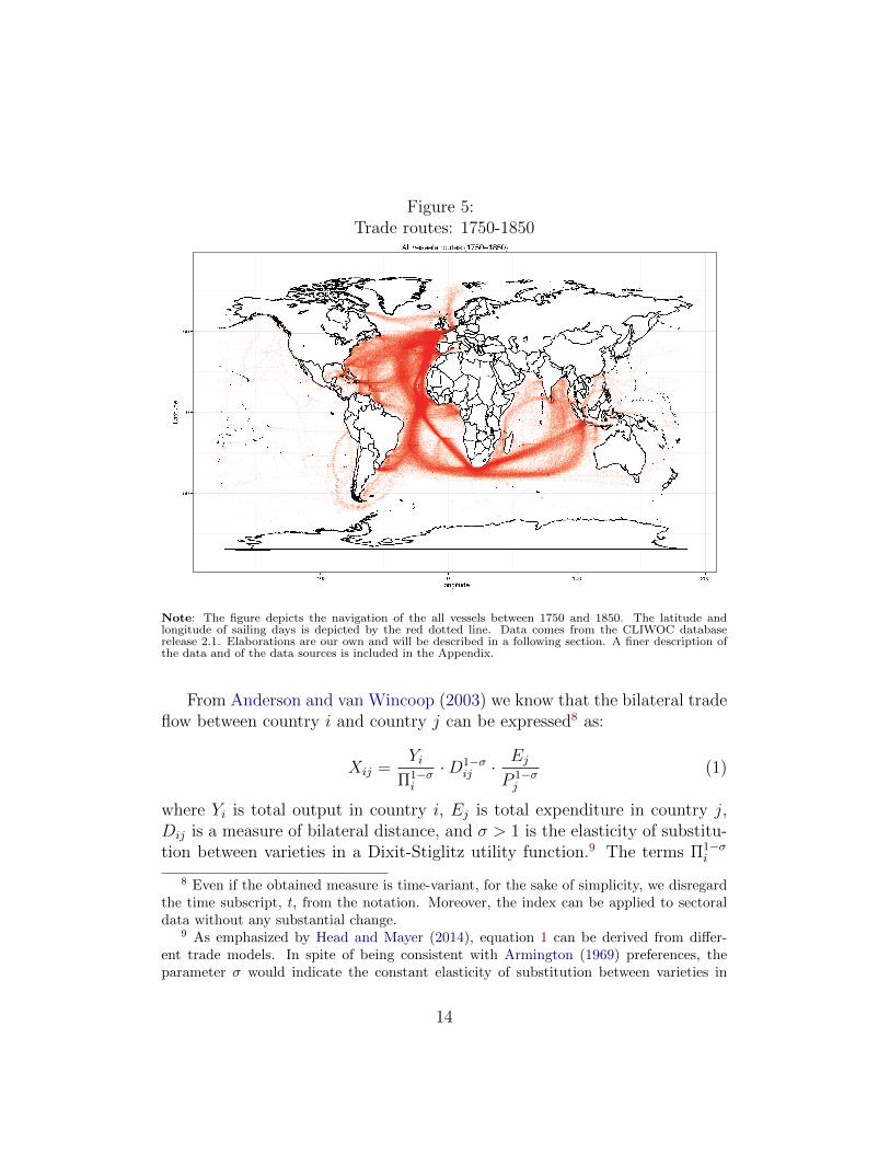
Figure 5:Trade routes: 1750-1850

Note: The figure depicts the navigation of the all vessels between 1750 and 1850. The latitude andlongitude of sailing days is depicted by the red dotted line. Data comes from the CLIWOC databaserelease 2.1. Elaborations are our own and will be described in a following section. A finer description ofthe data and of the data sources is included in the Appendix.

From Anderson and van Wincoop (2003) we know that the bilateral tradeflow between country i and country j can be expressed8 as:

Xij =Yi

Π1−σi

·D1−σij · Ej

P 1−σj

(1)

where Yi is total output in country i, Ej is total expenditure in country j,Dij is a measure of bilateral distance, and σ > 1 is the elasticity of substitu-tion between varieties in a Dixit-Stiglitz utility function.9 The terms Π1−σ

i

8 Even if the obtained measure is time-variant, for the sake of simplicity, we disregardthe time subscript, t, from the notation. Moreover, the index can be applied to sectoraldata without any substantial change.

9 As emphasized by Head and Mayer (2014), equation 1 can be derived from differ-ent trade models. In spite of being consistent with Armington (1969) preferences, theparameter σ would indicate the constant elasticity of substitution between varieties in

14

and P 1−σj are the“inward” and “outward” multilateral resistance terms, cap-

turing the interconnectedness among countries that is revealed through theprice index in the importing market, P 1−σ

j , and through the price index Π1−σi

capturing the degree of competition faced by the exporting country. SinceAnderson and van Wincoop (2003), the multilateral resistance terms high-light the fundamental relevance of considering distance in relative terms, andnot only in absolute terms, as expressed by Dij.

Being σ the elasticity of substitution among product varieties, the va-rieties considered in the expenditure function of consumers must necessaryinclude both domestic varieties and foreign varieties. Accordingly, the gravityequation (1) should consider not only foreign trade but also domestic trade,Xii and Xjj.

10 On that we follow Jacks et al. (2008), Chen and Novy (2012)and Novy (2013).

Being N the total number of countries, for consistency we must have that:

Yi ≡N−1∑i 6=j

Xij +Xii; (2)

Ej ≡N−1∑i 6=j

Xij +Xjj. (3)

Xii and Xjj are in general not observed and must be therefore estimatedor - as in our case - can be calculated using equation (2) and (3).

Replacing the missing domestic trade with the calculated one, the tradematrix Xij will now be a N ×N matrix with domestic trade along the maindiagonal, instead of the usual case of a N×(N−1) matrix, as it is commonly

a monopolistic competition trade models a la Krugman. In Melitz (2003) and Chaney(2008) the same parameter refers to the exponent of the Pareto distribution of firms’productivity (the higher σ the less would be the productivity dispersion among firms).Finally, in Eaton and Kortum (2002) the parameter σ would indicate the exponent of theFrechet distribution defining the countries’ productivity across product varieties. See alsoDe Benedictis and Taglioni (2011) on this point.

10 The domestic trade component is usually disregarded in gravity models, making themodel inconsistent with the data. Wei (1996) derives domestic trade in order to derive thenotion of home bias from a microfounded gravity equation. According to his definition:“ . . . a country’s home bias . . . [is the] imports from itself in excess of what it wouldhave imported from an otherwise identical foreign country (with same size, distance andremoteness measure).” See also Wolf (2000) on that.

15

used. When Xii and Xjj are included in the trade matrix, Jacks et al. (2008)show that:

τij =

(XiiXjj

XijXji

) 12(σ−1)

− 1 (4)

Using this indirect approach of measuring trade costs, we obtain the compre-hensive aggregate measure of bilateral trade costs τij. As shown by Chen andNovy (2011), this trade cost index is the geometric average of internationaltrade costs between countries i and j relative to domestic trade costs withineach country.11

Intuitively, when countries trade more internationally than they do do-mestically that gets reflected in low trade costs, that will be high in theopposite case. The benchmark case, that is usually taken as a lower boundfor τij, is when in both countries total output is equally traded inside andoutside the country. In that event τij = 0 for all level of σ.12 As the ratioin equation 4 rises above one, with countries trading more domestically thaninternationally, international trade costs rise relative to domestic trade costs,and τij takes positive values that reach the upper bound of the index, whencountries do not trade internationally and τij = +∞.

Since the index is a product of the two countries trade flows, the levelof trade of one country influences the trade cost of the other country at thebilateral level. In this respect, τij is a symmetric measure of bilateral tradecosts.

4.1 Descriptives

Following the methodology proposed by Jacks et al. (2008), and further dis-cussed in Chen and Novy (2011), Chen and Novy (2012) and Novy (2013),we calculate a comprehensive measure of bilateral trade cost, τij, as in equa-

11 A similar measure of freeness of trade (or phi -ness) as been proposed by Head andRies (2001) and Head and Mayer (2004), where φij is an overall trade cost indirectlycapturing the bundle of variables influencing trade cost, scaled by σ. See also Chen andNovy (2012) for some important details that make τij different from φij .

12 When in the hypothetical case the domestic trade of one of the two countries is null,

the ratioXiiXjj

XijXji> 1, and for a given σ, τij = −1. The events in which this happens

in the data used are none. The Appendix 9.4 contains descriptive statistics on the thedistribution of τij and on some limited cases of unusual behavior of the index.

16

tion 4, for 191 countries and 18145 country pairs. We used bilateral tradedata from the Cepii revision of the Comtrade UN database to derive theaggregate measure of bilateral trade xij, and we calculate internal trade xiiusing data on GDP reported in the World Bank WDI dataset. As far as σwe use estimates from the literature on trade elasticity (Eaton and Kortum,2002, Anderson and Yotov, 2012), mainly working with a σ = 11, but alsolowering the level of σ to 9 or 7 to check for the robustness of the results.

Even if it is possible to calculate such measure for every year between1995 and 2010, we will exploit the time dimension of trade costs only inthe descriptive analysis, while in the inferential part of the paper, since thegeographic dimension of the data is time invariant, we will concentrate onthe cross-country variability of τij.

4.1.1 Trade and trade costs

In figure 6 we plot the chronological evolution of world exports between 1995and 2010, measured in natural logarithms (left panel,) and the respectivetrade costs, measured by τij. In the time span covered by the analysis, worldexports evolve according to three phases: the first one of relatively moderategrowth (1995-2002), the second one of acceleration (2003-2007), and the lastphase of the Great Trade Collapse and its recovery (2008-2010).

During the first phase average international trade costs reduced sharply,moving from a proportion of 4.4:1 with domestic trade costs to a much mod-erate 3.75. In the subsequent phases the average τij went up and down insidethe band between 3.5 and 3.8. Even during the recent period of trade con-traction, average trade cost increased, by no means, but not as dramaticallyas one could have imagined.

4.1.2 The distribution of trade costs

Figures 7 illustrates the frequency distributions of the log transformation ofτij for 1995 and 2000. The kernel densities clearly show a trimodal empiricaldistribution with a different balance between the low, medium and high val-ues of trade costs. Averages across the all periods reveal a neat heterogeneityin trade costs when looking at countries all together. Striking differences ap-pear across level of insularity. Landlocked countries and Islands show higherlevel of trade costs, and a prevalent right mode; in Coastal and, especially, inPartial Island countries the right mode is less accentuated. This last group

17

Figure 6:

Trade and trade costs: 1995-2010

2929

.530

30.5

log

of w

orld

exp

orts

1995 2000 2005 2010year

3.6

3.8

44.

24.

4A

vera

ge W

orld

Tra

de C

osts

1995 2000 2005 2010year

Note: The figure traces the time series of world exports (left panel, measured in natural logarithms) andtrade costs (right panel,) as measured in equation 4 with σ = 11 and zero-trade flows replaced by xij = 1.Data comes from the BACI-CEPII database and the World Bank. Elaborations are our own. Furtherdescription of the data and of the data sources is included in the Appendix.

of countries is remarkably characterized by very low τij. Country pairs withminimal trade costs are however present in all groups of countries, as shownby the left outliers in the levels of τij visualized by the dots at the basisof the kernel densities. What is also remarkable is that the changes in τijoccurring between 1995 and 2000 appear to be more relevant in Coastal andLandlocked countries, much less so in Island countries, especially in terms ofhigh levels of trade costs.

4.1.3 Trade Costs and Insularity

To further explore the relationship between trade costs and insularity, wereport in figure 8 a spatial scatter plot having longitude on the horizontalaxis and latitude on the vertical axis, as in a cartogram, and where countries,identified by ISO3 codes, are located according to the latitude and longitudeof countries capital cities. The countries dots are differentiated according tothe color corresponding to the four level of the Insularity index previously de-scribed (black=landlocked; green=coastal; blue=partial island; red=island).The dimension of the dot is proportional to the level of the average countryτij in 2010, with σ = 11, in logs.13

Among the 191 countries included in the dataset, 32 are Landlocked, 88

13 See also the 3D version of this scatterplot (including a nonparametric surface visual-izing estimated trade costs) and the related heatmap included in the Appendix.

18

Figure 7:

Kernel density of trade costs: Country pairs averages 1995-2010

Note: Our elaborations on BACI-CEPII data and the World Bank WDI data. τij is computed accordingto equation 4 with σ = 11, and zero-trade flows replaced by xij = 1. The smoothing parameter of thekernel function is set optimally. The red empirical distributions corresponds to the year 2010, while theorange one to 1995. The spikes aligned below the kernel densities depict the position of each observation.

are Costal, 17 are Partial Islands and 54 are Islands. In this latter group, asfor the others, we have countries with very high average bilateral trade costs,such as Tonga (TON), and countries with low average bilateral trade costs,such as the United Kingdom (GBR) or Singapore (SGP). In general, high orlow trade costs do not seem to be a peculiar feature of any specific group ofcountries in the Insularity index.

19

Figure 8:

Spatial scatter plot: trade costs (2010) and insularity

ABW

AFG

AGO

ALB

ARE

ARG

ARM

ATG

AUS

AUT

AZE

BDI

BEN

BFA

BGD

BGR

BHRBHS

BIH

BLRBLX

BLZ

BMU

BOL

BRA

BRB

BRN

BTN

CAF

CANCHE

CHL

CHN

CIVCMR

COG

COL

COM

CPV

CRI

CUB

CYM

CYP

CZEDEU

DJI

DMA

DNK

DOM

DZA

ECU

EGY

ERI

ESP

EST

ETH

FIN

FJI

FRA

FSM

GAB

GBR

GEO

GHA

GIN

GMBGNB

GNQ

GRC

GRD

GRL

GTM

GUY

HKG

HND

HRV

HTI

HUN

IDN

IND

IRL

IRNIRQ

ISL

ISR

ITA

JAM

JOR

JPN

KAZ

KEN

KGZ

KHM

KIR

KNA

KOR

KWT

LAO

LBN

LBR

LBY

LCA

LKA

LTULVA

MAC

MAR

MDA

MDG

MDV

MEX

MHL

MKD

MLI

MLT

MMR

MNG

MNP

MOZ

MRT

MUS

MWI

MYS

NCL

NER

NGANIC

NLD

NOR

NPL

NZL

OMN

PAK

PAN

PER

PHL

PLW

PNG

POL

PRKPRT

PRY

PYF

QAT

ROM

RUS

RWA

SAU

SDNSEN

SGP

SLB

SLE

SLV

SMR

SOMSTP

SUR

SVKSVN

SWE

SYC

SYR

TCA

TCD

TGO

THA

TJKTKM

TMP

TON

TTO

TUN

TUR

TUVTZA

UGA

UKR

URY

USAUZB

VCTVEN

VNM

VUT

WSM

YEM

ZAF

ZAR

ZMBZWE

−25

0

25

50

−100 0 100Longitude

Latit

ude

trade.costs

−0.5

0.0

0.5

1.0

1.5

2.0

Insularity index

costal

island

landlocked

partial island

Insularity and trade costs

Note: Our elaborations on BACI-CEPII data and the World Bank WDI data. τij is computed accordingto equation 4 with σ = 11, and zero-trade flows replaced by xij = 1. Dots are colored according to thedifferent levels of the insularity index. The size of the dots is proportional to average country τij in 2010.

Figure 9 uses the same data, measuring bilateral distance on the horizon-tal axis, and average bilateral trade costs on the vertical axis. Every countryi is therefore identified by a couple of values, the first one is the averagebilateral distance between country i and every trading partner j, the secondone is the average bilateral trade cost (in logs) in 2010, between i and itstrade partners. Countries are identified by Iso3 codes and dots are coloredaccording to levels of the Insularity index, as in figure 8. In this case, to giveevidence to the variability of bilateral trade cost for every country i, the sizeof the dots is made proportional to the standard deviation of the country τijin 2010.

Let’s take Italy (ITA) as an example, the country has low average bilat-eral trade costs and also a low standard deviation of τij, but it trades withcountries located at a low average distance. Taking the United States (USA)as a comparison, the two moments of the distribution of bilateral trade costsare quite similar but the US trades on average with partners with are at ahigher distance with respect to the ones of Italy.

20

Figure 9:

Distance and trade costs scatter plot (2010)

ABWAGO

ALB

ARE

ARG

ARMATG

AUS

AUT

AZE

BDI

BENBFA

BGD

BGR

BHR

BHS

BIH

BLR

BLX

BLZ

BMU

BOL

BRA

BRB

BRN

BTN

CAF

CAN

CHE

CHL

CHN

CIV

CMRCOG

COL

COMCPV

CRI

CUB

CYP

CZE

DEU

DJI

DMA

DNK

DOM

DZA

ECU

EGY

ERI

ESP

EST

ETH

FIN

FJI

FRA

FSM

GAB

GBR

GEO

GHA

GIN

GMB

GNBGNQ

GRC

GRD

GRL

GTM

GUY

HKG

HND

HRV

HTI

HUN

IDN

IND

IRL

IRN

IRQ

ISL

ISR

ITA

JAM

JOR

JPN

KAZKEN

KGZKHM

KIR

KNA

KOR

KWT

LAO

LBN

LBR

LBYLCA

LKA

LTU

LVA

MAC

MAR

MDAMDG

MDV

MEX

MHL

MKD MLI

MLT

MNG

MOZ

MRT

MUS

MWI

MYS

NCL

NER

NGA

NIC

NLD

NOR

NPL

NZL

OMN PAKPAN

PER

PHL

PLW

PNG

POL

PRT

PRY

PYF

QAT

ROM

RUS

RWA

SAU

SDN SEN

SGP

SLB

SLE

SLV

SMR

SUR

SVK

SVN

SWE

SYC

SYR

TCD

TGO

THA

TJK

TKM

TMP

TON

TTO

TUN

TUR

TUV

TZA

UGA

UKR

URY

USA

UZBVCT

VENVNM

VUTWSM

YEM

ZAF

ZAR

ZMBZWE

0

1

2

8.50 8.75 9.00 9.25 9.50Average bilateral distance

Log

trad

e co

sts

Standard deviation of trade costs

0.5

1.0

Insularity index

costal

island

landlocked

partial island

Insularity, trade costs (moments) and distance (2000)

Note: Our elaborations on BACI-CEPII data and the World Bank WDI data. τij is computed accordingto equation 4 with σ = 11, and zero-trade flows replaced by xij = 1. Countries are identified by Iso3codes. Dots are colored according to the different levels of the insularity index. The size of the dots isproportional to the standard deviation of the country τij in 2010.

The general tendency is of a positive correlation between distance andtrade costs. This tendency is accentuated for landlocked countries and is-lands, less so for coastal countries. Variability of τij, measured by its stan-dard deviation is substantially unrelated with distance. Finally, islands canbe roughly divided in two groups for each variable of interest: in terms oftrade costs, figure 9 shows a prevalence of islands with high τij, but also asubstantial number of islands with low τij (i.e. Singapore (SGP)); in termsof average bilateral distance, the islands in the Pacific Ocean are all charac-terized by trade with countries located at a very high distance, while islandin the Atlantic Ocean are not. European islands form a third separate group.As a side evidence, large islands (such as Australia (AUS), Indonesia (IDN),Japan (JAP), and the United Kingdom (GBR)) are associated with low tradecosts. We will return to this issue later on.

21

4.1.4 Trade Costs and distance: Some European examples

Let’s now have a look at some specific country cases. We focus, as an exam-ple, on some European countries, with the twofold goal of illustrating howtrade costs are related to distance to foreign markets but that they cannot befully assimilated to distance, and that islands are different from other coun-tries’ geographical conditions in terms of how distance is related to tradecosts.

Figure 10 gives evidence of the relation between distance to Europeanmarkets and 1995-2010 average trade costs for four European countries:Cyprus, France, Germany, and the UK.

In general, at least for the three continental countries a some how positivecorrelation between distance and trade costs exists. However, in all cases thehighest bilateral trade costs are with Albania (ALB), even if for none of thefour countries Albania represents the European foreign market farther away.For France, Germany and the UK the trade partnership with Cyprus is theone that implies the longest distance, as far as intra-European trade.

Two elements seems to characterize an island like Cyprus. First of all,trade costs reach higher levels with respect to the ones of the three conti-nental countries. Secondly, the relationship between trade costs and distancedoesn’t seem to follow a linear path, but shows an inverted-U shape. Inter-mediate levels of distance show higher trade costs, and Italy (ITA), which isaround 2000 Kms away from Cyprus, and the Netherlands (NLD,) which is3000 Kms away from Cyprus, show the same level of bilateral trade costs.

It is useful to summarize the evidence so far. Islands seem to be differentfrom other countries in terms of trade costs. The spatial discontinuity withforeign countries add a further burden. On the other hand, islands are notall similar. What makes them different from each others?

4.1.5 Further geographical covariates

The first hypothesis is that islands are characterized by geographical speci-ficities - apart being an island - that are different from the ones of othercountries. The denomination of “island” could, therefore, hide some relevantgeographical dimension that could explain why “islands” look so different intheir trade costs.

The geographical dimensions that we consider and that we use as covari-ates in the empirical model described in section 5.

22

Figure 10:

Trade Costs and distance: Some European cases

ALB

AUT

BLX

BIH

BGR

BLR

HRVCZE DNKESTFINFRA

DEU

GRC

HUN

ISL

IRLITA

LVALTU

MLT

MDA

NLD

NORPOL

PRT

ROM

SVKSVNESPSWE

CHE

TUR UKR

MKD

GBR

.51

1.5

2A

vera

ge T

C a

cros

s E

U d

estin

atio

ns

0 1500 3000 4500Distance (km)

CyprusALB

AUT

BLX

BIH

BGR

BLR

HRV

CYP

CZEDNK

EST

FIN

DEU

GRC

HUN

ISL

IRLITA

LVA

LTU

MLT

MDA

NLD

NORPOLPRT

ROMSVKSVN

ESP

SWECHE

TUR

UKR

MKD

GBR

.2.4

.6.8

11.

2A

vera

ge T

Cs

acro

ss E

U d

estin

atio

ns

0 1500 3000 4500Distance (km)

France

ALB

AUTBLX

BIH

BGRBLR

HRV

CYP

CZE

DNK

EST

FIN

FRA

GRC

HUN

ISL

IRLITA

LVALTU MLT

MDA

NLD

NORPOL

PRTROM

SVKSVN ESPSWE

CHE

TUR

UKRMKD

GBR

.2.4

.6.8

11.

2A

vera

ge T

C a

cros

s E

U d

estin

atio

ns

0 1500 3000 4500Distance (km)

GermanyALB

AUT

BLX

BIH

BGRBLRHRV

CYPCZEDNK

ESTFIN

FRADEU

GRCHUN

ISL

IRL

ITA

LVALTUMLT

MDA

NLDNOR

POLPRTROMSVKSVN

ESPSWECHETUR

UKRMKD

0.5

11.

5A

vera

ge T

C a

cros

s E

U d

estin

atio

ns

0 1500 3000 4500Distance (km)

UK

Note: The figure includes the scatterplots for Cyprus, France, Germany and the UK depicting the relationbetween distance to European markets (horizontal axis) and 1995-2010 average trade costs (vertical axis).Countries are identified by their ISO3 UN codes. Data comes from the CEPII database. Elaborations areour own. Further description of the data and of the data sources is included in the Appendix.

Figure 11: Simple correlation among covariates

Island-states Rugged Distance to coast Tropical Avg. temperature Avg. precipitation Distance from EquatorRugged 1Distance to coast -0.1664* 1Tropical -0.0158* -0.3521* 1Avg. temperature -0.0034 -0.7283* 0.6039* 1Avg. precipitation -0.0395* -0.2717* 0.6282* 0.3301* 1Distance from Equator -0.0548* 0.5471* -0.7458* -0.8924* -0.4757* 1

Landlocked Rugged Distance to coast Tropical Avg. temperature Avg. precipitation Distance from EquatorRugged 1Distance to coast -0.2740* 1Tropical -0.3306* 0.0216* 1Avg. temperature -0.5440* -0.0205* 0.6455* 1Avg. precipitation 0.4324* -0.5029* 0.5383* 0.1451* 1Distance from Equator 0.1934* -0.0256* -0.7777* -0.8394* -0.3895* 1

Partial-insularity Rugged Distance to coast Tropical Avg. temperature Avg. precipitation Distance from EquatorRugged 1Distance to coast -0.2098* 1Tropical -0.2862* -0.1500* 1Avg. temperature 0.0410* -0.6513* 0.5966* 1Avg. precipitation 0.0601* -0.2656* 0.7440* 0.5873* 1Distance from Equator -0.0869* 0.4027* -0.7906* -0.8663* -0.7405* 1

Note: Further description of the data and of the data sources is included in the Appendix.

23

4.1.6 Connectedness

It’s now time to go back to John Donne Meditation. Islands are not alwaysseverely isolated, some times for some of them is easier to be “. . . a peece ofthe Continent, a part of the main . . . ”. Geographical proximity with themainland is probably the first candidate to explore in order to evaluate howconnectedness with foreign countries can reduce the onus of islands bilateraltrade costs.

A way to represent the relevance of spacial connectedness is the one thatchanges the visual perspective of the adjacency between countries takingspace (latitude and longitude) in the background. This perspective is offeredby a network visualization of countries proximity, as represented in figure 14.

The figure visualizes the spatial connectedness between countries, iden-tified by their Iso3 codes. Countries that share a common land border areconnected by a link;14 light blue nodes are islands, yellow nodes are main-land countries. The nodes with a black thick circle around are landlockedcounties, while nodes with a red circle are partial islands (PP), as defined insection 2.2. The position of each node depends on its relative spacial connect-edness as obtained through the use of a “brute force algorithm” for networkvisualization.15 Islands are located near the closer country according to theintervals ≤300 Kms, and ≤500 Kms.

The spatial network is characterized by a giant component of directly andindirectly connected nodes and by a second component made of countries ofthe Americas. The majority of islands are isolates, while some of them (e.gthe United Kingdom and Ireland (IRL), or the Dominican Republic (DOM)and Haiti (HTI)) are locally connected.

Landlocked countries are located inside the network component. Some ofthem show a high level of centrality (e.g. Niger (NER) and Mali (MLI), orHungary (HUN) and Austria (AUT)). Partial islands play the role of gate-keepers and are located at the boundaries of the network components. Theposition of islands in the topology of the spatial network depends on nearby

14 The length of the link is endogenously determined by the visualization algorithm andhas no specific meaning. The adjacency matrix that corresponds to the network in figure14 is a binary matrix. Only two alternatives are considered: sharing or not sharing aland border. Pakistan (PAK) and India (IND) share a common land border, as India andBangladesh (BGD). The difference in the length of the two different links is due to thegeneral effect of global adjacency (e.g. Pakistan is linked also to Iran (IRN) that is notlinked to India, and that drives India and Pakistan far apart.

15 The algorithm used is the Kamada Kawai algorithm.

24

Figure 12:

A network visualization of countries’ spatial connectedness

ABW

AFG

AGO

ALB

ARE

ARG

ARM

ATG

AUS

AUT

AZE

BDI

BEN

BFA

BGD

BGR

BHR

BHS

BIH

BLR

BLX

BLZ

BMU

BOL

BRABRB

BRN

BTN

CAF

CAN

CHE

CHL

CHN

CIV

CMR

COG

COL

COM

CPV

CRI

CUB

CYMCYP

CZE

DEU

DJI

DMA

DNK

DOM

DZA

ECU

EGY

ERI

ESP

EST

ETH

FIN

FJI

FRA

FSM

GAB

GBR

GEO

GHA

GIN

GMB

GNB

GNQ

GRC

GRD

GRL

GTM

GUY

HKG

HND

HRV

HTI

HUN

IDN

IND

IRL

IRN

IRQ

ISL

ISR

ITA

JAM

JOR

JPN

KAZ

KEN

KGZ

KHM

KIR

KNA

KOR

KWT

LAO

LBN

LBR

LBY

LCA

LKA

LTULVA

MAC

MAR

MDA

MDG

MDV

MEX

MHL

MKD

MLI

MLT

MMR

MNG

MNP

MOZ

MRT

MUS

MWI

MYS

NCL

NER

NGA

NIC

NLD

NOR

NPL

NZL

OMN

PAK

PAN

PER

PHL

PLW

PNG

POLPRK

PRT

PRY

PYF

QAT

ROM

RUS

RWA

SAU

SDN

SEN

SGP

SLB

SLE

SLV

SMR

SOM

STP

SUR

SVK

SVN

SWE

SYC

SYR

TCA

TCD

TGO

THA

TJK

TKM

TMP

TON

TTO

TUN

TUR

TUV

TZA

UGA

UKRURY

USA

UZB

VCT

VEN

VNMVUT

WSM

YEM

ZAF

ZAR

ZMB

ZWE

Note: The figure represents spatial connectedness between countries. Links connect countries that sharea common border; light blue nodes are islands, yellow nodes are mainland countries. The nodes with ablack thick circle around are landlocked counties, while nodes with a red circle are partial islands (PP) asdefined in section 2.2. The position of each node depends on its relative connectedness as in the KamadaKawai algorithm for network visualization. Islands are located near the closer country according to theintervals ≤300 Kms, and ≤500 Kms. Data comes from the CEPII database. Elaborations are our own.Further description of the data and of the data sources is included in the Appendix.

countries. The United Kingdom has a central role in the networks, whileMicronesia (FSM) is quite isolated. But the topology of the spatial networkreveals an important element of the relative spatial position of countries: trueisolation is rare and countries, even islands, should be considered as “partsof the main”.

To capture spatial connectedness we define a nested index that progres-sively consider countries according to their level of spatial proximity. At thefirst level the index takes a value of one if the two countries i and j sharea common land border; at the second level the index adds in the countrieswhich bilateral distance is below the limit of 300 Kms; at the third level theindex includes also the countries which bilateral distance is below the limit

25

of 500 Kms. All remaining country pairs are given a value of zero.The index will be used in subsequent regressions to control for the role

of spatial connectedness in influencing trade costs.

5 The empirical model

While the recent literature on calculated trade costs measures (Chen andNovy (2011) and Novy (2013)) has been motivated to delve trade costs overtime along with factors which have been driving their evolution, the startingmodel equation is the standard trade costs function as in Anderson and Yotov(2012):

τijt = exp(αDij +Xijtγ) + εijt (5)

where the dependent variable is calculated as in 4; Dij is the standard mea-sure of distance and Xijt is the matrix of geographical covariates, discussedin section 4.1.5.

In this paper we use the same methodology as in Novy (2013) to investi-gate the variance of trade costs in space, i.e. across countries, instead of itstime variation. We modify the estimated equation accordingly, in order toadapt it to our variance analysis where correlates are time invariant. There-fore in our model the dependent variable is an average of τij across the years(1995-2010) regressed against measures of the geography of a country eitherin its exporter of importer position (i or j). Controls for the heterogeneity ofthe pairs are captured by a random effect term, θij, and the multilevel ran-dom effect modelling allows us to estimate coefficients for the time invariantterms we are interested in, including a control for the variance in trade costsacross pairs. Our simple model looks like:

lnτij = β1Iij + β2Ibothij + β3LLij + β4LLbothij + β5PIij + β6PIbothij+

+αlnDij + lnXijγ + θij + εij(6)

where θij is the random component of the error term, with E(θ = 0) andvariance constant for the pair; and εij is a standard idiosyncratic error, clus-tered at the country-pair level. Using the same symbol as in the Insularitytaxonomy, I is a dummy equal to 1 if one of the two countries in the pair

26

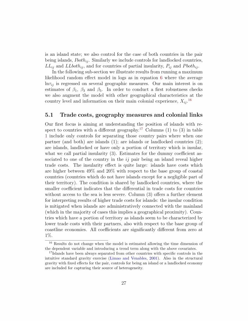
is an island state; we also control for the case of both countries in the pairbeing islands, Ibothij. Similarly we include controls for landlocked countries,LLij and LLbothij, and for countries of partial insularity, Pij and Pbothij.

In the following sub-section we illustrate results from running a maximumlikelihood random effect model in logs as in equation 6 where the averagelnτij is regressed on several geographic measures. Our main interest is onestimates of β1, β3 and β5. In order to conduct a first robustness checkswe also augment the model with other geographical characteristics at thecountry level and information on their main colonial experience, Xij.

16

5.1 Trade costs, geography measures and colonial links

Our first focus is aiming at understanding the position of islands with re-spect to countries with a different geography.17 Columns (1) to (3) in table1 include only controls for separating those country pairs where when onepartner (and both) are islands (1); are islands or landlocked countries (2);are islands, landlocked or have only a portion of territory which is insular,what we call partial insularity (3). Estimates for the dummy coefficient as-sociated to one of the country in the ij pair being an island reveal highertrade costs. The insularity effect is quite large: islands have costs whichare higher between 49% and 20% with respect to the base group of coastalcountries (countries which do not have islands except for a negligible part oftheir territory). The condition is shared by landlocked countries, where thesmaller coefficient indicates that the differential in trade costs for countrieswithout access to the sea is less severe. Column (3) offers a further elementfor interpreting results of higher trade costs for islands: the insular conditionis mitigated when islands are administratively connected with the mainland(which in the majority of cases this implies a geographical proximity). Coun-tries which have a portion of territory as islands seem to be characterized bylower trade costs with their partners, also with respect to the base group ofcoastline economies. All coefficients are significantly different from zero at1%.

16 Results do not change when the model is estimated allowing the time dimension ofthe dependent variable and introducing a trend term along with the above covariates.

17Islands have been always separated from other countries with specific controls in theintuitive standard gravity exercise (Limao and Venables, 2001). Also in the structuralgravity with fixed effects for the pair, controls for being an island or a landlocked economyare included for capturing their source of heterogeneity.

27

The term which captures those limited cases of both countries in the pairin the same geographical condition (both islands, both landlocked or bothpartial insular) suggest that having a two-sided (symmetric) geographicalcondition is more relevant for landlocked countries and also for those oneswhich are partially insular.

In columns (4) to (7) of table 1 we include further controls for testing therobustness of our significant and positive higher trade costs when an islandor a landlocked country is in the pair. First of all the size of a country.The fact of being small is a geographic characteristics which repeatedly theliterature has reported as a disadvantage condition (the main point beingthe limited possibility of exploiting diversification economies and to tap intoeconomies of scale). The fact of being a small island is the crucial conditionreported in the literature of development (see references as Easterly andKraay (2000)). Therefore it is our interest to dissect whether the effect we arecapturing can be attributed to the fact of being small.18 Results in column(4) suggest that size matters (smaller countries show higher trade costs)but also after controlling for it islands show higher trade costs than coastalcountries. In column (5) we control for distance and results show that givenfor a distance islands and landlocked countries have higher trade costs thancoastal countries while the result for countries which have islands is different.In columns (6) and (7) of table 1 measures of geography reported as robustcorrelates with income and trade are included: Nunn and Puga (2012) Puga’sruggedness index, standard variables reporting different climate zones in theplanet (percentage of tropical territory, precipitation, distance from equator,as in La Porta et al. (1997)) and the standard distance from coast (see DataInfo in 9). Results on our augmented models are consistent with expectationof bad geography conditions to be associated to higher trade costs. We do notreport changes in the coefficients linked to the insular condition but, notably,we report on the information that the variable distance from coast add toour previous results: the measure shows a perfect capture of the nature ofbeing landlocked. When we take it out (column 7) results come back to whatpreviously stated.

In column (8) we also reported the effects of including colonial ties con-

18 We included a geographical measure of size, land extension in km squared so that toavoid elements of endogeneity with trade costs. Of course we do not control in this wayfor any density effect, size in land does not implies size in population or income thoughtthis case is more evident for some countries with extensive land.

28

trols referred to several national-state empires.19 Results on our variables ofinterest do not change: insularity is associated with higher trade costs; thecase is replicated for landlocked countries, with a smaller size of the effect:landlocked countries have trade costs 16% higher than coastal countries; theeffect increases to 22% when islands states are in the pair. Higher trade costslinked to the insular condition highlight a crucial element of the islands’ geog-raphy: precluding the possibility of sharing the infrastructure of contiguousneighbours which are possibly better connected to the international markets.

19 Australian, Austrian, Belgian, German, Danish, Spanish, French, English, Italian,Japanese, Dutch, New Zealander, Portuguese, Russian, Turkish, American and Yugosla-vian

29

Tab

le1:

Tra

de

cost

sco

rrel

ates

(1)

(2)

(3)

(4)

(5)

(6)

(7)

(8)

VA

RIA

BL

ES

lnτ ij

lnτ ij

lnτ ij

lnτ ij

lnτ ij

lnτ ij

lnτ ij

lnτ ij

ISL

AN

D0.

402*

**0.

481*

**0.

429*

**0.

385*

**0.

209*

**0.

254*

**0.

215*

**0.

200*

**(0

.012

)(0

.012

)(0

.012

)(0

.012

)(0

.012

)(0

.012

)(0

.012

)(0

.013

)

BO

TH

ISL

AN

DS

0.01

740.

103*

**0.

0502

*0.

0061

00.

0421

*0.

0658

**0.

0302

0.03

81(0

.023

)(0

.023

)(0

.023

)(0

.022

)(0

.021

)(0

.022

)(0

.022

)(0

.020

)

LA

ND

LO

CK

ED

0.36

0***

0.30

8***

0.27

7***

0.26

7***

0.00

772

0.26

6***

0.14

6***

(0.0

13)

(0.0

13)

(0.0

13)

(0.0

12)

(0.0

15)

(0.0

12)

(0.0

16)

BO

TH

LA

ND

LO

CK

ED

0.24

5***

0.19

2***

0.16

0***

0.22

1***

-0.0

646*

0.19

5***

0.07

23*

(0.0

36)

(0.0

35)

(0.0

34)

(0.0

32)

(0.0

31)

(0.0

30)

(0.0

33)

PA

RT

IAL

INSU

LA

R-0

.321

***

-0.3

37**

*-0

.334

***

-0.1

54**

*-0

.192

***

-0.0

316*

(0.0

16)

(0.0

15)

(0.0

14)

(0.0

14)

(0.0

14)

(0.0

15)

BO

TH

PA

RT

IAL

INSU

LA

R-0

.244

***

-0.2

61**

*-0

.250

***

-0.0

521

-0.0

902

0.02

19(0

.065

)(0

.064

)(0

.059

)(0

.053

)(0

.055

)(0

.071

)

Lan

dA

rea

(100

0sq

uar

edkm

)-0

.060

2***

-0.0

686*

**-0

.101

***

-0.0

653*

**-0

.130

***

(0.0

02)

(0.0

02)

(0.0

02)

(0.0

02)

(0.0

03)

Log

ofsi

mple

dis

tance

0.35

8***

0.33

6***

0.34

4***

0.39

5***

(0.0

07)

(0.0

07)

(0.0

07)

(0.0

07)

Ter

rain

Rugg

ednes

sIn

dex

0.04

43**

*0.

0161

***

0.00

206

(0.0

04)

(0.0

04)

(0.0

04)

Per

centa

geT

ropic

alT

erri

tory

0.24

1***

0.31

5***

0.22

1***

(0.0

18)

(0.0

18)

(0.0

19)

Annual

aver

age

tem

per

ature

countr

y0.

0050

0***

-0.0

0830

***

0.01

35**

*(0

.001

)(0

.001

)(0

.001

)

Pre

cipit

atio

n(m

etre

s)-0

.155

***

-0.2

40**

*-0

.109

***

(0.0

08)

(0.0

08)

(0.0

08)

Dis

tance

countr

yfr

omeq

uat

or(L

aP

orta

1999

)-0

.562

***

-1.0

48**

*-0

.149

*(0

.060

)(0

.059

)(0

.065

)

Dis

tance

tonea

rest

ice-

free

coas

t(1

000

km

.)0.

470*

**0.

286*

**(0

.016

)(0

.018

)

Con

trol

sfo

rco

lonia

llinks

NO

NO

NO

NO

NO

NO

NO

YE

S

Con

stan

t0.

837*

**0.

672*

**0.

777*

**0.

899*

**-2

.150

***

-2.0

16**

*-0

.916

***

-3.0

15**

*(0

.008

)(0

.010

)(0

.011

)(0

.011

)(0

.060

)(0

.109

)(0

.105

)(0

.118

)O

bse

rvat

ions

3436

634

366

3436

634

366

3436

631

132

3113

222

642

Clu

ster

edij

stan

dar

der

rors

inpar

enth

eses

.**

*p<

0.01

,**

p<

0.05

,*

p<

0.1

Dep

enden

tva

riab

leis

Tra

de

Cos

tsm

easu

red

asin

equat

ion

4,w

ithσ

=11

and

repla

cem

ent

for

zero

s.R

efer

ence

cate

gory

for

Isla

nds,

Lan

dlo

cked

and

Par

tial

lyIn

sula

rco

untr

ies

are

Coa

stal

countr

ies.

30

Model

1M

odel

2M

odel

3M

odel

4M

odel

5M

odel

6M

odel

7M

odel

8M

odel

9M

odel

10M

odel

11M

odel

12

fact

or(d

.isl

.sta

te3)

10.4

017

0.4

814

0.4

294

0.3

334

0.3

639

0.3

335

0.2

992

0.3

111

0.3

165

0.3

428

0.3

337

0.1

751

(0.0

123)

(0.0

121)

(0.0

123)

(0.0

125)

(0.0

143)

(0.0

125)

(0.0

123)

(0.0

123)

(0.0

121)

(0.0

120)

(0.0

119)

(0.0

116)

fact

or(d

.isl

.sta

te3)

20.4

191

0.5

848

0.4

796

0.2

878

0.2

535

0.2

881

0.2

196

0.2

372

0.2

512

0.3

071

0.2

894

0.1

630

(0.0

222)

(0.0

227)

(0.0

232)

(0.0

232)

(0.0

371)

(0.0

233)

(0.0

230)

(0.0

241)

(0.0

238)

(0.0

242)

(0.0

241)

(0.0

218)

fact

or(l

andlo

cked

3)1

0.3

604

0.3

081

0.3

085

0.3

085

0.3

148

0.3

275

0.3

419

0.3

288

0.3

033

0.2

401

0.2

371

(0.0

126)

(0.0

127)

(0.0

124)

(0.0

124)

(0.0

124)

(0.0

121)

(0.0

121)

(0.0

120)

(0.0

121)

(0.0

123)

(0.0

115)

fact

or(l

andlo

cked

3)2

0.6

051

0.4

999

0.5

008

0.5

012

0.5

133

0.5

389

0.5

622

0.5

356

0.4

808

0.3

579

0.4

191

(0.0

362)

(0.0

365)

(0.0

371)

(0.0

372)

(0.0

372)

(0.0

364)

(0.0

356)

(0.0

354)

(0.0

349)

(0.0

347)

(0.0

300)

fact

or(d

.par

tial

.insu

l3)1

−0.3

206−

0.3

357−

0.3

367−

0.3

336−

0.3

118−

0.2

903−

0.2

728−

0.2

615−

0.2

493−

0.2

505

(0.0

160)

(0.0

155)

(0.0

155)

(0.0

155)

(0.0

152)

(0.0

153)

(0.0

150)

(0.0

148)

(0.0

148)

(0.0

141)

fact

or(d

.par

tial

.insu

l3)2

−0.5

650−

0.5

952−

0.5

992−

0.5

909−

0.5

473−

0.5

033−

0.4

696−

0.4

424−

0.4

198−

0.4

131

(0.0

602)

(0.0

585)

(0.0

583)

(0.0

582)

(0.0

561)

(0.0

563)

(0.0

544)

(0.0

534)

(0.0

537)

(0.0

528)

ln.lan

dar

ea.i

−0.0

532−

0.0

608−

0.0

537−

0.0

412−

0.0

346−

0.0

450−

0.0

486−

0.0

600−

0.0

724

(0.0

014)

(0.0

027)

(0.0

014)

(0.0

015)

(0.0

016)

(0.0

017)

(0.0

019)

(0.0

020)

(0.0

018)

fact

or(d

.isl

.sta

te3)

1:ln

.lan

dar

ea.i

0.0

131

(0.0

032)

fact

or(d

.isl

.sta

te3)

2:ln

.lan

dar

ea.i

−0.

0014

(0.0

057)

rugg

ed.i

−0.0

155

0.0

087

0.0

215

0.0

338

0.00

320.0

206

0.0

211

(0.0

033)

(0.0

034)

(0.0

036)

(0.0

036)

(0.0

040)

(0.0

041)

(0.0

038)

trop

ical

.i.s

c0.2

844

0.1

199

0.3

966

0.2

243

0.1

997

0.2

627

(0.0

098)

(0.0

120)

(0.0

175)

(0.0

195)

(0.0

195)

(0.0

183)

avg.

tem

p.i

0.0

135

0.0

105

−0.0

117

0.00

04−

0.00

04(0.0

007)

(0.0

007)

(0.0

013)

(0.0

015)

(0.0

014)

pre

c.i.sc

−0.1

792−

0.2

064−

0.1

467−

0.2

227

(0.0

081)

(0.0

084)

(0.0

089)

(0.0

084)

dis

t.eq

LA

PO

RT

A.i

−1.3

987−

0.9

056−

0.7

731

(0.0

641)

(0.0

706)

(0.0

669)

dis

t.co

ast.

i0.2

749

0.2

403

(0.0

134)

(0.0

122)

lndis

t0.3

461

(0.0

073)

R2

0.06

450.

1127

0.13

640.

1650

0.16

550.

1655

0.18

730.

1883

0.19

920.

2089

0.21

740.

3184

Adj.

R2

0.06

440.

1126

0.13

620.

1648

0.16

520.

1653

0.18

710.

1880

0.19

890.

2086

0.21

710.

3181

Num

.ob

s.34

366

3436

634

366

3436

634

366

3436

634

366

3345

333

268

3271

532

715

3271

5

Coeffi

cien

tsw

ithp<

0.0

5in

bold

.

Tab

le2:

Tra

de

cost

s:is

lands

and

corr

elat

es.

31

Model

1M

odel

2R

aja

n-Z

inga

les

typ

em

odel

fact

or(d

.isl

.sta

te3)

10.1

751

0.1

751

0.1

652

(0.0

116)

(0.0

116)

(0.0

117)

fact

or(d

.isl

.sta

te3)

20.1

630

0.1

630

0.1

677

(0.0

218)

(0.0

218)

(0.0

223)

fact

or(l

andlo

cked

3)1

0.2

371

0.2

371

0.2

371

(0.0

115)

(0.0

115)

(0.0

115)

fact

or(l

andlo

cked

3)2

0.4

191

0.4

191

0.4

805

(0.0

300)

(0.0

300)

(0.0

295)

fact

or(d

.par

tial

.insu

l3)1

−0.2

505−

0.2

505

−0.2

571

(0.0

141)

(0.0

141)

(0.0

140)

fact

or(d

.par

tial

.insu

l3)2

−0.4

131−

0.4

131

−0.4

494

(0.0

528)

(0.0

528)

(0.0

555)

ln.lan

dar

ea.i

−0.0

724−

0.0

724

−0.0

730

(0.0

018)

(0.0

018)

(0.0

018)

rugg

ed.i

0.0

211

0.0

211

0.0

209

(0.0

038)

(0.0

038)

(0.0

038)

trop

ical

.i.s

c0.2

627

0.2

627

0.2

550

(0.0

183)

(0.0

183)

(0.0

183)

avg.

tem

p.i

−0.

0004

−0.

0004

−0.

0012

(0.0

014)

(0.0

014)

(0.0

014)

pre

c.i.sc

−0.2

227−

0.2

227

−0.2

219

(0.0

084)

(0.0

084)

(0.0

084)

dis

t.eq

LA

PO

RT

A.i

−0.7

731−

0.7

731

−0.8

309

(0.0

669)

(0.0

669)

(0.0

672)

dis

t.co

ast.

i0.2

403

0.2

403

0.2

389

(0.0

122)

(0.0

122)

(0.0

122)

lndis

t0.3

461

(0.0

073)

lndis

t.s

0.3

461

0.2

879

(0.0

073)

(0.0

133)

fact

or(d

.isl

.sta

te3)

1:ln

dis

t.s

0.1

265

(0.0

166)

fact

or(d

.isl

.sta

te3)

2:ln

dis

t.s

0.0

815

(0.0

241)

lndis

t.s:

fact

or(l

andlo

cked

3)1

0.0

768

(0.0

153)

lndis

t.s:

fact

or(l

andlo

cked

3)2

0.1

972

(0.0

382)

lndis

t.s:

fact

or(d

.par

tial

.insu

l3)1

−0.0

721

(0.0

192)

lndis

t.s:

fact

or(d

.par

tial

.insu

l3)2

−0.1

038

(0.0

467)

R2

0.31

840.

3184

0.32

38A

dj.

R2

0.31

810.

3181

0.32

33N

um

.ob

s.32

715

3271

532

715

Coeffi

cien

tsw

ithp<

0.0

5in

bold

.

Tab

le3:

Tra

de

cost

s:is

lands

and

dis

tance

32

5.2 Trade Costs, bad geography and connectedness

What makes islands different from other territories? Islands are surroundedby sea, which is the opposite of the crucial characteristic which makes the ge-ography of landlocked countries highly difficult. But sharing a border bringsadvantages. Adjacency favours exchanges through different channels most oftime built thought historical passages (what results in what we call and mea-sure as cultural openness). The way we address adjacency is directly linkedto measures which capture the non-linear effect of distance on exchanges. Inthis part of the analysis we try to capture some of this reasoning by interact-ing our insularity measure with measures of contiguity which are adjustedfor the spatial discontinuity generated by the sea.

lnτij = (β1Iij + β2Ibothij + β3LLij + β4LLbothij + β5PIij + β6PIbothij)

(σSCij + lnXijγ + θij + εij)

(7)

where SCij is an index that progressively consider countries according totheir level of spatial proximity in a nested structure. SCij at the first levelis equal to 1 if the two countries i and j share a common land border; at thesecond level the index adds in the countries which bilateral distance is belowthe limit of 300 Kms; at the third level the index includes also the countrieswhich bilateral distance is below the limit of 500 Kms. All remaining countrypairs are given a value of zero.

All equations in table 4 include controls for other geographical character-istics as in 1. We show therefore results when islands have been separatedbetween those ones positioned near another economy within a distance of300km (500km in equations 3 and 4) and those ones which can be called’more isolated’. When islands trade with countries which are nearby theyshow much smaller trade costs, even smaller than the averages obtained forcoastal countries. The result indicates how the crucial part of being an islandis its position with respect its possible trade partners. A fact which pertainsto countries in general but that for islands becomes crucial.20

20What we are saying is directly related to what the taxonomy of the gravity modelcalls multilateral trade resistance. The point refers directly not only to having or not aproximate trade partner but also to the number of such alternatives. The more the better.

33

Table 4: Trade costs correlates

(1) (2) (3) (4)VARIABLES ln τij lln τij ln τij ln τij

ISLAND =0 × AND distance below 300 Kms=1 -0.279 -0.244

ISLAND =1 × 1 AND distance below 300 Kms=0 0.302∗∗∗ 0.304∗∗∗

ISLAND =1 × AND distance below 300 Kms=1 -1.207∗∗∗ -1.317∗∗

BOTH ISLAND =0 × AND distance below 300 Kms=1 -0.677∗ -0.706∗

BOTH ISLAND =1 × AND distance below 300 Kms=0 -0.00922 -0.00774

LANDLOCKED 0.293∗∗∗ 0.291∗∗∗

BOTH LANDLOCKED 0.181∗∗∗ 0.182∗∗∗

PARTIAL INSULARITY -0.196∗∗∗ -0.199∗∗∗

BOTH PARTIAL INSULAR -0.0995 -0.0963

ISLAND =0 × AND distance below 500 Kms=1 -1.068∗∗∗ -0.939∗

ISLAND =1 × AND distance below 500 Kms=0 0.301∗∗∗ 0.302∗∗∗

ISLAND =1 × AND distance below 500 Kms=1 -1.192∗∗∗ -1.195∗∗

BOTH ISLAND =0 × AND distance below 500 Kms=1 0.127 0.0956

BOTH ISLAND =1 × AND distance below 500 Kms=0 0.000665 0.00214

LANDLOCKED =0 × AND distance below 300 Kms=1 -0.000721

LANDLOCKED =1 × AND distance below 300 Kms=0 0.298∗∗∗

LANDLOCKED =0 × AND distance below 300 Kms=1 -0.290∗

LANDLOCKED =1 × AND distance below 300 Kms=0 0.182∗∗∗

PARTIAL INSULARITY =0 × AND distance below 300 Kms=1 0.149

PARTIAL INSULARITY =1 × AND distance below 300 Kms=0 -0.197∗∗∗

PARTIAL INSULARITY =0 × AND distance below 300 Kms=1 0.255

BOTH PARTIAL INSULARITY =1 × AND distance below 300 Kms=0 -0.0966

LANDLOCKED =0 × AND distance below 500 Kms=1 -0.0135

LANDLOCKED =1 × AND distance below 500 Kms=0 0.296∗∗∗

BOTH LANDLOCKED =0 × AND distance below 500 Kms=1 -0.281∗

BOTH LANDLOCKED =1 × AND distance below 500 Kms=0 0.183∗∗∗

PARTIAL INSULARITY =0 × AND distance below 500 Kms=1 0.106

PARTIAL INSULARITY =1 × AND distance below 500 Kms=0 -0.200∗∗∗

BOTH PARTIAL INSULARITY =0 × AND distance below 500 Kms=1 0.194

BOTH PARTIAL INSULARITY =1 × 1 AND distance below 500 Kms=0 -0.0954

Geo Controls YES YES YES YES

Constant 2.014∗∗∗ 1.998∗∗∗ 2.013∗∗∗ 1.997∗∗∗

(0.091) (0.091) (0.091) (0.091)

Observations 31132 31132 31132 31132Clustered (ij) standard errors in parentheses. *** p<0.01, ** p<0.05, * p<0.1Dependent variable is Trade Costs measured as in equation 4, with σ = 11 and replacement for zeros.Reference category for Island, Landlocked and Partially Insular countries are Coastal countries.

34

6 Elaborations on Historical Routes Data

The idea we want to discuss next step is that the connectivity of an islandis something clearly related to its actual, physical geography but also, itdepends on a net of relations which has been build in time.

The information we use from CLIWOC Database is obtained after furtherelaborations on the original data. The database provides daily information(sometimes data have been recorded different times each day) on 5227 trips.The period goes from 1662 to 1852, but the database concentrates mainlyon navigations after 1750. The number of trips from 1662 to 1749 are only13. We listed them in the Appendix as information on locations is reportedoriginally in the database. The identifier for each trip and calculations of thenumber of days of the journey is from our elaborations.

In 13 we show trips from 1750 by Nationality. It is evident that thereare different periods where several European countries were simultaneouslyinvolved in navigations to the opposite part of the world. English and Dutchroutes show a higher density in the data but the richness of CLIWOC infor-mation stems from the fact that Spanish and French routes are also presentand spread in the years after 1750.21

The elaborations made from CLIWOC 2.1 had the aim of identifyingtwo types of information from historical routes: places where ships had longstops, which were normally located in the colonial regions, linked to themother country by special economical ties; and locations where ships hadshort stops during the journey, i.e stopovers normally motivated by condi-tions and technicalities related to navigation strategy.

6.1 Long Stops

The first data we treated in order to arrive to a new informative base is thenaming of routes origins and destinations. We selected 5191 trips (out ofthe 5227) for which we have complete information on the location of originand destination. Locations in CLIWOC are recorded as found in logbooks

The more the higher the level of connectedness. This is the case for countries which haveaccess to the sea but also share several borders with other countries which in turn sharemultiple borders.

21The data include also a few Swedish trips and 1 trip with Danish, German and Ameri-can vessels which are not included in the graph. Also 12 French trips which concentrate on2 years after 1800 are not shown. All trips are anyway included in our further calculations.

35

Figure 13:

Trips by Nationality: 1750-1852

0.0

2.0

4.0

6.0

80

.02

.04

.06

.08

1740 1760 1780 18001740 1760 1780 1800

British Dutch

French Spanish

Den

sity

(firstnm) YearGraphs by (firstnm) Nationality

0.0

5.1

.15

0.0

5.1

.15

1800 1820 1840 1860

1800 1820 1840 1860

British Dutch

SpanishDen

sity

(firstnm) YearGraphs by (firstnm) Nationality

Note: The 1750-1800 period does not include 4 trips: 1 Danish, 1 German and 2 Swedish; trips after

1800 do not include 1 American trip

(see 14 in the Appendix for an example). Since the same location has beenwritten in several different ways, origin and destination information has beenharmonized, collecting the several names which were given to the same place,arriving to identify current locations and countries of pertinence.

Results from this work has identified 383 locations of travel origin and632 destinations. To each one we associated the current country name, thecountry ISO code and the frequency of recurrence in all 5191 trips. 8 listslocations with have been found at least 50 times in our data.

Frequency numbers disclose a robust concentration both in terms of citiesof departures and arrival and origin and destination countries. We found 134(314) localities which appear as routes’ origin (destination) only once, alsowhen the work of naming harmonization has been completed. Only 83 (88)localities appear more than 10 times as origins (destinations) of navigations.Islander localities are well represented in the list of location though in themain position we find a remarkable presence of Indonesia, Cuba, Barbados,St Eustacius, Barbados and the Falklands. At the country level frequencynumber gets higher since some countries have more than one cities or townsas origin or destination of historical routes. 101 current nations host originharbours while the number reduces to 81 when hosting terminal docks. 9lists countries which have at least 100 recurrences in the database of singletrips derived from CLIWOC 2.1.

The correlation at the country level for being an origin or a destination

36

Table 5: Most frequent Origin and Destination location of Historical TradeRoutes

Origin Freq. in Routes Country Iso Destination Freq. in Routes Country IsoLa Corua 738 724 Batavia 344 360Coastal East India 489 699 La Corua 230 724Batavia 447 360 Spithead 202 826LA HABANA 254 192 LA HABANA 162 192Cadix 213 724 Montevideo 128 858Hellevoetsluis 207 528 CDIZ 120 724Falkland Islands 201 238 Curacao 119 530Texel 190 528 Suriname 102 740Nederland 187 528 St Helena 97 711Barcelona 169 724 Nederland 93 528Curacao 158 530 Barbados 88 28Rochefort 100 251 Madras 87 699Montevideo 98 858 Nieuwediep 83 528Rotterdam 97 528 Hellevoetsluis 72 528Galle 92 144 Downs 71 826Nieuwediep 87 528 Rotterdam 69 528Amsterdam 83 528 Plymouth 68 826Iceland 80 352 UK 68 826Suriname 77 740 Paramaribo 64 740St Eustacius 72 530 Table Bay 64 711Acapulco* 71 484 Bombay 64 699Middelburg 70 528 St Eustacius 61 530Vlissingen 61 528 Halifax 61 124Brest 57 251 Texel 59 528Paramaribo 52 740 Madeira 58 620

Kaap de Goede Hoop 56 711* Our Elaborations from CLIWOC 2.1, De Benedictis and Pinna (2015) *Originally written CREO QUE

ACAPULCO

has been found to be equal to 0.94. This implies that controls for long stopshave to be included separately. Islands appear also in the list at the countrylevel.

6.2 Short Stops

In order to identify short stops different variables referring to the durationof the journey have been used. In fact trips were quite long, depending on

37

Table 6: Most frequent COUNTRY Origins and Destinations of HistoricalTrade Routes

Country Origin Frequency in Routes Country Destination Frequency in RoutesSpain 1162 Great Britain 640Netherlands 1087 Netherlands 505India 689 Indonesia 485Indonesia 645 Spain 724Antigua 262 India 294Cuba 259 South Africa 266France 228 Antigua 201Cape Verde 206 USA 179South Africa 201 Suriname 171Sri Lanka 186 Cuba 170Great Britain 183 Canada 167Suriname 165 Porto Rico 143USA 105 Uruguay 130* Our Elaborations from CLIWOC 2.1, De Benedictis and Pinna (2015)

the distance which was covered and of events happening during the journey.The number of days varies from 1 to 412 days.

It is during navigations that islands could have had a special role, a possi-bility we will test further along. Islands are among the most likely territoriesto be encountered by ships navigating the sea. CLIWOC presents the dailyposition of the vessel in terms of latitude and longitude.22 Information isalso given on the modality the measure was taken: dead reckoning, fromtrue navigation, interpolated manually or, what we focused on, inserted asan ’actual position of ports or islands ’ (quote) in routes.

We concentrated on this last category and we joined this data with an-other pregnant piece of information from CLIWOC. Detail is given on en-counters between vessels. Even more precisely information is provided onwhether the encountering happened at a particular georeferenced point wherethe other ship was at anchor or moored. Filtering daily position measuresfor all trips we arrive to identify a list of islands, what we will call a principal’treated’ group. Here the treatment has been the involvement of a territoryin historical navigations because ships used to stop, anchor and where shipsof different nationalities used to meet.

22Report on the strong reliability of this measure.

38

There are further piece of information that used as a further control forour ’treatment’ identification:

1 anchor could happen also in places which were not identified as portsor islands. We do not have more information on what this stops weremeant for, we only know that an encountered ship was anchored nearsome territories. We call countries hosting locations in this group’weakly treated’ (WT in 10;

2 there are territories where the vessel position has been inserted as an’actual position of ports or islands ’ (quote) but in this locations therenever was not an encounter with another ship of a different nationality(PI in 10 ;

Of course there is a large group of countries (99) which have never beinginvolved in navigations, their position has never been reported in the dailynavigations, not even when the vessel position has been recorded as ’coastal’.These large group of countries includes all landlocked, for which we willcontrol for, but also countries which are origin or destination of routes, forwhich we will introduce a control as well. In the list there are also islands,located in all seas, from Caribbean, Atlantic and Pacific Ocean islands. 10lists the different islands groupings.

We use information at points 2 and 3 to select islands from the largegroup of ’not treated’ countries and check whether results differ for suchsub-groups.

We reckon this joint information to identify locations blessed by the cru-cial geographic condition of being accessible territories for ships running tradeat the time. Consequences of that accessibility is a further point we do notdevelop in this paper. Here the aim is to provide a simple test on whetherthe geographic advantage of ’being an easy access point’ for ships navigatingthe sea at that time is related to the relative ’easiness’ of trade (trade costs)at our times.

7 Historical routes and trade costs

How is connectedness build? In the previous section we show that an impor-tant part is played by the geographical position of a country with respect toall its potential partners. In this part of our paper we explore the possibility

39

Table 7: Islands: Treated and Control Groups

Treated Islands not involvedAntigua and Barbuda ArubaAustralia BahrainBahamas Bermuda (PI)Barbados Brunei (PI)Comoros Cayman IslandsCape Verde CyprusCuba Dominica (WT)Great Britain Dominican RepublicHaiti Fuji (PI)Indonesia Micronesia (WT)Irland Grenada (PI)Japan GreenlandSri Lanka Island (PI)Madagascar Jamaica (PI)Mauritious KiributiPhilippines St Kitts and Navis (WT)Sao Tome and Prince St LuciaTrinidad and Tobago Maldives

Marshall IslandsMalta (PI)Northen Mariana IslandsNew Caledonia (WT)New ZelandPalauPapua New Guinea (WT)French Polinesia (WT)Singapore (PI)Solomon Islands (PI)SeychellesTurks and Caicos Islands (PI)Tonga (WT)TuvaluSt Vincent and the GranadinesVanuatuSamoa

* Our Elaborations from CLIWOC 2.1, De Benedictis andPinna (2015); WT=weakly treated; PI=Ports or Islandsposition

40

that connectedness builds on a process that has to be retrieved in history, inthe way trade connections have been created in time.

Our elaborations on CLIWOC database allows us to identify territorieswhich have been touched by historical trade routes. We provide two types ofinformation from historical routes: places where ships had long stops, whichwere normally located in the colonial regions, linked to the mother countryby special economical ties; locations where ships had short stops during thejourney, i.e stopovers normally motivated by conditions and technicalitiesrelated to navigating a specific route. The former identifies places which hadalready an economic meaning for the traders: they already at the time werelabelled as trade posts; therefore their quality in terms of guaranteeing agood market access for the goods to be exchanged could have contributed toreduce already their trade costs. The latter instead would help to identifyterritories with a different quality: they had a peculiar geography to makethem accessible to ship during long trips, which had the need to stop forwhatever reason the navigation asked for: resting the crew, loading anynecessity for continuing the journey; waiting for an adverse meteo conditionto cease and so on.

7.1 Long Stops

The first data we treated in order to arrive to a new informative base is thenaming of routes origins and destinations. We selected 5191 trips (out ofthe 5227) for which we have complete information on the location of originand destination. Locations in CLIWOC are recorded as found in logbooks(see 14 in the Appendix for an example). Since the same location has beenwritten in several different ways, origin and destination information has beenharmonized, collecting the several names which were given to the same place,arriving to identify current locations and countries of pertinence.

Results from this work has identified 383 locations of travel origin and632 destinations. To each one we associated the current country name, thecountry ISO code and the frequency of recurrence in all 5191 trips. Table 8lists locations with have been found at least 50 times in our data.

Frequency numbers disclose a robust concentration both in terms of citiesof departures and arrival and origin and destination countries. We found 134(314) localities which appear as routes’ origin (destination) only once, alsoafter the work of naming harmonization has been completed. Only 83 (88)

41

Table 8: Most frequent departure and arrival locations of Historical Routes

Origin Freq. in Country Destination Freq. in CountryRoutes ISO code Routes ISO code

La Corua 738 724 Batavia 344 360Coastal East India 489 699 La Corua 230 724Batavia 447 360 Spithead 202 826LA HABANA 254 192 LA HABANA 162 192Cadix 213 724 Montevideo 128 858Hellevoetsluis 207 528 CDIZ 120 724Falkland Islands 201 238 Curacao 119 530Texel 190 528 Suriname 102 740Nederland 187 528 St Helena 97 711Barcelona 169 724 Nederland 93 528Curacao 158 530 Barbados 88 28Rochefort 100 251 Madras 87 699Montevideo 98 858 Nieuwediep 83 528Rotterdam 97 528 Hellevoetsluis 72 528Galle 92 144 Downs 71 826Nieuwediep 87 528 Rotterdam 69 528Amsterdam 83 528 Plymouth 68 826Iceland 80 352 UK 68 826Suriname 77 740 Paramaribo 64 740St Eustacius 72 530 Table Bay 64 711Acapulco 71 484 Bombay 64 699Middelburg 70 528 St Eustacius 61 530Vlissingen 61 528 Halifax 61 124Brest 57 251 Texel 59 528Paramaribo 52 740 Madeira 58 620

Kaap de Goede Hoop 56 711* Our Elaborations from CLIWOC 2.1, De Benedictis and Pinna (2015)

localities appear more than 10 times as origins (destinations) of navigations.Islander localities are well represented in the list of localities. In the mainposition we find a remarkable presence of Indonesia, Cuba, Barbados, St Eu-stacius, Barbados and the Falklands. At the country level frequency numbergets higher since several countries have more than one cities or towns as originor destination of historical routes. 101 current nations host origin harbourswhile the number reduces to 81 when hosting terminal docks. Table 9 listscountries which have at least 100 recurrences in the database of single tripsderived from CLIWOC 2.1.

42

Table 9: Most frequent departures and arrivals of historical routes, at thecountry level

Country Frequency in Country Frequency inOrigin Routes Destination RoutesSpain 1162 Great Britain 640Netherlands 1087 Netherlands 505India 689 Indonesia 485Indonesia 645 Spain 724Antigua 262 India 294Cuba 259 South Africa 266France 228 Antigua 201Cape Verde 206 USA 179South Africa 201 Suriname 171Sri Lanka 186 Cuba 170Great Britain 183 Canada 167Suriname 165 Porto Rico 143USA 105 Uruguay 130* Our Elaborations from CLIWOC 2.1, De Benedictis and

Pinna (2015)

The correlation at the country level for being an origin or a destinationhas been found to be equal to 0.94. This implies that controls for long stopshave to be included separately. Islands which appear at the country levelreveal the preponderance of the Atlantic and Indian oceans navigations inthe origin database.

7.2 Short Stops

In order to identify short stops different variables referring to the durationof the journey have been used. In fact trips were quite long, depending onthe distance which was covered and of events happening during the journey.The number of days varies from 1 to 412 days.

It is during navigations that islands could have had a special role, a possi-bility we will test further along. Islands are among the most likely territoriesto be encountered by ships navigating the sea. CLIWOC presents the dailyposition of the vessel in terms of latitude and longitude.23 Information isalso given on the modality the measure was taken: dead reckoning, from

23Report on the strong reliability of this measure.

43

true navigation, interpolated manually or, what we will focus on, inserted asan ’actual position of ports or islands ’ (quoting CLIWOC variable definition)which were found during the navigation.

We concentrated on this last category and we joined this data withanother pregnant piece of information from CLIWOC. Detail is given onwhether ships were at anchor or moored. Filtering daily position measuresfor all trips we arrive to identify a list of islands, what we will call the ’treated’group. Here treatment has been the involvement of a territory in historicalnavigations because ships used to stop and anchor.24

There are further piece of information that we can use as a robust checkfor our identification of islands involved in historical routes:

1 there are territories where the vessel position has been inserted as an’actual position of ports or islands ’ but in these locations the ship wasnot at anchor or moored (PI in Table 10). This is a minor group of nottreated countries;

2 anchor could happen also in places which were not identified as portsor islands. We do not have more information on what this stops weremeant for, but using a GIS programme we know that the ship wasanchored near some territories. We call countries hosting locations inthis group ’weakly treated’ (WT in Table 10) because thought the vesselposition was not precisely referred to a port or an island we can tracethe country hosting the anchoring location. It is not clear whetherthese stops implied interactions, therefore according to our definitionof ’treatment’, the treatment is ’weak’, less certain.

3 during all days of navigation the position(s) of the vessel is recorded tobe or not coastal, meaning ’to be in port or near coastal disturbances’(quoting CLIWOC variable definition). It is always coastal for recordsthat identify our treated group. Some days the position is coastalwithout the ship being anchored.

Among the large group of countries (99) which have never being involvedin navigations, their presence has never been tagged in daily navigations,

24Detail is also given on encounters between vessels (it happened 8633 times in theoriginal database). In 220 cases the encounter happened when the ship was at anchor in aspecific location. We are now collecting also the information on which ports (georeferencedpoint) ships of different nationalities used to meet, sharing the docking place.

44

not even when the vessel position has been recorded as ’coastal’ are includedcountries which cannot be involved in historical sea routes by geography,landlocked. We already control for them. Also, there are some countrieswhich are the origin or destination of routes. And then there are islands,located in all seas, from Caribbean, Atlantic and Pacific Ocean islands. Ta-ble 10 lists all the 54 islands in BACI trade costs dataset according to thedifferent groupings.

We reckon the joint information on how the geo reference position of aship has been taken (ports or island) and the fact the ship to be anchoredto be able identify locations blessed by the crucial geographic condition ofbeing accessible territories for ships running trade at the time. Consequencesof that accessibility on the local economy of such stopovers is a further pointwe do not develop in this paper. Here the aim is to provide a simple test onwhether the geographic advantage of ’being an easy access point’ for shipsnavigating the sea at that time is related to the relative ’easiness’ of trade(trade costs) at our times.

The estimated equation is augmented for an interaction term between thetype of involvement in the historical routes and the islandic condition.

lnτij = (β1Iij + β2Iij × HRij+

β2Ibothij + β3LLij + β4LLbothij + β5PIij + β6PIbothij)

exp((GEOiGEOj)β4) + γij + εij

(8)

where ’HR’ identifies different condition of ’treatment’: countries origin ordestination of historical routes; countries with locations deriving from the po-sition of the vessel inserted as actual position of a ’port or island’ AND wherehistorical ships were anchored (strong treatment); those countries which hadlocations where ship were anchored (though not reported as ’actual places asports or islands’) (weak treatment). The base group is will continue beingthe coastal countries and controls for other geographic characteristics will beincluded.

7.3 An augmented model

In table 11 we report on results for our interaction between the condition ofbeing an island and being interested by routes. All the possible combinationsare included, and therefore we will be able to measure different correlationeffects:

45

Table 10: Islands: Stop-overs and control groups

Islands Islands not involvedships anchoredAntigua and Barbuda ArubaAustralia BahrainBahamas Bermuda (PI)Barbados Brunei (PI)Comoros Cayman IslandsCape Verde CyprusCuba Dominica (WT)Great Britain Dominican RepublicHaiti Fuji (PI)Indonesia Micronesia (WT)Irland Grenada (PI)Japan GreenlandSri Lanka Island (PI)Madagascar Jamaica (PI)Mauritious KiributiPhilippines St Kitts and Navis (WT)Sao Tome and Prince St LuciaTrinidad and Tobago Maldives

Marshall IslandsMalta (PI)Northen Mariana IslandsNew Caledonia (WT)New ZelandPalauPapua New Guinea (WT)French Polinesia (WT)Singapore (PI)Solomon Islands (PI)SeychellesTurks and Caicos Islands (PI)Tonga (WT)TuvaluSt Vincent and the GranadinesVanuatuSamoa

* Our Elaborations from CLIWOC 2.1, De Benedictis andPinna (2015); WT=weakly treated; PI=Ports or Islandsposition

46

• the effect on trade costs from being an origin /destination /a stop-over where ships anchored, for all countries in the sample, regardlesstheir geographic condition; it comes from the coefficient on the 0 1combination of the interaction term;

• the effect on trade costs from being an island; it comes from the 1 0combination of the same interaction term;

• the differential effect that being an origin/destination/a stop-over whereships anchored has on islands, with respect to the other countries whichare treated. It is the last combination of the interaction term;

All specifications of the augmented model in 8 confirm that islands havehigher trade costs (coefficient in the second row of interaction terms). Beinga route origin (but also a route destination) is strongly associated to lowertrade costs (40% less). The differential effect for islands is always significantand implies a further reduction in trade costs of 15%.

As noted above being an origin or a destination is a process endogenousto the same route existence. Trade routes started in order to reach a peculiardestination that had some characteristics ’good’ for trade. And being the ori-gin mainly in the nations of the ship, the association with lower trade costsis easily understood. The result that more highlights the role of history incombination with a ’good’ geography (from the point of view that being ap-proachable by ships during navigations creates a change in the environment)can be read in the third specification of the table: this involvement has thesame effect of being associated to lower trade costs now. For islands thisspecific involvement in historical trade is associated to a further reduction intrade costs equal to 8%. Including a control also for those territories whereanchoring took place (weak treatment) the differential result for islands goesaway, but still the strong association from historical routes to present tradecosts distribution is confirmed.

In table 12 we test whether the fact of being accessible by historicalroutes was just due to a favourable geographic position: i.e. exactly thefact of being ’relatively’ near to the mainland. This case is more likely inthose routes which connected Europe to Asia, since the long navigation alongthe African coasts. Therefore we include a more complex interaction term,where we control for spacial connectedness as in 7 and the involvement intrade routes during the journey of historical ships. Results disclose how bothconnectedness and the involvement in historical routes is associated to lower

47

Table 11: Trade costs correlates

(1) (2) (3) (4)VARIABLES ln Tij ln Tij ln Tij ln Tij

ISLANDS and ORIGIN OF ROUTES

0 1 -0.363∗∗∗

(0.015)

1 0 0.315∗∗∗

(0.020)

1 1 -0.148∗∗∗

(0.016)

ISLANDS and DESTINATION OF ROUTES

0 1 -0.313∗∗∗

(0.016)

1 0 0.326∗∗∗

(0.024)

1 1 -0.0867∗∗∗

(0.017)

ISLANDS and COUNTRIES with P or I where ship anchored

0 1 -0.335∗∗∗ -0.320∗∗∗

(0.015) (0.016)

1 0 0.338∗∗∗ 0.383∗∗∗

(0.015) (0.021)

1 1 -0.0677∗∗∗ 0.00664(0.015) (0.023)

ISLANDS and COUNTRIES where ship anchored, no in P or I 0

0 1 -0.0388∗

(0.016)

1 0 -0.110∗∗∗

(0.018)

1 1 0

BOTH ISLANDS 0.0611∗∗ 0.0508∗ 0.118∗∗∗ 0.102∗∗∗

(0.021) (0.022) (0.021) (0.022)

LL 0.190∗∗∗ 0.208∗∗∗ 0.241∗∗∗ 0.227∗∗∗

(0.012) (0.012) (0.012) (0.012)

BOTH LL 0.0415 0.0364 0.155∗∗∗ 0.122∗∗∗

(0.030) (0.031) (0.029) (0.029)

PARTIAL INSULAR -0.160∗∗∗ -0.155∗∗∗ -0.120∗∗∗

(0.013) (0.014) (0.014)

BOTH PINSULAR -0.0652 -0.0631 -0.101 -0.0323(0.053) (0.054) (0.053) (0.053)

LDIST 0.361∗∗∗ 0.359∗∗∗ 0.348∗∗∗ 0.350∗∗∗

(0.007) (0.007) (0.007) (0.007)

GEO CONTROLS YES YES YES YES

Constant -0.838∗∗∗ -0.901∗∗∗ -0.761∗∗∗ -0.726∗∗∗

(0.101) (0.103) (0.102) (0.101)Observations 31132 31132 31132 31132Standard errors in parentheses. *** p<0.01, ** p<0.05, * p<0.1Dependent variable is Trade Costs measured as in equation 4, with σ = 11 and replacement for zeros.Reference category is the group of Coastal countries.

48

trade costs (85%); there is the usual increase in trade costs associated toislands 38%. Being territories where ships used to stop is associated withlower trade costs in general, with a stronger effect 7% for islands, but thestrong results is that such differential effect is even stronger (65%) whenlooking at trade of those islands with their most proximate trade partners,with respect the case of similar (proxime) trade of the islands which werenot a stop over.

8 Concluding Remarks

We investigated on the role of the role of geography in determining differencesacross space in trade costs. We used a measure derived from the structuralgravity model of trade as in Novy (2013), in order to consider costs of mov-ing goods behind borders with respect to moving them domestically. Ourmultilevel empirical model, includes random effects controls for country-pairunobservables and in the meanwhile it treats country specific geographicalcharacteristics as fixed effects. In this set up we register a systematic dif-ference in a ’indirect’ measure of trade across associated to geographicalcharacteristics. The point we raised in the paper relates to a simple but fun-damental question: how should we interpret this result? Our try to answeringthis question gains insight from the analysis of a particular geographical sta-tus: insularity, the condition of having 100% spacial discontinuity with othercountries. Our scrutiny on islands has been run side by side with the oppositestatus of being completed surrounded by other countries. Islands have beenalways separated from other countries with specific controls in the intuitivestandard gravity exercise (Limao and Venables, 2001). Landlocked countriesare another geographical condition which received even more attention in theliterature. What’s the major point of being landlocked? A recent report bythe World Bank (2010) advance a clear evidence that landlocked economiesare affected more by the high degree of unpredictability in transportationthan by the high cost of freight services per se. Once distance is controlledfor, as in the gravity equation, the incidence of geography on trade costs (andtherefore trade volumes) is either saying something more about distance (e.g.its non linear effect across different geographical conditions, such as being acoastal country or a landlocked one, or an island) or saying that distance isnot capturing all about the economic cost of geography. In our work we pro-vide some evidence that geography plays a role when looking at trade facts

49

Table 12: Trade costs correlates

(1) (2)VARIABLES ln Tij ln Tij

ISLANDS and P or I where ship anchored and DISTANCE within 300km0 0 1 -0.314∗∗∗

(0.047)

0 1 0 -0.310∗∗∗

(0.015)

0 1 1 -0.625∗∗∗

(0.073)

1 0 0 0.325∗∗∗

(0.015)

1 0 1 -0.0783(0.214)

1 1 0 -0.0736∗∗∗

(0.014)

1 1 1 -0.730∗∗∗

(0.169)ISLANDS and P or I where ship anchored and DISTANCE within 500km

0 0 1 -0.283∗∗∗

(0.045)

0 1 0 -0.309∗∗∗

(0.015)

0 1 1 -0.617∗∗∗

(0.072)

1 0 0 0.327∗∗∗

(0.015)

1 0 1 -0.105(0.144)

1 1 0 -0.0723∗∗∗

(0.015)

1 1 1 -0.503∗∗∗

(0.123)

BOTH ISLANDS 0.101∗∗∗ 0.101∗∗∗

(0.022) (0.022)

LANDLOCKED 0.228∗∗∗ 0.228∗∗∗

(0.012) (0.012)

Both LANDLOCKED 0.146∗∗∗ 0.145∗∗∗

(0.029) (0.029)

PARTIAL INSULAR -0.123∗∗∗ -0.123∗∗∗

(0.014) (0.014)

BOTH PARTIAL INSULAR -0.0342 -0.0332(0.053) (0.053)

Log of simple distance 0.322∗∗∗ 0.319∗∗∗

(0.007) (0.008)Constant -0.515∗∗∗ -0.491∗∗∗

(0.105) (0.106)Observations 31132 31132Standard errors in parentheses. *** p<0.01, ** p<0.05, * p<0.1Dependent variable is Trade Costs measured as in equation 4, with σ = 11 and replacement for zeros.Reference category is the group of Coastal countries.

50

(such as trade costs) when it constraints the capability that a country has torelate, to properly connect to other economies. More on this, connectivity isnot a dimension that can be reduced neither to a bilateral dimension (insteadit refers to the position of a country with respect to all possible alternatives,i.e. it is multilateral) nor to a simple distance measure (it has to be referredto the repetition of facts in time which in first place may have given differentweights to similar geographical distances, i.e. the process of building tradingrelations).

The starting point of our empirical exercise moves from the recent litera-ture motivated to delve trade costs over time along with factors which havebeen driving their evolution. A simple analysis on the variance of ’indirect’measure of trade costs, as in Chen and Novy (2012) across subgroups such asislands, landlocked countries and countries which have a portion of territoryin islands, indicates that costs are higher firstly for islands-states. They dis-play costs which are 140% higher with respect to the reference group, coastalcountries. Also landlocked economies show higher costs but the coefficient’smagnitude for this group is smaller. Islands are surrounded by sea, whichis the opposite of the crucial characteristic which makes the geography oflandlocked countries highly difficult. But sharing a border brings advantagessuch as sharing the infrastructure of contiguous neighbours which are pos-sibly better connected to the international markets. Also, if this elementintroduces elements of unpredictability, since a landlocked country has tobargain conditions for passing another country’s land, relying therefore onfactors which are out of their direct control, islands are excluded from sucha possibility. Another element adds some understanding on the insular con-dition. Insularity is mitigated when islands are administratively connectedwith the mainland (which in the majority of cases this implies a geographicalproximity). Countries which have a portion of territory as islands seem tobe characterized by lower trade costs in their trade relationships, also withrespect to the base group of coastline economies.We dig up on this first evidence by interacting our insularity measure withmeasures of contiguity which are adjusted for the spatial discontinuity gen-erated by the sea. When islands trade with countries which are nearby theyshow much smaller trade costs, even smaller than the averages obtained forcoastal countries. The result indicates how the crucial part of being an islandis its position with respect its possible trade partners. A fact which pertainsto countries in general but that for islands becomes even more crucial. Here

51

is what we call connectedness, spacial connectedness.

The question which follows is straightforward. Once physical distance istaken as given, what other factors help to build connectedness? In the secondpart of our paper we explore the possibility that connectedness builds on aprocess that has to be retrieved in history, in the way trade connections havebeen created in time. In order to test for this hypothesis, we rely on the Cli-matological Database for the World’s Oceans 1750-1850 (CLIWOC) whichreports on British, Dutch, French and Spanish ships logbook records for theperiod 1750 to 1850. Logbooks included general information on the state ofthe vessel, first of all the port of origin and the destination of the journeyand along with other climatological information eventually the proximity ofmainland. For our purpose, every record in the logbooks includes the locationof the vessel, in terms of longitude and latitude. CLIWOC database allowsus to identify territories which have been touched by historical trade routes.A first direct way is to use the information from one specific variable whichinforms on whether during the route the ship stopped in a specific port orisland. At this stage of the work we also use the information of weather theisland has been the starting point of a route. In this way we can add somecomplexity to the information given by the database on trade routes as theone we are using: counting the number of times an island is the starting portof a route we trace the possibility and capability of constructing a positionfavourable to trade by a country in time. First results from this analysisshow that for islands trade costs are still higher, but the differential attachedto this geographical position is strongly reduced when countries are shown tobe involved in a route. The reduction is clear already when a simple measureof being a stop over of the ship voyage to the final destination is used. Theevidence is confirmed when a count variable is included: islands which havebeen more times the origin of routes are more likely to have lower trade costs.

This first evidence from the use of historical data would suggest that alonggeographical distance, history has helped to shape the geography of the ac-tual world. The process of building trade relations had a role in creatingsomething which is likely to work also after centuries: a culture to open-ness, an aspect which is fundamental if a country aims to better position itseconomy in the international market. The mechanics underlying this processmay work through a country’s institutions’ and/or infrastructure buildingprocess. Our results would suggest that these dimension are worth further

52

research.Our work in progress: use the information of the database in a way which

is likely to provide information on how the involvement in the historical traderoute is likely to provide information on the present quality of trade infras-tructure of a territory. Within the same route we are able to identify stopsduring the journey. Short stops are likely to be due to the quick provisionof goods necessary for the continuation of the journey. Longer stops, whichcan be attributed to several reasons (weather conditions, damages of the ves-sel, other technical problems during the voyage, or merely the fact of havingreached an important trading post) are likely to be the ones which helped acountry to create that culture of connectedness still important when dealingwith trade today.

9 Appendix

9.1 Data Info

The data matrix dimensions are 191×190×11, including 191 countries, listedbellow, from 1995 to 2010.

1. Bilateral trade data are sourced from the CEPII-BACI version of theCOMTRADE UN Database.

2. Trade Costs: 1995-2010, calculated using the CEPII-BACI databasefrom COMTRADE UN Database and for GDP data the WDI databaseof the World Bank;

3. Insularity measure: dummies for full Insularity (1 if the country isan island-state); Landlocked : 1 if the country is landlocked; Partial in-sularity : 1 if the country has at least 2% of its all territory on islands;Coastal : 1 if the country has access to the sea and the percentage ofinsular territory is below 2%. The source for this measures is Licio andPinna (2013) insularity dataset;

4. Ruggedness (Terrain Ruggedness Index, 100 m). Originally devisedby Riley, DeGloria and Elliot (1999) to quantify topographic hetero-geneity in wildlife habitats providing concealment for preys and lookout

53

posts. Source: (Nunn and Puga, 2012).

5. Distance from equator. Source: La Porta et al. (1997).

6. Tropical climate (%); percentage of the land surface area of eachcountry that has any of the four Kappen-Geiger tropical climates.Source: (Nunn and Puga, 2012).

7. Other geographical characteristics: Distance from coast; Averagetemperature; Precipitation (SEDAC, 2009).

9.2 Islands data

54

Data for trade costs analysis (Islands as Bad Geography)46 Variables 580640 Observations

ison missing unique

580640 0 191

lowest : ABW AFG AGO ALB ARE, highest: YEM ZAF ZAR ZMB ZWE

yearn missing unique Info Mean .05 .10 .25 .50 .75 .90 .95

580640 0 16 1 2002 1995 1996 1999 2002 2006 2009 2010

1995 1996 1997 1998 1999 2000 2001 2002 2003 2004 2005 2006Frequency 36290 36290 36290 36290 36290 36290 36290 36290 36290 36290 36290 36290% 6 6 6 6 6 6 6 6 6 6 6 6

2007 2008 2009 2010Frequency 36290 36290 36290 36290% 6 6 6 6

latituden missing unique Info Mean .05 .10 .25 .50 .75 .90

580640 0 187 1 18.81 -21.150 -13.967 4.383 16.783 38.733 50.100 5

lowest : -44.28 -35.30 -34.92 -34.67 -33.50highest: 59.42 59.92 60.13 64.15 64.18

longituden missing unique Info Mean .05 .10 .25 .50 .75 .90

580640 0 190 1 22.14 -82.42 -72.33 -15.72 21.00 55.47 116.43 1

lowest : -175.23 -149.57 -99.17 -90.52 -89.17highest: 171.75 173.15 174.78 178.42 179.20

continentn missing unique

580640 0 5

Africa America Asia Europe PacificFrequency 148960 121600 145920 115520 48640% 26 21 25 20 8

trade cost 11n missing unique Info Mean .05 .10 .25 .50 .75 .90

503576 77064 250623 1 3.819 0.7453 0.9131 1.3211 2.5246 6.6626 8.0265 8

lowest : -0.12054 -0.07886 -0.04511 -0.04417 -0.03232highest: 13.23861 13.30980 13.47653 13.49345 13.60827

log trade cost 11

n missing unique Info Mean .05 .10 .25 .50503566 77074 249846 1 1.012 -0.29381 -0.09087 0.27852 0.92613

.75 .90 .951.89652 2.08275 2.15021lowest : -5.060 -3.835 -3.703 -3.463 -3.339highest: 2.583 2.589 2.601 2.602 2.611

9.3 CLIWOC data

55

log trade cost 8n missing unique Info Mean .05 .10 .25 .50 .75 .90

503566 77074 249764 1 1.76 0.1956 0.4229 0.8459 1.6190 2.8530 3.0990 3

lowest : -4.702 -3.474 -3.341 -3.100 -2.975highest: 3.771 3.779 3.796 3.797 3.809

log trade cost 7n missing unique Info Mean .05 .10 .25 .50 .75 .90

503566 77074 249964 1 2.142 0.4254 0.6670 1.1214 1.9690 3.3598 3.6411 3

lowest : -4.547 -3.317 -3.184 -2.942 -2.817highest: 4.415 4.423 4.443 4.444 4.458

log gdpn missing unique Info Mean .05 .10 .25 .50 .75 .90 .9

551190 29450 2901 1 23.38 19.44 20.21 21.70 23.20 25.25 26.65 27.5

lowest : 16.22 16.33 16.36 16.36 16.43highest: 30.22 30.26 30.27 30.29 30.30

log bilateral traden missing unique Info Mean .05 .10 .25 .50 .75 .90 .95

580640 0 322882 0.93 8.598 0.00 0.00 0.00 10.43 15.52 18.40 19.83

lowest : 0.000 6.908 6.909 6.909 6.909highest: 26.416 26.457 26.468 26.524 26.529

log domestic traden missing unique Info Mean .05 .10 .25 .50 .75 .90 .9

540740 39900 2846 1 23.02 19.14 19.96 21.32 22.83 24.76 26.26 27.3

lowest : 14.78 16.11 16.19 16.30 16.31highest: 30.14 30.19 30.19 30.20 30.22

log land arean missing unique Info Mean .05 .10 .25 .50 .75 .90

580640 0 187 1 11.18 5.768 6.551 9.982 11.625 13.120 14.052 1

lowest : 3.332 3.401 3.912 4.094 5.193highest: 15.951 16.023 16.029 16.048 16.611

log populationn missing unique Info Mean .05 .10 .25 .50 .75 .90 .9

580640 0 3050 1 15.35 11.10 11.78 14.05 15.66 16.89 17.94 18.6

lowest : 9.130 9.134 9.138 9.141 9.146highest: 20.994 20.999 21.004 21.009 21.014

i island staten missing unique

580640 0 2

0 (416480, 72%), 1 (164160, 28%)

56

i or j island staten missing unique

580640 0 2

0 (298112, 51%), 1 (282528, 49%)

i and j island staten missing unique

580640 0 2

0 (534848, 92%), 1 (45792, 8%)

island state 3n missing unique

580640 0 3

0 (298112, 51%), 1 (236736, 41%), 2 (45792, 8%)

i partial insularityn missing unique

580640 0 2

0 (528960, 91%), 1 (51680, 9%)

i or j partial insularityn missing unique

580640 0 2

0 (481632, 83%), 1 (99008, 17%)

i and j partial insularityn missing unique

580640 0 2

0 (576288, 99%), 1 (4352, 1%)

partial insularity 3n missing unique

580640 0 3

0 (481632, 83%), 1 (94656, 16%), 2 (4352, 1%)

i landlockedn missing unique

580640 0 2

0 (483360, 83%), 1 (97280, 17%)

i or j landlockedn missing unique

580640 0 2

0 (401952, 69%), 1 (178688, 31%)

57

i and j landlockedn missing unique

580640 0 2

0 (564768, 97%), 1 (15872, 3%)

landlocked 3n missing unique

580640 0 3

0 (401952, 69%), 1 (162816, 28%), 2 (15872, 3%)

contiguityn missing unique

580640 0 2

0 (571744, 98%), 1 (8896, 2%)

contiguity 300n missing unique

580640 0 2

0 (571008, 98%), 1 (9632, 2%)

contiguity 500n missing unique

580640 0 2

0 (569120, 98%), 1 (11520, 2%)

contiguity 3n missing unique

580640 0 4

0 (569120, 98%), 1 (1888, 0%), 2 (736, 0%), 3 (8896, 2%)

distancen missing unique Info Mean .05 .10 .25 .50 .75 .90 .95

580640 0 18137 1 8195 1403 2214 4572 7747 11642 14811 16404

lowest : 10.48 59.62 60.77 80.98 85.94highest: 19719.86 19747.40 19772.34 19812.04 19904.45

log distancen missing unique Info Mean .05 .10 .25 .50 .75 .90 .9

580640 0 18077 1 8.786 7.246 7.703 8.428 8.955 9.362 9.603 9.70

lowest : 2.349 4.088 4.107 4.394 4.454highest: 9.889 9.891 9.892 9.894 9.899

58

distance percentualn missing unique Info Mean .05 .10 .25 .50 .75 .90 .95

580640 0 101 1 0.5883 0.18 0.26 0.42 0.61 0.77 0.89 0.93

lowest : 0.00 0.01 0.02 0.03 0.04, highest: 0.96 0.97 0.98 0.99 1.00

ruggednessn missing unique Info Mean .05 .10 .25 .50 .75 .9

580640 0 191 1 1.266 0.02471 0.15447 0.38780 0.91395 1.87804 2.5206

lowest : 0.002898 0.006226 0.006456 0.006769 0.009513highest: 4.761175 4.885416 5.042515 5.300787 6.740056

distance from coast

n missing unique Info Mean .05 .10 .25580640 0 191 1 0.2952 9.516e-05 1.559e-03 2.461e-02

.50 .75 .90 .951.348e-01 3.893e-01 8.995e-01 1.186e+00lowest : 0.000e+00 1.781e-07 8.952e-06 9.849e-06 1.085e-05highest: 1.645e+00 1.694e+00 1.841e+00 1.918e+00 2.206e+00

avg temperaturen missing unique Info Mean .05 .10 .25 .50 .75 .90 .95

565440 15200 148 1 18.89 2.10 6.40 11.15 22.57 25.55 27.15 27.60

lowest : -16.05 -5.35 -5.10 -0.70 1.50highest: 27.65 27.85 28.00 28.20 28.25

distance equator

n missing unique Info Mean .05 .10 .25 .50 .75565440 15200 111 1 0.2774 0.02222 0.05556 0.13411 0.22222 0.43333

.90 .950.54944 0.62222lowest : 0.00000 0.01111 0.01356 0.01389 0.02222highest: 0.66667 0.68889 0.71111 0.72222 0.80000

tropicaln missing unique Info Mean .05 .10 .25 .50 .75 .90

580640 0 53 0.89 0.4419 0.0000 0.0000 0.0000 0.1713 1.0000 1.0000 1

lowest : 0.000e+00 6.131e-05 3.213e-04 1.792e-03 3.007e-03highest: 9.778e-01 9.897e-01 9.955e-01 9.983e-01 1.000e+00

precipitationn missing unique Info Mean .05 .10 .25 .50 .75 .90 .9

562400 18240 181 1 1.281 0.125 0.250 0.591 1.113 1.834 2.593 2.87

lowest : 0.051 0.057 0.074 0.078 0.083highest: 3.035 3.142 3.259 3.436 7.369

legal origin gbrn missing unique

568480 12160 2

0 (383040, 67%), 1 (185440, 33%)

59

legal origin fran missing unique

568480 12160 2

0 (319200, 56%), 1 (249280, 44%)

legal origin socn missing unique

568480 12160 2

0 (465120, 82%), 1 (103360, 18%)

legal origin deun missing unique

568480 12160 2

0 (553280, 97%), 1 (15200, 3%)

legal origin scan missing unique

568480 12160 2

0 (553280, 97%), 1 (15200, 3%)

gattn missing unique

580640 0 2

0 (174800, 30%), 1 (405840, 70%)

rtan missing unique

580640 0 2

0 (549660, 95%), 1 (30980, 5%)

60

Table 13: Number of CLIWOC data per ocean, country and period.

North Atlantic South Atlantic Indian Pacific AllSpain ≤1800 28236 11622 319 1614 41791

>1800 399 190 301 89 979UK ≤1800 31603 12530 16104 1281 61518

>1800 9270 5202 7002 200 21674Netherlands ≤1800 20045 5109 5142 0 30296

>1800 31932 18348 26617 1481 78378France ≤1800 3898 158 159 896 5111

>1800 32 28 46 0 106Total 125415 53187 55690 5561 239853

61

Tab

le14

:T

rips

inC

LIW

OC

bet

wee

n16

62an

d17

49

VoyageI

DS

hip

Nam

eV

oyageF

rom

VoyageT

oN

ati

on

ality

Nu

mb

erof

Days

16630214M

aars

evee

nM

aars

evee

nR

ott

erd

am

Bata

via

Du

tch

113

16621015M

aars

evee

nM

aars

evee

nR

ott

erd

am

Bata

via

Du

tch

74

16750921N

aS

aD

EL

RO

SA

RIO

NaS

aD

EL

RO

SA

RIO

EL

CA

LL

AO

EL

CA

LL

AO

Sp

an

ish

39

16770412A

fric

aA

fric

aT

exel

Bata

via

Du

tch

141

16990331W

esel

Wes

elK

aap

de

Goed

eH

oop

De

eila

nd

enD

ina

enM

aars

evee

nD

utc

h44

17420222D

ES

CO

NO

CID

O-0

1D

ES

CO

NO

CID

O-0

1L

AH

AB

AN

AS

AN

AG

US

TIN

DE

LA

FL

OR

IDA

Sp

an

ish

12

17451206S

AN

AN

TO

NIO

SA

NA

NT

ON

IOB

UE

NO

SA

IRE

SB

UE

NO

SA

IRE

SS

panis

h120

17460620L

aG

iron

de

La

Gir

on

de

Roch

efort

Baie

de

Ch

ibou

ctou

-Roch

efort

Fre

nch

93

17461024L

aG

iron

de

La

Gir

on

de

Roch

efort

Baie

de

Ch

ibou

ctou

-Roch

efort

Fre

nch

53

17480219F

red

enF

red

enG

oth

enb

urg

Canto

nS

wed

ish

158

17491128P

ola

nen

Pola

nen

Bata

via

Kaap

de

Goed

eH

oop

Du

tch

164

17490129F

red

enF

red

enC

anto

nG

oth

enb

urg

Sw

edis

h8

*O

ur

Ela

bora

tion

sfr

om

CL

IWO

C2.1

,D

eB

ened

icti

san

dP

inn

a(2

015)

62

9.4 τij characteristics

In some cases the index τij takes a negative value. This happens whenXiiXjj

XijXji

> 1 but the square root of the term is less than 1. These cases

pertain always to the same county pair: Malaysia and Singapore for theperiod 1997, 1999, 2000, 2002 and 2007.

Particular cases are those ones where the value of internal trade is neg-ative because of the high value of re-exports. Observations which satisfythis condition are pertinent for some years to Antigua and Barbuda; Belize;Guyana; Liberia; Malaysia; Marshall Islands and Singapore. In this case thevalue of the index is undefined, except for those cases where both countriesin the pair report a negative value of the internal trade term.

After the change in trade values from 0 to 1 (144934 cases of pair’s tradein both or either direction equal to zero), the value of the ratio is undefinedwhen either:

1. trade in either or both directions between the ij couple is missing;this happens in the matrix without repetition 8147 times (5217 jointmissing; 1517 and 1413 asymmetric missing values in trade). All theseobservations pertain to 2011, but this year is excluded from the analy-sis.

2. GDP is missing for either or both countries (in 847 cases the value ofGDP is missing for both countries in the pair; and 15056 and 16118asymmetric cases);

3. when the values for internal trade are negative (4652 and 6216 caseswhere one of the countries has exports greater than GDP; in 75 casesthe value in the square root term of τij is still positive: both countrieshave a negative internal trade therefore the index can be computed; in1 case, where internal trade is negative for both countries, the index ismissing since also case 1 is satisfied.)

9.5 Imputing and trimming data

We imputed data on trade costs when the income data was not available. Wesubstitute, for each unit of τij with a missing value (not the ones with zerobilateral trade), the predicted mean of a linear regression having as covari-ates time and country pair dummies, the log of bilateral trade (adjusted for

63

zero trade flows, as described in the text), the log of countries land area, thelog of countries population, the log of bilateral distance, and a dummy indi-cating the presence or absence of a regional trade agreement. The regressionexplains the 83.7 % of the variability of the data.

We also (minimally) trimmed the data for outliers. We excluded all ob-servations that had a level of bilateral distance (in logs) below 3 (16 ob-servations), and all observation with a trade cost (in logs) below -2.5 (5observations).

The imputation and trimming procedures are fully described in the sup-plementary material to the paper.

9.6 Georeferenced connectedness

To measure and visualize countries connectedness we use a proximity indexthat takes a value of 1 if countries share a common border, and zero otherwise.Nodes are positioned according to the latitude and longitude of capital cities.

Figure 14:

A network visualization of countries’ connectedness

ABW

AFG

AGO

ALB

ARE

ARG

ARM

ATG

AUS

AUT

AZE

BDI

BEN

BFA

BGD

BGR

BHRBHS

BIH

BLR

BLX

BLZ

BMU

BOL

BRA

BRB

BRN

BTN

CAF

CAN

CHE

CHL

CHN

CIVCMR

COG

COL

COM

CPV

CRI

CUBCYM

CYP

CZEDEU

DJI

DMA

DNK

DOM

DZA

ECU

EGY

ERI

ESP

EST

ETH

FIN

FJI

FRA

FSM

GAB

GBR

GEO

GHA

GIN

GMBGNB

GNQ

GRC

GRD

GRL

GTM

GUY

HKG

HND

HRV

HTI

HUN

IDN

IND

IRL

IRNIRQ

ISL

ISR

ITA

JAM

JOR

JPN

KAZ

KEN

KGZ

KHM

KIR

KNA

KOR

KWT

LAO

LBN

LBR

LBY

LCA

LKA

LTULVA

MAC

MAR

MDA

MDG

MDV

MEX

MHL

MKD

MLI

MLT

MMR

MNG

MNP

MOZ

MRT

MUS

MWI

MYS

NCL

NER

NGA

NIC

NLD

NOR

NPL

NZL

OMN

PAK

PAN

PER

PHL

PLW

PNG

POL

PRKPRT

PRY

PYF

QAT

ROM

RUS

RWA

SAU

SDNSEN

SGP

SLB

SLE

SLV

SMR

SOM

STP

SUR

SVK

SVN

SWE

SYC

SYR

TCA

TCD

TGO

THA

TJKTKM

TMP

TON

TTO

TUN

TUR

TUVTZA

UGA

UKR

URY

USA

UZB

VCT

VEN

VNM

VUT

WSM

YEM

ZAF

ZAR

ZMB

ZWE

Note: Nodes are positioned according to the latitude and longitude of capital cities. Links are presentwhen countries share a common border. Data comes from the CEPII database.

64

9.7 3D scatterplot and spatial heatmap of trade costs

It is very helpful to have a first glance to the main variable of interest througha visualization of the relationship between space (latitude and longitude) andtrade costs. We do it sequentially using a 3D scatterplot and a heat map.

In figure 15 we plot the level of countries’ trade costs in 2000 (the verticalaxis) having the position of each country fixed (on the two horizontal axes)by the country’s latitude and longitude. The fluctuation of the nonparamet-ric interpolation of trade costs, that visualizes a spline regression of tradecosts on the the spatial coordinates, with an optimal choice of knots of 25,makes evident that trade costs are higher at the edges of the surface and atcenter of it, with a trimodal local distribution. The local modes of this threedimensional distribution are in the Caribbeans, Africa and the North-Eastof Asia, but the global mode is in the Pacific.

The heatmap in figure 16 projects on the longitude-latitude space theestimated level of trade costs from the above spline regression. The scale oftrade costs, that goes from 0 to the maximum level of τij, moves progressivelyfrom a light blue (low trade costs) to a dark red (high trade costs).

Countries are identified by ISO3 code, and red and black dots indicateIslands and other countries. The dark red areas correspond to the hightrade costs modes in figure 15. They identify countries in the Pacific, theCaribbeans, in East Africa and the Indian Ocean, and in the North-East ofAsia.

Islands are present in both ”light blue” and ”dark red” zones.

65

Figure 15:

A 3D visualization of trade costs in space (2000)

scatterplot.png

Note: Nodes are positioned according to the latitude and longitude of countries’ capital cities. The thirddimension (the vertical axis) measure the trade costs (with σ = 11) in year 2000. The smooth surfacevisualizes a nonparametric interpolation of trade costs on latitude and longitude. We use a 3D spline with25 knot points. Data on latitude and longitude comes from the CEPII database.

66

Figure 16:

A heatmap visualization of trade costs in space (2000)

tradecosts.pdf

−150 −100 −50 0 50 100 150

−40

−20

020

4060

longitude

latit

ude

Trade costs

0.5 1 1.5

AFG

ALB

ARE

ARM

AUT

AZE

BEN

BGD

BGR

BHR

BIH

BLR

BLX

BRN

BTN

CAF

CHE

CHN

CMR

CYP

CZE

DEU

DJI

DNK

DZA

EGY

ERI

EST

ETH

FIN

FRA

FSM

GAB

GEO

GNQ

GRC

HKG

HRVHUN

IND

IRNIRQ

ISR

ITA

JOR

JPN

KAZ

KGZ

KHM

KIR

KOR

KWT

LAO

LBNLBY

LKA

LTULVA

MAC

MDA

MDV

MHL

MKD

MLT

MMR

MNG

MNP

MYS

NER

NGA

NLD

NOR

NPL

OMN

PAK

PHL

PLW

POL

PRK

QAT

ROM

RUS

SAU

SDN

SGP

SMR

SOMSTP

SVKSVN

SWE

SYR

TCD

TGO

THA

TJKTKMTUN

TUR

UGA

UKR

UZB

VNM

YEM

AGO

AUS

BDICOG

COM

FJI

IDN

KEN

MDG

MOZ

MUS

MWI

NCL

NZL

PNG

RWA

SLB

SYC

TMP TUVTZA

VUT

WSM

ZAF

ZAR

ZMBZWE

ABW

ATG

BFA

BHS

BLZ

BMU

BRB

CAN

CIVCOL

CPV

CRI

CUB

CYM

DMA

DOM

ESP

GBR

GHA

GIN

GMBGNBGRD

GRL

GTM

GUY

HND

HTI

IRL

ISL

JAM KNA

LBR

LCA

MAR

MEX

MLI

MRT

NIC

PAN

PRT

SEN

SLE

SLV

SUR

TCA

TTO

USA

VCT

VEN

ARG

BOL

BRA

CHL

ECU

PER

PRY

PYF

TON

URY

Note: Nodes are positioned according to the latitude and longitude of countries’ capital cities. Countriesare identified by ISO3 code, and red and black dots indicates Islands and other countries. Trade costs(σ = 11) are on a continuous scale, from the minimum level of τij to the maximum level of τij in 2000, thatgoes from a light blue (low trade costs) to a dark red (high trade costs). Data on latitude and longitudecomes from the CEPII database.

67

References

Acemoglu D., Johnson S. and Robinson J.A. (2001) The Colonial Originsof Comparative Development: An Empirical Investigation, The AmericanEconomic Review , 91, 5, 1369–1401.

Acemoglu D., Johnson S. and Robinson J.A. (2002) Reversal of fortune:Geography and institutions in the making of the modern world incomedistribution, Quarterly Journal of Economics , 1231–1294.

Anderson J.E. and van Wincoop E. (2003) Gravity with Gravitas: A Solutionto the Border Puzzle, American Economic Review , 93, 1, 170–192.

Anderson J.E. and van Wincoop E. (2004) Trade Costs, Journal of EconomicLiterature, 42, 3, 691–751.

Anderson J.E. and Yotov Y. (2012) Gold standard gravity, NBER WorkingPaper , w17835.

Anderson J.E. and Yotov Y.V. (2010) The changing incidence of geography,American Economic Review , 100, 5, 2157–86.

Armington P.S. (1969) A Theory of Demand for Products Distinguished byPlace of Production, Staff Papers-International Monetary Fund , 159–178.

Arvis J.F., Duval Y., Shepherd B. and Utoktham C. (2013) Trade Costs inthe Developing World: 1995-2010, World Bank Policy Research WorkingPaper , , 6309.

Ashraf Q. and Galor O. (2013) The Out of Africa hypothesis, human ge-netic diversity, and comparative economic development, The AmericanEconomic Review , 103, 1, 1–46.

Banerjee A., Duflo E. and Qian N. (2012) On the road: Access to trans-portation infrastructure and economic growth in China, Technical Report17897, National Bureau of Economic Research.

Becker C. (2012) Small Island States in the Pacific: the Tyranny of Distance,Technical report, International Monetary Fund.

68

Bertho F., Borchert I. and Mattoo A. (2014) The trade-reducing effects ofrestrictions on liner shipping, World Bank Policy Research Working Paper ,, 6921.

Bosker M. and Garretsen H. (2012) Economic geography and economic de-velopment in Sub-Saharan Africa, The World Bank Economic Review , 26,3, 443–485.

Briguglio L. (1995) Small island developing states and their economic vul-nerabilities, World development , 23, 9, 1615–1632.

Briguglio L. and Kaminarides J. (1993) Islands and small states: Issues andpolicies , Pergamon Press.

Chaney T. (2008) Distorted Gravity: The Intensive and Extensive Marginsof International Trade, American Economic Review , 98, 4, 1707–1721.

Chen N. and Novy D. (2011) Gravity, trade integration, and heterogeneityacross industries, Journal of International Economics , 85, 2, 206–221.

Chen N. and Novy D. (2012) On the measurement of trade costs: directvs. indirect approaches to quantifying standards and technical regulations,World Trade Review , 11, 03, 401–414.

De Benedictis L. and Taglioni D. (2011) The Gravity Model of InternationalTrade, in: The Trade Impact of European Union Preferential policies: AnAnalysisthrough Gravity Models , De Benedictis L. and Salvatici L., eds.,Springer, chapter 4.

Dell M. (2010) The persistent effects of Peru’s mining mita, Econometrica,78, 6, 1863–1903.

Diamond J. (1999) Guns, Germs, and Steel: The Fates of Human Societies ,WW Norton & Company.

Donaldson D. (2014) Railroads of the Raj: Estimating the Impact of Trans-portation Infrastructure, American Economic Review , forthcoming.

Donaldson D. and Hornbeck R. (2013) Railroads and American economicgrowth: A market access approach, Technical Report 19213, National Bu-reau of Economic Research.

69

Easterly W. and Kraay A. (2000) Small states, small problems? income,growth, and volatility in small states, World development , 28, 11, 2013–2027.

Eaton J. and Kortum S. (2002) Technology, Geography, and Trade, Econo-metrica, 70, 5, 1741–1779.

ESCAP and World Bank (2013) International Trade Costs , World Bank,Washington.

Faber B. (2014) Trade Integration, Market Size, and Industrialization: Evi-dence from China’s National Trunk Highway System, The Review of Eco-nomic Studies , forthcoming.

Fajgelbaum P. and Redding S.J. (2014) External Integration, StructuralTransformation and Economic Development: Evidence from Argentina1870-1914, Technical report, National Bureau of Economic Research.

Fally T. (2014) Structural gravity and fixed effects, Journal of InternationalEconomics , forthcoming.

Gallup J.L., Sachs J.D. and Mellinger A.D. (1999) Geography and economicdevelopment, International Regional Science Review , 22, 2, 179–232.

Head K. and Mayer T. (2004) The empirics of agglomeration and trade,Handbook of regional and urban economics , 4, 2609–2669.

Head K. and Mayer T. (2014) Gravity Equations: Workhorse,Toolkit, andCookbook, in: Handbook of International Economics , Gopinath G., Help-man E. and Rogoff K., eds., Elsevier Science, Handbooks in economics.

Head K. and Ries J. (2001) Increasing returns versus national product differ-entiation as an explanation for the pattern of US-Canada trade, AmericanEconomic Review , 858–876.

Helpman E. (2009) The Mystery of Economic Growth, Harvard UniversityPress.

Helpman E., Melitz M. and Rubinstein Y. (2008) Estimating Trade Flows:Trading Partners and Trading Volumes, The Quarterly Journal of Eco-nomics , 123, 2, 441–487.

70

Hibbs J.D.A. and Olsson O. (2004) Geography, biogeography, and why somecountries are rich and others are poor, Proceedings of the National Academyof Science, 101, 10, 3715–3720.

Hoekman B. and Nicita A. (2008) Trade Policy, Trade Costs, and DevelopingCountry Trade, World Bank Policy Research Working Paper Series , 4797.

Hummels D. (2007) Transportation costs and international trade in the sec-ond era of globalization, The Journal of Economic Perspectives , 21, 3,131–154.

Jacks D.S., Meissner C.M. and Novy D. (2008) Trade Costs, 1870-2000, TheAmerican Economic Review , 529–534.

Jedwab R., Kerby E. and Moradi A. (2014) History, Path Dependence andDevelopment: Evidence from Colonial Railroads, Settlers and Cities inKenya, Technical Report 4, Centre for the Study of African Economies,University of Oxford.

La Porta R., Lopez-De-Silanes F., Shleifer A. and Vishny R.W. (1997) LegalDeterminants of External Finance, Journal of Finance, 1131–1150.

Limao N. and Venables A.J. (2001) Infrastructure, geographical disadvan-tage, transport costs, and trade, The World Bank Economic Review , 15,3, 451–479.

Martincus C.V., Carballo J. and Cusolito A. (2012) Routes, Exports, andEmployment in Developing Countries: Following the Trace of the IncaRoads, Inter-American Development Bank , , mimeographed.

Melitz M.J. (2003) The impact of trade on intra-industry reallocations andaggregate industry productivity, Econometrica, 71, 6, 1695–1725.

Milner C. and Zgovu E.K. (2003) Export Response to Trade Liberalisationin the Presence of High Trade Costs: Evidence for a Landlocked AfricanEconomy, University of Nottingham CREDIT Working Paper , , 03/04.

Mimura N., Nurse L., McLean R., Agard J., Briguglio L., Lefale P., PayetR. and Sem G. (2007) Small islands, Climate change, 687–716.

Novy D. (2013) Gravity redux: measuring international trade costs withpanel data, Economic Inquiry , 51, 1, 101–121.

71

Nunn N. (2009) The Importance of History for Economic Development, An-nual Review of Econonomics , 1, 1, 65–92.

Nunn N. and Puga D. (2012) Ruggedness: The blessing of bad geography inAfrica, Review of Economics and Statistics , 94, 1, 20–36.

Rodrik D., Subramanian A. and Trebbi F. (2004) Institutions rule: the pri-macy of institutions over geography and integration in economic develop-ment, Journal of economic growth, 9, 2, 131–165.

Spolaore E. and Wacziarg R. (2013) How Deep Are the Roots of EconomicDevelopment?, Journal of Economic Literature, 51, 2, 325–69.

Wei S.J. (1996) Intra-national versus international trade: how stubborn arenations in global integration?, Technical Report wp 5531, National Bureauof Economic Research.

Wolf H.C. (2000) Intranational home bias in trade, Review of economics andstatistics , 82, 4, 555–563.

72