Isi, M., Weinstein, A. J., Mead, C., and Pitkin, M. (2015) Detecting beyond-Einstein polarizations of continuous gravitational waves. Physical Review D, 91, 082002.

Copyright © 2015 American Physical Society.

A copy can be downloaded for personal non-commercial research or study, without prior permission or charge The content must not be changed in any way or reproduced in any format or medium without the formal permission of the copyright holder(s) When referring to this work, full bibliographic details must be given http://eprints.gla.ac.uk/104666/ Deposited on: 22 April 2015.

Enlighten – Research publications by members of the University of Glasgow http://eprints.gla.ac.uk

brought to you by COREView metadata, citation and similar papers at core.ac.uk

provided by Enlighten

LIGO-P1400169

Detecting Beyond-Einstein Polarizations of Continuous Gravitational Waves

Maximiliano Isi,1, ∗ Alan J. Weinstein,1, † Carver Mead,1, ‡ and Matthew Pitkin2, §

1California Institute of Technology2University of Glasgow(Dated: March 29, 2015)

The direct detection of gravitational waves with the next generation detectors, like AdvancedLIGO, provides the opportunity to measure deviations from the predictions of General Relativity.One such departure would be the existence of alternative polarizations. To measure these, we studya single detector measurement of a continuous gravitational wave from a triaxial pulsar source. Wedevelop methods to detect signals of any polarization content and distinguish between them in amodel independent way. We present LIGO S5 sensitivity estimates for 115 pulsars.

I. INTRODUCTION

Since its introduction in 1915, Einstein’s theory ofGeneral Relativity (GR) has been confirmed by exper-iment in every occasion [1]. However, GR has not yetbeen tested with great precision on scales larger than thesolar system or for highly dynamical and strong gravita-tional fields [2]. Those kinds of rapidly changing fieldsgive rise to gravitational waves (GWs)—self propagat-ing stretching and squeezing of spacetime originating inthe acceleration of massive objects, like spinning neu-tron stars with an asymmetry in their moment of inertia(e.g., see [3, 4]).

Although GWs are yet to be directly observed, detec-tors such as the Laser Interferometer Gravitational WaveObservatory (LIGO) expect to do so in the coming years,giving us a chance to probe GR on new grounds [5, 6].Because GR does not present any adjustable parameters,these tests have the potential to uncover new physics [1].By the same token, LIGO data could also be used to testalternative theories of gravity that disagree with GR onthe properties of GWs.

Furthermore, when looking for a weak signal in noisyLIGO data, certain physical models are used to targetthe search and are necessary to make any detection pos-sible [2]. Because these are usually based on predictionsfrom GR, assuming an incorrect model could yield a weakdetection or no detection at all. Similarly, if GR is nota correct description for highly dynamical gravity, check-ing for patterns given by alternative models could resultin detection where no signal had been seen before.

There exist efforts to test GR by looking at the de-viations of the parametrized post–Newtonian coefficientsextracted from the inspiral phase of compact binary co-alescence events [7–9]. Besides this, deviations from GRcould be observed in generic GW properties such as po-larization, wave propagation speed or parity violation[1, 10, 11]. Tests of these properties have been proposed

∗ misi@ligo.caltech.edu† ajw@ligo.caltech.edu‡ carver@caltech.edu§ matthew.pitkin@glasgow.ac.uk

which make use of GW burst search methods [12].In this paper, we present methods to search LIGO–like

detector data for continuous GW signals of any polariza-tion mode, not just those allowed by GR. We also com-pare the relative sensitivity of different model–dependentand independent templates to certain kinds of signals.Furthermore, we provide expected sensitivity curves forGR and non–GR signals, obtained by means of blindsearches over LIGO noise (not actual upper limits).

Section II provides the background behind GW polar-izations and continuous waves, while sections III and Vpresent search methods and the data analysis proceduresused to evaluate sensitivity for detection. Results and fi-nal remarks are provided in sections V & VI respectively.

II. BACKGROUND

A. Polarizations

Just like electromagnetic waves, GWs can present dif-ferent kinds of polarizations. Most generally, metric the-ories of gravity could allow six possible modes: plus (+),cross (×), vector x (x), vector y (y), breathing (b) andlongitudinal (l). Their effects on a free–falling ring ofparticles are illustrated in fig. 1. Transverse GWs (+, ×and b) change the distance between particles separated inthe plane perpendicular to the direction of propagation(taken to be the z-axis). Vector GWs are also transverse;but, because all particles in a plane perpendicular to thedirection of propagation are equally accelerated, theirrelative separation is not changed. Nonetheless, parti-cles farther from the source move at later times, hencevarying their position relative to points with both dif-ferent x–y coordinates and different z distance. Finally,longitudinal GWs change the distance between particlesseparated along the direction of propagation.

Note that, because of their symmetries, the breathingand longitudinal modes are degenerate for LIGO-like in-terferometric detectors, so it is enough to just considerone of them in the analysis. Also, this study assumeswave frequency and speed remain constant across modes,which restricts the detectable differences between polar-izations to amplitude modulations.

2

x

y

z

x

x

y

x

y

z

y

z

y

FIG. 1: Illustration of the effect of different GWpolarizations on a ring of test particles. plus (+) and

cross (×) tensor modes (green); vector–x (x) andvector–y (y) modes (red); breathing (b) and

longitudinal (l) scalar modes (black). In all of thesediagrams the wave propagates in the z–direction [1].

In reality, however, GWs might only possess some ofthose six components: different theories of gravity pre-dict the existence of different polarizations. In fact, dueto their symmetries, + and × are associated with tensortheories, x and y with vector theories, and b and l withscalar theories. In terms of particle physics, this differ-entiation is also linked to the predicted helicity of thegraviton: ±2, ±1 or 0, respectively. Consequently, GRonly allows + and ×, while scalar–tensor theories alsopredict the presence of some extra b component whosestrength depends on the source [1]. Bolder theories mightpredict the existence of vector or scalar modes only, whilestill being in agreement with all other non–GW tests.

Four-Vector Gravity (G4v) is one such extreme exam-ple [13]. This vector–based framework claims to repro-duce all the predictions of GR, including weak–field testsand total radiated power of GWs. However, this theorydiffers widely from GR when it comes to gravitationalwave polarizations. Thus, one of the only ways to testG4v would be to detect a GW signal composed of x andy modes instead of + and ×.

B. Signal

Because of their persistence, continuous gravitationalwaves (CGWs) provide the means to study GW polar-izations without the need for multiple detectors. For thesame reason, continuous signals can be integrated overlong periods of time, thus improving the likelihood ofdetection. Furthermore, these GWs are quasi–sinusoidaland present well–defined frequencies. This allows us tofocus on the amplitude modulation, where the polariza-tion information is contained.

CGWs are produced by localized sources with peri-

odic motion, such as binary systems or spinning neutronstars [14]. Throughout this paper, we target known pul-sars (e.g., the Crab pulsar) and assume an asymmetryin their moment of inertia (rather than precession of thespin axis or other possible, but less likely, mechanisms)causes them to emit gravitational radiation. A sourceof this type can generate GWs only at multiples of itsrotational frequency ν. In fact, it is expected that mostpower be radiated at twice this value [15]. For that rea-son, we take the GW frequency, νgw, to be 2ν. Moreover,the frequency evolution of these pulsars is well–knownthanks to electromagnetic observations, mostly at radiowavelengths but also in gamma-rays.

Simulation of a CGW from a triaxial neutron star isstraightforward. The general form of a such signal is:

h(t) =∑p

Ap(t;ψ|α, δ, λ, φ, γ, ξ) hp(t; ι, h0, φ0, ν, ν, ν),

(1)where, for each polarization p, Ap is the detector response(antenna pattern) and hp a sinusoidal waveform of fre-quency νgw = 2ν. The detector parameters are: λ, lon-gitude; φ, latitude; γ, angle of the detector x–arm mea-sured from East; and ξ, the angle between arms. Valuesfor the LIGO Hanford Observatory (LHO), LIGO Liv-ingston Observatory (LLO) and Virgo (VIR) detectorsare presented in table I. The source parameters are: ψ,the signal polarization angle; ι, the inclination of the pul-sar spin axis relative to the observer’s line-of-sight; h0,an overall amplitude factor; φ0, a phase offset; and ν, therotational frequency, with ν, ν its first and second deriva-tives. Also, α is the right ascension and δ the declinationof the pulsar in celestial coordinates.

Note that the inclination angle ι is defined as is stan-dard in astronomy, with ι = 0 and ι = π respectivelymeaning that the angular momentum vector of the sourcepoints towards and opposite to the observer. The signalpolarization angle ψ is related to the position angle ofthe source, which is in turn defined to be the East angleof the projection of the source’s spin axis onto the planeof the sky.

Although there are hundreds of pulsars in the LIGOband, in the majority of cases we lack accurate mea-surements of their inclination and polarization angles.The few exceptions, presented in table II, were obtainedthrough the study of the pulsar spin nebula [16]. Thisprocess cannot determine the spin direction, only the ori-entation of the spin axis. Consequently, even for the beststudied pulsars ψ and ι are only known modulo a reflec-tion: we are unable to distinguish between ψ and −ψor between ι and π − ι). As will be discussed in sectionIII, our ignorance of ψ and ι must be taken into accountwhen searching for CGWs.

3

1. Frequency evolution

In eq. (1), hp(t) is a sinusoid carrying the frequencymodulation of the signal:

hp(t) = ap cos (φ(t) + φp + φgw0 ) (2)

φ(t) = 4π

(νtb +

1

2νt2b +

1

6νt3b

)+ φem0 , (3)

where tb is the Solar System barycentric arrival time,which is the local arrival time t modulated by the stan-dard Rømer ∆R, Einstein ∆E and Shapiro ∆S delays[19]:

tb = t+ ∆R + ∆E + ∆S . (4)

The leading factor of four in the r.h.s. of eq. (3) comesfrom the substitution νgw = 2ν. For known pulsars, φem0is the phase of the radio pulse, while φgw0 is the phase dif-ference between electromagnetic and gravitational waves.Both factors contribute to an overall phase offset of thesignal (φem0 + φgw0 ). This is of astrophysical significancesince it may provide insights about the relation betweenEM & GW radiation and provide information about thephysical structure of the source.

The ap and φp coefficients in eq. (2) respectively encodethe relative amplitude and phase of each polarization.These values are determined by the physical model. Forinstance, GR predicts:

a+ = h0(1 + cos2 ι)/2 , φ+ = 0, (5)

a× = h0 cos ι , φ× = −π/2, (6)

while ax = ay = ab = 0. On the other hand, accordingto G4v [13]:

ax = h0 sin ι , φx = −π/2, (7)

ay = h0 sin ι cos ι , φx = 0. (8)

while a+ = a× = ab = 0. In both cases, the overallamplitude h0 can be characterized by [13, 15, 20]:

h0 =4π2G

c4Izzν

2

rε, (9)

TABLE I: LIGO detectors [17][18]

LHO LLO VIR

Latitude (λ) 46.45◦ N 30.56◦ N 43.63◦ N

Longitude (φ) 119.41◦ W 90.77◦ W 10.5◦ E

Orientation (γ) 125.99◦ 198.0◦ 71.5◦

TABLE II: Axis polarization (ψ) and inclination (ι)angles for known pulsars [16].

ψ (deg) ι (deg)

Crab 124.0 61.3

Vela 130.6 63.6

J1930+1852 91 147

J2229+6114 103 46

B1706−44 163.6 53.3

J2021+3651 45 79

ψ (deg) ι (deg)

J0205+6449 90.3 91.6

J0537−6910 131 92.8

B0540−69 144.1 92.9

J1124−5916 16 105

B1800−21 44 90

J1833−1034 45 85.4

where r is the distance to the source, Izz the pulsar’smoment of inertia along the principal axis, ε = (Ixx −Iyy)/Izz its equatorial ellipticity and, as before, ν is therotational frequency. Choosing some canonical values,

h0 ≈ 4.2× 10−26Izz

1028 kg m2

[ ν

100 Hz

]2 1 kpc

r

ε

10−6,

(10)it is easy to see that GWs from triaxial neutron starsare expected to be relatively weak [21]. However, thesensitivity to these waves grows with the observation timebecause the signal can be integrated over long periods oftime [20].

As indicated in the introduction to this section, wehave assumed CGWs are caused by an asymmetry in themoment of inertia of the pulsar. Other mechanisms, suchas precession of the spin axis, are expected to producewaves of different strengths and with dominant compo-nents at frequencies other than 2ν. Furthermore, theseeffects vary between theories: for instance, in G4v, ifthe asymmetry is not perpendicular to the rotation axis,there can be a significant ν component as well as the2ν component. In those cases, eqs. (2, 9) do not hold(e.g., see [15] for precession models).

2. Amplitude modulation

At any given time, GW detectors are not equally sen-sitive to all polarizations. The response of a detectorto a particular polarization p is encoded in a functionAp(t) depending on the relative locations and orienta-tions of the source and detector. As seen from eq. (1),these functions provide the amplitude modulation of thesignal.

A GW is best described in an orthogonal coordinateframe defined by wave vectors (wx, wy, wz), with wz =wx×wy being the direction of propagation. Furthermore,the orientation of this wave–frame is fixed by requiringthat the East angle between wy and the celestial North beψ. In this gauge, the different polarizations act through

4

six orthogonal basis strain tensors [22, 23]:

e+jk =

1 0 0

0 −1 0

0 0 0

, e×jk =

0 1 0

1 0 0

0 0 0

, (2,3)

exjk =

0 0 1

0 0 0

1 0 0

, eyjk =

0 0 0

0 0 1

0 1 0

, (4,5)

ebjk =

1 0 0

0 1 0

0 0 0

, eljk =√

2

0 0 0

0 0 0

0 0 1

, (6,7)

with j, k indexing x, y and z components. These tensorscan be written in an equivalent, frame–independent form

e+ = wx ⊗wx −wy ⊗wy, (17)

e× = wx ⊗wy + wy ⊗wx, (18)

ex = wx ⊗wz + wz ⊗wx, (19)

ey = wy ⊗wz + wz ⊗wy, (20)

eb = wx ⊗wx + wy ⊗wy, (21)

el =√

2 (wz ⊗wz) . (22)

If a detector is characterized by its unit arm–directionvectors (dx and dy, with dz the detector zenith), itsdifferential–arm response Ap to a wave of polarizationp is:

Ap =1

2(dx ⊗ dx − dy ⊗ dy) : ep, (23)

where the colon indicates double contraction. As a result,eqs. (2-13) imply:

A+ =1

2

[(wx · dx)2 − (wx · dy)2 − (wy · dx)2 + (wy · dy)2

],

(24)

A× = (wx · dx)(wy · dx)− (wx · dy)(wy · dy), (25)

Ax = (wx · dx)(wz · dx)− (wx · dy)(wz · dy), (26)

Ay = (wy · dx)(wz · dx)− (wy · dy)(wz · dy), (27)

Ab =1

2

[(wx · dx)2 − (wx · dy)2 + (wy · dx)2 − (wy · dy)2

],

(28)

Al =1√2

[(wz · dx)2 − (wz · dy)2

]. (29)

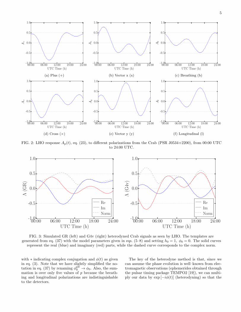
Accounting for the time dependence of the arm vectorsdue to the rotation of the Earth, eqs. (24-29) can beused to compute Ap(t) for any value of t. In fig. 2 weplot these responses for the LIGO Hanford Observatory(LHO) observing the Crab pulsar, over a sidereal day (thepattern repeats itself every day). Note that the b and l

patterns are degenerate (Ab = −√

2Al), which meansthey are indistinguishable up to an overall constant.

Although the antenna patterns are ψ–dependent, achange in this angle amounts to a rotation of A+ intoA× or of Ax into Ay, and vice–versa. If the orientationof the source is changed such that the new polarization isψ′ = ψ + ∆ψ, where ψ is the original polarization angleand ∆ψ ∈ [0, 2π], it is easy to check that the new antennapatterns can be written [23]:

A′+ = A+ cos 2∆ψ +A× sin 2∆ψ, (30)

A′× = A× cos 2∆ψ −A+ sin 2∆ψ, (31)

A′x = Ax cos ∆ψ +Ay sin ∆ψ, (32)

A′y = Ay cos ∆ψ −Ax sin ∆ψ, (33)

A′b = Ab, (34)

A′l = Al, (35)

and the tensor, vector and scalar nature of each polar-ization becomes evident from the ψ dependence.

III. METHOD

A. Data reduction

For some set of interferometric data, we would like todetect CGW signals from a given source, regardless oftheir polarization, and to reliably distinguish between thedifferent modes. Because detector response is the onlyfactor distinguishing CGW polarizations, all the relevantinformation is encoded in the amplitude modulation ofthe signal. As a result, it suffices to consider a narrowfrequency band around the GW frequency and the datacan be considerably reduced following the complex het-erodyne method developed in [24] and [20].

A signal of the form of eq. (1) can be re–written as

h(t) = Λ(t)eiφ(t) + Λ∗(t)e−iφ(t), (36)

Λ(t) =1

2

5∑p=1

apeiφp+iφ0Ap(t), (37)

5

00:00 06:00 12:00 18:00 24:00UTC Time (h)

-1.0

-0.5

0.0

0.5

1.0A

+

(a) Plus (+)

00:00 06:00 12:00 18:00 24:00UTC Time (h)

-1.0

-0.5

0.0

0.5

1.0

Ax

(b) Vector x (x)

00:00 06:00 12:00 18:00 24:00UTC Time (h)

-1.0

-0.5

0.0

0.5

1.0

Ab

(c) Breathing (b)

00:00 06:00 12:00 18:00 24:00UTC Time (h)

-1.0

-0.5

0.0

0.5

1.0

A×

(d) Cross (×)

00:00 06:00 12:00 18:00 24:00UTC Time (h)

-1.0

-0.5

0.0

0.5

1.0

Ay

(e) Vector y (y)

00:00 06:00 12:00 18:00 24:00UTC Time (h)

-1.0

-0.5

0.0

0.5

1.0

Al

(f) Longitudinal (l)

FIG. 2: LHO response Ap(t), eq. (23), to different polarizations from the Crab (PSR J0534+2200), from 00:00 UTCto 24:00 UTC.

00:00 06:00 12:00 18:00 24:00UTC Time (h)

-1.0

-0.5

0.0

0.5

1.0

Λ(G

R)

Re

Im

Norm

00:00 06:00 12:00 18:00 24:00UTC Time (h)

-1.0

-0.5

0.0

0.5

1.0

Λ(G

4v)

Re

Im

Norm

FIG. 3: Simulated GR (left) and G4v (right) heterodyned Crab signals as seen by LHO. The templates aregenerated from eq. (37) with the model parameters given in eqs. (5–8) and setting h0 = 1, φ0 = 0. The solid curves

represent the real (blue) and imaginary (red) parts, while the dashed curve corresponds to the complex norm.

with ∗ indicating complex conjugation and φ(t) as givenin eq. (3). Note that we have slightly simplified the no-tation in eq. (37) by renaming φgw0 → φ0. Also, the sum-mation is over only five values of p because the breath-ing and longitudinal polarizations are indistinguishableto the detectors.

The key of the heterodyne method is that, since wecan assume the phase evolution is well–known from elec-tromagnetic observations (ephemerides obtained throughthe pulsar timing package TEMPO2 [19]), we can multi-ply our data by exp [−iφ(t)] (heterodyning) so that the

6

signal therein becomes

h′(t) ≡ h(t)e−iφ(t) = Λ(t) + Λ∗(t)e−i2φ(t) (38)

and the frequency modulation of the first term is re-moved, while that of the second term is doubled. A se-ries of low–pass filters can then be used to remove thequickly–varying term, which enables the down–samplingof the data by averaging over minute–long time bins. Asa result, we are left with Λ(t) only and eq. (37) becomesthe template of our complex–valued signal. One periodof such GR and G4v signals coming from the Crab arepresented as seen by LHO in fig. 3.

From eq. (38) we see that, in the presence of a signal,the heterodyned and down-sampled noisy detector straindata Bk for the kth minute-long time bin (which can belabeled by GPS time of arrival) are expected to be of theform:

Bexpected(tk) =1

2

5∑p=1

ap(tk)eiφp+iφ0Ap(tk)+n(tk), (39)

where n(tk) is the heterodyned, averaged complex noisein bin k, which carries no information about the GW sig-nal. As an example, fig. 4 presents the real part of actualdata heterodyned and filtered for the Crab pulsar. Wecan clearly see already that the data are non–stationary,an issue addressed in the section III B and appendix A.

B. Search

Given data in this form, we analyze it to obtain theparameters of a signal that would best fit the data andthen incorporate the results into the frequentist analysisdescribed in section V. Regressions are performed byminimizing the χ2 of the system (same as a matched–filter). For certain template T (tk), this is:

χ2 =

N∑k=0

[T (tk)−B(tk)]2/σ2

k, (40)

where σk is the estimate standard deviation of the noisein the data at time tk. In the presence of Gaussian noise,the χ2 minimization is equivalent to a maximum likeli-hood analysis.

Any linear template T can be written as a linear com-bination of certain basis functions fi, so that T (t) =∑i

aifi(t) and each ai is found as a result of minimiz-

ing (40). For instance, T (tk) could be constructed in thefrom of eq. (37). In such model–dependent searches, theantenna patterns are the basis set, i.e. {fi} = {Ap}, andthe ai weights correspond to the ap exp (iφp) prefactors.(From here on, the tilde denotes the coefficient that isfitted for, rather than its predicted value.)

The regression returns a vector a containing the valuesof the ai’s that minimize eq. (40). These quantities are

complex–valued and encode the relative amplitude andphase of each contributing basis. From their magnitude,we define the overall recovered signal strength to be:

hrec = |a|. (41)

The significance of the fit is evaluated through the co-variance matrix C. This can be computed by taking theinverse of ATA, where A is the design matrix of the sys-tem (built from the fi set). In particular, we define thesignificance of the resulting fit (signal SNR) as

s =√a†C−1a, (42)

where † indicates Hermitian conjugation.χ2–minimizations have optimal performances when the

noise is Gaussian. However, although the central limittheorem implies that the averaged noise in (39) shouldbe normally distributed, actual data is far from this ideal(see fig. 4). In fact, the quality of the data changes overtime, as it is contingent on various instrumental factors.The time series is plagued with gaps and is highly non–stationary. This makes estimating σk non–trivial.

As done in regular CW searches [21], we address thisproblem by computing the standard deviation for thedata corresponding to each sidereal day throughout thedata run, rather than for the series as a whole. Thismethod improves the analysis because the data remainsrelatively stable over the course of a single day, but notthroughout longer periods of time (see appendix A). Fur-thermore, noisier days have less impact on the fit, becauseσk in eq. (40) will be larger. The evolution of the dailyvalue of the standard deviation for H1 data heterodynedfor the Crab pulsar is presented in fig. 5.

1. Model–dependent

In a model–dependent search, a particular physicalmodel is assumed in order to create a template basedon eq. (37). In the case of GR, if ψ and ι are known, it ispossible to construct a template with only one complex–valued free parameter h0:

TGR(t) = h01

2

[1

2(1 + cos2 ι)A+(t;ψ)+

+ cos ιA×(t;ψ)e−iπ/2], (43)

where the factor of 2 comes from the heterodyne,cf. eq. (37). Similarly for G4v:

TG4v(t) = h01

2

[sin ι e−iπ/2Ax(t;ψ) + sin ι cos ιAy(t;ψ)

],

(44)

Analogous templates could be constructed for scalar-tensor theories, or any other model. In the former case,there would be a second free parameter to represent theunknown scalar contribution.

7

FIG. 4: Real part of LIGO Science Run 5 Hanford 4km detector (H1) minute–sampled data prepared for the Crabspanning approximately two years. A signal in these data would be described by eq. (39).

FIG. 5: Daily standard deviation of S5 H1 dataheterodyned for the Crab pulsar (fig. 4).

However, as mentioned in section II, even in the caseof the best studied pulsars we know ι only in absolutevalue. This ambiguity creates the need to use two model–dependent templates like eqs. (43, 44): one correspondingto ι and one to π − ι. Note that the indeterminacy of ψis absorbed by the overall phase of h0, so it has no effecton the template. Thus, if the ambiguity in ι is accountedfor, the overall signal strength h0 and the angle φ0 can beinferred directly from the angle and phase of hrec = h0.

In most cases, ψ and ι are completely unknown. It isthen convenient to regress to each antenna pattern inde-pendently, allowing for two free parameters. This can bedone by computing the antenna patterns assuming anyarbitrary value of the polarization angle, say ψ = 0. In-deed, eqs. (30–35) guarantee that the subspace of tensor,vector or scalar antenna patterns for all ψ is spanned bya pair of corresponding tensor, vector or scalar antennapatterns assuming any particular ψ.

In the case of GR, this means we can use a template

TGR(t) = α+A+(t;ψ = 0)/2 + α×A×(t;ψ = 0)/2 (45)

with two complex weights α’s to be determined by theminimization. In the presence of a signal and in theabsence of noise, eqs. (30, 31) indicate that the valuesreturned by the fit would be a function of the actual,unknown ψ and ι:

α+ = a+(ι)eiφ0 cos 2ψ − a×(ι)eiφ0−iπ/2 sin 2ψ, (46)

α× = a×(ι)eiφ0−iπ/2 cos 2ψ + a+(ι)eiφ0 sin 2ψ, (47)

with the α(ι)’s as given in eqs. (5, 6).Again, a (semi–) model–dependent template, like

eq. (45), can be constructed for any given theory by se-lecting the corresponding antenna patterns to be used asbasis for the regression. For G4v, this would be:

TG4v(t) = αxAx(t;ψ = 0)/2 + αyAy(t;ψ = 0)/2 (48)

with two complex weights α’s to be determined by theminimization. As before, in the presence of a signal andin the absence of noise, eqs. (32, 33) indicate that thevalues returned by the fit would be a function of theactual, unknown ψ and ι:

αx = ax(ι)eiφ0−iπ/2 cosψ − ay(ι)eiφ0 sinψ, (49)

αy = ay(ι)eiφ0 cosψ + ax(ι)eiφ0−iπ/2 sinψ. (50)

In this case, we cannot directly relate our recoveredstrength to h0 and the framework does not allow to carryout parameter estimation. The proper way to do thatis using Bayesian statistics, marginalizing over the ori-entation parameters. Since we are mostly interested inquantifying our ability to detect alternative signals ratherthan estimating source parameters, we do not cover suchmethods here. However, it would be straightforward toincorporate our generalized likelihoods (as given by ourtemplates) into a full Bayesian analysis (cf. [20]).

8

2. Model–independent

In a model–independent search, the regression is per-formed using all five non–degenerate antenna patternsand the phases between the Ap’s are not constrained.Thus,

Tindep(t) =

5∑p=1

apAp(t). (51)

Because we do not consider any particular model, thereis no information about the relative strength of each po-larization; hence, the ap’s are unconstrained. Again,eqs. (30–35) enable us to compute the antenna patternsfor any value of ψ.

By calculating the necessary inner products, it can beshown that a regression to the antenna pattern basis,

{A+, A×, Ax, Ay, Ab} , (52)

is equivalent to a regression to the sidereal basis,

{1, cosωt, cos 2ωt, sinωt, sin 2ωt} , (53)

where ω = 2π/(86164 s) is the sidereal rotational fre-quency of the Earth. This is an orthogonal basis whichspans the space of the antenna patterns. In this basis,

Tindep(t) =

5∑i=1

aifi(t). (54)

with fi representing the set in (53). This is the samebasis set used in so–called 5-vector searches [25].

Because they span the same space, using either basisset yields the same results with the exact same signifi-cance, as defined in eq. (42). Furthermore, the weightsobtained as results of the fit can be converted backand forth between the two bases by means of a time–independent coordinate transformation matrix.

A model–independent search is sensitive to all polar-izations, but is prone to error due to noise when dis-tinguishing between them. It also has more degrees offreedom (compared with a pure-GR template) that canrespond to noise fluctuations, resulting in a search that isless sensitive to pure-GR signals. However, the analysiscan be followed by model–dependent searches to clarifywhich theory fits with most significance.

IV. ANALYSIS

We wish to detect any CGW signal originating in agiven pulsar, regardless of its polarization in a model–independent way. We can then determine whether themeasured polarization content agrees with theoreticalpredictions. This information can be used to obtain fre-quentist confidence levels for a potential detection and togenerate upper limits for the strength of signals of anypolarization potentially buried in the data.

In order to test the statistical properties of the noisydata filtered through our templates, we produce numer-ous instantiations of detector noise by taking actual dataprocessed as outlined in section III and re–heterodyningover a small band close to the frequency of the originalheteredoyne. Any true signal in the data stream is scram-bled in the process and what remains is a good estimateof the noise. This allows us to perform searches under re-alistic conditions with or without injections of simulatedsignals, while remaining blind to the presence of a truesignal.

By heterodyning at different frequencies, we are ableto generate a large number of instantiations of the data.Because our S5 datasets span roughly 1.9 years and aresampled once per minute, our bandwidth is 8.3×10−3 Hzwith a lowest resolvable frequency of 1.7×10−8 Hz. Thismeans we could theoretically re–heterodyne our data ata maximum of 8.3×10−3/1.7×10−8 ≈ 4.9×105 indepen-dent frequencies. In our study, we picked 104 frequenciesin the 10−7−10−3 Hz range, avoiding the expected signalfrequency of ∼ 10−5 Hz (period of a sidereal day) and itsmultiples.

We quantify the results of a particular search by look-ing at the obtained recovered signal strength, eq. (41),and significance, eq. (42). As expected, these two pa-rameters are strongly correlated (fig. 6). However, thesignificance is, in the presence of Gaussian noise, a directindicator of goodness–of–fit and can be used to compareresults from templates with different numbers of degreesof freedom.

By performing searches on multiple instantiations ofnoise–only data, we construct cumulative distributionfunction (CDF) probability plots showing the distribu-tion of recovered signal strength, eq. (41), and signifi-cance, eq. (42), corresponding to a given template. Suchplots give the probability that the outcome of the re-gression is consistent with noise (i.e. provide p–values).As shown in fig. 7, an instantiation that contains a loudinjected signal becomes manifest in this plot as an out-lier. This sort of plot can also be used when searchingfor an actual signal in the data—namely, when lookingat the original, non–reheterodyned series. In that case,the 1 − CDF curve can be extrapolated or interpolatedto find the p–value corresponding to the significance withwhich the injection was recovered.

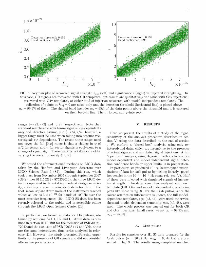
After injecting and retrieving increasingly loud signalswith a given polarization content in different backgroundinstantiations, we produce plots of recovered strengthvs. injected strength (hrec vs. hinj) and significance vs. in-jected strength (s vs. hinj). Recall that injections are ofthe form of eqs. (43, 44). Examples of such plots are pre-sented in fig. 8. These plots, and corresponding fits, canbe used to assess the sensitivity of a template to certaintype of signal, define thresholds for detection and pro-duce confidence bands for recovered parameters. (In thefrequentist literature, these plots are sometimes referredto as Neyman constructions [26].)

We define a horizontal detection threshold line above

9

FIG. 6: Significance, eq. (42), vs. recovered strength, eq. (41), for searches over 5000 noise–only H1 S5 Crabinstantiations using model–dependent eq. (43) (left), semi–dependent eq. (45) (center), and independent eq. (54)(right) templates. The model–dependent case assumes fully known ι and ψ. Note that the number of degrees offreedom in the regression is manifested in the spread, which is due to noise: templates with a single degree of

freedom are less susceptible to noise and the spread is minimal. The two plots on the left were generated using a GRtemplate, but similar results are obtained for G4v.

FIG. 7: Example plot of p = 1− CDF vs. the recoverysignificance for a particular template. A loud injection

in noise is manifested as an outlier (star) over thenoise–only background (red). Note that the injection is

plotted arbitrarily at p = 10−1.

an arbitrary fraction αn (e.g., αn = 99.9%) of noise–onlypoints (i.e. points with hinj = 0, but hrec 6= 0), so thatdata points above this line can be considered detectedwith a p–value of p = 1−αn (e.g., p = 0.1%). For a par-ticular template, this fractional threshold can be directlytranslated into a significance value sαn

(e.g., s99.9% =2.5). The sensitivity of the template is related to thenumber of injections recovered with a significance higherthan sαn

. Therefore, for a given αn, a lower sαnmeans

higher sensitivity to true signals.

For the results of each template, the fractional thresh-old αn can also be associated to a strain value. We definethis to be the loudness of the minimum injection detected

above this threshold with some arbitrary upper–limit con-fidence αup. This value can be determined from the svs. hinj plot by placing a line parallel to the best fit butto the right of a fraction αup of all data points satisfying0 < hinj. The intersection of this line with the αn lineoccurs at hinj = h

αup

min, which is the strain value abovewhich we can have αup confidence that a signal will bedetected (i.e. recovered with significance s > sαn

).We refer to h

αup

min as the expected sensitivity or straindetection threshold at αn. This value allows not onlyfor the definition of upper limits for the presence of sig-nals, but also the comparison of different model depen-dent and independent templates. See fig. 9b for a jux-taposition of the results of matching and non–matchingmodel–dependent templates for the case of the Crab pul-sar.

The efficiency of a template is also quantified by theslope of the hrec vs. hinj best–fit line, which should beclose to 1 for a template that matches the signal. Weperform this fit by taking into account only points abovethe αn line and forcing the y–intersect to be null. The de-viations from this fit are used to produce confidence inter-vals for the recovered strength. This is done by defining aband centered on the best–fit line and enclosing an arbi-trary fraction αb (e.g., αb = 95%) of the data points, cor-responding to the confidence band placed around best–fitline. The intersection between this band and a horizon-tal line at some value of hrec yields a confidence intervalfor the true strength with αb confidence. Note that de-viations above and below the best–fit line are taken in-dependently to obtain asymmetric confidence intervals.The same analysis can be done on the s vs. hinj plots,taking into account proper scaling of the best–fit slope.

In general, when performing injections we pick param-eters with a uniform distribution over the uncertaintyranges of location and orientation values obtained fromthe ATNF Pulsar Catalog [27]. When there is no ori-entation information, we must draw ψ and ι from the

10

FIG. 8: Neyman plot of recovered signal strength hrec (left) and significance s (right) vs. injected strength hinj. Inthis case, GR signals are recovered with GR templates, but results are qualitatively the same with G4v injections

recovered with G4v templates, or either kind of injection recovered with model–independent templates. Thecollection of points at hinj = 0 are noise–only and the detection threshold (horizontal line) is placed above

αn = 99.9% of them. The shaded band includes αb = 95% of the data points above the threshold and it is centeredon their best–fit line. The fit forced null y–intersect.

ranges [−π/2, π/2] and [0, 2π] respectively. Note thatstandard searches consider tensor signals (2ψ–dependent)only and therefore assume ψ ∈ [−π/4, π/4]; however, abigger range must be used when taking into account vec-tor signals (ψ–dependent). The reason these ranges neednot cover the full [0, π] range is that a change in ψ ofπ/2 for tensor and π for vector signals is equivalent to achange of signal sign. Therefore, this is taken care of byvarying the overall phase φ0 ∈ [0, π].

We tested the aforementioned methods on LIGO datataken by the Hanford and Livingston detectors overLIGO Science Run 5 (S5). During this run, whichtook place from November 2005 through September 2007(GPS times 815155213 - 875232014), the three LIGO de-tectors operated in data–taking mode at design sensitiv-ity, collecting a year of coincident detector data. Theroot–mean–square strain noise of the instrument reachedvalues as low as 3 × 10−22 for bands of 100 Hz over themost sensitive frequencies [28]. LIGO S5 data has beenrecently released to the public and is accessible onlinethrough the LIGO Open Science Center [29].

In particular, we looked at data for 115 pulsars, ob-tained by reducing S5 H1, H2 and L1 strain data as out-lined in section III B. But for the inclusion of PSR J0024-72040 and the exclusion of PSR J2033+17 and Vela, theseare the same heterodyned time series analyzed in refer-ence [21]. However, that study presented Bayesian upperlimits to the presence of GR signals and did not consideralternative polarizations.

V. RESULTS

Here we present the results of a study of the signalsensitivity of the analysis procedure described in sec-tion V, using the data described at the end of section. We perform a “closed box” analysis, using only re–heterodyned data, which are insensitive to the presenceof actual signals, and simulated signal injections. A full“open box” analysis, using Bayesian methods to producemodel–dependent and model–independent signal detec-tion confidence bands or upper limits, is in preparation.

In particular, we produced 104 re–heterodyned instan-tiations of data for each pulsar by picking linearly spacedfrequencies in the 10−7−10−3 Hz range (cf. sec. V). Halfof those were injected with simulated signals of increas-ing strength. The data were then analyzed with eachtemplate (GR, G4v and model–independent), producingplots like those in fig. 8. For the Crab pulsar, since thesource orientation information is known, the full model–dependent templates, eqs. (43, 44), were used; otherwise,the semi–model–dependent templates, eqs. (45, 48), wereused. The whole process was carried out for both GRand G4v injections. In all cases, we set αn = 99.9% andαup = 95.0%.

A. Crab pulsar

Results for searches over H1 S5 data prepared for theCrab pulsar (ν = 30.22 Hz, νGW = 60.44 Hz) are pre-sented in fig. 9. The results using templates matched

11

(a) GR injections recovered with GR template (green),eq. (45), and model independent (blue), eq. (54).

(b) GR injections recovered with GR template (green),eq. (45), and G4v template (red), eq. (48).

(c) G4v injections recovered with G4v template (red),eq. (48), and model independent (blue), eq. (54).

(d) G4v injections recovered with G4v template (red), eq. (48),and GR template (green), eq. (45).

FIG. 9: GR (top) and G4v (bottom) injection results of search over LIGO S5 H1 data heterodyned for the Crabpulsar. Plots show significance, eq. (42), vs. injected strength. Color corresponds to the template used for recovery:GR, green; G4v, red; model–independent, blue. This particular search was performed using 104 instantiations, halfof which contained injections using the values of ι and ψ given in table I. The model–dependent templates assumed

the same same ι as the injections. Horizontal lines correspond to a detection threshold αn = 99.9%.

to the injections are compared to those of the model–independent (left) and non–matching templates (right).The expected sensitivities, as defined in section V, foreach injection template and search model are providedin table III. Recall that the Crab is a special case, sinceits orientation in the sky is well–known, which enablesus to use full model–dependent templates, eqs. (43, 44).However, searches for actual signals would still have tomake use to two templates for each theoretical model be-

cause of the ambiguity in ι described in section II B. Inorder to avoid doing this, a semi–model–dependent ormodel–independent search could be carried out instead.

A number of interesting observations can be drawnfrom fig. 9 and table III. As inferred from the valuesof hmin, the model–independent template is roughly 25%less sensitive than the matching one, regardless of thetheory assumed when making injections. This is under-stood by the presence of four extra degrees of freedom in

12

102 103

GW Frequency [Hz]

1023

1024

1025

1026S

lop

e(s

vs.h

inj)

GR

G4v

Indep

(a) GR slope

102 103

GW Frequency [Hz]

1023

1024

1025

1026

Slo

pe

(svs

.h

inj)

GR

G4v

Indep

(b) G4v slope

102 103

GW Frequency [Hz]

1

2

3

4

5

6

7

8

9

s

GR

G4v

Indep

(c) Detection threshold

FIG. 10: Slope of the s vs. hinj best–fit–line (left and center) and significance detection threshold at αn = 99.9%(right) vs. GW frequency and for GR and G4v injections on S5 H1 data for 115 pulsars. Color corresponds to search

template: GR, green; G4v, red; and model–independent, blue. Note that for both kinds of injections, themodel–independent points overlap the matching template.

TABLE III: Summary of expected sensitivity for theCrab pulsar S5 H1 searches (αn = 99.9%, αup = 95.0%).

Rows correspond to injection type and columns tosearch template. The rotational frequency of the Crab

is ν = 30.22 Hz and, therefore, νGW = 60.44 Hz.

GR G4v Independent

GR 3.41 × 10−25 7.49 × 10−25 4.20 × 10−25

G4v 8.90 × 10−25 3.30 × 10−25 4.15 × 10−25

the model–independent template, compared to the singletunable coefficient in the full model–dependent one. If in-stead the semi–model–dependent template with two de-grees of freedom is used, the improvement with respect tothe model–independent search goes down to 15%. In anycase, the accuracy of matching and model–independentsearches, given by the width of the confidence bands an,are almost identical.

Model dependent templates are significantly less sen-sitive to non–matching signals. Table III indicates thatmodel–dependent templates are 120-170% less sensitiveto non–matching signals than their matching counter-part. A consequence of this is the existence of a rangeof signals which would be detected by templates of onetheory, but not the other (see figs. 9b & 9d). This is par-ticularly interesting, given that previous LIGO searchesassume GR to be valid and use a template equivalent toeq. (43). Therefore, our results suggest it is possible thatthose searches might have missed fully–non–GR signalsburied in the data (see section VI for further discussion).

TABLE IV: Best expected sensitivities for S5 H1searches (αn = 99.9%, αup = 95.0%). Rows correspondto injection type and columns to pulsar name (PSR),rotation frequency (ν) and strain detection threshold

for matching dependent (hdep) and independent (hindep)templates.

PSR ν (Hz) hdep hindep

GR J1603-7202 67.38 4.77 × 10−26 5.53 × 10−26

G4v J1748-2446A 86.48 4.96 × 10−26 5.81 × 10−26

B. All pulsars

The Crab pulsar is only one of the 115 sources we an-alyzed. The results, presented in figs. 10a & 10b gener-ally confirm the observations anticipated from the Crab.While model–independent searches are of the same ac-curacy as matching semi–model–dependent ones, theirstrain detection threshold is louder due to the extradegrees of freedom (fig. 10c). Consequently, model–independent templates demand a higher significance tobe able to distinguish a signal from noise. The detectionthresholds for GR and G4v templates are of the samemagnitude, since both have the same number of degreesof freedom. Among all the 115 pulsars, the sources withbest expected sensitivities to GR and G4v signals werePSR J1603-7202 and PSR J1748-2446A respectively (seetable IV).

The key results of our study are summarized in fig. 11for H1 and fig. 12 for L1. These plots present the ex-pected sensitivity (strain detection threshold at αn =99.9% with αup = 95.0% confidence) vs. GW frequency(νGW = 2ν). The outliers seen in figs. 10-12 correspondto pulsars whose value of νGW are very close to instru-mental noise spectral lines associated with violin reso-

13

102 103

Gravitational-wave Frequency (Hz)

10−27

10−26

10−25

10−24

10−23

Det

ecti

onth

resh

old

(str

ain

)

Number of pulsars: 115

Detection threshold: 0.999

Detection confidence: 0.95

Expected: H1 S5

Indep template

GR template

(a) GR injections

102 103

Gravitational-wave Frequency (Hz)

10−27

10−26

10−25

10−24

10−23

Det

ecti

onth

resh

old

(str

ain

)

Number of pulsars: 115

Detection threshold: 0.999

Detection confidence: 0.95

Expected: H1 S5

Indep template

G4v template

(b) G4v injections

FIG. 11: S5 H1 expected sensitivity (strain detection threshold at αn = 99.9% with αup = 95.0% confidence)vs. GW frequency for 115 pulsars. Color corresponds to search template: GR, green; G4v, red; and

model–independent, blue. The gray line is the anticipated sensitivity of a standard Bayesian search, eq. (55).

14

102 103

Gravitational-wave Frequency (Hz)

10−27

10−26

10−25

10−24

10−23

Det

ecti

onth

resh

old

(str

ain

)

Number of pulsars: 115

Detection threshold: 0.999

Detection confidence: 0.95

Expected: L1 S5

Indep template

GR template

(a) GR injections

102 103

Gravitational-wave Frequency (Hz)

10−27

10−26

10−25

10−24

10−23

Det

ecti

onth

resh

old

(str

ain

)

Number of pulsars: 115

Detection threshold: 0.999

Detection confidence: 0.95

Expected: L1 S5

Indep template

G4v template

(b) G4v injections

FIG. 12: S5 L1 expected sensitivity (strain detection threshold at αn = 99.9% with αup = 95.0% confidence) vs. GWfrequency for 115 pulsars. Color corresponds to search template: GR, green; G4v, red; and model–independent,

blue. The gray line is the anticipated sensitivity of a standard Bayesian search, eq. (55).

15

TABLE V: Average sensitivity ratios 〈ρ〉, eq. (56), forS5 H1 (first value) and S5 L1 (second value) searches.

Rows correspond to injection type and columns tosearch template.

GR G4v Independent

GR 16.11 14.65 58.53 51.89 18.83 17.15

G4v 61.21 55.06 18.42 16.76 21.24 19.32

TABLE VI: Crab sensitivity ratio ρ, eq. (56) evaluatedat the Crab’s GW frequency, for S5 H1 (first value) and

S5 L1 (second value) searches. Rows correspond toinjection type and columns to search template.

GR G4v Independent

GR 20.75 10.40 45.52 27.15 25.54 11.94

G4v 54.06 20.30 20.07 9.96 25.21 11.52

nances of the detectors test mass pendulum suspensions.For the matching or model–independent templates, the

resulting data points trace the noise curve of the in-strument; however, due to the long integration time, weare able to detect signals below LIGO’s standard strainnoise. The gray curve shown in figs. 11, 12 representsthe expected sensitivity of a regular Bayesian GR search(e.g., [21]). This is proportional to the amplitude spec-tral density of the detector and inversely proportional tothe square–root of the observation time. The particu-lar empirical relationship used to generate the curve infigs. 11 & 12 is:

〈hmin〉 = 10.8√Sn(f)/T , (55)

with Sn(f) the noise power spectral density and T the to-tal observation time (527 days for S5 H1 and 405 days forS5 L1) [20]. This formula enables the comparison of themethods presented here with the expected performanceof standard Bayesian searches.

By the same token, we can define a figure of merit ρfor our searches by the ratio:

ρ (νGW) = hmin/√Sn(νGW)/T . (56)

The average of this value over all pulsars, 〈ρ〉, can besemi–quantitatively compared to the 10.8 prefactor ineq. (55). The equivalence is not direct because, besidesthe intrinsic differences between Bayesian and frequen-tist approaches, eq. (55) was obtained by averaging theresults of 4000 simulated searches [20], while we includejust the 115 pulsars at hand. The values of 〈ρ〉 for our S5H1 & L1 analyses are presented in table V and fig. 13.The specific values for the Crab pulsar are shown in tableVI. A smaller ρ indicates better performance.

As mentioned above, the remarks made about theCrab pulsar hold for most other sources, except that de-

0 20 40 60 80 100 120 140 160 180ρ

0

10

20

30

40

50

Cou

nt

GR

G4v

Indep

(a) H1 GR

0 20 40 60 80 100 120 140 160ρ

0

5

10

15

20

25

30

35

40

Cou

nt

GR

G4v

Indep

(b) H1 G4v

0 20 40 60 80 100 120 140 160 180ρ

0

5

10

15

20

25

30

35

40

Cou

nt

GR

G4v

Indep

(c) L1 GR

0 20 40 60 80 100 120 140 160ρ

0

5

10

15

20

25

30

35

40

Cou

nt

GR

G4v

Indep

(d) L1 G4v

FIG. 13: Histograms of the figure of merit ρ, eq. (56),for our searches over S5 H1 (top) and L1 (bottom) data

sets with GR (left) and G4v (right) injections,corresponding to 115 pulsars. Color corresponds to

search template: GR, green; G4v, red; andmodel–independent, blue.

tectability is slightly lower because orientation parame-ters are unknown. In all cases, the matching templateis the best at recovering signals, followed closely by themodel–independent one. Searches that assume the incor-rect model are substantially less efficient and their hmin

vs. νGM curves do not follow the instrumental noise line.This is reflected, for instance, by the figures of merit pre-sented in table V.

VI. CONCLUSIONS

We have developed novel model–independent methodsto search for CGW signals coming from targeted sourcesin LIGO–like interferometric data. These searches areable to detect signals of any polarization content withhigh significance.

In order to test our methods in the presence of realisticnoise conditions, we implemented a procedure to producethousands of noise–only instantiations from actual data.We then proceeded by injecting and retrieving increas-ingly loud signals of different polarization content.

We studied 115 pulsars using S5 data from the LIGOHanford and Livingston detectors. Although the meth-ods are general, we restricted our study to two theoriesthat predict starkly different GW polarization contents(GR and G4v).

Our results indicate that assuming the wrong the-oretical model greatly reduces the sensitivity of a

16

search to signals buried in the data. Yet, our model–independent searches are almost as effective as themodel–dependent templates that match the kind of sig-nal injected (i.e. when the models used for injectionand search are the same). This means that our model–independent templates can be used to find signals of anypolarizations without additional computational require-ments.

We are able to reach sensitivities comparable to previ-ous studies, although slightly worse than those presentedin [21]. This is probably due to our making use of a sin-gle detector and to differences between frequentist andBayesian approaches.

We have shown that, for some combinations of detec-tors, sources, and signal strengths, G4v signals are in-visible to GR templates and vice–versa. Therefore, it ispossible that, if GWs are composed uniquely of vectormodes, previous LIGO searches, which assume GR, mayhave missed their signals.

It is clear that the next step in this study consists ofincorporating our model–independent templates into theBayeasian machinery used in standard LIGO ScientificCollaboration searches. This will allow us to properlymarginalize over all nuisance parameters and to producemulti-detector model–dependent and model–independentsignal detection confidence bands or upper limits. Wewill also employ methods to constrain other theories(e.g., scalar–tensor) in the event of a model-independentdetection.

ACKNOWLEDGMENTS

The authors would like to thank Holger Pletsch forhelpful discussions. M. Pitkin is funded by the STFCthrough grant number ST/L000946/1. LIGO was con-structed by the California Institute of Technology andMassachusetts Institute of Technology with funding fromthe National Science Foundation and operates under co-operative agreement PHY-0757058. This paper carriesLIGO Document Number LIGO-P1400169.

Appendix A: Statistical properties of LIGO data

The χ2 minimization is equivalent to a maximum like-lihood procedure only in the presence of Gaussian noise.When this requirement is not satisfied, the regression isstill valid, but the χ2 values resulting from the fit willbe distributed in a non–trivial way, rather than the χ2

distribution expected in the case of Gaussian noise. Fur-thermore, the relationship between the covariance matrix

of the system and the standard uncertainties of the recov-ered coefficients becomes unclear. Therefore, it is impor-tant to statistically characterize the data and understandthe limitations of our assumption of Gaussianity.

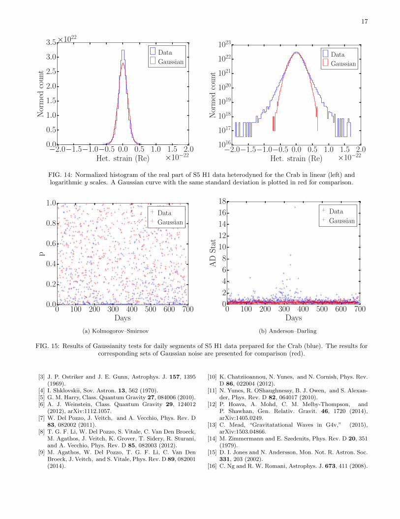
When taken as a whole, LIGO detector noise does notconform to a stationary Gaussian distribution. This canbe visually confirmed by means of a histogram, as shownin fig. 14 for the case of S5 H1 data prepared for theCrab. The divergence from Gaussianity is evident fromthe long tails, seen most clearly in the log–y version of theplot. As expected, the data fail more rigorous standardGaussianity tests, such as the Kolmogorov–Smirnov (KS)or the Anderson–Darling (AD) tests.

However, it is possible to split up the data into day–long (or shorter) segments, as was described in sectionIII B, so as to study the Gaussianity of the data on aday–to–day basis. The results of the KS and AD testsfor each day–segment, together with those for referenceGaussian noise series, are presented in figs. 15a and 15brespectively. The KS test returns the p–value for a nullhypothesis that assumes the data is normally distributed;therefore, a lower p–value implies a higher probabilitythat the data are not Gaussian [30]. The AS test re-turns a figure of merit which is indirectly proportional tothe significance with which the hypothesis of Gaussianitycan be rejected; therefore a higher AS statistic implies ahigher probability that the data are not Gaussian [31].

It can be seen from the results of these tests that thestatistical properties of the segments vary considerablyfrom day to day. This could have been guessed from thenon-stationarity of the data in fig. 4, the daily variation ofthe standard deviation (fig. 5) and other irregularities ofthe data. Nonetheless, most of the segments seem to passthe Gaussianity tests, with some remarkable exceptionsaround the days 250–400 of the run. This correspondsto the spiking observed in the heterodyned data (GPStimes 8.4× 108 − 8.5× 108 in fig. 4).

In order to confirm that our assumption of Gaussian-ity is not too far from reality, we repeated our analysis(see section V) on sets of synthetic Gaussian noise. Inorder to do this, for each pulsar we generated streamsof complex–valued data randomly selected from a nor-mal distribution with the same standard deviation as thecorresponding original LIGO data set. These series re-placed the instantiations of re–heterodyned data, but thesearch process was otherwise unchanged. The results ofthis comparison for S5 H1 are shown in figs. 16, where wejuxtaposed expected sensitivities obtained using Gaus-sian noise and actual LIGO noise (cf. section V). Theseplots confirm that, indeed, we obtain qualitatively thesame results with Gaussian noise as with actual LIGOdata.

[1] C. M. Will, Living Rev. Relativ. 17 (2014), 10.12942/lrr-2014-4.

[2] S. G. Turyshev, Annu. Rev. Nucl. Part. Sci. 58, 30(2008), arXiv:0806.1731.

17

−2.0−1.5−1.0−0.5 0.0 0.5 1.0 1.5 2.0Het. strain (Re) ×10−22

0.0

0.5

1.0

1.5

2.0

2.5

3.0

3.5N

orm

edco

unt

×1022

Data

Gaussian

−2.0−1.5−1.0−0.5 0.0 0.5 1.0 1.5 2.0Het. strain (Re) ×10−22

1016

1017

1018

1019

1020

1021

1022

1023

Nor

med

cou

nt

Data

Gaussian

FIG. 14: Normalized histogram of the real part of S5 H1 data heterodyned for the Crab in linear (left) andlogarithmic y scales. A Gaussian curve with the same standard deviation is plotted in red for comparison.

0 100 200 300 400 500 600 700Days

0.0

0.2

0.4

0.6

0.8

1.0

p

Data

Gaussian

(a) Kolmogorov–Smirnov

0 100 200 300 400 500 600 700Days

0

2

4

6

8

10

12

14

16

18

AD

Sta

tData

Gaussian

(b) Anderson–Darling

FIG. 15: Results of Gaussianity tests for daily segments of S5 H1 data prepared for the Crab (blue). The results forcorresponding sets of Gaussian noise are presented for comparison (red).

[3] J. P. Ostriker and J. E. Gunn, Astrophys. J. 157, 1395(1969).

[4] I. Shklovskii, Sov. Astron. 13, 562 (1970).[5] G. M. Harry, Class. Quantum Gravity 27, 084006 (2010).[6] A. J. Weinstein, Class. Quantum Gravity 29, 124012

(2012), arXiv:1112.1057.[7] W. Del Pozzo, J. Veitch, and A. Vecchio, Phys. Rev. D

83, 082002 (2011).[8] T. G. F. Li, W. Del Pozzo, S. Vitale, C. Van Den Broeck,

M. Agathos, J. Veitch, K. Grover, T. Sidery, R. Sturani,and A. Vecchio, Phys. Rev. D 85, 082003 (2012).

[9] M. Agathos, W. Del Pozzo, T. G. F. Li, C. Van DenBroeck, J. Veitch, and S. Vitale, Phys. Rev. D 89, 082001(2014).

[10] K. Chatziioannou, N. Yunes, and N. Cornish, Phys. Rev.D 86, 022004 (2012).

[11] N. Yunes, R. OShaughnessy, B. J. Owen, and S. Alexan-der, Phys. Rev. D 82, 064017 (2010).

[12] P. Hoava, A. Mohd, C. M. Melby-Thompson, andP. Shawhan, Gen. Relativ. Gravit. 46, 1720 (2014),arXiv:1405.0249.

[13] C. Mead, “Gravitatational Waves in G4v,” (2015),arXiv:1503.04866.

[14] M. Zimmermann and E. Szedenits, Phys. Rev. D 20, 351(1979).

[15] D. I. Jones and N. Andersson, Mon. Not. R. Astron. Soc.331, 203 (2002).

[16] C. Ng and R. W. Romani, Astrophys. J. 673, 411 (2008).

18

102 103

Gravitational-wave Frequency (Hz)

10−27

10−26

10−25

10−24

10−23

Str

ain

Sen

siti

vity

Expected: H1 S5

GR template (Gaussian noise)

GR template

(a) GR injections on Gaussian noise

102 103

Gravitational-wave Frequency (Hz)

10−27

10−26

10−25

10−24

10−23

Str

ain

Sen

siti

vity

Expected: H1 S5

G4v template (Gaussian noise)

G4v template

(b) G4v injections on Gaussian noise

FIG. 16: Expected sensitivity (αn = 99.9%, αup = 95.0%) vs. GW frequency. Comparison between fabricatedGaussian noise and actual LIGO noise. Searches were made with semi–model–dependent templates, eqs. (45, 48).The colored stars correspond to actual LIGO H1 noise (cf. fig. 11), while the black dots correspond to fabricated

Gaussian noise.

19

[17] W. Althouse, L. Jones, and A. Lazzarini, Determinationof Global and Local Coordinate Axes for the LIGO Sites(LIGO-T980044), Tech. Rep. (LIGO, 2001).

[18] B. Allen, Gravitational Wave Detector Sites, Tech.Rep. (University of Wisconsin–Milwaukee, 1996)arXiv:9607075 [gr-qc].

[19] R. T. Edwards, G. B. Hobbs, and R. N. Manch-ester, Mon. Not. R. Astron. Soc. 372, 1549 (2006),arXiv:0607664 [astro-ph].

[20] R. Dupuis and G. Woan, Phys. Rev. D 72, 102002 (2005),arXiv:0508096 [gr-qc].

[21] The LIGO Scientific Collaboration and The VirgoCollaboration, Astrophys. J. 713, 671 (2010),arXiv:0909.3583.

[22] A. Nishizawa, A. Taruya, K. Hayama, S. Kawamura, andM.-a. Sakagami, Phys. Rev. D 79, 082002 (2009).

[23] A. Baut, Phys. Rev. D 85, 043005 (2012).[24] T. M. Niebauer, A. Rudiger, R. Schilling, L. Schnupp,

W. Winkler, and K. Danzmann, Phys. Rev. D 47, 3106

(1993).[25] P. Astone, S. DAntonio, S. Frasca, and C. Palomba,

Class. Quantum Gravity 27, 194016 (2010).[26] A. Olive et al. and Particle Data Group, Chinese Phys.

C 38, 090001 (2014).[27] R. N. Manchester, G. B. Hobbs, A. Teoh, and M. Hobbs,

Astron. J. 129, 1993 (2005), arXiv:0412641 [astro-ph].[28] The LIGO Scientific Collaboration, Reports Prog. Phys.

72, 076901 (2009), arXiv:0711.3041.[29] M. Vallisneri, J. Kanner, R. Williams, A. Weinstein, and

B. Stephens, in Proc. LISA Symp. X (IOP Publishing,Gainesville, Florida, 2014) arXiv:1410.4839.

[30] I. M. Chakravarty, J. D. Roy, and R. G. Laha, Handbookof methods of applied statistics Volume I (John Wileyand Sons, New York, 1967) pp. 392–394.

[31] T. W. Anderson and D. A. Darling, Ann. Math. Stat. 23,193 (1952).