Isentropic Analysis Much of this presentation is due to Jim Moore, SLU

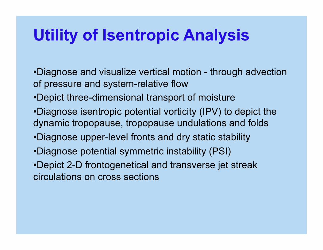
Utility of Isentropic Analysis

• Diagnose and visualize vertical motion - through advection of pressure and system-relative flow • Depict three-dimensional transport of moisture • Diagnose isentropic potential vorticity (IPV) to depict the dynamic tropopause, tropopause undulations and folds • Diagnose upper-level fronts and dry static stability • Diagnose potential symmetric instability (PSI) • Depict 2-D frontogenetical and transverse jet streak circulations on cross sections

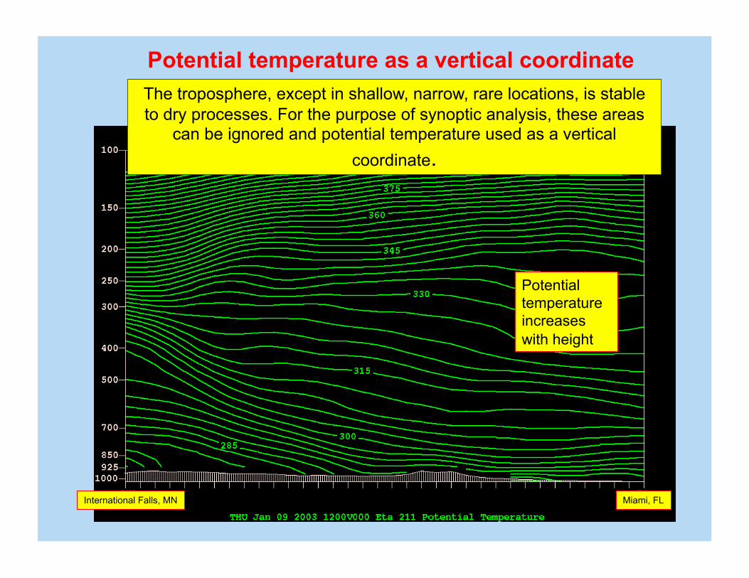
The troposphere, except in shallow, narrow, rare locations, is stable to dry processes. For the purpose of synoptic analysis, these areas

can be ignored and potential temperature used as a vertical coordinate.

Potential temperature increases with height

International Falls, MN Miami, FL

Potential temperature as a vertical coordinate

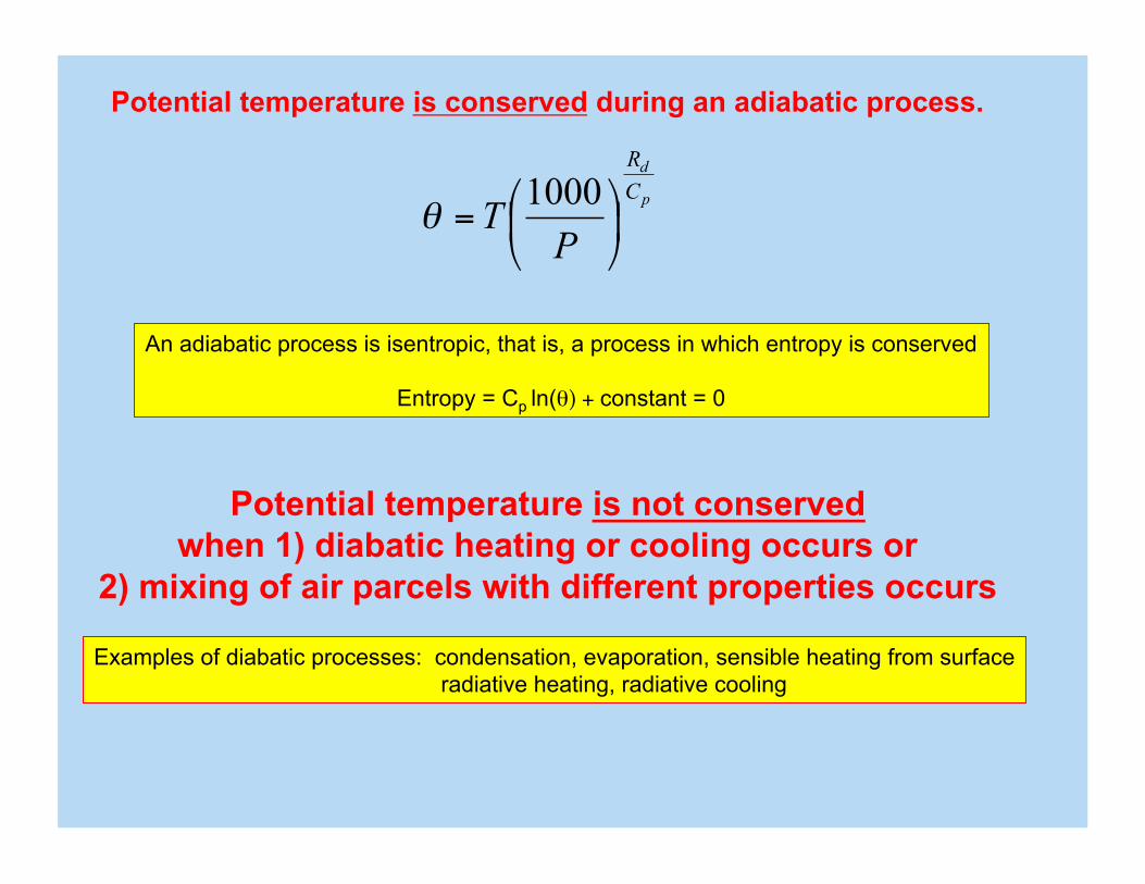
An adiabatic process is isentropic, that is, a process in which entropy is conserved

Entropy = Cp ln(θ) + constant = 0

p

dCR

PT ⎟

⎠

⎞⎜⎝

⎛=1000

θ

Potential temperature is conserved during an adiabatic process.

Potential temperature is not conserved when 1) diabatic heating or cooling occurs or

2) mixing of air parcels with different properties occurs

Examples of diabatic processes: condensation, evaporation, sensible heating from surface radiative heating, radiative cooling

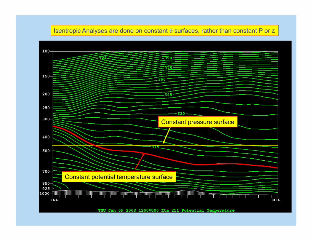
Isentropic Analyses are done on constant θ surfaces, rather than constant P or z

Constant pressure surface

Constant potential temperature surface

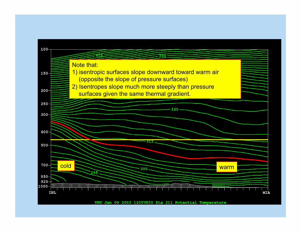
Note that: 1) isentropic surfaces slope downward toward warm air (opposite the slope of pressure surfaces) 2) Isentropes slope much more steeply than pressure surfaces given the same thermal gradient.

cold warm

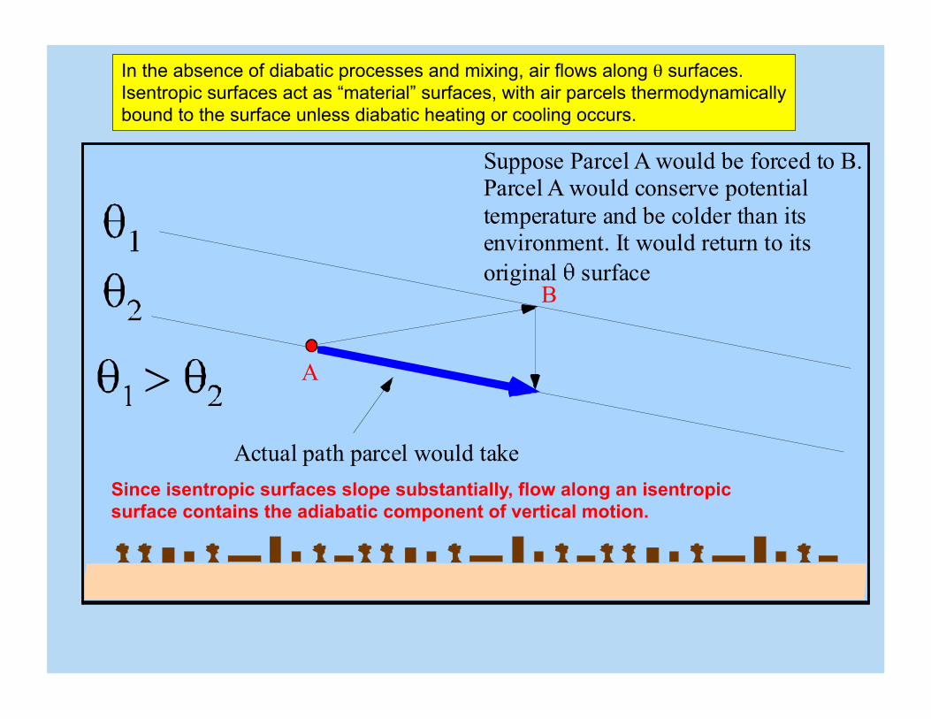
Suppose Parcel A would be forced to B.Parcel A would conserve potentialtemperature and be colder than itsenvironment. It would return to itsoriginal surface

A

B

Actual path parcel would take

In the absence of diabatic processes and mixing, air flows along θ surfaces. Isentropic surfaces act as “material” surfaces, with air parcels thermodynamically bound to the surface unless diabatic heating or cooling occurs.

Since isentropic surfaces slope substantially, flow along an isentropic surface contains the adiabatic component of vertical motion.

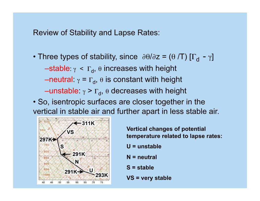
Review of Stability and Lapse Rates:

•  Three types of stability, since ∂θ/∂z = (θ /T) [Γd - γ] – stable: γ < Γd, θ increases with height – neutral: γ = Γd, θ is constant with height – unstable: γ > Γd, θ decreases with height

•  So, isentropic surfaces are closer together in the vertical in stable air and further apart in less stable air.

Vertical changes of potential temperature related to lapse rates:

U = unstable

N = neutral

S = stable

VS = very stable

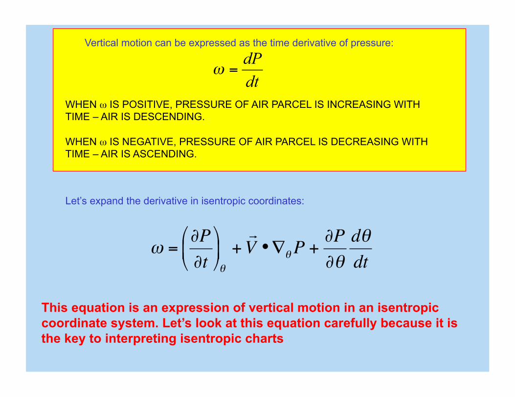
Vertical motion can be expressed as the time derivative of pressure:

dtdP

=ω

Let’s expand the derivative in isentropic coordinates:

€

ω =∂P∂t

⎛

⎝ ⎜

⎞

⎠ ⎟ θ

+

V •∇θ P +∂P∂θ

dθdt

This equation is an expression of vertical motion in an isentropic coordinate system. Let’s look at this equation carefully because it is the key to interpreting isentropic charts

WHEN ω IS POSITIVE, PRESSURE OF AIR PARCEL IS INCREASING WITH TIME – AIR IS DESCENDING.

WHEN ω IS NEGATIVE, PRESSURE OF AIR PARCEL IS DECREASING WITH TIME – AIR IS ASCENDING.

€

ω =∂P∂t

⎛

⎝ ⎜

⎞

⎠ ⎟ θ

+ V •∇θ P +

∂P∂θ

dθdt

Let’s start with the second term:

€

V •∇θ P = u ∂P

∂x⎛

⎝ ⎜

⎞

⎠ ⎟ θ

+ v ∂P∂y⎛

⎝ ⎜

⎞

⎠ ⎟ θ

θ

⎟⎠

⎞⎜⎝

⎛∂∂xP

y

x

N

E

550 560 570 580 590 600

u

y

x

N

E

550

560

570

580

590

600

v

θ⎟⎟⎠

⎞⎜⎜⎝

⎛

∂∂yP

Pressure advection: When the wind is blowing across the isobars on an isentropic chart toward higher pressure, air is descending (ω is positive) When the wind is blowing across the isobars on an isentropic chart toward lower pressure, air is ascending (ω is negative)

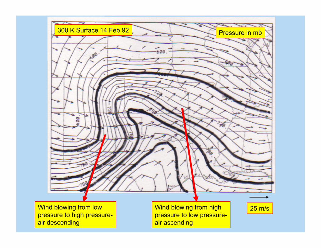
300 K Surface 14 Feb 92 Pressure in mb

25 m/s Wind blowing from low pressure to high pressure- air descending

Wind blowing from high pressure to low pressure- air ascending

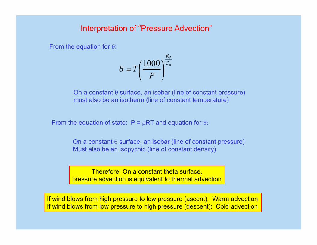
Interpretation of “Pressure Advection”

From the equation for θ:

p

dCR

PT ⎟

⎠

⎞⎜⎝

⎛=1000

θ

On a constant θ surface, an isobar (line of constant pressure) must also be an isotherm (line of constant temperature)

From the equation of state: P = ρRT and equation for θ:

On a constant θ surface, an isobar (line of constant pressure) Must also be an isopycnic (line of constant density)

Therefore: On a constant theta surface, pressure advection is equivalent to thermal advection

If wind blows from high pressure to low pressure (ascent): Warm advection If wind blows from low pressure to high pressure (descent): Cold advection

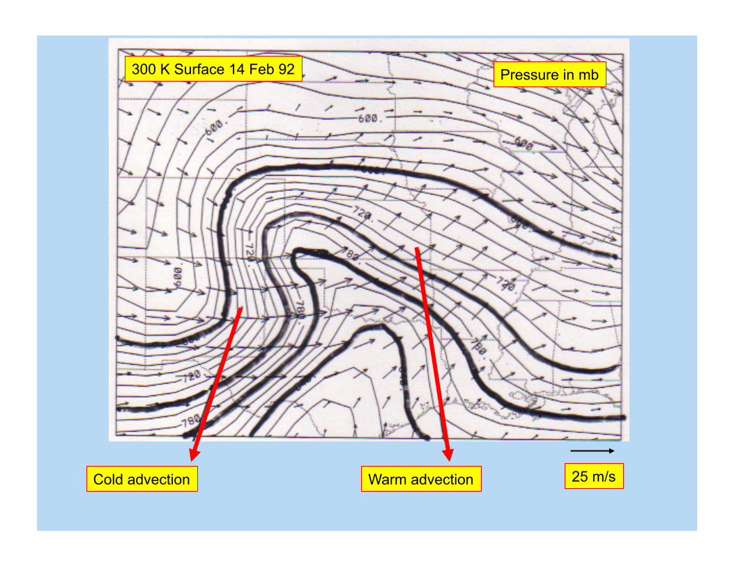
300 K Surface 14 Feb 92 Pressure in mb

25 m/s Cold advection Warm advection

€

ω =∂P∂t

⎛

⎝ ⎜

⎞

⎠ ⎟ θ

+ V •∇θ P +

∂P∂θ

dθdt

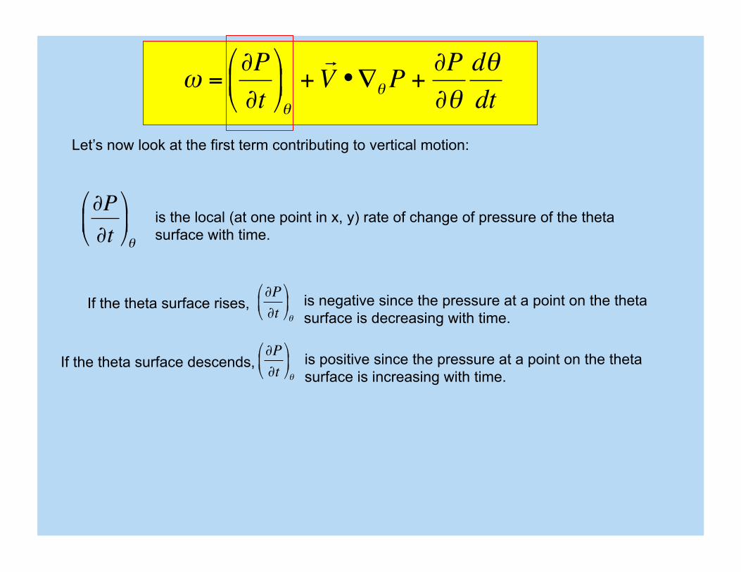
Let’s now look at the first term contributing to vertical motion:

€

∂P∂t

⎛

⎝ ⎜

⎞

⎠ ⎟ θ

is the local (at one point in x, y) rate of change of pressure of the theta surface with time.

If the theta surface rises,

€

∂P∂t

⎛

⎝ ⎜

⎞

⎠ ⎟ θ

is negative since the pressure at a point on the theta surface is decreasing with time.

If the theta surface descends,

€

∂P∂t

⎛

⎝ ⎜

⎞

⎠ ⎟ θ

is positive since the pressure at a point on the theta surface is increasing with time.

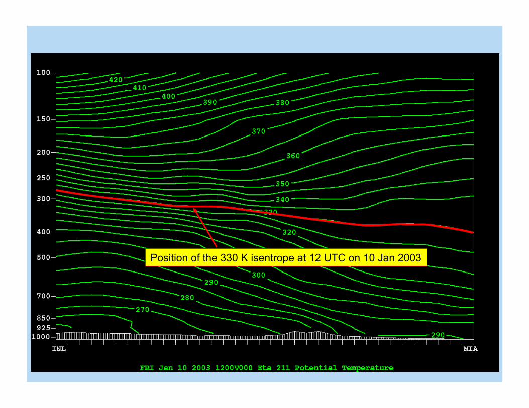
Position of the 330 K isentrope at 12 UTC on 10 Jan 2003

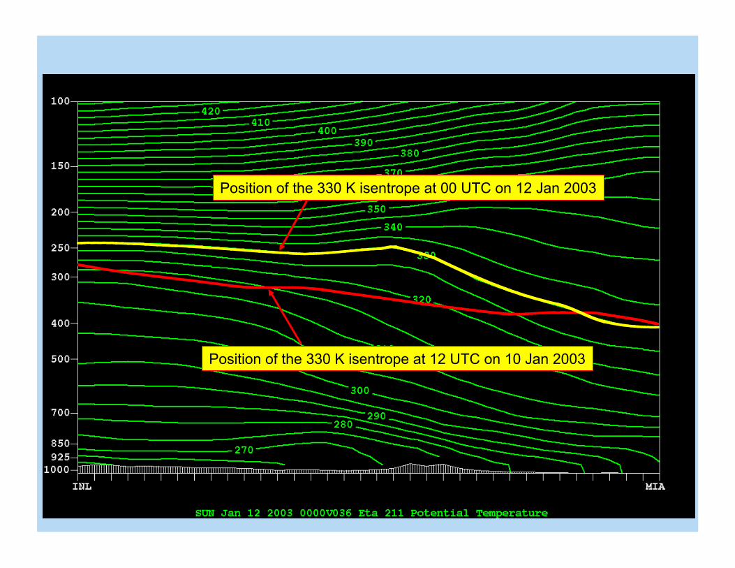
Position of the 330 K isentrope at 12 UTC on 10 Jan 2003

Position of the 330 K isentrope at 00 UTC on 12 Jan 2003

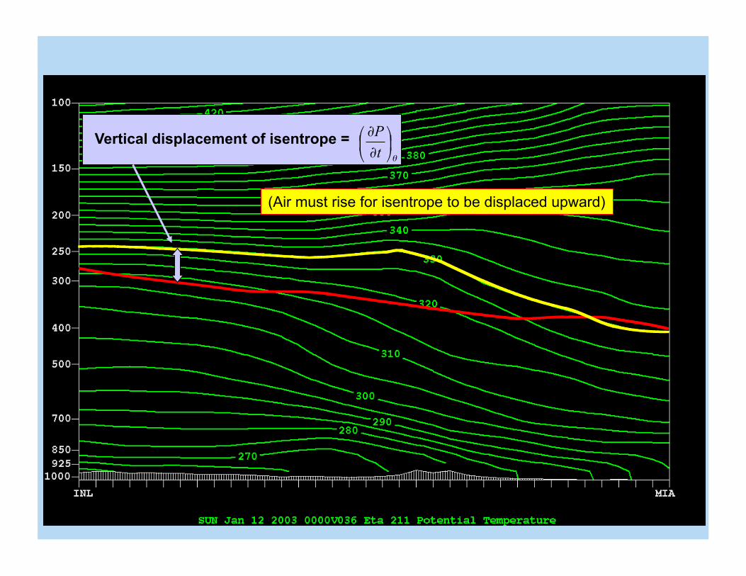
Vertical displacement of isentrope = θ

⎟⎠

⎞⎜⎝

⎛∂∂tP

(Air must rise for isentrope to be displaced upward)

dtdPPV

tP θ

θω θ

θ ∂∂

+∇•+⎟⎠

⎞⎜⎝

⎛∂∂

=

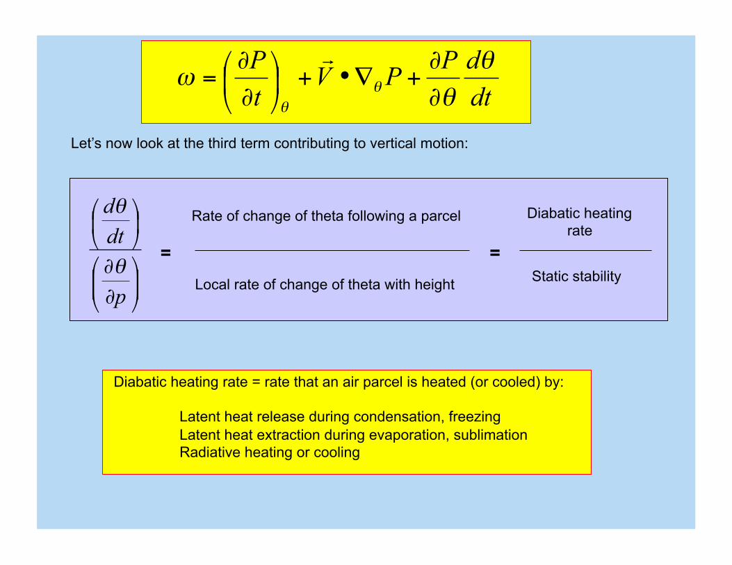
Let’s now look at the third term contributing to vertical motion:

⎟⎟⎠

⎞⎜⎜⎝

⎛

∂∂

⎟⎠

⎞⎜⎝

⎛

p

dtd

θ

θ Rate of change of theta following a parcel

Local rate of change of theta with height

= =

Diabatic heating rate

Static stability

Diabatic heating rate = rate that an air parcel is heated (or cooled) by:

Latent heat release during condensation, freezing Latent heat extraction during evaporation, sublimation Radiative heating or cooling

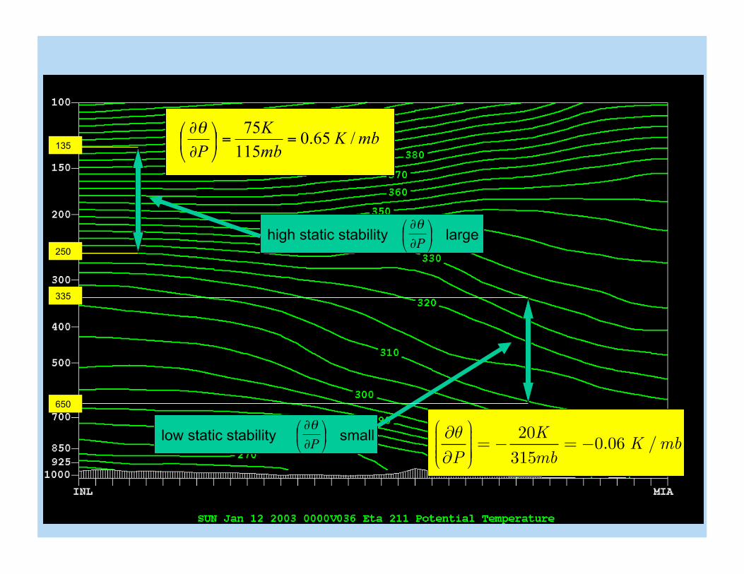
low static stability ⎟⎠

⎞⎜⎝

⎛∂∂Pθ

small

335

650

250

135

∂θ∂P

⎛

⎝⎜⎜⎜⎜

⎞

⎠⎟⎟⎟⎟⎟

= −20K

315mb= −0.06 K /mb

mbKmbK

P/65.0

11575

==⎟⎠

⎞⎜⎝

⎛∂∂θ

high static stability ⎟⎠

⎞⎜⎝

⎛∂∂Pθ

large

⎟⎟⎠

⎞⎜⎜⎝

⎛

∂∂

⎟⎠

⎞⎜⎝

⎛

p

dtd

θ

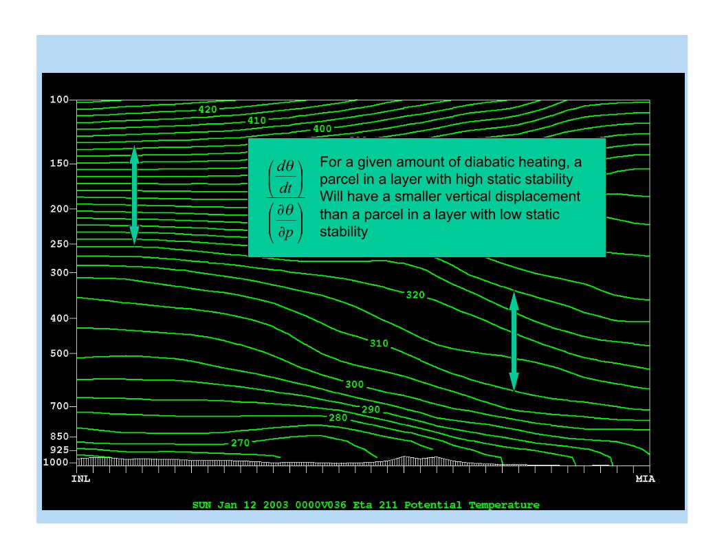
θ For a given amount of diabatic heating, a parcel in a layer with high static stability Will have a smaller vertical displacement than a parcel in a layer with low static stability

dtdPPV

tP θ

θω θ

θ ∂∂

+∇•+⎟⎠

⎞⎜⎝

⎛∂∂

=

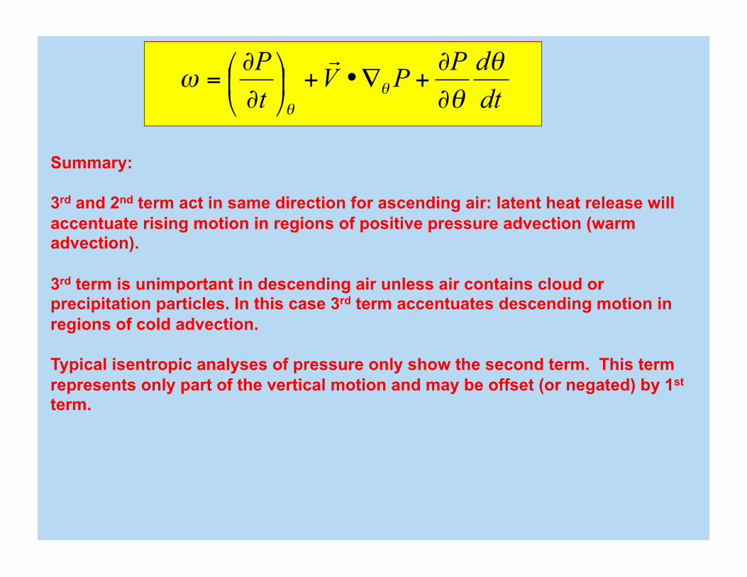
Summary:

3rd and 2nd term act in same direction for ascending air: latent heat release will accentuate rising motion in regions of positive pressure advection (warm advection).

3rd term is unimportant in descending air unless air contains cloud or precipitation particles. In this case 3rd term accentuates descending motion in regions of cold advection.

Typical isentropic analyses of pressure only show the second term. This term represents only part of the vertical motion and may be offset (or negated) by 1st term.

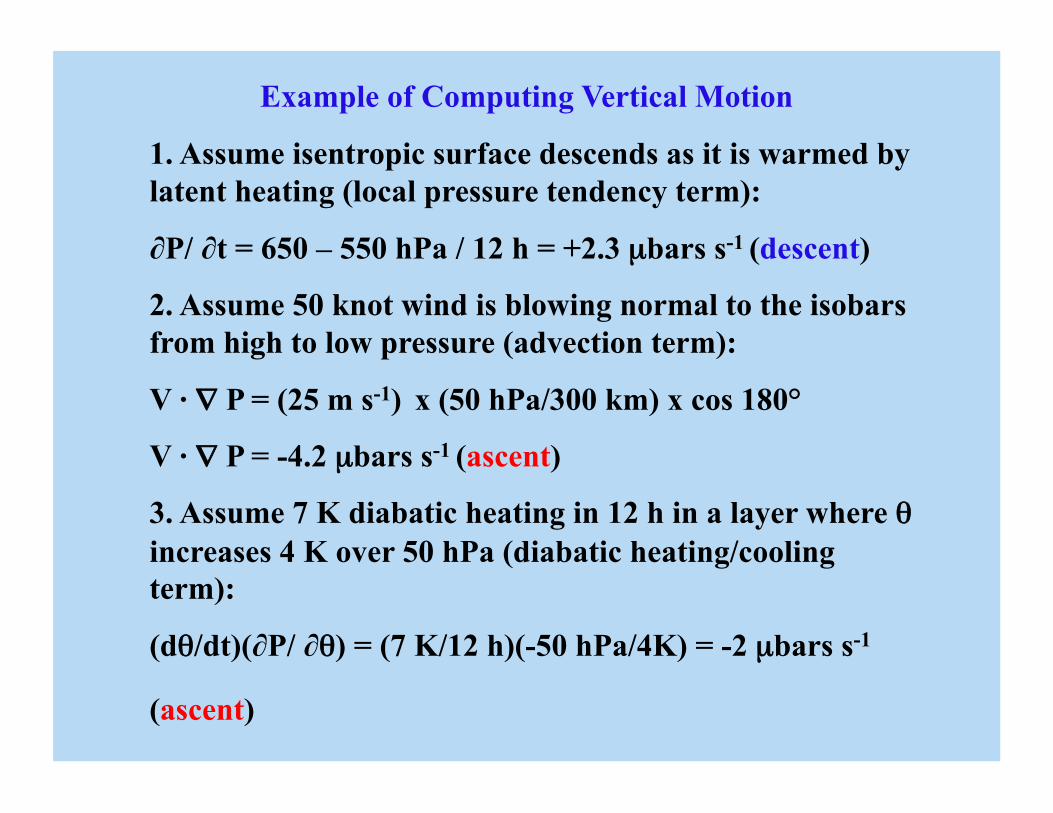
Example of Computing Vertical Motion

1. Assume isentropic surface descends as it is warmed by latent heating (local pressure tendency term):

∂P/ ∂t = 650 – 550 hPa / 12 h = +2.3 µbars s-1 (descent)

2. Assume 50 knot wind is blowing normal to the isobars from high to low pressure (advection term):

V · ∇ P = (25 m s-1) x (50 hPa/300 km) x cos 180°

V · ∇ P = -4.2 µbars s-1 (ascent)

3. Assume 7 K diabatic heating in 12 h in a layer where θ increases 4 K over 50 hPa (diabatic heating/cooling term):

(dθ/dt)(∂P/ ∂θ) = (7 K/12 h)(-50 hPa/4K) = -2 µbars s-1

(ascent)

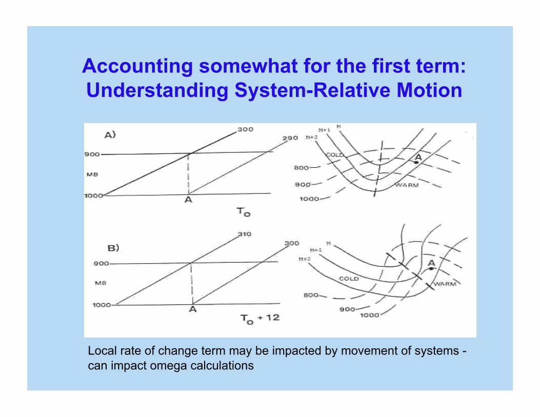
Accounting somewhat for the first term: Understanding System-Relative Motion

Local rate of change term may be impacted by movement of systems - can impact omega calculations

€

ω =∂P∂t

⎛

⎝ ⎜

⎞

⎠ ⎟ θ

+ V •∇θ P +

∂P∂θ

dθdt

€

ω =∂P∂t

⎛

⎝ ⎜

⎞

⎠ ⎟ θ

+ V •∇θ PNeglect diabatic processes

€

ω =∂P∂t

⎛

⎝ ⎜

⎞

⎠ ⎟ θ

+ V •∇θ P +

C •∇θ P −

C •∇θ P

€

ω =∂P∂t

⎛

⎝ ⎜

⎞

⎠ ⎟ θ

+ C •∇θ P +

V − C ( ) •∇θ P

Add and subtract advection by system

Rearrange

Vertical motion using system relative winds

System tendency: If the system is neither deepening, filling, or reorienting, term 1 will balance 2 in yellow box so that yellow box = 0

€

ω* =

V − C ( ) •∇θ P

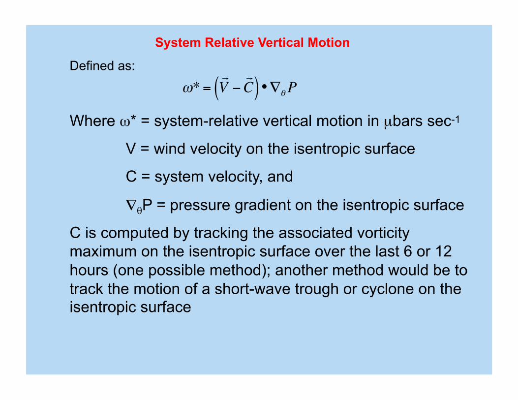
Defined as:

Where ω* = system-relative vertical motion in µbars sec-1

V = wind velocity on the isentropic surface

C = system velocity, and

∇θP = pressure gradient on the isentropic surface

C is computed by tracking the associated vorticity maximum on the isentropic surface over the last 6 or 12 hours (one possible method); another method would be to track the motion of a short-wave trough or cyclone on the isentropic surface

System Relative Vertical Motion

€

ω* =

V − C ( ) •∇θ P

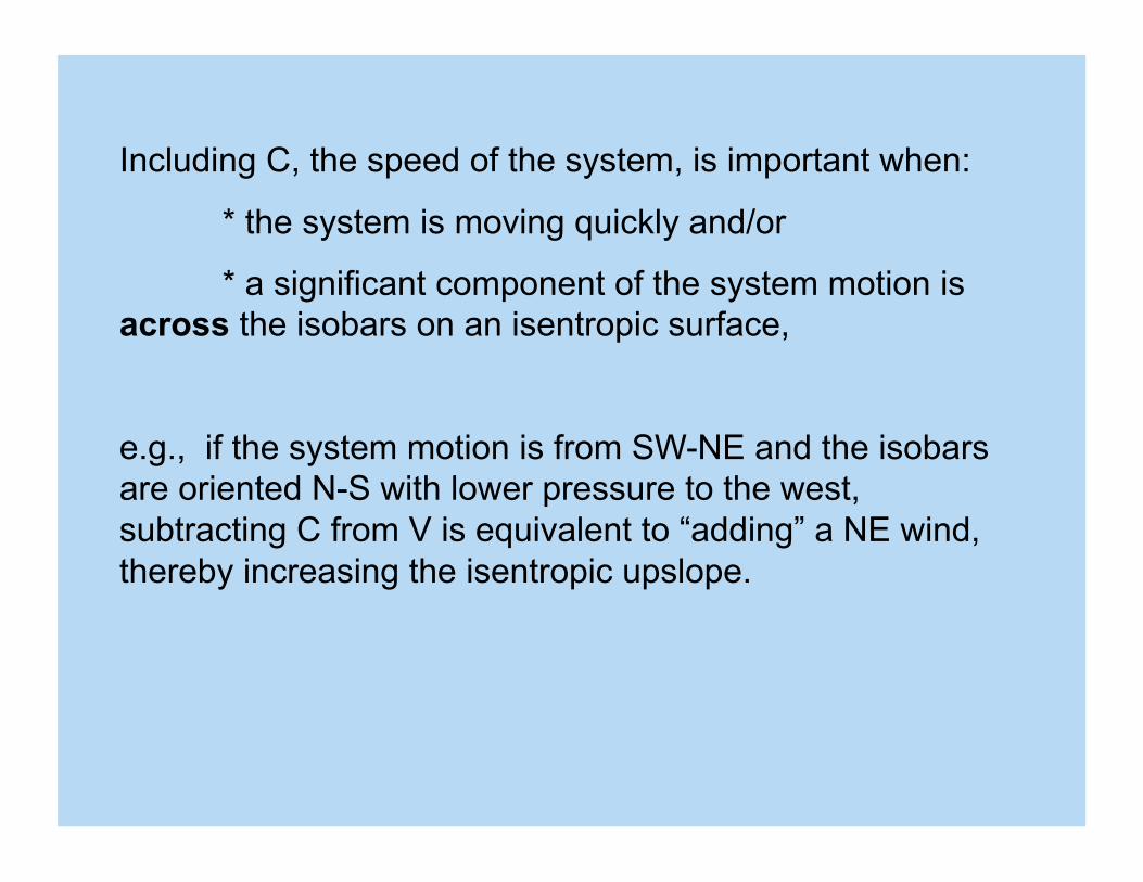
Including C, the speed of the system, is important when:

* the system is moving quickly and/or

* a significant component of the system motion is across the isobars on an isentropic surface,

e.g., if the system motion is from SW-NE and the isobars are oriented N-S with lower pressure to the west, subtracting C from V is equivalent to “adding” a NE wind, thereby increasing the isentropic upslope.

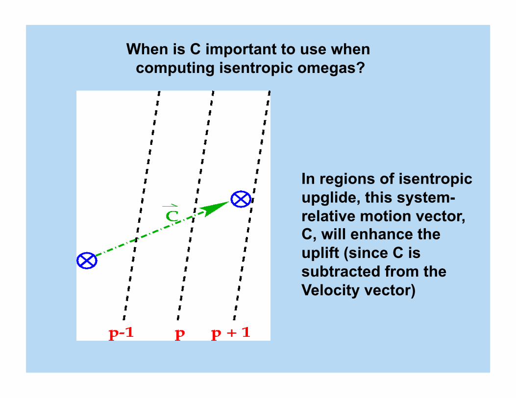
In regions of isentropic upglide, this system-relative motion vector, C, will enhance the uplift (since C is subtracted from the Velocity vector)

When is C important to use when computing isentropic omegas?

€

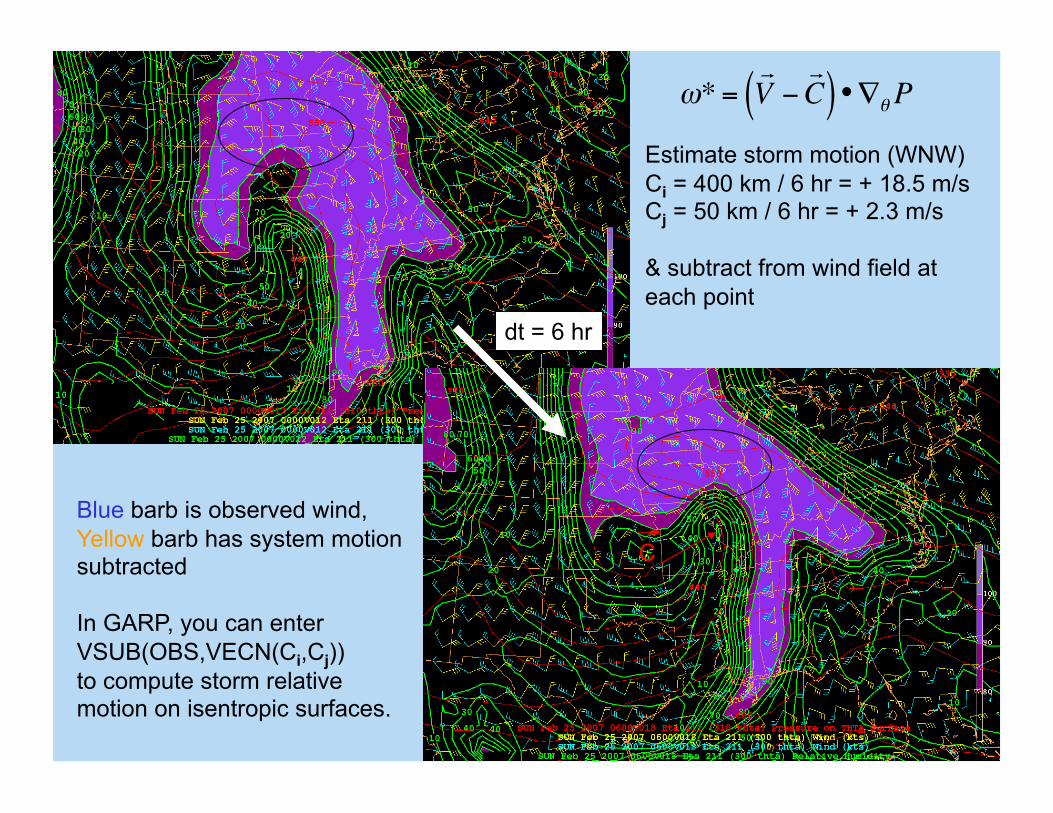
ω* =

V − C ( ) •∇θ P

Estimate storm motion (WNW) Ci = 400 km / 6 hr = + 18.5 m/s Cj = 50 km / 6 hr = + 2.3 m/s

& subtract from wind field at each point

Blue barb is observed wind, Yellow barb has system motion subtracted

In GARP, you can enter VSUB(OBS,VECN(Ci,Cj)) to compute storm relative motion on isentropic surfaces.

dt = 6 hr

C

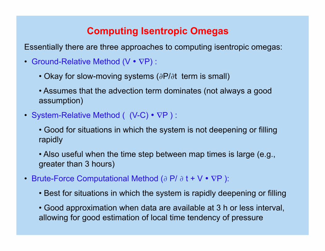
Computing Isentropic Omegas Essentially there are three approaches to computing isentropic omegas:

•  Ground-Relative Method (V • ∇P) :

•  Okay for slow-moving systems (∂P/∂t term is small)

•  Assumes that the advection term dominates (not always a good assumption)

•  System-Relative Method ( (V-C) • ∇P ) :

•  Good for situations in which the system is not deepening or filling rapidly

•  Also useful when the time step between map times is large (e.g., greater than 3 hours)

•  Brute-Force Computational Method (∂ P/ ∂ t + V • ∇P ):

•  Best for situations in which the system is rapidly deepening or filling

•  Good approximation when data are available at 3 h or less interval, allowing for good estimation of local time tendency of pressure

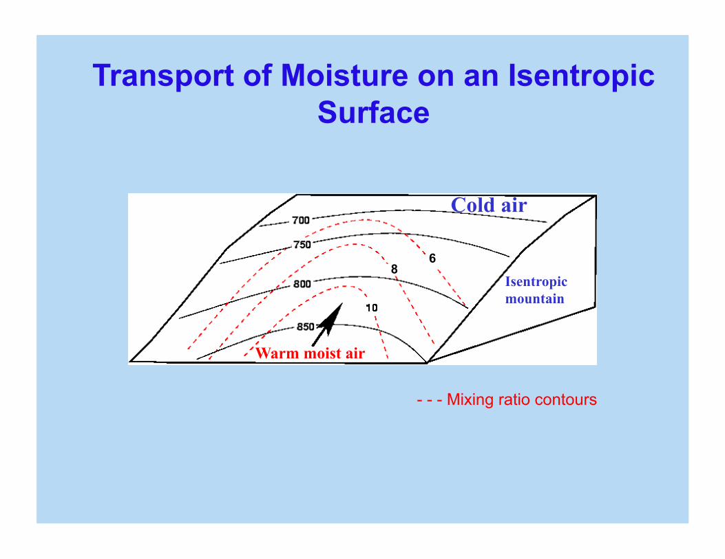
Transport of Moisture on an Isentropic Surface

8 6

Isentropicmountain

Warm moist air

Cold air

- - - Mixing ratio contours

System-Relative Flow: How can it be used? Carlson (1991, Mid-Latitude Weather Systems) notes:

•  Relative-wind analysis reveals the existence of sharply-defined boundaries, which differentiate air streams of vastly differing moisture contents. Air streams tend to contain relatively narrow ranges of θ and θe peeculiar to the air stream’s origins.

•  Relative-wind isentropic analyses for synoptic-scale weather systems tend to show well-defined air streams, which have been identified by the names – warm conveyor belt, cold conveyor belt and dry conveyor belt.

•  Thus, a conveyor belt consists of an ensemble of air parcels having nearly the same θ (or θe) value, starting from a common initial location, which travel over synoptic-scale time periods (> 18 h).

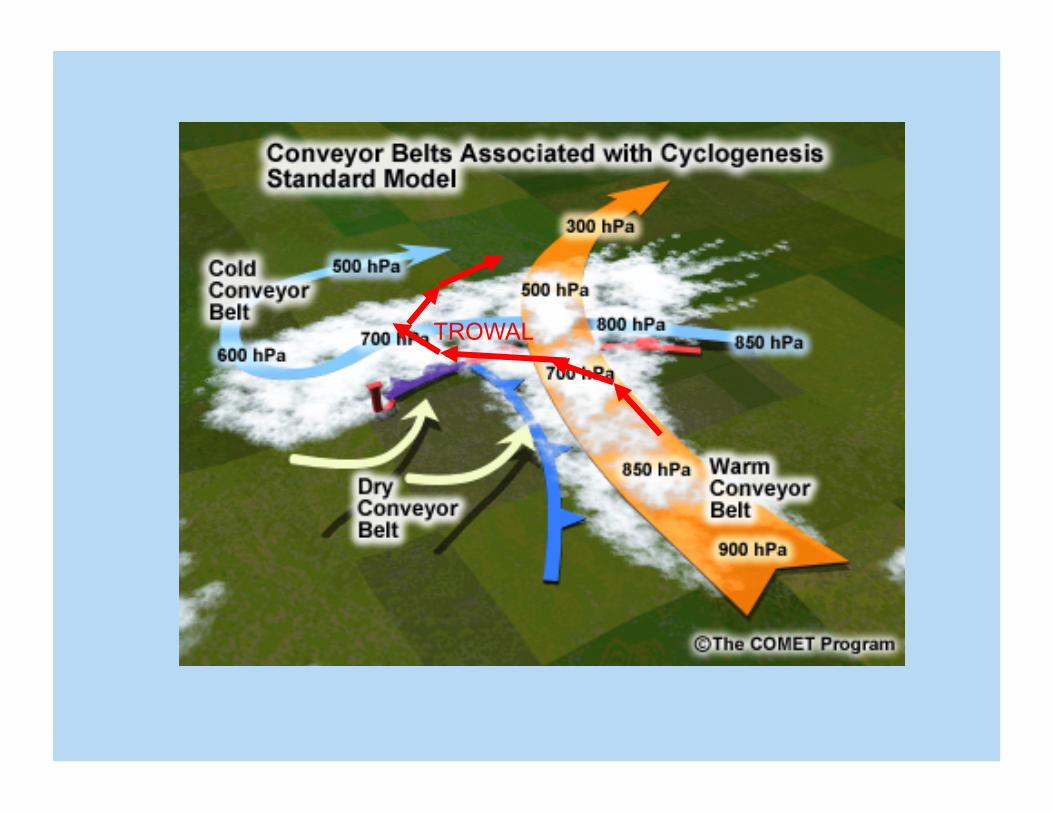
TROWAL

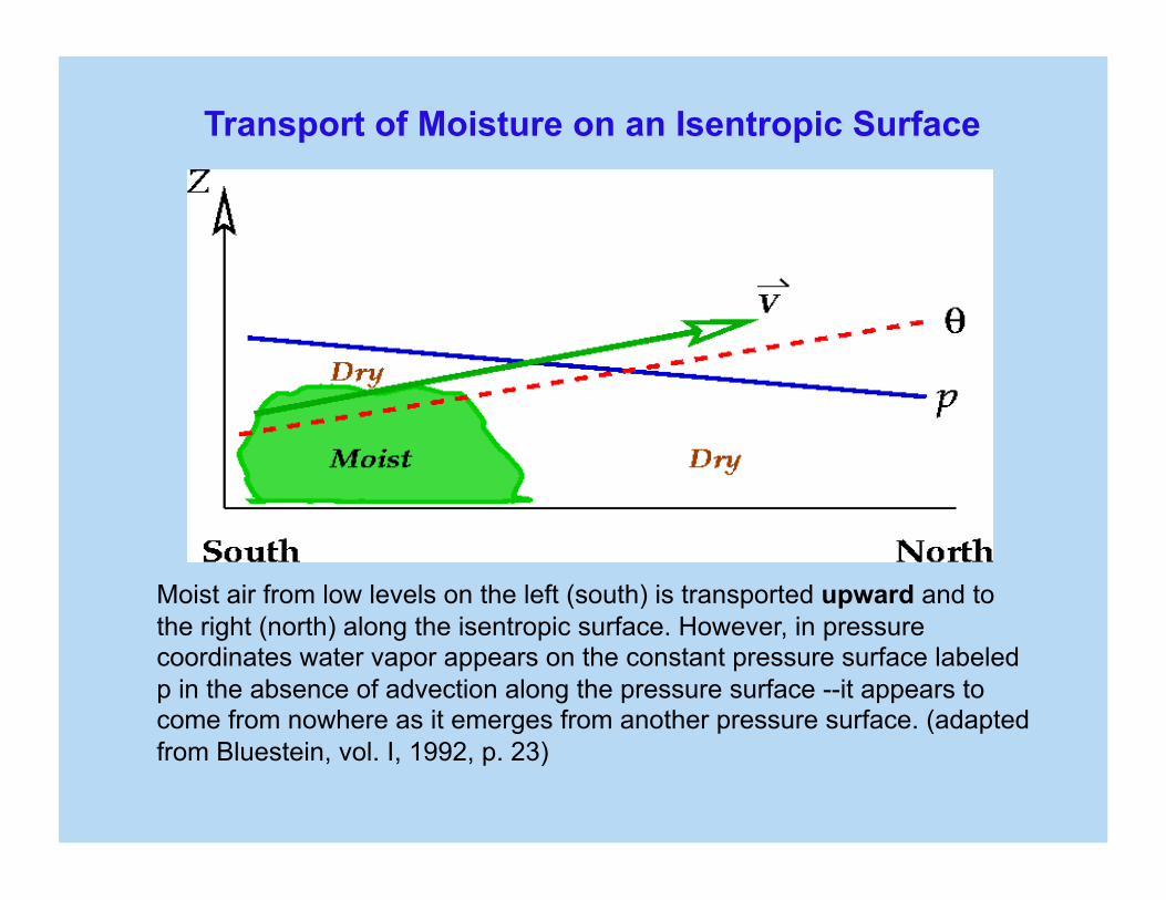
Transport of Moisture on an Isentropic Surface

Moist air from low levels on the left (south) is transported upward and to the right (north) along the isentropic surface. However, in pressure coordinates water vapor appears on the constant pressure surface labeled p in the absence of advection along the pressure surface --it appears to come from nowhere as it emerges from another pressure surface. (adapted from Bluestein, vol. I, 1992, p. 23)

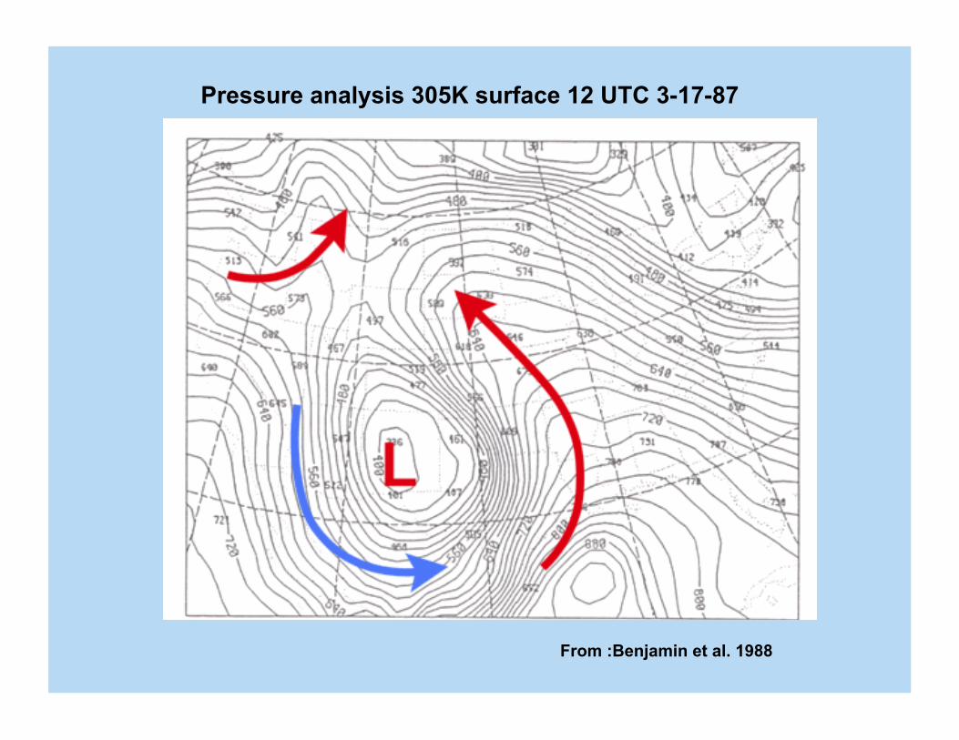
Pressure analysis 305K surface 12 UTC 3-17-87

From :Benjamin et al. 1988

Relative Humidity 305K surface 12 UTC 3-17-87 RH>80% = green

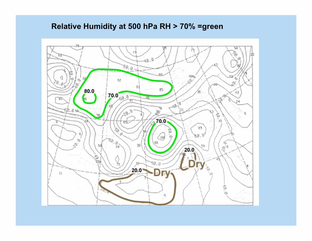
Relative Humidity at 500 hPa RH > 70% =green

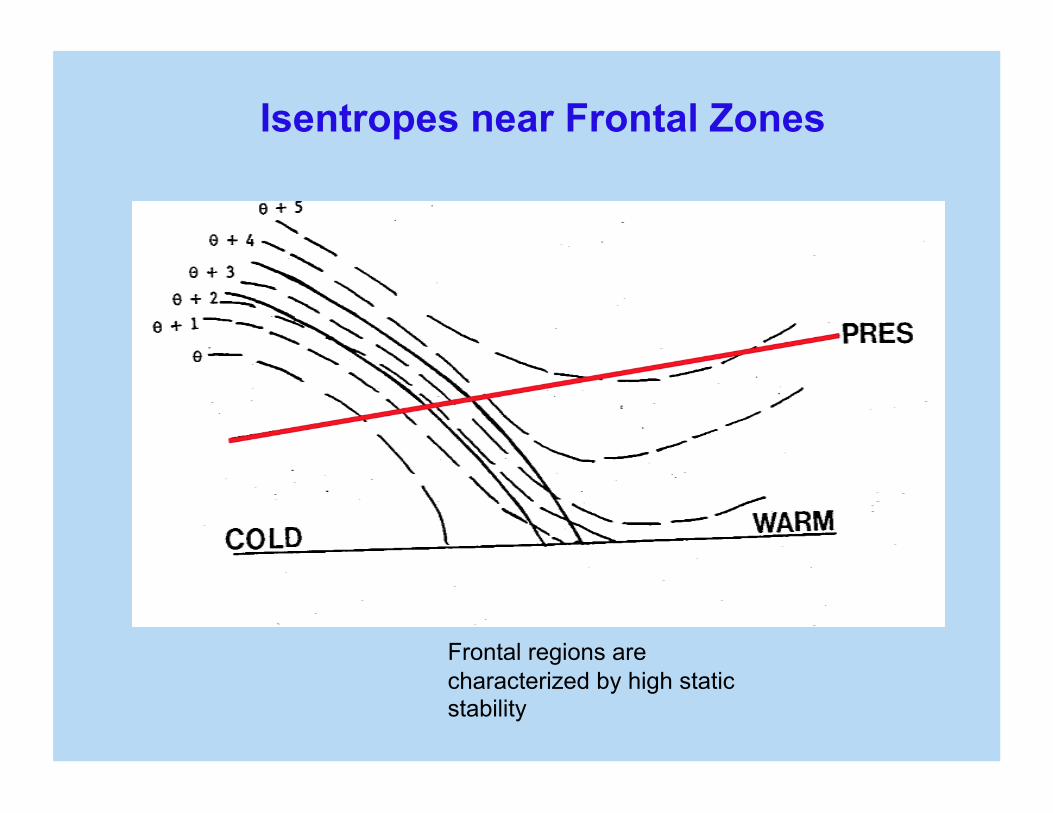
Isentropes near Frontal Zones

Frontal regions are characterized by high static stability

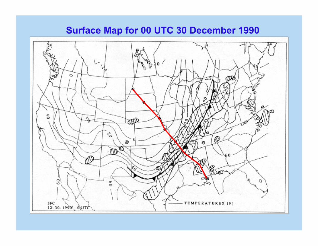
Surface Map for 00 UTC 30 December 1990

Surface Map for 12 UTC 30 December 1990

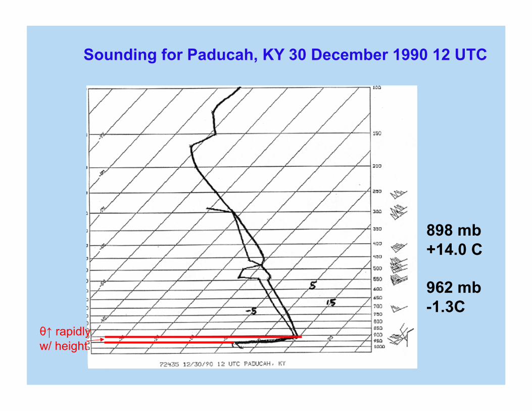
898 mb +14.0 C

962 mb -1.3C

Sounding for Paducah, KY 30 December 1990 12 UTC

θ↑ rapidly w/ height

Cross Section Taken Normal to Arctic Frontal Zone: 12 UTC 30 December 1990

∂θ/∂z >> 0 - very stable!

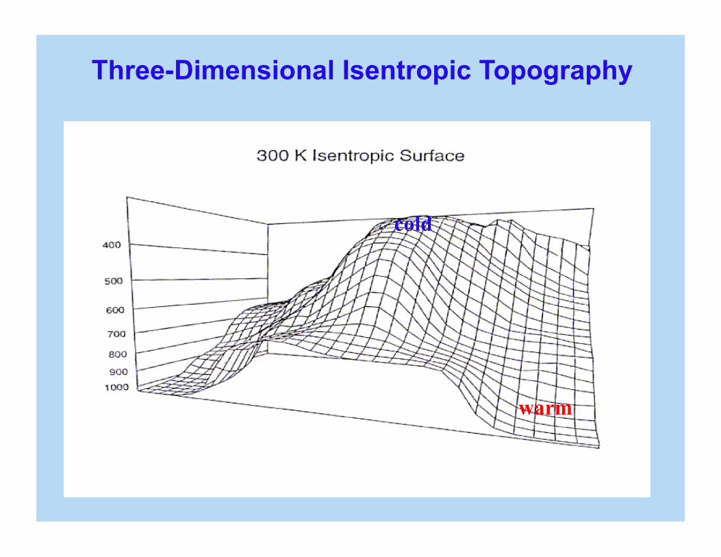
Three-Dimensional Isentropic Topography

warm

cold

( ) dzzPdy

yPdx

xPdP

yxxzyz ,,,⎟⎠

⎞⎜⎝

⎛∂∂

+⎟⎟⎠

⎞⎜⎜⎝

⎛

∂∂

+⎟⎠

⎞⎜⎝

⎛∂∂

=θ

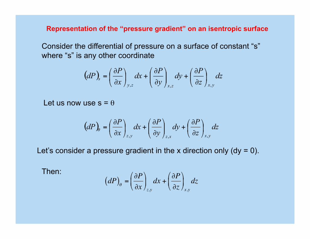
Representation of the “pressure gradient” on an isentropic surface

Consider the differential of pressure on a surface of constant “s” where “s” is any other coordinate

( ) dzzPdy

yPdx

xPdP

yxzxzys

,,,⎟⎠

⎞⎜⎝

⎛∂

∂+⎟⎟

⎠

⎞⎜⎜⎝

⎛

∂

∂+⎟

⎠

⎞⎜⎝

⎛∂

∂=

Let us now use s = θ

Let’s consider a pressure gradient in the x direction only (dy = 0).

Then:

€

dP( )θ =∂P∂x⎛

⎝ ⎜

⎞

⎠ ⎟ z,y

dx +∂P∂z

⎛

⎝ ⎜

⎞

⎠ ⎟ x,y

dz

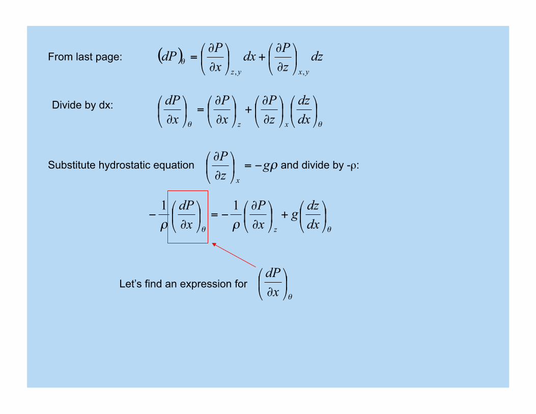
( ) dzzPdx

xPdP

yxyz ,,⎟⎠

⎞⎜⎝

⎛∂

∂+⎟

⎠

⎞⎜⎝

⎛∂

∂=θFrom last page:

Divide by dx:

θθ

⎟⎠

⎞⎜⎝

⎛⎟⎠

⎞⎜⎝

⎛∂

∂+⎟

⎠

⎞⎜⎝

⎛∂

∂=⎟

⎠

⎞⎜⎝

⎛∂ dx

dzzP

xP

xdP

xz

Substitute hydrostatic equation and divide by -ρ: ρgzP

x

−=⎟⎠

⎞⎜⎝

⎛∂

∂

θθ ρρ⎟⎠

⎞⎜⎝

⎛+⎟⎠

⎞⎜⎝

⎛∂

∂−=⎟

⎠

⎞⎜⎝

⎛∂

−dxdzg

xP

xdP

z

11

Let’s find an expression for θ

⎟⎠

⎞⎜⎝

⎛∂xdP

€

θ = T 1000P

⎛

⎝ ⎜

⎞

⎠ ⎟

RdC p

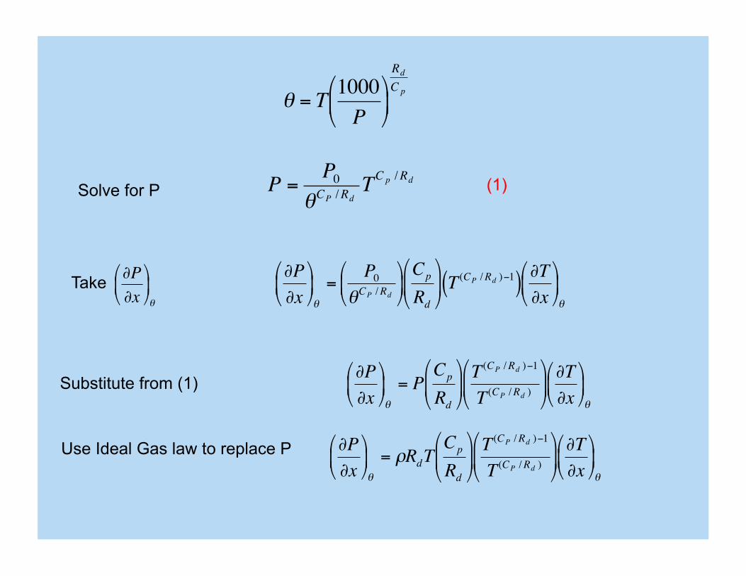
Solve for P

€

P =P0

θCP /RdTCp /Rd

Take

€

∂P∂x⎛

⎝ ⎜

⎞

⎠ ⎟ θ

€

∂P∂x⎛

⎝ ⎜

⎞

⎠ ⎟ θ

=P0

θCP /Rd

⎛

⎝ ⎜

⎞

⎠ ⎟ Cp

Rd

⎛

⎝ ⎜

⎞

⎠ ⎟ T (CP /Rd )−1( ) ∂T

∂x⎛

⎝ ⎜

⎞

⎠ ⎟ θ

(1)

Substitute from (1)

€

∂P∂x⎛

⎝ ⎜

⎞

⎠ ⎟ θ

= PCp

Rd

⎛

⎝ ⎜

⎞

⎠ ⎟ T (CP /Rd )−1

T (CP /Rd )

⎛

⎝ ⎜

⎞

⎠ ⎟ ∂T∂x⎛

⎝ ⎜

⎞

⎠ ⎟ θ

Use Ideal Gas law to replace P

€

∂P∂x⎛

⎝ ⎜

⎞

⎠ ⎟ θ

= ρRdTCp

Rd

⎛

⎝ ⎜

⎞

⎠ ⎟ T (CP /Rd )−1

T (CP /Rd )

⎛

⎝ ⎜

⎞

⎠ ⎟ ∂T∂x⎛

⎝ ⎜

⎞

⎠ ⎟ θ

€

∂P∂x⎛

⎝ ⎜

⎞

⎠ ⎟ θ

= ρRdTCp

Rd

⎛

⎝ ⎜

⎞

⎠ ⎟ T (CP /Rd )−1

T (CP /Rd )

⎛

⎝ ⎜

⎞

⎠ ⎟ ∂T∂x⎛

⎝ ⎜

⎞

⎠ ⎟ θ

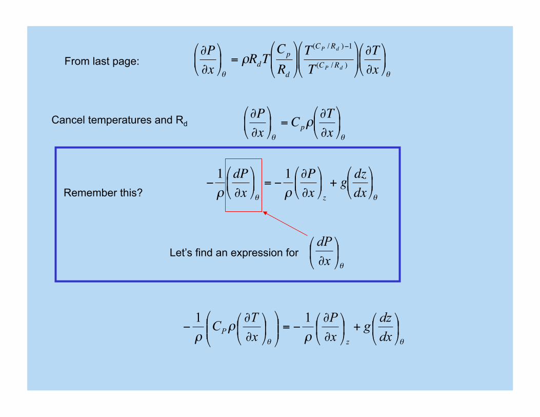
From last page:

Cancel temperatures and Rd

€

∂P∂x⎛

⎝ ⎜

⎞

⎠ ⎟ θ

= Cpρ∂T∂x⎛

⎝ ⎜

⎞

⎠ ⎟ θ

Remember this?

€

−1ρ

dP∂x

⎛

⎝ ⎜

⎞

⎠ ⎟ θ

= −1ρ∂P∂x⎛

⎝ ⎜

⎞

⎠ ⎟ z

+ g dzdx⎛

⎝ ⎜

⎞

⎠ ⎟ θ

Let’s find an expression for θ

⎟⎠

⎞⎜⎝

⎛∂xdP

θθ ρρ

ρ⎟⎠

⎞⎜⎝

⎛+⎟⎠

⎞⎜⎝

⎛∂

∂−=⎟⎟

⎠

⎞⎜⎜⎝

⎛⎟⎠

⎞⎜⎝

⎛∂

∂−

dxdzg

xP

xTC

zP

11

θθ ρρ

ρ⎟⎠

⎞⎜⎝

⎛+⎟⎠

⎞⎜⎝

⎛∂

∂−=⎟⎟

⎠

⎞⎜⎜⎝

⎛⎟⎠

⎞⎜⎝

⎛∂

∂−

dxdzg

xP

xTC

zP

11

Rearrange: ( )θρ⎟⎠

⎞⎜⎝

⎛ +−=⎟⎠

⎞⎜⎝

⎛∂

∂− gzTC

dxd

xP

pz

1

Or: θρ⎟⎠

⎞⎜⎝

⎛−=⎟⎠

⎞⎜⎝

⎛∂

∂−

dxdM

xP

z

1

Similarly: θ

ρ ⎟⎟⎠

⎞⎜⎜⎝

⎛−=⎟⎟

⎠

⎞⎜⎜⎝

⎛

∂

∂−

dydM

yP

z

1

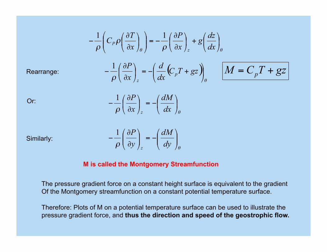
M is called the Montgomery Streamfunction

The pressure gradient force on a constant height surface is equivalent to the gradient Of the Montgomery streamfunction on a constant potential temperature surface.

Therefore: Plots of M on a potential temperature surface can be used to illustrate the pressure gradient force, and thus the direction and speed of the geostrophic flow.

gzTCM p +=

Depicting geostrophic flow on an isentropic surface:

On a pressure surface, the geostrophic flow is depicted by height contours, where the geostrophic wind is parallel to the height contours, and its magnitude is proportional to the spacing of the contours

On an isentropic surface, the geostrophic flow is depicted by contours of the Montgomery streamfunction, where the geostrophic wind is parallel to the contours of the Montgomery Streamfunction and is proportional to their spacing.

gzTCM p +=

€

Vg = 1f

ˆ k ×∇θMθρ ⎟⎟

⎠

⎞⎜⎜⎝

⎛−=⎟⎟

⎠

⎞⎜⎜⎝

⎛

∂

∂−

dydM

yP

z

1Since It follows that

€

Vg = 1fρ

ˆ k ×∇ z pand

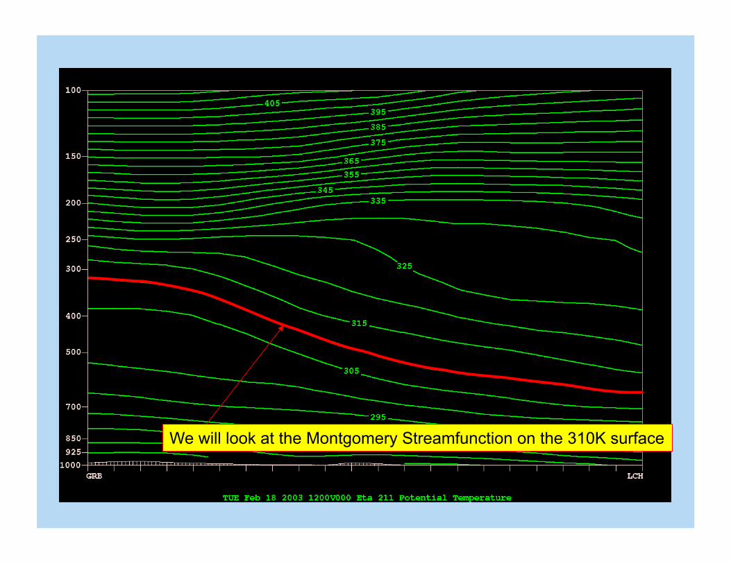
We will look at the Montgomery Streamfunction on the 310K surface

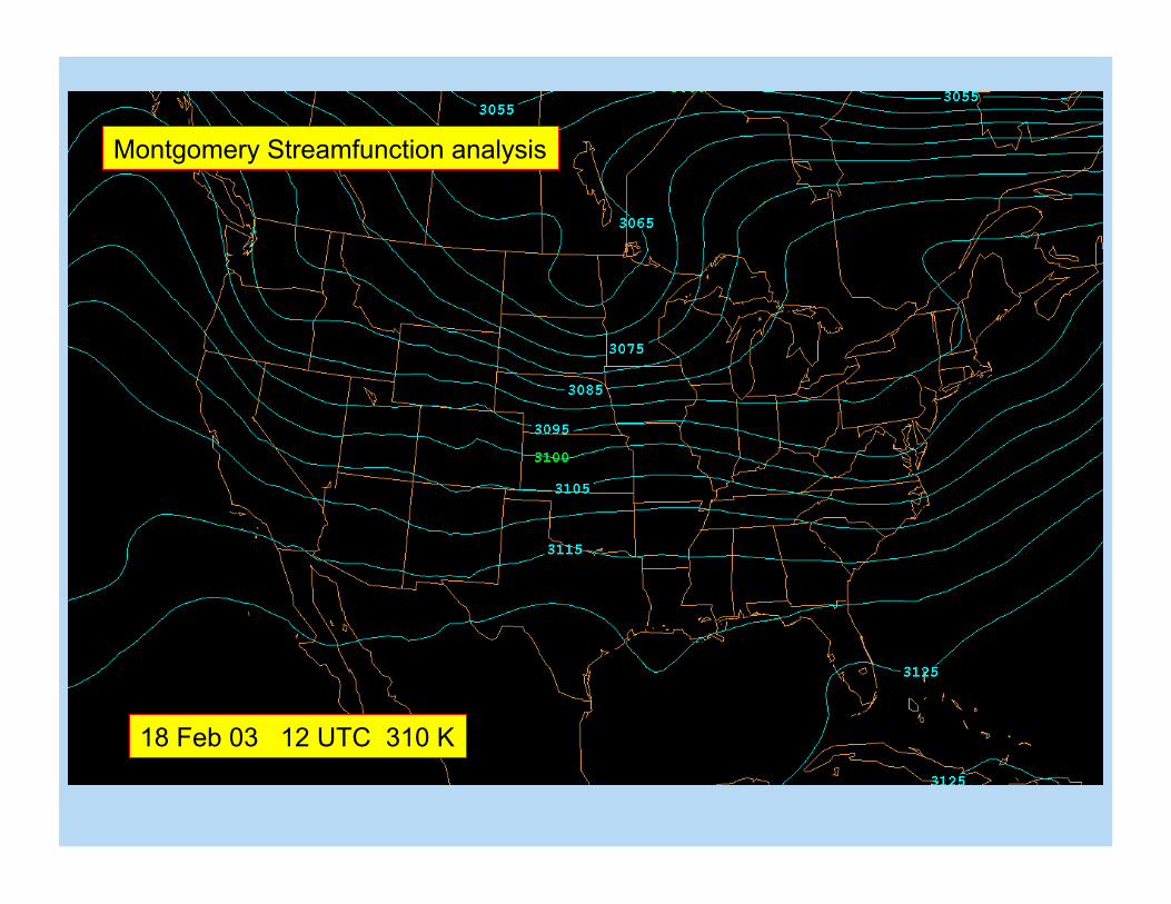
Montgomery Streamfunction analysis

18 Feb 03 12 UTC 310 K

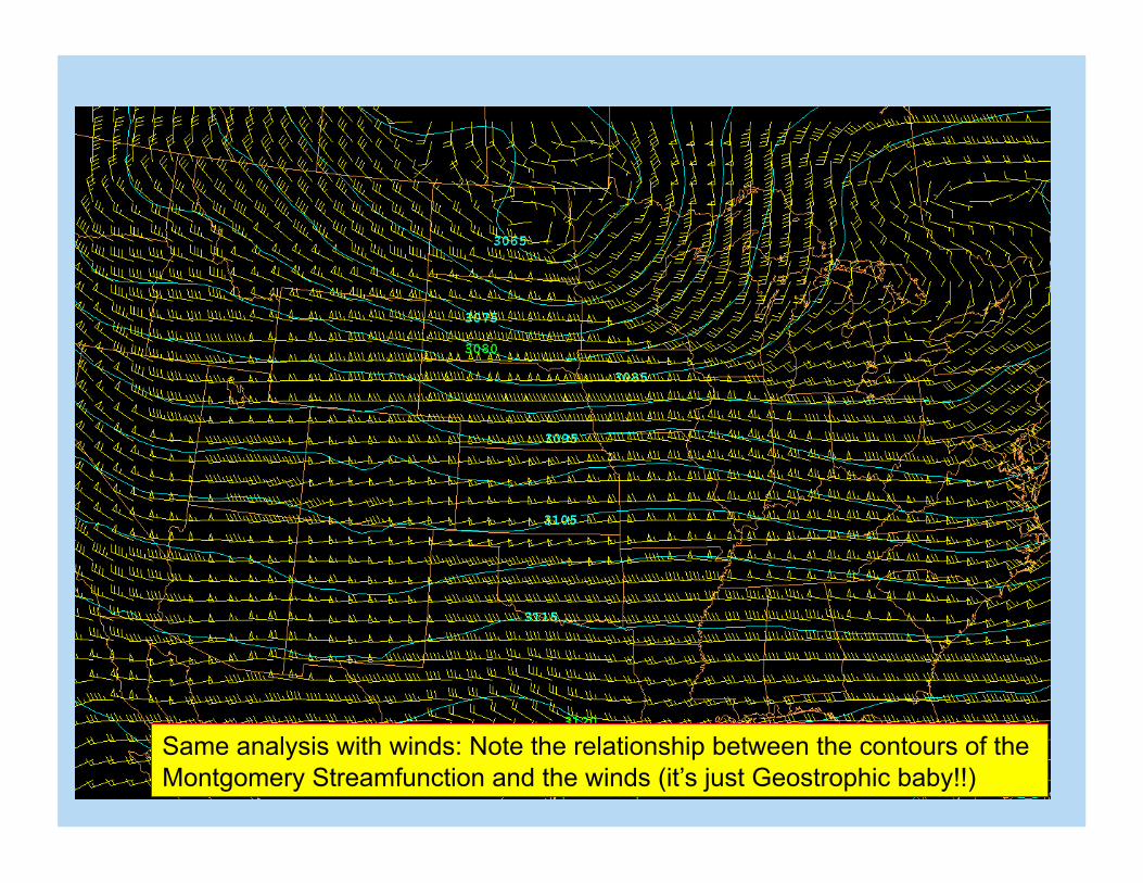
Same analysis with winds: Note the relationship between the contours of the Montgomery Streamfunction and the winds (it’s just Geostrophic baby!!)

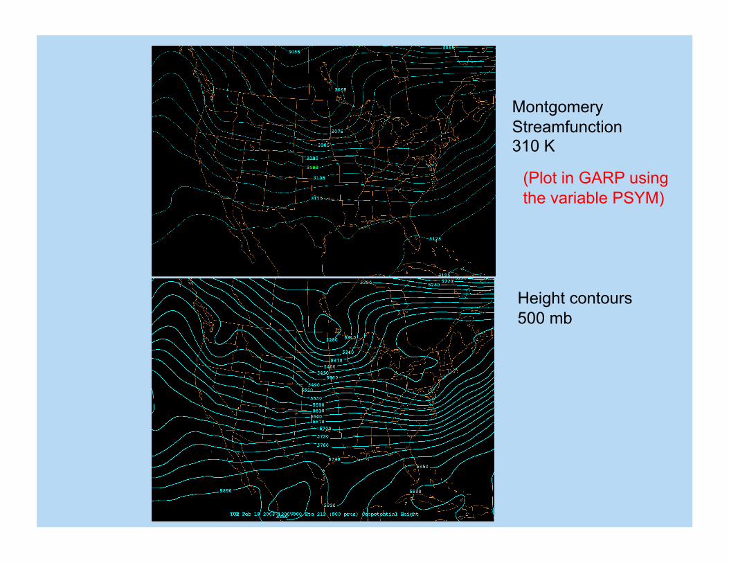
Montgomery Streamfunction 310 K

Height contours 500 mb

(Plot in GARP using the variable PSYM)

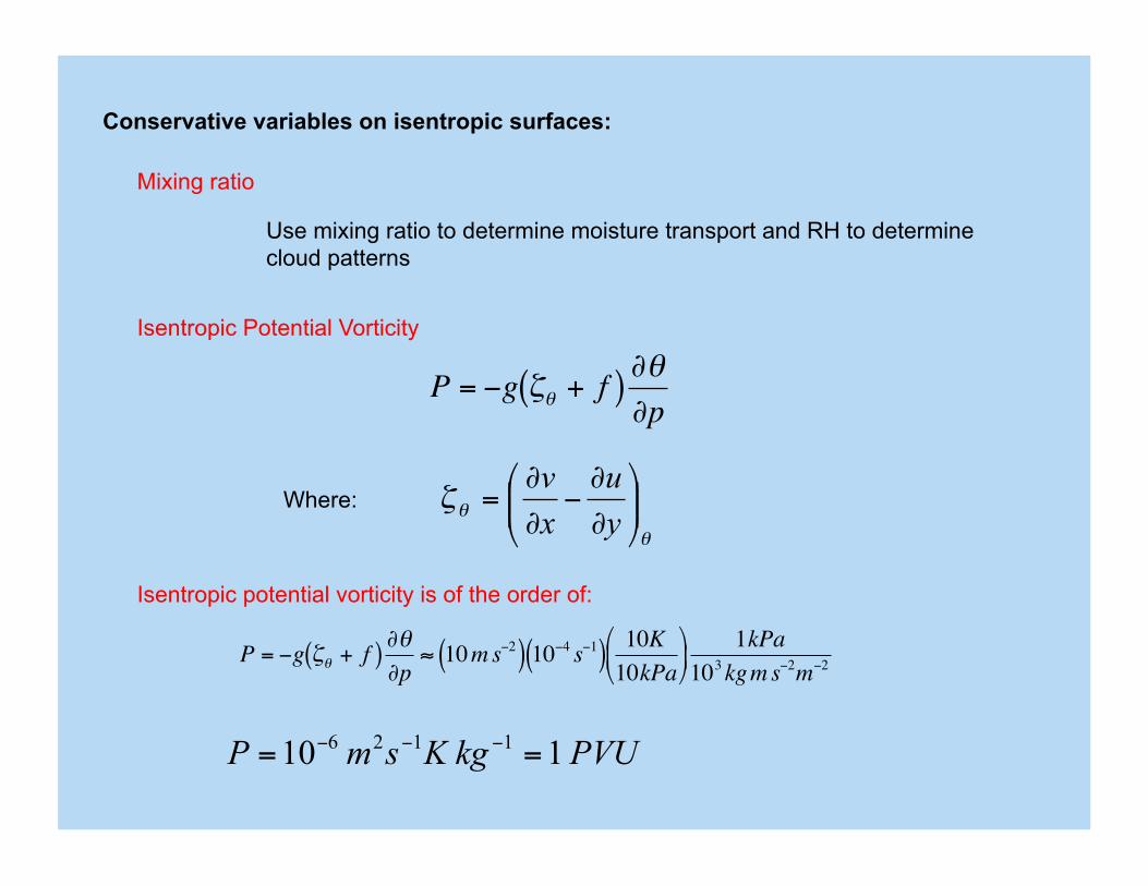
Conservative variables on isentropic surfaces:

Use mixing ratio to determine moisture transport and RH to determine cloud patterns

Mixing ratio

Isentropic Potential Vorticity

€

P = −g ζθ + f( ) ∂θ∂p

θ

θζ ⎟⎟⎠

⎞⎜⎜⎝

⎛

∂

∂−

∂

∂=

yu

xv

Where:

€

P = −g ζθ + f( ) ∂θ∂p

≈ 10ms−2( ) 10−4 s−1( ) 10K10kPa⎛

⎝ ⎜

⎞

⎠ ⎟

1kPa103kgm s−2m−2

Isentropic potential vorticity is of the order of:

PVUkgKsmP 110 1126 == −−−

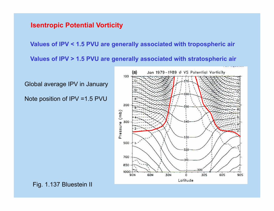
Isentropic Potential Vorticity

Values of IPV < 1.5 PVU are generally associated with tropospheric air

Values of IPV > 1.5 PVU are generally associated with stratospheric air

Fig. 1.137 Bluestein II

Global average IPV in January

Note position of IPV =1.5 PVU

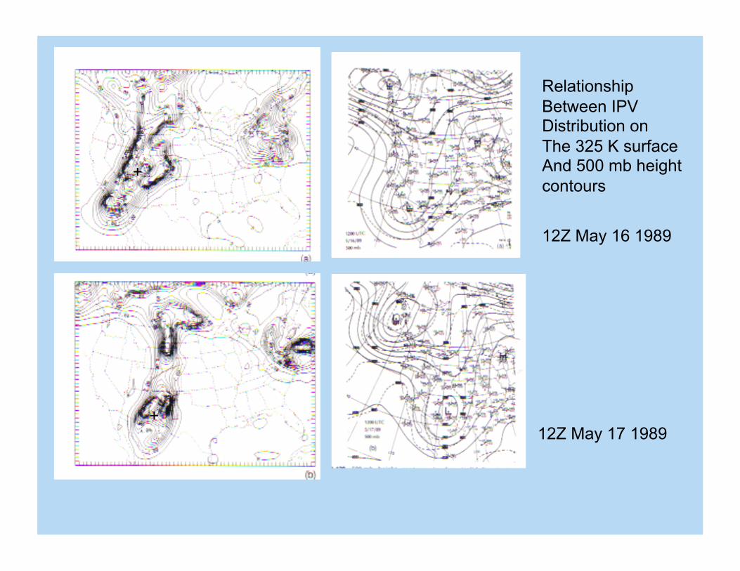
Relationship Between IPV Distribution on The 325 K surface And 500 mb height contours

12Z May 16 1989

12Z May 17 1989

+

+

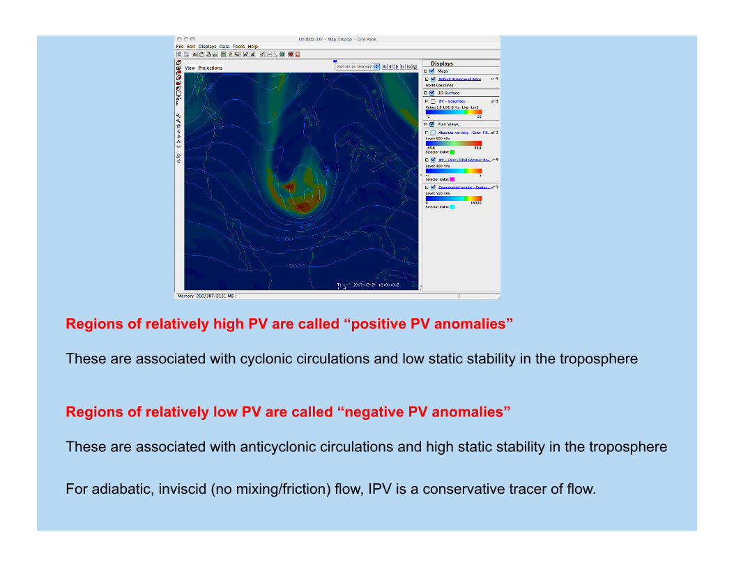
Regions of relatively high PV are called “positive PV anomalies”

These are associated with cyclonic circulations and low static stability in the troposphere

Regions of relatively low PV are called “negative PV anomalies”

These are associated with anticyclonic circulations and high static stability in the troposphere

For adiabatic, inviscid (no mixing/friction) flow, IPV is a conservative tracer of flow.

IPV has come into use in forecasting because of its invertibility:

If one assumes a balance condition (e.g. geostrophic balance, gradient wind balance or higher order balances), specification of the IPV field allows one to deduce the pressure and wind fields. Why do these assumptions allow you to use only IPV to determine the state of the atmosphere?

We will learn more about IPV later on in this course!

€

P = −g ζθ + f( ) ∂θ∂p

Isentropic Analysis: Advantages •  For synoptic scale motions, in the absence of diabatic processes, isentropic surfaces are material surfaces, i.e., parcels are thermodynamically bound to the surface. •  Horizontal flow along an isentropic surface contains the adiabatic component of vertical motion. •  Moisture transport on an isentropic surface is three-dimensional - patterns are more spatially and temporally coherent than on pressure surfaces. •  Isentropic surfaces tend to run parallel to frontal zones making the variation of basic quantities (u,v, T, q) more gradual along them.

Isentropic Analysis: Advantages

•  Atmospheric variables tend to be better correlated along an isentropic surface upstream/downstream, than on a constant pressure surface, especially in advective flow

•  The vertical spacing between isentropic surfaces is a measure of the dry static stability. Divergence (convergence) between two isentropic surfaces decreases (increases) the static stability in the layer.

•  The slope of an isentropic surface (or pressure gradient along it) is directly related to the thermal wind.

•  Parcel trajectories can easily be computed on an isentropic surface. Lagrangian (parcel) vertical motion fields are better correlated to satellite imagery than Eulerian (instantaneous) vertical motion fields.

Isentropic Analysis: Disadvantages

•  In areas of neutral or superadiabatic lapse rates isentropic surfaces are ill-defined, i.e., they are multi-valued with respect to pressure;

•  In areas of near-neutral lapse rates there is poor vertical resolution of atmospheric features. In stable frontal zones, however there is excellent vertical resolution.

•  Diabatic processes significantly disrupt the continuity of isentropic surfaces. Major diabatic processes include: latent heating/evaporative cooling, solar heating, and infrared cooling.

•  Isentropic surfaces tend to intersect the ground at steep angles (e.g., SW U.S.) require careful analysis there.

Isentropic Analysis: Disadvantages

• The “proper” isentropic surface to analyze on a given day varies with season, latitude, and time of day. There are no fixed levels to analyze (e.g., 500 hPa) as with constant pressure analysis.

• If we practice “meteorological analysis” the above disadvantage turns into an advantage since we must think through what we are looking for and why!