ISE 195Introduction to Industrial

Engineering

Lecture 3

Mathematical Optimization

(Topics in ISE 470 Deterministic Operations Research

Models)

3

What is “OR”?

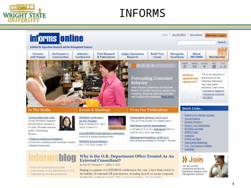
“Operations Research” = “Study of Mathematical Optimization” “OR” is short for Operations Research Home professional society: the Institute for Operations

Research and the Management Sciences (INFORMS) Researchers in “OR” focus on how to improve the theory

(mathematical) and algorithm (computational) aspects of formulating and solving mathematical optimization problems

Basic “OR” tools are helpful when a decision problem has many variables and constraints that can be described with a linear function

Web Site, http://www.informs.org

4

INFORMS

5

ISE and “OR”

“Industrial & Systems Engineering” = “Branch of Engineering Concerned with Integrating and Improving Systems” ISEs can use “OR” tools to do this, usually with the help

of a computer ISEs focus on problems in Logistics, Scheduling,

Healthcare, etc. that have an optimization focus and that have a “scale” large enough to utilize OR tools

ISEs use “OR” to formulate design problems and generate solutions

6

Why the Comparison?

Pure Operations Research has a heavy mathematical and computational orientation There are many mathematical details to formulating

problems successfully There are many computational (computer

programming, algorithmic) details to successfully finding “optimal” solutions to a stated problem

ISE applications of OR do not have as high a theoretical mathematical or algorithmic content

ISEs try to use the correct technique to improve the integrated system under investigation, including OR when appropriate

7

Model Formulation and Solution

Mathematical optimization model formulation and solution Represent the system or phenomena in some set of algebraic

structures Uses the “decision-makers” view, usually different from the “real-world”

view Simulation models have a closer mapping to real world details

Encode the resulting model in a computer via some modeling language GAMS, X-Press, Excel

Find a “solution” to the model (hopefully “optimal”)

Solution algorithms vary for linear, nonlinear and integer decision variables

Solutions generated suggest new designs for a system A “prescriptive” decision technique

Trying to find a “best” solution with which to prescribe how to make the best use of limited resources

8

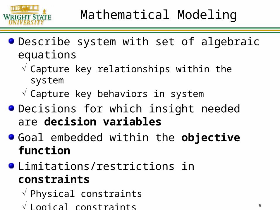
Mathematical Modeling

Describe system with set of algebraic equations Capture key relationships within the system Capture key behaviors in system

Decisions for which insight needed are decision variables

Goal embedded within the objective function

Limitations/restrictions in constraints Physical constraints Logical constraints

9

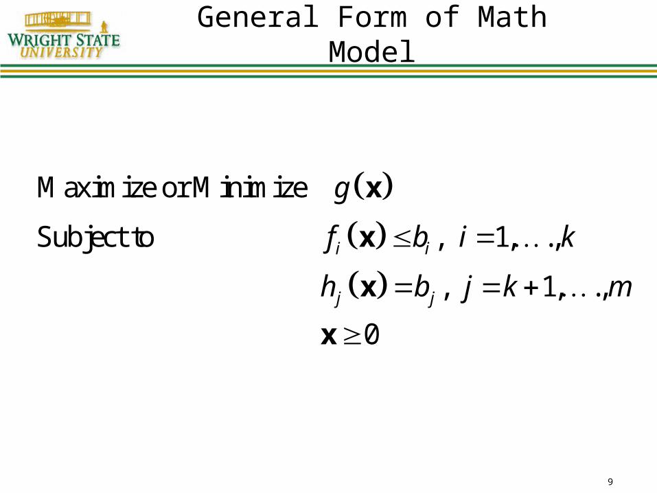
General Form of Math Model

Maximize or Minimize

Subject to , 1, .,

, 1, .,

0

x

x

x

x

i i

j j

g

f b i k

h b j k m

10

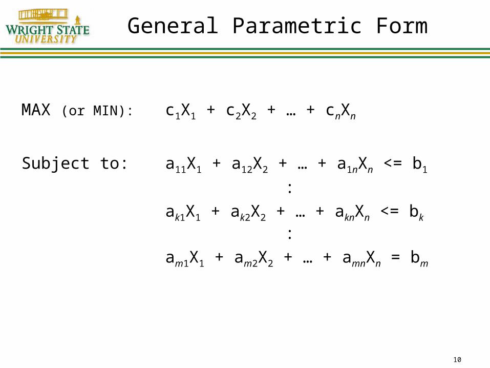
General Parametric Form

MAX (or MIN): c1X1 + c2X2 + … + cnXn

Subject to: a11X1 + a12X2 + … + a1nXn <= b1

:

ak1X1 + ak2X2 + … + aknXn <= bk :

am1X1 + am2X2 + … + amnXn = bm

11

A Simple Example

Blue Ridge Hot Tubs produces two types of hot tubs: Aqua-Spas & Hydro-Luxes.

There are 200 pumps, 1566 hours of labor, and 2880 feet of tubing available.

How many of each type should be produced to maximize profits?

Aqua-Spa Hydro-LuxPumps 1 1Labor 9 hours 6 hoursTubing 12 feet 16 feetUnit Profit $350 $300

12

Model Formulation Process

1. Understand the problem

2. Identify the decision variables

X1=number of Aqua-Spas to produce

X2=number of Hydro-Luxes to produce

3. State the objective function as a linear combination of the decision variables

MAX: 350X1 + 300X2

13

Model Formulation Process

4. State the constraints as linear combinations of the decision variables

1X1 + 1X2 <= 200} pumps

9X1 + 6X2 <= 1566 } labor

12X1 + 16X2 <= 2880 } tubing

5. Identify any upper or lower bounds on the decision variables

X1 >= 0

X2 >= 0

14

Model Formulation Process

MAX: (Objective function)350X1 + 300X2

S.T.: (Constraint set)1X1 + 1X2 <= 200

9X1 + 6X2 <= 1566

12X1 + 16X2 <= 2880

Non-negativityX1 >= 0

X2 >= 0

15

Formulation in Excel Solver

Objective Function$0.00

Decision Variables

X1 0X2 0

Constraint SetPumps 0 <= 200Labor 0 <= 1566Tubing 0 <= 2880

16

2nd Simple Example Model

Objective: Determine production mix that maximizes the profit under the raw material constraint and other production requirements (detailed next).

Maximize 50D + 30C + 6 MSubject to 7D + 3C + 1.5M < 2000 (raw steel)

D > 100 (contract ) C < 500 (cushions

available)D, C, M > 0 (Non-negativity)D and C are integers

17

What We are Looking For

Want to find the best solution

Solution must satisfy each of the constraints

Constraints must be satisfied simultaneously

Common area satisfying all the constraints is called the “feasible region”

ANY point in the feasible region is a possible solution to the problem

What we want is that feasible solution that provides the largest value of the objective function (the “optimal solution”)

18

Feasible Region of an LP

Profit =$4360

500

700

1000

500

X2

X1

19

Linear Programming

Assumptions of the linear programming model The parameter values are known with certainty. The objective function and constraints exhibit constant returns to scale. There are no interactions between the decision variables (the additivity assumption). The Continuity assumption: Variables can take on any value within a given feasible

range.

20

How Do We Solve an LP?

“Solving an LP” = “Finding the best solution possible” = “Finding the optimal solution”

In ISE 470, you will learn the “Simplex Method” of “solving an LP” Uses ideas from “matrix algebra” (i.e. pay attention in

MTH 235) Can be performed by hand using matrix operations

(“pivots”)

The simplex algorithm is available in many forms in software Excel “Solver” Tool Many commercial solver packages (CPLEX, XPRESS,

etc)

21

Integer Programming

Many real life problems call for at least one integer decision variable.

There are three types of Integer models: Pure integer (AILP) Mixed integer (MILP) Binary (BILP) (zero-one variables, on-off)

Unfortunately, these get quite hard to solve Real-world problems can have hundreds or thousands of variables

and constraints Some problems are “theoretically hard”, even when they seem to

have small numbers of elements

Real benefit of these types of models is that we can use binary variables to represent a host of logical conditions within the mathematical formulation

22

Y1 + Y2 + Y3 + Y4 + Y5 + Y6 > 3

1. Three of six projects must be selected.

2. No more than three of six projects can be selected.

Y1 + Y2 + Y3 + Y4 + Y5 + Y6 < 3

Logical Contraints (1)

1 if job is selected

0 otherwise

i

iY

23

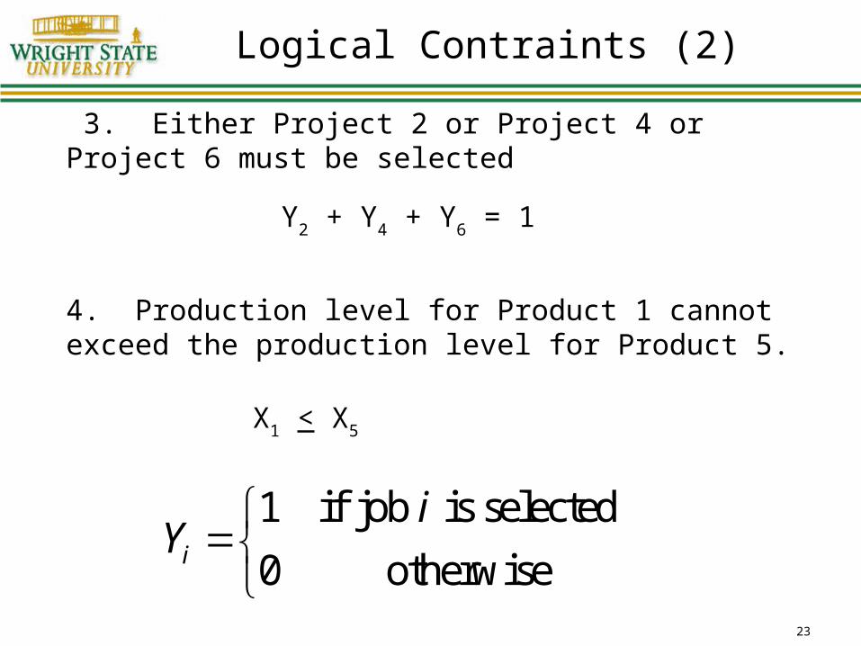
Y2 + Y4 + Y6 = 1

 3. Either Project 2 or Project 4 or Project 6 must be selected

4. Production level for Product 1 cannot exceed the production level for Product 5.

X1 < X5

Logical Contraints (2)

1 if job is selected

0 otherwise

i

iY

24

X4 < MY4

X4 > 120Y4

5. If Product 4 is produced, then at least 120 units of Product 4 must be produced.

6. Four projects are numbered in ascending order. If any project selected, all lower numbered projects must also be selected.

Y2 < Y1

Y3 < Y2

Y4 < Y3

Logical Constraint (3)

25

Y3 < Y4 + Y5

7. If Project 3 selected, either Project 4 or Project 5 must be selected.

8. If Product 6 produced, production must be 50 or 100 units.

X6 = 50Y61 + 100Y62

Y61 + Y62 < 1

Logical Constraint (4)

26

Basic Solution Methods

Linear models – Simplex algorithm Fast in practice Lots of good sensitivity analysis information

Integer models – Branch and bound Can take very long time No sensitivity information Can be sped up with specific knowledge

Nonlinear models Variety of solution methods, usually based on the

“derivative” of the objective function Use “Hill Climbing” and other methods

27

Applications of Mathematical Optimization

Budgeting, capital budgeting

Resource allocation, how much to make

How much to make, how much to contract

Assignment of personnel to jobs Any other kind of assignment application

Funding allocation, investment planning

Inventory planning

Facility layout and planning

28

Applications of Mathematical Optimization

Routing Ever use Google Maps? Pick-up and delivery of items

Selection of items for loading onto delivery trucks

Scheduling Jobs onto machines Patients to doctors Doctors to shifts, workers to shifts

Packing problems, cutting problems How to cut patterns from material

And the list goes on and on…

29

Other Related Areas

Non-linear optimization These involve non-linear functions within the formulations Most applicable solution methods are gradient-based local search

procedures

Modern heuristic optimization These involve integer programming models that are particularly

difficult to solve Also involve non-linear models with forms for which the existing

non-linear solution codes have a particularly hard time solving These are essentially search methods with some pretty strange

analogies to nature Genetic Algorithms Ant-Colony Algorithms Simulated Annealing Algorithms

30

Large-Scale Applications

Airline Crew Scheduling Scenario: A late-day storm has canceled many flights

for American Airlines in and out of Chicago O’Hare Airport. Many planes scheduled to come to Chicago and leave Chicago have not made it to their planned destination for the end of the day

Problem: How should we reassign crews and planes to the routes for the next day, to optimize our use of people, aircraft and other resources?

Companies such as American Airlines, IBM, Hewlett-Packard, UPS, FedEx, Toyota have large-scale problems that are well suited to mathematical optimization

Questions?