Policy Research Working Paper 6673

Is Workfare Cost-Effective against Poverty in a Poor Labor-Surplus Economy?

Rinku MurgaiMartin Ravallion

Dominique van de Walle

The World BankSouth Asia RegionEconomic Policy Unit &Development Research GroupHuman Development and Public Services TeamOctober 2013

WPS6673P

ublic

Dis

clos

ure

Aut

horiz

edP

ublic

Dis

clos

ure

Aut

horiz

edP

ublic

Dis

clos

ure

Aut

horiz

edP

ublic

Dis

clos

ure

Aut

horiz

edP

ublic

Dis

clos

ure

Aut

horiz

edP

ublic

Dis

clos

ure

Aut

horiz

edP

ublic

Dis

clos

ure

Aut

horiz

edP

ublic

Dis

clos

ure

Aut

horiz

ed

Produced by the Research Support Team

Abstract

The Policy Research Working Paper Series disseminates the findings of work in progress to encourage the exchange of ideas about development issues. An objective of the series is to get the findings out quickly, even if the presentations are less than fully polished. The papers carry the names of the authors and should be cited accordingly. The findings, interpretations, and conclusions expressed in this paper are entirely those of the authors. They do not necessarily represent the views of the International Bank for Reconstruction and Development/World Bank and its affiliated organizations, or those of the Executive Directors of the World Bank or the governments they represent.

Policy Research Working Paper 6673

Workfare schemes impose work requirements on beneficiaries. This has seemed an attractive idea for self-targeting transfers to poor people. This incentive argument does not imply, however, that workfare is more cost-effective against poverty than even poorly-targeted options, given hidden costs of participation. In particular, even poor workfare participants in a labor-surplus economy can be expected to have some forgone income when they take up such a scheme. A survey-based method is used to assess the cost-effectiveness of India’s Employment Guarantee Scheme in Bihar. Participants are found to have forgone earnings, although these fall well short of market wages on average. Factoring in these

This paper is a product Economic Policy Unit, South Asia Region; and the Human Development and Public Services Team, Development Research Group. It is part of a larger effort by the World Bank to provide open access to its research and make a contribution to development policy discussions around the world. Policy Research Working Papers are also posted on the Web at http://econ.worldbank.org. The authors may be contacted at rmurgai@worldbank.org and dvandewalle@worldbank.org.

hidden costs, the paper finds that for the same budget, workfare has less impact on poverty than either a basic-income scheme (providing the same transfer to all) or uniform transfers based on the government’s below-poverty-line ration cards. For workfare to dominate other options, it would have to work better in practice. Reforms would need to reduce the substantial unmet demand for work, close the gap between stipulated wages and wages received, and ensure that workfare is productive—that the assets created are of value to poor people. Cost-effectiveness would need to be reassessed at the implied higher levels of funding.

Is Workfare Cost-Effective against Poverty in a Poor

Labor-Surplus Economy?

Rinku Murgai, Martin Ravallion and Dominique van de Walle1

Keywords: NREGA, workfare, public works, poverty, wages, forgone income,

India, Bihar

JEL: I32, I38

Address for correspondence: mr1185@georgetown.edu

1 Murgai and van de Walle are with the World Bank and Ravallion is with the Department of Economics, Georgetown University and the NBER. This paper draws on data collected and analysis done for a World Bank project co-managed by Puja Dutta and Rinku Murgai. The authors are grateful to Sunai Consultancy Private Ltd and GfK Mode for support on the field work for this study. The authors are also grateful to the Rural Development Department, Government of Bihar, for providing insights into the challenges and ongoing initiatives in Bihar. Arthur Alik Lagrange and Maria Mini Jos provided very able research assistance. Useful comments were received from seminar participants at the Indian Statistical Institute, the Paris School of Economics, the Australian National University, Georgetown University and the World Bank. These are the views of the authors and do not necessarily represent those of their employers, including the World Bank or of any of its member countries.

2

1. Introduction

Workfare schemes impose work requirements on welfare recipients. The policy

arguments for doing so have rarely been based on the value of the outputs from that work. Rather

they have been that workfare deals with the problem of targeting when informational and

administrative constraints preclude optimal income taxes/transfers. By only attracting those in

genuine need, and encouraging a return to the regular workforce when help is no longer needed,

workfare incentivizes behaviors that solve the problem of knowing who is genuinely “poor” and

who is not (Besley and Coate, 1992).

In probably the most famous example of the use of this “self-targeted” feature of

workfare, welfare recipients in pre-modern Europe were often incarcerated in “workhouses”

where they were obliged to work for their upkeep and their “bad behaviors” could be controlled.

From the outset, the idea was that only the poorest would be willing to be so confined.

Workhouses were thus seen as a cost-effective means of poverty relief (Thane, 2000, p.115).

Reforms to England’s Poor Laws in 1834 famously used workhouses to ensure better targeting,

and this appears to be the main reason that public spending on relief fell from 2.5% of national

income around 1830 to 1% in 1840 (Lindert, 2013, Figure 1).

But is workfare really cost effective? There is evidence that workfare is indeed self-

targeted. For example, in the workfare scheme in India studied in this paper, the mean

participation rate falls steadily from 35% of the population for the poorest few wealth percentiles

to nearly zero for the richest (Dutta et al., 2013). Without any explicit effort at targeting the poor,

participation favors poor families. However, even excellent targeting matters little if the net gains

to workfare participants are small. This could be expected if the scheme offers market wage rates

in a competitive, fully-employed, economy. However, workfare tends to be advocated in places,

or at times, with high unemployment, such as during recessions, famines or lean agricultural

seasons. Advocates often assume (explicitly or implicitly) that workers would be idle in the

absence of the scheme, and conclude that the net gain is the workfare wage.

Is that assumption plausible? The famous Lewis (1954) model of economic development

assumes that labor can be absorbed from peasant farming into the modern sector with little or no

loss of rural output. However, as Rosenzweig (1989) points out, this requires either zero marginal

product of rural farm-labor or that, with one less worker on the family farm, other family

members make up the difference by working harder. One can question the plausibility of both

3

conditions. More generally, there is also a private rural labor market, with some probability of

finding work during any period of workfare participation.

The forgone income of workfare participants is unlikely to be negligible even with

reasonably high unemployment overall. Self-targeting is essentially ensured when the private

opportunity cost of participation is lower for poorer people. But it is unlikely to be zero for all.

The magnitudes of these hidden costs clearly matter to the policy choice. In an influential policy

report, World Bank (1986) argued that workfare schemes are unlikely to be cost effective against

poverty given the private opportunity costs of labor. No evidence was presented.

We still know very little about the forgone earnings of workfare participants. Standard

evaluation methods rely on comparing means between those treated and a selected comparison

group of non-participants. Various methods are used to assess impacts under maintained

identifying assumptions, including econometric models of time allocation and matching

estimators. Estimates of mean forgone income have varied from 25% of workfare earnings (in

Maharashtra, India) to 50% (Argentina).2

However, a potentially large amount of economically relevant, individual-specific

information on forgone opportunities is left unobserved by these methods. And this information

is clearly known by those deciding whether to participate. This gives rise to what Heckman et al.

(2006) term “essential heterogeneity” (also known as “correlated random coefficients” in a

regression model), which they show can confound inferences about even the overall mean impact

from standard econometric estimators (including those using randomized assignment as an

instrumental variable). Such heterogeneity has long been a concern in the evaluation literature.3

The problem stems from the evaluator’s lack of information about forgone opportunities.

There is an alternative non-parametric method of addressing the heterogeneity problem by

simply posing counterfactual questions to participants. Then we do not need to make any of the

standard assumptions of econometric estimators, notably the assumption that the regression error

term has mean zero, conditional on either treatment status or some correlate (the instrumental

variable) of that status. This method has the advantage that we can estimate mean impacts,

2 From Datt and Ravallion (1994) and Jalan and Ravallion (2003) respectively. The result for Argentina was confirmed (using different methods) by Ravallion et al. (2005). Other evaluative studies of workfare include Ravi and Engler (2013), Liu and Deininger (2013), Imbert and Papp (2012), Berg et al. (2012) and Zimmerman (2012). 3 Early discussions include Heckman and Robb (1985) and Björklund (1987).

4

including on poverty measures, non-parametrically, assuming nothing more than classical

measurement errors in survey responses.

It may be noticed that this method is similar in some respects to expectations surveys, in

which respondents are asked for their point expectation for some event or variable at some point

in the future, which cannot be directly observed at present. Here we are also asking about an

unobserved state—the outcome in the absence of the workfare scheme. The difference is that we

are asking about a concurrent counterfactual state rather than a future state. Essentially each

sampled participant is asked for their expectation of employment and earnings if they did not

have the workfare opportunity at the time. While we acknowledge that counterfactual survey

questions can be difficult, we found that with care in design, response rates were high and (as we

will show) the answers make sense.

We apply this method to a workfare scheme in the Indian state of Bihar. This is one of the

poorest states of India (the poorest by some measures), with 55% of its rural population of 90

million living below the official poverty line in 2009/10.4 At the same time, the rural

unemployment rate of 18% (16% for men and 32% for women) is twice the national average

(Ministry of Labour and Employment, 2010). The rate of under-employment (workers whose

normal status is employed but work less than they want) is likely to be even higher. This is the

type of poor labor-surplus economy in which workfare schemes have been seen to have much

promise for fighting poverty. With that aim in mind, a large national workfare scheme was

introduced in 2005, promising to give up to 100 days of unskilled manual work per year to any

rural household that wants it.

The paper asks whether the pure workfare aspect of this ambitious scheme is sufficiently

pro-poor to justify it as an efficient means of transferring money to poor people. Could it be that

the information constraints are so severe and the unemployment rate so high that the self-

targeting mechanism using work requirements tilts the balance in favor of workfare even if the

work produces nothing of value? Or are the latent forgone incomes too large even in this poor

labor-surplus economy?

An important issue in addressing these questions is the choice of the counterfactual. It

would hardly be surprising that one can reduce poverty by spending public money on a large

4 This is based on official Planning Commission poverty lines for 2009/10. The state has had one of the lowest long-run trend rates of poverty reduction in India; indeed, there was virtually no long-run trend over 1960-2000 (Datt and Ravallion, 2002).

5

workfare program under ideal conditions (largely financed by taxation on the non-poor).

Arguably the more interesting question is whether a greater impact is possible with some feasible

alternative allocation of the same public resources. An obvious counterfactual is a basic-income

scheme (BIS).5 This provides a fixed cash transfer to every person, whether poor or not. There is

no explicit effort at targeting and no incentive effects of the transfers since there is no action that

anyone can take to change their transfer receipts.6 The administrative cost would probably be

low, though not zero given that some form of personal registration system would be needed to

avoid “double dipping” and to ensure that larger households receive proportionately more. A

basic income scheme could be costly (depending on the benefit level and method of financing)

although there may well be ample scope for financing by cutting current subsidies favoring the

non-poor, as Bardhan (2011) argues is the case for India. However, a basic-income scheme would

require a new public delivery mechanism. An alternative counterfactual of interest because of its

near-term feasibility is to use existing targeting instruments, however imperfect, as the delivery

mechanism for budget-neutral transfers. We provide impact estimates relative to both a BIS and

using India’s existing delivery mechanism for targeted food rations.

The following section discusses the program under study, while Section 3 describes our

data and estimation methods. Section 4 examines what we learn from the survey data about the

wages received by workfare participants. Section 5 turns to our findings on forgone incomes.

Combining these elements, Section 6 provides our estimates of the poverty impacts relative to

budget-neutral alternatives. Section 7 concludes.

2. The program

India has had a long history of workfare schemes. The essential idea was embodied in the

Famine Codes introduced in British India around 1880, and such schemes have continued to play

an important role to this day in the sub-continent. An important sub-class of workfare schemes

has aimed to guarantee employment to anyone who wants it at a pre-determined (typically low)

wage rate. Such Employment Guarantee Schemes (EGSs) have been popular in South Asia,

5 This has been called many things including a “poll transfer,” “guaranteed income,” “citizenship income” and an “unmodified social dividend.” BISs have been proposed by (amongst others) Meade (1972), Atkinson and Sutherland (1989), Ravallion and Datt (1996), Raventós (2007) and Bardhan (2011). 6 While a basic income scheme is unlikely to alter incentives to work (say), a complete assessment of the implications for efficiency (and equity) must take account of the methods of financing the poll transfer, and once one allows for financing, the incentive and information issues re-emerge.

6

notably (though not only) in India where the Maharashtra EGS started in 1973 and was long

considered a model (Drèze, 1990; Ravallion, 1991). In 2005, India’s central government

implemented a national version, now called the Mahatma Gandhi National Rural Employment

Guarantee Scheme (MGNREGS). This promises 100 days of work per year per rural household

to those willing to do unskilled manual labor at the statutory minimum wage notified for the

program. The work requirement is (more or less explicitly) seen as a means of assuring that the

program is reaching India’s poor. The available evidence does suggest that the scheme is quite

well targeted to poor rural households; see Alik-Lagrange and Ravallion (2012) for India as a

whole and Dutta et al. (2013) for Bihar.

MGNREGS explicitly aims to reduce rural poverty and the promise has been great.

Indeed, advocates have claimed that it could largely eliminate poverty in rural India. For

example, Drèze (2004) claimed that the scheme “...would enable most poor households in rural

India to cross the poverty line.” That might seem a tall order, but there can be no denying that this

is an ambitious and well-intentioned effort to fight poverty in India and that, in principle, it has

huge promise. The sheer scale is impressive; according to the administrative data, over 50 million

households participated in MGNREGS in 2009/10.7 The scheme is nation-wide. Here we focus

on one state, Bihar, as discussed in the introduction. We refer to MGNREGS in Bihar as BREGS.

The first and most direct way this scheme tries to reduce poverty is by providing extra

employment on demand in rural areas and in a way that is self-targeted to poor people.

Intuitively, it is easy to imagine that low-wage manual labor, often under a hot sun, would not be

attractive to anyone who is not in fact poor. However, we already know from the literature and

field observations that there are a number of ways that the potential impact on current poverty of

this scheme might not be realized in practice (Dutta et al., 2013):

• The supply side may be slow to respond to the demand for work on the scheme.

• Workers may be unable to meet productivity norms for earning the minimum wage.

• There may be delays in payment (random or purposive).

• Corruption may be present, whereby local leaders or officials take their cut.8

• There may be exploitation, stemming from the monopsony power of the village leader,

essentially acting as a contractor. 7 See Government of India website for MGNREGS (http:\\nrnic.in). 8 For example, local officials may charge a “fee” for their services, such as providing wages in advance or collecting wages against “ghost workers.”

7

• There may be forgone income, i.e., an opportunity cost to the worker from forgone

economic activity such as similar work in the casual labor market.

Dutta et al. (2012) report all-India survey results indicating substantial unmet demand for

work on MGNREGS. This is based on the National Sample Survey (NSS) for 2009/10. With the

survey instrument used in this paper (designed specifically for this purpose), Dutta et al. (2013)

also find evidence of considerable un-met demand for work on BREGS. Of those demanding

work on the scheme, only one-third got that work.

A second way in which the scheme can potentially reduce poverty is by creating assets of

value to poor people (either directly or indirectly, such as through private employment effects).

This aspect of MGNREGS has had less attention than the direct employment gains to

participants. A widely heard characterization says that the assets are mostly worthless, but this is

clearly an exaggeration. Verma (2011) reports field work assessing the returns to 140 water-

based projects under MGNREGS. The results suggest that some MGNREGS projects do bring

lasting positive benefits beyond the direct employment. However, the sample was purposively

selected in favor of the “best-performing” projects and so cannot be used to generalize about the

portfolio of projects. There have been many anecdotal observations about the lack of local

capabilities for devising and maintaining projects and a lack of interest among local engineers.9

There have also been anecdotal observations that any durable asset creation on the scheme has

often favored local landowners and politicians, rather than poor households directly, who are

typically landless.

MGNREGS is not, of course, the only anti-poverty program in India. The country also has

a system of subsidized food rations based on an assignment of “Below Poverty Line” (BPL) cards

done by state governments and delivered through local outlets with wide coverage. The BPL

ration card is intended to define the poverty status of households for determining entitlements to

food subsidies and other government programs. There have been many claims that BPL cards are

not as well targeted to the poor as they could be.10 Here we take the existing assignment of cards

in our survey data as given and use it to construct an alternative counterfactual for assessing the

9 See, for example, the comments in Verma (2011), Mann and Pande (2012) and Zimmerman (2012). 10 For example, Besley et al. (2012) find that being a local politician makes it more likely that someone will have a BPL card after controlling for wealth indicators, including landlessness. At the time of writing the BPL card system is under review by the Government of India. Food rations will no longer be restricted to only those with the BPL card; setting criteria for targeting (albeit at higher coverage levels) has been left to the decision of individual State governments.

8

cost-effectiveness of workfare, namely an allocation of the same budget but assigned instead as

transfers in cash or in kind to those holding BPL cards.

3. Data and methods

For the purpose of this study, we collected two rounds of data in a household panel

structure from 150 villages spread across rural Bihar. The first round (R1) was implemented

between May and July of 2009 and the second (R2) during the same months one year later. These

periods were chosen for being lean periods for agricultural work, and were thus expected to be

peak periods for BREGS. Both rounds included questions with recall over the previous 12

months. The year preceding the first survey period witnessed severe floods during the monsoon

(July-August of 2008) in some districts falling in the catchment area of the Kosi River. In

contrast, rainfall was scanty during the 2009 monsoons and drought was declared in many

districts during the second survey period.

A two-stage sampling design was followed, based on the 2001 Census list of villages. In

the first stage, 150 villages were randomly selected from two strata, classified by high and low

BREGS coverage based on administrative data for 2008/9. In the second stage, 20 households per

village were randomly selected, drawing from three strata based on an initial listing of all village

members and a few selected attributes. This stratified approach ensured that the sample included

both scheme participants and households with likely participants. We have used the appropriate

sample weights to reflect the sampling design.

The surveys collected information on a range of household level characteristics including

demographics, socio-economic status (including asset ownership and consumption), employment

and wages, political participation and social networks, as well as information on BREGS

participation and process-related issues. Two household members, one male and one female,

were interviewed about their participation in BREGS, experience of BREGS at the most recent

worksite and knowledge and perceptions of the program, the village labor market and the role of

women. In addition, in each village, key informants were interviewed about physical and social

infrastructure in the village, and access to government programs.

In total, 3,000 households and approximately 5,000 individuals were interviewed in both

rounds. The balanced panel comprises 2,728 households and 3,749 individuals. The overall

attrition rate for households between the two rounds is 8% and is not concentrated in any

9

particular stratum. There were relatively few refusals; two-thirds of the attrition was because a

household was away temporarily when the survey team visited the village.

We also initiated qualitative research in purposively selected villages in six districts in

north and south Bihar (Gaya, Khaimur, Kishanganj, Muzaffarpur, Purnea and Saharsa) during

February and August 2009.11 The results of this qualitative work will be used in interpreting

some of our quantitative findings.

Our method of measuring forgone incomes relies on asking participants themselves what

they think they would have done in the absence of the program.12 If they said that they would

have worked, we asked them how many days and at what wage. The specific questions (in the

local dialect) were fine-tuned in the piloting stage. As noted in the introduction, our method has

the advantage that we obtain individual-specific impacts, incorporating idiosyncratic information

on the available opportunities—information that would be unlikely to be available as data in an

observational study. We are thus able to implement quite fine distributional analysis, as required

for assessing impacts on poverty.

Counterfactual questions are not always easy for respondents. However, this did not

appear to be a problem in our case. With appropriate training for interviewers, quite high

response rates were obtained. The overall response rates to our questions on forgone income were

92% in the first round of our survey, up to 98% in the second round.13

In common with most other methods of impact evaluation using micro data, there may be

general equilibrium effects that this method cannot hope to identify. In the present context, two

different survey respondents may have in mind the same forgone work opportunity, such that

aggregate forgone income will be lower than the sum of the individual reports. We will test the

sensitivity of our results to the possibility that our methodology has led us to over-estimate

forgone earnings.

Certain protocols were established for cleaning and analyzing these data:

11 The qualitative results are reported in Development Alternatives (2009), Indian Grameen Services (2009) and Sunai (2009). Dutta et al. (2013) provide summaries of the findings and their implications. 12 Jha et al. (2012) also asked survey respondents working on MGNREGS whether they thought any other work was available. They did not, however, ask for forgone incomes, but instead used prevailing wage rates for the imputation. 13 Exploiting our survey design, we can also confirm the reliability of reported forgone incomes for the main relevant activity, namely casual work; see Dutta et al. (2013).

10

• For housework or own-enterprise (typically own-farm) work, forgone income was

assumed to be zero, on the plausible assumption that such work can be readily re-

allocated over time to ensure little or no forgone income.

• Forgone work and incomes were asked for each spell of BREGS work, for each

individual. The gender-specific median was then used as the household value.

• Missing values of forgone income were replaced with the median for the household’s

stratum in the village or the village median (across all strata) if it was still missing.

• About 10% of respondents reported forgone earnings greater than their earnings from

public works. This is implausible, and most likely reflects a misunderstanding of the

survey question. We assumed that this was an error and so we truncated the data such that

forgone income in any period cannot exceed earnings from public works.

In estimating poverty measures, we use a comprehensive consumption aggregate (using a

survey module based on the NSS Employment-Unemployment Schedule). The poverty line is the

median per capita consumption level in R1 and we update this over time using the Consumer

Price Index for Agricultural Laborers to get the R2 line. This gives poverty lines of Rs. 6,988 per

person per year in R1 and Rs. 7,836 in R2. However, recognizing that any poverty line is bound

to be somewhat arbitrary, we also provide estimates of the poverty impacts over a wide range of

potential lines.

In setting the cost of the scheme for the counterfactual analysis, we include all public

expenditures attributed to BREGS in the central administrative data. These include materials and

supervision as well as BREGS wages; these non-wage costs represented 36% and 39% of total

spending on the program in Bihar in R1 and R2, respectively (Dutta et al., 2013). The precise

budgets we use are Rs. 858.42 per household in R1 and Rs.1,194.92 per household in R2.14

The calculation of counterfactual poverty measures is then a simple accounting exercise.

The actual (observed) post-BREGS poverty measure is based on the observed distribution of

consumption per person y = (y1,….,yn) (where yi is consumption per person for household i). The

counterfactual in the absence of BREGS is based instead on the distribution y – w + f where w is

the n-vector of actual wages received from BREGS and f is the n-vector of forgone incomes due

14 The administrative data indicate total expenditures of Rs 13,058 million in FY 2008-09 and Rs 18,177 million for FY 2009-10 (Dutta et al., 2013, Chapter 1). These were divided by our count of 152 million households in rural Bihar, as implied by our survey weights. Recent Census projections gave slightly higher counts but it is better to use our survey-based numbers for internal consistency.

11

to taking up that work. The difference between the measures based on these two distributions

then gives the impact on poverty. When instead the counterfactual is the basic income scheme,

the poverty measure is based on the distribution y – w + f + c where c is the cost of the scheme

per person (wage plus non-wage costs). (This can be scaled down to allow for leakage.) For the

counterfactual based on the current assignment of ration cards, the relevant distribution is instead

y – w + f + (c/ p)r where r = (r1,….,rn) denotes the assignment of ration cards (ri=1 if i has a BPL

card and ri=0 if not) and p is the proportion of households with a ration card.

4. Wages

There are a number of ways in which BREGS implementation differs from the formal

guidelines, with bearing on the wages received and (hence) poverty impacts. During the survey

period, the notified BREGS wage started at 89 rupees per day, rising to 102 in June 2009, and to

114 in May 2010. Productivity norms are stipulated such that an able-bodied worker can earn

these notified wages. Scheme functionaries are required to ensure that these norms are being met

by measuring the work done at the worksite. Yet, nearly half of the men and women workers

interviewed reported seeing no one measuring work at their most recent worksite. When

measurement was done, among those aware of the process, the majority (83% of the male and

75% of the female workers interviewed) reported equal payments to all workers at the site. When

we asked Mukhiyas (elected village leaders) why workers reported not being paid the stipulated

BREGS wage, they typically responded that workers had not performed to the productivity norms

and hence were not owed the stipulated wage. They also told us that workers often did not

understand this.

Since April 2008, in an effort to promote financial inclusion and transparency in wage

payments, all wages are supposed to be paid through beneficiary bank or post office accounts

rather than as direct cash payments. The practice is unclear, based on our surveys and field work.

Officials report that the majority of wage payments are made through bank or post office

accounts. But workers report that wage payments are more often made in cash at the worksite. In

2010, more than half of the workers interviewed—52% of women and 56% of men—reported

receiving wages in cash from the Mukhiya, the contractor, the mate or another official at the most

recent worksite at which they worked. In R1 the percentages were 78% and 64% for female and

male workers, respectively. Thus, while there is evidence of a decline over time, the share of

12

total workers getting cash at worksites remains high. In some cases this may reflect partial cash

payments to workers by the Mukhiya while funds are being transferred to worker accounts.

The Mukhiya or his/her spouse or close family member often act as money lenders as well

as contractors, making advance payments to workers.15 The reasons given include delays in work

measurement, delays in obtaining post office/bank accounts and delays in the flow of funds to the

worker post office or bank accounts.16 In principle, the scheme should move towards full reliance

on formal accounts rather than cash. But at the time of our survey, practice was still a long way

from that ideal. Weaknesses in the flow of funds or administration of accounts, leading to delays

in payment, create scope for the Mukhiya or other intermediaries to profit by being able to

provide advance cash payments to needy workers.17 Fieldwork for this study indicated that some

local officials also take a cut from the wages due to the worker, possibly in the process of making

advance payments.

There have been qualitative reports from the field of partial payments and long delays in

receiving wages. Our survey provides corroboration. We asked whether BREGS participants had

received wages owed in full. In the surveyed households, 72% of the female participants in R1

and 67% in R2 had been paid in full by the time of our survey, while this was the case for 66%

and 72% of participant men. Women who had not been fully paid were still owed 58% and 75%

of wages on average in R1 and R2, respectively. Unpaid men were still waiting for 64% and

57% of their earned wages. The amount owed is likely to decline as time since participation

increases. Our data confirm that the share of wages received is higher for participants for whom

more time has elapsed since they participated in BREGS. This can be seen in Figure 1, plotting

the share of wages owed that were actually received by months since the work was completed for

those who have not received their full wages. The mean share of wages paid rises with time up to

six months, then stabilizes (R1) or falls (R2). However, even at its peak, the share of wages

received among those receiving less than they felt they were due is no more than 50%.

There has been hope among advocates that the scheme would reduce the exploitation of

rural workers in local labor markets stemming from the labor-market power of large farmers or

15 As in other states, one third of elected positions are reserved for women in Bihar. Thus, elected Mukhiyas are sometimes female. However, once the election is over, a male surrogate, frequently a husband, often plays an active role in the job. When we refer to the Mukhiya we mean either the elected or surrogate one. 16 Also see the discussion in Khera (2011). 17 This is not confined to Bihar; Vanaik (2009) reports the same practice in Rajasthan—thought to be amongst the better performing states in implementing MGNREGS.

13

contractors. This might well have been a tall order given that the local leaders in charge of

implementing the scheme often overlap with the set of people who have been employers in the

past. For example, the Mukhiya, acting as a contractor directly or via a close ally, can maintain

similarly exploitative relations in implementing the scheme. The scheme officially bans

contractors, but they are common, with half or more of the responding workers reporting that

contractors were present at worksites.

4.1 Wages received by households

The BREGS survey obtains wages from two sources. Block 23 of the household

questionnaire asks about earnings and days of work in the week preceding the survey for each

adult household member.18 It differentiates between public works (PW) and other casual wage

work, but does not differentiate between BREGS and other PW employment.19 Wage earnings

include cash payments and the value of in-kind payments. In addition, for each work activity, the

questionnaire records information separately on wages that were owed and wages that had

already been received. We expect one-week recall to be excellent but the data have the

disadvantage that they provide relatively few observations. Since the survey was fielded in the

May-July months, wage information from this Block pertains only to these months.

The second source of information about wages is from the individual level questionnaire

(Block 1) which asked (up to) one male and female adult in each household about their

involvement in public works specifically, including type (whether BREGS or other), days

worked, wages owed, and wages received separately for each episode of public works

employment over the last year. These are the data that we have already made reference to above

with respect to delays in wages paid. In addition to providing details specifically about BREGS,

this source gives many more observations than Block 23. The drawback is that there may be mis-

measurement due to the long recall period and that this does not give wages for non-PW work.20

Given the different pros and cons of each source, we make use of both.

18 Block 23 is adapted from the standard weekly module in the NSS Employment-Unemployment (Schedule 10) surveys. 19 Other public works employment could include BREGS, road building projects or other public works schemes run by the state Government. 20 To reduce sensitivity to measurement errors we treat the (very few) recorded wages over 200 Rupees per day or under 10 Rupees from both sources as missing values.

14

Table 1 reports summary statistics on casual wages for the week prior to the survey. In R1

(2009), median PW wages were nearly 30% higher than the casual wage. Wages are higher for

men than for women in both segments of the labor market, but for women, PW pays much better

than the private sector. Between 2009 and 2010, average PW wages maintained value in real

terms (increasing by 14.6% in nominal terms, compared to a 12% rate of inflation),21 but the gap

between public works and labor market wages narrowed as mean casual wages rose by 21%, and

median casual wages rose by 43%. Women, however, still earned significantly higher wages

under BREGS in R2 than in the casual labor market (t=3.91 in R1 and t=4.85 in R2).

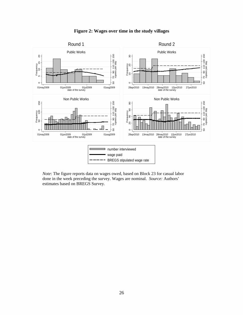
Figure 2 and Table 2 take a closer look at wages for casual labor in relation to the

stipulated BREGS wage, and their evolution over time. It can be seen that wages owed, as

reported by participants on the scheme, are lower than the stipulated BREGS wage rate (top

panels of Figure 2). Summary statistics and tests reported in Table 2 show that on average,

workers received Rs. 10 less per day than the stipulated wage, for much of the recall period.

Note that this gap is not due to payment delays, as the wages summarized are total wages owed to

the individual, not the amount actually received by the time of the survey interview.

Turning to the second source of data on wages on BREGS from our survey, Figure 3 plots

the mean wage rate by month for both men and women based on Block 1. The figure also gives

total days of work and identifies the survey periods. There is a marked seasonality in days of

employment. As before, we see a persistent gap between the stipulated BREGS wage rate and the

wage actually reported. The absolute gap is roughly unchanged over time. There is some sign of

convergence in male and female wages, but this is possibly deceptive, given that there were very

few observations in the early months when the female wage was lower. The longer recall periods

required by this source of wage data also raise doubts about the early data points.

A third source of wage data is the NSS for 2009/10. Table 3 reports mean and median

wage rates, spanning the period between R1 and R2 of the BREGS survey. Here too we see an

increase in agricultural wages, notably between sub-rounds 2 and 3, corresponding to the last

quarter of 2009 and first quarter of 2010. BREGS activity picks up in the first quarter of the year,

so this agricultural wage increase does coincide with BREGS. However, also note that there was

an even steeper increase in manual non-agricultural wages over the year.

21 The inflation rate is based on the consumer price index for agricultural laborers in the state.

15

How do the wages compare? Figure 4 provides the density functions for daily casual work

wages (in the week preceding the survey) for public works (PW) and three comparators: (i) the

non-PW wages for BREGS participants; (ii) the non-PW wages for the excess demanders (those

who wanted but did not get work on BREGS); and (iii) the non-PW wages of all others. Wage

rates were calculated by taking total wage earnings by type of work in the week prior to the

interview and dividing by the total number of days of such work reported.

Two points are worth noting. First, as already discussed, PW wages are higher than other

casual wages earned by BREGS participants, for both men and women. We can reject the null

hypothesis of equality between the PW wage and the non-PW distributions for both men and

women in R1 (probability less than 0.0005 in both cases). This is true for other comparator

groups as well: the people who said they wanted work on BREGS but did not get it (the excess

demanders) were typically earning less than those working on PW.

Second, the difference between BREGS wages and other casual wages does not appear to

be due to different abilities of the workers. It could be possible that piece work schedules such as

used by BREGS reward physically stronger workers. However, this does not appear to be the

explanation, since we also see that BREGS participants were earning significantly less in non-

PW work than in PW. In fact there is no statistically significant difference between the wage

distributions of the three comparators for either women or men.22

And there is essentially no difference between the wage distribution for the “excess

demanders” and the non-PW wage distribution of those who also do PW. Those who get the jobs

on PW are essentially drawn from the same wage distribution as those who do not get that work,

but want it. This is again suggestive of unmet demand for work stemming from some form of

rationing in the assignment of jobs, as documented by Dutta et al. (2012).

4.2 Impact of BREGS on wages

If BREGS provided an un-conditional guarantee of work to anyone who wanted it at a

wage at or above the wage for alternative work, then the BREGS wage rate would become

binding on the casual (farm and non-farm) labor market. Nobody would be willing to work at less

22 The Kolmogorov-Smirnov (KS) test does not reject the null hypothesis that the distributions are identical in the three binary comparisons between the three comparison wage distributions for either men or women.

16

than the BREGS wage rate. There may be lags in the adjustment process, but we would expect to

see casual wages catching up to BREGS wages.

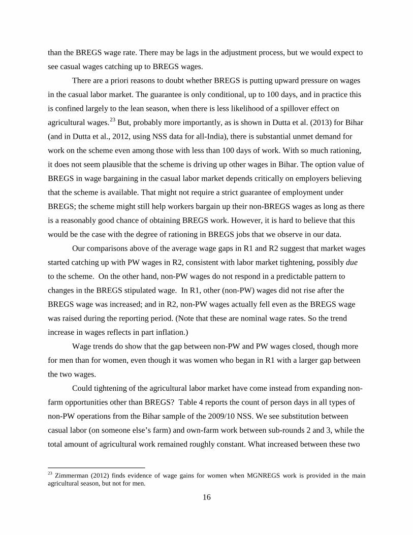
There are a priori reasons to doubt whether BREGS is putting upward pressure on wages

in the casual labor market. The guarantee is only conditional, up to 100 days, and in practice this

is confined largely to the lean season, when there is less likelihood of a spillover effect on

agricultural wages.23 But, probably more importantly, as is shown in Dutta et al. (2013) for Bihar

(and in Dutta et al., 2012, using NSS data for all-India), there is substantial unmet demand for

work on the scheme even among those with less than 100 days of work. With so much rationing,

it does not seem plausible that the scheme is driving up other wages in Bihar. The option value of

BREGS in wage bargaining in the casual labor market depends critically on employers believing

that the scheme is available. That might not require a strict guarantee of employment under

BREGS; the scheme might still help workers bargain up their non-BREGS wages as long as there

is a reasonably good chance of obtaining BREGS work. However, it is hard to believe that this

would be the case with the degree of rationing in BREGS jobs that we observe in our data.

Our comparisons above of the average wage gaps in R1 and R2 suggest that market wages

started catching up with PW wages in R2, consistent with labor market tightening, possibly due

to the scheme. On the other hand, non-PW wages do not respond in a predictable pattern to

changes in the BREGS stipulated wage. In R1, other (non-PW) wages did not rise after the

BREGS wage was increased; and in R2, non-PW wages actually fell even as the BREGS wage

was raised during the reporting period. (Note that these are nominal wage rates. So the trend

increase in wages reflects in part inflation.)

Wage trends do show that the gap between non-PW and PW wages closed, though more

for men than for women, even though it was women who began in R1 with a larger gap between

the two wages.

Could tightening of the agricultural labor market have come instead from expanding non-

farm opportunities other than BREGS? Table 4 reports the count of person days in all types of

non-PW operations from the Bihar sample of the 2009/10 NSS. We see substitution between

casual labor (on someone else’s farm) and own-farm work between sub-rounds 2 and 3, while the

total amount of agricultural work remained roughly constant. What increased between these two

23 Zimmerman (2012) finds evidence of wage gains for women when MGNREGS work is provided in the main agricultural season, but not for men.

17

sub-rounds was the amount of manual non-farm work. The rising availability of this work could

well be driving up the agricultural wage rate in this period, rather than BREGS.

Respondent perceptions that improvements in both wages and employment opportunities

are unconnected to BREGS (see Dutta et al., 2013) are also consistent with this reading of the

evidence. Workers can be expected to know whether BREGS is enhancing their bargaining

power in the labor market, but they do not think so overall. Recall that for women the gap

between public and non-public works wages was much less affected than that for men over the

period. The fact that men are generally more likely than women to be engaged in casual off-farm

work gives added weight to our interpretation.

Note that there may well be larger impacts on wages in states of India where there is less

rationing. As Dutta et al. (2012) show, there is far more rationing in some states than in others.

The scheme may well be having larger impacts on private sector wages in states with less

rationing. Indeed, Imbert and Papp (2012) present evidence that in states with more effective

implementation, the scheme has had more impact on casual wages.

4.3 A fuzzy wage floor?

If the scheme guaranteed employment at the stipulated wage rate, it would provide a

binding wage floor across all casual work, including in the private sector. Given the extensive

rationing we have documented, this is not what we expect to find. But how close does it come in

practice to providing even a wage floor for PW labor?

To answer this question, we need to examine the distribution of the wage rates received

relative to the stipulated BREGS wages. To see how the wages reported in the BREGS survey

compare to the stipulated wages for MGNREGS in Bihar, we divide the survey wage rate (for the

week before the interview) by the stipulated wage rate in Bihar for that week. In R1 the

(unweighted) mean of this ratio is 0.88 (st.dev.= 0.16), and in R2 the mean is 0.86 (s.d.=0.21).

The corresponding medians are 0.91 and 0.88.

It is evident from the medians that about half the workers on PW earned less than 90% of

the stipulated wage rate. Figure 5 shows the full distributions of this ratio; in each case we give

both the densities and the cumulative distribution, to see more clearly how many workers were

earning less than the stipulated wage rate. For R1 we see that about the same percentage of PW

workers were earning less than the stipulated wage rate as for non-PW workers. For R2, we find a

18

slightly higher proportion of workers on PW earn less than the stipulated wage rate than of

workers on non-PW work. However, this is deceptive, given the greater compression of PW

wages. This is clear if we calculate the proportion of workers earning less than 75% of the

stipulated wage rate. For example, in R1, only 14% of PW workers earned less than 75% of the

stipulated wage rate, as compared to 46% of non-PW workers. In R2 the corresponding

proportions were 21% and 45%. It appears that BREGS is able to provide participants a “fuzzy

wage floor” that is not available for other casual work.

Figure 6 examines whether there is a difference in the wage floor for men versus women.

We use data from Block 1 in the individual questionnaire, which is based on one-year recall and

therefore has more observations for a gender-wise disaggregation. In means and medians, the

ratio of the BREGS wage rate to the stipulated wage rate was similar for both men and women, in

both rounds.24 However, the gap widens at lower proportions of the stipulated wage rate (as is

evident from the cumulative distributions in Figure 6).

The proportion of women earning considerably less than the stipulated wage rate is higher

than for men in both rounds. In R1, 19% of women were earning less than 75% of the stipulated

wage rate, as compared to 13% of men. The gap narrowed slightly in R2, with 15% of women

earning less than 75% of the stipulated wage rate, versus 11% of men. It is clear that BREGS is

even less effective in providing a wage floor for women than for men.

5. Forgone earnings

Recall that to measure forgone earnings we asked counterfactual questions of BREGS

participants in our surveys, to obtain their assessment of how many days they would have

otherwise worked and what they think they would have earned if they had not been doing the

BREGS work during that period (Section 2).

We found that forgone opportunities varied considerably across workers. Table 5

summarizes the types of activities that BREGS-participants identified as being displaced by their

BREGS work. For men, about 14% in R2 (less in R1) said they would have migrated if not for

BREGS; this was only true of 1% of women in R2. Casual work in agriculture was identified as

the forgone work opportunity for about 22% of men and 25% of women in R1. Casual non-farm 24 The mean ratio was 90% for men in both rounds; for women the means are 87% and 89% in R1 and R2, respectively. Medians were similar, with half the workers (of both genders) earning less than 91% of the stipulated wage rate in R1 and 96% in R2.

19

work was more important for men than women. In R1, 44% of men and 36% of women said they

would have been unemployed in the absence of the scheme; in R2 the percentages were 38% and

13%. Work on own land or in the house was the most common answer given by women.

Recall that the unemployment rates for rural Bihar in 2009/10 were 16% for men and 32%

for women, with an overall rate of 18%. So the unemployment rates expected by our BREGS

participants in Table 5 are appreciably higher than these numbers, especially for men. Male

BREGS participants appear to be self-selected workers with well above average unemployment

rates, although this is less evident for women.

The survey design allowed us a test of the reliability of reported forgone incomes for the

main relevant activity, namely casual work. We compare the reported month-specific forgone

wage for casual work with the mean wage earnings actually received by casual workers (in the

week before the survey) for that same month. Sample sizes entail that the test is only feasible for

May and June of 2009 and 2010. Table 6 presents the results. Mean reported forgone earnings are

lower, but the difference is small. Overall we find a fairly close correspondence and more so in

R2 than R1, suggesting that there may have been some learning. (Recall also that the response

rate was higher in R2.) The variance is greater for actual than for counterfactual wages. These

results give us greater confidence that the counterfactual questions were understood and that the

answers are sensible.

On average, workers had to give up workdays equivalent to 40-45% of the total BREGS

employment received. While BREGS provided the sampled households with 18,900 person days

of employment in R1, we calculate that 7,700 days of other employment were given up to take on

this BREGS work. In R2, 20,400 person days of employment were provided, but 9,300 days had

to be given up. Forgone employment is higher for men. In R1 the share of gross employment that

was accounted for by forgone work was 0.42 for men, versus 0.36 for women. In R2, the

corresponding ratios were 0.51 and 0.31.

There are three distinct types of participants. The density functions in the left-hand side

panel of Figure 7 have three distinct modes. One is around zero, which is the overall mode. These

participants would have not had any days of work had they not worked on BREGS. A second

mode is around 0.6 and the third and smallest mode is about 0.9.

Forgone income tends to be slightly lower than employment, reflecting the lower wages

from casual work on the labor market as compared to working on BREGS. The mean ratio of

20

forgone income to PW wages is 0.35 (st.dev.=0.344; N=930) in R1, rising to 0.39 (st.dev.=0.392;

N=774) in R2.25 The corresponding medians are 0.30 and 0.31. Density functions of the ratio of

forgone income to public works wages (right hand panel in Figure 7) also have three distinct

modes. As with days, one is around zero and is the overall mode. This represents the BREGS

participants who stated that they would not have been earning income had they not worked on the

scheme. A second mode is around 0.5 where participants would have earned about half of the

earnings on public works and the third and smallest mode is about 0.9. The latter beneficiaries

would have earned close to the equivalent amount but possibly have had to migrate and bear

costs to do so. There may also be unobserved non-pecuniary benefits to work on BREGS that

make it more desirable than alternative equally remunerated casual work.

In summary, these observations suggest that forgone income is significant, though falling

well short of that implied by assuming that the opportunity cost of labor on the scheme is the

casual market wage rate. There are three distinct groups of workfare participants: those for whom

there is no likely income loss from joining the program, those for whom there is only a small net

income gain from joining the program, and an intermediate group for whom around half of the

BREGS wage represents a net income gain.

6. Impacts on poverty

In estimating the actual impacts on poverty, we will use the household-specific reports of

forgone earnings for men and women from the last section. The post-BREGS distribution of

consumption is that actually observed in the data. The pre-BREGS distribution is derived from

the post-BREGS distribution by subtracting the net earnings gains from public works

employment, as given by gross wages less the estimated forgone income. Table 7 summarizes the

various simulations of the impacts on poverty as discussed in detail below.

We estimate that the poverty rates (proportion of the population of Bihar living below the

poverty line) among BREGS participants would have been 62.2% and 52.6% in R1 and R2,

respectively, without the program. By contrast, what we observe in the data (including, of course,

net earnings from the scheme) are corresponding poverty rates of 56.8% and 50.2%. Thus we

25 The corresponding means without truncation are 0.63 (st.dev.=2.31) and 0.63 (st.dev.=2.73). However, these means are distorted by some very large outliers (reaching a forgone income of 68 times actual wage receipts from PW), that are clearly measurement errors.

21

estimate that the extra earnings from the scheme reduced poverty among participants by 5.4

percentage points in R1 and 2.4 percentage points in R2.26

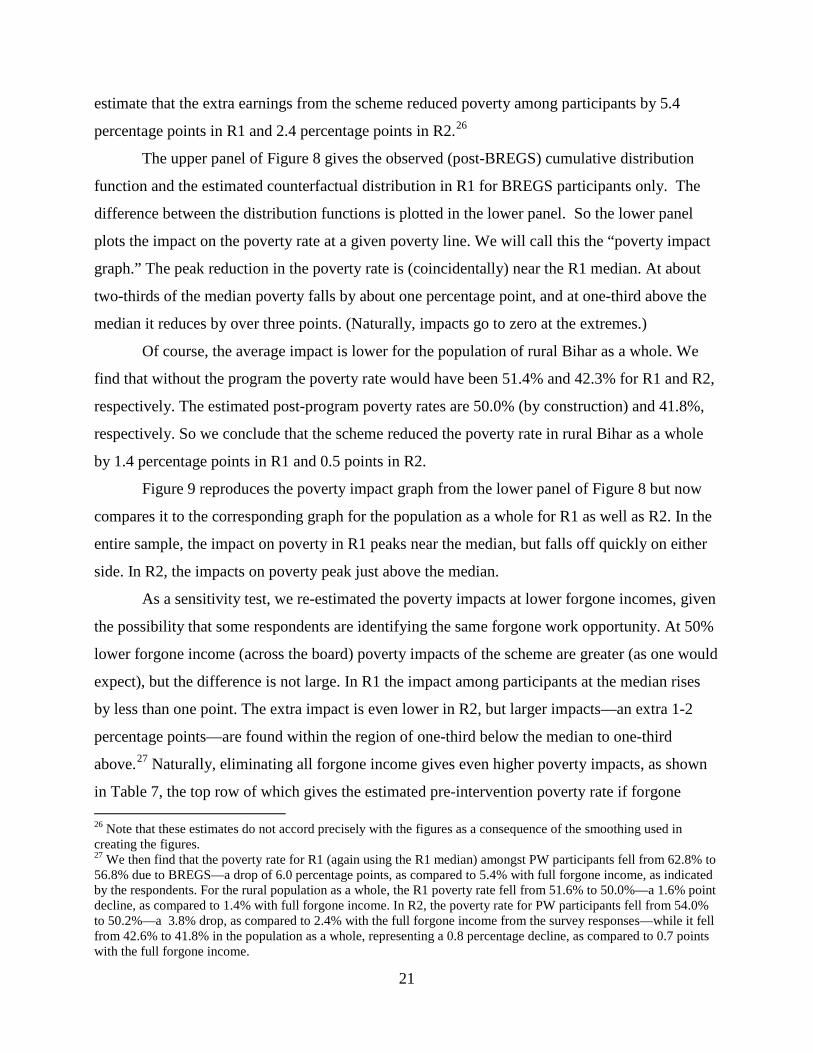
The upper panel of Figure 8 gives the observed (post-BREGS) cumulative distribution

function and the estimated counterfactual distribution in R1 for BREGS participants only. The

difference between the distribution functions is plotted in the lower panel. So the lower panel

plots the impact on the poverty rate at a given poverty line. We will call this the “poverty impact

graph.” The peak reduction in the poverty rate is (coincidentally) near the R1 median. At about

two-thirds of the median poverty falls by about one percentage point, and at one-third above the

median it reduces by over three points. (Naturally, impacts go to zero at the extremes.)

Of course, the average impact is lower for the population of rural Bihar as a whole. We

find that without the program the poverty rate would have been 51.4% and 42.3% for R1 and R2,

respectively. The estimated post-program poverty rates are 50.0% (by construction) and 41.8%,

respectively. So we conclude that the scheme reduced the poverty rate in rural Bihar as a whole

by 1.4 percentage points in R1 and 0.5 points in R2.

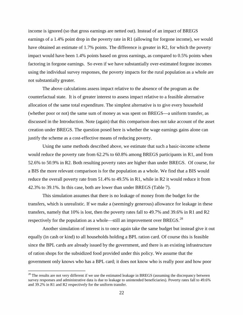
Figure 9 reproduces the poverty impact graph from the lower panel of Figure 8 but now

compares it to the corresponding graph for the population as a whole for R1 as well as R2. In the

entire sample, the impact on poverty in R1 peaks near the median, but falls off quickly on either

side. In R2, the impacts on poverty peak just above the median.

As a sensitivity test, we re-estimated the poverty impacts at lower forgone incomes, given

the possibility that some respondents are identifying the same forgone work opportunity. At 50%

lower forgone income (across the board) poverty impacts of the scheme are greater (as one would

expect), but the difference is not large. In R1 the impact among participants at the median rises

by less than one point. The extra impact is even lower in R2, but larger impacts—an extra 1-2

percentage points—are found within the region of one-third below the median to one-third

above.27 Naturally, eliminating all forgone income gives even higher poverty impacts, as shown

in Table 7, the top row of which gives the estimated pre-intervention poverty rate if forgone 26 Note that these estimates do not accord precisely with the figures as a consequence of the smoothing used in creating the figures. 27 We then find that the poverty rate for R1 (again using the R1 median) amongst PW participants fell from 62.8% to 56.8% due to BREGS—a drop of 6.0 percentage points, as compared to 5.4% with full forgone income, as indicated by the respondents. For the rural population as a whole, the R1 poverty rate fell from 51.6% to 50.0%—a 1.6% point decline, as compared to 1.4% with full forgone income. In R2, the poverty rate for PW participants fell from 54.0% to 50.2%—a 3.8% drop, as compared to 2.4% with the full forgone income from the survey responses—while it fell from 42.6% to 41.8% in the population as a whole, representing a 0.8 percentage decline, as compared to 0.7 points with the full forgone income.

22

income is ignored (so that gross earnings are netted out). Instead of an impact of BREGS

earnings of a 1.4% point drop in the poverty rate in R1 (allowing for forgone income), we would

have obtained an estimate of 1.7% points. The difference is greater in R2, for which the poverty

impact would have been 1.4% points based on gross earnings, as compared to 0.5% points when

factoring in forgone earnings. So even if we have substantially over-estimated forgone incomes

using the individual survey responses, the poverty impacts for the rural population as a whole are

not substantially greater.

The above calculations assess impact relative to the absence of the program as the

counterfactual state. It is of greater interest to assess impact relative to a feasible alternative

allocation of the same total expenditure. The simplest alternative is to give every household

(whether poor or not) the same sum of money as was spent on BREGS—a uniform transfer, as

discussed in the Introduction. Note (again) that this comparison does not take account of the asset

creation under BREGS. The question posed here is whether the wage earnings gains alone can

justify the scheme as a cost-effective means of reducing poverty.

Using the same methods described above, we estimate that such a basic-income scheme

would reduce the poverty rate from 62.2% to 60.8% among BREGS participants in R1, and from

52.6% to 50.9% in R2. Both resulting poverty rates are higher than under BREGS. Of course, for

a BIS the more relevant comparison is for the population as a whole. We find that a BIS would

reduce the overall poverty rate from 51.4% to 49.5% in R1, while in R2 it would reduce it from

42.3% to 39.1%. In this case, both are lower than under BREGS (Table 7).

This simulation assumes that there is no leakage of money from the budget for the

transfers, which is unrealistic. If we make a (seemingly generous) allowance for leakage in these

transfers, namely that 10% is lost, then the poverty rates fall to 49.7% and 39.6% in R1 and R2

respectively for the population as a whole—still an improvement over BREGS.28

Another simulation of interest is to once again take the same budget but instead give it out

equally (in cash or kind) to all households holding a BPL ration card. Of course this is feasible

since the BPL cards are already issued by the government, and there is an existing infrastructure

of ration shops for the subsidized food provided under this policy. We assume that the

government only knows who has a BPL card; it does not know who is really poor and how poor

28 The results are not very different if we use the estimated leakage in BREGS (assuming the discrepancy between survey responses and administrative data is due to leakage to unintended beneficiaries). Poverty rates fall to 49.6% and 39.2% in R1 and R2 respectively for the uniform transfer.

23

they are. So everyone with a BPL card gets the same amount under the counterfactual, and those

without the card get nothing.

We find that this alternative counterfactual would reduce the poverty rate from 51.4% to

49.8% in R1, while in R2 it would reduce the poverty rate from 42.3% to 40.0%. In both cases,

the poverty rates are lower than under BREGS. If we make a 10% allowance for leakage in the

transfers, then the poverty rates fall to 49.9% and 40.2% in R1 and R2, respectively.29

It is notable that, in terms of its impact on poverty, the BPL ration-card counterfactual is

no better than the BIS. This confirms findings from other studies that the targeting of the BPL

cards might be improved.

It should be noticed that with 10% leakage the poverty rate attained by either of these

counterfactual transfer schemes is almost identical to BREGS in R1 (Table 7). This implies that

the workfare scheme would dominate at slightly more than 10% leakage. The gap is somewhat

larger in R2, so greater leakage would be needed to tilt the balance in favor of workfare.

7. Conclusions

While work requirements can ensure good targeting, this probably comes at a cost to poor

participants, notably their forgone earnings. Little is known about these hidden costs. We have

employed a novel survey-based method of measuring these costs at the individual level and used

this in estimating the poverty impacts of a major workfare scheme in rural Bihar, with impacts

assessed against various counterfactuals.

We find that workfare participants are not drawn solely from the pool of the unemployed.

Many report forgone earnings, though mostly a good deal less than the market wage. On average

about one-third of the workfare wage rate is forgone. But the cost of participation varies greatly,

with three distinct groups evident: those with roughly zero forgone income (the largest group),

those for whom the forgone income accounts for around half their workfare wage and those for

whom it is much higher; only for the latter group (the smallest of the three) is the opportunity

cost of workfare labor well approximated by the wage rate for casual market labor.

Factoring in these household-specific opportunity costs, we find that the extra earnings

from this large scheme in Bihar had less impact on poverty than either a basic-income scheme—

29 Again, applying estimated leakage in BREGS yields very similar results. Poverty rates fall to 50.1% and 40.3% in R1 and R2 respectively with a BPL-targeted uniform transfer.

24

providing a uniform transfer of the same gross expenditure to everyone (whether poor or not)—

or a uniform transfer to all those holding a government-issued ration card intended for poor

families. This also holds when we allow for 10% leakage in the transfer schemes, although if

leakage turned out to be much larger than that then workfare would dominate. It is clear,

however, that even in this poor labor-surplus rural economy, the much vaunted self-targeting

mechanism that is achieved by imposing work requirements does not tilt the balance in favor of

unproductive workfare over options using cash transfers with little or no targeting and with up to

about 10% leakage.

Can the scheme be reformed to work better in practice? Forgone incomes are not easily

controlled by such a program. The gaps between the stipulated wage rates and wages received

might be reduced. Pro-poor reform could also reduce the substantial unmet demand for work on

the scheme. This could be done by enhanced public information and a more responsive supply

side; Dutta et al. (2013) identify a number of specific reforms. These would enhance the impact

on poverty though (of course) at a greater cost to the public budget. Cost effectiveness would

need to be reassessed at the implied higher level of funding.

A second direction for reforms is to ensure that workfare is productive—that the assets

created are of value to poor people (or that cost-recovery can be implemented for non-poor

beneficiaries). The creation of durable assets has not had much attention from the scheme’s

advocates and/or administrators. That may need to change. Two qualifications should be noted,

however. First, there may well be a trade-off. Meeting the extra demand for work may well make

it harder to ensure that the assets are indeed of lasting value. The public choice made in response

to such a trade-off will depend on the weight attached to reducing current versus future poverty.

Second, cash transfers can also be used to help create assets—notably in promoting human

capital accumulation by incentivizing schooling and health care for children in poor families,

although for this to work it is crucial that the delivery system for these services is effective. The

cost-effectiveness of “asset-creating workfare” would then need to be compared to such

conditional cash transfers.

25

Figure 1: Delays in BREGS wage payments

Note: Sample restricted to participants who have not been fully paid BREGS wages owed to them. Source: Authors’ estimates based on BREGS Survey.

.1.2

.3.4

.5

shar

e of o

wed w

ages

actua

lly re

ceive

d (%

)

1 2 3 4 5 6 7 8 9 10 11 12number of months since worked

round 1round 2

26

Figure 2: Wages over time in the study villages

Note: The figure reports data on wages owed, based on Block 23 for casual labor done in the week preceding the survey. Wages are nominal. Source: Authors’ estimates based on BREGS Survey.

5070

9011

013

015

0ru

pees

per

day

05

1015

20F

requ

ency

01may2009 01jun2009 01jul2009 01aug2009date of the survey

Public Works

5070

9011

013

015

0ru

pees

per

day

050

100

150

Fre

quen

cy

01may2009 01jun2009 01jul2009 01aug2009date of the survey

Non Public Works

Round 1

5070

9011

013

015

0ru

pees

per

day

010

2030

Fre

quen

cy

28apr2010 13may2010 28may2010 12jun2010 27jun2010date of the survey

Public Works

5070

9011

013

015

0ru

pees

per

day

020

4060

80F

requ

ency

28apr2010 13may2010 28may2010 12jun2010 27jun2010date of the survey

Non Public Works

Round 2

number interviewed wage paid BREGS stipulated wage rate

27

Figure 3: Evolution of BREGS wages and days worked over the entire survey period

Note: Based on individual questionnaire with recall over last year. Wage data reported are household-weighted wages owed to the worker. Source: Authors’ estimates based on BREGS Survey.

20

40

60

80

100

120

140

rupe

es p

er d

ay

05

1015

30da

ys(m

illio

ns)

01jul2008 01jan2009 01jul2009 01jan2010 01jul2010

surveynumber of BREGS days reportedBREGS stipulated wage ratereported BREGS wage rate (female)reported BREGS wage rate (male)

28

Figure 4: Density of daily casual wages, by BREGS participation status

Note: Based on questions about casual work done in the last week. Wage data are unweighted. Source: Authors’ estimates based on BREGS Survey.

0.01.02.03.04

dens

ity

0 50 100 150 200rupees per day

Casual work, all

0.005

.01.015

dens

ity

0 50 100 150rupees per day

Casual work, women

0

.01

.02

.03

dens

ity

0 50 100 150 200rupees per day

Casual work, men

Round 1

0.01.02.03.04.05

dens

ity

0 50 100 150 200rupees per day

Casual work, all

0.01.02.03

dens

ity

0 50 100 150rupees per day

Casual work, women

0

.05

.1

.15

dens

ity

0 50 100 150 200rupees per day

Casual work, men

Round 2

public works wage

non-public works wage: BREGS participants

non-public works wage: BREGS excess demanders

non-public works wage: rest

29

Figure 5: Wages relative to the BREGS stipulated wage rate

Note: Based on questions about casual work done in the last week. Wage data are unweighted. Source: Authors’ estimates based on BREGS Survey.

01

23

4de

nsity

.5 1 1.5ratio of wage rate to BREGS stipulated wage rate

0

.2

.4

.6

.8

1

cum

ulat

ive

dens

ity

.5 1 1.5ratio of wage rate to BREGS stipulated wage rate

Round 1

01

23

45

dens

ity

.5 1 1.5ratio of wage rate to BREGS stipulated wage rate

0

.2

.4

.6

.8

1

cum

ulat

ive

dens

ity

.5 1 1.5ratio of wage rate to BREGS stipulated wage rate

Round 2

non-public works

public works

30

Figure 6: Actual BREGS wages relative to the BREGS stipulated wage rate, by gender

Note: Based on individual questionnaire with recall over the last year. Concerns BREGS only. Source: Authors’ estimates based on BREGS Survey.

0

1

2

3

4

dens

ity

.5 1 1.5ratio of wage rate to BREGS stipulated wage rate

0

.2

.4

.6

.8

1

cum

ulat

ive

dens

ity

.5 1 1.5ratio of wage rate to BREGS stipulated wage rate

Round 1

0

2

4

6

8

10

dens

ity

.5 1 1.5ratio of wage rate to BREGS stipulated wage rate

0

.2

.4

.6

.8

1

cum

ulat

ive

dens

ity.5 1 1.5

ratio of wage rate to BREGS stipulated wage rate

Round 2

Male

Female

31

Figure 7: Distribution of the ratio of self-assessed forgone days to PW days and ratio of

forgone wages to PW wages

Note: These distributions are estimated for all public works at the household level. Source: Authors’ estimates based on BREGS Survey.

0.5

11.5

de

nsi

ty

0 .2 .4 .6 .8 1ratio of foregone days to PW days

0.5

11.5

2de

nsi

ty0 .2 .4 .6 .8 1

ratio of foregone wages to PW wages

round1 round2

32

Figure 8: Impacts on participants' poverty in R1

Cumulative distributions of consumption with and without earnings from public works

Poverty impact graph

Note: A smoothing parameter of 0.3 is used for all figures in this paper. Poverty impact graph is estimated as the difference between the cumulative distribution functions of consumption with and without the program. Source: Authors’ estimates based on BREGS Survey.

0

.2

.4

.6

.8

cum

ulat

ive

dens

ity

1000

5000

1000

069

88

Poverty line

without net earnings from public works with net earnings from public works

-.04

-.03

-.02

-.01

0

Impa

ct o

n po

verty

(cha

nge

in C

DF)

1000

5000

1000

069

88

Poverty line

33

Figure 9: Poverty impact graph for both participants and the whole population

Round 1

Round 2

Source: Authors’ estimates based on BREGS Survey.

-.05

-.04

-.03

-.02

-.01

0

.01

Impa

ct o

n po

verty

(cha

nge

in C

DF)

050

0010

000

1500

020

000

2500

069

88

Poverty line

PW only sample as a whole

-.05

-.04

-.03

-.02

-.01

0

.01

Impa

ct o

n po

verty

(cha

nge

in C

DF)

050

0010

000

1500

020

000

2500

078

36

Poverty line

PW only sample as a whole

34

Table 1: Daily wage rate in Rupees for the week before interview

Mean St.dev. Median N Round 1 All Public works 82.7 27.4 89.0 54 Other casual labor 72.2 31.2 70.0 1031 Men Public works 85.8 25.2 89.0 41 Other casual labor 79.1 29.2 80.0 815 Women Public works 73.0 32.6 80.0 13 Other casual labor 46.0 23.6 45.0 216 Round 2 All Public works 94.8 22.3 100.0 118 Other casual labor 87.2 42.0 100.0 796 Men Public works 99.4 18.2 100.0 75 Other casual labor 97.9 39.3 100.0 574 Women Public works 86.8 26.6 100.0 43 Other casual labor 59.4 35.2 50.00 222

Note: Based on Block 23. We treat wages over 200 or less than 10 Rupees per day as missing values. Wage data are in nominal terms, and reported as unweighted means and medians from the sample. Source: Authors’ estimates based on BREGS Survey.

Table 2: Average wage rates before and after increases in the BREGS stipulated wage

Round 1 Round 2 Public works wage

Non-PW wage

Stipulated BREGS

wage

Public works wage

Non-PW wage

Stipulated BREGS

wage Before increase of stipulated wage mean 80.7 71.4 89.0 93.8 91.5 104.0

s.d. 20.4 30.6 . 24.8 39.8 .

N 46 946 . 54 226 .

t-test: Ho: mean actual wage = stip. wage (prob.)

-2.8 -17.8 . -3.0 -4.7 .

(0.008) (0.000) . (0.004) (0.000) .

After increase of stipulated wage mean 92.2 74.7 102.0 95.5 83.9 114.0

s.d. 32.8 30.1 . 24.3 39.2 .

N 20 377 . 81.0 649.0 .

t-test: Ho: mean actual wage = stip. wage (prob.)

-1.3 -17.6 . -6.9 -19.6 .

(0.199) (0.000) . (0.000) (0.000) .

Note: The wage was increased to Rs 102 on June 16, 2009 in R1, then to Rs 104, and to Rs 114 on May 18, 2010 in R2. T-tests use only daily wages greater than 10 and lower than 200 Rupees/day. Wage data are un-weighted. Source: Authors’ estimates based on BREGS Survey.

35

Table 3: Daily wages for farm and non-farm casual labor in Bihar from 2009/10 NSS, by sub-round

Sub-Round

Agricultural work Manual non-agricultural All operations Cultivation

Mean Median Mean Median Mean Median 1 July-Sept 2009 74.8 77.5 72.4 73.3 86.9 80.0 2 Oct-Dec 2009 72.8 80.0 67.6 70.0 103.4 95.0 3 Jan-Mar 2010 84.6 80.0 80.2 80.0 97.1 90.0 4 Apr-June 2010 86.0 81.4 78.9 80.0 120.7 100.0 Total 79.0 80.0 74.4 76.7 100.2 90.0 Percentage change 1-4 15 5 9 9 39 25

Source: Authors’ calculations from NSS 66th round.

Table 4: Total person days of non-PW work by operation and sub-round 2009/10

Sub-round Manual

agricultural

Manual non-agri

Non-manual non-agri

Missing operation

code All

operations

Household own farm enterprise

1 July-Sept 2009 1340.0 440.0 150.0 21.0 1951.0 2354.0 2 Oct-Dec 2009 1284.5 473.0 324.0 32.0 2120.5 2406.0 3 Jan-Mar 2010 973.0 577.0 235.0 7.0 1792.0 2728.0 4 Apr-June 2010 1035.0 399.5 297.0 7.0 1759.5 2280.5 Total 4632.5 1889.5 1006.0 67.0 7623.0 9768.5

Note: Authors’ calculations from NSS 66th round. Public works excluded. The total for all operations includes some minor omitted categories. Source: Authors’ estimates based on BREGS Survey.

Table 5: Forgone work opportunities identified by BREGS participants

% BREGS participants who say that, if not for BREGS, they would have …

Round 1 Round 2 Men Women Men Women

Migrated for work 10.7 2.9 14.0 1.0 Type of paid work:

Casual work (agricultural) 22.4 24.8 19.4 23.6 Casual work (non-agricultural) 23.8 5.7 25.7 5.0 Other 1.0 0.8 2.1 0.0 Searched for work or remained unemployed 44.0 35.7 37.6 13.2 Worked on own land or house 8.8 33.1 14.9 58.2

100 100 100 100

Notes: The questions were asked of BREGS participants by work episode. The means are formed over all work episodes such that an individual who worked more than once is also counted more than once. Would be migrants are included in totals according to the type of activities they would have done. Source: Authors’ estimates based on BREGS Survey.

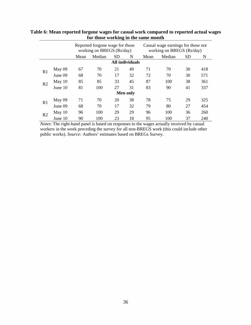
36

Table 6: Mean reported forgone wages for casual work compared to reported actual wages for those working in the same month

Reported forgone wage for those working on BREGS (Rs/day)

Casual wage earnings for those not working on BREGS (Rs/day)

Mean Median SD N Mean Median SD N All individuals

R1 May 09 67 70 21 49 71 70 30 418 June 09 68 70 17 32 72 70 30 571

R2 May 10 85 85 33 45 87 100 38 361 June 10 81 100 27 31 83 90 41 337

Men only

R1 May 09 71 70 20 38 78 75 29 325 June 09 68 70 17 32 79 80 27 454

R2 May 10 96 100 29 29 96 100 36 260 June 10 90 100 23 18 95 100 37 240

Notes: The right-hand panel is based on responses to the wages actually received by casual workers in the week preceding the survey for all non-BREGS work (this could include other public works). Source: Authors’ estimates based on BREGs Survey.

Table 7: Summary of estimated poverty impacts Round 1 Round 2

% below poverty line

Participants only

Population Participants only

Population

Pre-intervention

Estimated by deducting gross earnings gains from BREGS

63.0 51.7 56.4 43.2

Estimated by deducting net earnings gains from BREGS

62.2 51.4 52.6 42.3

Post-intervention

Observed with BREGS 56.8 50.0 50.2 41.8

Counterfactuals for same spending:

Basic-income scheme (BIS) 60.8 49.5 50.9 39.1

BIS with 10% leakage 61.1 49.7 51.0 39.6

Transfers based on ration cards 60.5 49.8 50.1 40.0

Ration card transfers with 10% leakage 60.6 49.9 50.7 40.2

Note: The poverty line is set at the median for R1 as observed (post-intervention).

References

Alik-Lagrange, Arthur and Martin Ravallion, 2012, “Evaluating Workfare when the Work is

Unpleasant,” Policy Research Working Paper 6272, World Bank.

Atkinson, Anthony B., and Holly Sutherland, 1989, “Analysis of a Partial Basic Income

Scheme,” in A.B. Atkinson (ed.) Poverty and Social Security. Hertfordshire: Harvester

Wheatsheaf.

Bardhan, Pranab, 2011, “Challenges for a Minimum Social Democracy in India,” Economic and

Political Weekly 46(10): 39-43.

Berg, Erlend, Sambit Bhattacharyya, Rajasekhar Durgam and Manjula Ramachandra, 2012, “Can

Rural Public Works Affect Agricultural Wages? Evidence from India,” mimeo,

University of Oxford.

Besley, Timothy, and Stephen Coate, 1992, “Workfare vs. Welfare: Incentive Arguments for

Work Requirements in Poverty Alleviation Programs,” American Economic Review

82(1): 249–61.

Besley, Timothy, Rohini Pande and Vijayendra Rao, 2012, “Just Rewards? Locxal Politics and

Public Resource Allocation in South India,” World Bank Economic Review 26(2): 191-

216.

Björklund, Anders, 1987, “What Experiments are Needed for Manpower Policy?” Journal of

Human Resources 23(2): 267-277.

Datt, Gaurav and Martin Ravallion, 1994, “Transfer Benefits from Public Works Employment,”

Economic Journal, 104: 1346-1369.

__________ and ______________, 2002, “Has India’s Post-Reform Economic Growth Left the

Poor Behind,” Journal of Economic Perspectives 16(3): 89-108.

Development Alternatives, 2009, “Report on Scoping Study for Design and Development of

Alternative Implementation Model(s) on NREGS”, background note prepared for the

BREGS study.

Drèze, Jean, 1990, “Famine Prevention in India,” in J. Drèze and A. Sen (eds) The Political

Economy of Hunger, Oxford: Oxford University Press, Volume 2.

_________, 2004, “Employment as a Social Responsibility,” The Hindu, November 22,

(http://www.hindu.com/2004/11/22/stories/2004112205071000.htm)

39

Drèze, Jean and Reetika Khera, 2011, “Employment Guarantee and the Right to Work,” in

Reetika Khera (ed.) The Battle for Employment Guarantee, New Delhi: Oxford University

Press.

Dutta, Puja, Rinku Murgai, Martin Ravallion and Dominique van de Walle, 2012, “Does India’s

Employment Guarantee Scheme Guarantee Employment?” Economic and Political

Weekly 48 (April 21): 55-64.

_________, ____________, ______________and ___________________, 2013, Right-to-Work?

Assessing India’s Employment Guarantee Scheme in Bihar. World Bank Report.

Government of India, Office of the Registrar General & Census Commissioner, 2006,

“Population Projections for India and States 2001-2026, ” Report of the Technical Group

on Population Projections Constituted By the National Commission on Population.

Heckman, James and Richard Robb, 1985, “Alternative Methods for Evaluating the Impact of

Interventions—An Overview,” Journal of Econometrics 30: 239-67.

Heckman, James, Serio Urzua and Edward Vytlacil, 2006, “Understanding Instrumental

Variables in Models with Essential Heterogeneity,” Review of Economics and Statistics

88(3): 389-432.

Imbert, Clement and John Papp, 2011, “Estimating Leakages in India’s Employment Guarantee,”

in Reetika Khera (ed.) The Battle for Employment Guarantee, New Delhi: Oxford

University Press.

_____________ and _________, 2012, “Equilibrium Distributional Impacts of Government

Employment Programs: Evidence from India’s Employment Guarantee,” mimeo, Paris

School of Economics.

Indian Grameen Services, 2010, “Exploring Shelf of Works for Flood Affected area of North

Bihar,” report prepared for the Rural Development Department, Government of Bihar and

the World Bank.

Indian Grameen Services, 2009, “Report on Scoping Study for Design and Development of

Alternative Implementation Model(s) on NREGS and SGSY,” background note prepared

for the BREGS study.

Jalan, Jyotsna and Martin Ravallion, 2003, “Estimating the Benefit Incidence of an Anti-Poverty

Program by Propensity-Score Matching,” Journal of Business and Economic Statistics,

21(1): 19-30.

40

Jha, Raghbendra, Raghav Gaiha, Manoj K. Pandey, 2012, “Net Transfer Benefits under India’s

Rural Employment Guarantee Scheme,” Journal of Policy Modeling 34(2): 296-311.

Khera, Reetika, 2011a, “Wage Payments: Live Without Pay?” in Reetika Khera (ed.) The Battle

for Employment Guarantee, New Delhi: Oxford University Press.

Lewis, Arthur, 1954, “Economic Development with Unlimited Supplies of Labor,” Manchester

School of Economic and Social Studies, 22: 139-191.

Lindert, Peter H., 2013, “Private Welfare and the Welfare State,” in Larry Neal and Jeffrey

Williamson (eds), The Cambridge History of Capitalism, Cambridge: Cambridge

University Press.

Liu, Yanyan and Klaus Deininger, 2013, “Welfare and Poverty Impacts of India’s National Rural

Employment Guarantee Scheme: Evidence from Andhra Pradesh,” Policy Research

Working Paper 6543, World Bank, Washington, DC.

Mann, Neelakshi and Varad Pande, 2012, “Comment on the validity of the claim: MNREGA

builds assets of questionable quality’” Ideas for India (website).

Mathew, George and Nirmala Buch, 2000, Status of Panchayati Raj in the States and Union

Territories of India 2000, Institute of Social Studies, New Delhi.

Meade, James, 1972, “Poverty in the Welfare State,” Oxford Economic Papers 24: 289-326.

Ministry of Labour and Employment, 2010, Report on Employment and Unemployment Survey

(2009-10), Chandigarh: Government of India.

Ministry of Rural Development, 2011, “Reforms in MGNREGA Implementation,” Ministry of

Rural Development, Delhi, India.

Murgai, Rinku and Martin Ravallion, 2005a, “Employment Guarantee in Rural India: What

Would it Cost and How Much Would it Reduce Poverty?” Economic and Political

Weekly, July 30, 2005, pp. 3450-3455.

_____________ and _____________, 2005b, “Is a Guaranteed Living Wage a Good Anti-

Poverty Policy?” Policy Research Working Paper 3460, World Bank.

National Consortium of Civil Society Organizations, 2009, “NREGA Reforms: Building Rural

India,” First Annual Report of the National Consortium of Civil Society Organizations on

NREGA.

National Consortium of Civil Society Organizations, 2011, “MGNREGA: Opportunities,

Challenges and the Road Ahead,” Second Report of the National Consortium of Civil

41

Society Organizations on MGNREGA.

Ravallion, Martin, 1991, “Reaching the Rural Poor through Public Employment: Arguments,

Evidence, and Lessons from South Asia,” World Bank Research Observer, 6: 153-176.

________________, 1999, “Appraising Workfare,” World Bank Research Observer, 14:

31-48.

______________, 2009, “How Relevant is Targeting to the Success of an Antipoverty Program?”

World Bank Research Observer, 24(3): 205-231.

Ravallion, Martin and Gaurav Datt, 1995, “Is Targeting through a Work Requirement Efficient?

“Some Evidence for Rural India,” in D. van de Walle and K. Nead (eds) Public Spending

and the Poor: Theory and Evidence, Baltimore: Johns Hopkins University Press.

Ravallion, Martin, Gaurav Datt, and Shubham Chaudhuri, 1993, “Does Maharashtra’s

‘Employment Guarantee Scheme’ Guarantee Employment? Effects of the 1988 Wage

Increase,” Economic Development and Cultural Change 41: 251–75.

Ravallion, Martin, Emanuela Galasso, Teodoro Lazo and Ernesto Philipp, 2005, “What Can Ex-

participants Reveal about a Program’s Impact?”, Journal of Human Resources. 40: 208-

230.

Ravallion, Martin, Dominique van de Walle, Puja Dutta and Rinku Murgai, 2013, “Testing

Information Constraints on India’s Largest Antipoverty Program, ” Policy Research

Working Paper 6598, World Bank.

Ravi, Shamika and Monika Engler, 2009, “Workfare in Low Income Countries: An Effective

Way to Fight Poverty? The Case of the NREGS in India,” mimeo, Indian School of

Business, Hyderabad.

Raventós, Daniel, 2007, Basic Income: The Material Conditions of Freedom, London: Pluto

Press.

Rosenzweig, Mark, 1989, “Labor markets in developing countries,” in H. Chenery and T.N.

Srinivasan (eds) Handbook of Development Economics, Vol. 1. Amsterdam: North

Holland.

Sunai Consultancy Pvt. Ltd., 2009, “Process Qualitative Observation Report, Feb-Mar 2009, four

blocks of Muzaffarpur and Saharsa districts of Bihar,” background note prepared for the

BREGS study.

Thane, Pat, 2000, Old Age in English History. Oxford: Oxford University Press.

42

van de Walle, Dominique, 1998, “Targeting Revisited,” World Bank Research Observer,

13(2): 231-48.

Vanaik, Anish, 2009, “Accounts of Corruption,” Frontline, Jan.16, p.21.

Verma, Shilp, 2011, MGNREGA Assets and Rural Water Security: Synthesis of Field Studies in

Bihar, Gujarat, Kerala and Rajasthan, Anand: International Water Management Institute

(IWMI).

World Bank, 1986, Poverty and Hunger: issues and Options for Food Security in Developing

Countries. Washington DC: World Bank.

__________, 2004, World Development Report: Making Services Work for Poor People,

Washington DC: World Bank.

Zimmerman, Laura, 2012, “Labor Market Impacts of a Large-Scale Public Works Program:

Evidence from the Indian Employment Guarantee Scheme,” IZA Working Paper 6858,

Bonn, Germany.