Is Who You Work for

as Important as What You Know?

The Role of Firms in Labour Market Outcomes

David Card - UC Berkeley

Economists’ standard prescription for labor market

success: go to school; work hard; acquire new skills...

But if you ask a typical person - getting a “good job”

is the key to success.

Moreover, a lot of local development policies

amount to trying to attract/retain “good jobs.”

What do people mean by a “good job”? Do “good

jobs” come from “good firms”?

Today I will argue that:

a) getting a “good job” is mainly about working

at a “good firm”

b) firms offer systematic wage premiums (or

discounts) relative to “the market”

c) variation in these premiums is large (and growing)

d) more productive firms pay higher wages (there

also may be other sources of variation)

e) firm wage premiums help explain many aspects of

labor market behavior and outcomes

Outline

I. Background

II. How much do firms matter in wage outcomes?

III. Interpretation: rent sharing, efficiency wages or ?

IV. What other features of the labor market can be

explained by firm wage premiums?

cyclical wage variation

career progression

gender gaps

V. What else might be explained?

I. Background

1a. In the standard model we use to study the labor

market (CRS, integrated factor markets) firms don’t

matter

- firms face horizontal supply curves at the market

wage; firm size is indeterminate

- working model for many questions: trade;

immigration; SBTC; human capital; minimum wages;

occupational choice; local labor markets

1b. The “modern” version:

- multiple skill groups; workers perfectly mobile across

firms

- firms differ in various attributes (entrepreneurial

skill, management practices, ...) so there is a lot of

systematic heterogeneity

- But each worker is paid his/her “market wage”.

-No special link to current or past employers

-One good firm benefits all workers in the market

(it doesn’t matter if you actually work for Google)

2. What do we know from earlier work?

a. Research using firm-level union contract data

- rent sharing, pattern bargaining, slow adjustment

b. Research using panel data (PSID, NLSY...)

- big “job component” of wages

c. Research on displaced workers

- job losers have large, persistent wage losses

d. Research on firm-level data sets (LRD...)

- variance in TFP is huge (var=1) and persistent

e. Theoretical research on “frictional markets”

- Burdett Mortensen: firms set wages to balance

turnover costs and wage costs. High/low wages

equally profitable

- DMP: firms post job openings. Workers have

different “match productivities” (each firm has 1 job in

canonical version)

extensions

- Cahuc et al: firms respond to outside offers

- Stole and Zwiebul: individual bargaining

f. Modern rent-sharing literature

- worker-firm data, allows controls for worker

heterogeneity

- very important, since higher skilled workers will

lead to higher value-added/worker (VA/L)

- typical elasticities w.r.t VA/L: 0.05 to 0.10

- CCHK “replication”: look at wage changes of job

stayers in Portugal (QP data) as firm becomes

more/less profitable. Elasticities in same range

Estimated Std. Study and country/industry Elasticity ErrorGroup 3: Firm-level profit measure, individual-specific wage9. Margolis and Salvanes (2001), French manufacturing 0.062 (0.041)9. Margolis and Salvanes (2001), Norwegian manufacturing 0.024 (0.006)10. Arai (2003), Sweden 0.020 (0.004)11. Guiso, Pistaferri, Schivardi (2005), Italy 0.069 (0.025)12. Fakhfakh and FitzRoy (2004), French manufacturing 0.120 (0.045)13. Du Caju, Rycx, Tojerow (2011), Belgium 0.080 (0.010)14. Martins (2009), Portuguese manufacturing 0.039 (0.021)15. Guertzgen (2009), Germany 0.048 (0.002) Mean=0.0816. Cardoso and Portela (2009), Portugal 0.092 (0.045)17. Arai and Hayman (2009), Sweden 0.068 (0.002)18. Card, Devicienti, Maida (2014), Italy (Veneto region) 0.073 (0.031)19. Carlsson, Messina, and Skans (2014), Swedish mfg. 0.149 (0.057)20. Card, Cardoso, Kline (2016), Portugal, between firm 0.156 (0.006)20. Card, Cardoso, Kline (2016), Portugal, within-job 0.049 (0.007)21. Bagger et al. (2014), Danish manufacturing 0.090 (0.020)

Table 1: Summary of Estimated Rent Sharing Elasticities from the Recent (Preferred specification, adjusted to TFP basis)

Table 2: Cross-Sectional and Within-Job Models of Rent Sharing for Portuguese Male Workers

+Major +DetailedBASIC Industry Industry

(1) (2) (3)

B. Within-Job Models (Change in Wages from 2005 to 2009 for stayers)

4. OLS: rent measure = change in log value added 0.041 0.039 0.034 per worker from 2005 to 2009 (0.006) (0.005) (0.003)

5. OLS: rent measure = change in log sales per 0.015 0.014 0.013 worker from 2005 to 2009 (0.005) (0.004) (0.003)

6. IV: rent measure = change in log value added 0.061 0.059 0.056 per worker from 2005 to 2009. Instrument = (0.018) (0.017) (0.016) change in log sales per worker, 2004 to 2010 First stage coefficient 0.221 0.217 0.209

[t=11.82] [t=13.98] [t=18.63

3. Abowd Kramarz Margolis (AKM)

log(wage) = person effect (skills, ambition etc)

+ firm effect (firm-specific premium)

+ Xâ (age/time trends/returns to schooling)

+ error

error = job-match premium + transitory shocks

(firm-wide or worker-specific)

note: job-match Y heterogeneous treatment effect

Reality check - do firms really “post” different wages?

How do firms hire? Hall-Krueger survey

Q1: ‘take it or leave it’ offer or some bargaining?

Q2: knew pay exactly at time of 1st interview

26% pay known/no bargaining

37% pay uncertain/no bargaining

25% pay uncertain/bargaining

Other evidence:

- van Ours and Ridder (inventory of applications)

- job fairs

- network lit: workers know where the good jobs are

Non-parametric evidence of “firm effects”

CHK event study design:

- classify jobs in a year by average coworker wage

(into 4 quartiles)

- select workers who change establishments;

classify changes by quartile of co-worker

wages in last year of old job/first year of new job

- focus on workers with 2+ years pre/post

Mean Wages of Job Changers by Origin/Destination(German FT Men, 2002-2009)

3.6

3.8

4.0

4.2

4.4

4.6

4.8

5.0

5.2

-2 -1 0 1Time (0=first year on new job)

Mea

n Lo

g Re

al D

aily

Wag

e

4 to 4

4 to 3

4 to 2

4 to 1

1 to 4

1 to 3

1 to 2

1 to 1

Mean Wages of Job Changers by Origin/Destination Group(Males, Portugal)

1.0

1.4

1.8

2.2

2.6

-2 -1 0 1Time (0=first year on new job)

Mea

n Lo

g Re

al H

ourly

Wag

e

4 to 4

4 to 3

4 to 2

4 to 1

1 to 4

1 to 3

1 to 2

1 to 1

Closer examination of the wage changes of job

changers (Portuguese male job changers)

- classify jobs into 20 groups using coworker wages

- for each of 400 origin/destination cells calculate

- change in mean log co-worker wage = Äwcoworker

- change in mean wages of movers = Äw

- plot: Äw vs. Äwcoworker

- looks like E[ Äw|Äwcoworker ] = 0.4 Äwcoworker

Wage Changes of Movers vs. Changes of Co-workers(Classifying origin/destination firms into 20 bins)

-1.0-0.8-0.6-0.4-0.20.00.20.40.60.81.0

-2.0 -1.6 -1.2 -0.8 -0.4 0.0 0.4 0.8 1.2 1.6 2.0Mean Log Wage Change of Co-workers

Mea

n Lo

g W

age

Chan

ge o

f Mov

ers

1 3 5 7 9 11 13 15 17 19Origin Group (based on co-worker wages at origin firm):

average slope = 0.43

Take-aways:

1) wages rise/fall when you join a firm with

higher/lower-paid coworkers

2) large gaps - lots of 40% wage losses/gains

3) no average mobility premium

4) approximately symmetric gains/losses

(Y not much sorting on match component)

5) no clear trends in pre/post-transition wages

6) upwardly mobile workers have higher wages

given their origin quartile

(Y sorting on ‘permanent’ ability component)

Applying AKM framework: Germany, Portugal, Brazil

Table 3: Summary of Estimated Models for Male and Female Workers

Males Females German Men Brazil - WMSummary of Parameter Estimates: AKM ModelStd. dev. of pers. effects (person-yr obs.) 0.420 0.400 0.357 0.448Std. dev. of firm effects (person-yr obs.) 0.247 0.213 0.230 0.304Std. dev. of Xb (across person-yr obs.) 0.069 0.059 0.084 0.222Correlation of person/firm effects 0.167 0.152 0.249 0.239Adjusted R-squared 0.934 0.940 0.927 0.899Correlation male / female firm effectsComparison job-match effects model:Adjusted R-squared 0.946 0.951 0.949 0.928

Std. deviation match effect in AKM model 0.062 0.054 0.075 0.120

Share of variance of log wages due to: person effects 57.6 61.0 51.2 44.5 firm effects 19.9 17.2 21.2 20.5 covariance of person/firm effects 11.4 9.9 16.4 14.4 Xb and associated covariances 6.2 7.5 5.2 13.1 residual 4.9 4.4 5.9 7.5

0.590

III. Interpretation

- high-wage firms survive longer

(so they are more profitable, despite higher wages)

- Fr/Italy/PT: premiums correlated with profits

- jobs at high-wage firms survive longer

(wage premium is not just an offset for hours/effort)

- modest widening of premiums over time

BUT: new firms (post-1996) have big lower tail

Y emergence of low wage firms that specialize

in hiring low-wage workers

a. Is the wage premium simply rent-sharing?

- wide variation across firms in profit/worker

(TFP, ...)

- CCHK: relate components of AKM to log(VA/L)

- person effect correlated with VA/L – sorting

- firm effect correlated with VA/L – rent sharing (or?)

- ALSO: check that firm effects for different groups

have similar elasticity

Table 4: Relationship Between Components of Wages and Mean Log VA/N

+Major +DetailedBASIC Industry Industry

(1) (2) (3)

A. Combined Sample (n=2,252,436 person year observations at 41,120 firms)1. Log Hourly Wage 0.250 0.222 0.187

(0.018) (0.016) (0.012)

2. Estimated Person Effect 0.107 0.093 0.074 (0.010) (0.009) (0.006)

3. Estimated Firm Effect 0.137 0.123 0.107(0.011) (0.009) (0.008)

4. Estimated Covariate Index 0.001 0.001 0.001(0.000) (0.000) (0.000)

Table 4: Relationship Between Components of Wages and Mean Log VA/N

+Major +DetailedBASIC Industry Industry

(1) (2) (3)B. Less-Educated Workers (n=1,674,676 person year observations at 36,179 firms)5. Log Hourly Wage 0.239 0.211 0.181

(0.017) (0.016) (0.011)

6. Estimated Person Effect 0.089 0.072 0.069 (0.009) (0.009) (0.005)

7. Estimated Firm Effect 0.144 0.133 0.107(0.015) (0.013) (0.008)

C. More-Educated Workers (n=577,760 person year observations at 17,615 firms)9. Log Hourly Wage 0.275 0.247 0.196

(0.024) (0.020) (0.017)

10. Estimated Person Effect 0.137 0.130 0.094(0.016) (0.013) (0.009)

11. Estimated Firm Effect 0.131 0.113 0.099(0.012) (0.009) (0.010)

IV. What features of the labor market can be

explained by firm wage premiums?

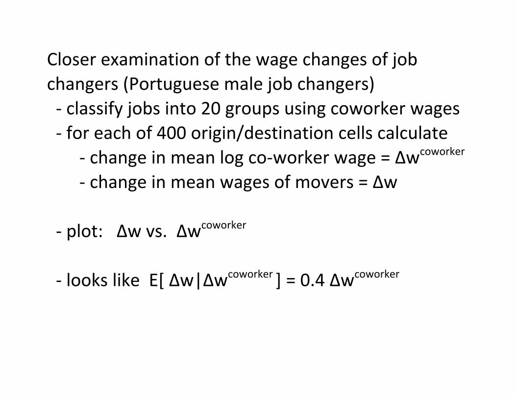
1. Rise in wage inequality (CHK, Germany)

- FT male workers (main job each year) 1985-2009

- compare model in 4 periods:

1985-1991 - before reunification

1990-1996 - reunification, E-W migration

1996-2002 - the “sick man of Europe”

2002-2009 - the German economic miracle

V(log wijt) = V(person) + V(firm) + 2cov(p,f)

+ other components

Trends in Percentiles of Real Log Daily Wages Relative to 1996:Full Time Male Workers in West German Men

-30

-25

-20

-15

-10

-5

0

5

10

15

1985 1987 1989 1991 1993 1995 1997 1999 2001 2003 2005 2007 2009

Year

Valu

e of

Wag

e Pe

rcen

tile

- Val

ue in

199

6

10th Percentile

20th Percentile

50th Percentile

80th Percentile

Decompositions of Rise in Variance for Alternative Samples

FT Males w/FT Men Apprenticeship FT Women

1. Rise in Variance 0.112 0.043 0.095   1985‐91 to 2002‐09

2. Rise in Var(Person Effects) 0.043 0.024 0.048     (percent of total) (39) (55) (50)

3. Rise in Var(Estab. Effects) 0.027 0.018 0.023     (percent of total) (25) (42) (25)

3. Rise in 2×Cov(Pers,Estab) 0.038 0.014 0.017     (percent of total) (34) (32) (18)

2. Gender gap

CCK- Portugal (QP = annual census of all jobs)

fit AKM models separately by gender

counterfactuals:

- raw MF wage gap (hourly wages) = 0.23

- give F’s the male firm effects = 0.22

- give F’s the male firm distribution = 0.18

20-25% of average gender gap is due to firm

distribution

3. cyclical wage variation

some part of cyclical wage adjustment arises from job-

changers

Job changers:

Älog w = Äfirm effects + Ämatch effects

“quality” of new jobs (based on firm effect) is cyclical

Cyclicality in Wage Changes for Continuting and New Jobs (Full Time Males Only)

-4

-3

-2

-1

0

1

2

3

4

5

2003 2004 2005 2006 2007 2008 2009

Mea

n Pe

rcen

tage

Wag

e Ch

ange

s

6

7

8

9

10

11

12

13

14

Une

mpl

oym

ent R

ate

Wage Change, Continuing Jobs

Wage Change, New Jobs

Change in Firm Effects, New Jobs

Unemployment Rate (right scale)

3. Early career progression

- Topel and Ward: young (male) workers’ wages rise

by changing jobs

- does this arise through rising firm quality (as

measured by firm effects), rising match quality, or

both?

- do long term effects of recession (Oreopoulos von

Wachter, Kahn) come from lack of openings at high-

wage firms?

Mean Firm Effects by Age: Portuguese Males

0.0

0.1

0.2

0.3

0.4

19 23 27 31 35 39 43 47 51 55 59 63

Age

Mea

n Fi

rm E

ffect

(Log

Wag

e Sc

ale)

UniversityCompleted High SchoolLower Primary (<5 yrs)

Note: Firm effects are normalized using the method in Card, Cardoso and Kline (2016).

4. wage losses of displaced workers

- seminal JLS study: job losers in PA in early 1980s

losses attributable to disappearing industry rents

(and loss of union coverage)

- Davis + von Wachter: job losers with 3+ years tenure

at plants with 50+ workers that shed 30% or more

workers (not closures).

Earnings Losses (with 0's)

1 yr out 5 yrs out 10 yrs out

avg expansion -10% -6% -4%

avg recession -17% -10% -6%

Contribution of Firm Effects to Wage Changes: Workers Affected by Large Layoff Events, 2004‐2007

‐0.12

‐0.10

‐0.08

‐0.06

‐0.04

‐0.02

0.00

0.02

‐2 ‐1 1 2Years After Event

Relativ

e Da

ily W

age/ Relative Firm

 Effe

ct

Relative Daily Wage

Relative Firm Effect

Full time men with 2+ years of wage data before and after downsizing of 30% or more at firms with 50+ workers

5. Rising returns to education

- CHK find increased sorting of more highly educated

workers to higher-premium firms

- this “explains” all of the rise in return to education in

W. Germany

- can be cross-checked by simple CRE approach:

log wage (i,t) = a(t) + b(t)ED(i,t) + c(t)Co-wkr ED(i,t)

- c(t) and Corr(ED, Co-wkr ED) are is rising over time

- b(t) is actually falling slightly

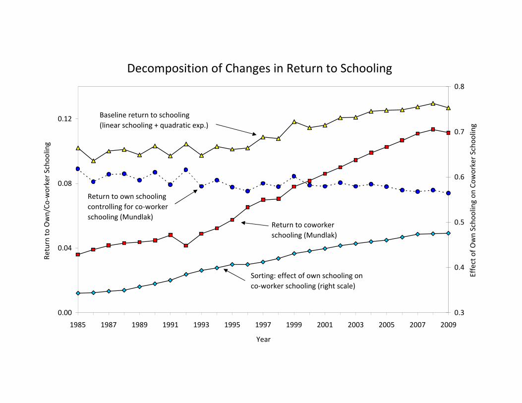
Decomposition of Changes in Return to Schooling

0.00

0.04

0.08

0.12

1985 1987 1989 1991 1993 1995 1997 1999 2001 2003 2005 2007 2009

Year

Retu

rn to

Ow

n/Co

-wor

ker S

choo

ling

0.3

0.4

0.5

0.6

0.7

0.8

Effe

ct o

f Ow

n Sc

hool

ing

on C

owor

ker S

choo

ling

Baseline return to schooling(linear schooling + quadratic exp.)

Return to own schoolingcontrolling for co-worker schooling (Mundlak)

Return to coworkerschooling (Mundlak)

Sorting: effect of own schooling onco-worker schooling (right scale)

V. What else might be related to firm wage

premiums?

1. Other “gaps”

a. racial wage gaps (Brazil)

b. immigrant assimilation (works in Portugal)

c. rise in incomes of the top 1% (Goldman effect)

2. Networks

- network capital = mean(øj) for friends

3. Intergeneration correlation in earnings

(Kramarz-Skans)