Is the Traditional Banking Model a Survivor?

Vincenzo Chiorazzo*, Italian Banking Association Vincenzo D’Apice*#, Italian Banking Association

Robert DeYoung, Kansas University Pierluigi Morelli*, Italian Banking Association

Istituto Einaudi for Banking, Finance and Insurance Studies IstEin Research Paper #13

This version: February 5, 2016

Abstract: We test whether relatively small US commercial banks that use traditional banking business models are more likely to survive during both good and bad economic climates. Our concept of bank survival is derived from Stigler (1958), and includes any bank that did not fail, was not acquired, and was not absorbed into its parent holding company. Our concept of traditional banking is based on four hallmark characteristics of this business model: Relationship loans, core deposit funding, revenue streams from traditional banking products and services, and physical bank branches. We find that banks that adhered more closely to this business strategy were an estimated 13 percentage points more likely to survive from 1997 through 2012 than banks that used less traditional business strategies. Importantly, the estimated traditional bank survival advantage approximately doubled during the 2006-2012 crisis period compared with the relatively stable 1997-2006 pre-crisis years.

* The views expressed in this study are not necessarily those of the Italian Banking Association. The authors are grateful for the comments and suggestions received during presentations at the European Financial Management Association and the Southern Finance Association. # Corresponding author: Vincenzo D’Apice, Italian Banking Association, v.dapice@abi.it.

1

1. Introduction

The global financial crisis of 2007-2009 resulted in severe financial distress, insolvency, and

in some cases government bailout, for thousands of banking companies in Europe and the US. Looking

back at this episode, research has focused nearly exclusively on the question “What went wrong?” The

conclusions of these studies—on the causes of bank insolvency, illiquidity, and systemic risk—have

helped shape reforms in bank regulation aimed at reducing the likelihood of similar episodes in the

future. This is a logical and well-worn approach, and it mirrors the ways that researchers and

policymakers have proceeded in the wake of previous banking crises. But this is also an incomplete

approach. Rather than focusing only on “What went wrong?” and then prescribing policies that attempt

to prevent banks from repeating those mistakes, why not also attempt to identify “What went right?”

and then encourage banks to embrace those positive practices?

On its surface, the financial crisis provided additional support for the conventional narrative

that small commercial banking companies are dinosaurs destined for extinction from banking markets.

Of the 521 US banks that have failed or required government financial assistance since 2007, 502 were

small, so-called ‘community banks’ with assets less than $10 billion.1 This is consistent with a secular

decline in the population of community banks prior to the financial crisis. Between 1984 and 2007, the

number of community banks in the US declined by roughly half, caused by bank failures, bank mergers

and acquisitions, and bank holding company reorganizations.

Nevertheless, approximately six thousand community banking organizations remain in

operation in the US (FDIC 2012). What went right for these banks? In this study, we focus on the

business models used by US community banks, carefully differentiating banks that exhibit ‘traditional’

banking characteristics from banks that do not. We then test whether community banks that used a

more traditional banking approach—that is, banks that relied primarily on relationship lending, core

deposit funding, balance sheet and other traditional sources of revenue, and physical branch

1 Data from the Federal Deposit Insurance Corporation website (www.FDIC.gov) for January 2008 through April 2015. The reported result is based on the broad definition of a community bank that we use in this study, which includes banks with less than $10 billion in assets. Based on a more conservative asset size threshold of $2 billion, 477 of the 521 failed banks were community banks.

2

distribution—have been more or less likely to survive than other community banks, both through good

economic times and bad economic times.

Our investigation is in the spirit of Stigler’s (1958) survivorship concept, in which a researcher

allows the natural outcomes from competitive marketplaces reveal successful and unsuccessful business

practices. The approach is simple and straightforward: A bank is identified as a ‘survivor’ if, at the

end of some measured time period, it is still operating. The survivorship concept makes no distinctions

among the various avenues that a bank might use to exit the market, because all avenues of exit indicate

that a bank either did not or could not survive on its own. A financial failure (i.e., a bank that disappears

due to insolvency or illiquidity) is treated no differently than a strategic failure (i.e., a bank that

disappears as the target in a merger, acquisition or holding company reorganization). We apply this

concept to a large dataset of US commercial banks between 1997 and 2012. We observe which banks

survived during the relatively strong 1997-2006 economic climate; which banks survived during the

more stressful 2006-2012 economic climate; and then test whether banks that used traditional banking

business models exhibited especially strong or especially weak survivorship through either or both of

these time periods.

Because our objective is to determine whether the traditional banking business model is a

survivable model, we exclude from our analysis banks that are either too small or too large to fully

capture the strategic advantages of traditional banking. We limit our focus to banks with between $500

million and $10 billion of assets (2006 dollars). Previous research suggests that banks with assets less

than $500 million face a competitive disadvantage regardless of their business model; they are too small

to survive in truly competitive markets because they leave a substantial portion of available scale

economies unexploited (DeYoung 2013a). At the other extreme, a bank can be too large to profitably

establish and maintain the person-to-person relationships with depositors and borrowers that are central

to the traditional banking business model. There is no extant research on the size at which banks using

the traditional banking model begin to encounter diseconomies of scale; researchers and regulators have

for many decades simply used $1 billion of assets as a convenient upper bound for defining community

banks. We expand this upper bound to $10 billion to account both for inflation and for technological

advances (e.g., cell phones, the Internet) that have enhanced banks’ abilities to maintain person-to-

3

person contact at longer distances (Berger and DeYoung 2006).2 We employ standard data selection

protocols in our statistical tests to control for any bias that may result from our ex ante decision to

restrict the sizes of the banks included in our analysis.

We define a bank as ‘traditional’ if it falls within the $500 million to $10 billion of assets size

range and has higher-than-median values for three of the following four variables: Relationship loans-

to-assets; core deposits-to-assets; branches-to-assets; and the percentage of its operating revenues

generated from traditional banking products and services. We find strong evidence that this combined

set of attributes is associated with bank survival. All else held equal, a so-defined traditional bank was

an estimated 13 percentage points more likely to survive from 1997 through 2012, relative to a

nontraditional bank. Importantly, the survival advantage of the traditional banking model became much

stronger during the financial crisis when bank balance sheets came under substantial stress.

Performing our analysis for US banks gives us access to especially rich data on the financial

and strategic details of thousands of small banks competing in hundreds of different local markets. But

banking technologies and competitive business strategies migrate easily across national borders, and

the regulatory practices of different countries have been converging over time. Hence, what we learn

here about the survivability of relatively small US banks should also hold in large part for the

survivability of similarly sized banks in other countries.

The remainder of the paper is organized as follows. In section 2 we review the previous studies

that are most relevant for our analysis. In section 3 we describe our basic research methodology and

describe how we select our sample of US community banks. In section 4 we examine the strategic and

financial attributes of these banks, and explore which of these attributes were most closely related to

banks’ surviving our 1997-2012 sample period. In section 5 we draw our distinction between traditional

and nontraditional banks, and perform simple survivorship tests in the spirit of Stigler (1958). In section

6 we extend our analysis to include more sophisticated multivariate econometric models. Section 7

summarizes and concludes.

2 Banks with assets in excess of $10 billion eventually gain access to high-volume, repetitive-use production processes—such as credit-scored lending, asset securitization, and online payments services—that drive down their per unit costs dramatically. For banks that are large enough to fully exploit these production processes, the traditional in-person relationship banking approach is simply not cost competitive.

4

2. Literature Review

The central concept in this study is bank survival, that is, whether a bank that is operating at

the beginning of some pre-determined time period is still operating at the end of that time period. In

our analysis, the manner in which the non-surviving banks disappear is immaterial; we treat exit via

insolvency (financial failure) and exit via acquisition (strategic failure) identically. We are interested

in what allows banks to survive: Non-surviving banks will not be around to provide financial services

next year, regardless of how they passed away, but surviving banks will.

This perspective is unique in the bank failure literature, which focuses squarely on bank exit.

There is a large body of research on bank financial failure, driven by the needs of bank supervisors,

regulators, and lawmakers to understand whether and how banking crises can spill over into the macro-

economy. There is also a large body of research on what we refer to here as bank strategic failure, in

which banks are targeted and taken over by other banks. The inference here is that the acquired bank

may have been financially healthy, but its business model, geographic location, management team, or

other characteristics made the bank less valuable on its own than as part of the bank that acquired it. A

small handful of studies jointly examine both financial failure and strategic failure.3

Our brief review of the bank exit literature is not meant to be all inclusive. We want to illustrate

that the extant literature on bank exit is bifurcated into a financial failure subgroup and a strategic failure

subgroup. And we want to identify the determinants of bank exit that overlap in these two sets of

studies, as these are likely to be the results most instructive for determining the causes of bank survival.

2.1. Exit by financial failure

The first bank failure studies documented the wave of US bank and thrift failures in late 1980s

and early 1990s. These studies were characterized as ‘early-warning’ models for preemptively

detecting potential financial distress, thus allowing bank supervisors to attempt corrective actions. This

set of studies includes, among many others, Thomson (1991), Whalen (1991), Cole and Gunther (1995),

Wheelock and Wilson (2000), DeYoung (2003b), Oshinsky and Olin (2006) and Schaeck (2008). This

3 One such example is DeYoung (2003a).

5

body of research collectively identified a standard set of variables useful for predicting bank financial

distress and failure, including rapid loan growth, overreliance on loans backed by commercial real

estate, and heavy use of wholesale funding and interbank funding sources.

A second and more recent set of studies documented bank failures during the more recent

financial crisis. In particular, many of these studies tested whether banks’ expansion into nontraditional

banking activities influenced bank failure probabilities. Cole and White (2012) found that so-called

‘toxic’ investments in mortgage-based securities (MBS) were not significant predictors of individual

bank failures in the US during the financial crisis; these authors showed that the primary drivers of

crisis-era bank failures were strikingly similar to the primary drivers of bank failures during the 1980s

and 1990s, namely, high concentrations of commercial real estate and construction loans. Antoniades

(2015) showed that increased investment in private-label (typically riskier) MBS prior to the crisis

significantly increased the chances of bank failure during the crisis, but increased investment in agency

(typically safer) MBS had no similar effect. After controlling for the traditional balance sheet drivers

used in previous studies, DeYoung and Torna (2013b) tested whether bank participation in less

traditional noninterest-bearing activities increased the probability of failure. These authors found that

income from fee-for-service activities (e.g., mortgage servicing, securities brokerage, insurance sales

and other activities that do not require banks to hold risky assets) helped prevent financially distressed

banks from failing, while stakeholder activities (investment banking, venture capital, proprietary trading

or other activities that often do require banks to hold risky assets) helped banks avoid financial distress

but accelerated failure for banks that did become distressed.

2.2. Exit by strategic failure

When a bank wishes to grow, it has two choices: It can expand internally which tends to be a

slow and gradual process, or it can expand via acquisition which holds the promise of fast and

immediate results. Unlike internal expansion, in which a bank grows by scaling up its existing business

model (i.e., its mix of inputs, outputs, and managerial practices), expansion via acquisition grafts an

outside business model onto an existing bank. To avoid post-acquisition frictions, it follows that an

acquisitive bank will take great care when evaluating the characteristics of its potential target banks.

6

Researchers have identified a number of desirable and undesirable target bank characteristics.

Wheelock and Wilson (2004) and Akhigbe, Madura and Whyte (2004) found that the chances of a US

bank being acquired is higher if the target bank is relatively less profitable than the acquiring bank. An

earlier study by Wheelock and Wilson (2000) found that banks with lower capital ratios are more likely

to be acquisition targets. These studies suggest the existence of an efficient market for corporate control

in which well-run banks purchase poorly run banks and put the acquired resources to more productive

uses. Studies of European bank mergers have found similar results. Beitel, Schiereck and Wahrenburg

(2004) and Pasiouras, Tanna and Zopounidis (2007) showed that targets are less cost- or profit-efficient

than acquirers on average. Focarelli, Panetta and Salleo (2002) found that targets in Italian bank

acquisitions have relatively poor credit management, and that bank M&As tend to result in improved

credit allocation and loan portfolio quality.

There are also some counter-results. Valkanov and Kleimeier (2007) examined large bank

deals in the US and Europe between 1997 and 2003; they found little difference in the capital strength

of European banks engaged in M&A activity, and they found that US target banks tended to be more

highly capitalized than their acquirers. In a study of distressed and non-distressed German bank

mergers, Koetter, et al. (2007) found relatively poor financial performance at highly acquisitive banks.

Hosono, Sakai and Tsuru (2006) studied bank mergers in Japan, and found that cost- and profit-

inefficient banks were the banks most likely to engage in M&A activity.

2.3. Bank success during the financial crisis.

We are unaware of any academic or regulatory studies that focus explicitly on bank survival—

that is, the complement of bank exit—nor any studies that, in this context, explicitly model or quantify

the traditional banking business model. However, two recent studies looked at US banks that performed

especially well during the financial crisis, and attempted to isolate the determining factors.

Brastow, et al. (2012) conducted in-depth interviews with nine small US banks in the Fifth

Federal Reserve District that maintained high supervisory safety and soundness ratings from 2000

through 2011. The interviews revealed, among other things, a commitment to “conservative business

models” based on relationship banking, careful loan underwriting, and slow growth. In addition, the

authors compared these nine healthy banks to eight Fifth District banks of similar sizes that lost their

7

high supervisory ratings during the financial crisis. The healthy banks were more reliant on core deposit

funding, had less concentrated (i.e., more diversified) loan portfolios, and made fewer commercial real

estate loans. Gilbert, Meyer and Fuchs (2013) used a similar research method, but focused on a much

larger sample of 702 “thriving” US community banks that maintained the very highest supervisory

rating every year from 2006 through 2011. They compared these thriving banks to 4,525 community

banks that operated from 2006 through 2011 with lower supervisory ratings, and found results largely

consistent with the earlier study by Brastow, et al. (2012). On average, the thriving banks exhibited

slower asset growth, were more reliant on core deposit funding, made fewer commercial real estate

loans, and maintained greater asset liquidity (lower loan-to-assets ratios). Based on follow-up telephone

interviews with 28 of the thriving banks, the authors were unable to find any overarching consistency

across the business strategies of these banks.

3. Methodology and Data

Our objective is to determine whether the traditional commercial banking model remains

financially viable today and in the near future. Financial viability has two components: Generating a

competitive return for bank equity investors across all phases of the business cycle, and withstanding

external shocks that can occur during some phases of the business cycle. Our methodology is based on

the logical argument that a commercial firm must possess both of these characteristics to continue to

exist as an independent entity across the business cycle. We accept not failing and not being acquired—

that is, surviving—as prima facie evidence of financial viability.

Apart from this conceptual framework, which flows from Stigler (1958), our study is a purely

empirical investigation. The simple approach that we use here has three main virtues. First, it is a

theoretically sound but non-technical approach that is transparent and easily accessible to bankers, bank

analysts, and bank policymakers. Second, the analysis relies on observable marketplace outcomes

rather than estimated relationships or extrapolated trends. Third, to the best of our knowledge, this

approach has never before been applied to banking industry data, and hence it may yield new insights.

We apply our methodology to US commercial banks between 1997 and 2012. We proceed in

three steps. We begin by selecting a sample of US banks in 1997 that were large enough, but not too

8

large, to employ the traditional banking business model with a reasonable expectation of long-run

financial viability. The vast majority of US banks use some version of the traditional banking model,

but most of these banks are arguably too small for long-run viability in competitive banking markets.

Insufficient size can reduce a bank’s ability to survive external shocks or earn a competitive return—

not because the traditional banking model is non-viable, but because the bank using it is too small to

capture all of the scale economies associated with this model.4 Excessive size also reduces the long-

run viability of the traditional banking model, because maintaining the person-to-person relationships

upon which the traditional banking model is predicated becomes increasingly difficult with the

organizational complexity necessary in a large bank. Based on patterns of survival that we observe in

the data (see Figure 1), we restrict the size of our sample to banks between $500 million and $10 billion

in assets in 1997.

With this sample of banks in-hand, we then attempt to identify the set of bank characteristics

(e.g., business mix ratios, financial performance ratios, risk ratios) in place at the beginning of our 1997-

2012 sample period that are most strongly predictive of bank survival through the entire sample period.

As discussed above, we define survival in the Stiglerian sense of not exiting the market for any reason

whatsoever during a given period of time: The bank did not fail, it was not acquired by another bank,

it was not absorbed by an affiliated bank during a holding company reorganization, etc. Using simple

difference-in-means tests, we compare the average values of each bank characteristic (say, the loans-

to-assets ratio) just prior to 1997 for banks that did and did not survive until 2012. We examine 19

different bank characteristics (expressed as financial ratios), paying special attention to the

characteristics associated with the traditional banking business model.

Finally, we construct a traditional banking index based on a subset of four characteristics central

to traditional commercial banking, and we test whether banks with high values of this index are more

likely to survive than banks with low values of this index. The four key characteristics are: (1) a high

percentage of bank assets are relationship loans, (2) a high percentage of bank assets are funded using

4 A clear exception to this are small banks that operate in rural geographic markets where weak local market competition provides pricing power. Barring entry from larger out-of-market banks, small rural banks are viable despite their inefficiently small scale.

9

relationship deposits, (3) a high percentage of bank income comes from traditional banking activities,

and (4) a high reliance on a traditional branch distribution system. We perform these tests using

univariate difference-in-difference tests, multivariate cross sectional estimations, and multivariate panel

estimations.

3.1. Data selection

We construct our dataset from three sources. For US banks that are organized as part of a

holding company structure, we collect balance sheet and income statement data from the FR Y-9C

database, which is collected and made public by the Federal Reserve. These data consolidate the

financial statements of all the commercial banks that operate within a single bank or financial holding

company. For US banks that are not organized as part of a holding company, we collect balance sheet

and income statement data from the Reports of Condition and Income database, which is collected and

made public by these banks’ primary federal supervisors—either the Federal Reserve (Fed), the Office

of the Comptroller of the Currency (OCC), or the Federal Deposit Insurance Corporation (FDIC). For

all banks and bank holding companies, we collect data on banks’ branch networks and the geographic

distribution of a bank’s depositors from the FDIC’s Summary of Deposits database. (For the remainder

of this study, we will use the words “bank” and “banking company” interchangeably to refer to the

firms in our data, regardless of their organizational form.)

At year-end 1997 there were 9,050 commercial banking companies (by our definition)

operating in the United States.5 We excluded a total of 2,162 of these banks from our dataset for the

following reasons: 591 of these banks had foreign ownership greater than 50%; an additional 927 banks

did not report complete balance sheet data; an additional 63 banks invested less than 10% of their assets

in loans to households and businesses; an additional 27 banks used deposits to fund less than 2% of

their assets; an additional 398 banks were less than 5 years old; and an additional 156 were multi-bank

holding companies (MBHCs) that were themselves subsidiaries of other MBHCs. Thus, we begin our

analysis with 6,888 banks at year-end 1997.

5 1,577 of these banks were multi-bank holding companies (MBHCs), 4,488 were one-bank holding companies (OBHCs), and 2,985 were independent or free-standing banks (FSBs).

10

Only 4,164 of these banks survived (by our definition) until year-end 2012. The 2,724 non-

survivors are distributed as follows: 1,899 were healthy banks acquired by other banks; 281 were

declared failures by their primary supervisors and were seized by the FDIC;6 468 were transformed

from banks to branches in holding company reorganizations;7 73 banks were voluntarily closed or

liquidated by their owners; and we determined that 3 banks would have failed had they not received

Troubled Asset Relief Program (TARP) capital injections.8 Thus, the 4,164 survivors were financially,

strategically or operationally strong enough to remain in the marketplace on their own from 1997

through 2012. These data are presented in Table 1.

From these 6,888 survivor and non-survivor banks, we focus our tests on a final sample of 546

banks with between $500 million and $10 billion of assets at year-end 1997. These banks are especially

suitable for our analysis. Previous research suggests that banks with less than $500 million of assets

are substantially less likely to survive in competitive markets, because they leave a substantial portion

of available (cost or revenue) scale economies unexploited (DeYoung 2013a). In other words, these

banks face a competitive disadvantage based on their size, regardless of their business model. There

are also reasons to believe that a bank can become too large to effectively implement the traditional

banking model, which by definition requires banks to establish in-person relationships with their retail

and small business borrowers and depositors. While these relationships become more difficult to

initiate and maintain as a bank grows larger, there is no definitive size at which a bank becomes ‘too

large’ to be a successful traditional bank. Since at least the 1980s, researchers and regulators have used

$1 billion as a convenient upper bound for defining a community bank. We make two adjustments to

this number. First, to account for inflation, we double this crude threshold to $2 billion. Second, to

account for technological change since the 1980s, we further (and arbitrarily) expand this upper bound

6 The FDIC has a variety of resolution methods for the failed banks that it seizes. Of the 281 banks that failed during 1997-2012, the FDIC arranged 183 acquisitions by other banks along with financial assistance, arranged 91 acquisitions by other banks without financial assistance, and liquidated the assets of 7 failed banks. 7 337 of these banks disappeared when OBHCs became part of a MBHC, 105 FSBs disappeared when they became part of a MBHC, and 26 banks disappeared for other reasons. 8 We tracked all 263 of the banks in our sample that received a TARP capital injection, beginning in the quarter t in which their received the equity injection. If the private equity position of these banks (i.e., total equity capital minus the amount injected by the government) became negative in any future quarter t+s, then we assumed that the bank would have failed but for the government assistance.

11

to $10 billion.9 Because this ex ante selection process may influence our estimates, we employ standard

protocols for selection bias in our econometric tests.

Figure 1 provides support for our selection decision. The US commercial banking industry

consolidated substantially over the course of our 1997-2012 sample period, with the number of

separately chartered US commercial banks declining by about one-third. The figure shows how this

consolidation impacted the asset size distribution of US banks. The number of banks with between

$500 million and $2 billion in assets increased by 21%, and the number of banks with between $2

billion and $10 billion in assets increased by 14%. The number of banks in all of the remaining size

categories declined, in some cases substantially. The large reduction in the number of banks populating

the smallest size classes is Stiglerian-type evidence of suboptimal scale: When industry deregulation

during the 1980s and 1990s exposed these small banks to increased competition, many of these banks

became unprofitable and exited the industry.10 The large reduction in the number of banks populating

the largest size classes is evidence of already large banks combining with each other to achieve the even

larger size necessary to fully exploit the new transactions-based banking model. The $500 million to

$10 billion size range appears to be a safe harbor in between these two extremes. Within this size range,

we should be able to test more cleanly the viability of the traditional banking model, relatively

unaffected by the transitory issues of deregulation, suboptimal bank size, and the pressure to either

acquire or be acquired.

4. Univariate survival analysis

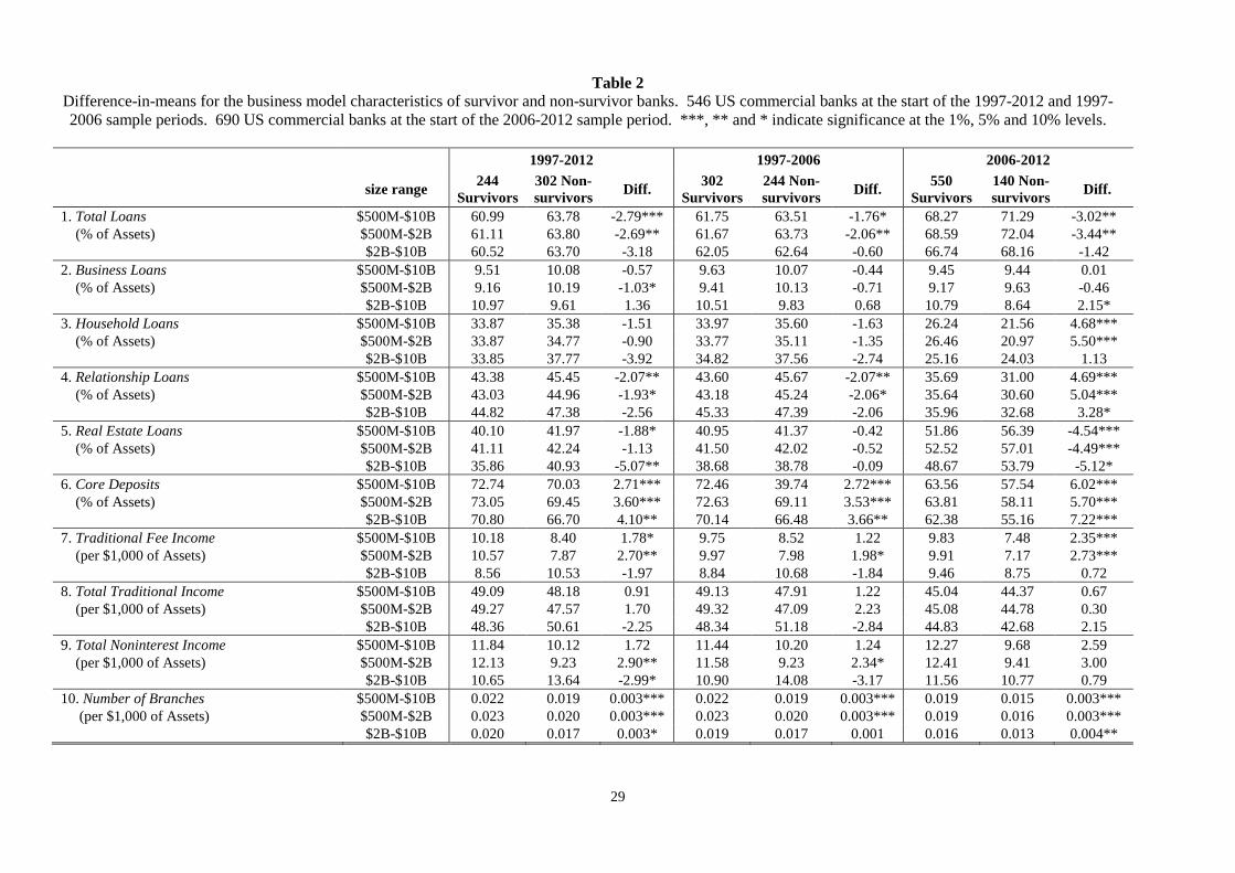
Of the 546 banks in our final sample, 244 banks survived the entire 1997-2012 sample period

and 302 banks did not. In Tables 2 and 3 we use difference-in-means tests to compare the survivor

banks and non-survivor banks across 19 different business activity, financial performance, and financial

risk ratios. (Detailed definitions and summary statistics for each of these ratios are provided in

9 New communications technologies (e.g., cell phones, online banking) have enhanced banks’ abilities to maintain person-to-person relationships at longer distances. New information and financial technologies (credit scoring, loan securitization) have created a new banking model in which very large banks can profitably abandon relationship banking in favor of high volume, repetitive transactions that sharply drive down per unit costs. 10 State and federal regulations that for decades had shielded small banks from out-of-market competition were gradually removed during the 1980s and 1990s.

12

Appendix Table A1.) Because the $10 billion upper asset size threshold is a somewhat arbitrary choice,

we perform the difference-in-means tests for banks in three different size groups: The full sample of

banks with $500 million to $10 billion in assets; the smaller banks in the $500 million to $2 billion

subsample; and the larger banks in the $2 billion to $10 billion subsample. Because bank policymakers

are especially interested in the survival of banking companies during turbulent economic times, we

repeat all of these difference-in-means tests for two sub-periods: The relatively stable 1997-2006 time

period and the relatively stressful 2006-2012 financial crisis period. To partially mitigate survivor bias

in the 2006-2012 subsample tests, we draw a new sample of 690 US commercial banks with assets

between $500 million and $10 billion at year-end 2006.11 Thus, there are nine separate difference-in-

means tests in each of the 19 panels. In all nine sets of tests, we use two-year averages for the activity,

performance, and risk ratios being tested, calculated using data from the two years just prior to the

beginning of the time period over which we are measuring survival.12

Before discussing the individual results of these tests, we note that the $2 billion to $10 billion

subsample (third row of each panel) yields relatively few statistically significant differences between

survivor and non-survivor banks. One plausible explanation is that banks’ activities—and hence banks’

financial performances—grow more homogeneous as banks get larger, leaving less scope for marked

differences across surviving and non-surviving banks. Another plausible explanation is that the

relatively smaller number of observations in this subsample simply reduces statistical precision. In any

case, we focus our analysis on the full sample of banks (the first row) and the $500 million to $2 billion

subsample of banks (the second row) in each panel.

4.1. Business activities

In Table 2 we compare the business activities of survivor and non-survivor banks. We begin

with banks’ loan portfolios. The data for Total Loans (panel 1) are consistent with a familiar story. By

approving rather than rejecting the marginal loan application, banks can increase their short-term

11 The year-end 2006 sample of 690 banks is drawn using the same sampling techniques and thresholds used to draw the year-end 1997 sample of 546 banks. The 2006 sample contains more banks, chiefly because real asset growth between 1997 and 2006 that pushed banks across the $500 million lower bound. 12 Using data from two years reduces the impact of unusually high or low one-year values. For the 1997-2012 and 1997-2006 test periods, we use year-end 1996 and year-end 1997 data. For the 2006-2012 test period, we use year-end 2005 and year-end 2006 data.

13

earnings, but this aggressive lending strategy usually increases credit risk exposure over the longer term.

On average, non-surviving banks were more aggressive lenders, making $2.79 more loans per $100 of

assets than surviving banks.

The composition of banks’ loan portfolios also matters. Relationship lending is one of the

hallmark characteristics of the traditional banking business model. Of course, the financial data do not

allow us to perfectly separate relationship loans from non-relationship loans. We define Relationship

Loans (panel 4) as the sum of Business Loans (panel 2) and Household Loans (panel 3). Business loans

includes all commercial and industrial loans that are not secured by real estate; for the relatively small

banks in this study, these consist almost entirely of loans to small and privately held businesses for

which a close bank-borrower relationship is a given. Household loans includes consumer loans (e.g.,

credit card, auto, home equity) and residential mortgages; the fact that these loans are held on banks’

balance sheets, as opposed to being sold into loan securitizations, is a strong indication that banks seek

to maintain or develop a relationship with these borrowers. Thus, the Relationship Loans variable is

likely associated with a bank’s ability to glean useful information from in-person relationships, and as

such be associated with positive loan portfolio performance. In contrast, Real Estate Loans captures

loans made to businesses secured by the value of underlying real estate; this includes commercial real

estate loans, construction and development loans, and commercial mortgage loans (panel 5).

Fluctuations in local real estate prices have a large influence on the performance of these loans, even if

an in-person relationship exists between the borrower and the bank.

Heading into 2006, banks that ultimately survived the crisis period were holding $4.69 more

relationship loans (by our definition) per $100 of assets than banks that did not survive the crisis, but

$4.54 fewer real estate-backed loans per $100 of assets.13 This is consistent with the findings of Cole

and White (2012), who show that high concentrations of real estate-backed commercial loans and real

estate-backed construction and development loans were positively associated with bank failure during

13 We note that the $4.69 Relationship Loans result is driven solely by the Household Loans ratio (panel 3); the Business Loans ratio (panel 2) is by itself unrelated to survival in any of the time periods in Table 2. This is not surprising. For household lending, a small bank can choose between the traditional relationship-based strategy or the nontraditional loan securitization strategy. But for business lending, all small banks, regardless of strategy, have access only to small business loans, which be definition require a relationship-based approach.

14

both the financial crisis of 2007-2009 and the bank failure wave of the late 1980s and early 1990s. In

contrast, banks that survived the less stressful 1997-2006 period held $2.07 fewer relationship loans per

$100 of assets—this stark difference reminds us of the point made earlier, that the financial viability of

a business model depends on its ability to withstand external shocks across all phases of the business

cycle.

Another hallmark characteristic of the traditional banking model is the use of relationship

deposits to fund bank assets. This approach both reduces bank funding costs and reduces bank liquidity

risk, because depositors that have a relationship with their banks are more likely to maintain high deposit

balances even if they are paid a below-market interest rate. We use Core Deposits as a proxy for

relationship deposits (panel 6). The benefits of this funding approach show up throughout the business

cycle but especially during the crisis period. Heading into 1997, banks that survived until 2012 were

using $2.71 more core deposits per $100 of assets than non-survivors; heading into 2006, banks that

survived until 2012 were using $6.02 more core deposits per $100 of assets than banks that did not

survive the crisis.

By definition, a traditional bank will generate the lion’s share of its income from traditional

banking activities. We measure Traditional Fee Income as fees received by a bank for providing

transactions and safekeeping services to its depositors and/or asset management and fiduciary services

to wealthy deposit or loan customers (panel 7). Heading into 1997, banks that survived until 2012 were

earning $1.78 more traditional fees per $1,000 of assets than non-survivors; heading into 2006, banks

that survived until 2012 were earning $2.35 more traditional fees per $1,000 of assets than banks that

did not survive the crisis. We find no systematic differences across surviving and non-surviving banks

for Total Traditional Income (panel 8, traditional fee revenue plus net interest income) or Total

Noninterest Income (panel 9, traditional fee revenue plus nontraditional fee revenue from activities such

as investment banking, loan securitization, securities brokerage and insurance sales).

Bank branches can be a valuable part of the traditional banking model. Brick-and-mortar

branches help attract new deposit customers, provide a physical location for servicing both loan and

deposit customers, and allow bankers to launch and maintain in-person relationships with all of their

customers. But it is possible for banks to over-branch in search of these relationship benefits; physical

15

bank branches are costly overhead and should be closed down if they do not generate an appropriate

return on invested capital. On balance, our data indicate that a wider network of physical branches—

which we measure as the number of branches per $1,000 of assets, or Branch Intensity—can enhance

the long-run stability of a banking enterprise. Surviving banks operated more branches per dollar of

assets than non-surviving banks throughout our entire sample period, as well as during both the pre-

and post-crisis subsample periods (panel 10).

4.2. Financial performance and risk

In Table 3 we compare the financial performances and financial risks of survivor and non-

survivor banks. Not surprisingly, highly profitable banking companies are more likely to survive in the

long run. Heading into 1997, Return on Assets was 8 basis points higher for banks that survived until

2012 than for non-survivor banks (panel 11). But perhaps surprisingly, heading into 2006 there was no

difference in ROA for banks that did and did not survive the financial crisis. This is likely explained

by comparing the Noninterest Expense ratios for surviving and non-surviving banks across the business

cycle (panel 12, noninterest expenses-to-operating income). During normal times, banks that spend too

much on overhead expenses will register lower earnings and will be less likely to survive at the margin.

Heading into the 1997-2006 sub-period, noninterest expenses were consuming 1.40% less of the

operating income at surviving banks than at non-surviving banks. But during times of financial stress,

the benefits of noninterest spending—for example, expenditures on branching networks that generate

and maintain stable funding, or expenditures on loan screening and monitoring that reduce loan

defaults—are revealed. Heading into the stressful 2006-2012 sub-period, noninterest expenses were

consuming 2.28% more operating income at surviving banks than at non-survivors.

Banks must take on risks in order earn profits; banks that are better at managing these risks are

more likely to survive in the long run. In our data, rapid growth (panel 13, Asset Growth), financial

leverage (panel 14, Equity Capital), ex ante credit risk (panel 15, Risk-weighted Assets), ex post credit

risk (panel 16, Nonperforming Loans), and liquidity risk (panel 17, Unused Loan Commitments; panel

18, Liquid Assets; and panel 19, Funding Gap) are all more closely associated with non-surviving banks

than with surviving banks. For all of these variables, we find at least some statistically significant

evidence that more conservative risk management practices are associated with bank survival. For all

16

but one of these variables (Equity Capital), the economic magnitudes of these differences are largest

heading into the 2006-2012 crisis period.

5. Identifying a traditional bank

Our goal is to test whether banks that use the traditional banking business model are more

likely, equally likely, or less likely to survive than banks of similar size that do not embrace the

traditional banking model. This requires us to identify which banks are ‘traditional’ banks. We do so

by bringing together a subset of the characteristics that we analyzed in Table 2:

1. Relationship lending. A traditional bank aims to establish and maintain long-term relationships

with borrowers that last beyond the loan deal currently at hand. These relationships generate

soft information about the personal character and creditworthiness of individual household and

small business borrowers. Once these lending relationships are established, these customers

quite often purchase additional financial products and services from the bank. As discussed

above, we use the ratio of commercial loans, consumer loans, and held-in-portfolio residential

mortgage loans to total bank assets as our proxy for relationship lending (Relationship Loans).

2. Relationship deposits. In the traditional banking model, core deposits are the primary source

of funding. These are interest-inelastic deposits made by household and business customers,

which makes them the ideal liability for financing the illiquid relationship loans made by

traditional banks. The stability of these deposits encourages bank-depositor relationships that

are beneficial to the bank in at least two additional ways: These long-run relationships facilitate

the transfer of soft information to the bank, and these long-run depositors are likely to purchase

multiple financial products from the bank. We use the ratio of transactions deposits plus small

time deposits to total bank assets as our proxy for relationship deposits (Core Deposits).

3. Traditional activities. Interest income is the primary source of revenue at a traditional

commercial bank, but it is supplemented by the fee income that the bank earns by providing

noninterest financial services to its relationship banking customers. The two most traditional

sources of these noninterest revenues are fees collected by the bank in exchange for providing

17

payments services for its transactions depositors (e.g., minimum balance fees, overdraft fees)

and fees collected by the bank in exchange for managing the assets of its wealthier business

and household clients (i.e., fiduciary services). While modern banking companies often engage

in the provision of a wide range of other financial services (e.g., investment banking, venture

capital, securities brokerage, insurance underwriting), these services lay largely outside the

boundaries of the traditional banking model. As our proxy for traditional activities, we use the

ratio of net interest income plus traditional fee income to total bank assets (Total Traditional

Income).

4. Branch networks. Physical bank branches facilitate the person-to-person contact necessary for

true relationship banking and relationship deposit-taking. While traditional banks augment

their branch delivery systems with online banking, automated bill pay, mobile banking and

other channels, the physical branches remain central to the model because this is where the

repeated personal interactions necessary to build and sustain long-lasting relationships most

often occur. We measure the intensity of branch banking network as the number of bank

branches divided by total bank assets (Branch Intensity).

We declare a bank to be traditional if it exceeds the median value of at least three of the four

attributes listed above. If a bank exceeds the median value of these four attributes at most once, then

we declare it to be nontraditional. We declare banks that lay in-between these two extremes to be

strategically ambiguous. Applying this method to the data heading into the 1997-2012 time period, we

identify 193 traditional banks, 188 nontraditional banks, and 165 strategically ambiguous banks.

Applying this method to the data heading into the 2006-2012 time period, we identify 241 traditional

banks, 251 nontraditional banks, and 198 strategically ambiguous banks.

The analysis in Table 4 is in the spirit of Stigler’s (1958) simple survivorship concept. We

discard the strategically ambiguous banks, and test whether traditional banks (by our definition) were

more or less likely than nontraditional banks to survive through our various sample periods. The data

in the first panel indicate that traditional banks were 7.8 percentage points more likely to survive from

1997 to 2012. This result is driven primarily by banks with less than $2 billion in assets, for which the

18

traditional banks were 9.7 percentage points more likely to survive. We find similar results during the

1997-2006 sub-period (second panel) but substantially stronger results for the more stressful 2006-2012

sub-period (third panel). Traditional banks were 16.3 to 21.1 percentage points more likely to survive

the financial crisis period than nontraditional banks.

The analysis in Table 4 discards strategically ambiguous banks, which account for about 30%

(165/546) of the banks in our sample. To avoid this loss of information, we adopt a less discrete way

of defining traditional banks. The Traditional Index is equal to the percentage of the four above

attributes for which each bank exceeds the sample median. Thus, the index ranges from zero (a fully

nontraditional bank) to 100 (a fully traditional bank). We can calculate this index for every bank in

every year of the data, which allows us to use the index as a test variable in a variety of multivariate

regression settings.

6. Multivariate survival analysis

We estimate binomial probit models of bank survival, using both cross sectional and annual

panel versions of our data set. In all of these models, the continuous Traditional Index is our main test

variable.

6.1. Cross section estimation

We begin with a straightforward cross sectional probit model of bank survival:

Probi(Survive until 2012) = a + b*Traditional Indexi(1997)

+ c*Economic Conditionsi + d*Zi + ei (1)

where i indexes banks. Survive is narrowly defined as not being acquired, reorganized, liquidated or

failing prior to 2012. Traditional Index is the continuous traditional banking index measured at the

beginning of 1997. Z is a vector of bank i financial ratios at the beginning of 1997 to control for bank-

level predictors of survival other than using a traditional banking business model. (As before, we

calculate the four elements used to construct the Traditional Index, as well as all of the elements in the

Z vector, using the averages of year-end 1996 and year-end 1997 values.) Economic Conditions controls

19

for average annual 1997-2012 economic conditions, relative to the US average, in the state or states

from which bank i collects its deposits.14 We specify Economic Conditions three different ways in

alternative regressions: State GDP is the average annual (1997-2012) state-level GDP relative to the

entire US; State Unemployment is the average annual state-level unemployment ratio relative to the

entire US; and State Credit Quality is the average annual state-level nonperforming loan ratio relative

to the entire US. (Detailed definitions and summary statistics for all variables used in the estimation of

(1) are displayed in Appendix Table A2.)

When estimating (1), we use a first-stage Heckman selection model to control for potential bias

caused when we restrict our sample to include only banks with between $500 million and $10 billion

in assets. Over 90% of the banks in the population from which we select our sample had less than $500

million of assets. Thus, being large enough (as opposed to being too large) to enter our sample is a

crucial consideration for selection. We use three instruments in the selection equation: The population

in each bank’s geographic market (Population); per capita GDP in each bank’s geographic market (Per

Capita GDP); and the age of the bank (Age). A priori, we expect selection is biased toward banks in

more heavily populated and/or economically vibrant markets; these markets not only tend to contain

more banks, but the banks in these markets are more likely to clear the minimum $500 million asset

threshold. But we have no a priori expectation for bank age: While an older bank has had more time

to accumulate assets, a slower growing bank is less likely to exit the industry via acquisition or failure.

The results of the first-stage Heckman equation are displayed in Appendix Table A3. All three

of our excluded instruments carry statistically significant coefficients. As expected, the coefficients on

Population and Per Capita GDP are positive. The negative coefficient on Age suggests that many of

the oldest US commercial banks in 1997 had managed to live long lives by remaining relatively small—

indeed, too small to be included in our sample. (As illustrated in Figure 1, many of these small banks

have exited the industry since 1997; operating so far below efficient scale, it is difficult for these banks

to survive in the increasingly competitive post-deregulation environment.)

14 If bank i operates in multiple states, then we calculate a weighted average value of Economic Conditions for that bank, using the percentage of bank i ’s deposits that come from each of those states.

20

The cross-sectional estimations of equation (1) are displayed in Table 5. In each specification,

we show the results both with and without the first-stage Heckman correction. The coefficient on the

Inverse Mills Ratio is statistically significant in two of the three specifications, an indication that

selection bias exists and that our two-stage procedure has corrected at least partially for this bias. The

positive sign on the Inverse Mills Ratio coefficient suggests that banks with a higher probability of

being selected into our sample—that is, relatively younger banks (Age) in wealthier (Per Capita GDP)

and more heavily populated (Population) places—are more likely to survive the 1997-2012 sample

period than the predominantly smaller banks that we excluded from our sample.

The coefficients in Table 5 are expressed in terms of marginal probabilities. The main test

coefficients appear in the first row (Traditional Index). In columns [2] and [4], a one percentage point

increase in Traditional Index around its mean of 39.6 (i.e., an increase from 39.1 to 40.1) is associated

with a 29 and 28 basis point increase, respectively, in the probability of surviving the entire sample

period.

The specification in column [6], however, provides a superior statistical fit (as inferred from

the pseudo-R square statistics in columns [1], [3] and [5]). The Economic Conditions variable, specified

here as State Credit Quality, becomes statistically significant and carries a sensible negative sign; that

is, a relatively high level of nonperforming loans in bank i’s home state reduces its chance of survival.15

In addition, both the HHI and Construction and Development Loans variables gain statistically

significant coefficients in column [6]. In this stronger model, a one unit change in Traditional Index

around its sample mean increases the probability of survival by 49 basis points. The economic

significance of this result becomes clear when we express it over a broader range that is more

representative of the banks in our data: If the average bank in our sample had changed its business

model from marginally nontraditional (Traditional Index = 25, i.e., a bank with only one of the four

traditional banking attributes) to marginally traditional (Traditional Index = 75, i.e., a bank with three

of the four traditional banking attributes), then its probability of surviving from the beginning to the

15 It is not entirely surprising that State Credit Quality provides a better specification in this model, given that it is based on the condition of state-wide assets (nonperforming loans) that directly impact bank balance sheets. In contrast, State GDP and State Unemployment only impact bank balance sheets indirectly, mainly through loan demand.

21

end of our 1997-2012 sample period would have increased by 25 percentage points. Related analysis

is displayed in Appendix Figure 1A.

Seven of the fifteen control variables from equation (1) are statistically significant in column

[6]. Credit risk makes bank survival less likely: Risk-weighted Assets, Loan Concentration, and State

Credit Quality all carry statistically negative coefficients. Controlling for these credit risk factor, there

is some evidence that aggressive lending practices need not reduce banks’ chances of survival, perhaps

because these practices also generate strong returns: Construction and Development Loans and

Funding Gap both carry statistically positive coefficients. Banks with strong balance sheets (Risk-

based Equity Capital) and banks operating in urban markets with relatively low levels of competition

(HHI) are also more likely to survive.

6.2. Panel estimation

The cross sectional estimations in Table 5 are based on (a) the conditions present at each bank

at the beginning of our 1997-2012 sample period, and (b) the average local economic conditions in each

state over the entire 1997-2012 sample period. But the values of Traditional Index, Economic

Conditions, and the Z-vector exhibit non-trivial variation during our sample period, and our estimates

may improve if we exploit this variation in a panel-version of our model:

Probi,t(Survive through t) = a + b*Traditional Indexi,t-1

+ c*Economic Conditionsi,t-1 + d*Zi,t-1 + τt + ei,t (2)

where t indexes years and the τt are year fixed effects. We cluster standard errors at the bank level.

The results for the panel model are displayed in Table 6. For consistency, we shall focus on

the column [6] results. We continue to find a positive relationship between traditional banking and

bank survival, but the economic magnitude of this result is now more modest. A one percentage point

increase in Traditional Index around its sample mean is associated with a 12 basis point increase in the

probability of a bank surviving an additional year, from the end of year t-1 to the end of year t. If the

average bank in our sample had changed its business model from marginally nontraditional to

marginally traditional at the end of year t-1, then its probability of surviving through the end of year t

22

would have increased by 6 percentage points, and the probability of surviving across the entire 1997-

2012 sample period would have increased by 13 percentage points. Related analysis is displayed in

Appendix Figures 2A and 3A.

The results for the control variables are reasonably consistent with those in the Table 5 cross-

section estimations. Credit risk continues to be a strong indicator of bank survival. Risk-weighted

Assets, Loan Concentration, and now Nonperforming Loans are statistically and negatively associated

with survival. As before, Risk-based Equity Capital is positively associated with bank survival. And

there is now a weak indication that high levels of Noninterest Expense reduce banks’ chances of

survival. None of the Economic Conditions variables carry significant coefficients, likely due to the

presence of the year fixed effects in these estimations. The Inverse Mills Ratio is now statistically

positive in all three specifications.

It is natural to test whether the superior survivability of the traditional banking model is robust

to years during and immediately after the financial crisis. We define a dummy variable Crisis equal to

one in 2008 through 2012, and re-specify the right-hand side of the panel data model with the terms

Traditional Index*Crisis and Traditional Index*(1 – Crisis).16 The results are displayed in Table 7.

Remarkably, the estimated survivability advantage of the traditional banking model actually increases

during the crisis years. Based on the full sample results in column [1], a one percentage point increase

in Traditional Index around its sample mean is associated with a 14 basis point increase in the

probability of a bank surviving during the crisis period years, versus a smaller 7 basis point survivability

advantage in the years prior to the crisis. Measured a different way, if the average bank in our sample

had changed its business model from marginally nontraditional to marginally traditional, then during

the crisis its probability of surviving would have increased by 7 percentage points versus 3.7 percentage

points before the crisis. A Wald test strongly rejects the null hypothesis that Traditional Index*Crisis

= Traditional Index*(1-Crisis).

Comparing across the columns in Table 7, we find nearly identical results in column [2] for the

smaller community banks with assets between $500 million to $2 billion. But for the larger community

16 Our results are strongly robust to defining the financial crisis dummy variable as Crisis = 1 for 2008-2010.

23

banks with assets between $2 and $10 billion, adhering to the traditional banking business model neither

increased nor decreased the probability of survival, either before or during the crisis years. These results

are largely consistent with the results of the Stiglerian survivor analysis in Table 4, and provide further

evidence that the traditional banking model provides stability for community banks during unstable

times.

6.3. Additional Tests

We also perform some additional robustness tests in Table 8. In columns [1] through [4], we

re-estimate the panel data model for the full sample, but we alter the specification in two ways. In

columns [1] and [2] we remove all control variables with the exception of State Credit Quality and

lnAssets. In columns [1] and [3] we remove the year fixed effects. Our main finding is robust to these

re-specifications: Across all four columns, a one-unit increase in Traditional Index around its sample

mean is associated with a 12 to 14 basis point increase in survival from year t-1 and year t.

In columns [5] and [6], we re-estimate the panel data model using the original specification

(year fixed effects, full set of control variables), but for different asset-size subsamples of the data. Our

main finding becomes stronger for the smaller banks with assets between $500 million and $2 billion—

for these banks, a one-unit increase in Traditional Index around its sample mean is associated with a 19

basis point increase in survival from year t-1 and year t—but this result disappears for the larger banks

with assets between $2 billion and $10 billion. This set of contrasting results again suggests that scale

diseconomies exist in the traditional banking model, and that they begin to kick-in for banks that are

relatively small (i.e., in the neighborhood of $2 billion of assets).

7. Conclusions

A multitude of papers and books have investigated the role of, and the consequences for,

commercial banks during the global financial crisis of 2007-2009 financial crisis. The implicit

underlying question in nearly all of these studies is “What went wrong?” In this study, we attempt to

gain new insights by turning this question around, instead asking “What went right?” We identify a set

of small US banks—so-called community banks—that survived the financial crisis, and test whether

strict adherence to traditional banking practices played a role in their survival.

24

The concept of survivorship was first introduced by Stigler (1958) and we adapt it for our own

unique purposes here. We label a bank to be a survivor if it did not fail, was not acquired by another

bank, and was not absorbed into a sister affiliate within its parent bank holding company, during our

1997 to 2012 sample period. In other words, we recognize that a bank can fail to survive not just for

financial reasons (e.g., it becomes insolvent or illiquid), but also for strategic reasons (e.g., it has a bad

business model and/or it executes its business model poorly, and hence disappears in the market for

corporate control). We construct a continuous index to measure the degree to which these surviving

banks were using a traditional banking business model, based on four characteristics typically

associated with traditional commercial banking: Relationship lending, core deposit funding, revenues

generated from traditional banking products and services, and intensive use of bank branches. We limit

our analysis to banks with assets between $500 million and $10 billion—banks that are large enough to

capture the bulk of the scale economies available in the traditional business model, but still too small to

fully exploit the production efficiencies available in a more modern transactions-type business model.

Our most basic survivor analysis, and the one most reminiscent of Stigler (1958), is a

straightforward difference-in-proportions test. We simply observe whether banks with highly

traditional business models in 1997 were more or less likely to survive (by our definition) until 2012

than banks with largely nontraditional business models in 1997. On average, the traditional banks were

about 19% more likely to survive than the nontraditional banks. Limiting our analysis to the shorter

but more stressful 2006-2012 time period, the traditional bank survival advantage increases to about

23%. At the other methodological extreme, we use annual panel data to estimate a binomial probit

model of bank survival from 1997 through 2012. Our model includes year fixed effects, clustered

standard errors, a first-stage Heckman correction, and numerous control variables for bank attributes,

local economic conditions, and local competitive conditions. On average, closer adherence to the

traditional banking business model (i.e., a bank that satisfies three of the four traditional banking

characteristics, relative to a bank that satisfies only one of the four characteristics) increases survival

probability by an estimated 13 percentage points. And again, our estimates indicate that the traditional

bank survival advantage was even stronger during the financial crisis.

25

The population of community banks in the US has been in steep decline for two decades. While

this decline has likely not yet run its full course, our results suggest that industry consolidation will not

result in the complete extinction of community banks. Under normal economic conditions, the

traditional banking business model is financially and strategically viable, so long as it is applied to a

bank of adequate scale and applied by effective management. Moreover, under stressful economic

conditions, local banks that adhere to traditional banking practices are more stable than local banks that

do not adhere to these practices.

An important caveat is in order. Our results imply that the traditional banking business model

provides a viable strategic harbor for small (but not too small) commercial banks to thrive in the future.

But our results are based on data from a pre-Basel III, pre-Dodd-Frank regulatory regime. Going

forward, the fixed costs of complying with increasing stringent supervision and regulation may weigh

disproportionately on small banks, and erode the survivability advantages of the traditional community

banking model revealed in our estimates.

26

References Akhigbe, A., Madura, J., and Whyte, A.M., (2004), Partial Anticipation and the Gains to Bank Merger

Targets, Journal of Financial Services Research 26, No.1: 55.71. Antoniades, A., (2015), “Commercial Bank Failures during the Great Recession: The Real (Estate)

Story”, ECB WP N. 1779. Beitel, P., Schiekeck, D. and Wahrenburg, M., (2004), “Explaining M&A Success in European Banks”,

European Financial Management, Vol. 10, No. 1, 109–139. Berger, A.N., DeYoung, R., (2006), “Technological Progress and the Geographic Expansion of

Commercial Banks”, Journal of Money, Credit, and Banking 38(6), 1483-1513.

Brastow, R., Carpenter, R., Maxey, S. and Riddle, M., (2012), “Weathering the Storm: A Case Study of Healthy Fifth District State Member Banks over the Recent Downturn,” Federal Reserve System, Community Banking Connections, Fourth Quarter 2012, 4-15.

Cole, R., Gunther, J., (1995), “Separating the Likelihood and Timing of Bank Failure”, Journal of

Banking Finance 19, 1073–1089. Cole, R.A., White, L.J., (2012), “Déjà vu All Over Again: The Causes of U.S. Commercial Bank

Failures this Time Around”, Journal of Financial Services Research 42 (1), 5–29. DeYoung, R., (2003a), “De Novo Bank Exit,” Journal of Money, Credit, and Banking 35, 711-728. DeYoung, R., (2003b), “The Failure of New Entrants in Commercial Banking Markets: A Split-

Population Duration Analysis”, Review of Financial Economics 12, 7–33. DeYoung, R., (2013a), “Economies of Scale in Banking,” in Efficiency and Productivity Growth:

Modelling in the Financial Services Industry, ed. Fotios Pasiouras, John Wiley & Sons, pp. 49-76.

DeYoung, R., Torna, G., (2013b), “Non Traditional Banking Activities and Bank Failures during the

Financial Crisis”, Journal of Financial Intermediation 22, 397-421. DeYoung, R., (2015), “Banking in the United States,” in The Oxford Handbook of Banking, 2nd edition,

ed: Allen Berger, Philip Molyneux, and John Wilson, Oxford: Oxford University Press, pp. 825-848.

Federal Deposit Insurance Corporation, (2012), FDIC Community Banking Study, December 2012. Focarelli, D., Panetta, F. and Salleo, C., (2002), “Why Do Banks Merge?” Journal of Money, Credit

and Banking, Vol. 34, No. 4, 1047-1066 Gilbert, R.A., Meyer, A.P, and Fuchs, A.W., (2013), “The Future of Community Banks: Lessons from

Banks That Thrived During the Recent Financial Crisis,” Federal Reserve Bank of St. Louis Review 95 (2), 115-143.

Kaoru Hosono, Koji Sakai and Kotaro Tsuru, (2009), "Consolidation of Banks in Japan: Causes and

Consequences", NBER Chapters in: Financial Sector Development in the Pacific Rim, East Asia Seminar on Economics, Volume 18, pages 265-309 National Bureau of Economic Research, Inc.

27

Koetter, M., Bos, J.W.B., Heid, F., Kolari, J.W., Kool, C.J.M. and Porath, D., (2007), “Accounting for Distress in Bank Mergers”, Journal of Banking and Finance 31, 3200-3217.

Oshinsky, R., Olin, V., (2006), “Troubled Banks: Why Don’t They All Fail?” FDIC Banking Rev. 18,

23–44. Pasiouras, F., Tanna, S. and Zopoundis, C., (2007), “The Identification of Acquisition Targets n the EU

Banking Industry: An Application of Multicriteria Approaches”, International Review of Financial Analysis, vol. 16(3), 262-281.

Schaeck, K., (2008), “Bank Liability Structure, FDIC Loss, and Time to Failure: A Quantile Regression

Approach”, Journal of Financial Services Research 33, 163–179. Stigler, G.J., (1958), “The Economies of Scale”, Journal of Law and Economics, Vol. 1. Thomson, J., (1991), “Predicting Bank Failures in the 1980s”, Fed. Reserve Bank Cleveland Econ. Rev.

27, 9–20. Valkanov, E., Kleimeier, S., (2007), “The Role of Regulatory Capital on International Bank Mergers

and Acquisitions”, Research in International Business and Finance, Volume 21, Issue 1, January 2007, 50–68

Whalen, G., (1991), “A Proportional Hazards Model of Bank Failure: An Examination of Its Usefulness

as an Early Warning Tool”, Fed. Reserve Bank Cleveland Econ. Rev., First Quarter, 20–31. Wheelock, D.C., Wilson, P.W., (2000), “Why Do Bank Disappear? The Determinants of U.S. bank

Failures and Acquisitions”, The Review of Economics and Statistics 82, 127–138.

Wheelock, D.C., Wilson, P.W., (2004), “Consolidation in US Banking: Which Banks Engage in Mergers?” Review of Financial Economics, 13, 7-39.

28

Table 1 Distribution of banks in 1997-2012 dataset of US commercial banks. All of the banks in dataset were operating as of year-end 1997. “Surviving banks” were still in operation at year-end 2012. “Non-surviving banks” were no longer in operation at year-end 2012.

Distribution of

surviving and non-surviving banks

Distribution of non-surviving

banks US commercial banks at year-end 1997 9,050 Banks remaining in sample after applying data filters 6,888 Banks that survived through year-end 2012 4,164 Banks that did not survive through year-end 2012: 2,724 Healthy banks acquired in M&A 1,899 Failed banks seized by FDIC 281 Banks eliminated in holding company reorganizations 468 Banks closed or liquidated voluntarily 73 Banks would have failed without TARP injection 3

29

Table 2

Difference-in-means for the business model characteristics of survivor and non-survivor banks. 546 US commercial banks at the start of the 1997-2012 and 1997-2006 sample periods. 690 US commercial banks at the start of the 2006-2012 sample period. ***, ** and * indicate significance at the 1%, 5% and 10% levels.

1997-2012 1997-2006 2006-2012

size range

244 Survivors

302 Non-survivors

Diff. 302

Survivors 244 Non-survivors

Diff. 550

Survivors 140 Non-survivors

Diff.

1. Total Loans $500M-$10B 60.99 63.78 -2.79*** 61.75 63.51 -1.76* 68.27 71.29 -3.02** (% of Assets) $500M-$2B 61.11 63.80 -2.69** 61.67 63.73 -2.06** 68.59 72.04 -3.44** $2B-$10B 60.52 63.70 -3.18 62.05 62.64 -0.60 66.74 68.16 -1.42 2. Business Loans $500M-$10B 9.51 10.08 -0.57 9.63 10.07 -0.44 9.45 9.44 0.01 (% of Assets) $500M-$2B 9.16 10.19 -1.03* 9.41 10.13 -0.71 9.17 9.63 -0.46 $2B-$10B 10.97 9.61 1.36 10.51 9.83 0.68 10.79 8.64 2.15* 3. Household Loans $500M-$10B 33.87 35.38 -1.51 33.97 35.60 -1.63 26.24 21.56 4.68*** (% of Assets) $500M-$2B 33.87 34.77 -0.90 33.77 35.11 -1.35 26.46 20.97 5.50*** $2B-$10B 33.85 37.77 -3.92 34.82 37.56 -2.74 25.16 24.03 1.13 4. Relationship Loans $500M-$10B 43.38 45.45 -2.07** 43.60 45.67 -2.07** 35.69 31.00 4.69*** (% of Assets) $500M-$2B 43.03 44.96 -1.93* 43.18 45.24 -2.06* 35.64 30.60 5.04*** $2B-$10B 44.82 47.38 -2.56 45.33 47.39 -2.06 35.96 32.68 3.28* 5. Real Estate Loans $500M-$10B 40.10 41.97 -1.88* 40.95 41.37 -0.42 51.86 56.39 -4.54*** (% of Assets) $500M-$2B 41.11 42.24 -1.13 41.50 42.02 -0.52 52.52 57.01 -4.49*** $2B-$10B 35.86 40.93 -5.07** 38.68 38.78 -0.09 48.67 53.79 -5.12* 6. Core Deposits $500M-$10B 72.74 70.03 2.71*** 72.46 39.74 2.72*** 63.56 57.54 6.02*** (% of Assets) $500M-$2B 73.05 69.45 3.60*** 72.63 69.11 3.53*** 63.81 58.11 5.70*** $2B-$10B 70.80 66.70 4.10** 70.14 66.48 3.66** 62.38 55.16 7.22*** 7. Traditional Fee Income $500M-$10B 10.18 8.40 1.78* 9.75 8.52 1.22 9.83 7.48 2.35*** (per $1,000 of Assets) $500M-$2B 10.57 7.87 2.70** 9.97 7.98 1.98* 9.91 7.17 2.73*** $2B-$10B 8.56 10.53 -1.97 8.84 10.68 -1.84 9.46 8.75 0.72 8. Total Traditional Income $500M-$10B 49.09 48.18 0.91 49.13 47.91 1.22 45.04 44.37 0.67 (per $1,000 of Assets) $500M-$2B 49.27 47.57 1.70 49.32 47.09 2.23 45.08 44.78 0.30 $2B-$10B 48.36 50.61 -2.25 48.34 51.18 -2.84 44.83 42.68 2.15 9. Total Noninterest Income $500M-$10B 11.84 10.12 1.72 11.44 10.20 1.24 12.27 9.68 2.59 (per $1,000 of Assets) $500M-$2B 12.13 9.23 2.90** 11.58 9.23 2.34* 12.41 9.41 3.00 $2B-$10B 10.65 13.64 -2.99* 10.90 14.08 -3.17 11.56 10.77 0.79 10. Number of Branches $500M-$10B 0.022 0.019 0.003*** 0.022 0.019 0.003*** 0.019 0.015 0.003*** (per $1,000 of Assets) $500M-$2B 0.023 0.020 0.003*** 0.023 0.020 0.003*** 0.019 0.016 0.003*** $2B-$10B 0.020 0.017 0.003* 0.019 0.017 0.001 0.016 0.013 0.004**

30

Table 3 Difference-in-means for the financial performance and risk of survivor and non-survivor banks. 546 US commercial banks at the start of the 1997-2012 and 1997-2006

sample periods. 690 US commercial banks at the start of the 2006-2012 sample period. ***, ** and * indicate significance at the 1%, 5% and 10% levels.

1997-2012 1997-2006 2006-2012

size range

244 Survivors

302 Non-survivors

Diff. 302

Survivors 244 Non-survivors

Diff. 550

Survivors 140 Non-survivors

Diff.

11. Return on Assets $500M-$10B 1.17 1.09 0.08** 1.17 1.07 0.10*** 1.18 1.16 0.02 $500M-$2B 1.17 1.08 0.10*** 1.17 1.06 0.11*** 1.17 1.17 0.00 $2B-$10B 1.16 1.17 -0.01 1.18 1.15 0.03 1.23 1.12 0.11 12. Noninterest Expense $500M-$10B 60.75 60.78 -0.03 60.14 61.54 -1.40* 62.47 60.19 2.28* (% of Operating Income) $500M-$2B 61.08 61.01 0.07 60.41 61.83 -1.42* 63.15 60.88 2.27* $2B-$10B 59.36 59.88 -0.52 59.04 60.38 -1.34 59.23 57.29 1.94 13. Asset Growth $500M-$10B 54.25 66.61 -12.35** 57.73 65.22 -7.50* 36.04 59.12 -23.08*** (%, 1994-1997) $500M-$2B 54.39 64.67 -10.28** 56.13 64.95 -8.83* 35.28 59.59 -24.31*** $2B-$10B 53.65 74.02 -20.37** 64.28 66.26 -1.99 39.70 57.17 -17.46* 14. Equity Capital $500M-$10B 15.30 13.39 1.91*** 15.17 13.09 2.08*** 13.21 12.35 0.87 (% of Risk-weighted Assets) $500M-$2B 15.61 13.38 2.23*** 15.53 12.95 2.58*** 13.31 12.60 0.71 $2B-$10B 14.01 13.42 0.59 13.68 13.67 0.01 12.75 11.30 1.45** 15. Risk-weighted Assets $500M-$10B 62.64 65.70 -3.06*** 65.13 65.81 -2.68*** 73.42 77.59 -4.17*** (% of Assets) $500M-$2B 62.46 65.68 -3.22*** 62.87 65.93 -3.06*** 73.42 77.78 -4.36*** $2B-$10B 63.37 65.77 -2.41 64.22 65.33 -1.11 73.38 76.80 -3.41* 16. Nonperforming Loans $500M-$10B 0.59 0.62 -0.03 0.60 0.63 -0.03 0.42 0.52 -0.09* (% of Assets) $500M-$2B 0.60 0.61 -0.01 0.59 0.63 -0.04 0.44 0.54 -0.10* $2B-$10B 0.55 0.67 -0.12* 0.62 0.62 0.00 0.34 0.44 -0.09* 17. Unused Loan Commitments $500M-$10B 0.13 0.14 -0.01 0.13 0.14 -0.01* 0.17 0.19 -0.03*** (% of Assets) $500M-$2B 0.12 0.13 -0.01** 0.12 0.13 -0.01** 0.16 0.19 -0.03*** $2B-$10B 0.18 0.16 0.02 0.17 0.17 0.01 0.20 0.21 -0.02 18. Liquid Assets $500M-$10B 25.59 25.29 0.29 25.05 25.88 -0.83 24.06 20.84 3.23** (% of Liabilities) $500M-$2B 25.86 25.51 0.35 25.23 26.20 -0.97 24.06 20.41 3.66** $2B-$10B 24.46 24.45 0.02 24.32 24.61 -0.29 24.07 22.65 1.42 19. Funding Gap $500M-$10B 72.83 78.42 -5.58*** 73.91 78.41 -4.50*** 85.82 94.00 -8.19*** (Loans as % of Deposits) $500M-$2B 72.66 78.00 -5.34*** 73.48 78.24 -4.76*** 85.79 93.76 -7.97*** $2B-$10B 73.55 80.07 -6.52** 75.69 79.10 -3.41 85.95 95.02 -9.06**

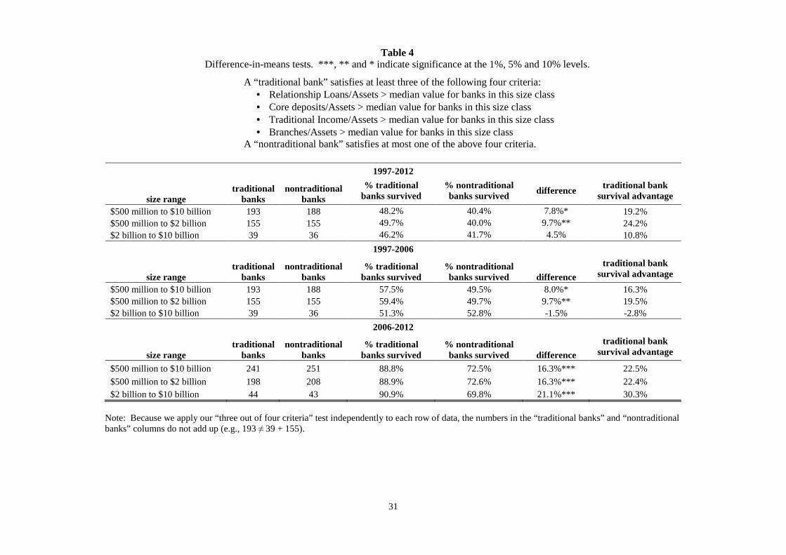
31

Table 4

Difference-in-means tests. ***, ** and * indicate significance at the 1%, 5% and 10% levels.

A “traditional bank” satisfies at least three of the following four criteria: • Relationship Loans/Assets > median value for banks in this size class • Core deposits/Assets > median value for banks in this size class • Traditional Income/Assets > median value for banks in this size class • Branches/Assets > median value for banks in this size class

A “nontraditional bank” satisfies at most one of the above four criteria.

1997-2012

size range traditional

banks nontraditional

banks

% traditional banks survived

% nontraditional banks survived

difference traditional bank

survival advantage

$500 million to $10 billion 193 188 48.2% 40.4% 7.8%* 19.2% $500 million to $2 billion 155 155 49.7% 40.0% 9.7%** 24.2% $2 billion to $10 billion 39 36 46.2% 41.7% 4.5% 10.8%

1997-2006

size range traditional

banks nontraditional

banks % traditional

banks survived % nontraditional banks survived difference

traditional bank survival advantage

$500 million to $10 billion 193 188 57.5% 49.5% 8.0%* 16.3% $500 million to $2 billion 155 155 59.4% 49.7% 9.7%** 19.5% $2 billion to $10 billion 39 36 51.3% 52.8% -1.5% -2.8%

2006-2012

size range traditional

banks nontraditional

banks % traditional

banks survived % nontraditional banks survived difference

traditional bank survival advantage

$500 million to $10 billion 241 251 88.8% 72.5% 16.3%*** 22.5%

$500 million to $2 billion 198 208 88.9% 72.6% 16.3%*** 22.4% $2 billion to $10 billion 44 43 90.9% 69.8% 21.1%*** 30.3%

Note: Because we apply our “three out of four criteria” test independently to each row of data, the numbers in the “traditional banks” and “nontraditional banks” columns do not add up (e.g., 193 ≠ 39 + 155).

32

Table 5 Cross-sectional probit model. Banks with assets between $500 million and $10 billion in 1997:

Probi(Survive until 2012) = a + b*Traditional Indexi,1997 + c*ECONi,1997-2012 + d*Zi,1997 + ei The even-numbered columns include a first-stage Heckman selection procedure (see Appendix). The cells display the estimated marginal probabilities. ***, ** and * indicate significance at the 1%, 5% and 10% levels.

[1] [2] [3] [4] [5] [6]

Traditional index 0.0063*** 0.0029** 0.0067*** 0.0028** 0.0052** 0.0049** (0.0021) (0.0021) (0.0021) (0.0022) (0.0024) (0.0024) State GDP -0.0342 -0.0131 (0.0238) (0.0163) State Unemployment -0.0354 -0.0162 (0.0271) (0.0169) State Credit Quality -0.7538*** -0.7228*** (0.0677) (0.1755) lnAssets -0.0206 -0.0061 -0.0151 -0.0031 -0.0033 -0.0026 (0.0331) (0.0203) (0.0330) (0.0184) (0.0353) (0.0341) Risk-weighted Assets -0.0107*** -0.0060*** -0.0112*** -0.0059*** -0.0089*** -0.0086*** (0.0024) (0.0033) (0.0025) (0.0034) (0.0031) (0.0036) Nonperforming Loans 0.0156 0.0147 0.0147 0.0137 0.0348 0.0348 (0.0306) (0.0170) (0.0303) (0.0159) (0.0336) (0.0348) Loan Concentration -0.3750*** -0.2177*** -0.3804*** -0.2075*** -0.5678*** -0.5447*** (0.1289) (0.1329) (0.1292) (0.1309) (0.1615) (0.1923) Commercial Real Estate Loans -0.0040 -0.0000 -0.0035 0.0003 -0.0036 -0.0032 (0.0034) (0.0022) (0.0034) (0.0020) (0.0043) (0.0043) Construction and Development Loans 0.0111 0.0063 0.0107 0.0059 0.0243*** 0.0233*** (0.0083) (0.0057) (0.0084) (0.0054) (0.0094) (0.0107) Goodwill 0.0122 0.0601** 0.0100 0.0593** 0.0856* 0.0916 (0.0440) (0.0284) (0.0444) (0.0275) (0.0509) (0.0828) Risk-based Capital 0.0239** 0.0024 0.0239** 0.0017 0.0315*** 0.0285** (0.0106) (0.0080) (0.0105) (0.0073) (0.0106) (0.0105) Funding Gap 0.0001*** 0.0001*** 0.0001*** 0.0001*** 0.0001*** 0.0001*** (0.0000) (0.0000) (0.0000) (0.0000) (0.0000) (0.0001) Noninterest Expense 0.0023 -0.0020 0.0019 -0.0022 0.0074** 0.0065 (0.0026) (0.0016) (0.0026) (0.0015) (0.0032) (0.0035) Return on Assets 0.0934* 0.0310 0.0849 0.0250 0.0645 0.0590 (0.0534) (0.0377) (0.0522) (0.0342) (0.0690) (0.0665) HHI 0.3689 0.0844 0.3497 0.0619 1.0297** 0.9725** (0.4607) (0.2864) (0.4679) (0.2724) (0.4366) (0.4487) Urban 0.0250 0.0008 0.0117 -0.0061 0.0634 0.0588 (0.1117) (0.0639) (0.1126) (0.0604) (0.1217) (0.1173) HHI*Urban -0.3035 -0.0487 -0.2901 -0.0240 -0.9042 -0.8478 (0.5534) (0.3289) (0.5612) (0.3139) (0.5633) (0.5503) Inverse Mills Ratio 0.3014*** 0.3111*** 0.0245 (0.1131) (0.1115) (0.1256) Heckman correction no yes no yes no yes N 541 541 541 541 531 531 pseudo R-sq 0.0674 0.0669 0.3294

33

Table 6 Panel probit model, 1997-2012. Banks with assets between $500 million and $10 billion:

Probi,t(Survive through year t) = a + b*Traditional Indexi,t-1 + c*Economic Conditionsi,t-1 + d*Zi,t-1 + τt + ei,t

Even-numbered columns include a first-stage Heckman selection procedure (see Appendix). All columns include year fixed effects. The cells display the estimated marginal probabilities. Standard errors are clustered at the bank level. ***, ** and * indicate significance at the 1%, 5% and 10% levels.

[1] [2] [3] [4] [5] [6] Traditional index 0.0006** 0.0012** 0.0006*** 0.0012** 0.0006** 0.0012** (0.0002) (0.0006) (0.0002) (0.0007) (0.0002) (0.0007) State GDP -0.0008 -0.0005 (0.0016) (0.0037) State Unemployment 0.0045 0.0113* (0.0028) (0.0080) State Credit Quality 0.0003 0.0007 (0.0036) (0.0083) lnAssets -0.0013 0.0019 -0.0017 (0.0013 -0.0004 0.0040 (0.0034) (0.0081) (0.0034) 0.0083) (0.0034) (0.0087) Risk-weighted Assets -0.0009*** -0.0024*** -0.0009*** -0.0026*** -0.0009*** -0.0026*** (0.0003) (0.0013) (0.0003) (0.0013) (0.0003) (0.0014) Nonperforming Loans -0.0056*** -0.0120** -0.0058*** -0.0130*** -0.0056** -0.0127** (0.0022) (0.0060) (0.0022) (0.0063) (0.0023) (0.0065) Loan Concentration -0.0447*** -0.1471*** -0.0457*** -0.1576*** -0.0458*** -0.1553*** (0.0169) (0.0844) (0.0170) (0.0880) (0.0172) (0.0870) Commercial Real Estate Loans 0.0002 0.0013 0.0001 0.0011 0.0003 0.0014 (0.0004) (0.0012) (0.0004) (0.0012) (0.0004) (0.0013) Construction and Development Loans 0.0006 0.0015 0.0006 0.0017 0.0006 0.0014 (0.0006) (0.0014) (0.0006) (0.0015) (0.0006) (0.0015) Goodwill -0.0045** -0.0040 -0.0044** -0.0036 -0.0044** -0.0035 (0.0020) (0.0048) (0.0020) (0.0051) (0.0020) (0.0052) Risk-based Capital 0.0062*** 0.0116*** 0.0062*** 0.0120*** 0.0065*** 0.0125*** (0.0015) (0.0042) (0.0015) (0.0043) (0.0015) (0.0044) Funding Gap 0.0000 0.0007 0.0001 0.0008 0.0000 0.0007 (0.0002) (0.0007) (0.0002) (0.0008) (0.0002) (0.0008) Noninterest Expense -0.0002 -0.0013* -0.0002 -0.0014* -0.0002 -0.0014* (0.0003) (0.0010) (0.0003) (0.0011) (0.0003) (0.0011) Return on Assets 0.0059** 0.0112* 0.0060** 0.0119* 0.0058** 0.0113 (0.0028) (0.0067) (0.0028) (0.0070) (0.0028) (0.0070) HHI -0.0242 -0.1085 -0.0193 -0.1027 -0.0223 -0.1090 (0.0520) (0.1290) (0.0511) (0.1280) (0.0539) (0.1352) Urban -0.0058 -0.0163 -0.0050 -0.0151 -0.0064 -0.0187 (0.0137) (0.0308) (0.0136) (0.0313) (0.0140) (0.0325) HHI*Urban -0.0321 -0.0255 -0.0377 -0.0370 -0.0380 -0.0369 (0.0696) (0.1532) (0.0687) (0.1559) (0.0708) (0.1609) Inverse Mills Ratio 0.0235** 0.0241** 0.0242** (0.0101) (0.0101) (0.0102) Heckman correction no yes no yes no yes Year fixed effects yes yes yes yes yes yes Number of banks/clusters 544 544 544 544 533 533 Number of observations 5,206 5,206 5,236 5,236 5,094 5,094 pseudo R-sq 0.0774 0.0761 0.0774

34

Table 7 Panel probit model, 1997-2012. Banks in various asset size subsamples:

Probi,t(Survive through year t) = a + b*Traditional Indexi,t-1 * Crisist + b2* Traditional Indexi,t-1*(1-Crisist) + c*Economic Conditionsi,t-1 + d*Zi,t-1 + ei,t

Crisis = 1 for 2008-2012 and = 0 otherwise. All columns include a first-stage Heckman selection procedure (see Appendix). The cells display the estimated marginal probabilities. Standard errors are clustered at the bank level. ***, ** and * indicate significance at the 1%, 5% and 10% levels.

[1] [2] [3] $500M to

$10B $500M to

$2B $2B to $10B

Traditional Index*Crisis 0.0014*** 0.0014*** 0.0008 0.0003 0.0003 0.0005

Traditional Index*(1-Crisis) 0.0007** 0.0009*** -0.0004 0.0003 0.0003 0.0006

State Credit Quality -0.0065** -0.0065** -0.0068 0.0028 0.0030 0.0081

lnAssets 0.0094** 0.0114* 0.0055 0.0048 0.0069 0.0145

Risk-weighted Assets -0.0010** -0.0014** 0.0009 0.0005 0.0006 0.0009

Nonperforming Loans -0.0104*** -0.0079** -0.0192* 0.0038 0.0036 0.0115

Loan Concentration -0.0529** -0.0512* -0.0593 0.0249 0.0290 0.0587

Commercial Real Estate Loans 0.0011** 0.0012* 0.0021* 0.0005 0.0006 0.0011

Construction and Development Loans 0.0010 0.0011 -0.0008 0.0007 0.0008 0.0013

Goodwill -0.0056 -0.0040 -0.0196* 0.0053 0.0048 0.0108

Risk-based Capital 0.0047*** 0.0049*** 0.0042 0.0011 0.0012 0.0030

Funding Gap 0.0001 0.0003 -0.0006 0.0003 0.0003 0.0006

Noninterest Expense -0.0006 -0.0006 -0.0006 0.0004 0.0004 0.0011

Return on Assets 0.0030 0.0020 0.0122 0.0042 0.0040 0.0203

HHI -0.0228 0.0276 -0.1719 0.0650 0.0785 0.1120

Urban -0.0037 0.0005 -0.0018 0.0161 0.0190 0.0346

HHI*Urban -0.0671 -0.1039 0.0050 0.0901 0.1044 0.2086

Inverse Mills Ratio 0.0243** 0.0331** 0.0067 0.0101 0.0135 0.0125

Heckman correction yes yes yes Year fixed effects no no no Number of banks/clusters 533 428 105 Number of observations 5,094 4,095 956 pseudo R-sq 0.0587 0.0614 0.0922

35

Table 8 Panel probit model, 1997-2012. Various specifications and bank asset size subsamples:

Probi,t(Survive through year t) = a + b*Traditional Indexi,t-1 + c*Economic Conditionsi,t-1 + d*Zi,t-1 + τt + ei,t

All columns include a first-stage Heckman selection procedure (see Appendix). The cells display the estimated marginal probabilities. Standard errors are clustered at the bank level. ***, ** and * indicate significance at the 1%, 5% and 10% levels.

[1] [2] [3] [4] [5] [6]

Bank Sizes $500M to $10B $500M to

$2B $2B to $10B

Traditional index 0.0013*** 0.0011*** 0.0014*** 0.0012** 0.0019** -0.0002 (0.0008) (0.0005) (0.0007) (0.0007) (0.0009) (0.0004) State Credit Quality -0.0204*** -0.0194** -0.0173*** 0.0007 -0.0036 0.0082 (0.0059) (0.0073) (0.0079) (0.0083) (0.0122) (0.0106) lnAssets 0.0067 -0.0035 0.0176*** 0.0040 -0.0036 -0.0107 (0.0071) (0.0064) (0.0109) (0.0087) (0.0164) (0.0106) Risk-weighted Assets -0.0019*** -0.0026*** -0.0051*** 0.0004 (0.0011) (0.0014) (0.0022) (0.0006) Nonperforming Loans -0.0030 -0.0127** -0.0109 -0.0093* (0.0039) (0.0065) (0.0070) (0.0075) Loan Concentration -0.0836** -0.1553*** -0.2438*** -0.0577* (0.0633) (0.0870) (0.1287) (0.0582) Commercial Real Estate Loans 0.0018** 0.0014 0.0030* 0.0005 (0.0013) (0.0013) (0.0023) (0.0010) Construction and Development Loans 0.0023** 0.0014 0.0018 -0.0004 (0.0015) (0.0015) (0.0022) (0.0010) Goodwill -0.0045 -0.0035 0.0020 -0.0070** (0.0038) (0.0052) (0.0097) (0.0042) Risk-based Capital 0.0125*** 0.0125*** 0.0178** 0.0033 (0.0047) (0.0044) (0.0059) (0.0030) Funding Gap 0.0002 0.0007 0.0020** -0.0002 (0.0005) (0.0008) (0.0014) (0.0003) Noninterest Expense -0.0004 -0.0014* -0.0023* -0.0009* (0.0007) (0.0011) (0.0017) (0.0009) Return on Assets 0.0071 0.0113 0.0163* 0.0016 (0.0054) (0.0070) (0.0092) (0.0081) HHI -0.0711 -0.1090 0.0386 -0.1065* (0.1163) (0.1352) (0.2626) (0.1059) Urban -0.0180 -0.0187 -0.0032 -0.0054 (0.0279) (0.0325) (0.0560) (0.0237) HHI*Urban -0.0473 -0.0369 -0.2081 -0.0001 (0.1343) (0.1609) (0.3055) (0.1206) Inverse Mills Ratio 0.0266*** 0.0268*** 0.0206 0.0242** 0.0329** 0.0069 (0.0095) (0.0092) (0.0109) (0.0102) (0.0135) (0.0127) Heckman correction yes yes yes yes yes yes Year fixed effects no yes no yes yes yes Number of banks/clusters 533 533 533 533 428 105 Number of observations 5,094 5,094 5,094 5,094 4,095 956

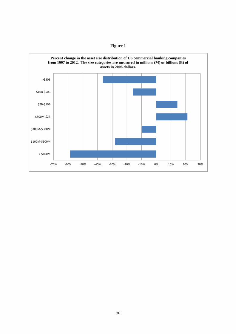
36

Figure 1

-70% -60% -50% -40% -30% -20% -10% 0% 10% 20% 30%

< $100M

$100M-$300M

$300M-$500M

$500M-$2B

$2B-$10B

$10B-$50B

>$50B

Percent change in the asset size distribution of US commercial banking companies from 1997 to 2012. The size categories are measured in millions (M) or billions (B) of

assets in 2006 dollars.

37

Appendix Table A1 Definitions and summary statistics for all variables in Tables 2 and 3. 546 observations of banks at year-end 1996.

Name Definition Mean Std. Dev. Min Max

Business Loans Commercial and industrial loans (not secured by real estate), as a percentage of total assets. 9.8 7.7 0.0 49.6 Household Loans Consumer loans, 1-4 family mortgage loans, and home equity loans, as a percentage of total

assets. 34.7 16.7 0.0 99.6

Relationship Loans Business Loans plus Household Loans. 44.5 14.2 7.1 99.6 Real Estate Loans Commercial real estate loans, construction and development loans, and nonfarm nonresidential

mortgages, as a percentage of total assets. 11.9 7.7 0.0 63.0

Total Loans Total loans divided by total assets. 62.5 13.0 14.0 99.6 Core Deposits Transactions deposits and small time deposits, as a percentage of total assets. 71.2 10.0 44.9 88.5 Noninterest Income Total noninterest income as a percentage of $1,000 of assets. 10.9 16.0 0.2 262.8 Traditional Fee Income Noninterest Income minus income from nontraditional financial services (e.g., investment

banking, securities brokerage, loan securitization and servicing, venture capital, insurance underwriting and sales, mutual fund sales), as a percentage of $1,000 of assets.

9.2 14.2 0.1 252.5

Traditional Income Traditional Fee Income plus net interest income (interest revenue minus interest expense minus provisions for loan losses), as a percentage of $1,000 of assets.

48.6 20.0 18.1 266.8

Branches Number of branches per $1,000 of assets. 0.02 0.01 0.0 0.07 Return on Assets Net income as a percentage of total assets. 1.1 0.4 -0.5 2.4 Noninterest Expense Noninterest expense as a percentage of operating income (interest income plus noninterest

income minus interest expense minus provisions for loan losses). 60.8 10.2 36.7 99.8

%Asset Growth, Previous 3 Years Percentage growth in total assets between 1994 and 1997. 61.0 62.3 -14.2 254.6 Tier 1 Risk-based Capital Ratio Tier 1 equity capital as a percentage of risk-weighted assets. 14.2 5.9 8.0 54.0 Risk-weighted Assets Risk-weighted assets as percentage of total assets. 64.3 12.8 25.6 171.3 Nonperforming Loans Loans 90 days past due plus nonaccrual loans, as a percentage of total assets. 0.6 0.8 0.0 11.5 Funding Gap Total loans as a percentage of total deposits. 75.8 16.9 25.2 114.4 Unused Loan Commitments and Lines Unused loan commitments as a percentage of total assets. 0.1 0.1 0.0 0.4 Liquid Assets Cash, interest-bearing cash, and securities, as a percentage of total liabilities. 25.4 12.4 3.2 71.8

38

Appendix Table A2 Definitions and summary statistics for all variables used in the estimates in Table 5. 541 observations of banks at year-end 1996.

Name Definition Mean Std. Dev. Min Max

Survive Equals one if bank survived from 1997 through 2012. 0.45 0.5 0.0 1.0 Traditional Index An index running from 0 (a fully nontraditional bank) to 100 (a fully traditional bank).

Additional details available in the text. 39.6 12.1 0.0 100.0

State GDP State-level average annual GDP growth rate for 1997-2012, minus US average annual GDP growth rate for 1997-2012, expressed as a percentage.1

-0.2 1.0 -3.0 3.6

State Unemployment State-level average annual unemployment rate for 1997-2012, minus US average annual unemployment rate for 1997-2012, expressed as a percentage.1

-0.1 0.9 -4.8 2.4

State Credit Quality State-level average annual nonperforming loan ratio for 1997-2012, minus US average annual nonperforming loan ratio 1997-2012, expressed as a percentage.1,2

-0.7 0.5 -2.7 1.2

lnAssets Total assets, in millions of 2006 dollars, expressed as natural log. 6.8 0.7 6.0 9.0 Risk-weighted Assets Risk-weighted assets as percentage of total assets. 64.3 12.9 25.6 171.3 Nonperforming Loans Loans 90 days past due plus nonaccrual loans, as percentage of total assets. 0.6 0.7 0.0 11.5 Loan Concentration Herfindahl index of loan portfolio shares (real estate loans, commercial and industrial loans,

agricultural loans, loans to depository institutions, loans to individuals, loans to foreigners). 0.6 0.2 0.3 1.0

Commercial Real Estate Loans Nonfarm nonresidential mortgage loans as percentage of total assets. 11.9 7.7 0.0 63.0 Construction Loans Constructions and development loans as percentage of total assets 3.0 3.0 0.0 23.0 Goodwill Goodwill, as percentage of total assets. 0.3 0.5 0.0 3.4 Risk-based Capital Tier 1 equity capital as a percentage of risk-weighted assets. 9.0 2.7 5.1 33.1 Funding Gap Total loans as a percentage of total deposits. 75.8 16.9 25.2 114.4 Noninterest Expense Noninterest expense as a percentage of operating income (interest income plus noninterest

income minus interest expense minus provisions for loan losses). 60.7 11.2 16.4 133.9

Return on Assets Net income as a percentage of total assets 1.1 0.6 -5.7 5.2 HHI County deposit share Herfindahl index.3 0.2 0.1 0.0 0.7 Urban Equals 1 if the bank is headquartered in a Metropolitan Statistical Area (MSA) 0.8 0.4 0.0 1.0

1 When a bank operates in more than one state, we construct a multistate average, using the proportions of the bank’s deposits in each state as weights. 2 We calculate the state-level average nonperforming loan ratios using data only from banks that get at least 75% of their deposits from within the state. 3 When a bank operates in more than one county, we construct a multicounty average, using the proportions of the bank’s deposits in each county as weights.

39

Appendix Table A3

First-stage Heckman estimations. Probit estimation for the probability of selection into the second stage sample. ***, ** and * indicate significance at the 1%, 5% and 10% levels.

Cross-section Panel Risk-based Capital -0.01013*** -0.00315*** (0.00124) (0.00092) Funding Gap 0.00037 0.00128*** (0.00024) (0.00019) Risk-weighted Assets -0.00029 -0.00093** (0.00039) (0.00036) Return on Assets -0.01416 -0.00454* (0.01026) (0.00273) Loan Concentration -0.04369** -0.08341*** (0.02087) (0.01780) Commercial Real Estate Loans 0.00201*** 0.00085*** (0.00043) (0.00031) Noninterest Expense -0.00295*** -0.00150*** (0.00037) (0.00022) Goodwill 0.04420*** 0.01767*** (0.00589) (0.00186) ln(Population) 0.00697** 0.00985*** (0.00350) (0.00317) ln(Per Capita GDP) 0.18107*** 0.12663*** (0.02412) (0.02030) Age -0.00022*** -0.00039*** (0.00008) (0.00008) N 6,861 79,641

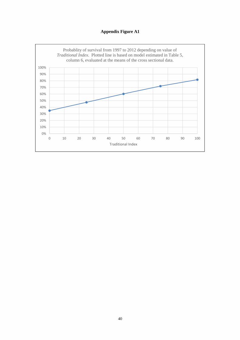
40

Appendix Figure A1

0%

10%

20%

30%

40%

50%

60%

70%

80%

90%

100%

0 10 20 30 40 50 60 70 80 90 100

Traditional Index

Probablity of survival from 1997 to 2012 depending on value of Traditional Index. Plotted line is based on model estimated in Table 5,

column 6, evaluated at the means of the cross sectional data.

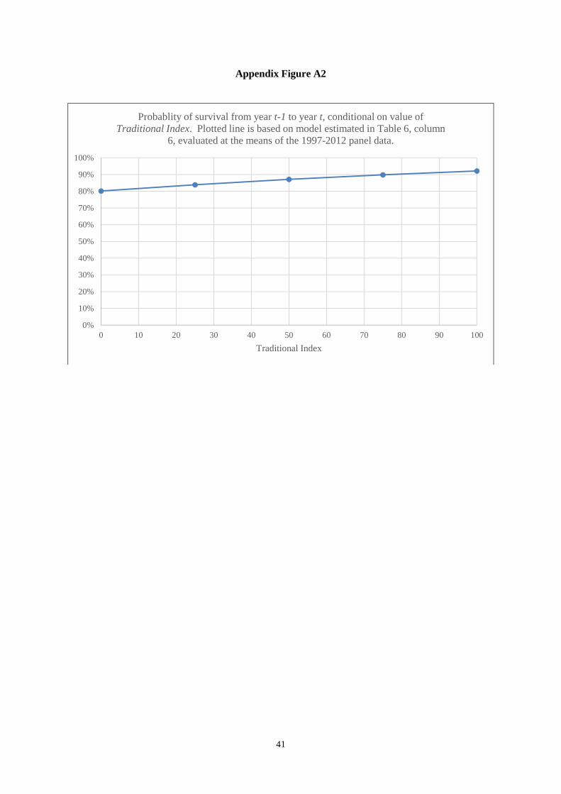
41

Appendix Figure A2

0%

10%

20%

30%

40%

50%

60%

70%

80%

90%

100%

0 10 20 30 40 50 60 70 80 90 100

Traditional Index

Probablity of survival from year t-1 to year t, conditional on value of Traditional Index. Plotted line is based on model estimated in Table 6, column

6, evaluated at the means of the 1997-2012 panel data.

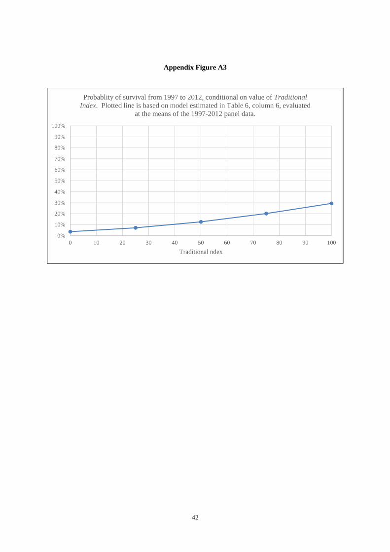
42

Appendix Figure A3

0%

10%

20%

30%

40%

50%

60%

70%

80%

90%

100%

0 10 20 30 40 50 60 70 80 90 100

Traditional ndex

Probablity of survival from 1997 to 2012, conditional on value of Traditional Index. Plotted line is based on model estimated in Table 6, column 6, evaluated

at the means of the 1997-2012 panel data.