Is the Original Taylor Rule Enough? Simple versus Optimal ... · Is the Original Taylor Rule...

Is the Original Taylor Rule Enough? Simple versus Optimal Rules as Guides to Monetary Policy

William A. Brock, Steven N. Durlauf, James M. Nason, and Giacomo Rondina1

November 1, 2006

Conference Version: Preliminary and Incomplete

1University of Wisconsin, University of Wisconsin, Federal Reserve Bank of Atlanta, and University of Wisconsin respectively. The views herein represent those of the authors and are not those of either the Federal Reserve Bank of Atlanta, the Federal Reserve System, or any of its staff.

“..hold your tongue, I charge you, for the case is manifest…Did I not charge you not to speak? ‘twas plain enough before; and now you have puzzled it again.”

Gripus, the Theban Judge Amphitryon, John Dryden

1. Introduction

This paper contributes to the monetary policy evaluation literature by developing

new strategies to study a few alternative policy rules that are the core of recent research.

We are interested in assessing the case that can be made for optimal rules as opposed to

simple rules for monetary policy. In our context, an optimal rule represents the solution

to an intertemporal optimization problem in which a loss function for the policymaker

and an explicit model of the macroeconomy are specified. By a simple rule, we refer to

heuristics that embody the intuitions policymakers and economists have about how a

central bank should react to aggregate disturbances. The classic example of a simple

heuristic is Friedman’s k% money growth rule.

Modern versions of simple monetary policy rules typically embody a notion of

“leaning against the wind”.2 In this case, a central bank plays an active role in stabilizing

macroeconomic aggregates. The canonical modern example of a simple policy heuristic

is Taylor’s rule (1993), in which the Federal funds rate is increased in response to output

relative to trend and by more than one-for-one with the inflation rate. Taylor’s rule is

motivated by the notion that a central bank should attempt to reverse aggregate demand

shocks, whereas aggregate supply shocks should be allowed to work unhindered in the

economy.

The distinction between optimal and simple rules has taken on particular

significance in recent debates over the desirability of inflation targeting, as exemplified in

the competing views expressed in Svensson (2003) and McCallum and Nelson (2005).

The latter paper takes particular interest in the claim made by Svensson that inflation

targeting rules are preferable to instrument rules because they can embody the restrictions

2Tobin (1983) distinguishes between fixed and reactive rules. Modern work focuses on the latter.

1

intertemporal optimality places on the solution to the optimal policy problem.3 As a

theoretical matter, McCallum has shown that in principle an instrument rule may

arbitrarily well approximate a targeting rule, so long as the same information set is

available for conditioning. Nonetheless, Svensson’s claim has force when targeting rules

are compared to simple rules of the type in which we are interested.4

In this paper, we question the case for optimal rules at two levels. First, we

consider the role model uncertainty plays in vitiating the superiority of optimal to simple

rules. As argued by McCallum and Nelson (2005)5, the optimality of a rule with respect

to a given economic environment begs the question of its evaluation when the true model

of the economy is not known. Our paper evaluates this issue by comparing the original

Taylor rule with a model-specific optimal interest rule in the presence of various types of

model uncertainty. Second, we compare simple and optimal rules from the perspective of

what we call preference uncertainty. By preference uncertainty, we refer to uncertainty

about the assumption that the objective function of a policymaker only depends on the

variances of various states and controls. Our specific objective is to compare rules with

respect to their effects on the variance of states at different frequencies. When a

policymaker associates different losses to fluctuations at different frequencies, an analyst

faces uncertainty as to which frequencies matter.

The analyst needs to study how rules drive fluctuations in various macroeconomic

aggregates frequency by frequency to understand the role preference uncertainty plays in

policymaking. Conventional policy assessments assume that the preferences of the

policymaker are summarized by the variances of the aggregates under study. As we

discuss below, such preferences ignore the disparate short-, medium- and long-run affects

of policy. Since Brock and Durlauf (2004,2005) and Brock, Durlauf, and Rondina (2006)

show that the choice of a policy rule yields a frequency by frequency variance tradeoff,

3Some of the arguments that appear in the literature strike us as self-evidently weak; for example, the claim that a targeting rule uses the entire information set of the policymaker. It is obvious that any information available for a targeting rule may be exploited by an instrument rule. 4Notice that the comparison of targeting rules to simple instrument rules renders moot the claim that targeting rules are more transparent than instrument rules. 5See McCallum (1988,1999) for early discussions of model uncertainty and monetary policy that broadly study many of the questions we wish to consider.

2

we argue that these tradeoffs should be reported to a policymaker, to account for different

preferences with respect to fluctuations at different cycles. We wish to be clear that when

we refer to preference uncertainty, we do not mean that the central bank does not know

its own preferences. Rather, we believe it is important to report information on policy

comparisons that avoid assuming a particular loss function for the central bank. For our

purposes, this means that we wish to draw comparisons that reflect the possibility that the

policymaker cares about fluctuations at some cycles more than others.

Our focus will be on monetary policy environments in which one engages in a

binary comparison between a simple rule and a model-specific optimal alternative. Why

focus on such stark comparisons between simple and optimal rules? We believe this

exercise is useful in understanding how strong the case is for optimal approaches to

monetary policy. The exercise matters because this is the decision problem a central

bank must address when choosing one rule over another. We do not claim that our

analysis proves either that the simple rules are superior to model-specific optimal rules in

general or that the Taylor rule is superior to an inflation targeting rule in particular.

Rather, we want to evaluate the strength of support in favor of optimal rules when

compared to a standard rule of thumb for monetary policy; unlike Dryden’s judge we

think it important to understand when a case is not settled. Our conclusion is that there

are not compelling reasons to favor an optimal rule over a rule of thumb, at least for the

contexts we study.

As such, our analysis is in the spirit of Friedman (1948) whose conceptualization

of a framework in which money growth is constant is very much couched in an explicit

consideration of the information limits faced by a central bank. Friedman concludes his

classic paper with (pg. 263)

…I should like to emphasize the modest aim of the proposal. It does not claim to provide full employment…It does not claim to eliminate entirely cyclical fluctuations in output and employment. Its claim to serious consideration is that it provides a stable framework of fiscal and monetary action, that it largely eliminates the uncertainty…of discretionary actions by government authorities…It is not perhaps a proposal that one would consider at all optimum if our knowledge of the fundamental causes of cyclical fluctuations were considerably greater than I think them to be; it is a proposal that involves minimum reliance on uncertain and untested knowledge.

3

Model uncertainty has, due to the pioneering work of Hansen and Sargent ((2003)

and especially (2006)) on robustness, become a major feature of current research.6 In this

paper we follow an approach developed in Levin and Williams (2003) and Brock,

Durlauf, and West (2003, 2006) to evaluate policies in the presence of model uncertainty.

The idea of this approach is to first construct a model space that includes all candidate

models for the economy, evaluate policies for each of the candidate models, and then

determine how to draw policy influences given the fact that the true model is unknown.

This approach differs from the usual robustness analysis in that we do not focus on model

misspecification which is measured local to a given baseline model.

Given a model space, it is necessary to determine how to aggregate information

on rule performance across the different models. In this paper, we consider non-Bayesian

approaches that are based on minimax and minimax regret criteria. These approaches

involve guarding against “worst case scenarios”, but do so in different ways that we

formalize below. Relative to the Bayesian approach described below, neither minimax

nor minimax regret requires the policymaker to take a stance on model space priors in

order to compute posterior model probabilities.

Our analysis does not address the question of the design of optimal rules in the

presence of model uncertainty. We regard this as an important, but distinct question from

understanding the sensitivity of rules to model uncertainty. We believe our exercise is

useful because it provides insights into how to evaluate the performance of rules in the

presence of model uncertainty that cannot be explicitly described in advance. There are

fundamental conceptual questions involved in thinking about policy effects when one

cannot specify the support of the uncertainty faced by a policymaker. Nevertheless, we

believe insights into this difficult problem are found from understanding how rules

perform within a model space when, by construction, the rules fail to account for model

uncertainty. Our approach to non-Bayesian decision theory follows Hansen and Sargent

(who focus on minimax evaluation). Since we operate within somewhat different model

spaces, it requires additional justification for our approach.

6Examples that focus on monetary policy include Giannoni (2002), Onatski and Stock (2002) and Tetlow and von zur Muehlen (2001).

4

We follow Levin in Williams (2003) in placing primary focus on model

uncertainty with respect to forward- and backwards-looking elements to inflation. In the

context of the Phillips curve, the 2005 special issue, “The econometrics of the New

Keynesian price equation”, in the Journal of Monetary Economics reveals little

consensus about the response of inflation to forward- and backward-looking expectations.

In that issue, the Rudd and Whelan paper is especially clear about how disagreements

over inflation dynamics create uncertainty for new Keynesian model building.

Section 2 describes our basic framework for assessing model uncertainty. Section

3 discusses the evaluation of frequency-specific effects of policies. Section 4 analyzes

some standard single input single output systems. Section 5 considers a standard two

equation IS/PC model and focuses on comparing Taylor’s original rule with a model- and

preference-specific optimal alternative. Section 6 provides summary and discussion of

future research directions.

2. Model uncertainty: basic ideas

At an abstract level, the issue of model uncertainty is easily described. Suppose

that a policymaker is choosing from a set P of alternative policies. Given , which

captures whatever features of the economy matter to the policymaker, a policymaker

experiences a loss associated with those features

Θ

( ).l Θ (1)

The features defined by Θ are not, for interesting cases, a deterministic function of a

policy and so are in general described by a conditional probability

( ), ,p d mµ Θ (2)

5

where we explicitly allow the state of the economy to depend on the policy choice, p ,

the available data, d, and the model of the economy that is assumed to apply, m. Data

dependence in this conditional probability may incorporate both direct dependence, as

occurs in an autoregression, where forecasts depend on past realizations, or uncertainty

about parameters. For simplicity, we measure losses as positive, so a policymaker

wishes to minimize (1) by choosing a policy to affect (2). Our goal in the analysis is to

relax the assumption that the policymaker knows the correct model of the economy, m.

Rather, we assume that the policymaker knows that the correct model lies in a model

space M. This space reflects uncertainty about the appropriate theoretical and functional

form commitments needed to allow quantitative analysis of the effects of a policy.

Why treat model dependence explicitly in this formulation while subsuming other

sources of uncertainty about ? Hansen and Sargent (2006) provide an extensive

discussion of these and other issues; see also Brock, Durlauf, West (2003). We see two

arguments as particularly important. One has to do with preferences: there are reasons to

believe that individual preferences may treat model uncertainty differently from other

types of uncertainty. These arguments are often based on experimental evidence of the

type associated with the Ellsberg paradox, in which individuals appear to evaluate model

uncertainty differently from other types. Put differently, the experimental evidence

suggests that preferences exhibit ambiguity aversion as well as risk aversion, when model

uncertainty is considered. For our purposes, what matters is that the evidence of

ambiguity aversion suggests a tendency to guard against the worst case scenario with

respect to models. A second justification concerns the levels at which model uncertainty

occurs. As discussed in Brock, Durlauf, and West (2003,2006), model uncertainty exists

at different levels: theory uncertainty, specification uncertainty, and parameter

uncertainty. These different levels may have different salience; for example we do not

think there is good evidence that parameter uncertainty within tightly specified models is

as important a source of model uncertainty as differences in theoretical commitments to

the presence of forward- and backward-looking elements in the Phillips curve. These

differences are best accommodated by treating model uncertainty as distinct from data

dependence.

Θ

6

The distinction between model uncertainty and other types of uncertainty is not

unambiguous. For example, it is often the case that models may be nested, so that a

given model may differ from another because a coefficient is zero. To be concrete, one

can nest a finite model space which contains a pure backward-looking and pure forward-

looking Phillips curve by considering a model space which contains a continuum of

models which consist of weighted averages of the models. Any analysis of model

uncertainty necessarily depends on prior judgments as to what models are of interest.

In this paper we focus on non-Bayesian decision criteria with respect to model

uncertainty. In order to understand why we take this route, recall that the standard

Bayesian solution to the optimal policy problem solves

( )( ) ( )( ) ( )min , , , ,p Pm M

E l p d M E l p d m m dµ∈∈

Θ = Θ∑ (3)

where (m dµ ) denotes the posterior probability that model m is the correct one.7,8

Recalling that

( ) ( ) ( )d m m d mµ µ µ∝ (4)

the Bayesian approach thus requires explicit assignment of model priors. The

assignment of these priors is problematic since a researcher rarely possesses any

meaningful prior knowledge from which priors may be constructed. The default prior in

the model uncertainty literature assigns equal probabilities to all elements of the model

space; but as discussed in Brock, Durlauf, and West (2003) such an approach is hard to

justify. Hence, a first limitation of Bayesian approaches to model uncertainty is the

requirement of introducing priors that have little meaning. There has been work on

7We do not address the issue of how to interpret these probabilities when none of the models is true. This is a deep and unresolved problem; see Key, Perrichi and Smith (1998) for some efforts to address. 8The Bayesian solution to model uncertainty involved model averaging, an idea suggested in Leamer (1978) and developed in detail in the work of Adrian Raftery, e.g. Raftery, Madigan, and Hoeting (1997).

7

evaluating the robustness of Bayesian inferences to prior choice in the statistics literature

as well as efforts in the econometrics literature to develop alternatives to the diffuse

priors that are used in the model uncertainty literature, but neither of these approaches is

well understood for the context we study. We should note that the problem of defining

priors continues to be a barrier to the adoption of Bayesian methods; Freedman (1991) is

an example of a major statistician who has rejected Bayesianism for this reason.

Beyond the issue of priors, we feel that there are other good reasons, for at least

some exercises, to avoid weighting models by posterior weights. These have to do with

the interpretation of the likelihood component in (4), i.e. ( )m dµ . In our judgment, the

utility of models is context dependent. A model which fits the overall data well, i.e.

receives a high value of (m dµ ) , may perform relatively poorly when employed to

consider regime changes when compared to another model whose overall fit is poorer. It

is easy to see how this could be the case when the model which fits historical data less

well is relatively immune to the Lucas critique.

Finally, it is important to recognize that the model spaces studied in

contemporaneous macroeconomics have not arisen sui generis; they reflect a history of

data work and as such, their relative fits reflect the evolution of empirical work so that

one type of model may be evolved to achieve better fit than another because of data

mining reasons. In this sense, one should not reify a model space as representing the

unique set of candidate models that were available to a researcher prior to data analysis.

This is not to say that model spaces do not reflect prior theoretical differences of course;

rather that the econometric versions of models that are under consideration at a point in

time have been influenced by the path of empirical work.

Non-Bayesian methods attempt to avoid dependence of inferences on model

probabilities, typically by looking for extremes in behavior. At an intuitive level, these

approaches abandon the search for optimal rules (in the Bayesian decision theory sense)

in favor of good rules, where good is equated with the notion that the rule works

relatively well regardless of which model is true. The minimax approach, proposed by

Wald (1950), chooses a policy so that the loss under it is minimized under the least

8

favorable model (relative to that rule) in the model set. Formally the minimax policy

choice is

( )( )min max , ,p P m M E l p d m∈ ∈ Θ . (5)

This formulation has been pioneered by Hansen and Sargent for macroeconomic contexts

and forms the basis of the literature on robustness analysis. From the perspective of the

economic theory literature, versions of minimax have been justified by Gilboa and

Schmeidler (1989) among others. This type of work has in fact suggested that in addition

to risk aversion (which leads to Bayesian expected loss calculations) agents can also

exhibit ambiguity aversion, which applies to environments where probabilities cannot be

assigned to possible outcomes (in our case models). The ambiguity aversion literature

provides axiomatic justifications for minimax. Some of these, e.g. Epstein and Wang

(1994), suggest that policies should be evaluated based on a weighted combination of

losses under the least favorable model and the expected loss across models, an idea

originally due to Hurwicz (1951); this is done in Brock, Durlauf, and West (2003), but we

do not do so here given our desire not to assign model probabilities.

A standard criticism of the minimax criterion is that it is inappropriately

conservative as it assumes the worst case possible in assessing policies. The force of this

criticism, in our view, depends on whether the policy choice is driven by a relatively

implausible model. This of course leads back to the question of model probabilities, the

reasons for eschewing we have already given. As it turns out, there is an alternative non-

Bayesian approach which moves away from the idea that the worst outcome should

always be assumed: minimax regret. Minimax regret was originally proposed by Savage

(1951) explicitly in order to avoid the pessimism of minimax. This approach focuses on

the comparison of the effects of a given policy with the optimal one given knowledge of

the true model. For a given policy p and model m, regret ( ), ,R p d m is defined as

( ) ( )( ) ( )( ), , , , min , ,p PR p d m E l p d m E l p d m∈= Θ − Θ . (6)

9

In words, the regret associated with a policy and model measures the loss incurred by the

policy relative to what would have been incurred had the optimal policy been based upon

the model. The minimax regret policy is correspondingly defined by

( )min max , ,p P m M R p d m∈ ∈ . (7)

When there are only two policies 1p and 2p under consideration, it is convenient to work

with measures of maximum regret MR

( ) ( )( ) ( )( )1 1max , , min , ,m M m M 2MR p E l p d m E l p d m∈ ∈= Θ − Θ (8)

and

( ) ( )( ) ( )( )2 2max , , min , ,m M m M 1MR p E l p d m E l p d m∈ ∈= Θ − Θ . (9)

Brock (2006) and Manski (2006) show that the minimax regret problem can be written as

[ ]

( ) ( ) ( ){ }10,1min , 1 2MR p MR pδ

δ δ∈

− . (10)

They further show that the optimal choice of δ is

( )( ) ( )

2

1 2

MR pMR p MR p

δ =+

. (11)

Notice that the weighting parameter δ , which will represent how one should weight the

two candidate policies when making a policy choice, will depend smoothly on the

maximum regret values; as such minimax regret avoids the property of minimax analysis

that small changes in the payoffs of policies can lead to discontinous changes in the

optimal policy choice.

10

Primarily due to seminal papers by Manski (2005,2006)9, minimax regret has

recently received a great deal of attention in the microeconometrics literature; but as far

as we know it has not been used to study macroeconomic questions in general, let alone

with respect to questions associated with policy evaluation.

One objection to the minimax regret criterion is that decisionmaking under it is

not required to obey the axiom of independence of irrelevant alternatives (IIA),

something first shown in Chernoff (1954). It is not clear that this axiom is appropriate

for policy decisions, as opposed to individual ones. Without focusing on the

individual/policymaker distinction, we can see reasons why the axiom may not be

natural. The axiom in essence states that one’s preferences over different pairs of actions

does not depend on the context in which they are made, where the total choice set is part

of the context. This is not an obvious requirement of rationality.10 In absence of the

axiom, there do exist coherent axiom systems that produce minimax regret as the

standard for evaluation; Stoye (2006) is the state of the art treatment. Further, we would

note that there are many results in the behavioral economics literature that speak against

the axiom; indeed, as discussed in Camerer and Loewenstein (2003), what are known as

context effects in behavioral economics directly challenge the IIA assumption.

We do not predicate our interest in minimax regret on a strong adherence to any

of these arguments against the IIA assumption. For our purposes, we follow Manski and

use minimax as a way of understanding policy effects without insisting on the superiority

of minimax or any other decision rule.

A second issue that arises in our calculations concerns the role of randomized

strategies as candidates for central bank policy. In our analysis, we will have recourse to

allow for randomization between the Taylor rule and its model-specific optimal

9Chamberlain (2001) is an important precursor in suggesting minimax regret as an approach. 10Blume, Easley, and Halperin (2006) argue, for example, that an appropriate axiomatization of rationality should not require that agents have preferences which obey certain consistency conditions over all possible states of the world, as is required by Savage, but rather that rationality requires certain consistency conditions only over states under consideration. While they do not pursue this approach as a critique of irrelevance of independent alternatives, their work can be used to justify its exclusion as a rationality requirement.

11

counterpart. This is a corollary of our desire to treat the comparison between the two

rules as a decision problem and to use minimax regret for assessment: minimax regret

solutions can involve randomized strategies. Notice that to the extent that we conclude

that the case for an optimal rule over original Taylor rule is weak i.e. that the weight

placed on the Taylor rule is relatively large, it is a fortiori the case that the evidence

would be even weaker if other rules were added to the choice set facing the policymaker.

In this application we treat a minimax regret policymaker as using the fractions

suggested by the minimax regret calculation as weights to put on each rule, i.e. we posit

here that a central bank simply uses the minimax regret calculation as an heuristic device

to “hedge its bets” by choosing its policy to be the mix (suggested by the minimax regret

calculation) of the two under consideration. Thus, our suggested implementation of

minimax regret does not subject the public to the vagaries of the Federal Reserve flipping

a biased coin and choosing interest rate policy at random at each FOMC meeting. It is of

interest to ask what level welfare will actually be produced by using a mix of two policies

with positive weights. If welfare is concave in the policies, then the mixed policy assures

the policymaker that it will get at least as much welfare as a random policy. In our

exercises for backwards looking models, the maximization objective is concave and the

constraints are linear, so the welfare will indeed be concave in the policies. That said, we

are using the minimax regret weights as measures of support for the two policies, not for

randomization.

3. Frequency-specific effects of policies

As described above, we are also interested in understanding rule performance

with respect to fluctuations at different frequencies. Standard analyses of the effects of

policies focus on weighted averages of the unconditional variances of the states and

possibly controls. Hence, it is common to compare policies by considering, for example,

a weighted average of the unconditional variances of inflation and unemployment. Such

calculations thus mask the effects of policies on the variance of fluctuations at different

frequencies. Put differently, since the variance of a time series is the integral of its

12

spectral density, analyses of the integral will mask the effects of a policy on fluctuations

at different frequencies.

As a positive matter, these frequency-specific effects are of interest. As argued

in Brock and Durlauf (2004,2005) and Brock, Durlauf, and Rondina (2006), there can

exist fundamental tradeoffs in the variance associated with different frequencies of state

variables. Brock, Durlauf, and Rondina (2006) provide a general formal treatment. For

our purposes, it is sufficient to note that (abstracting away from issues of unit and

explosive roots), one can always interpret the effect of a feedback control rule

( ) 1tu L xπ t−= (12)

on the bivariate dynamical system

( ) ( ) ( )0 1t t t t t tA x E x A L x B L u W Lβ ε+= + + + (13)

in the following way. Let NCtx denote the system when 0tu ≡ , i.e. there is no control;

( )NCxf ω is the associated spectral density matrix.11 Each choice of control produces a

sensitivity function ( )CS ω such that

( ) ( ) ( ) ( )C C NC Cx xf S f Sω ω ω ω ′= . (14)

Different choices of the feedback rule thus shape the spectral density of the state

variables relative to the no control baseline. Hence, one can characterize what feedback

rules can achieve in terms of frequency-by-frequency effects on the state by

characterizing the set of sensitivity functions that are available to the policymaker. This

is the key idea underlying the notion of design limits to policy choice.

11When the uncontrolled system contains explosive or unit roots in the AR component, then the spectral density will not exist. Our formal results on restrictions on the sensitivity function still hold in this case. Our use of the spectral density of the uncontrolled system is done for heuristic purposes.

13

As shown in Brock, Durlauf, and Rondina (2006), for bivariate systems there is

a simple way to characterize the set of feasible sensitivity functions. For each

specification of a model of the uncontrolled system M and a control C, it must be the case

that the associated sensitivity function obeys

( )( ) (2

log det ,iS e d K M Cπ

ω

πω−

−=∫ ) . (15)

Brock, Durlauf, and Rondina show that whenever the system has no forward-looking

elements, i.e. 0β ≡ , the constraint will only depend on the unstable

autoregressive roots of the unconstrained system; the constraint will equal 0 if there are

no such roots, and is positive otherwise. This means that it is impossible to induce

uniform reductions in the spectral density matrix of the no control system, i.e. reductions

at some frequencies require increases at others. Of course, the overall variance may be

reduced. For forward-looking systems, the results are more complicated. It may be

possible to reduce the variance at all frequencies; nevertheless different rules still induce

different tradeoffs. Brock, Durlauf and Rondina show that a variance minimizing rule

may be one that increases the variance at some frequencies, even when a uniform

reduction is possible.

( ,K M C )

As a normative matter, should a central bank evaluate rules on the basis of

frequency specific effects? One reason, which is discussed in Onatski and Williams

(2003) and which we pursue in Brock, Durlauf, Nason, and Rondina (2006) with respect

to the effects on policy evaluation of alternative detrending methods, concerns the

problem of measuring low frequency components of state variables. Low frequency

behavior is of course hard to measure. Such measurement limitations take on particular

importance if it is believed that long-run movements in the data are those outside the

control of the central bank. For these reasons, it may seem reasonable for a policymaker

14

to compare the behavior of rules over integrals of “trimmed spectral densities,” i.e.

integrating spectral densities between [ ] [ ], ,π ς ς π− − ∪ rather than [ ],π π− .12

A second argument for considering frequency specific effects is based on the

nonseparable preferences. Under nonseparable preferences by a policymaker, different

weights are assigned to different frequencies in computing expected welfare; Otrok

(2001) has a nice example where the weights on different frequencies can differ by more

than 9:1. An important insight of Otrok is that if preferences exhibit habit persistence,

this means that the loss associated with volatility at high frequencies is greater than the

loss associated with volatility at low frequencies. This type of reasoning suggests that it

is important to consider how policies affect spectral densities over different intervals.

The upshot of this discussion is that we believe part of the communication

exercise for policymakers should involve reporting frequency specific comparisons.

4. Model uncertainty and monetary policy evaluation: basic ideas

a. parameter uncertainty

In this section we illustrate our suggestions on how to compare simple and

optimal policies in the context of a very stylized model consisting of a single state tx

described by

1t t tx ax u tε−= + + (16)

with associated control which obeys a feedback rule of the form tu

1tu fxt−= − . (17)

12Note that we are referring to integration of the spectral density in computing losses, not to the data per se. So this argument does not constitute a justification for the Hodrick-Prescott filter.

15

The policymaker’s objective is to compare two candidate feedback rules, i.e. the

policymaker can choose his actions from the action space { }1 2,f a a∈ . The model space

is

[ ]: ,M a a a∈ . (18)

We take the density aµ to be symmetric on support [ , ]a a . We assume that

1 2a aa a a a2+

< < << . (19)

Suppose that the objective function of the policymaker is to minimize the unconditional

variance of the state variable; for each model the loss function is therefore ( )2 | ,tE x f m .

Note that the control is costless in that its variance does not enter the loss function.

How do the different decision rules solve this problem? When policies are

evaluated using expected losses, the policy problem is

{ } ( ) { }1 2 1 2

2 2

, ,21 1min min log log

2 1 11

a

af a a f a aa

a f a fda f a fa f

ε εσ σµ∈ ∈

⎛ ⎞⎛ ⎞ ⎛+ − + −= −⎜ ⎟⎜ ⎟ ⎜− + − +− − ⎝ ⎠ ⎝⎝ ⎠

∫⎞⎟⎠

(20)

so long as neither of the policies produces a unit or explosive root in tx .

The minimax problem for the policymaker is

{ } ( )1 2

2

[ , ], 2min max1a a af a a a f

εσ∈∈

⎛ ⎞⎜⎜ − −⎝ ⎠

⎟⎟

(21)

which leads to the feedback rule

16

1

2 1

a a a af

a a a a1 2

2

aa

+ < +⎧= ⎨ + > +⎩

if if

(22)

independent of the relative plausibility of models in the model space. The behavior of the

policymaker is controlled by the boundaries of the space; a finding discussed in a similar

special case by Svensson (2002) and shown to hold for a general class of problems (when

the model space is local) by Brock and Durlauf (2005).

Finally, to calculate the minimax regret solution, one first calculates the expression

for maximum regret for each action, which are

( ) [ ] ( ) [ ] ( )

( )( )( )

1 , ,2 21

21

2 21 1

1 1max min1 1

1 11 1

a a a a a aMR aa a a a

a aa a a a

∈ ∈

⎛ ⎞ ⎛= −⎜ ⎟ ⎜

⎜ ⎟ ⎜− − − −⎝ ⎠ ⎝

−− =

− − − −

2

⎞=⎟

⎟⎠ (23)

and

( ) [ ] ( ) [ ] ( )

( )( )( )

2 , ,2 22

22

2 22 2

1 1max min1 1

1 1 .1 1

a a a a a aMR aa a a a

a aa a a a

∈ ∈

⎛ ⎞ ⎛= −⎜ ⎟ ⎜

⎜ ⎟ ⎜− − − −⎝ ⎠ ⎝

−− =

− − − −

1

⎞=⎟

⎟⎠ (24)

In both cases the minimum loss under the alternative policy is always equal to the

minimum loss reachable which is 1. The loss increases as the absolute distance between

the action and the model ia a− is increased.

In contrast to the minimax case, under minimax regret the policymaker can

optimally choose to play mixed strategies. Following the discussion in section 2, the

optimal minimax regret rule computes ( ) ( ) ( )( )1 2min , 1MR a MR aδ δ− where

17

( ) ( )( )

( ) ( )( ) ( ) ( )( )2 2

2 1

2 2 22 1 1 2

1

1 1

a a a a

a a a a a a a aδ

− − −=

− − − + − − − 2. (25)

Notice that the magnitude of this probability is sensitive to all combinations of feedback

parameters and and endpoints of the support of the autoregressive part of the state, 1a 2a

a and a . This is because, given a model, each rule is assessed according to how it

performs versus its alternative. This leads to the important difference between an optimal

policy under minimax regret compared to that under minimax: the continuity of δ with

respect to the change in the model space parameters a and a .

We can now relate this discussion to the comparison of a model specific optimal

policy and a rule of thumb. Let be the rule of thumb parameter and 1a 2 2a aa +

= so

that it represents the optimal feedback rule for (16).13 Our notion of the rule of thumb is

that the policymaker has some baseline feedback parameter that it wishes to consider as

opposed to the optimal feedback rule. As such the rule of thumb is in the spirit of the

original Taylor rule.

The minimax evaluation of the two rules yields a feedback parameter choice of

the form

1 1

1

2

2 2

a aa af

a a a a a

+⎧ <⎪⎪= ⎨ + +⎪ >⎪⎩

if

if (26)

How do we interpret this? In essence, the rule of thumb is preferable to the optimal rule

when there is danger that the optimal rule will overshoot too much.

The minimax regret approach yields, (see Technical Appendix for derivation) a

weight for the rule of thumb of

13This is the optimal rule given our assumption of symmetry of aµ .

18

( ) ( )( )( ) ( )( ) ( ) ( )( )

( ) ( )( )( ) ( )( ) ( ) ( )( )

2 21

12 2 2 21 1

2 21

12 2 2 21 1

1

24 1

1

24 1

a a a a a a aa a a a a a a a

a a a a a a aa a a a a a a a

δ

⎧ − − − +⎪ <⎪ − − − + − − −⎪= ⎨

− − −⎪ +⎪ >⎪ − − − + − − −⎩

if

if

(27)

This formulation indicates how using minimax regret, the strength of the case for the

optimal policy will depend on the extreme support points a and a . When the rule of

thumb is less aggressive than the optimal policy, its weight decreases the farther away it

is from a . So, in this sense the minimax regret approach penalizes the rule of thumb in a

way that minimax does not.

We next consider the effects of policies at different frequencies. Let the loss

function of the policymaker be such that he only cares about business cycle frequencies.

We measure their role in fluctuations by focusing on the spectral density for

ˆ ˆ,2 2

BC ,π πω ω⎡ ⎤ ⎡∈ = − − ∪⎢ ⎥ ⎢⎣ ⎦ ⎣ω ⎤

⎥⎦; for simplicity we choose ω̂ so that

ˆ 1tan2 2ω⎛ ⎞ =⎜ ⎟⎝ ⎠

. The

loss function is thus ( )xBCf d

ωω ω

∈∫ . Let a fρ = − . Then it is shown in the Technical

Appendix that for any feedback rule f , the associated loss function is

( )2 2

1 2 1 1arctan arctan1 2 cos 1 1 2 1

H

L

dω

ω

ρωρ ρ ω ρ ρ ρ

⎛ ⎞⎛ ⎞⎛ ⎞+= −⎜ ⎟⎜⎜ ⎟ ⎜⎜ ⎟+ − − − −⎝ ⎠ ⎝ ⎠⎝ ⎠

∫ρ+

⎟⎟ (28)

This expression reaches a maximum in the interval ( )1,1ρ ∈ − . Its value as 1ρ → − is

lower than the value as 1ρ → for 0ρ > ; a generic figure of the spectral density appears

in the Technical Appendix. For the two candidate policies, the losses are

19

2

2

,2

1 11 2 2arctan arctan

1 2 11 2 22

BCa aL a

a a a aa a

a a a aa a a aa

εσπ

+⎛ ⎞ =⎜ ⎟⎝ ⎠

⎛ ⎞⎛ ⎞⎛ + ⎞ +⎛ ⎞ ⎛ ⎞+ − + −⎜ ⎟⎜ ⎟⎜ ⎟ ⎜ ⎟⎜ ⎟⎝ ⎠ ⎝ ⎠⎜ ⎟⎜ ⎟⎜ ⎟ −⎜ ⎟+ ⎜ ⎟⎛ ⎞ ⎛ +⎛ ⎞⎜ ⎟+⎛ ⎞ − − − −− − ⎜ ⎟⎜ ⎟⎜ ⎟ ⎜⎜ ⎟⎜ ⎟⎜ ⎟ ⎝ ⎠⎝ ⎠ ⎝⎝ ⎠⎝ ⎠ ⎝ ⎠⎝ ⎠

⎞⎟⎠

(29)

and

( )

( )( )( )

( )( )( )

1

21

21 11

,

1 11 arctan arctan .1 2 11

BCL a a

a a a aa a a aa a

εσπ

=

⎛ ⎞⎛⎛ ⎞+ − + −⎜ ⎟− ⎜ ⎟⎜ ⎟⎜ ⎟ ⎜ ⎟⎜ ⎟− − − −− − ⎝ ⎠ ⎝ ⎠⎝ ⎠

1⎞ (30)

respectively.

In each case, the loss function reaches a maximum and a minimum at

autoregressive coefficients different from those that achieve the maximum and the

minimum when integration is taken over all frequencies. The generic shape of the

frequency specific loss is highest for a slightly positive autoregressive coefficient, denote

this point as . The loss steadily reduces as the autoregressive coefficient is increased

or decreased, however it tends to be lower for negative autoregressive coefficients.

These loss functions lead to the minimax and minimax regret solutions.

BCa

The minimax policy associated with a given business cycle frequency loss

function is

1 1

1 1

1

if but or < 2 2

if but or 2 2

indifferent otherwise2

BC BC BC

BC BC BC

a a a aa a a a a a a

a a a a a af a a a a a a a

a aa

− −⎧ < < − > −⎪⎪⎪ + −= − < < − > >⎨⎪⎪ +⎪⎩

1

2

a

− (31)

20

We compare the minimax policy to the minimax regret under the assumptions

1 and 2 2BC BC

a a a aa a a a− −< < − < < − 1a a so that from a minimax perspective the

two policies are equally good. This happens because the maximum frequency-specific

loss under both policies corresponds to the maximum loss reached at , which we

denote by . Under this assumption, maximum regret under the two policies

considered here depends on the best possible outcome under the alternative policy and

this depends on the relative position of the two policies. To see this consider that the

maximum regrets under the two policies are

BCa

*BCL

(*1min ,

2 BC BCa

a a )M L L a+⎛ ⎞ = −⎜ ⎟⎝ ⎠

a (32)

and

( ) *1 min ,

2BC BCa

a aM a L L a+⎛= − ⎜⎝ ⎠

⎞⎟ (33)

Given the postulated functional form for the frequency specific variance over the model

space, the first regret is bigger than the second when 1 2a aa +

> while it is smaller in the

opposite case. This implies the weights associated with the feedback parameter are

( ) ( )1 1 1 1> .5 if ; < .5 if 2 2

a a a aa a a aδ δ+ +> < (34)

Given the conditions on the parameters assumed, while under the minimax approach any

policy is equally good, under minimax regret the optimal weights are uniquely identified.

To see how these formulas translate into policy comparison, we consider the case

where .05a = , .95a = , and the rule of thumb feedback is set at and 1 .3a = 1 .8a =

respectively. Table 1 Panel A reports the losses associated with the optimal rule and

each rule of thumb, where losses are first equated with the total variance of the state and

21

equated with the variance associated with frequencies in the intervals

30, , , , , ,4 4 2 2 4π π π π π⎡ ⎤ ⎡ ⎤ ⎡ ⎤

⎢ ⎥ ⎢ ⎥ ⎢ ⎥⎣ ⎦ ⎣ ⎦ ⎣ ⎦ and 3 ,

4π π⎡ ⎤

⎢ ⎥⎣ ⎦. The main features we would note are the

following. First, from the perspective of total variance, the differences between the

average loss under the optimal rule and rule of thumb are relatively small; the loss under

the rules of thumb is less than 17% larger than the loss under the optimal rule. More

interesting features are uncovered in the frequency specific analyses. For low

frequencies 0,4π⎡

⎢⎣ ⎦⎤⎥ and middle-to-low frequencies ,

4 2π π⎡ ⎤⎢ ⎥⎣ ⎦

whereas the rule of thumb

outperforms the variance minimizing rule as well. For middle-to-high frequencies 1 .8a =

3,2 4π π⎡⎢⎣ ⎦

⎤⎥ and high frequencies 3 ,

4π π⎡ ⎤

⎢ ⎥⎣ ⎦ the rule of thumb 1 .3a = outperforms the

variance minimizing rule. This illustrates that the comparison of rules is sensitive to how

one evaluates fluctuations of different cycles.

The translation of these different losses into minimax and minimax regret

comparisons of rules is done in Table 1 Panel B. As suggested by the losses, while the

minimax rule selects the variance minimizing rule over the two rules of thumb when

overall variance defines the loss function, one chooses the rule of thumb over the

optimal rule for the intervals

1 .8a =

0,4π⎡

⎢⎣ ⎦⎤⎥ and ,

4 2π π⎡ ⎤⎢ ⎥⎣ ⎦

;14 the rule of thumb is selected

over the optimal rule for the intervals

1 .3a =

3,2 4π π⎡ ⎤⎢ ⎥⎣ ⎦

and 3 ,4π π⎡ ⎤

⎢ ⎥⎣ ⎦. Interestingly, the minimax

regret weights tell a similar story. The optimal rule receives a large preponderance of the

weight when total variance is considered, although the weight is always less than 6/7.

For the frequencies intervals, the rule 1 .8a = receives more than half weighting for the

lower frequencies and more than half weighting for the higher ones. 1 .3a =

Together, these findings illustrate how the comparison of rules is sensitive to how

one evaluates fluctuations of different cycles. They also illustrate how using minimax

regret gives a more nuanced view of the superiority of optimal rules. Even for the case

14Notice that this case perfectly matches the formula in (34).

22

where all frequencies are equally weighted in variance losses, some weight is warranted

for the rules of thumb we have chosen. While we do not claim, of course, that this model

calibrates to an actual macroeconomic stabilization context, we believe these results are

suggestive.

b. theory uncertainty: backwards- versus forward- looking models

We now consider the evaluation of policies when model uncertainty concerns the

role of backwards-looking versus forward-looking elements in determining aggregate

outcomes. Here we work with an intertemporal loss function

{ }{ } 0

0

1min2t t

ttx u t

E δ∞

=

L⎡ ⎤⎢ ⎥⎣ ⎦∑ (35)

where . 2t tL x=

For a backwards-looking model we consider

1 1t t B t tx ax b u tε ε− −= + + ; white noise. (36)

The optimal feedback rule for this model is shown in the Technical AppendixBO 15 to be

.Bt

B

aub

= − tx

(37)

This is the same as the optimal feedback rule derived directly from the unconditional

variance. Notice that when the disturbance is not white noise this rule is different and it

will contain some further lagged terms of the state.

Our alternative forward-looking model is

15 The optimal policy calculations performed in this section and Section 4.c are similar to those found in Clarida, Gali, and Gertler (1999), especially for forward looking models.

23

( )1 1t t t F t tx E x b u tβ ε ε+ −= + + ; white noise. (38)

The optimal feedback rule ( ) is shown in the Technical Appendix to be defined by FO

1Ft t

F

u xb

Ftuβ β

δ δ −= − + . (39)

The substantial smoothing typical of timeless perspective optimal rules in forward

looking models is easy to see in this expression. An explicit expression for in terms of

current and past

tu

tx can be derived if β δ< .

In addition to and we consider two additional rules. The first is a rule of

thumb (

FO BO

RoT )

1.25tu tx= − (40)

where our choice of the coefficient 1.25− is meant to capture the basic “Taylor

principle” of reacting to innovations in the inflation series more than one for one. Second,

we consider a restricted optimal rule ( FRO ) for the forward-looking model, by which we

mean rules restricted to the form tu fxt= in which the parameter f is chosen to minimize

(35). The restricted optimal rule is shown in Brock, Durlauf and Rondina (2006) to be

( )2 2

2

1 1 8 4

8ROt

F

ub

β β

β

− + −= tx . (41)

We now consider how these different rules perform given uncertainty about whether the

true model is backwards-looking or forward-looking. We focus on the parametrizations

ˆ 0.9, 0.9aβ βδ= = = , and {.1,1}B

F

bb

∈ . We focus on these two values of B

F

bb

as .1

24

appears empirically salient given previous research (see Rudebusch and Svensson (1999)

and Rudebusch (2002), whereas 1 captures the case where forwards and backwards

components produce equal effects and seems to us a more interesting theoretical

benchmark. The left hand side panels in Figures 1 and 2 compare the spectral density

produced, for the backwards model, by the optimal backwards rule with that produced by

the optimal forwards rule, restricted optimal forward-looking rule, and the rule of thumb.

The right hand side panels compare the spectral density produced, for the forward-

looking model, by the optimal forward-looking rule with the other three rules. As before,

in order to summarize the differences in the spectral densities, Tables 2 and 3 report the

losses associated with each rule and each model, measured as the overall variance of the

state and the variance of the frequencies for intervals 3 30, , , , , , ,4 4 2 2 4 4π π π π π π π⎡ ⎤ ⎡ ⎤ ⎡ ⎤ ⎡ ⎤

⎢ ⎥ ⎢ ⎥ ⎢ ⎥ ⎢ ⎥⎣ ⎦ ⎣ ⎦ ⎣ ⎦ ⎣ ⎦.

The first result of interest in Table 2 Panel A concerns the effects of the rules on

overall variance when .1B

F

bb

= . When the true model is backwards looking, , FO FRO

and RoT perform poorly when compared to the optimal rule for the model . When the

overall variances are decomposed into frequency interval contributions, it turns out that

almost all of the difference is due to the low frequencies, i.e. cycles of period 8 or greater.

The results are quite different when

BO

1B

F

bb

= as indicated in Table 3 Panel A. In this case,

continues to perform quite poorly, but both FO FRO and RoT perform well, close to the

performance achieved by . The associated decomposition indicates that poor

performance of is due primarily to its poor performance for periods of 4 to 8. The

spectral densities of the state variable are reported in the left hand side panels in Figures 1

and 2.

BO

FO

The spectral densities clarify that the application of the optimal forward looking

rule to the backwards looking model can induce cycles that do not appear under the other

rules. To understand why this is so, observe that application of to the backwards

looking model yields

FO

25

( )

*1 1 1 1

ˆ 1 .ˆ1

Bt t B t t t t

F

bx ax b u ax xb Lβ

tε εβ

− − − −= + + = − +−

(42)

Solving this equation

( ) ( ) ( )

( )

1 1

1 2

ˆ ˆ ˆ ˆ1 1 1

ˆ ˆ ˆ ˆ1 .

Bt t t t

F

Bt t t t

F

bL x a L x x Lb

bx a x a x Lb

β β β ε β

β β β ε β

− −

− −

− = − − + −

⎛ ⎞= + − − + −⎜ ⎟⎝ ⎠

⇒

(43)

which produces an ARMA(2,1) representation for the state variable of the form

( )

2

ˆ1

ˆ ˆ ˆ1t

B

F

Lx

ba L a Lb

βtε

β β β

−=

⎛ ⎞− + − +⎜ ⎟⎝ ⎠

. (44)

The roots of the polynomial in the denominator are

2

ˆ ˆ ˆ ˆ 4

ˆ

B B

F F

b ba ab b

a

ˆaβ β β β

β

⎛ ⎞ ⎛ ⎞+ − ± + − −⎜ ⎟ ⎜ ⎟

⎝ ⎠ ⎝ ⎠β

. (45)

It is easy to see that the discriminant 2

ˆ ˆ 4B

F

bab

ˆaβ β⎛ ⎞

+ − −⎜ ⎟⎝ ⎠

β can be negative for a wide

range of values which suggests that the roots are complex conjugates. This happens for

example under the parameterizations we have used. For such cases, the spectral density

of the state produces a peak at business cycle frequencies (when the time series is

quarterly). In contrast, the rule of thumb produces an AR(1) process

26

( )2 2

2

1

1 1 8 41

8

t

B

F

xba Lb

tεβ β

β

=⎛ ⎞− + −⎜ ⎟− +⎜ ⎟⎜ ⎟⎝ ⎠

. (46)

These general differences are reflected in the parameterized examples we have described.

Table 2 Panel B and Table 3 Panel B report analogous results when the forward

looking model is the true one. One important finding is that the optimal backwards rule

produces nonstationarity when .1B

F

bb

= . This leads to an infinite loss and an ill-defined

spectral density. Interestingly the rule of thumb produces a stationary state variable;

intuitively the rule of thumb avoids overreaction which occurs under the optimal

backwards rule. When one considers the behavior of the frequency intervals, it is evident

that the superiority of the optimal rule is largely driven by high frequency behavior; that

said, the optimal rule outperforms the others in all the frequency intervals. .

When 1B

F

bb

= , the fact that all rules produce stationary state variables makes for

more interesting comparisons. Relative to the optimal rule, the losses from these rules, as

well as the rule of thumb, are substantially smaller than occurs when the forwards rules

are applied to the backwards looking model. This suggests an important asymmetry in

the effects of model uncertainty. When one considers the frequency decompositions, the

sources of the poorer performance of the forward rules and rule of thumb are different

from the forward-looking case. Here, the main source of inferior performance is the high

frequencies.

How do these findings translate into the strength of the case for the model-

specific optimal rules? Here we consider comparisons with the optimal forward rule.

For .1B

F

bb

= , Table 2 Panel C indicates that under the minimax rule, the is selected

against and

FO

BO FRO when the loss function is defined by total variance, but is rejected in

favor of RoT . When one restricts variances to intervals, then is selected against any FO

27

of the other rules for the intervals 3,2 4π π⎡ ⎤⎢ ⎥⎣ ⎦

and 3 ,4π π⎡ ⎤

⎢ ⎥⎣ ⎦, reflecting its good performance

for high frequencies under the backwards model. In contrast, RoT is selected for the

intervals 0,4π⎡

⎢⎣ ⎦⎤⎥ and ,

4 2π π⎡⎢⎣ ⎦

⎤⎥ and FRO is selected for ,

4 2π π⎡ ⎤⎢ ⎥⎣ ⎦

. The rule is never

selected because the nonstationarity it induces in the forward-looking case. Turning to

minimax regret, we see that the weight assigned to versus either

BO

FO FRO or RoT is

slightly above ½. When one focuses on the frequency intervals, we see that the weight

assigned to depends on the interval, with a weight of 1 assigned to the optimal

forward rule in the interval

FO

3 ,4π π⎡

⎢⎣ ⎦⎤⎥ and qualitatively similar results in the interval

3,2 4π π⎡ ⎤⎢ ⎥⎣ ⎦

.

For the case 1B

F

bb

= , the conclusions are rather different. As indicated in Table 3

Panel C, by the minimax criterion, the optimal forward rule is never chosen when

overall variance is considered. On the other hand, is chosen versus the other rules

when one focuses on

FO

FO

3 ,4π π⎡

⎢⎣ ⎦⎤⎥ . Interestingly, the minimax regret analysis place very high

weights on the alternatives to for both overall variance and FO ,4 2π π⎡ ⎤⎢ ⎥⎣ ⎦

.

In terms of conclusions, one message we believe these exercises give is that the

case for a particular rule is sensitive to model uncertainty and the role of frequency-

specific fluctuations in overall losses. Overall, it is reasonable to say that the optimal rule

performed relatively well in the sense that it never induced instabilities so that in this

sense it outperformed the other optimal rule . But in comparing these rules, other

comparisons depended critically on how one evaluates different frequencies and on the

relative strength of the backwards and forward feedback elements for the economy. The

case for very much depends on a loss function that focuses on high frequencies.

FO

BO

FO

28

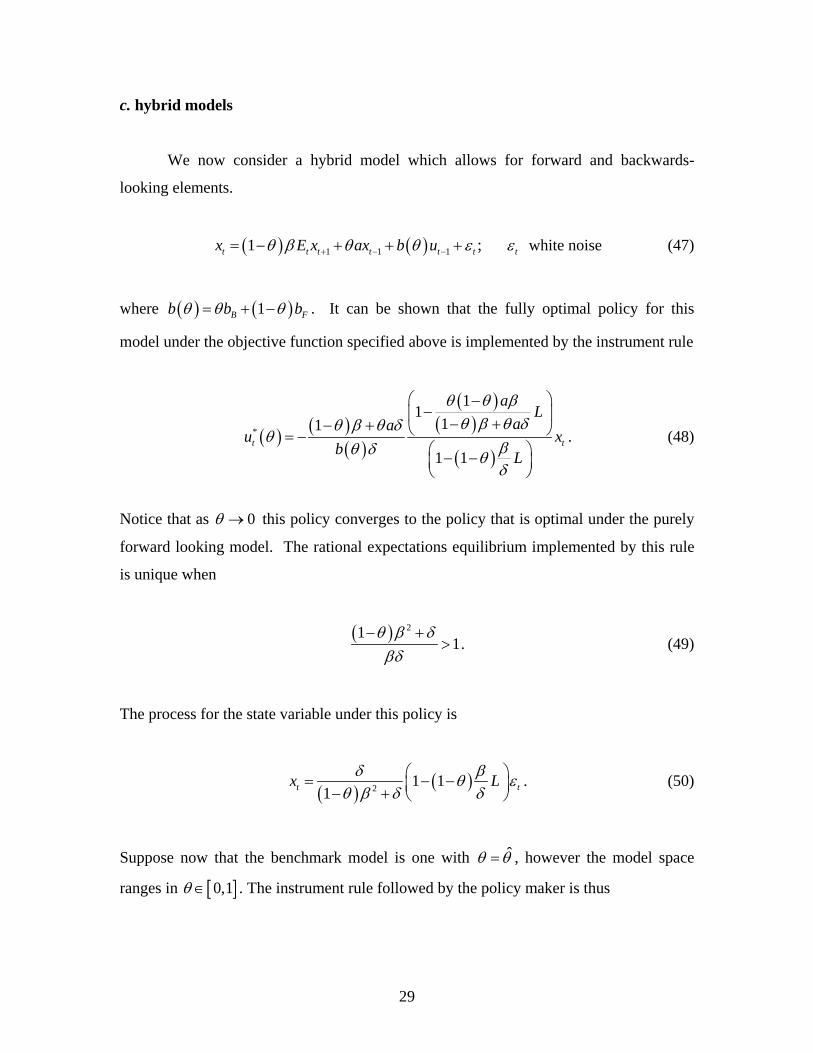
c. hybrid models

We now consider a hybrid model which allows for forward and backwards-

looking elements.

( ) ( )1 1 11t t t t t tx E x ax b u tθ β θ θ ε+ − −= − + + + ; ε

Fb

white noise (47)

where . It can be shown that the fully optimal policy for this

model under the objective function specified above is implemented by the instrument rule

( ) ( )1Bb bθ θ θ= + −

( ) ( )( )

( )( )

( )*

11

11

1 1t t

aL

aau x

b L

θ θ βθ β θ δθ β θ δ

θβθ δ θδ

⎛ ⎞−−⎜ ⎟− +− + ⎝= −⎛ ⎞− −⎜ ⎟⎝ ⎠

⎠ . (48)

Notice that as 0θ → this policy converges to the policy that is optimal under the purely

forward looking model. The rational expectations equilibrium implemented by this rule

is unique when

( ) 211

θ β δβδ

− +> . (49)

The process for the state variable under this policy is

( ) ( )2 1 11tx δ β

tLθ εθ β δ δ

⎛= − −⎜− + ⎝ ⎠⎞⎟ . (50)

Suppose now that the benchmark model is one with ˆθ θ= , however the model space

ranges in [ ]0,1θ ∈ . The instrument rule followed by the policy maker is thus

29

( ) ( )( )

( )( )( )( )

*ˆˆ 1

ˆˆ ˆ1

t

B Lu

b L

θα θθ

θ γ θ

−=

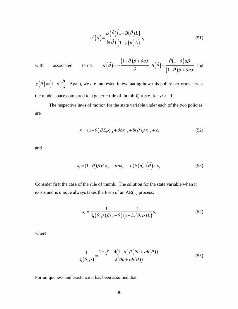
− tx (51)

with associated terms ( ) ( ) ( ) ( )( )

ˆ ˆ ˆ ˆ1 1ˆ ˆ, ,

ˆ ˆ1

a aB

a

θ β θ δ θ θ βα θ θ

δ θ β θ δ

− + −= − =

− +and

( ) ( )ˆ ˆ1 .βγ θ θδ

= − Again, we are interested in evaluating how this policy performs across

the model space compared to a generic rule of thumb t tu xρ= for 1ρ < − .

The respective laws of motion for the state variable under each of the two policies

are

( ) ( )1 1 11t t t t tx E x ax b x tθ β θ θ ρ ε+ − −= − + + + (52)

and

( ) ( ) ( )*1 1 1

ˆ1t t t t tx E x ax b u tθ β θ θ θ+ − −= − + + +ε . (53)

Consider first the case of the rule of thumb. The solution for the state variable when it

exists and is unique always takes the form of an AR(1) process:

( ) ( ) ( )( )1 2

1 1, 1 1 ,tx

L tελ θ ρ β θ λ θ ρ=

− − (54)

where

( )

( ) ( )( )( )( )

1 1 4 11, 2i

a b

a b

θ β θ ρ θ

λ θ ρ θ ρ θ

± − − +=

+. (55)

For uniqueness and existence it has been assumed that

30

( ) ( )1 2, 1, ,λ θ ρ λ θ ρ> 1< . (56)

This makes clear that a good rule of thumb is one where 1ρ > − because it ensures

uniqueness and existence of a bounded solution, i.e. it ensures (54) holds under many

specifications for θ ; as such this is a version of the Taylor principle.

For the optimal rule in our generic hybrid model, it can be shown that the law of

motion for the system is

( ) ( )( ) ( ) ( ) ( )( )1 1 2ˆ ˆ ˆ1 1 , , 1t t t t t

ˆtx L E x H x K x Lθ β γ θ θ θ θ θ γ θ+ − −= − − + + + − ε . (57)

Where ( ) ( ) ( )( )( )

ˆˆ ˆ,

ˆH a b

b

α θθ θ γ θ θ θ

θ≡ + + and ( ) ( ) ( )

( ) ( )( )

ˆ ˆˆ ˆ,

ˆB

K a bb

α θ θθ θ θ γ θ θ

θ= − − . The

primary issue for evaluating this rule under model uncertainty is the following. When the

policymaker is working with the correct model, the backwards-looking terms can be

shown to be zero, i.e. ( ) ( ), 0 and ,H Kθ θ θ θ= 0=

t

, but when the model is not correct

these terms are in general different than zero. This means that the dynamics of the system

become non trivial. It can be shown that the moving average representation of the state

variable, ( )tx G L ε= , is defined by

( )( )( ) ( )( )

( ) ( ) ( )( ) ( ) ( )( )0

2 3

ˆ1 1

ˆ ˆ1 1 1 , ,

L G LG L

L H L K L

γ θ θ β

θ β θ βγ θ θ θ θ θ

− − −=

− − + − + + ˆ. (58)

This representation is neither unique nor bounded unless restrictions are imposed in the

roots of the autoregressive polynomial. Writing the polynomial as

( ) ( )( ) ( )( ) ( )( )1 2 3ˆ ˆ1 1 , 1 , 1 ,L Lθ β λ θ θ λ θ θ λ θ θ− − − − ˆ L (59)

31

the condition for a unique and bounded solution is

( ) ( ) ( )1 2 3ˆ ˆ, 1, , 1, ,λ θ θ λ θ θ λ θ θ> < ˆ 1< . (60)

We assume that this condition holds so that the solution is again an ARMA(2,1)

( )( )

( )( )( )( ) ( )( )1 2 3

ˆ11ˆ ˆ ˆ, 1 1 , 1 ,

t t

Lx

L L

γ θε

λ θ θ θ β λ θ θ λ θ θ

−=

− − −. (61)

This again illustrates how optimal rules can be the source of fluctuations because of

model uncertainty.

To make the analysis concrete, we perform a numerical calculation for the

parameters 0.9, 0.99, 0.9aβ δ= = = As before, we consider {.1,1}B

F

bb

∈ . We construct

the optimal rule based on the benchmark model ( )OB .5θ = ; this produces optimal rules

( ) ( )( )

* 1 0.221.63

1 0.45t t

Lu x

Lθ

−= −

− for .1B

F

bb

= for ( ) ( )( )

* 1 0.220.90

1 0.45t t

Lu x

Lθ

−= −

− for 1B

F

bb

= . As

before, our rule of thumb is 11.25tu tx −= − . In all cases, a unique bounded rational

expectations equilibrium for the state variable exists. Figure 3 provides the overall and

frequency interval performances of the two rules as well as the associated values of the

Bode integral constraint. Tables 4 and 5 describe the minimum, maximum, and average

losses for the rules as well as minimax and minimax regret calculations.

Figure 3 describes the relative performances of the optimal rule for the benchmark

model versus the rule of thumb across the model space, for the case .1B

F

bb

= . As the

Figure indicates, for overall variance the rule of thumb outperforms the benchmark

optimal rule for smaller values of θ . This indicates an asymmetry in the effects of

overestimating versus underestimating the role of forward-looking elements.

32

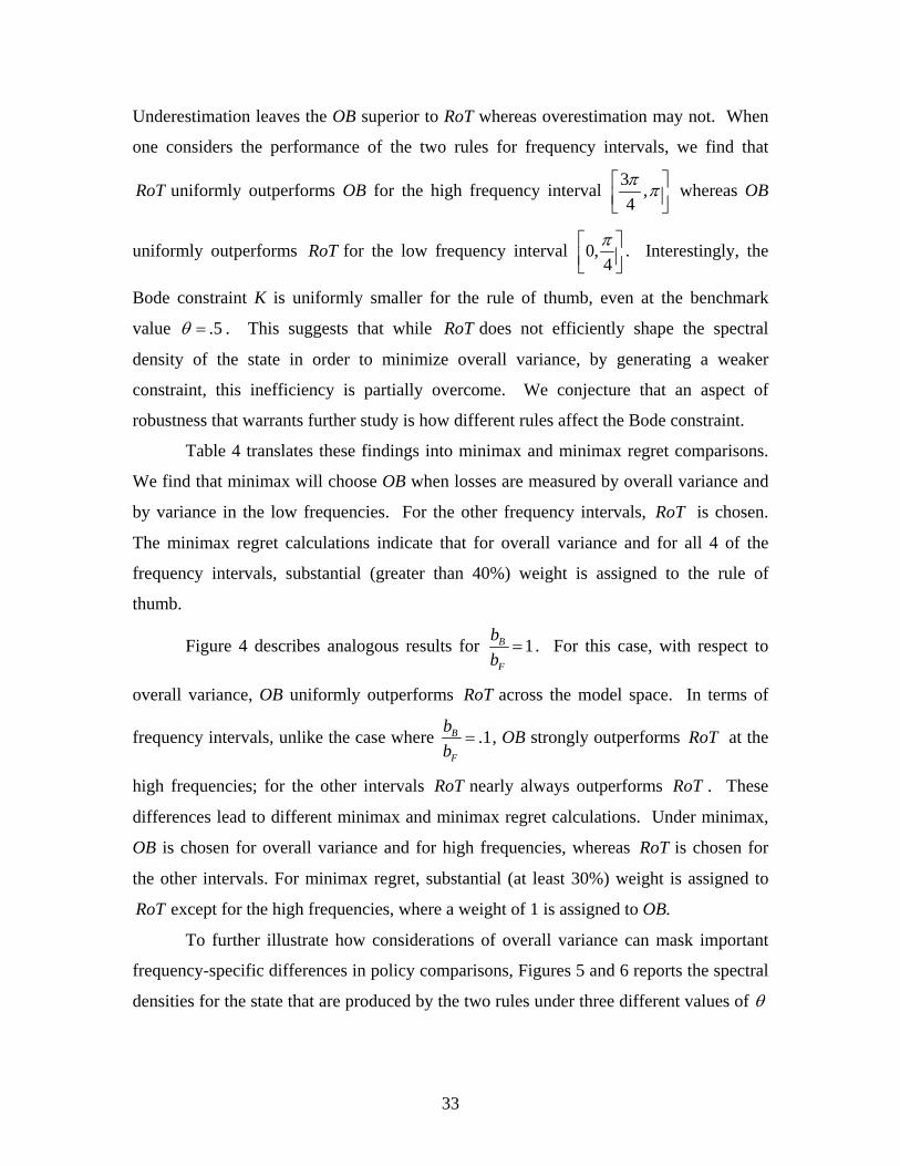
Underestimation leaves the OB superior to RoT whereas overestimation may not. When

one considers the performance of the two rules for frequency intervals, we find that

RoT uniformly outperforms OB for the high frequency interval 3 ,4π π⎡ ⎤

⎢ ⎥⎣ ⎦ whereas OB

uniformly outperforms RoT for the low frequency interval 0,4π⎡ ⎤

⎢ ⎥⎣ ⎦. Interestingly, the

Bode constraint K is uniformly smaller for the rule of thumb, even at the benchmark

value .5θ = . This suggests that while RoT does not efficiently shape the spectral

density of the state in order to minimize overall variance, by generating a weaker

constraint, this inefficiency is partially overcome. We conjecture that an aspect of

robustness that warrants further study is how different rules affect the Bode constraint.

Table 4 translates these findings into minimax and minimax regret comparisons.

We find that minimax will choose OB when losses are measured by overall variance and

by variance in the low frequencies. For the other frequency intervals, RoT is chosen.

The minimax regret calculations indicate that for overall variance and for all 4 of the

frequency intervals, substantial (greater than 40%) weight is assigned to the rule of

thumb.

Figure 4 describes analogous results for 1B

F

bb

= . For this case, with respect to

overall variance, OB uniformly outperforms RoT across the model space. In terms of

frequency intervals, unlike the case where .1B

F

bb

= , OB strongly outperforms RoT at the

high frequencies; for the other intervals RoT nearly always outperforms RoT . These

differences lead to different minimax and minimax regret calculations. Under minimax,

OB is chosen for overall variance and for high frequencies, whereas RoT is chosen for

the other intervals. For minimax regret, substantial (at least 30%) weight is assigned to

RoT except for the high frequencies, where a weight of 1 is assigned to OB.

To further illustrate how considerations of overall variance can mask important

frequency-specific differences in policy comparisons, Figures 5 and 6 reports the spectral

densities for the state that are produced by the two rules under three different values of θ

33

for the true model. Figure 5 assumes .1B

F

bb

= ; Figure 6 assumes 1B

F

bb

= . First consider

the case where the benchmark model is the true one, i.e. .5θ = , so that the model-

specific optimal rule is by construction variance minimizing. The figures indicate how

sensitive the comparison of rules is to frequency weighting as the fact that the optimal

rule produces lower overall variance than the rule of thumb does not mean that this

superiority is uniform across frequencies. For the case where the benchmark model is the

true one, i.e. .5θ = , the superior performance of the optimal rule when .1B

F

bb

= is due to

the variance reductions it produces in high frequencies whereas for 1B

F

bb

= the superior

performance is due to the variance reductions in the lower frequencies. In both cases,

there are intervals of frequencies where the rule of thumb outperforms the optimal rule.

This illustrates how model uncertainty and preference uncertainty with respect to

frequency weightings make it difficult to compare rules. The Figures also compare rule

performance for .25θ = and .75θ = . Overall, the relative performance of the optimal

rule and rule of thumb when compared across frequencies are similar to what was

observed for .5θ = ; this is so even though the spectral densities for .1B

F

bb

= are shaped

quite differently from the case for the benchmark model.

From the perspective of this exercise, we conclude that the case for the

benchmark optimal with respect over a rule of thumb is moderately strong in the presence

of model uncertainty concerning the role of forward versus backwards looking elements,

if one takes a strong stand that the loss function is the overall variance of the state.

However, the case is far weaker when allows for the possibility that the policymaker put

different weights on different frequency-specific fluctuations.

5. Taylor versus optimal rules in an IS/PC framework

34

In this section we apply our various ideas to the evaluation of the Taylor rule

versus an optimal rule for a two equation IS/PC system. TO BE COMPLETED

6. Summary and conclusions

Our basic conclusion is that the support for optimal rules versus Taylor’s original

rule is ambiguous when one considers the performance of the rules in the presence of

model uncertainty and with respect to frequency-specific effects. Further we observe that

the potential for optimal rules to go awry seems greater, especially for particular

frequency-specific intervals. This suggests to us that great caution should be taken in

seriously advocating inflation targeting, at least on the basis that they are optimal with

respect to a particular dynamic programming problem. While we are not so nihilistic as

to believe such knowledge is impossible, we believe that it is often the case that

contemporaneous scholarly discussions of macroeconomic policy pay too little attention

to Friedman’s 1948 arguments. Indeed, our analysis is more interventionist than his in

that our simple rules are versions of leaning against the wind policies, which Friedman

specifically questions because of the problem of long and variable lags in policy effects.

We do not think it unfair to say that modern time series analysis has led to a more

optimistic view of the information available to policymakers than assumed by

Friedman.16 Hence, we are comfortable with recommendations that are more

interventionist than his.17

A major weakness in our analysis is that we focus on comparisons of permanent

rule choices. In other words, we ask whether a policymaker should permanently choose

one rule or another. While this is the standard procedure in most of the monetary rules

literature, the analysis fails to address how a rule should be chosen when the policymaker

has the option of changing it in response to new information that affects the model space

under consideration. One solution is suggested by Svensson and Williams (2005) who

16In fact, Friedman (1972) acknowledges some progress of this type, although worry about politicization preserves his skepticism of countercyclical monetary policy. 17As such, we are sympathetic to the common sense spirit of Blinder (1998) though in our parlance a rule can react to the state of the economy.

35

treat different models as regimes across which the economy switches; in their analysis the

model uncertainty facing a policymaker is equivalent to uncertainty about the regime in

which the economy is currently in as the conditional probabilities of future regimes given

the current regime state. This is a promising research direction and admits progress using

Markov jump process methods, but it treats model uncertainty in a very different way

than we conceptualize it. In our approach, model uncertainty represents something that

may be resolved over time, not something that exists in a steady state. Hence the next

step in the approach we take seems likely to draw from ideas from the theory of bandit

problems rather than Markov jump processes. And of course both approaches to model

uncertainty cannot address the issue of policy evaluation when new elements emerge in

the model space over time. This problem begins to link monetary policy evaluation with

issues that lie at the frontiers of the work on decisionmaking under ambiguity, where

even the most advanced treatment typically assumes that while the probabilities are not

available for the object of interest, its support is known. So, we see this paper as only a

first step in a long research program.

36

Table 1

Panel A: Losses Over the Model Space ( )0.05, 0.95a a a∈ = = Total

Variance

Low

Freq.

[ ]40, π

Middle-

Low

[ ]4 2,π π

Middle-

High

[ ]32 4,π π

High

[ ]34 ,π π

Min Loss 1.00 0.12 0.17 0.17 0.12

Max Loss 1.25 0.66 0.30 0.30 0.66

2a a+

Average Loss 1.08 0.29 0.24 0.24 0.29

Min Loss 1.00 0.17 0.20 0.13 0.10

Max Loss 1.73 1.21 0.30 0.29 0.41

1 .3a =

Average Loss 1.15 0.46 0.27 0.21 0.20

Min Loss 1.00 0.09 0.12 0.22 0.19

Max Loss 2.29 0.33 0.28 0.30 1.80

1 .8a =

Average Loss 1.25 0.17 0.19 0.28 0.61

Panel B: Minimax (M) and Minimax Regret (MR)

12

a aWeight δ+⎛ ⎞ = −⎜ ⎟⎝ ⎠

Total

Variance

Low

Freq.

[ ]40, π

Middle-

Low

[ ]4 2,π π

Middle-

High

[ ]32 4,π π

High

[ ]34 ,π π

M MR M MR M MR M MR M MR

( )1 .3aδ = 0 .26 0 .31 0 .42 1 .58 1 .66

( )1 .8aδ = 0 .16 1 .73 1 .62 0 .37 0 .22

37

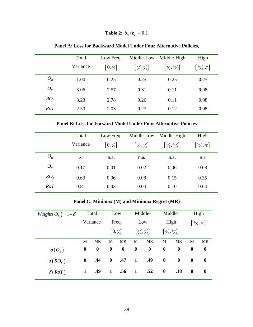
Table 2: / 0B Fb b .1=

Panel A: Loss for Backward Model Under Four Alternative Policies, Total

Variance

Low Freq.

[ ]40, π

Middle-Low

[ ]4 2,π π

Middle-High

[ ]32 4,π π

High

[ ]34 ,π π

BO 1.00 0.25 0.25 0.25 0.25

FO 3.06 2.57 0.31 0.11 0.08

FRO 3.23 2.78 0.26 0.11 0.08

RoT 2.50 2.03 0.27 0.12 0.08

Panel B: Loss for Forward Model Under Four Alternative Policies

Total

Variance

Low Freq.

[ ]40, π

Middle-Low

[ ]4 2,π π

Middle-High

[ ]32 4,π π

High

[ ]34 ,π π

BO ∞ n.a. n.a. n.a. n.a

FO 0.17 0.01 0.02 0.06 0.08

FRO 0.63 0.06 0.08 0.15 0.35

RoT 0.81 0.03 0.04 0.10 0.64

Panel C: Minimax (M) and Minimax Regret (MR)

( ) 1FWeight O δ= − Total

Variance

Low

Freq.

[ ]40, π

Middle-

Low

[ ]4 2,π π

Middle-

High

[ ]32 4,π π

High

[ ]34 ,π π


( )BOδ 0 0 0 0 0 0 0 0 0 0

( )FROδ 0 .44 0 .47 1 .49 0 0 0 0

( )RoTδ 1 .49 1 .56 1 .52 0 .18 0 0

38

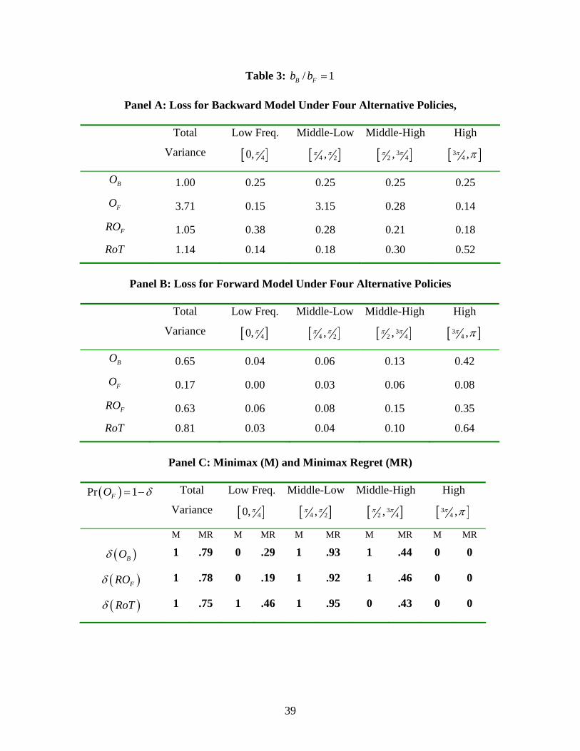
Table 3: / 1B Fb b =

Panel A: Loss for Backward Model Under Four Alternative Policies, Total

Variance

Low Freq.

[ ]40, π

Middle-Low

[ ]4 2,π π

Middle-High

[ ]32 4,π π

High

[ ]34 ,π π

BO 1.00 0.25 0.25 0.25 0.25

FO 3.71 0.15 3.15 0.28 0.14

FRO 1.05 0.38 0.28 0.21 0.18

RoT 1.14 0.14 0.18 0.30 0.52

Panel B: Loss for Forward Model Under Four Alternative Policies

Total

Variance

Low Freq.

[ ]40, π

Middle-Low

[ ]4 2,π π

Middle-High

[ ]32 4,π π

High

[ ]34 ,π π

BO 0.65 0.04 0.06 0.13 0.42

FO 0.17 0.00 0.03 0.06 0.08

FRO 0.63 0.06 0.08 0.15 0.35

RoT 0.81 0.03 0.04 0.10 0.64

Panel C: Minimax (M) and Minimax Regret (MR)

( )Pr 1FO δ= − Total

Variance

Low Freq.

[ ]40, π

Middle-Low

[ ]4 2,π π

Middle-High

[ ]32 4,π π

High

[ ]34 ,π π


( )BOδ 1 .79 0 .29 1 .93 1 .44 0 0

( )FROδ 1 .78 0 .19 1 .92 1 .46 0 0

( )RoTδ 1 .75 1 .46 1 .95 0 .43 0 0

39

Table 4

Panel A: Losses Over the Model Space ( )0,1θ ∈ , / .B Fb b = 1

Total

Variance

Low

Freq.

[ ]40, π

Middle-

Low

[ ]4 2,π π

Middle-

High

[ ]32 4,π π

High

[ ]34 ,π π

Min Loss 0.78 0.01 0.03 0.10 0.09

Max Loss 1.88 1.35 0.42 0.29 0.79

OB

( ).5θ = Average Loss 0.99 0.22 0.20 0.20 0.37

Min Loss 0.76 0.03 0.04 0.10 0.09

Max Loss 2.40 1.91 0.35 0.25 0.63

RoT

( 1.25ρ = − ) Average Loss 1.07 0.37 0.19 0.19 0.33


( )Pr 1OB δ= − Total

Variance

Low Freq.

[ ]40, π

Middle-Low

[ ]4 2,π π

Middle-High

[ ]32 4,π π

High

[ ]34 ,π π


( )RoTδ 0 .41 0 .41 1 .54 1 .55 1 .57

40

Table 5

Panel A: Losses Over the Model Space ( )0,1θ ∈ , / 1B Fb b =

Total

Variance

Low

Freq.

[ ]40, π

Middle-

Low

[ ]4 2,π π

Middle-

High

[ ]32 4,π π

High

[ ]34 ,π π

Min Loss 0.61 0.03 0.06 0.15 0.21

Max Loss 1.05 0.18 0.37 0.32 0.37

OB

( ).5θ = Average Loss 0.84 0.08 0.18 0.25 0.33

Min Loss 0.81 0.03 0.04 0.10 0.52

Max Loss 1.14 0.14 0.18 0.30 0.68

RoT

( 1.25ρ = − ) Average Loss 0.99 0.07 0.09 0.19 0.64


( )Pr 1OB δ= − Total

Variance

Low Freq.

[ ]40, π

Middle-Low

[ ]4 2,π π

Middle-High

[ ]32 4,π π

High

[ ]34 ,π π


( )RoTδ 0 .31 1 .58 1 .73 1 .59 0 0

41

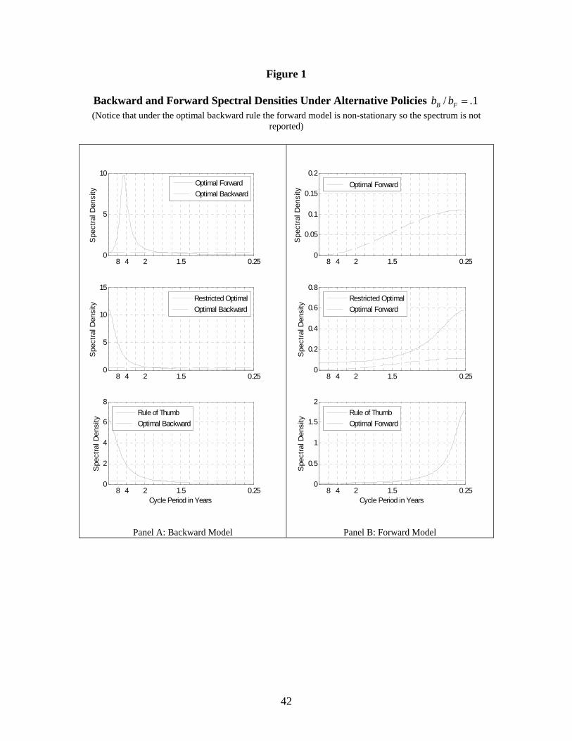
Figure 1

Backward and Forward Spectral Densities Under Alternative Policies / .B Fb b 1= (Notice that under the optimal backward rule the forward model is non-stationary so the spectrum is not

reported)

8 4 2 1.5 0.250

5

10

Spe

ctra

l Den

sity

Optimal ForwardOptimal Backward

8 4 2 1.5 0.250

5

10

15

Spe

ctra

l Den

sity

Restricted OptimalOptimal Backward

8 4 2 1.5 0.250

2

4

6

8

Cycle Period in Years

Spe

ctra

l Den

sity

Rule of ThumbOptimal Backward

Panel A: Backward Model

8 4 2 1.5 0.250

0.05

0.1

0.15

0.2

Spe

ctra

l Den

sity

8 4 2 1.5 0.250

0.2

0.4

0.6

0.8

Spe

ctra

l Den

sity

8 4 2 1.5 0.250

0.5

1

1.5

2


Spe

ctra

l Den

sity

Optimal Forward

Restricted OptimalOptimal Forward

Rule of ThumbOptimal Forward

Panel B: Forward Model

42

Figure 2

Backward and Forward Spectral Densities Under Alternative Policies / 1B Fb b =

8 4 2 1.5 0.250

5

10

15

Spe

ctra

l Den

sity

8 4 2 1.5 0.250.2

0.3

0.4

0.5

0.6

0.7

Spe

ctra

l Den

sity

8 4 2 1.5 0.250

0.2

0.4

0.6

0.8


Spe

ctra

l Den

sity

Optimal ForwardOptimal Backward

Restricted OptimalOptimal Backward

Rule of ThumbOptimal Backward

Panel A: Backward Model

8 4 2 1.5 0.250

0.5

1

Spe

ctra

l Den

sity

8 4 2 1.5 0.250

0.2

0.4

0.6

0.8

Spe

ctra

l Den

sity

8 4 2 1.5 0.250

0.5

1

1.5

2


Spe

ctra

l Den

sity

Optimal BackwardOptimal Forward

Restricted OptimalOptimal Forward

Rule of ThumbOptimal Forward

Panel B: Forward Model

43

Figure 3. Frequency Specific Losses and Bode Constraint

/ .B Fb b 1=

0 0.5 10.5

1

1.5

2

2.5

Model Space

Tota

l Var

ianc

e

Optimal RuleRule of Thumb

0 0.5 1-0.8

-0.6

-0.4

-0.2

0

0.2

Model Space

Bod

e C

onst

rain

t K

0 0.5 10

0.5

1

1.5

2

Model Space

Var

ianc

e Lo

w F

req

0 0.5 10

0.1

0.2

0.3

0.4

0.5

Model Space

Var

ianc

e M

iddl

e-Lo

w F

req

0 0.5 10.05

0.1

0.15

0.2

0.25

0.3

Model Space

Var

ianc

e M

iddl

e-H

igh

Freq

0 0.5 10

0.2

0.4

0.6

0.8

Model Space

Var

ianc

e H

igh

Freq

44

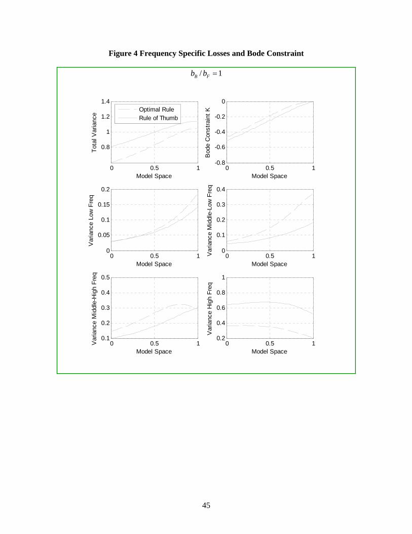
Figure 4 Frequency Specific Losses and Bode Constraint

/ 1B Fb b =

0 0.5 1

0.8

1

1.2

1.4

Model Space

Tota

l Var

ianc

e


0 0.5 1-0.8

-0.6

-0.4

-0.2

0

Model Space

Bod

e C

onst

rain

t K

0 0.5 10

0.05

0.1

0.15

0.2

Model Space

Var

ianc

e Lo

w F

req

0 0.5 10

0.1

0.2

0.3

0.4

Model Space

Var

ianc

e M

iddl

e-Lo

w F

req

0 0.5 10.1

0.2

0.3

0.4

0.5

Model Space

Var

ianc

e M

iddl

e-H

igh

Freq

0 0.5 10.2

0.4

0.6

0.8

1

Model Space

Var

ianc

e H

igh

Freq

45

Figure 5: Variance Decomposition Under Optimal Rule for Benchmark Model ( / 0B Fb b .1= )

8 4 2 1.5 0.250.05

0.1

0.15

0.2

0.25

0.3

0.35

0.4

0.45

0.5


Spe

ctra

l Den

sity


Panel A: Benchmark Model ( .5θ = )

8 4 2 1.5 0.250

0.1

0.2

0.3

0.4

0.5

0.6

0.7

0.8

0.9

1


Spe

ctra

l Den

sity


Panel B.1: .25θ =

8 4 2 1.5 0.250.2

0.3

0.4

0.5

0.6

0.7

0.8

0.9


Spe

ctra

l Den

sity


Panel B.2: .75θ =

46

Figure 6: Variance Decomposition Under Optimal Rule for Benchmark Model ( / 1.B Fb b 0= )

8 4 2 1.5 0.250

0.2

0.4

0.6

0.8

1

1.2

1.4


Spe

ctra

l Den

sity


Panel A: Benchmark Model ( .5θ = )

8 4 2 1.5 0.250

0.2

0.4

0.6

0.8

1

1.2

1.4

1.6

1.8


Spe

ctra

l Den

sity


Panel B.1: .25θ =

8 4 2 1.5 0.250.1

0.2

0.3

0.4

0.5

0.6

0.7

0.8

0.9

1

1.1


Spe

ctra

l Den

sity


Panel B.2: .75θ =

47

Technical Appendix

Section 4.a: Derivation of minimax regret policies for optimal and rule of thumb policies under parameter uncertainty

In calculating the minimax regret solution when the candidate policies are and 1a

2 2a aa +

= , the maximum regret ( )1MR a will depend on the value of with respect to

the alternative policy. One therefore needs to consider two cases

1a

( ) ( )( )

21

1 1 21

2 1a aa aa MR a

a a−+

⇒ =− −

Case L: < (62)

and

( ) ( )( )

21

1 1 21

Case H: . 2 1

a aa a a MR aa a−+

< ⇒ =− −

(63)

In either case,

( ) ( )( )

2

2 21 1

412

a aMR a

a aa a

⎛ ⎞⎜ ⎟ −⎜ ⎟= − =⎜ ⎟ − −−⎛ ⎞−⎜ ⎟⎜ ⎟

⎝ ⎠⎝ ⎠

2 . (64)

It follows that the minimax regret rules are different across the two cases, which are

given in eq. (27).

Section 4.a: Frequency-specific losses

48

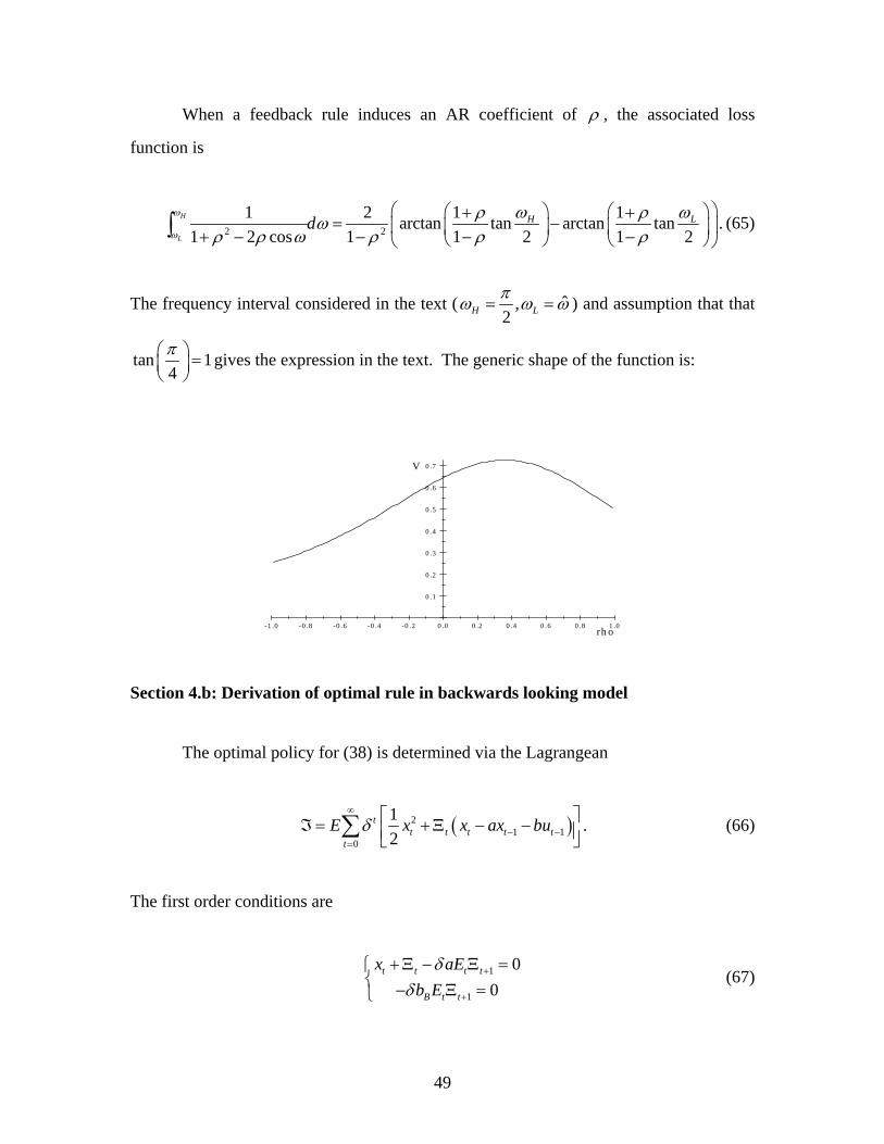
When a feedback rule induces an AR coefficient of ρ , the associated loss

function is

2 2

1 2 1 1arctan tan arctan tan1 2 cos 1 1 2 1 2

H

L

H Ldω

ω

ω ωρ ρωρ ρ ω ρ ρ ρ

⎛ ⎞⎛ ⎞ ⎛+ += −⎜ ⎟⎜ ⎟ ⎜+ − − − −⎝ ⎠ ⎝⎝ ⎠

∫⎞⎟⎠

. (65)

The frequency interval considered in the text ( ˆ,2H Lπω ω ω= = ) and assumption that that

tan 14π⎛ ⎞ =⎜ ⎟⎝ ⎠

gives the expression in the text. The generic shape of the function is:

-1 .0 -0 .8 -0 .6 -0 .4 -0 .2 0 .0 0 .2 0 .4 0 .6 0 .8 1 .0

0 .1

0 .2

0 .3

0 .4

0 .5

0 .6

0 .7

rh o

V

Section 4.b: Derivation of optimal rule in backwards looking model

The optimal policy for (38) is determined via the Lagrangean

(21 1

0

12

tt t t t t

tE x x ax buδ

∞

− −=

)⎡ ⎤ℑ = +Ξ − −⎢ ⎥⎣ ⎦∑ . (66)

The first order conditions are

1

1

00

t t t t

B t t

x aEb Eδ

δ+

+

+ Ξ − Ξ =⎧⎨ − Ξ =⎩

(67)

49

It follows that

tx t= −Ξ (68)

and so

1 1 0t t t tE x E+ += − Ξ = . (69)

Applying the expectations operator it is evident that

1

0t t t B t t t

t B t

E x ax b u Eax b u

1ε+ += + += +

(70)

which leads to the optimal rule backward looking rule reported in the text.

Section 4.b: Derivation of Optimal Forward Looking Rule

The Lagrangean for (38) is

(21 1

0

12

tt t t t t

tE x x x buδ β

∞

+ −=

)⎡ ⎤ℑ = +Ξ − −⎢ ⎥⎣ ⎦∑ (71)

which produces first order conditions

1

1

0

0

t t t

F t t

x

b E

βδ

δ

−

+

⎧ +Ξ − Ξ =⎪⎨⎪ − Ξ =⎩

(72)

so that

50

1t tx Lβδ

⎛= −Ξ −⎜⎝ ⎠

⎞⎟ . (73)

Leading the forward model one period and substituting

1 1 11t t t t t t t tE x E L Eβ β βδ δ δ+ + +

⎛ ⎞= − Ξ − = − Ξ + Ξ = Ξ⎜ ⎟⎝ ⎠

. (74)

Substituting into the Lagrangean constraint

2

11t t FL b uβ βt tεδ δ −

⎛ ⎞−Ξ − = Ξ + +⎜ ⎟⎝ ⎠

. (75)

Leading this forward one period and taking expectations

t F t t Fb u b utβ δδ βΞ = ⇒ Ξ = (76)

so that

1t F tx b Lδ ββ δ

⎛= − −⎜⎝ ⎠

u⎞⎟ (77)

which leads to the expression in the text.

Section 4.c: Fully optimal rule for a hybrid model

The (unconditional) Lagrangean for this problem is

( ) ( )( )21 1

0

1 12

tt t t t t t

t

E x x x ax b uδ θ β θ∞

+ − −=

⎡ ⎤ℑ = +Ξ − − − −⎢ ⎥⎣ ⎦∑ 1θ (78)

51

where

( ) ( )1Bb bθ θ θ= + − Fb . (79)

The set of first order conditions are

( )

( )1

1

1 0

0

t t t t t

t t

x a

b E

βθ θ δδ

δ θ

− +

+

⎧ + Ξ − − Ξ − Ξ =⎪⎨⎪ − Ξ =⎩

1E (80)

It immediately follows that

( )1 1t tx Lβθδ

⎛= −Ξ − −⎜⎝ ⎠

⎞⎟ (81)

and so

( ) ( )1 1 1 1 1t t t t tE x E Lβ βθ θδ δ+ +

⎡ ⎤⎛ ⎞= − Ξ − − = − Ξ⎜ ⎟⎢ ⎥⎝ ⎠⎣ ⎦. (82)

Substituting the expressions for tx and into the hybrid constraint one finds the

relationship that the multiplier and the instrument must obey on an optimal path,

( ) ( ) ( ) ( )2

1 11 1 1 1 1t t tL a L bβ β βt tuθ θ θ θ θ

δ δ δ− −⎛ ⎞ ⎛ ⎞−Ξ − − = − − Ξ − Ξ − − + +⎜ ⎟ ⎜ ⎟⎝ ⎠ ⎝ ⎠

ε . (83)

Leading this equation forward one period and applying the expectation operator to it

produces

52

( ) ( ) ( )1 1 1t ta Lβ βtb uθ θ θ

δ δ⎛ ⎞− Ξ = − Ξ − − +⎜ ⎟⎝ ⎠

θ (84)

rearranging the instrument and the multiplier are related by:

( ) ( ) ( )

( )( ) ( )

( )( )

( )( )

1 1 1

11 1

1 11 .

1

t

t

t

t

uaa L

b

a a Lb

a aL

b a

β βθ θ θ θθ δ δ

θ β δθ βθ θθ δ δ

θ β δθ θ θ βθ δ θ β δθ

=

⎛ ⎞− + − − Ξ =⎜ ⎟⎝ ⎠

− +⎛ ⎞− −⎜ ⎟

⎝ ⎠⎛ ⎞− + −

Ξ =

− Ξ⎜ ⎟⎜ ⎟− +⎝ ⎠

(85)

Notice that as 0θ → this condition delivers the relationship between the multiplier and

the instrument for the pure forward looking case.

We next consider the optimal relationship between the instrument and the state

which is bridged by the process for the multiplier. Let ( ) ( )1 aθ β δθα θ

δ− +

≡ − ,

( ) ( )1 βγ θ θδ

≡ − , ( ) ( )( )

11

aB

aθ θ β

θθ β δθ−

≡− +

and assume that ( ) 1ξ θ < so that we can

write the multiplier in terms of the instrument and substituting

( ) ( )( )( ) ( )( )

11t

b Ltx u

B Lθ γ θ

α θ θ−

=−

(86)

from which, under the assumption ( )1 βθδ

1− < , one can derive the optimal instrument

rule

53

( ) ( )( )

( )( )( )( )

( )( )

( )( )

( )

* 11

11

11.

1 1

t t

t

B Lu x

b L

aL

aax

b L

θα θθ

θ γ θ

θ θ βθ β δθθ β δθ

βθ δ θδ

−= =

−

⎛ −−⎜

− +− + ⎝ ⎠−⎛ ⎞− −⎜ ⎟⎝ ⎠

⎞⎟ (87)

An instrument rule combined with the law of motion for the state allows to write an

expectational difference equation only in terms of the state. In what follows we solve for

the path of the state variable tx by applying the instrument rule for a benchmark model

θ̂ , ( ) ( )( )

( )( )( )( )

*ˆˆ 1

ˆˆ ˆ1

t

B Lu

b L

θα θθ

θ γ θ

−=

−tx , to a law of motion of a generic model θ which, namely

we want to solve for

( ) ( )( )( )

( )( )( )( )1 1 1

ˆˆ 11

ˆ ˆ1t t t t t

B Lx E x ax b x

b L

θα θtθ β θ θ

θ γ θ+ − −

−= − + + +

−ε . (88)

Multiply both sides of (88) by ( )( ˆ1 Lγ θ− ) so that the equation becomes

( )( ) ( )( )( ) ( )( )( )

( )( ) ( )( ) ( )( )

1 1

1

ˆ ˆ ˆ1 1 1 1

ˆˆ ˆ1 1

ˆ

t t t

t t

L x L E x L ax

b B L x Lb

γ θ γ θ θ β γ θ θ

α θθ θ γ θ ε

θ

t+ −

−

− = − − + −

+ − + − (89)

or

54

( ) ( )( ) ( ) ( )( )( )

( ) ( )( )( ) ( ) ( )( )

1 1

2

ˆˆ ˆ1 1

ˆ

ˆˆ ˆ ˆ1 .

ˆ

t t t t t

t t

1tx E x E x a b xb

a b B x Lb

α θθ β γ θ θ β γ θ θ θ

θ

α θγ θ θ θ θ γ θ ε

θ

+ −

−

⎛ ⎞⎜ ⎟= − − − + + +⎜ ⎟⎝ ⎠

⎛ ⎞⎜ ⎟− + + −⎜ ⎟⎝ ⎠

−

(90)

Let ( ) ( ) ( )( )( )

ˆˆ ˆ,

ˆH a b

b


θ

⎛ ⎞⎜ ⎟= + +⎜ ⎟⎝ ⎠

and ( ) ( ) ( )( )( ) ( )

ˆˆ ˆ,

ˆK a b

b

α θˆBθ θ γ θ θ θ θ

θ= − − .

It can be shown that when the optimal rule is applied to the appropriate model these two

objects take equal zero, i.e.

( ) ( ) ( ) ( )

( )

( ) ( )

,

11 0

H a bb

aa


θ

θ β δθβθ θδ δ

= + + =

− +− + − =

(91)

and

( ) ( ) ( ) ( )

( ) ( )

( ) ( ) ( )( )

,

1 11 0

1

K a b Bb

a aa

a

α θθ θ γ θ θ θ θ

θ

θ β δθ θ θ ββθ θδ δ θ β δθ

= − − =

− + −− − + =

− +. (92)

This shows that when the optimal policy is tailored to the wrong model higher order

dynamics are activated in the law of motion for the state. We solve the expectational

difference equation by guessing a square summable moving average form

( )ˆ,t tx G Lθ θ

ε= . (93)

55

Dropping the subscripts for notational convenience we have

( )( ) ( )( ) ( )( ) ( )(

( ) ( ) ( ) ( ) ( )( )1

0 0

2

ˆ1 1

ˆ ˆ, , 1

t

t t

t t

G L

G L G L G L G

H G L L K G L L L

ε

)ˆ .t

θ β ε γ θ θ β ε

θ θ ε θ θ ε γ θ

−

=

− − − − −

+ + + − ε

(94)

Multiplying both sides by , rearranging and making use of the Riesz-Fischer theorem

one can write

L

( )( )( ) ( )( )

( ) ( ) ( )( ) ( ) ( )( )0

2 3

ˆ1 1

ˆ ˆ1 1 1 , ,

L G LG L

L H L K L

γ θ θ β

θ β θ βγ θ θ θ θ θ

− − −=

− − + − + + ˆ. (95)

To ensure a unique solution exactly one root of the denominator must be inside the unit

circle (i.e. the dominant eigenvalue bigger than one) so that can be chosen in order to

exactly cancel this unstable root. The denominator can be always represented as:

0G

( ) ( )( ) ( )( ) ( )( )1 2 3ˆ ˆ1 1 , 1 , 1 ,L Lθ β λ θ θ λ θ θ λ θ θ− − − − ˆ L . (96)

In what follows we assume that for any combination we consider we have

( ) ( ) ( )1 2 3ˆ ˆ, 1, , , ,λ θ θ λ θ θ λ θ θ> ˆ 1< . (97)

If this is not satisfied there exists a set of solutions that satisfy the first order conditions.

The unique solution is identified by the condition

56

( ) ( ) ( )( )0 0

1 1

11 0ˆ ˆ, ,

G Gθ β 11λ θ θ λ θ θ θ β

⎛ ⎞⎜ ⎟− − = ⇒ =⎜ ⎟ −⎝ ⎠

. (98)

Finally, substituting in the generic solution and canceling the roots the solution becomes

( )( )( )

( )( ) ( )( ) ( )( )ˆ,1 2 3

ˆ1

ˆ ˆ, 1 1 , 1 ,

LG L

L Lθ θ

γ θ

λ θ θ θ β λ θ θ λ θ θ

−=

− − − ˆ. (99)

When the optimal rule is applied to the appropriate model the higher order dynamics

disappear and the solution becomes a simple MA(1)

( )( )( )

( )( )ˆ ˆ,1

ˆ1

ˆ ˆ ˆ, 1

LG L

θ θ

γ θ

λ θ θ θ β

−=

−. (100)

The normalized spectral densities reported in the main text are then computed by

evaluating the moving average on the unit circle, i.e. iL e ω−= ,

( ) ( ) (212

i ix )f G e G eω ω

εω σπ

−= . (101)

57

Bibliography

Blinder, A. 1998. Central Banking in Theory and Practice. Cambridge: MIT Press. Blume, L., D. Easley, and J. Halperin. 2006. Redoing the Foundations of Decision Theory. Mimeo, Cornell University. Brock. W. 2006. Profiling Problems With Partially Identified Structure. Economic Journal, forthcoming. Brock, W. and S. Durlauf. 2004. Elements of a Theory of Design Limits to Optimal Policy. The Manchester School, 72, Supplement 2, 1-18, 2004. Brock, W. and S. Durlauf, (2005), “Local Robustness Analysis: Theory and Application,” Journal of Economic Dynamics and Control 29, 11, 2067-2092. Brock, W., S. Durlauf, and G. Rondina. 2006. Design Limits and Dynamic Policy Analysis. Mimeo, University of Wisconsin. Brock, W., S. Durlauf and K. West. 2003. Policy Analysis in Uncertain Economic Environments (with discussion). Brookings Papers on Economic Activity 1, 235-322. Brock, W., S. Durlauf, K. West. 2006. Model Uncertainty and Policy Evaluation: Some Theory and Empirics. Journal of Econometrics, forthcoming. Camerer, C. and G. Loewenstein. 2003. Behavioral Economics: Past, Present, Future. “is in Advances in Behavioral Economics, C. Camerer, G. Loewenstein, and M. Rabin, eds. Princeton: Princeton University Press. Chamberlain, G. 2001. Econometrics and Decision Theory. Journal of Econometrics 95: 255-83. Chernoff, H. 1954. Rational Selection of Decision Functions. Econometrica 22: 422-443 Clarida, R., J. Gali and M. Gertler, 1999. The Science of Monetary Policy: A New Keynesian Perspective. Journal of Economic Literature XXXVII(December), 1661-1701 Epstein, L. and T. Wang. 1994. Intertemporal Asset Pricing Behavior Under Knightian Uncertainty. Econometrica, 62, 283-322. Freedman, D. 1991. A Rejoinder to Berk, Blalock, and Mason. Sociological Methodology 21, 353-358, 1991. Friedman, M. 1948. A Monetary and Fiscal Framework for Economic Stability. American Economic Review 38, 3, 245-264.

58

Friedman, M. 1972. Monetary Policy. Proceedings of the American Philosophical Society 116(3), 183-196. Giannoni, M. 2002. “Does Model Uncertainty Justify Caution? Robust Optimal Monetary Policy in a Forward-Looking Model.” Macroeconomic Dynamics 6: 111-144. Gilboa, I. and D. Schmeidler. 1989. Maximin Expected Utility with Non-Unique Priors. Journal of Mathematical Economics 18: 141-53. Hansen, L., T. Sargent. 2003. Robust Control of Forward-Looking Models. Journal of Monetary Economics, 50, 581-604. Hansen, L., T. Sargent. 2006. Robustness. manuscript, Hoover Institution, Stanford University and forthcoming, Princeton University Press. Hurwicz, L. 1951. Some Specification Problems and Applications to Econometric Models. Econometrica, 19, 343-4. Key, J., L. Perrichi, and A. Smith. 1998. Choosing Among Models when None of Them are True. In Proceedings of the Workshop on Model Selection, Special Issue of Rassegna di Metodi Statistici ed Applicazioni, W. Racugno, ed., Bologna: Pitagora Editrice. Leamer, E. 1978. Specification Searches. New York: John Wiley and Sons. Levin, A., J. Williams. 2003. Robust Monetary Policy with Competing Reference Models. Journal of Monetary Economics, 50, 5, 945-975. Manski, C. 2005. Statistical Treatment Rules for Heterogeneous Populations. Econometrica, 72, 1221-1246. Manski, C. 2006. Minimax-Regret Threatment Choice with Missing Outcome Data. Journal of Econometrics, forthcoming. McCallum, B. 1988. Robustness Properties of a Rule for Monetary Policy. Carnegie-Rochester Conference Series on Public Policy, 29, 173-204. McCallum, B. 1999. Issues in the Design of Monetary Policy Rules. Handbook of Macroeconomics, J. Taylor and B. McCallum, eds. Amsterdam: North-Holland, 1483-1530. McCallum, B. and E. Nelson. 2005. Targeting versus Instrument Rules for Monetary Policy. Federal Reserve Bank of St. Louis Review, September/October, 597-611. Onatski, A. and J. Stock. 2002. “Robust Monetary Policy Under Model Uncertainty in a Small Model of the U.S. Economy.” Macroeconomic Dynamics 6: 85-110.

59

Onatski, A. and N. Williams. 2003. Modeling Model Uncertainty. Journal of the European Economic Association, 1, 1078-1122. Otrok. C. 2001. Spectral Welfare Cost Functions. International Economic Review, 42, 345-367. Raftery, A., D. Madigan, and J. Hoeting. 1997. Bayesian Model Averaging for Linear Regression Models. Journal of the American Statistical Association, 92, 437, 179-91. Rudebusch, G. 2002. Assessing Nominal Income Rules for Monetary Policy with Model and Data Uncertainty. Economic Journal 112(April), 402-432. Rudebusch, G. and L. Svensson. 1999. Policy Rules for Inflation Targeting. In Monetary Policy Rules, J. Taylor, ed. Chicago: University of Chicago Press. Rudd, J. and K. Whelan. 2005. “New Tests of the new-Keyneisan Phillips Curve,” Journal of Monetary Economics 52, 1167-1181. Savage, L. J. 1951. The Theory of Statistical Decision. Journal of the American Statistical Association, 46, 55-67. Stoye, J. 2006. Statistical Decisions under Ambiguity. Mimeo, New York University. Targeting Rules. Journal of Economic Literature, 42, 2, 426-477. Svensson, L. 2002. Robust Control Made Simple. Mimeo, Princeton University. Svensson. L. 2003. What is Wrong with Taylor Rules? Using Judgment in Monetary Policy through Targeting Rules. Journal of Economic Literature, 42, 2, 426-477. Svensson, L. and N. Williams. 2005. Monetary Policy with Model Uncertainty: Distribution Foreacast Targeting. Mimeo, Princeton University. Taylor, J. 1993. Discretion Versus Policy Rules in Practice. Carnegie-Rochester Conference Series on Public Policy, 39, 195-214. Tetlow, R. and P. von zur Muehlen. 2001. Robust Monetary Policy with Misspecified Models: Does Model Uncertainty Always Call for Attenuated Policy? Journal of Economic Dynamics and Control 25, 6-7, 911-949. Tobin, J. 1983. Monetary Policy: Rules, Targets, and Shocks. Journal of Money, Credit, and Banking 15(4), 506-518. Wald, A., 1950. Statistical Decision Functions. John Wiley, New York.

60

Is the Original Taylor Rule Enough? Simple versus Optimal ... · Is the Original Taylor Rule...

Documents

Transcript of Is the Original Taylor Rule Enough? Simple versus Optimal ... · Is the Original Taylor Rule...