IS THE LEADERSHIP OF THE BRENT-WTI OIL FUTURES MARKET ...

IS THE LEADERSHIP OF THE BRENT-WTI OIL

FUTURES MARKET THREATENED?

Marta Roig Atienza

Trabajo de investigación 019/019

Master en Banca y Finanzas Cuantitativas

Director/a: Dr. Fernando Palao Sánchez

Dr. Ángel Pardo Tornero

Universidad Complutense de Madrid

Universidad del País Vasco

Universidad de Valencia

Universidad de Castilla-La Mancha

www.finanzascuantitativas.com

Is the leadership of the Brent-WTI oil futures

market threatened?

Marta Roig Atienza

MSc Thesis for the degree

MSc in Banking and Quantitative Finance

July 2019

Supervisors: Dr Fernando Palao Sánchez

Dr Ángel Pardo Tornero

Universidad Complutense de Madrid

Universidad del País Vasco

Universidad de Valencia

Universidad de Castilla-La Mancha

www.finanzascuantitativas.com

1

Agradecimientos

En primer lugar, quiero agradecer a mis tutores, Fernando Palao y Ángel Pardo,

su apoyo y ayuda desinteresada durante estos meses. He sido muy afortunada

de tenerles como tutores. La ilusión con la que ambos viven las finanzas y la

enseñanza se ha traducido en ilusión y ganas por trabajar en este proyecto

común. Además de esto, no encontraría una mejor forma de cerrar esta etapa,

ya que en mis estudios de grado Ángel fue quién me despertó mi interés por el

mundo de las finanzas cuantitativas.

Gracias a Jesús Ruíz por sus valiosos comentarios en el ámbito de la

econometría.

Gracias también a mi madre Bienve, a mi hermano Sergio y a mi tía Carmen.

Gracias por soportarme, siempre apoyarme en conseguir mis sueños y creer

muchas veces más en mí de lo que yo misma lo hago.

Por último, gracias a Ale por acompañarme a donde la magia ocurre. Ojalá que

por mucho que sople el viento, siempre vayamos hacía tramuntana.

2

Abstract

The relationship between crude oil prices is a topic that has often been addressed

in the energy economics literature. Especially, the question of whether crude oil

produced in different countries or locations constitutes a unified world oil market.

The new crude oil futures contract in Shanghai has reopened the debate among

researchers about the regionalization of the crude oil market. In this paper, we

study the impact of the new Medium Sour Crude Oil (SC) futures contract, listed

in the Shanghai International Energy Exchange, on the relationship between the

main futures crude oil benchmarks, West Texas Intermediate (WTI) and Brent,

by a VECM-BEKK framework. Then, we apply non-linear multiple regression to

study the ability to influence and to be influenced of the three futures contracts.

Our results suggest that the leadership of the Brent-WTI oil futures is not

threatened yet, as the SC is not influencing either the Brent or the WTI markets.

Moreover, we identify Brent futures market as the most influential market in the

oil price discovery process.

Keywords: oil market, Brent, WTI, SC, market integration

3

TABLE OF CONTENTS

1. INTRODUCTION ......................................................................................... 5

2. LITERATURE REVIEW ............................................................................... 7

3. CONTRACT SPECIFICATIONS AND TRADING HOURS ........................ 11

3.1. Contracts specifications ......................................................................... 11

3.2. Trading hours ......................................................................................... 14

4. DATA AND PRELIMINARY ANALYSIS .................................................... 16

4.1. Data and summary statistics .................................................................. 16

4.2. Preliminary analysis on volume and open interest ................................. 18

5. METHODOLOGY ...................................................................................... 20

5.1. VECM-BEKK .......................................................................................... 20

5.2. Multiple non-linear regression analysis .................................................. 27

6. RESULTS AND DISCUSSION .................................................................. 29

6.1. VECM-BEKK results .............................................................................. 29

6.2. Multiple non-linear regression results .................................................... 32

7. SUMMARY AND CONCLUDING REMARKS ............................................ 35

REFERENCES ................................................................................................. 37

FIGURES APPENDIX ...................................................................................... 40

TABLES APPENDIX ........................................................................................ 46

ANNEX ............................................................................................................. 56

4

TABLE OF FIGURES

Figure 1. Trading hours .................................................................................... 40

Figure 2. Settlement times................................................................................ 41

Figure 3. Daily prices ........................................................................................ 42

Figure 4. Daily returns ...................................................................................... 43

Figure 5. Nearby contract monthly volume ....................................................... 44

Figure 6. Conditional volatility and covariance ................................................. 45

TABLE OF TABLES

Table 1. WTI, Brent and SC contract specifications ......................................... 46

Table 2. Daily summary statistics sample 1...................................................... 47

Table 3. Daily summary statistics sample 2...................................................... 48

Table 4. Daily trading volume and open interest .............................................. 49

Table 5. Augmented Dickey-fuller unit roots test .............................................. 50

Table 6. Johansen results ................................................................................ 51

Table 7. VECM results ..................................................................................... 52

Table 8. BEKK results ...................................................................................... 53

Table 9. Cross-correlation analysis .................................................................. 54

Table 10. Multiple non-linear regression estimation ......................................... 55

5

1. INTRODUCTION

Since Adelman (1984) opened the discussion about whether the oil market is

"one great pool", the relationship between different crude oil futures contracts has

been extensively studied to determine the degree of integration of the global

crude oil market, obtaining mixed results. Given the high liquidity of the Brent and

West Texas Intermediate (WTI) futures contracts, traders and academics have

chosen both as global oil benchmarks and numerous papers have analysed their

role in the price discovery process, reaching different conclusions. However, the

recent launch of a new yuan-denominated oil futures contract in Shanghai in

March 2018 and its increasing trading volumes, may be affecting both the

relationship between Brent and WTI and their benchmark position, as China

represents the largest importer and the second largest consumer of crude oil in

the world. According to Zhang and Umehara (2019), the Medium Sour Crude oil

(SC), quoted on the Shanghai International Exchange (INE), has become the

third crude oil futures contract most traded in the world.

The aim of this paper is to study the link between the three markets, to clarify if

the SC futures contract quoted in the Shanghai International Energy Exchange

represents a new oil benchmark in a globalized market. This study is of interest

to academia and practitioners. On the one hand, researchers will become aware

of the need to include the spillover effect of these three oil futures contracts in

their risk and valuation models. On the other hand, crude oil investors could use

this information to improve their trading strategies.

This paper is organised as follows. Section 2 reviews the globalization theory of

the crude oil market. Section 3 presents the specifications contracts and trading

6

hours. Section 4 describes data and carries out a preliminary analysis of some

liquidity measures. In section 5 the methodology used is described. Firstly, the

relationship between Brent and WTI before and after the introduction of the new

SC futures contract is analysed by applying cointegration, Vector Error Correction

Models techniques, and GARCH models to capture the dynamic structure of

multivariate volatility process. Secondly, we apply the model proposed by Peiró

et al. (1998) to non-synchronous daily data of SC, Brent, and WTI. This model

allows the separation of the ability to influence and to be influenced of the three

futures contracts. Section 6 presents the main findings. Finally, section 7

concludes and summarizes.

7

2. LITERATURE REVIEW

The globalization or regionalization of the crude oil market is an issue that has

been widely studied in the literature. Nevertheless, nowadays there is not an

agreement between the researchers related to the grade of integration of the

global oil market. In this section, we introduce a brief review of the literature

related to this topic in order to set the basis of our empirical analysis.

Adelman (1984) was the first one in analysing the globalization of crude oil

markets by stating that “the world crude oil market, like the world ocean, is one

great pool”. In other words, attending to Adelman (1984) international crude oil

markets represent a unified market. Otherwise, Weiner (1991) by correlation and

switching regression analysis, concludes that the world oil market is not unified

as crude oil prices of different regions do not always move together. Moreover,

Weiner (1991) observes that oil prices respond to local government policies and

supply regional shocks. Following Weiner (1991), the globalization of the crude

oil market refers to the fact that crude oil prices from different regions move

closely together. There exist many crude oils qualities, but if the assumption of

globalization would be fulfilled, crude oil price differentials should be constant

over time. In the opposite side, regionalization refers to the absence of

information flows between crude oil markets. According to Fattouh (2010), the

regionalization hypothesis implies that price fluctuations in one market will have

no effect on prices in other markets, as crude oils prices only respond to their

own regional market conditions and news. Therefore, if the crude oil market would

be regionalised, international arbitrage opportunities may be possible.

8

Given the difficulty to measure the degree of regionalization or globalization, the

discussion about the unification or fragmentation of crude oil markets is a topic

that has obtained mixed results by the academia. Furthermore, attending to Bhar

et al. (2008) there are different crude oils in the worldwide and their prices are

referenced by a handful of crude oil benchmarks. The crude oils futures are

quoted as a discount or premium to these benchmarks. Therefore, the literature

has focused on the study of the main crude oil benchmarks. For many years Brent

and WTI have been the benchmarks for the light sweet crude oil group.

Nevertheless, there is not a consensus on the leadership between Brent and WTI.

In the case of the medium and heavy crude oils, the benchmarks are Dubai-Oman

and Maya, respectively.

Since Adelman (1984), most researches support the theory of the “one great

pool”. Fattouh (2010) applies a two-regime threshold autoregressive approach to

identify links between seven types of crude oils. Fattouh (2010) finds that price

oil differentials follow a stationary process and the adjustment process is different

if we consider crude oils of similar or different quality. Reboredo (2011), by a

copula dependence structure approach, finds co-movements between WTI, Brent

and Argus crude oils in favour of globalization. In addition, the conclusion of

Reboredo (2011) is that oil markets are linked with the same intensity during bull

and bear markets. Furthermore, the study of crude oil futures price correlations

between markets is important to hedging strategies as high correlations reduce

the hedging potential between crude oils. In this context, Klein (2018) studies the

correlations of Brent and WTI by a fully parameterized Baba-Engle-Kraft-Kroner

(BEKK) M-GARCH model, which models the variance-covariance matrix taking

into account the effect of market news and volatility spillover transmission

9

between markets. Klein (2018) observes high and volatile correlations between

Brent and WTI in the period 2007-2017, reaching its peak level in 2016. Giulietti

et al (2014) examine the globalization hypothesis among the prices of 32 oil

varieties by time-series and cross-section methods, finding that the majority of

crude oil prices have stable long-term relationships. Besides, the cointegration

technique has widely adopted in the literature to study if crude oil prices move

together over time. Kaufmann and Banerjee (2014) find cointegrate relationships

between crude oil pairs and suggest that the globalization of crude oil markets

depends on the crude oil quality, economic factors and geographic locations.

There are also some authors that support Weiner’s regionalization theory.

Milonas and Henker (2001) identify variables that affect the WTI-Brent price

differentials and conclude that the crude oil market is not fully integrated. Besides,

Candelon et al (2013) study the tail dependence among regional oil markets by

applying a new Granger causality test, that allows analysing if the oil market is

more or less integrated during periods of extreme energetic prices movements.

They find that Brent and WTI are price setters, both in downside and upside price

movements. Finally, some authors have studied the possibility that the long-run

relationship between crude oils may be not constant over time. Ji and Fan (2015),

apply cointegration techniques and find long-term equilibrium between WTI,

Brent, Dubai, Nigeria and Tapis crude spot prices from 2000 to 2010.

Nevertheless, Ji and Fan (2015) observe that the crude oil market started to be

less globalized at the end of 2010. Since that date, crude oil prices from different

regions increase their distance. Finally, Aruga (2015) founds that the relationship

between WTI, Brent and Oman had changed due to the increase in crude

production in recent years in the United States (US). He applies the cointegration

10

technique and concludes that the WTI is moving away from the international

scene.

11

3. CONTRACT SPECIFICATIONS AND TRADING HOURS

The data is comprised of daily series of the West Texas Intermediate (WTI) and

Brent futures contracts. These are the two most actively-traded oil futures

contracts in the world and are widely considered as the benchmarks for the

light/sweet crude group. In addition, we have data regarding the new Chinese oil

futures contract listed on March 26, 2018. Daily figures consist of settlement

prices, trading volume and open interest. The sample period for the WTI and

Brent series goes from January 5, 2016 to May 9, 2019, while the Chinese futures

contract series covers the period from March 26, 2018 to May 9, 2019. These

periods yield a sample size of 844 daily observations for WTI, 864 daily

observations for Brent and 272 daily observations for SC. All the data has been

collected from Thomson Reuters database.

3.1. Contracts specifications

The underlying commodity of the three futures contracts analysed is crude oil,

which can be classified by the density (also known as gravity). The grade of

density is based on the American Petroleum Institute (API) gravity measure.1 The

higher the API gravity of the crude oil, the higher the quality of the liquid petroleum

and the “lighter” it is. The other feature is the amount of sulphur content by weight.

The high percentage of sulphur in crude oil is a characteristic not desired by crude

oil refineries, as it is harder to process. Crude oils with a sulphur content less than

1 The API degrees indicate how light or heavy a crude oil is compared to water. There are four crude oil classifications depending on this measure: light (higher than 31.1º API), medium (22.3º to 31.1º API), heavy (10º to 22.3º API), and extra-heavy (below 10º API).

12

0.5% are denominated “sweet”, while those with more than this value are

classified as “sour”.

The West Texas Intermediate is a light sweet crude oil futures contract, quoted

on the New York Mercantile Exchange (NYMEX). The WTI is high-quality crude

oil, whose properties are 39.6º API and 0.24% sulphur content. The WTI

settlement method is physical delivery at Cushing, Oklahoma. The types of crude

oil that could be delivered cover a range of domestic and foreign oils. WTI has

been the United States crude oil benchmark for the last decade, used for pricing

oil crude imports into the US.2

The Brent futures contract is traded on the InterContinental Exchange (the ICE).

Brent is a light sweet crude oil, with 38.1º API and 0.42% sulphur content, being

slightly worse in quality than WTI. Moreover, Brent has been a global benchmark

for Atlantic Basin crude oils and light sweet crude oils since 1970. The settlement

method is based on Exchange for Physicals (EFP) with an option to cash settle

against the ICE Brent Index price, for the last trading day of the futures contract.

The ICE Brent Index is calculated as the average price of trading in the BFOE

(Brent, Forties, Oseberg, Ekofisk and Troll) market in the relevant delivery month,

as reported and confirmed by industry media.3 This Index is published by ICE

Futures Europe on the day after the expiry of the front-month ICE Brent futures

contract. This delivery method is a particular Brent futures feature because, at

expiry, the contract converges to the price of forward Brent, rather than to the

spot price as is usual in futures contracts.4

2 See www.cmegroup.com for more details on this contract. 3 The BFOE market is an over-the-counter forward market where cargos of Brent, Forties, Oseberg, and Ekofisk are traded. From 1ST January 2018 Platts also takes into account Troll crude oil for the BFOE. 4 See www.theice.com for more details on this contract.

13

The Sour Crude oil (SC), quoted on the Shanghai International Exchange (INE),

is a Yuan-denominated crude oil futures contract listed on March 26, 2018. The

INE is an international exchange open to global investors promoted by the

Shanghai Futures Exchange (SHFE). Unlike the previous two futures contracts,

SC’s underlying asset is medium sour crude oil, whose quality specifications are

32.0º API and 1.5% sulphur content. The settlement method is physical delivery.

The INE announced seven bonded storage warehouses at eight locations of

China. The deliverable crude oil varieties include China’s Shengli crude oil and

six crude oils from the Middle East.5

It is necessary to make two qualifications. Firstly, NYMEX and the ICE Exchanges

publish WTI and Brent daily trading volumes, respectively, as the number of

contracts traded during the day. Nevertheless, SC daily volume is double

counted, therefore, the SC daily trading volume and open interest figures need to

be divided by 2. Secondly, WTI and Brent futures contracts are quoted in US

dollars per barrel and SC in yuan per barrel. Consequently, SC prices have been

converted into US dollars in order to homogenise the three series. Table 1

summarizes the contract specifications of the three futures contracts. The quality

specifications and premium/discount of these crude oil varieties are described in

Annex 1.

[Please Insert Table 1]

5See www.ine.cn for further details on this contract.

14

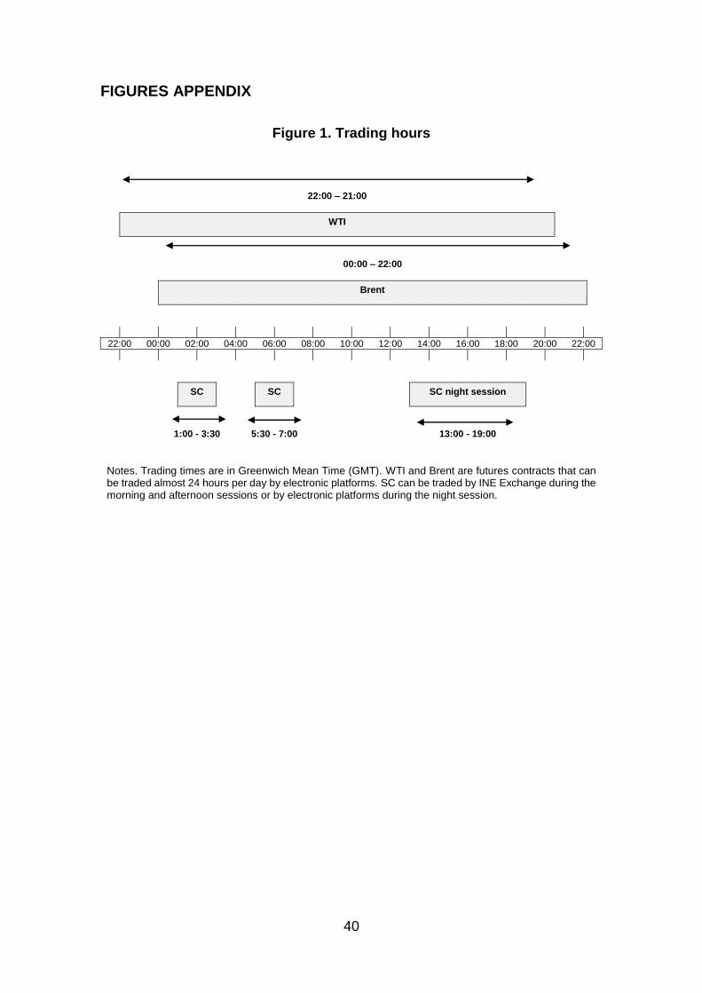
3.2. Trading hours

The three markets analysed have different trading schedules. This implies that

the knowledge and correct treatment of their trading hours is essential in order to

determine the methodology and to interpret the results obtained. Figure 1 shows

the diagram of trading hours. It is notable that the WTI and Brent futures contracts

are traded almost 24 hours per day. Firstly, WTI trading hours start at 22:00 and

go until 21:00 Greenwich Mean Time (GMT), with a one-hour break per day

between 21:00 and 22:00. Secondly, the Brent market starts its trading session

at 00:00 and goes until 22:00 (GMT). In contrast, the trading hours of the SC

market are less than the two previous markets. Officially, the trading hours of the

SC fluctuate between 1:00 - 3:30 and 5:30-7:00 (GMT). However, the INE, jointly

with SHFE, established a "night session" for all their products with the aim of

improving the internationalization of the market. This session runs from 13:00

until 19:00 (GMT). Therefore, the Chinese market has two differentiated periods

during the day. On the one hand, the morning-afternoon session, which has more

national investors and is expected to have more trading volume, and, on the other

hand, the overnight session, which could be more volatile and less liquid.

[Please Insert Figure 1]

Figure 2 exhibits daily settlement hours of SC, WTI and Brent for a day t. The

settlement price of SC is calculated at 7:00 (GMT), while WTI and Brent

coordinate the calculus of the settlement prices at the same time 18:30 (GMT).

However, ICE publishes two prices of Brent at 8:30 and 15:30 (GMT), named

15

Brent AM and Brent PM6 respectively, with the aim of coinciding with the release

of other OTC and standardised European energy benchmarks.


6 The Brent AM or Brent Crude Futures Singapore Minute Maker is calculated as a weighted average of trades done during a one minute period from 8:29 to 8:30 (GMT), while the Brent PM or Brent Crude Futures Minute Maker is calculated for each marker month as a weighted average of trades done during a one minute period from 15:29 to 15:30 (GMT). For more information of Brent AM and Brent PM please see www.theice.com.

16

4. DATA AND PRELIMINARY ANALYSIS

4.1. Data and summary statistics

The close prices transactions for all monthly deliveries were collected through

Thomson Reuters. For our analysis, we have decided to use the near-to-maturity

contract, as is usually the most liquid. Moreover, to generate the daily close prices

series, we have taken the close prices of the nearby contract up to five days

before its delivery. On this date, we have made the rollover to the next near-to-

maturity contract. The use of this criterion responds to the fact that the crude oil

market participants close positions in the front contract five days before its expiry

and, as a consequence, the liquidity passes to the next nearby contract. The

series of daily returns follow the same criterion, with the particularity that when

there is a change of contract, the returns of that day are calculated with the prices

of the same contract, in order to avoid artificial jumps in the return series.

Therefore, the prices and returns series have been calculated separately to take

into account the contract changes that take place during the entire sample period

and to not fall into the error of mixing different contract prices. Besides, we

calculate crude oil returns using the following relation: 𝑟𝑂𝐼𝐿,𝑡 = ln(𝑃𝑂𝐼𝐿,𝑡

𝑃𝑂𝐼𝐿,𝑡−1), where

𝑃𝑂𝐼𝐿,𝑡 is the -th price level at time t and where OIL is WTI, Brent or SC.

For our daily analysis, two sample periods have been considered. The first

sample has been used to analyse if the launch of SC has changed the

relationship between WTI and Brent. Daily settlement prices have been taken into

account and the sample covers the period from January 5, 2016 through May 9,

2019. In the second sample, the daily settlement prices and returns of the three

17

markets have been used to study the links among the three markets. This second

sample goes from March 26, 2018 to May 9, 2019.

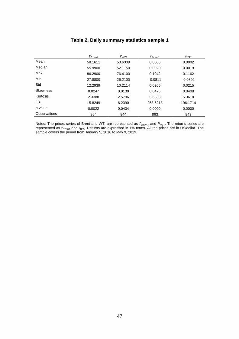
Table 2 and Table 3 show the summary statistics of both samples. The results of

table 2 show that, in the last three years, the mean of Brent prices have been

higher than WTI. Moreover, as we can see in Figure 3.A, during the 2016-2019

period the Brent prices have been above WTI. WTI is sweeter and lighter than

Brent, therefore, it is supposed to have a higher average price than Brent.

However, examining Table 3 and Figure 3.B, we notice that the SC contract have

also a higher price, during the sample period than WTI, being the Brent the most

expensive contract. Location, transporting cost and level production can help to

explain these crude oil prices differentials. The Brent is a seaborne oil grade

because is extracted from locations of UK coast and well connected to the global

trade routes. The warehouses of the SC are also connected to the coasts of

China. Nevertheless, the WTI must be transported from Cushing, Oklahoma, by

pipelines. These transporting differences are known as “location spread” and help

to explain the prices differences among the three contracts.



In addition, Table 2 and Table 3 show the results of the Jarque-Bera test. All the

variables taken into account in our study do not follow a normal distribution. In

addition, return series are leptokurtic, as the kurtosis is higher than the normal

distribution.


18

Figures 4.A, 4.B and 4.C show the daily returns for WTI, Brent and SC,

respectively. We can observe in the three series the following tendency: large

(small) changes in oil prices are followed by large (small) changes. This

phenomenon is known in the financial literature as volatility clustering and

provokes that the current volatility tends to be positively correlated with the

preceding level. It justifies the use of GARCH models that allow the conditional

variance to be dependent on past variances.

4.2. Preliminary analysis on volume and open interest

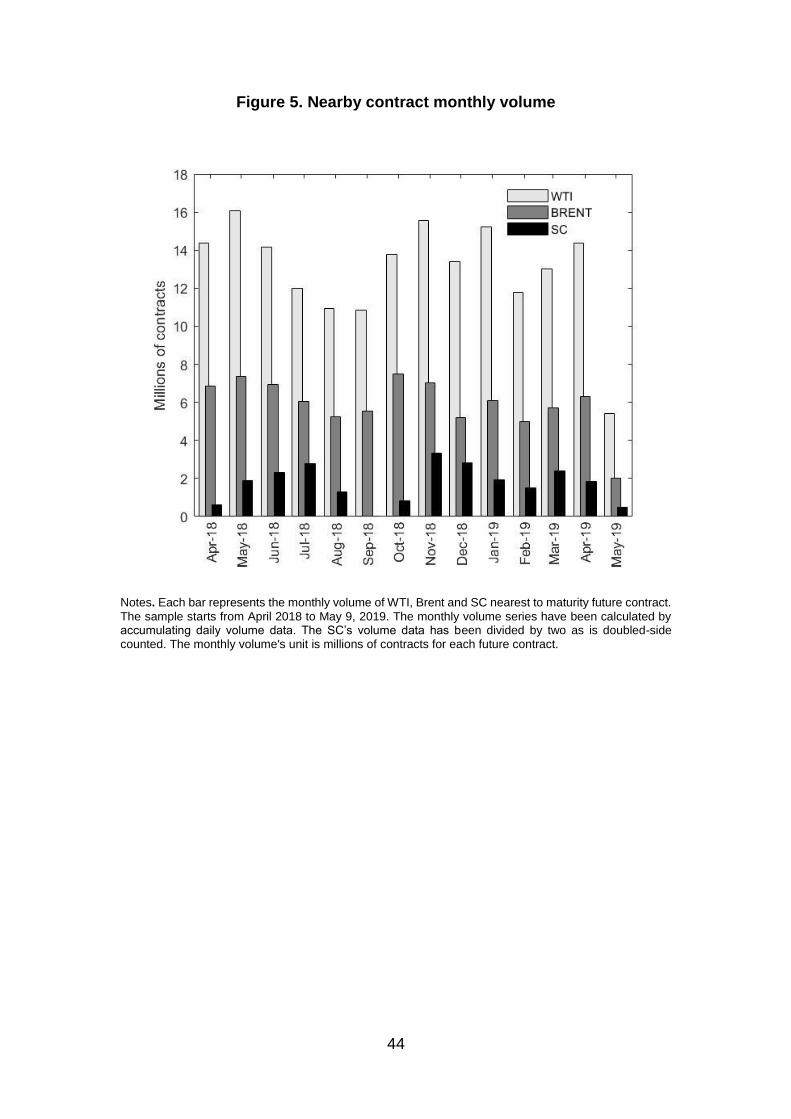
Figure 5 presents the monthly near-contract daily volume of the three contracts.

Sample period goes from April 2018 to May 2019. The WTI is the futures contract

with the highest monthly volume, followed by Brent. One remarkable fact of SC

nearest contract to maturity is the low monthly volume quoted in August and

September 2018. When the first SC futures contract was launched on March 26,

2018; the near-to-maturity contract was the one delivered at September 2018 and

the rest of the contracts were delivered monthly consecutively from October 2018

to March 2019. In August 2018, the daily trading volume of the near-maturity

contract (September 2018) began to drop, while the fourth maturity contract

increased in daily volume. As we have previously mentioned, both academia and

practitioners used to choose the nearest maturity futures contract for econometric

analysis because, usually, it has more trading volume and open interest.

Nevertheless, as we can notice in Figure 5 for the SC contract this assumption

does not perform. For this reason, testing commences by analysing the effects of

the listing of the SC futures contracts on total trading volume and open interest

data and not only for the nearby contract.

19


Table 4 reports the results for the mean and median of the daily trading volume

and open interest data for all the futures contracts traded at the same moment in

the three markets. Two periods have been differentiated: before and after the

launch of the SC futures contract that took place on March 26, 2018. The equality

of means has been checked with the F-test. However, given the absence of

normality in these samples, non-reported in the paper, the equality of medians

has been tested with the Kruskal-Wallis test. WTI and Brent total volume features

do not exhibit significant changes. The same issue is observed for Brent open

interest data. However, the WTI open interest has significantly increased, after

the introduction of the SC futures contract. Following Lucia and Pardo (2010), an

increase in the daily open interest data relative to the volume of trading indicates

that there is either a decrease in the activity of the speculators or an increase in

the activity of hedgers. Therefore, these preliminary results suggest that the

introduction of the SC futures contract has been accompanied by an increase in

the degree of hedging only in the WTI market.


20

5. METHODOLOGY

The purpose of this section is to describe the methods used in our empirical

analysis. The research is divided into two parts. Firstly, using daily synchronous

data, we analyse the relationship between Brent and WTI and the possible

influence of the SC in their long- and short-run dynamics. The second part of this

research is focused on the study of the links among the three markets, using

asynchronous daily data. In each analysis, we have used the data corresponding

to the days when the markets considered are simultaneously open.

5.1. VECM-BEKK

Firstly, we study the relationship between the two most important crude oil futures

contracts. Following previous studies on crude oil dynamics (Kaufmann and

Banerjee (2014) and Aruga (2015), among others), we analyse cointegration

between Brent and WTI. Cointegration is a helpful tool to examine if crude oil

prices in different markets move together. In fact, if we find a cointegration

relationship between Brent and WTI, it would be an argument for the globalization

hypothesis of the crude oil market.

To test cointegration, we first need to examine the integration order of the time

series. A variable 𝑦𝑡 is integrated of order 𝑑 (𝑦𝑡~𝐼(𝑑)) if it is necessary to

difference it 𝑑times for getting a stationary transformation and it has 𝑑unit roots.

The stationary of Brent and WTI log prices is examined by the augmented Dicky-

Fuller (ADF) test. The null hypothesis of the ADF test is that a unit root is present

in a time series sample. If we do not reject the ADF null hypothesis, log-price first

differences would be applied and we will test again the presence of unit roots in

the returns.

21

After testing the presence of unit roots, we will continue with the cointegration

analysis. Considering two time series 𝑦1,𝑡 and 𝑦2,𝑡, which both are𝐼(𝑑). In general,

any linear combination of 𝑦1,𝑡 and 𝑦2,𝑡 will be 𝐼(𝑑). Nevertheless, there is a vector

(1, −𝑏)′ such as the linear combination “𝑧 = 𝑦1,𝑡 − 𝑎 − 𝑏𝑦2,𝑡" is 𝐼(𝑑 − 𝑏), being

𝑑 ≥ 𝑏 > 0.

In order to test if Brent and WTI are cointegrated, we apply Johansen (1991)

tests. Johansen’s multivariate maximum likelihood approach is based on the

vector autoregressive model (VAR) of order p:

𝒚𝒕 = 𝝁𝒕 + 𝑨𝒊𝒚𝒕+. . . +𝑨𝒑𝒚𝒕−𝒑 + 𝑫𝑿𝒕 + 𝜺𝒕 (1)

where 𝒚𝒕 = {𝑦1,𝑡, 𝑦2,𝑡} = {𝑙𝑛(𝑃𝐵𝑅𝐸𝑁𝑇,𝑡), 𝑙𝑛(𝑃𝑊𝑇𝐼,𝑡)}~𝐼(1)∀𝑡 = 1,… , 𝑇; 𝑿𝒕 is a

vector of deterministic variables (linear time trends, dummies, etc…) and 휀𝑡 is the

vector of innovations.

The VAR (p) can be re-written as VECM (p-1) (Vector Error Correction Model):

∆𝒚𝒕 = 𝝁𝒕 + 𝝅𝒚𝒕−𝟏 + ∑ 𝜞𝒊∆𝒚𝒕−𝟏

𝒑−𝟏

𝒊=𝟏

+ 𝑫𝑿𝒕 + 𝜺𝒕 (2)

where

𝝅 = ∑𝑨𝒊 − 𝑰

𝒑

𝒊=𝟏

𝑎𝑛𝑑𝚪𝒊 = −∑𝑨𝒊

𝒑

𝒋=𝟏

The VAR (p) model is estimated by maximum likelihood. Then, the estimation of

the rank of the 𝝅 is analysed. If 𝑟𝑘(𝝅) = 1, Brent and WTI log prices are

cointegrated, there would exist 2x1 matrices 𝜶 and 𝜷, each with rank 1, such as

22

𝝅 = 𝜶𝜷′ and 𝜷′𝒚𝒕 is stationary. The elements of 𝜶 are the adjustment parameters

of the VECM and 𝜷 is the cointegrating vector.

Johansen (1991) proposed two tests for contrast the rank of the matrix 𝝅: the

trace and the maximum eigenvalue tests. The trace test contrasts the following

null hypothesis:

𝐻𝑜: 𝑅𝑎𝑛𝑘(𝜋) ≤ 𝑚

𝐻1: 𝑅𝑎𝑛𝑘(𝜋) > 𝑚

For test the cointegrating relationship between WTI and Brent log prices, we will

apply two tests with m=0 and m=1.

The trace test statistic is defined as:

𝐿𝑇𝑟(𝑚) = −𝑇 ∑ ln(1 − �̂�𝑖)

𝑘

𝑖=𝑚+1

(3)

where �̂�𝑖 are the generalized eigenvalues estimated for a given matrix arising in

the estimation process by Maximum eigenvalue.

The maximum eigenvalue tests the following null hypothesis:

𝐻𝑜: 𝑅𝑎𝑛𝑘(𝜋) = 𝑚

𝐻1: 𝑅𝑎𝑛𝑘(𝜋) = 𝑚 + 1

where the maximum eigenvalue statistic is defined as:

𝐿𝑚𝑎𝑥 =−𝑇ln(1 − �̂�𝑚+1) (4)

23

It is well-known that Johansen’s (1991) approach to cointegration is the most

popular technique for estimating long-run economic relationships. Nevertheless,

Ahking (2002) finds that the modelling of the deterministic components of the

cointegration equation has an important role in the power of Johansen’s test to

detect cointegration relationships. In some cases, the model miss-specification

can provoke misleading conclusions about the existence of cointegration.

Moreover, the number of observations can influence the power of the Johansen

test to detect cointegration. For this reason, we are going to check if oil log prices

are cointegrated by Engle and Granger (1987) and Phillips and Oularis (1990)

cointegration tests, apart from Johansen (1991) cointegration test

If there is a cointegration relationship between the variables, then we apply the

Granger and Engel representation theorem, which states that if two variables

{𝑦1,𝑡, 𝑦2,𝑡} are 𝐼(1) and are cointegrated,𝐶𝐼(1,1), then their dynamic relation is

characterized by a Vector Error Correction Model (VECM). The VECM represents

a long and short-run dynamic system in the joint behaviour of 𝑦1,𝑡 and 𝑦2,𝑡 over

time and takes the following form:

∆y1,t = 𝛼𝑦1 + ∑𝛿11∆y1,t−i

𝑚

𝑖=1

+ ∑𝛿12

𝑛

𝑖=1

∆y2,t−i + 𝛾𝑦1𝑧𝑡−1 + 휀𝑦1,𝑡 (5)

∆y2,t = 𝛼𝑦2 + ∑𝛿21∆y1,t−i

𝑝

𝑖=1

+ ∑δ22∆y2,t−i

𝑞

𝑖=1

+ 𝛾𝑦2𝑧𝑡−1 + 휀𝑦2,𝑡 (6)

휀𝑡 = (휀𝑦1,𝑡, 휀𝑦2,𝑡)′𝑖𝑖𝑑~𝑁(0, Σ)

∆ indicates the first-order time differences (i.e., ∆yt = 𝑦𝑡 − 𝑦𝑡−1). The variable 𝑧𝑡−1

is the lagged error correction term of the cointegration relationship between the

logarithms of Brent and WTI prices. 𝛾 is the speed of adjustment parameter and

24

high values will indicate a fast convergence rate toward equilibrium. Additionally,

to capture the effect of the SC futures launch in the dynamic relation, we have

introduced a dummy variable in the VECM, that is equal to 0 before March 26,

2018 and is equal to 1 after that date.

∆y1,t = 𝛼𝑦1 + ∑𝛿11∆y1,t−i

𝑚

𝑖=1

+ ∑𝛿12

𝑛

𝑖=1

∆y2,t−i + 𝛾𝑦1𝑧𝑡−1 + 𝑥1d + 휀𝑦1,𝑡 (7)

∆y2,t = 𝛼𝑦2 + ∑𝛿21∆y1,t−i

𝑝

𝑖=1

+ ∑δ22∆y2,t−i

𝑞

𝑖=1

+ 𝛾𝑦2𝑧𝑡−1 + 𝑥2d + 휀𝑦2,𝑡 (8)

휀𝑡 = (휀𝑦1,𝑡, 휀𝑦2,𝑡)′𝑖𝑖𝑑~𝑁(0, Σ)

Equations (9) to (12) have been estimated by Ordinary Least Squares. In addition

to the long- and short-run dynamics that are jointly governing Brent-WTI

relationship, we are interested in the volatility spillover transmission between both

markets. To study this phenomenon, we apply the BEKK approach proposed by

Engle and Kroner (1995). The residual series of both VECM models (equations

(9) – (12)) have been saved in order to use them as observable data to estimate

the BEKK models. Therefore, the VECM-BEKK models have been estimated by

two steps procedure, reducing in this way the number of parameters to estimate

and allowing faster convergence in the estimation procedure. The compact form

of the BEKK multivariate model is as follows:

𝜺𝒕 = 𝐮𝐭𝐇𝐭

𝟏𝟐𝑎𝑛𝑑𝒖𝒕 ∼ 𝑁(0,1)

𝑯𝒕 = 𝑪𝑪′ + 𝑨′𝜺𝒕−𝟏𝜺𝒕−𝟏′ 𝑨 + 𝑩′𝑯𝒕−𝟏𝑩 (9)

where 𝑯𝒕 is the conditional variance-covariance matrix in t, and 𝑪, 𝑨 and 𝑩 are

matrices of parameters to be estimated. 𝑪 is an upper-triangular positive definite

25

matrix; 𝑨 is a matrix that captures the effects of market news; matrix 𝑩

characterize the extends to which current levels of conditional variances are

related to past conditional variances, and 𝜺𝒕−𝟏 are the unexpected shock series

obtained from VECM estimation.

In the particular case of two assets, the extended form of BEKK-GARCH model

is:

[ℎ11,t ℎ12,t

ℎ21,t ℎ22,t] = [

𝑐11 0𝑐21 𝑐22

] [𝑐11 0𝑐21 𝑐22

]′

+ [𝑎11 𝑎12

𝑎21 𝑎22] [

휀1,𝑡−12 휀1,𝑡−1휀2,𝑡−1

휀1,𝑡−1휀2,𝑡−1 휀2,𝑡−12 ] [

𝑎11 𝑎12

𝑎21 𝑎22]′

+ [𝑏11 𝑏12

𝑏21 𝑏22] [

ℎ11,𝑡−1 ℎ12,𝑡−1

ℎ21,𝑡−1 ℎ22,𝑡−1] [

𝑏11 𝑏12

𝑏21 𝑏22]′

(10)

where, ℎ11,𝑡 and ℎ22,𝑡 are the conditional time-varying variances of Brent and WTI,

respectively. The elements ℎ12,𝑡 = ℎ21,𝑡 are the conditional covariance of Brent

and WTI.

In order to test the impact of the new Chinese crude oil futures contract, we have

introduced a dummy variable in the conditional variance matrix equation.

Following Bala and Takimoto (2017), we include the dummy variable in the BEKK

model as follows:

𝑯𝒕 = (𝑪 + 𝐕dt)′(𝑪 + 𝑽𝑑𝑡) + 𝑨′휀𝑡−1휀𝑡−1

′ 𝑨 + 𝑩′𝑯𝒕−𝟏𝑩 (11)

𝑤ℎ𝑒𝑟𝑒𝑑𝑡𝑖𝑠𝑎𝑑𝑢𝑚𝑚𝑦𝑣𝑎𝑟𝑖𝑎𝑏𝑙𝑒𝑡ℎ𝑎𝑡 {𝟎𝒊𝒇𝒕 < 𝝉∗𝟏𝒊𝒇𝒕 ≥ 𝝉∗

and𝝉∗ = 𝑺𝑪′𝒔𝒍𝒂𝒖𝒏𝒄𝒉

26

𝑽 is a lower triangular matrix. By including the dummy variable in this way, we

help to preserve the restriction of positive definitive matrix 𝑯𝒕 and we avoid the

imposition of higher long-run variance. If estimated parameters of V matrix are

positive and significant, it suggests that volatility after the launch of the SC is

bigger than the period prior to the launch of the SC.

The parameters of equations (13) and (15) are estimated by maximizing the

following likelihood function, assuming normally distributed errors:

𝑳(𝜽) = −𝑻𝒍𝒏(𝟐𝝅) −𝟏

𝟐∑𝒍𝒏|𝑯𝒕(𝜽)| + 𝜺𝒕′𝑯𝒕

−𝟏(𝜽)𝜺𝒕

𝑻

𝒕=𝟏

(12)

where T is the total sample number and 𝜽 represents the parameter vector to be

estimated. Numerical techniques have been used to minimize -𝑳(𝜽).

27

5.2. Multiple non-linear regression analysis

As we have described in Section 3, trading times of the three markets of our

interest do not perfectly overlap. Therefore, the non-simultaneity of trading times

for WTI, Brent and SC may affect the results of cross-correlations and

regressions with daily returns. Peiró et al. (1998) proposed a multiple regression

system that distinguishes between the influencing ability and the sensitivity of a

market to be influenced, solving the problem of non-simultaneity. On the one

hand, we have applied the model to Brent, WTI and SC futures contracts, taking

the official settlement prices both for Brent and WTI. Given the simultaneity of the

settlement prices of WTI and Brent, this equation system (A) has a purely

historical descriptive purpose:

𝑟𝑏𝑟𝑒𝑛𝑡,𝑡 = 𝛼𝑏𝑟𝑒𝑛𝑡 + 𝛽𝑤𝑡𝑖𝜆𝑏𝑟𝑒𝑛𝑡𝑟𝑤𝑡𝑖,𝑡 + 𝛽𝑠𝑐𝜆𝑏𝑟𝑒𝑛𝑡𝑟𝑠𝑐,𝑡 + 𝑢𝑏𝑟𝑒𝑛𝑡,𝑡 (13)

𝑟𝑤𝑡𝑖,𝑡 = 𝛼𝑤𝑡𝑖 + 𝛽𝑏𝑟𝑒𝑛𝑡𝜆𝑤𝑡𝑖𝑟𝑏𝑟𝑒𝑛𝑡,𝑡 + 𝛽𝑠𝑐𝜆𝑤𝑡𝑖𝑟𝑠𝑐,𝑡 + 𝑢𝑤𝑡𝑖,𝑡 (14)

𝑟𝑠𝑐,𝑡 = 𝛼𝑠𝑐 + 𝛽𝑏𝑟𝑒𝑛𝑡𝜆𝑠𝑐𝑟𝑏𝑟𝑒𝑛𝑡,𝑡−1 + 𝛽𝑤𝑡𝑖𝜆𝑠𝑐𝑟𝑤𝑡𝑖,𝑡−1 + 𝑢𝑠𝑐,𝑡 (15)

On the other hand, we have estimated another system (B) where the dependent

variables are Brent PM, WTI and SC. As we have shown in Figure 2, all these

variables are non-synchronous and, therefore, the prediction purpose with this

system would be possible:

𝑟𝐵𝑝𝑚,𝑡 = 𝛼𝐵𝑝𝑚 + 𝛽𝑤𝑡𝑖𝜆𝐵𝑝𝑚𝑟𝑤𝑡𝑖,𝑡−1 + 𝛽𝑠𝑐𝜆𝐵𝑝𝑚𝑟𝑠𝑐,𝑡 + 𝑢𝐵𝑝𝑚,𝑡 (16)

𝑟𝑤𝑡𝑖,𝑡 = 𝛼𝑤𝑡𝑖 + 𝛽𝐵𝑝𝑚𝜆𝑤𝑡𝑖𝑟𝐵𝑝𝑚,𝑡 + 𝛽𝑠𝑐𝜆𝑤𝑡𝑖𝑟𝑠𝑐,𝑡 + 𝑢𝑤𝑡𝑖,𝑡 (17)

𝑟𝑠𝑐,𝑡 = 𝛼𝑠𝑐 + 𝛽𝐵𝑝𝑚𝜆𝑠𝑐𝑟𝐵𝑝𝑚,𝑡−1 + 𝛽𝑤𝑡𝑖𝜆𝑠𝑐𝑟𝑤𝑡𝑖,𝑡−1 + 𝑢𝑠𝑐,𝑡 (18)

28

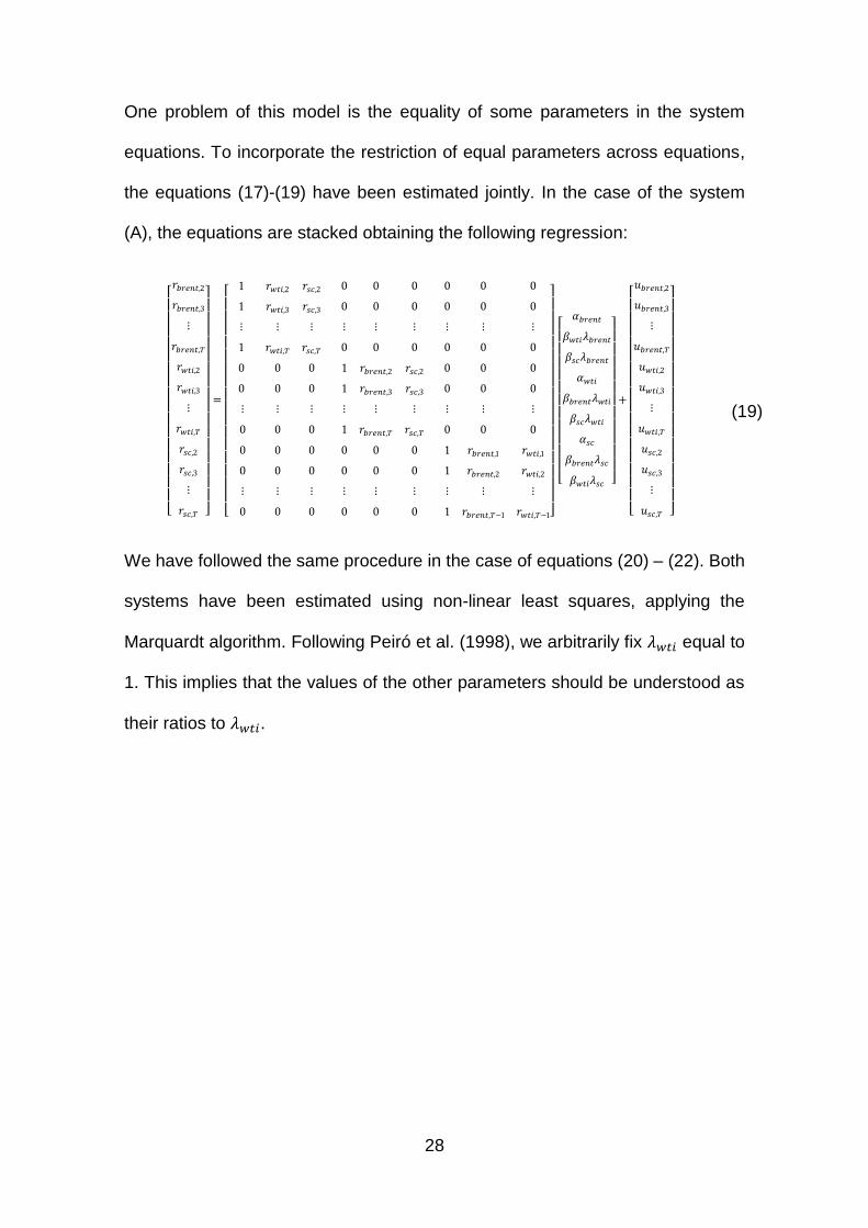
One problem of this model is the equality of some parameters in the system

equations. To incorporate the restriction of equal parameters across equations,

the equations (17)-(19) have been estimated jointly. In the case of the system

(A), the equations are stacked obtaining the following regression:

[ 𝑟𝑏𝑟𝑒𝑛𝑡,2

𝑟𝑏𝑟𝑒𝑛𝑡,3

⋮

𝑟𝑏𝑟𝑒𝑛𝑡,𝑇

𝑟𝑤𝑡𝑖,2

𝑟𝑤𝑡𝑖,3

⋮

𝑟𝑤𝑡𝑖,𝑇

𝑟𝑠𝑐,2

𝑟𝑠𝑐,3

⋮

𝑟𝑠𝑐,𝑇 ]

=

[ 1 𝑟𝑤𝑡𝑖,2 𝑟𝑠𝑐,2 0 0 0 0 0 0

1 𝑟𝑤𝑡𝑖,3 𝑟𝑠𝑐,3 0 0 0 0 0 0

⋮ ⋮ ⋮ ⋮ ⋮ ⋮ ⋮ ⋮ ⋮

1 𝑟𝑤𝑡𝑖,𝑇 𝑟𝑠𝑐,𝑇 0 0 0 0 0 0

0 0 0 1 𝑟𝑏𝑟𝑒𝑛𝑡,2 𝑟𝑠𝑐,2 0 0 0

0 0 0 1 𝑟𝑏𝑟𝑒𝑛𝑡,3 𝑟𝑠𝑐,3 0 0 0

⋮ ⋮ ⋮ ⋮ ⋮ ⋮ ⋮ ⋮ ⋮

0 0 0 1 𝑟𝑏𝑟𝑒𝑛𝑡,𝑇 𝑟𝑠𝑐,𝑇 0 0 0

0 0 0 0 0 0 1 𝑟𝑏𝑟𝑒𝑛𝑡,1 𝑟𝑤𝑡𝑖,1

0 0 0 0 0 0 1 𝑟𝑏𝑟𝑒𝑛𝑡,2 𝑟𝑤𝑡𝑖,2

⋮ ⋮ ⋮ ⋮ ⋮ ⋮ ⋮ ⋮ ⋮

0 0 0 0 0 0 1 𝑟𝑏𝑟𝑒𝑛𝑡,𝑇−1 𝑟𝑤𝑡𝑖,𝑇−1]

[

𝛼𝑏𝑟𝑒𝑛𝑡

𝛽𝑤𝑡𝑖𝜆𝑏𝑟𝑒𝑛𝑡

𝛽𝑠𝑐𝜆𝑏𝑟𝑒𝑛𝑡

𝛼𝑤𝑡𝑖

𝛽𝑏𝑟𝑒𝑛𝑡𝜆𝑤𝑡𝑖

𝛽𝑠𝑐𝜆𝑤𝑡𝑖

𝛼𝑠𝑐

𝛽𝑏𝑟𝑒𝑛𝑡𝜆𝑠𝑐

𝛽𝑤𝑡𝑖𝜆𝑠𝑐 ]

+

[ 𝑢𝑏𝑟𝑒𝑛𝑡,2

𝑢𝑏𝑟𝑒𝑛𝑡,3

⋮

𝑢𝑏𝑟𝑒𝑛𝑡,𝑇

𝑢𝑤𝑡𝑖,2

𝑢𝑤𝑡𝑖,3

⋮

𝑢𝑤𝑡𝑖,𝑇

𝑢𝑠𝑐,2

𝑢𝑠𝑐,3

⋮

𝑢𝑠𝑐,𝑇 ]

(19)

We have followed the same procedure in the case of equations (20) – (22). Both

systems have been estimated using non-linear least squares, applying the

Marquardt algorithm. Following Peiró et al. (1998), we arbitrarily fix 𝜆𝑤𝑡𝑖 equal to

1. This implies that the values of the other parameters should be understood as

their ratios to 𝜆𝑤𝑡𝑖.

29

6. RESULTS AND DISCUSSION

6.1. VECM-BEKK results

Table 3 provides the results of the ADF test. The outcome of the ADF test

indicates that the log prices of Brent and WTI contain a unit root at the 1% level.

Therefore, log prices are not stationary. In the case of the first order differences,

the null hypothesis is rejected at the 1% level, confirming that the first order

differences of the log prices are stationary.


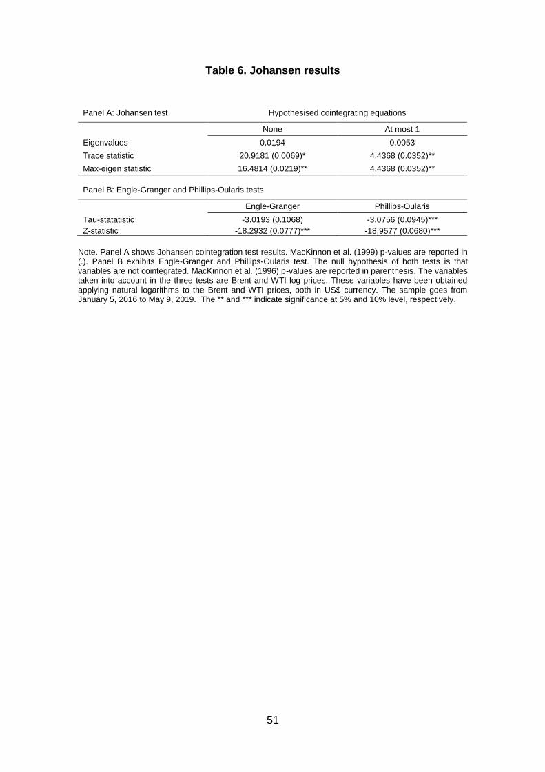
Table 4 (Panel A) shows Johansen Cointegration test results. The trace statistic

indicates that the π matrix has full rank (r=2) at the 10% significance level. This

contradictory result reveals a low power of the Johansen Cointegration test to

detect the presence of a cointegrating relationship among the variables.

Furthermore, the Maximum eigenvalue statistic result is that Brent and WTI log

prices are not cointegrated. Conversely, the results of Engle-Granger and Philips-

Oularis cointegration tests, that are shown in Table 4 (Panel B), indicate that

Brent and WTI log prices are cointegrated at the 10% significance level. Given

these results, we continue the study investigating the short- and long-run

causality by the estimation of the VECM model.


Table 5 shows the estimation results of the VECM without and with SC dummy

variable. Qualitatively, the results of both models are similar. The short-run

transmission parameters are not significant at any level. The Brent’s speed of

adjustment parameter is not statically significant and the WTI’s adjustment

30

parameter is positive and significant at the 5% level. During the period 2017-

2019, Brent prices have been above WTI prices. Therefore, WTI prices need to

rise to restore equilibrium. The statically significance of the WTI’s adjustment

parameter respects to Brent’s adjustment parameter indicates that Brent leads

WTI in the long-run.

The dummy parameters estimated, that have been included in equations (11) and

(12), are significant and negative at the 1% level only in the case of the WTI

equation. This parameter is directly affecting the intercept term of WTI equation.

The negative value of the dummy parameter suggests that the unconditional

mean of WTI has been reduced since the launch of the new Chinese futures

contract. Nevertheless, there are factors that could be affecting this result, such

as the Organization of Petroleum Exporting Countries (OPEC) events that took

place during the 2018 year.

Another relevant result is the change in the values of the speed of adjustment

parameters in the VECM with dummy variable respects to the VECM without

dummy variable. The WTI adjustment parameter has increased. Therefore, the

launch of SC has strengthened the leadership of Brent on WTI. Table 5 (Panel

B) exhibits diagnostic tests of both VECM models. Akaike and Schwarz's

criterions present closest values for both models.


Table 8 shows the results of BEKK-GARCH estimation. Panel A.1 in Table 8

exhibits estimations of equation (14) and panel A.2 in Table 8 shows the

estimations of equation (15). The results indicate that the volatilities of WTI and

Brent are affected by their own past shocks and volatilities. Moreover, the cross-

31

market effects are statistically significant at the 1% level in either direction,

indicating a bi-directional volatility spillover among both markets. In addition, the

estimations of the dummy parameters are negative and significant at the 1%

level. The launch of the SC has reduced the long-run variance of Brent and WTI.

Therefore, the volatility transmission patterns have changed since the launch of

SC.


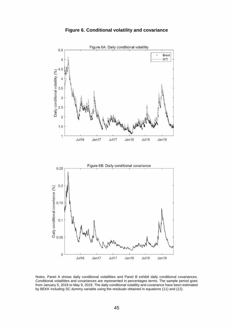
Figure 6 (A) shows the daily conditional volatility and covariance for BEKK

including SC dummy variable. Both volatility series have similar patterns, but the

conditional volatility of WTI is above Brent during all period. Moreover, Figure 6

(B) exhibits conditional covariance time-varying. Figure 6 shows a drop on

conditional volatilities and covariance in June 2016, this date coincides with the

OPEC meeting in Vienna. On June 2, 2016 crude oil prices suffered a drop as a

response to the OPEC meeting on that date, when oil ministers ended the

meeting reaching any kind of consensus on regulating the price and supply of

crude oil.

Moreover, conditional volatilities and covariance increased during December

2018 and January 2019. This increase can be explained by the fact that in

December 2018 monthly U.S crude oil production reached 11.96 million b/d, the

highest monthly level of crude oil production in U.S history. The U.S. historical

production levels on December 2018 has resulted in low crude oil prices and high

conditional volatilities and covariances during December 2018 and January 2019.


32

6.2. Multiple non-linear regression results

Table 9 reports crossed correlations between the returns of WTI, Brent, Brent PM

and SC. Given the absence of normality in the returns, we have used Kendall’s

tau correlation coefficient, that is one descriptive measure of association in a

bivariate sample. The Tau-test is a nonparametric test that tests the null

hypothesis of independence between two series. Panel A in Table 9 shows

contemporaneous daily returns cross-correlations. The returns of WTI are high

and positively correlated at the 1% level with the returns of Brent and Brent PM.

In addition, returns of Brent PM are positively correlated at the 5% level with SC’s

returns. Panel B in Table 9 reports a similar analysis between the OIL returns and

the OIL returns lagged one period. In this case, 𝑟𝑊𝑇𝐼,𝑡 and 𝑟𝐵𝑅𝐸𝑁𝑇,𝑡 are negatively

correlated at the 10% level with 𝑟𝑊𝑇𝐼,𝑡−1 and 𝑟𝐵𝑅𝐸𝑁𝑇,𝑡−1. The correlation between

𝑟𝑆𝐶,𝑡 and the returns of WTI, Brent and Brent PM lagged one period is positive

and significant at the 1% level.

The trading times may help to explain the cross-correlation results. As we have

previously mentioned, SC settlement time is at 7:00 (GMT), whilst Brent and WTI

report settlement prices at 18:30 (GMT). Moreover, the settlement time of Brent

PM is at 15:30 (GMT). Therefore, it makes sense that returns on the day 𝑡 − 1 of

WTI, Brent and Brent PM are correlated with the SC’s returns on day 𝑡. These

results indicate that a model that tries to explain OIL returns should take into

account not only contemporaneous information but also past information about

OIL returns.

Furthermore, it is remarkable that the highest correlation is observed between

contemporaneous returns of WTI and Brent on day 𝑡. The settlement times of

33

WTI and Brent coincide at 18:30 (GMT). If there exist global innovations in the

OIL market, the relationship between two variables should be higher the longer

the overlapping between their trading times. Hence, the overlapping of trading

times could be an explanation of the high correlation observed on day 𝑡between

WTI-Brent returns pairs. The feature that Brent and WTI are futures contracts that

can be traded almost 24 hours during the day could enlighten this event. It opens

the discussion about the usefulness of analysing daily returns in markets that can

be traded continuously by electronic platforms, as is the case of WTI and Brent

futures contracts.

The SC contract is not contemporaneous correlated with Brent and WTI. This

cross-correlations result indicates that SC may is not influencing WTI and Brent

markets. We will conduct a more detailed analysis of the links between the three

markets to clarify these empirical results.


Table 10 shows the joint estimation of systems A and B. Panel A in Table 10

exhibits the joint estimation of equations (17), (18) and (19). In this system, only

the parameters �̂�𝐵𝑅𝐸𝑁𝑇 and 𝜆𝑆𝐶 are significant at the 1% level. We are interested

in the relative values of these parameters to 𝜆𝑆𝐶 = 1. These results indicate that

Brent is the only influential market, since its beta is positive and significant at the

1% level and the betas of WTI and SC are not significant at any significance level.

WTI is the most sensitive market, as its ability to be influenced compared to SC

is higher. Moreover, Brent market appears as an insensitive market.

Panel B in Table 10 shows the joint estimation of equations (20), (21) and (22).

The significant parameters of system B are similar to the estimation of system A.

34

Nevertheless, the influential capacity of Brent PM is lower than the estimation of

the influential capacity of Brent. In the case of the SC ability to be influenced, the

estimation output of System B is higher than the results of System A. These

results are consistent with the previous cross-correlation analysis and our

hypothesis that the three markets are related in a contemporaneous and non-

contemporaneous way, depending on their trading times.


35

7. SUMMARY AND CONCLUDING REMARKS

This paper investigates two main questions. Firstly, testing if the launch of SC

futures contract has been accompanied by a change in the relationship between

the two main crude oil benchmarks, Brent and WTI. Secondly, the information

flows among the three futures markets: Brent, WTI and SC. These objectives are

framed within a common theme: the globalization of the crude oil market.

Since the launch of the SC contract, there has been speculation about the impact

of the SC on Brent and WTI markets. In a first analysis of the total volume and

open interest of Brent and WTI, we have observed that the trading of SC contracts

has been accompanied by a significant increase in the open interest of WTI

market. In addition, we have analysed the impact of the SC on the short- and

long-term relationship between Brent and WTI markets by including a dummy

variable in the VECM model. Firstly, similar to previous studies, we conclude that

Brent and WTI share a common tendency in the long-run. Moreover, our findings

suggest that Brent leads WTI in the long-run and the launch of the SC has

accompanied by the strengthening of the leadership of Brent on WTI. Secondly,

our findings suggest that there is no causal relationship between both oils in the

short-run. Therefore, the oil market is integrated, at least between the two main

benchmarks. To investigate the integration hypothesis, further research could be

an intraday cointegration analysis, including another crude oil futures contract

such as the SC.

Additionally, we have performed a volatility analysis between the two benchmarks

by applying a BEKK model. The results indicate that short-term volatility

relationship between both markets is explained by the volatility spillover between

36

WTI and Brent markets. Furthermore, we showed that since the launch of the SC

contract, the long-term variance and covariance of both markets have been

reduced.

Regarding the results of the analysis of the market linkages among the three

markets, our findings indicate that Brent is the most influential market, while SC

appears as the most sensitive. In addition, the SC contract has no influence on

WTI and Brent daily prices. Therefore, the leadership of the Brent-WTI oil futures

market is not threatened yet.

Given the high degree of overlap between the trading times among the main oil

futures benchmarks, we highlight the importance of studying the information flows

between international markets by models such as Peiró et al. (1998) or by an

intraday analysis. Moreover, our results are of interest to practitioners and

individual investors as the knowledge of which crude oil futures contract is

exercising leadership in the crude oil market is important to take positions in crude

oil futures and get gains in price and time.

37

REFERENCES

Adelman, M. A. (1984). “International Oil agreement.” International association

for Energy Economics 5(3): 1-9.

Ahking, F. W. (2002). "Model Mis-Specification and Johansen's Co-Integration

Analysis: An Application To The US Money Demand". Journal Of

Macroeconomics 24 (1): 51-66.

Aruga, K. (2015). “Testing the International Crude Oil Market Integration with

Structural Breaks.” Economics Bulletin 35(1): 641-649.

Bala, D. A., and Takimoto T. 2017. "Stock Markets Volatility Spillovers During

Financial Crises: A DCC-MGARCH With Skewed- T Density Approach". Borsa

Istanbul Review 17 (1): 25-48.

Bhar, R., Hammoudeh, S. and Thompson, M. (2008). “Component structure for

nonstationary time series: Application to benchmark oil prices”. International

Review of Financial Analysis 17(5): 971-983.

Candelon, B., Joëts, M. and Tokpavi, S. (2013). “Testing for Granger causality in

distribution tails: An application to oil markets integration.” Economic Modelling

31: 276-285.

Fattouh, B. (2010). “The dynamics of crude oil price differentials.” Energy

Economics 32(2): 334-342.

Engle, R.F. and C.W.J. Granger (1987) "Co-integration and Error Correction:

Representation, Estimation, and Testing". Econometrica 55(2): 251-276.

38

Engle, R. F. and Kroner, K. F. (1995). “Multivariate Simultaneous Generalized

ARCH.” Econometric Theory 11(1): 122-150.

Giulietti, M., Iregui, A. and Otero, J. (2014). “Crude oil price differentials, product

heterogeneity and institutional arrangements”. Energy Economics 46: 28-32.

Kaufmann, R. and Banerjee, S. (2014). “A unified world oil market: Regions in

physical, economic, geographic, and political space.” Energy Policy 74: 235-242.

Klein, T. (2018). “Trends and contagion in WTI and Brent crude oil spot and

futures markets - The role of OPEC in the last decade”. Energy Economics 75:

636-646.

Ji, Q. and Fan, Y. (2015). “Dynamic integration of world oil prices: a

reinvestigation of globalisation vs. regionalisation.” Applied Energy 155: 171-180.

Johansen, S. (1991). “Estimation and hypothesis testing of cointegration vectors

in Gaussian vector autoregressive models”. Econometrica 59(6): 1551-1580.

Lucia, J. J., and Pardo, A. (2010). “On measuring speculative and hedging

activities in futures markets from volume and open interest data.” Applied

Economics, 42(12): 1549-1557.

MacKinnon, J. G., Haug, A. A. and Michelis, L. (1998). “Numerical distribution

functions of Likelihood Ratio Test for Cointegration”. Department of Economics,

University of Canterbury.

Milonas, N. and Henker, T. (2001). “Price spread and convenience yield

behaviour in the international oil market.” Applied Financial Economics 11(1): 23-

36.

39

Peiró, A., Quesada J. and Uriel E. (1998) “Transmission of movements in stock

markets.” The European Journal of Finance 4(4): 331-343.

Phillips, P. and Ouliaris, S. (1990). "Asymptotic Properties of Residual Based

Tests for Cointegration". Econometrica 58 (1): 165–193.

Reboredo, J. (2011). “How do crude oil prices co-move? a copula approach.”

Energy Economics 33(5): 948-955.

Weiner, R. (1991). “Is the World Oil Market “One great pool”?”. The Energy

Journal 12(3): 95-107.

Zhang, J. and Umehara, N. (2019). “How far is Shanghai INE Crude Oil Futures

from an International Benchmark in Oil Pricing?”. Institute for International

Monetary Affairs (4, 2019)

40

FIGURES APPENDIX

Figure 1. Trading hours

22:00 – 21:00

WTI

00:00 – 22:00

Brent

22:00 00:00 02:00 04:00 06:00 08:00 10:00 12:00 14:00 16:00 18:00 20:00 22:00

SC SC SC night session

1:00 - 3:30 5:30 - 7:00

13:00 - 19:00

Notes. Trading times are in Greenwich Mean Time (GMT). WTI and Brent are futures contracts that can be traded almost 24 hours per day by electronic platforms. SC can be traded by INE Exchange during the morning and afternoon sessions or by electronic platforms during the night session.

41

Figure 2. Settlement times

SC (7:00) Brent PM (13:30) Brent (18:30)

6:00 7:00 8:00 9:00 10:00 11:00 12:00 13:00 14:00 15:00 16:00 17:00 18:00 19:00

WTI (18:30)

Notes. Settlement times are in Greenwich Mean Time (GMT).

42

Figure 3. Daily prices

Notes. Figure 3A shows WTI and Brent daily prices for the period of January 5, 2016 to May 9, 2019. In Figure 3B, WTI, Brent and SC daily prices are plotted and covers the period from March 26, 2018 to May 2019. The prices series are in US$.

43

Figure 4. Daily returns

Notes. WTI, Brent and SC daily returns are plotted. Returns are represented in percentages terms. The sample period of Brent and WTI daily returns goes from January 2016 to May 2019. The sample period of SC daily returns goes from March 27, 2018 to May 9, 2019.May 9, 2019.

44

Figure 5. Nearby contract monthly volume

Notes. Each bar represents the monthly volume of WTI, Brent and SC nearest to maturity future contract.

The sample starts from April 2018 to May 9, 2019. The monthly volume series have been calculated by accumulating daily volume data. The SC’s volume data has been divided by two as is doubled-side counted. The monthly volume's unit is millions of contracts for each future contract.

45

Figure 6. Conditional volatility and covariance

Notes. Panel A shows daily conditional volatilities and Panel B exhibit daily conditional covariances. Conditional volatilities and covariances are represented in percentages terms. The sample period goes from January 5, 2016 to May 9, 2019. The daily conditional volatility and covariance have been estimated by BEKK including SC dummy variable using the residuals obtained in equations (11) and (12).

46

TABLES APPENDIX

Table 1. WTI, Brent and SC contract specifications

WTI Brent SC

Market NYMEX (New York

Mercantile Exchange)

ICE (InterContinental

Exchange)

INE (Shanghai

International Exchange)

Region United States Northwest Europe China

Barrels per contract Unit 1,000 1,000 1,000

Sulphur Content 0.24 % 0.42 % 1.5 %

API grades 39.6º 38.1º 32.0º

Contract Months Monthly contracts listed

for the current year and

the next 8 calendar

years and 2 additional

consecutive contract

months

Up to 96 consecutive

months

Monthly contracts of

recent twelve

consecutive months

followed by eight

quarterly contracts

Price quotation U.S. dollars and cents

per barrel

U.S. dollars and cents

per barrel

Yuan per barrel

Minimum price fluctuation $ 0.01 per barrel $ 0.01 per barrel ¥ 0.1 per barrel

Daily price limits 7% in each trading

session

None ± 4% from the

settlement price of the

previous day

Last trading day Three business day

before the twenty-fifth

calendar day of the

month prior to the

contract month. If the

twenty-fifth calendar

day is not a business

day, trading terminates

3 business day prior to

the business day

preceding the twenty-

fifth calendar day

The last trading day of

the month prior to the

delivery month

The last trading day of

the month prior to the

delivery month

Delivery period Delivery shall take place

no earlier than the first

calendar day of the

delivery month and no

later than the last

calendar day of the

delivery month

Stablished by EFP and,

in case of the cash

settlement, the next

trading day following the

last trading day for the

contract month.

Five consecutive

trading days after the

last trading day

Settlement Method Physical delivery EFP with an option to

cash settle against the

ICE Brent Index price

Physical delivery

Product code CL B SC

Data source: www.cmegroup.com www.theice.com www.ine.cn

47

Table 2. Daily summary statistics sample 1

𝑃𝐵𝑟𝑒𝑛𝑡 𝑃𝑊𝑇𝐼 𝑟𝐵𝑟𝑒𝑛𝑡 𝑟𝑊𝑇𝐼

Mean 58.1611 53.6339 0.0006 0.0002

Median 55.9900 52.1150 0.0020 0.0019

Max 86.2900 76.4100 0.1042 0.1162

Min 27.8800 26.2100 -0.0811 -0.0802

Std 12.2939 10.2114 0.0206 0.0215

Skewness 0.0247 0.0130 0.0476 0.0408

Kurtosis 2.3388 2.5796 5.6536 5.3618

JB 15.8249 6.2390 253.5218 196.1714

p-value 0.0022 0.0434 0.0000 0.0000

Observations 864 844 863 843

Notes. The prices series of Brent and WTI are represented as 𝑃𝐵𝑟𝑒𝑛𝑡 and 𝑃𝑊𝑇𝐼. The returns series are

represented as 𝑟𝐵𝑟𝑒𝑛𝑡 and 𝑟𝑊𝑇𝐼 .Returns are expressed in 1% terms. All the prices are in US/dollar. The

sample covers the period from January 5, 2016 to May 9, 2019.

48

Table 3. Daily summary statistics sample 2

𝑃𝐵𝑟𝑒𝑛𝑡 𝑃𝑊𝑇𝐼 𝑃𝑆𝐶 𝑟𝐵𝑟𝑒𝑛𝑡 𝑟𝑊𝑇𝐼 𝑟𝑆𝐶

Mean 70.8725 63.0313 69.9113 0.0001 -0.0002 0.0001

Median 72.1300 65.2500 70.8718 0.0020 0.0021 0.0012

Max 86.2900 76.4100 84.4568 0.0757 0.0832 0.0442

Min 50.7700 42.5300 52.4879 -0.0718 -0.0802 -0.0479

Std 7.1730 7.6100 6.1531 0.0183 0.0198 0.0155

Skewness -0.4505 -0.5809 -0.3138 -0.8122 -0.6829 -0.2004

Kurtosis 2.5842 2.3479 2.9303 6.1243 6.0826 3.7043

JB 12.0642 20.7539 4.5428 149.3213 134.0420 7.4152

p-value 0.0024 0.0000 0.1032 0.0000 0.0000 0.0245

Observations 290 284 272 289 283 271

Notes. The prices series of Brent, WTI and SC are represented as 𝑃𝐵𝑟𝑒𝑛𝑡, 𝑃𝑊𝑇𝐼 and 𝑃𝑆𝐶. The returns series

are represented as 𝑟𝐵𝑟𝑒𝑛𝑡, 𝑟𝑊𝑇𝐼 and 𝑟𝑆𝐶. Returns are expressed in 1% terms. All the prices are in US/dollar.

The sample covers the period from March 26, 2018 to May 9, 2019.

49

Table 4. Daily trading volume and open interest

Volume Open Interest

WTI Brent WTI Brent

From 4 January 2016 to 23 March 2018

Mean 1183684 841795 2096316 2307936

Median 1157999 835971 2135534 2311180

From 26 March 2018 to 9 May 2019

Mean 1192424 839101.3 2234658 2310569

Median 1169334 826742 2197986 2276531

Equality Tests

F-test 0.1564 0.0275 49.3317 0.0771

p-value 0.6926 0.8684 0.0000 0.7814

Kruskal-Wallis test 0.6292 0.0083 37.1275 0.7226

p-value 0.4277 0.9273 0.0000 0.3953

Notes. This table reports the mean and the median of the sum of the total daily trading volume and open interest of all the WTI and Brent futures contract. The first period goes from January 4, 2016 to March 23, 2018 and the second one runs from March 26, 2018 to May 9, 2019. The F statistic tests the null hypothesis of equality of means. Kruskal–Wallis statistic is the non-parametric equivalent of the F test and is distributed as a χ2 with one degree of freedom. All the p-values appear below the corresponding statistics. Daily trading volume and open interest are expressed in the number of contracts.

50

Table 5. Augmented Dickey-fuller unit roots test

Brent WTI

Level series -2.2390 -2.3604

(0.1926) (0.1535)

First order differences -20.034 -19.8033

(0.0000) (0.0000)

Note. Augmented Dickey-fuller test is used to examine the stationarity of the series. First-row test level series by using the log prices of the WTI and Brent. In the second row, the ADF test for first-order differences is analysed. Numbers in parenthesis indicate p-values. The number of lags has selected by the Akaike criterion. The sample goes from January 5, 2016 to May 9, 2019 for both futures contracts.

51

Table 6. Johansen results

Panel A: Johansen test Hypothesised cointegrating equations

None At most 1

Eigenvalues 0.0194 0.0053

Trace statistic 20.9181 (0.0069)* 4.4368 (0.0352)**

Max-eigen statistic 16.4814 (0.0219)** 4.4368 (0.0352)**

Panel B: Engle-Granger and Phillips-Oularis tests

Engle-Granger Phillips-Oularis

Tau-statatistic -3.0193 (0.1068) -3.0756 (0.0945)***

Z-statistic -18.2932 (0.0777)*** -18.9577 (0.0680)***

Note. Panel A shows Johansen cointegration test results. MacKinnon et al. (1999) p-values are reported in (.). Panel B exhibits Engle-Granger and Phillips-Oularis test. The null hypothesis of both tests is that variables are not cointegrated. MacKinnon et al. (1996) p-values are reported in parenthesis. The variables taken into account in the three tests are Brent and WTI log prices. These variables have been obtained applying natural logarithms to the Brent and WTI prices, both in US$ currency. The sample goes from January 5, 2016 to May 9, 2019. The ** and *** indicate significance at 5% and 10% level, respectively.

52

Table 7. VECM results

Panel A: VECM estimation

Model 1

∆y1,t = 𝛼𝑦1 + ∑𝛿11∆y1,t−i

𝑚

𝑖=1

+ ∑𝛿12

𝑛

𝑖=1

∆y2,t−i + 𝛾𝑦1𝑧𝑡−1 + 휀𝑦1,𝑡

∆y2,t = 𝛼𝑦2 + ∑𝛿21∆y1,t−i

𝑝

𝑖=1

+ ∑δ22∆y2,t−i

𝑞

𝑖=1

+ 𝛾𝑦2𝑧𝑡−1 + 휀𝑦2,𝑡

Brent

𝛼𝐵𝑟𝑒𝑛𝑡 𝛿11 𝛿12 𝛾𝐵𝑟𝑒𝑛𝑡

0.0009 -0.0917 -0.0065 0.0258

[1.3185] [-0.9081] [-0.0680] [1.5498]

WTI

𝛼𝑊𝑇𝐼 𝛿21 𝛿22 𝛾𝑊𝑇𝐼

0.0007 -0.1234 0.0457 0.0432**

[1.0394] [-1.1569] [0.4511] [2.4570]

Model 2

∆y1,t = 𝛼𝑦1 + ∑𝛿11∆y1,t−i

𝑚

𝑖=1

+ ∑𝛿12

𝑛

𝑖=1

∆y2,t−i + 𝛾𝑦1𝑧𝑡−1 + 𝑥1𝑑 + 휀𝑦1,𝑡

∆y2,t = 𝛼𝑦2 + ∑𝛿21∆y1,t−i

𝑝

𝑖=1

+ ∑δ22∆y2,t−i

𝑞

𝑖=1

+ 𝛾𝑦2𝑧𝑡−1 + 𝑥2𝑑 + 휀𝑦2,𝑡

Brent

𝛼𝐵𝑟𝑒𝑛𝑡 𝛿11 𝛿12 𝛾𝐵𝑟𝑒𝑛𝑡 𝑥1

0.0017*** -0.0857 -0.0151 0.0172 -0.0024

[1.7799] [-0.8456] [-0.1579] [0.7499] [-1.2002]

WTI

𝛼𝑊𝑇𝐼 𝛿21 𝛿22 𝛾𝑊𝑇𝐼 𝑥2

0.0022** -0.1236 0.0415 0.0500** -0.0044**

[2.1997] [-1.1557] [0.4094] [2.0606] [-2.0915]

Panel B: Diagnostic test

Model 1 R-sq. Adj. R-sq. Akaike Schwarz SC

Brent 0.0129 0.0129 -4.9309 -4.9084

WTI 0.0093 0.0094 -4.8229 -4.8004

Model 2 R-sq. Adj. R-sq. Akaike Schwarz SC

Brent 0.0117 0.0119 -4.9274 -4.8992

WTI 0.0070 0.0072 -4.8195 -4.7914

Note. Panel A shows estimations of equations (9)-(12). T-statistics are shown in brackets below each parameter estimation. The *, ** and *** indicates significance at 1%, 5% and 10% level, respectively. Panel B shows diagnostic tests. Sample cover the period from January 5, 2016 to May 9, 2019.

53

Table 8. BEKK results

Panel A: BEKK estimation

Panel A.1: BEKK without dummy variable

Panel A.2: BEKK with dummy variable

𝒄𝟏𝟏 0.0057 0.0007

(0.0000)* (0.0000)*

𝒄𝟐𝟏 0.0057 0.0014 (0.0000)* (0.0000)*

𝒄𝟐𝟐 0.0018 0.0013 (0.0000)* (0.0000)*

𝛂𝟏𝟏 0.0200 0.0151 (0.0000)* (0.0000)*

𝛂𝟏𝟐 0.0134 0.2512 (0.0000)* (0.0000)*

𝛂𝟐𝟏 0.0110 0.2201 (0.0000)* (0.0000)*

𝛂𝟐𝟐 0.0200 0.0183 (0.0000)* (0.0000)*

𝛃𝟏𝟏 0.9500 0.9714 (0.0000)* (0.0000)*

𝛃𝟏𝟐 0.0368 0.0099 (0.0000)* (0.0000)*

𝛃𝟐𝟏 0.0050 -0.0037 (0.0000)* (0.0003)*

𝛃𝟐𝟐 0.9499 0.9574 (0.0000)* (0.0000)*

𝒗𝟏𝟏 -0.0016 (0.0000)*

𝒗𝟐𝟏 -0.0029 (0.0000)*

𝒗𝟐𝟐 -0.0035

(0.0000)*

Akaike -14500.84 -10487.1398

Notes. Panel A.1. shows estimations of equation (13), while Panel A.2. exhibit estimations of equation (15). The sample covers the period from January 5, 2016 to May 9, 2019. The p-values are shown in parenthesis below each parameter estimation. The * indicates significance at the 1% level.

54

Table 9. Cross-correlation analysis

Panel A: contemporaneous analysis

𝑟𝑊𝑇𝐼,𝑡 𝑟𝐵𝑅𝐸𝑁𝑇,𝑡 𝑟𝐵𝑅𝐸𝑁𝑇𝑃𝑀,𝑡 𝑟𝑆𝐶,𝑡

𝑟𝑊𝑇𝐼,𝑡 1.0000

- 𝑟𝐵𝑅𝐸𝑁𝑇,𝑡 0.7350 1.0000

(0.0000)* - 𝑟𝐵𝑅𝐸𝑁𝑇𝑃𝑀,𝑡 0.4715 0.5359 1.0000

(0.0000)* (0.0000)* - 𝑟𝑆𝐶,𝑇 0.0398 0.0086 0.0895 1.0000

(0.3374) (0.8368) (0.0309)** -

Panel B: non-contemporaneous analysis

𝑟𝑊𝑇𝐼,𝑡 𝑟𝐵𝑅𝐸𝑁𝑇,𝑡 𝑟𝐵𝑅𝐸𝑁𝑇𝑃𝑀,𝑡 𝑟𝑆𝐶,𝑡

𝑟𝑊𝑇𝐼,𝑡−1 -0.0736 -0.0723 0.0632 0.4174

(0.0767)*** (0.0818)*** (0.1286) (0.0000)* 𝑟𝐵𝑅𝐸𝑁𝑇,𝑡−1 -0.0725 -0.0808 0.0903 0.4246

(0.0811)*** (0.0518) (0.0295)* (0.0000)* 𝑟𝐵𝑅𝐸𝑁𝑇𝑃𝑀,𝑡−1 -0.0508 -0.0811 -0.0802 0.4707

(0.2218) (0.0512)** (0.0536)*** (0.0000)* 𝑟𝑆𝐶,𝑇−1 0.0196 0.0085 -0.0383 0.0637

(0.6381) (0.8375) (0.3564) (0.1252)

Notes. Panel A (B) show cross-correlation contemporaneous (non-contemporaneous) analysis in logarithmic price differences between the WTI, Brent, Brent PM and SC. Cross-correlation between Brent and Brent PM are not reported in this paper. Sample period consists of data from March 27, 2018 to May 9, 2019. The null hypothesis is that tau is equal to 0. P-values are shown in parenthesis. The *, ** and *** indicate rejection of the null hypothesis at 1%, 5% and 10% level respectively.

55

Table 10. Multiple non-linear regression estimation

Panel A: Joint estimation of equations (9), (10) and (11)

Market β̂ λ̂

Brent 1.0161 (0.0000)* 0.8004 (0.1577) WTI 1.0957 (0.1574) 1.0000 (-) SC 0.0070 (0.8010) 0.2247 (0.0097)* R-squared 0.7695 Adjusted R-squared 0.7674

Panel B: Joint estimation of equations (12), (13) and (14)

Market β̂ λ̂

Brent PM 0.7900 (0.0000)* -1.6990 (0.3314) WTI 0.0197 (0.5200) 1.0000 (-) SC -0.0730 (0.2250) 0.6987 (0.0000)* R-squared 0.3147 Adjusted R-squared 0.3085

Notes. Estimation of models (9) – (14) is presented in this table. System A and system B were estimated jointly, as shown in equation (15) and (16), by non-linear least squares. The sample covers the period March 27, 2018 through May 9, 2019. P-values are presented in parenthesis, were * indicated 1% significance level.

56

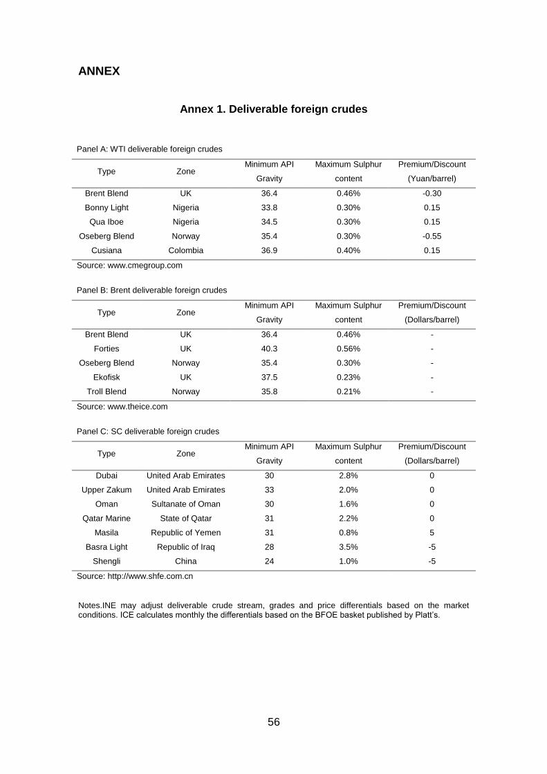
ANNEX

Annex 1. Deliverable foreign crudes

Panel A: WTI deliverable foreign crudes

Type Zone Minimum API

Gravity

Maximum Sulphur

content

Premium/Discount

(Yuan/barrel)

Brent Blend UK 36.4 0.46% -0.30

Bonny Light Nigeria 33.8 0.30% 0.15

Qua Iboe Nigeria 34.5 0.30% 0.15

Oseberg Blend Norway 35.4 0.30% -0.55

Cusiana Colombia 36.9 0.40% 0.15

Source: www.cmegroup.com

Panel B: Brent deliverable foreign crudes


Gravity

Maximum Sulphur

content

Premium/Discount

(Dollars/barrel)

Brent Blend UK 36.4 0.46% -

Forties UK 40.3 0.56% -

Oseberg Blend Norway 35.4 0.30% -

Ekofisk UK 37.5 0.23% -

Troll Blend Norway 35.8 0.21% -

Source: www.theice.com

Panel C: SC deliverable foreign crudes


Gravity

Maximum Sulphur

content

Premium/Discount

(Dollars/barrel)

Dubai United Arab Emirates 30 2.8% 0

Upper Zakum United Arab Emirates 33 2.0% 0

Oman Sultanate of Oman 30 1.6% 0

Qatar Marine State of Qatar 31 2.2% 0

Masila Republic of Yemen 31 0.8% 5

Basra Light Republic of Iraq 28 3.5% -5

Shengli China 24 1.0% -5

Source: http://www.shfe.com.cn

Notes.INE may adjust deliverable crude stream, grades and price differentials based on the market conditions. ICE calculates monthly the differentials based on the BFOE basket published by Platt’s.

http://www.cmegroup.com/

IS THE LEADERSHIP OF THE BRENT-WTI OIL FUTURES MARKET ...

Documents

Transcript of IS THE LEADERSHIP OF THE BRENT-WTI OIL FUTURES MARKET ...