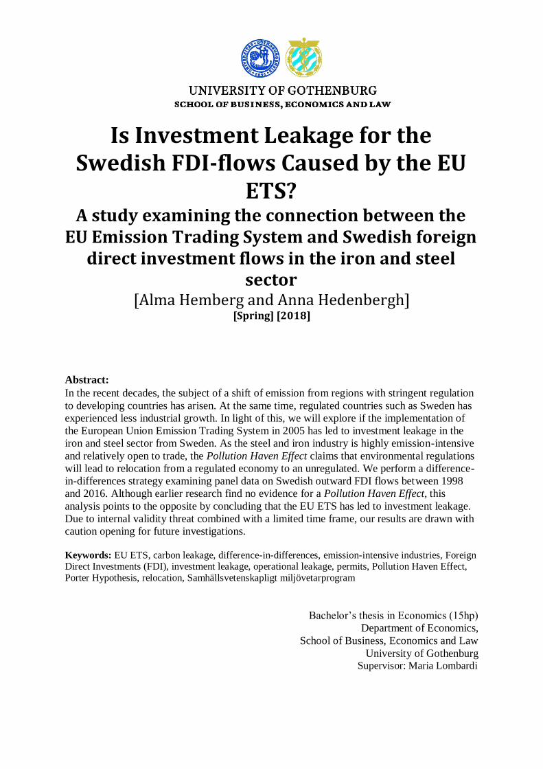
Is Investment Leakage for the Swedish FDI-flows Caused by the EU

ETS?

A study examining the connection between the EU Emission Trading System and Swedish foreign

direct investment flows in the iron and steel sector

[Alma Hemberg and Anna Hedenbergh] [Spring] [2018]

Abstract: In the recent decades, the subject of a shift of emission from regions with stringent regulation

to developing countries has arisen. At the same time, regulated countries such as Sweden has

experienced less industrial growth. In light of this, we will explore if the implementation of

the European Union Emission Trading System in 2005 has led to investment leakage in the

iron and steel sector from Sweden. As the steel and iron industry is highly emission-intensive

and relatively open to trade, the Pollution Haven Effect claims that environmental regulations

will lead to relocation from a regulated economy to an unregulated. We perform a difference-

in-differences strategy examining panel data on Swedish outward FDI flows between 1998

and 2016. Although earlier research find no evidence for a Pollution Haven Effect, this

analysis points to the opposite by concluding that the EU ETS has led to investment leakage.

Due to internal validity threat combined with a limited time frame, our results are drawn with

caution opening for future investigations. Keywords: EU ETS, carbon leakage, difference-in-differences, emission-intensive industries, Foreign Direct Investments (FDI), investment leakage, operational leakage, permits, Pollution Haven Effect, Porter Hypothesis, relocation, Samhällsvetenskapligt miljövetarprogram

Bachelor’s thesis in Economics (15hp)

Department of Economics,

School of Business, Economics and Law University of Gothenburg

Supervisor: Maria Lombardi

Acknowledgements: We are truly grateful for the statistics about Sweden´s FDI flows

received from Statistical Centralbyrån´s (SCB´s) Rickard Rens and the advices and guidance

from Maria Lombardi.

2

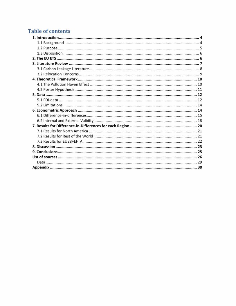
Table of contents

1. Introduction .............................................................................................................................. 4 1.1 Background ......................................................................................................................... 4 1.2 Purpose ............................................................................................................................... 5 1.3 Disposition .......................................................................................................................... 6

2. The EU ETS ................................................................................................................................ 6 3. Literature Review ..................................................................................................................... 7

3.1 Carbon Leakage Literature ................................................................................................... 8 3.2 Relocation Concerns ............................................................................................................ 9

4. Theoretical Framework ........................................................................................................... 10 4.1 The Pollution Haven Effect ................................................................................................ 10 4.2 Porter Hypothesis .............................................................................................................. 11

5. Data ........................................................................................................................................ 12 5.1 FDI-data ............................................................................................................................ 12 5.2 Limitations ........................................................................................................................ 14

6. Econometric Approach ........................................................................................................... 14 6.1 Difference-in-differences ................................................................................................... 15 6.2 Internal and External Validity............................................................................................. 18

7. Results for Difference-in-Differences for each Region ............................................................ 20 7.1 Results for North America ................................................................................................. 21 7.2 Results for Rest of the World ............................................................................................. 21 7.3 Results for EU28+EFTA ...................................................................................................... 22

8. Discussion ............................................................................................................................... 23 9. Conclusions ............................................................................................................................. 25 List of sources ............................................................................................................................. 26

Data ........................................................................................................................................ 29 Appendix .................................................................................................................................... 30

3

1. Introduction

1.1 Background Conventional wisdom in energy-intensive industries is that stricter climate policy weakens the

capability of performing in a competitive way because of large emission abatement costs and

asymmetric climate policies around the world (Zechter et al., 2017). Although different climate

policies are emerging globally, the first and largest regional carbon pricing system currently

implemented is the European Union Emissions Trading System (EU ETS). It is targeting energy

intensive industries with the aim of decreasing greenhouse gases (GHG) caused by the biggest

emitters among the EU28 plus Liechtenstein, Norway and Iceland (i.e. EFTA). The key

component to accomplish this is allocating a fixed number of tradable GHG allowances to the

polluters, and leaving the firms to buy and sell these allowances between one another.

Putting a price on carbon increases the threat of carbon leakage. Reinaud (2008) defines carbon

leakage “as the ratio of emissions increase from a specific sector outside the country (as a result

of a policy affecting that sector in the country) over the emission reductions in the sector (again,

as a result of the environmental policy)” (p.3). This leakage in emissions mainly takes place

through two channels: operational and investment leakage.

One concern of implementing environmental policy is that within a particular sector, the

constrained region faces certain costs whereas others, non-constrained regions, do not. This

creates a comparative disadvantage for the regulated economy to the benefit of non-constrained

regions. The additional costs may lead to operational leakage in the short-term, which means a

shift of market shares from the constrained region to foreign competitors that are not covered by

the regulations (Reinaud, 2008). In the long-run, the threat of industries relocating to countries

with laxer environmental regulations (investment leakage) is emerging. The overall consequence

would be an augmentation in GHG emissions globally, which is at the same time affecting the

international environment as well as the efficiency of climate policy.

Particularly sensitive sectors to these emission abatement costs are the ones that are highly CO2-

intensive and internationally open to trade, such as the iron and steel sector. The Alliance of

Energy Intensive Industries amongst others debates that the implementation of the

4

EU ETS is a contributing factor to European industries loss in competitiveness (European

Commission, n.d.a).

The purpose of this paper is to study investment leakage for the Swedish iron and steel industry.

The reason behind this is that this sector stands alone for 36 percent of total emissions in

Sweden, making it the largest emitting industry and undeniably a target for the EU ETS. Since

Sweden in the recent decades has experienced a diminishing industrial growth and at the same

time has increased outward foreign direct investment (FDI) flows, the worry of these flows

causing emissions in developing countries has arisen (SCB, n.d.; SCB, 2017). The total amount

of emissions on a Swedish national level has also decreased after 1990 (Naturvårdsverket, 2017),

which could advocate in favour for that emissions have moved outside the country.

Due to trade openness together with uneven climate policies, regulated nations may migrate their

production of energy-intensive goods to countries with more favorable climate policies. This is

known as the Pollution Haven Effect (Copeland & Taylor, 2004). To our knowledge, only a few

rigorous ex post studies has been made tackling investment leakage as a result of the EU ETS

(Koch & Houdou, 2016). Therefore this paper, as is the first of its kind using Swedish data, will

be exploring if the concern of relocation is valid with regards to the EU ETS. To further analyse

this issue, we will use FDI data provided by Statistiska Centralbyrån (SCB) on outward FDI

flows of Swedish firms.

1.2 Purpose This paper studies the potential consequences of the EU ETS in the iron and steel sector. More

precisely, we observe outbound FDI flows from Sweden possibly resulting from the regulation

(i.e. the long-run perspective, investment leakage). We focus on horizontal FDI, when a firm

invests in the same sector as the one they operate in their so-called home country (Feenstra &

Taylor, 2017, p. 23).

The reason to disregard operational leakage, the short-run perspective, is that Swedish steel

industry is highly niched and therefore in general not threatened to the same degree by

operational leakage as other countries producing conventional steel (Atallah, 2018, March 1st).

With this in mind, and the largest emission trading scheme being persistent and Sweden

5

being a target of it, we aim to examine whether the implementation of the EU ETS may have

induced investment leakage or not.

This potential outcome has its foundations in the Pollution Haven Effect as mentioned above. To

examine this belief, we apply a difference-in-difference (DID) strategy. Through a DID, we will

be able to compare the outcomes before and after the implementation of the EU ETS for a sector

affected by the policy change (in this case, the iron and steel sector) to an unaffected. Our

theoretical prediction is that outward FDI flows have increased in countries with less stringent

regulation since the implementation of the EU ETS. We have for that reason divided our

statistics into different regions and will then compare our findings for each region.

1.3 Disposition This paper is organized as follows. In section 2, we give a deeper background about the EU ETS.

Section 3 illustrates an overview of earlier research. After this, the relevant theoretical

frameworks are discussed in section 4. Then section 5 will describing the data and the limitations

concerning this. From there, in section 6, the econometric model will be both presented and

debated. Subsequently, our formed DID-model is tested in section 7 and results are portrayed.

Section 8 elaborates on our findings together with illustrating the current circumstances in the

iron and steel sector as well as what future research should focus on. Succeeding this, section 9

concludes this paper with emphasize on our discoveries. At last follows the references and

appendix.

2. The EU ETS

The EU ETS was launched in 2005 as a policy instrument aiming to reduce GHG emissions by at

least 40 percent in 2030 in comparison to historical output in 1990 (European Commission,

n.d.b). Operating in 31 countries in total, the mandatory emission trading scheme targets

approximately 11,000 energy-intensive installations as it covers about 45 percent of total GHG

emissions in the EU. The policy is based on the cap and trade principle where a cap is set

including a total amount of GHG emissions allowed (permits) by the companies covered by the

scheme. It is then up to the companies within the cap to trade permits between one another (if

they wish to do so), which makes this a market based instrument. The cap is then reduced each

year by a certain amount to continuously decrease

6

the environmental impact. Each permit gives the right to emit one ton of carbon dioxide, and the

total amount of permits is reduced throughout the years.

The system is divided into four phases. The first phase started with the implementation as a

“learning by doing” process between 2005 to 2007, where a generous cap of free allowances

was set based on estimated needs for targeted installations. The following trading period, phase

II, spanned the period from 2008 to 2012 corresponding with the Kyoto Protocol commitment.

Although a reduction of emission allowances by 6.5 percent was set in phase II, the economic

downturn in 2009 led to a surplus of allowances and the cap on permits remained large. Phase III

is the current phase covering the period from 2013 to 2020. Since 2013, the cap is reduced every

year, entailing a 21 percent reduction of GHG emissions compared to output in 2005. To achieve

the final goal of a 40 percent reduction by 2030, the phase IV (2021 to 2030) needs to be further

revised. With respect to emissions in 2005, the installations covered by the system need to

reduce their GHG emissions by a total of 43 percent by the end of phase IV. This will be

undertaken by yearly reducing the cap by 2.2 percent from 2021 onwards.

By being the first to put a price on carbon, the EU ETS is facing a challenge of lower emissions

in regulated areas while the opposite in the so called third countries (i.e. carbon leakage). In

order to address this concern, the EC has developed the free allocation of permits. This has since

the implementation been the dominant principle of allocation, since it is advocated to help

preventing the risk of carbon leakage. The alternative way of allocation is auctioning of permits,

which is progressively taking place in the majority of the sectors covered by the scheme. As free

allocation is the main argument to prevent carbon leakage, the EC has acted very precautionary

in carbon-intensive industries concerning auctioning. However, since the share of auctioning is

expected to rise significantly in manufacturing industry in the future, associations such as Energy

Intensive Industries (n.d.) has been lobbying against the opening up of auctions.

3. Literature Review The existing evidence about the amount of spillover effects that can be expected due to

environmental regulations is not conclusive. Common knowledge advocates that environmental

regulations weaken the capability of firms to act in a competitive way, whereas

7

many empirical studies do not find support for this. This section will discuss earlier research

assessing carbon leakage together with different aspects and consequences of relocation.

3.1 Carbon Leakage Literature Branger et al. (2016) study the carbon leakage effect from the EU ETS, and show that it is non-

existent. The authors tested this belief for the cement and steel industry, as these sectors are

energy-intensive and likely to be vulnerable for climate policy. Even though these sectors are

vulnerable, no evidence for operational leakage could be proven. By using European emission

allowances (EUA) prices as their main regression variable, Branger et al. conclude that prices on

EUA has little to no impact on the competitiveness of a firm. However, the authors could not

conclude that free allocation of allowances should be scrapped, as they disregard the production

capacity perspective (i.e. leakage through the investment channel). They referred to the question

of investment leakage as an open question, as this particular research area is relatively

undiscovered.

Koch and Houdou (2016) focus on the issue of production capacity, by studying FDI data on

German manufacturing firms. This was applied on a DID analysis with one country being an EU

ETS member while the other country is not. The authors conclude that only a small share of the

studied firms experienced industrial relocation to a non-EU ETS member since the

implementation of the scheme. However, their results cannot be solely attributed to the EU ETS

implementation, as the concerned firms did not operate in an emission intensive nor an energy-

intensive industry. They further claim that the reason to this could be that many EU ETS firms

that are emission-intensive often also are capital-intensive with high fixed plant costs, which

creates relatively high relocation costs.

In contrast to studies mentioned above, Aichele and Felbermayr (2012) assessed carbon leakage

as a result of the Kyoto protocol and found empirical evidence for this. By using a DID

approach, they investigated the impact of the Kyoto protocol comparing CO2 emissions with

CO2 net imports and carbon footprint in countries committed to the agreement. The authors

conclude that the Kyoto protocol has led to domestic emission savings by about 7 percent but

without changing the carbon footprint. This ex post study showed a 14 percent increase in net

import of carbon dioxide, and thereby indicating (although not explicitly formulated) a carbon

leakage estimation of about 100% since the implementation of the protocol. In similarity with the

EU ETS, the Kyoto protocol exempts emerging and

8

developing countries, which raises the question of the pollution haven effect as a consequence of

the EU ETS.

Wu (2013) concludes that that Pollution Haven Effect is a valid concern for the European Union

as the stringency of the EU ETS is believed to be the cause behind emissions shift to regions

with laxer regulation. To study this connection, Wu employs a difference-in-differences strategy

by analyzing panel bilateral trade flows data. This data is then divided into two groups, the trade

flows outside and inside the European Union. Her findings for the steel and iron industry, in

contrast to her identified Pollution Haven Effect, demonstrates that the EU ETS has led to higher

export flows while the opposite holds for imports. Lastly, Wu opens up for future research to

investigate this relocation matter by looking at regarding domestic production and foreign direct

investment.

3.2 Relocation Concerns Martin et al. (2014) study the vulnerability to carbon pricing in firms regulated by the EU ETS.

They identify two main relocation concerns from climate policy: relocation creates costs in terms

of job losses to unregulated countries and weakens the effectiveness of the policy (since GHG is

a global public bad). The authors provide a qualitative study interviewing 761 manufacturing

firms in 6 European countries to examine firms’ propensity to downsize or relocate in response

to climate change policy. They conclude that an average firm would neither relocate outside the

ETS-borders nor fully shut down the company as a result of the EU ETS. There exists however a

substantial variation in the reported vulnerability between sectors, and the iron and steel industry

is according to the study among the most vulnerable ones.

Oikonomou et al. (2006) also claim that environmental regulations are unlikely to have a

substantial impact on relocation. They point out that when considering relocation, pollution

abatement costs are generally lower than other costs such as tariffs, exchange rate volatility,

transport costs and availability of qualified labour. Thus, pollution abatement costs are declared

to be unlikely to impact relocation. However, Ederington et al. (2005) argue that there in fact are

industries where those costs are relatively notable. In those cases, the concerned industries turned

out to be very capital intensive and this diminished their incentives to relocate. Yet again, other

costs exceeded the actual pollution abatement costs

9

and hence the study by Ederlington et al. (2005) corresponds to the conclusions reached by

Oikonomou et al. (2006).

Concerning the warnings about the relocation of industries outside the EU, Koch and Houdou

(2016) convey that they are rather used as motives by firms to lobby for higher levels of permits

than an actual threat. BusinessEurope (2016) sympathizes with this idea as they describe it as an

overstatement, by pointing out that location is the last determining factor in carrying out an

investment decision. They thereby express that the concern about more stringent environmental

regulation is not likely to be the deciding factor for relocation in such a scheme as the EU ETS.

However, relocation is still a highly debated subject in the research surrounding leakage for

environmental policies as the diverse results founded by Koch and Houdou (2016), Branger et al.

(2016) and Wu (2013) shows. This diverge conclusions from studies motivates why this belief

should be explored in greater detail which we examine in connection to investment leakage.

4. Theoretical Framework

4.1 The Pollution Haven Effect The Pollution Haven Hypothesis emerged with the purpose of highlighting the potential

environmental impacts caused by the liberalization of international trade (Brunnermeier and

Levinson, 2004). The hypothesis states that a reduction of trade barriers will result in emission-

intensive industries shifting their production from the regulated part to the unregulated part of the

world. Regions that experience these changes in FDI inflows are known as pollution havens. An

example of this could be that more stringent regulation inside the EU cause higher FDI outflows

to developing regions such as Asia.

The Pollution Haven Hypothesis has its theoretical foundations in the Heckscher-Ohlin Model

(Hille, 2015). In this context, the comparative disadvantage for carbon-constrained industries is

the additional pollution abatement costs they face in relation to their foreign competitors. This

could either result in losses of market share (operational leakage) or, at longer term, lead to

relocation to pollution havens. However, the actual magnitude of pollution abatement costs is, as

mentioned in the previous section, widely discussed.

10

According to Copeland and Taylor (2004), a distinction between the Pollution Haven Hypothesis

and the Pollution Haven Effect should be made. They refer to the ‘Hypothesis’ as the effects of

trade openness, whereas the ‘Effect’ refers to the consequences of a stringency in pollution

regulation. In this context, the latter would be the central concept of this paper.

Although the Pollution Haven Hypothesis often appear as an argument against environmental

regulations, the existence and strength of it have yet been difficult to prove empirically. A

common argument of its existence is the absence of ambitious climate policies in regions other

than the EU, and that the only solution for effective climate policy would be a globally

coordinated climate agreement (European Commission, n.d.a). Until such a binding international

agreement has taken place, the concern of pollution havens should still be considered as

environmental regulations are emerging.

The theoretical prediction for pollution haven is that we will find positive amounts in billion

SEK for North America and Rest of the World (ROW). We would expect the opposite to hold for

EU28+EFTA as the outward FDI flows to this region is expected to decrease due to the EU ETS.

This would then be in line with the ‘Effect’, which advocates higher FDI flows to North America

as well as ROW while the contrary would hold for EU28+EFTA.

4.2 Porter Hypothesis Historically, the view of stricter environmental regulation has been rather negative. The

traditional outlook is that decreasing an externality such as air pollution, which a strict

environmental regulation does, limits the regulated firms’ options and thereby reduce their profit

(Ambec et al., 2011). Porter (1991) contributed to this with a new angle by stating that “Strict

environmental regulations do not inevitably hinder competitive advantage against rivals; indeed,

they often enhance it” (p. 168). This is commonly referred to as the Porter hypothesis (PH)

(Brännlund, 2007), which says that environmental regulation will lead to firms investing in

research and development (R&D). Firms then either increase their productivity which in turn

leads to lower costs or commit to product development that gives of a higher product value. Both

of these options according to Porter results in improvement in competitive advantage. By

declaring this idea, Porter also brings new light to the earlier less adverse perspective of negative

externalities and gives insights on the positive effects a stricter regulation may result in.

11

Together with his co-author van der Linde, Porter claims that stricter regulation also results in

more innovation (Porter & van der Linde, 1995). These new clean innovations may decrease the

carbon footprint, thus improving the environment. This would imply that the innovation effects,

that would be created by this connection between innovation and regulation, would lead to the

regulated parties experiencing less additional costs (Ambec et al., 2011). The reason behind this

is that regulation generates pressure, which in turn lays the foundations for motivations to

innovation and progress. Although the theory of Porters and van der Linde has been thoroughly

discussed, it is today viewed as a theory to explain the connections behind stricter regulation and

more innovation. This provides support for more stringent environmental regulation, which is

very needed with the rising trend of environmental policies emerging (Ambec et al. 2011).

Research such as Martin and al. (2016) suggest the aspect of clean technology should be further

explored by looking into if clean innovation creates repercussions for macroeconomic growth by

crowding out of dirty innovations. According to our research, we are yet to find a strong link

between EU ETS and the Porter Hypothesis and thereby these ideas will be further debated in the

context of this paper.

With regards to the Porter Hypothesis, the previous prediction about investment leakage might

not hold. If Swedish firms find a way to become more productive by investing in innovation as a

result of the policy, then they might not relocate and would hence diminish FDI outflows.

5. Data The purpose of this paper is to study the impact of EU ETS on investment leakage, by using

foreign direct investment (FDI) as a measure of leakages. A FDI is taking place when an

investment is made cross-border by an investor in one country with purpose to establish a

durable interest in another country. The ‘durable interest’ is attained when the investor owns at

least 10 percent of the enterprise invested in (OECD, 2008). As earlier mentioned, outward FDI

flows (referring to energy-intensive investments) could amount to negative environmental

impacts in other countries which is the objective to examine in this paper.

5.1 FDI-data

To put this in an econometric perspective, we use foreign direct investment (FDI) outflows

(assets per sector) as the dependent variable in our regression. We rely on yearly measured data

from Statistiska Centralbyråns (SCB) statistical database, measured in billion SEK, that

12

spans the period from 1998 to 2016. As the EU ETS was implemented in 2005, the ex ante

period is from 1998 to 2004 and ex post is 2005 to 2016.

The data is divided into three different country groups: EU28+EFTA, North America and the rest

of the world (ROW). This leads to three different DID analyses. Considering there are already a

few ETS implemented in the world (although not in the same magnitude as the EU ETS), five

countries are excluded from ROW (Switzerland, Kazakhstan, South Korea, Australia and New

Zealand) (Carbon Market Data, n.d.). Even though there are cap-and-trade schemes implemented

in both the United States (US) and Canada, we consider that testing for North America is still of

high relevance. This is partly because the steel export market to the US is very vital for Sweden,

and partly because the magnitude of the cap-and-trade systems compared to the EU ETS is

relatively small (Atallah, 2018, March 1st; European Commission, n.d.a). The one closest to the

size of the EU ETS, California’s cap-and-trade program, was first launched eight years after the

EU ETS and is mainly targeting the transportation sector (ICAP, 2018).

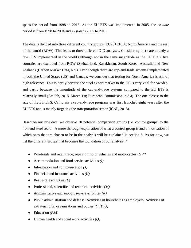
Based on our raw data, we observe 10 potential comparison groups (i.e. control groups) to the

iron and steel sector. A more thorough explanation of what a control group is and a motivation of

which ones that are chosen to be in the analysis will be explained in section 6. As for now, we

list the different groups that becomes the foundation of our analysis. *

● Wholesale and retail trade; repair of motor vehicles and motorcycles (G)**

● Accommodation and food service activities (I)

● Information and communication (J)

● Financial and insurance activities (K)

● Real estate activities (L)

● Professional, scientific and technical activities (M)

● Administrative and support service activities (N)

● Public administration and defense; Activities of households as employers; Activities of

extraterritorial organizations and bodies (O_T_U)

● Education (P85)

● Human health and social work activities (Q)

13

What separates these sectors from the iron and steel industry is that they are not emission nor

energy intensive and unregulated by the EU ETS, which makes them valid comparison groups

for the analysis. As the FDI data is measured in billion SEK, the analysis will be run in levels.

*For full data material, see Appendix. ** The letter in the parenthesis is the one corresponding

to a specific sector according to the Swedish classification system SNI (SCB, 2007)

5.2 Limitations To conduct a richer analysis, it would be preferable that our data were disaggregated into finer

regions. The threat of possessing aggregated data is that it might lead to overestimation of the

Pollution Haven Effect. This because if in the ROW there are countries which are not pollution

havens, the expected result would be no effect. Unfortunately, a more country-specific data

requested from SCB led to a large number of data points being unavailable because of secrecy.

Choosing the more country-specific data would lead to ignoring numbers in countries that are

large steel producers, such as China, India, Turkey and Russia and would thereby weaken the

reliability. With a more aggregated data, which we will run our analysis on, we were able to

include these important countries in ROW. Nevertheless, data on Swedish FDI outflow to North

America was unavailable in 2014 which we solved through interpolation.

Another important aspect is that the assets abroad are presented in the Swedish companies sector

affiliations, as the sector of the foreign asset is not specified. This means that if for example a

Swedish steel company owns foreign companies within other sectors, these assets will be shown

as steel industry. The assumption is further supported by the presence of horizontal FDI flows for

the steel sector, in form of the Swedish SSAB investment in the American steel firm IPSCO after

the implementation of EU ETS (Sunnesson, 2008, May 20th; SSAB, 2007, May 3rd). However,

an overall trend of horizontal FDI flows into the same sector can not be assumed. In light of this,

if there are spillovers in other sectors, that is something we will be forced to ignore in this

analysis.

6. Econometric Approach Two common methods for quasi-experimentally testing the impact of a policy changes are

simple before-after difference and difference-in-differences strategy (Mitrut, 2018a). The

14

before-after strategy is generally practiced by comparing the relevant outcome variables before

and after the policy is implemented, to discover any possible connections that can be derived as a

result of the policy itself (Mitrut, 2018b). However, a drawback of this strategy is that it

disregards of other factors that are trending between the studied years that may account for the

change in the outcome of interest.

For the purpose of this paper, this neglect is truly problematic as the influence of other

macroeconomic factors that change over time most likely will be high. In order to overcome this

issue, we adopt a difference-in-differences (DID) strategy since the method allows to control for

different factors apart from the policy change that might otherwise lead to biased estimates

(Mitrut, 2018a).

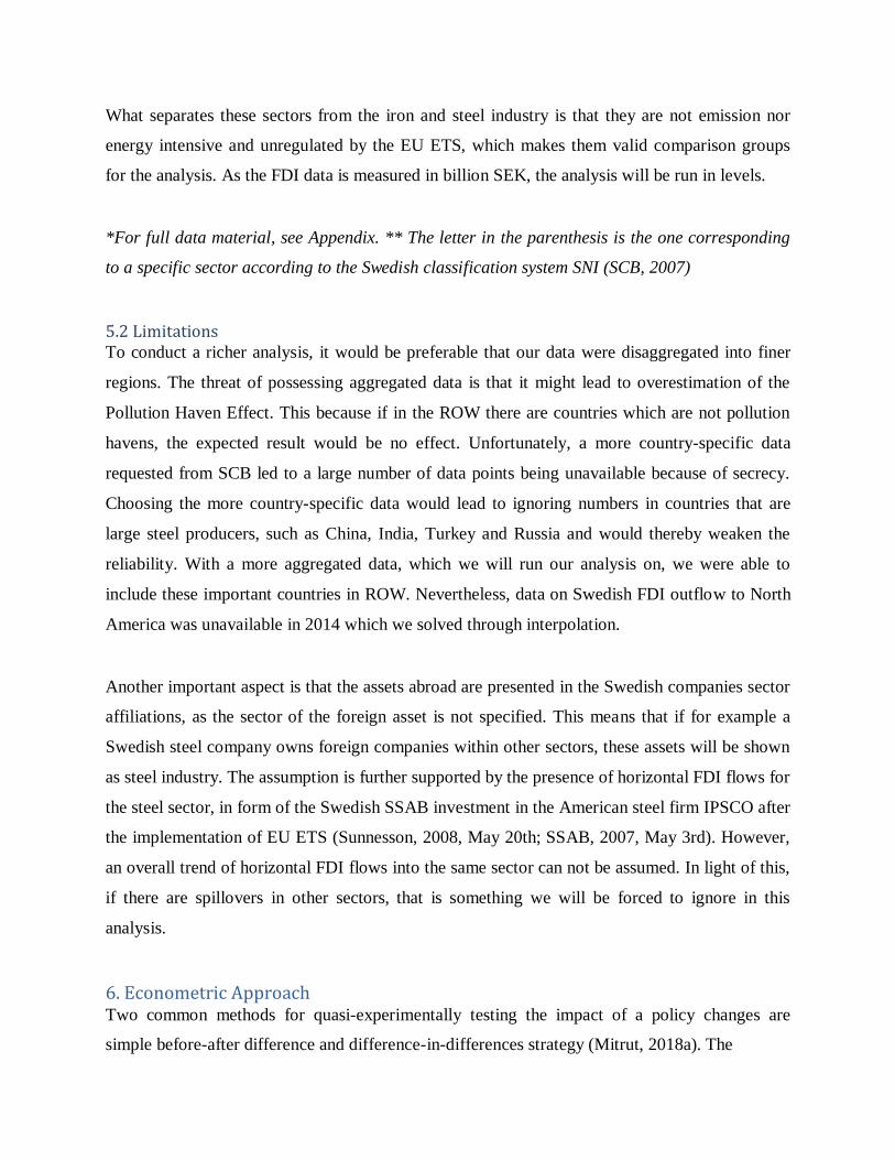
6.1 Difference-in-differences Figure 1 shows annual Swedish outward FDI flows to North America in ‘Manufacture of iron

and steel products’ (blue line) and ‘Professional, scientific and technical activities’ (orange line).

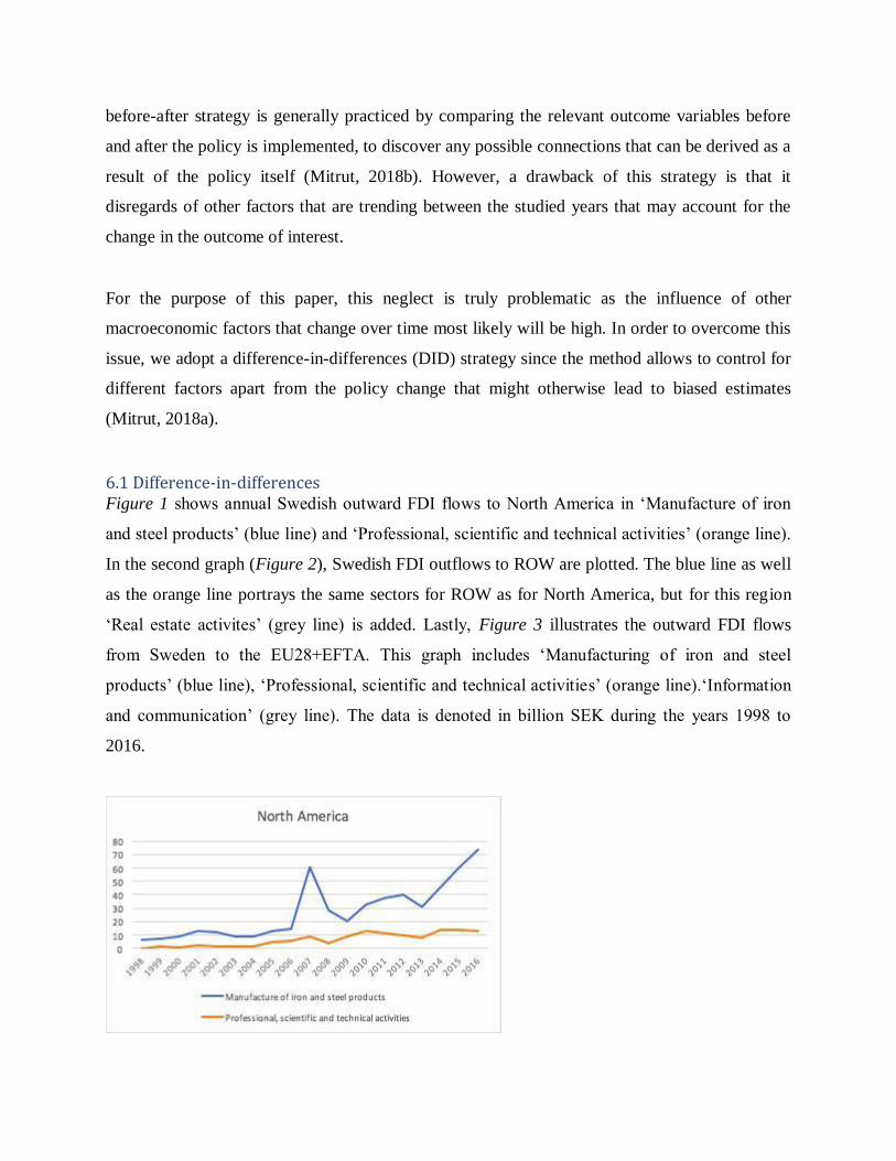
In the second graph (Figure 2), Swedish FDI outflows to ROW are plotted. The blue line as well

as the orange line portrays the same sectors for ROW as for North America, but for this region

‘Real estate activites’ (grey line) is added. Lastly, Figure 3 illustrates the outward FDI flows

from Sweden to the EU28+EFTA. This graph includes ‘Manufacturing of iron and steel

products’ (blue line), ‘Professional, scientific and technical activities’ (orange line).‘Information

and communication’ (grey line). The data is denoted in billion SEK during the years 1998 to

2016.

Figure 1. Swedish FDI outflows to North America for the chosen sectors

15

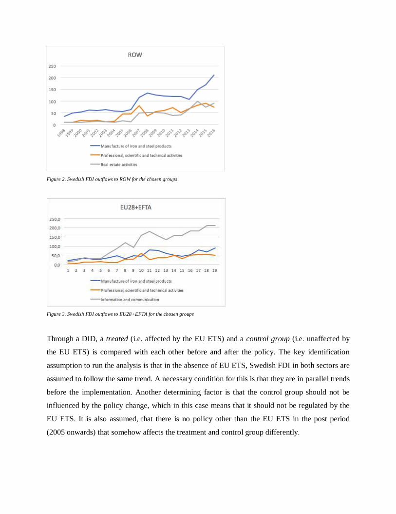
Figure 2. Swedish FDI outflows to ROW for the chosen groups

Figure 3. Swedish FDI outflows to EU28+EFTA for the chosen groups

Through a DID, a treated (i.e. affected by the EU ETS) and a control group (i.e. unaffected by

the EU ETS) is compared with each other before and after the policy. The key identification

assumption to run the analysis is that in the absence of EU ETS, Swedish FDI in both sectors are

assumed to follow the same trend. A necessary condition for this is that they are in parallel trends

before the implementation. Another determining factor is that the control group should not be

influenced by the policy change, which in this case means that it should not be regulated by the

EU ETS. It is also assumed, that there is no policy other than the EU ETS in the post period

(2005 onwards) that somehow affects the treatment and control group differently.

As shown in Figure 1, both treatment and control group follow a similar trend for FDI outflows

to North America. The same holds for the three groups in ROW (Figure 2). This

16

makes the chosen groups valid alternatives as control groups for a DID analysis. In contrast to

this, the EU28+EFTA (Figure 3) is lacking similar trends before the EU ETS was enforced in

2005 and thus the causal interpretation for this region diminishes. However, we consider it useful

include this region in the analysis as it provides enriching information for the discussion and

future research.

The reason why the control groups differ between the regions is because different sectors were in

parallel trends with the iron and steel sector in each region group. In North America, there was

only one group comparable to the iron and steel sector in the pre-period based on key assumption

and hence this region provides only one control group. In total, there are three control groups

chosen from the 10 potential comparison groups earlier listed. To illustrate that these sectors are

not regulated by the EU ETS, a more detailed explanation of each control group is described

below.

● ‘Professional, scientific and technical activities’ (M) (SCB, 2007).

This consist of legal affairs in form of activities in lawyer firms, legal agencies and

agencies focusing on patent issues. Besides that, this control group partly includes

affairs concerning accounting and tax advice as well other economic consulting affairs

is. Additionally, it contains of consultancy services and what is labelled as architecture

and technical consultancy. The statistics for FDI flows for the scientific research and

development together with advertising and market surveys is also derived from this

group.

● ‘Real estate activities’(L)

Incorporates trade with owned real estate, rent as well as management of owned and

leased these types of properties. Except these, are also real estate agencies and

management of real estate by assignment part of this category.

● ‘Information and communication’ (J)

Contains publisher affairs such as the publications of books and newspapers. Another

part of this is releases of films, video- and TV-programs that concerns the whole

production process. Furthermore, it involves telecommunications, computer

programming together with data consultancy and information services as news

services and data processing.

17

For each region group, we run the following difference-in-differences regression for 1998 to

2016: FDIi,t = β0 + β1Steeli + β2Postt +β3Steeli∗Postt+ δt + Ui,t

FDIi,t = monetary amount in outward FDI in year t in sector i (outcome variable)

Steel = 1 if the industry is steel, and 0 if not (treatment variable)

Post = 1 in the period in which the EU ETS is in place (from 2005 onwards)

δt = year fixed effects (capture year-specific shocks affecting FDI flows in both sectors)

Ui,t = the error term, which captures unobservable determinants of FDI flows in a year t in

industry i.

Our main interest in this regression is the interaction term, i.e. the causal effect of interest

(Dzemski, 2018). It estimates the difference between the average change, in billion SEK, in FDI

in the control group and the average change in the treatment group from 1998 to 2016. This

results in an interpretation whether the EU ETS had an impact on Swedish FDI outflows or not.

6.2 Internal and External Validity

As in any quasi-experimental study, validity is divided into two separate segments: internal and

external validity (Meyer, 1995). Both of these will be discussed and reviewed with regards to the

paper’s purpose of analyzing investment leakage for Swedish FDI flows.

To analyze our panel data, we have opted to apply fixed effects (FE) (Gujarati and Porter, 2009,

p. 599-602). This is an advantage for the analysis that leads to less biased estimates, as it covers

for yearly global shocks that may affect both groups simultaneously.

In this case, the main threat to internal validity concerns factors in the ex post period that may

affect the two groups differently. For example, the financial crisis in 2008 affected the real estate

pricing which may have affected the FDI in ‘Real estate activities’ to ROW. However, Figure 2

does not show any larger downward fluctuation around this year. Another example of internal

validity threat could be changes in relative prices in the steel sector compared to the control

group, or lower raw material prices within the steel sector outside the EU that

18

attracts investments in this particular sector. These concerns are not taken into consideration in

this analysis, as our model would conclude all increase in FDI flows as a result of the EU ETS. If

there are other factors determining the choice of relocation in this period (which most likely is

the case), our estimates could be biased. We acknowledge these limitations, and thus interpret

our results with caution.

From a validity standpoint, it is important to also cover the external validity. Meyer (1995)

discuss how the effect of the treatment may fluctuate over time periods. For our model, this can

be problematic as we are looking at three different phases and time periods for the EU ETS. We

are aware of the looser cap in the beginning of the scheme (phase I) as well as the excessive cap

in connection with the financial crisis (phase II).

19

7. Results for Difference-in-Differences for each Region

Table 1. An overview of every performed regression for each

region

North America Rest of World

Prof., Sc. & Tech. Real est. Prof., Sc. & Tech. Info. & Com.

Type of (1) (2)

(1) (2) (1) (2)

(1)

reg.

Steel x 20.489*** 20.489*** 27.924* 27.924** 20.854 20.854* -93.717***

Post (5.733) (5.003) (14.821) (7.615) (13.716) (10.573) (15.182)

Steel 7.786*** 7.786*** 43.543*** 43.543*** 40.571*** 40.571*** -8.400

(0.955) (0.718)

(3.756) (3.477) (3.977) (3.021)

(9.783)

Post 8.120*** -

42.191*** -

49.261*** -

122.032***

(1.060)

(7.682) (5.240)

(13.935)

Obs. 38 38 38 38 38 38 38

R2

0.6585 0.8693 0.7062 0.9651 0.7235 0.9177 0.8395

Year FE x x x

Notes: These regressions were performed by using panel data from year 1998 to 2016. The table present the regressions for each region.

Every variable, except R2, is round off to three decimals. The

specification in regression (2) includes year fixed effects. Robust standard errors is found inside the parentheses. Post is omitted for regression (2) because of collinearity and thereby these coefficients are not included in the table. Significance level are noted as follow 1(***), 5(**) and 10(*).

2

0

7.1 Results for North America For North America, our coefficient of interest in regression (1) is taking a value of 20.489 and is

significant at the 1 percent level. This means that after 2005, average annual FDI in the iron and

steel sector was 20.489 billion SEK higher than “Professional, scientific and technical activities”.

The Steel coefficient shows that before the regulation, Swedish annual FDI outflow was higher

in the iron and steel sector than in the control group. By analyzing the post coefficient, we

observe that both sectors have experienced increasing FDI flows from Sweden in the post period.

Regression in column (2) includes year fixed effects to control for year specific shocks affecting

both industries. In regression (2), we find that the coefficient of interest is the same as regression

(1) at 20.489, thereby the same interpretation applies here. The Steel coefficient is unchanged,

only more precisely estimated just as the coefficient of interest. These findings support that our

conclusions for regression (1) is correct. The R2 in regression (2) has also increased from 0.6585

to 0.8693 when controlling for fixed effects, which indicates that a big part of the explanation is

due to yearly variations. Therefore, we can conclude that investment leakage is present for North

America due to the EU ETS, as Steel x Post is positive and significant in both regressions.

7.2 Results for Rest of the World By performing regressions for ROW two control groups are applied: ‘Real estate activities’ and

‘Professional, scientific and technical activities’.

7.2.1 Real estate activities In regression (1), the coefficient of Steel x Post is 27.924 and is significant at the 10 percent

level. This stands for the growth in outward FDI flows from Sweden in the iron and steel

industry after 2005 in billion SEK in contrast to `Real estate activities´, which is deemed as a

result of the policy. The coefficient for Steel at 43.543 reveals that the iron and steel sector had

higher FDI flows than in the control group. It is evident when regarding the Post coefficient that,

for both sectors, Swedish FDI outflows are trending upwards from 2005 onwards.

For regression (2), when fixed effect for years are included, the Steel x Post is significant at the 5

percent level. The standard errors have decreased from 14.822 to 7.615, and explanatory

21

power (R2) has increased by about 32 percentage points. This again strengthens the controlling

for fixed effects as we through this discover that a lot of explanation of the model is due to

yearly variations. We also observe an unchanged, more precise estimation of the Steel

coefficient.

We observe more significant and more precisely estimated coefficients, which indicates that

investment leakage in the iron and steel sector has taken place in ROW due to the EU ETS.

7.2.2 Professional, scientific and technical activities As we can see in the first regression when comparing the iron and steel sector with ‘Professional,

scientific and technical activities’, the coefficient of interest is insignificant. The Steel and Post

coefficients are however showing significant values at the 1 percent level, and explanatory power

is high. We conclude that Swedish annual FDI outflow was 40.571 billion SEK higher in the iron

and steel sector in relation to the control one, and an upgoing trend is present from 2005

onwards.

From regression (2), an indication of investment leakage is spotted. The coefficient of interest,

showing a value of 20.854, is significant at the 10 percent level and Steel coefficient remains

unchanged and significant. Controlling for fixed effects yet again increases the explanatory

power and provides more precise estimates. Thereby the same conclusion as with ‘Real estate

activities’ is drawn here, which further strengthens the conclusion of investment leakage to North

America being present.

7.3 Results for EU28+EFTA In this case, we expect an inverse result in comparison with the other two. This is because we

now use data on Swedish FDI outflows inside the regulated area of the EU ETS (Sweden

excluded). After 2005, average annual FDI in treatment group is expected to be lower than in the

control one. Econometrically speaking, this implies that our coefficient of interest, Steel x Post,

should be negative. One important aspect is that the key assumption for this region cannot be

stated (see Figure 3) and hence the causal interpretation diminishes. Despite this, we include

these regressions as it provides information about the development of FDI flows within

EU28+EFTA.

22

As expected, Steel x Post is negative regardless of which is the control group. This coefficient

for ‘Professional, scientific and technical activities’ is however far from significant, contrasting

with the one for ‘Information and communication’ with high significance in both regressions.

One striking observation in ‘Information and communication’ is that the Steel coefficient shows

that the average FDI for the two sectors is not statistically different from zero in the pre-period,

whereas the interaction variable show a large statistically significant difference in the two

sectors.

As mentioned above, a conclusive conclusion about the impact of the EU ETS on FDI outflows

in the iron in steel sector is not possible for this region. If parallel trends assumption would hold,

the conclusion would vary depending on which is the control group. This indicates that any

conclusion about investment leakage should be drawn with caution, as the results are contrasting

each other and thereby we leave this open for future investigations.

8. Discussion The majority of our findings points to investment leakage in each region. This contradicts most

of what has been determined by earlier literature, where the prevailing conclusion is that

environmental regulations have a small to negligible impact on relocations (Oikonomou et al.,

2006). However, as investment leakage due to the EU ETS in particular is a relatively

undiscovered area it would be irrational to directly connect earlier research with this paper.

One can however elaborate on aspects that somehow could enrichen the analysis. Future research

could investigate investment leakage in other emission-intensive sectors than the iron and steel

secor. This would strengthen (or question) the conclusions drawn from this analysis. Inclusion of

more variables to the analysis is also to consider for future research, not least concerning the cost

aspect. As stated by Ederington et al. (2005), emission-intensive industries such as the iron and

steel sector face large relocation costs which should be taken into consideration when examining

investment leakage. A deeper analysis of the impact of other parameters such as for example

trade barriers and political as well as economic risk on relocation to developing countries could

also add significant value in this question (Oikonomou et al., 2006).

Approaching the Porter Hypothesis, the Swedish steel market has lately shown commitment in

environmentally friendly technology by investing in green steel (Löfvenberg, 2018,

23

February 5th). This is when steel is produced with less GHG emissions as the use of coal is

extracted from the production process. Three Swedish firms (LKAB, SSAB and Vattenfall) has

committed to the so called HYBRIT project, which is a production facility with the goal of

making green steel. The project strives to emit no GHG emissions in the steel production. Should

the pursuance become successful, the project may reduce CO2-emissions on a Swedish national

level by 10 percent (TT, 2018, January 21th). It might also in the long run prove to be a

profitable strategic investment decision for the firms, especially since the restrictions from the

EU ETS has become stricter for each phase and that this trend seems to continue. Besides this,

SSAB (2018, February 1st) argues that the HYBRIT project may be the crucial tool that is

needed for Sweden to fulfill its commitments according to the Paris Agreement. The existence of

this project may strengthen the claims made by Porter and van der Linde in the context of the EU

ETS. However, by our research we cannot spot any impacts of stricter environmental goal

resulting in innovation effects nor enhanced competitiveness level between firms. Besides,

according to the analysis conducted here, the dominating theory seems to be the Pollution Haven

Effect.

With further regards to the clean innovation aspect, Vestre (2018) mentions that SSAB offer the

most environmentally friendly steel on a global level. Their steel emits 26 percent less than its

Chinese counterparts. We will avoid discussing the market implications that this might have for

investment leakage as it lies outside the context of this paper. But, once again, that might point at

an innovation effect within the Swedish borders. This could be due to the stricter environmental

regulation in form of the EU ETS, which Porter and van der Linde argues for. As the innovation

effects or any connections to the Porter Hypothesis is at the present unclear, future research

could further explore this.

To summarize, future research should keep examining the connection between investment

leakage and Pollution Haven Effect with regards to the EU ETS. Except that, an interesting

approach would be the potential innovation effects resulting from the climate policy. In such

case we suggest a qualitative study focusing on questions around contributing factors to

innovation investments. We look forward to see how this research area will develop throughout

the years.

24

9. Conclusions Our findings through the DID analysis indicates a significant investment leakage within the iron

and steel sector to North America and ROW. We also find suggestive evidence of negative

spillovers in the steel sector in the case of EU28+EFTA, although the parallel trends assumption

does not hold in this case. As shown in Figure 3, and strengthened by the regression, we observe

a larger difference in average annual FDI flows in the post period for this region (outward FDI

within the iron and steel sector is significantly lower in the post period compared to ‘Information

and Communication’). However, due to the violation of the key identification assumption, we

cannot attribute all of this to the EU ETS.

In those cases when significant investment leakage was found, data at country-specific level

would be preferable. Especially in the case of ROW, as we have experienced hardships when

identifying the potential pollution havens arising from the policy. This means that we cannot

distinguish if the FDI has gone mainly to developing countries as for example Pakistan or to a

more developed country such as Taiwan.

However, we consider that these conclusions about a significant investment leakage should be

drawn with caution. One reason for this is that the results are not corresponding to the majority

of earlier empirical studies on carbon leakage and pollution haven literature. This inevitably

raises the question of the validity in our model. Referring to our main internal validity threat, the

reasons could be many. For example, price dumping of steel prices in China and Russia

happening simultaneously as the EU is recovering from the financial crisis in 2008 can be

considered as one of these concerns. This may not have affected the highly niched Swedish steel,

but could be a contributing factor to why FDI outflows in the iron and steel industry are not

trending in the same way as our chosen control group. It could also indicate that the relative

prices of producing steel outside the EU is decreasing and hence is attracting investments in

ROW and North America. One can speculate if these actions have affected the Swedish

investment decisions, but due to the lack of data and the limited time frame we leave this as an

open question for future research.

25

List of sources Aichele, R. & Felbermayr, G. (2012). Kyoto and the carbon footprint of nations. Journal of

Environmental Economics and Management, 63(3), 336-354. doi:10.1016/j.jeem.2011.10.005

Ambec, S., Cohen, M. A., Elgie, S., & Lanoie, P. (2011). The Porter Hypothesis at 20: Can

Environmental Regulation Enhance Innovation and Competitiveness? (RFF DP, No. 11-01).

Retrieved from Resources for the Future (RFF) website:

http://www.rff.org/files/sharepoint/WorkImages/Download/RFF-DP-11-01.pdf

Atallah, C. (2018, March 1st). Stålindustrin: “Det kommer att påverka”. SVT Nyheter. Retrieved 2018-04-29, from https://www.svt.se/nyheter/inrikes/stalindustrin-vi-drabbas-inte-

lika-hart-som-kina

Branger, F. & Quirion, P. (2014). Climate policy and the ‘carbon haven’ effect. WIREs Clim Change 2014, 5(1), 53-71. doi:10.1002/wcc.245

Branger, F., Chevallier, J. & Quirion, P. (2016). Carbon Leakage and Competitiveness of

Cement and Steel Industries under the EU ETS: Much Ado about Nothing. The Energy

Journal, 37(3), 109-135. doi:10.5547/01956574.37.3fbra

Brunnermeier, S. B. & Levinson, A. (2004). Explaining the Evidence on Environmental

Regulations and Industry Location. Journal of Environment & Development, 13(1), 6-41. doi:10.1177/1070496503256500

Brännlund, R. (2007). Miljöpolitik utan kostnader? (Elektronisk resurs): en kritisk granskning

av Porterhypotesen. Stockholm: Finansdepartementet.

BusinessEurope. (2016). BUSINESSEUROPE comments on the Commission’s EU ETS reform proposal. (Online). Available at:

https://www.businesseurope.eu/sites/buseur/files/media/position_papers/iaco/2016-02-

10_ets_reform.pdf

Carbon Market Data. (n.d.). World Carbon Market Database. Retrieved 2018-05-08, from

https://www.carbonmarketdata.com/en/products/world-ets-database/presentation

Copeland, B. R. & Taylor, M. S. (2004). Trade, Growth and the Environment. Journal of economic literature, 42(1), 7-71. doi:10.1257/002205104773558047

Dzemski, A. (2018). Basic Econometrics - Lecture Notes [PDF document]. Retrieved from https://gul.gu.se/node.do?id=40159949

Ederington, J., Levinson, A., & Minier, J. (2005). Footloose and Pollution Free. Review of Economics and Statistics, 87(1), p. 92-99.

Energy Intensive Industries (2015, August 7th). The competitiveness of Energy Intensive Industries is a pre-condition to EU growth. Politico. Retrieved 2018-04-15, from

https://www.politico.eu/sponsored-content/the-competitiveness-of-energy-intensive-industries-is-a-pre-condition-to-eu-growth/

26

European Commission. (n.d.a). Position of the Alliance of Energy Intensive Industries on the

commission proposal to back-load (set-aside) EU ETS allowances. Retrieved 2018-04-15, from

https://ec.europa.eu/clima/sites/clima/files/docs/0017/organisations/unicobre_2_en.pdf

European Commission. (n.d.b). EU Emissions Trading System (EU ETS). Retrieved 2018-04-13, from https://ec.europa.eu/clima/policies/ets_en#tab-0-0

Feenstra, R. C. & Taylor, A. M. (2017). International Economics (International Edition) (4th ed.). New York, NY: Worth Inc. Publisher.

Gujarati, D. N. & Porter, D. C. (2009). Basic Econometrics (International Edition). New York, NY: McGraw Hill Education.

Hille, E. (2015). Pollution Havens: International Empirical Evidence Using a Shadow Price

Measure of Climate Policy Stringency (Working Paper, No. 132). Retrieved from

Handelshochschule Leipzig (HLL) website: https://www.hhl.de/fileadmin/texte/publikationen/arbeitspapiere/hhlap0132.pdf

International Carbon Action Partnership (ICAP) (2018). USA - California Cap-and-Trade

Program. Retrieved 2018-05-23, from https://icapcarbonaction.com/en/?option=com_etsmap&task=export&format=pdf&layout=list &systems[]=45

Koch, N. & Houdou, B. M. (2016). European Climate Policy and Industrial Relocation:

Evidence from German Multinational Firms. doi:10.2139/ssrn.2868283

Löfvenberg, J. (2018, February 5th). Svenska industrijättar satsar på grönt stål. Dagens Arbete. Retrieved 2018-05-22 from

https://da.se/2018/02/svenska-industrijattar-satsar-pa-gront-stal/

Martin, R., Muûls, M., de Preux, L. B. & Wagner, U. (2014). Industry Compensation under

Relocation Risk: A Firm-level Analysis of the EU Emissions Trading Scheme. American

Economic Review, 104(8), 2482-2508. doi:10.1257/aer.104.8.2482

Martin, R., Muûls, M. & Wagner, U. J. (2016). The impact of the European Union Emissions

Trading Scheme on regulated firms: What is the Evidence after Ten Years? Review of Environmental Economics and Policy, 10(1), 129–148. doi:10.1093/reep/rev016

Meyer, B. D. (1995). Natural and Quasi-Experiments in Economics. Journal of Business & Economic Statistics, 13(2), 151-161. doi:10.2307/1392369

Mitrut, A. (2018a). Policy Evaluation III [PowerPoint slides]. Retrieved from

https://gul.gu.se/node.do?id=40670032

Mitrut, A. (2018b). Policy Evaluation II [PowerPoint slides]. Retrieved from https://gul.gu.se/node.do?id=40645701

Naturvårdsverket. (2017). Utsläpp av växthusgaser från industrin. Retrieved 2018-04-17, from https://www.naturvardsverket.se/Sa-mar-miljon/Statistik-A-O/Vaxthusgaser-utslapp-fran-industrin/

27

OECD. (2008). OECD benchmark definition of foreign direct investment. (4.ed.) Paris:

Organisation for Economic Co-operation and Development.

Oikonomou, V., Patel, M., & Worrell, E. (2006). Climate policy: Bucket or drainer?. Energy Policy, 34(18), 3656-3668. doi:10.1016/j.enpol.2005.08.012

Porter, M. E. (1991). America’s Green Strategy. Scientific American, 264(4), 168. doi:10.1038/scientificamerican0491-168

Porter, M. E. & van der Linde, C. (1995). Toward a New Conception of the Environment-

Competitiveness Relationship. The Journal of Economic Perspectives, 9(4), 97-118.

doi:10.1257/jep.9.4.97

Reinaud, J. (2008). Issues behind competitiveness and Carbon Leakage. Focus on Heavy Industry. International Energy Agency, OECD/IEA: Paris.

SSAB (n.d.). Market situation and outlook. Retrieved from 2018-05-23 from, https://www.ssab.com/company/investors/ssab-as-an-investment/market-situation-and-outlook

SSAB (2007, May 3rd). IPSCO to be acquired by SSAB For U.S. $160 per Share for a Total

Equity Value of U.S. $7.7 Billion. Retrieved from https://www.ssab.com/company/newsroom/media-archive/2007/5/3/ipsco-to-be-acquired-by-

ssab-for-us-160-per-share--for-a-total-equity-value-of-us-77-billion

SSAB (2018, February, 1st). SSAB, LKAB och Vattenfall planerar bygga världsunik

pilotanläggning för fossilfritt stål. Retrieved from

https://www.ssab.se/ssab/nyhetsrum/nyhetsarkiv/2018/02/01/06/31/ssab-lkab-och-vattenfall-planerar-bygga-vrldsunik-pilotanlggning-fr-fossilfritt-stl

Statistiska Centralbyrån (SCB). (n.d.). Vår konsumtion ger allt högre utsläpp utomlands. Retrieved

2018-04-20, from https://www.scb.se/hitta-statistik/sverige-i-siffror/miljo/utslapp/

Statistiska Centralbyrån (SCB) (2007). Struktur för Svensk näringsgrensindelning 2007. Retrieved 2018-05-27 from http://www.sni2007.scb.se/

Statistiska Centralbyrån (SCB). (2017). Unik tillväxt när Sverige gick från jordbruk till

tjänster. Retrieved 2018-06-02, from https://www.scb.se/hitta-statistik/artiklar/2017/Unik-tillvaxt-nar-Sverige-gick-fran-jordbruk-till-tjanster/

Sunesson, B. (2008, May 20th). SSAB:s hemliga spel i Ipscoaffären. Svenska Dagbladet (SVD).

Retrieved 2018-05-17 from https://www.svd.se/ssabs-hemliga-spel-i-ipscoaffaren

Tan (2017, January 2nd). China will produce more steel in 2017, but they`ll also use of it

themselves. Consumer News and Business Channel (CNBC). Retrieved 2018-05-23 from

https://www.cnbc.com/2016/12/30/china-will-produce-more-steel-in-2017-but-theyll-also-

use-most-of-it-themselves.html

28

QQ (2018, January 21th). Går vidare med fossilfri stålsatsning. Svenska Dagbladet. Retrieved 2018-05-23 from https://www.svd.se/gar-vidare-med-fossilfri-stalsatsning

Vestre [@vestre_furniture]. (2018, April 20th). Did you know that the steel Vestre uses, from

Swedish SSAB, is the world´s greenest steel with 26% less greenhouse gas emissions compared

to Chinese steel? Today we met with SSAB´s sustainability manager @ThomasHornfeldt to

discuss how we can support the UN’s Global Goals (Tweet). Retrieved from

https://twitter.com/vestrefurniture/status/990900062954967042

World Wide Fund for Nature (WWF). (2006). The Impacts of the European Emissions

Trading Scheme on Competitiveness and Employment in Europe – a Literature Review. Retrieved from World Wide Fund (WWF) Finland website:

https://wwf.fi/mediabank/1062.pdf

Wu, M. (2013). Testing the Pollution Haven Hypothesis: Evidence from European Union

Emissions Trading Scheme (Doctoral dissertation thesis, Georgia Institute of Technology).

Retrieved from F.R.E.I.T. (Forum for Research in Empirical International Trade) from:

http://www.freit.org/WorkingPapers/Papers/TradePolicyRegional/FREIT614.pdf

Zechter, R. H., Kossoy, A., Oppermann, K., Ramstein, C. S. M., Klein, N., Wong, L., ... Child, A. (2017). State and Trends of Carbon Pricing 2017 (Working Paper, No. 120810).

Retrieved from World Bank Group website:

http://documents.worldbank.org/curated/en/468881509601753549/pdf/120810-REVISED-

PUB-PUBLIC.pdf

doi:10.1596/ 978-1-4648-1218-7

Data Statistiska Centralbyrån (SCB) - Rens, R.. (2018). DI i utlandet beställning 2018-04-26 (Data

file).

29

Appendix

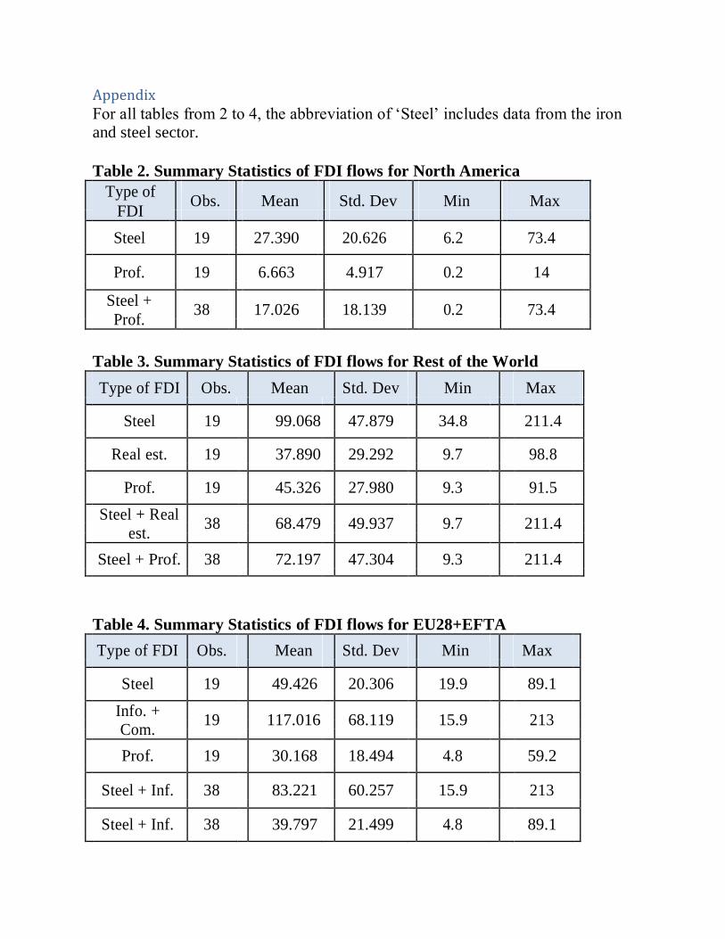
For all tables from 2 to 4, the abbreviation of ‘Steel’ includes data from the iron and steel sector.

Table 2. Summary Statistics of FDI flows for North America

Type of Obs.

Mean

Std. Dev

Min

Max

FDI

Steel 19 27.390 20.626 6.2 73.4

Prof. 19 6.663 4.917 0.2 14

Steel + 38

17.026

18.139

0.2

73.4

Prof.

Table 3. Summary Statistics of FDI flows for Rest of the World

Type of FDI Obs. Mean Std. Dev Min Max

Steel 19 99.068 47.879 34.8 211.4

Real est. 19 37.890 29.292 9.7 98.8

Prof. 19 45.326 27.980 9.3 91.5

Steel + Real 38

68.479

49.937

9.7

211.4

est.

Steel + Prof. 38 72.197 47.304 9.3 211.4

Table 4. Summary Statistics of FDI flows for EU28+EFTA

Type of FDI Obs. Mean Std. Dev Min Max

Steel 19 49.426 20.306 19.9 89.1

Info. + 19

117.016

68.119

15.9

213

Com.

Prof. 19 30.168 18.494 4.8 59.2

Steel + Inf. 38 83.221 60.257 15.9 213

Steel + Inf. 38 39.797 21.499 4.8 89.1

30

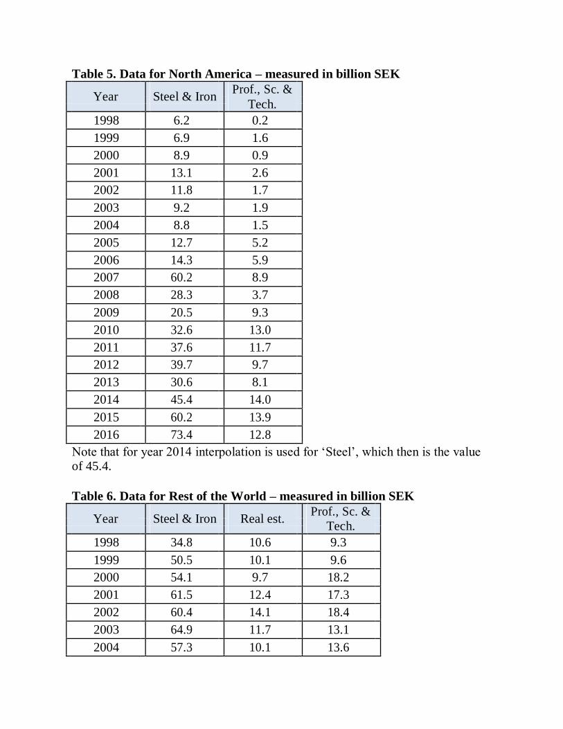
Table 5. Data for North America – measured in billion SEK

Year

Steel & Iron

Prof., Sc. &

Tech.

1998 6.2 0.2

1999 6.9 1.6

2000 8.9 0.9

2001 13.1 2.6

2002 11.8 1.7

2003 9.2 1.9

2004 8.8 1.5

2005 12.7 5.2

2006 14.3 5.9

2007 60.2 8.9

2008 28.3 3.7

2009 20.5 9.3

2010 32.6 13.0

2011 37.6 11.7

2012 39.7 9.7

2013 30.6 8.1

2014 45.4 14.0

2015 60.2 13.9

2016 73.4 12.8

Note that for year 2014 interpolation is used for ‘Steel’, which then is the value of 45.4.

Table 6. Data for Rest of the World – measured in billion SEK

Year

Steel & Iron

Real est.

Prof., Sc. & Tech.

1998 34.8 10.6 9.3

1999 50.5 10.1 9.6

2000 54.1 9.7 18.2

2001 61.5 12.4 17.3

2002 60.4 14.1 18.4

2003 64.9 11.7 13.1

2004 57.3 10.1 13.6

2005 56.8 16.5 45.1

2006 64.6 11.5 44.9

2007 116.7 50.5 81.6

31

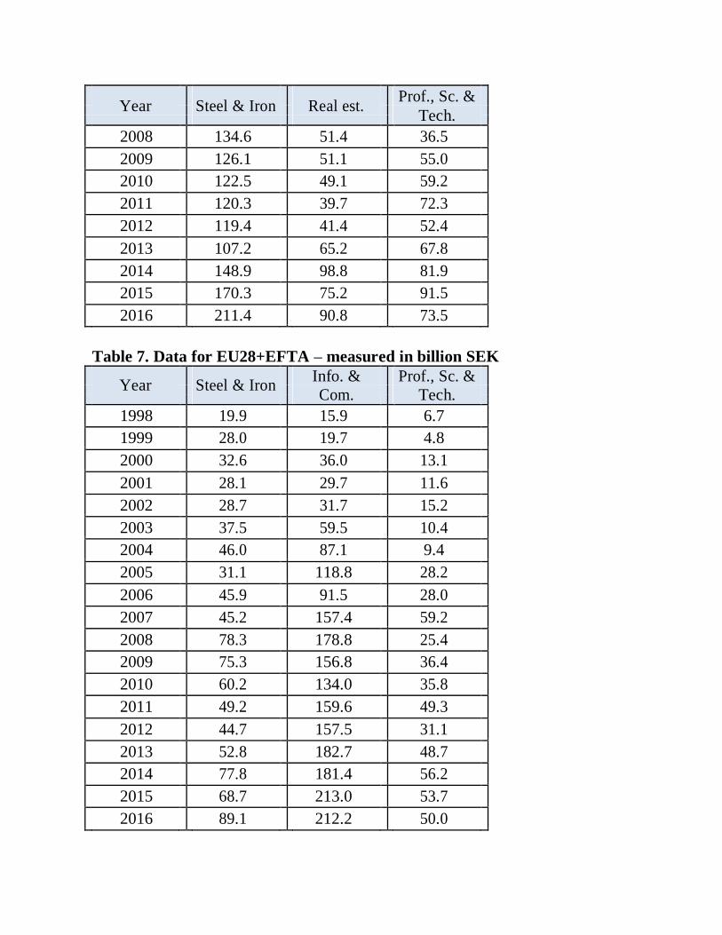
Year

Steel & Iron

Real est.

Prof., Sc. &

Tech.

2008 134.6 51.4 36.5

2009 126.1 51.1 55.0

2010 122.5 49.1 59.2

2011 120.3 39.7 72.3

2012 119.4 41.4 52.4

2013 107.2 65.2 67.8

2014 148.9 98.8 81.9

2015 170.3 75.2 91.5

2016 211.4 90.8 73.5

Table 7. Data for EU28+EFTA – measured in billion SEK

Year

Steel & Iron

Info. & Prof., Sc. &

Com.

Tech.

1998 19.9 15.9 6.7

1999 28.0 19.7 4.8

2000 32.6 36.0 13.1

2001 28.1 29.7 11.6

2002 28.7 31.7 15.2

2003 37.5 59.5 10.4

2004 46.0 87.1 9.4

2005 31.1 118.8 28.2

2006 45.9 91.5 28.0

2007 45.2 157.4 59.2

2008 78.3 178.8 25.4

2009 75.3 156.8 36.4

2010 60.2 134.0 35.8

2011 49.2 159.6 49.3

2012 44.7 157.5 31.1

2013 52.8 182.7 48.7

2014 77.8 181.4 56.2

2015 68.7 213.0 53.7

2016 89.1 212.2 50.0

All data is retrieved from Statistiska Centralbyrån (SCB) through personal

communication (e-mail) via Rickard Rens.

32