BPEA Conference Drafts, March 8–9, 2018

Is automation labor-displacing? Productivity growth, employment, and the labor share

David Autor, Massachusetts Institute of Technology

Anna Salomons, Utrecht University

Conflict of Interest Disclosure: David Autor is a trustee and board member for the Urban Institute,

and codirector of the Labor Studies Program at the National Bureau of Economic Research. Autor

received financial support for this work from the IBM Open Collaboration Research award

program, Schmidt Family Foundation, and Smith Richardson Foundation. Anna Salomons

received financial support for this work from the Netherlands Organization for Scientific Research

through the Innovational Research Incentives Scheme Veni research grant program. With the

exception of the aforementioned, the authors did not receive financial support from any firm or

person for this paper or from any firm or person with a financial or political interest in this paper.

With the exception of the aforementioned, they are currently not officers, directors, or board

members of any organization with an interest in this paper. No outside party had the right to review

this paper before circulation.

Is Automation Labor-Displacing?

Productivity Growth, Employment, and the Labor Share

February 27, 2018

David Autor

Anna Salomons1

Abstract

Is automation a labor-displacing force? This possibility is both an age-old concern and at the heart

of a new theoretical literature considering how labor immiseration may result from a wave of

‘brilliant machines,’ which is in part motivated by declining labor shares in many developed

countries. Comprehensive evidence on this labor-displacing channel is at present limited. Using

the recent model of Acemoglu and Restrepo (2018b) as an analytical frame, we first outline the

various channels through which automation impacts labor´s share of output. We then turn to

empirically estimating the employment and labor share impacts of productivity growth—an

omnibus measure of technological change—using data on 28 industries for 18 OECD countries

since 1970. Our main findings are that although automation—whether measured by Total Factor

Productivity growth or instrumented by foreign patent flows or robot adoption—has not been

employment-displacing, it has reduced labor’s share in value-added. We disentangle the channels

through which these impacts occur, including: own-industry effects, cross-industry input-output

linkages, and final demand effects accruing through the contribution of each industry’s

productivity growth to aggregate incomes. Our estimates indicate that the labor share-displacing

effects of productivity growth, which were essentially absent in the 1970s, have become more

pronounced over time, and are most substantial in the 2000s. This finding is consistent with

automation having become in recent decades less labor-augmenting and more labor-displacing.

1 Autor: MIT Department of Economics, Cambridge, MA 02142 (dautor@mit.edu); Salomons: Utrecht University

School of Economics, 3584 EC Utrecht, The Netherlands; & Technology & Policy Research Initiative, Boston

University (a.m.salomons@uu.nl). Paper prepared for the Brookings Papers on Economic Activity conference, March

2018. We thank Daron Acemoglu, Uwe Blien, Janice Eberly, Maarten Goos, John Haltiwanger, Richard Rogerson,

James Stock, and Xianjia Ye for valuable input that improved the paper. We thank Daron Acemoglu, Georg Graetz,

Guy Michaels, and Pascual Restrepo for sharing harmonized code on penetration of industrial robotics. And we think

Pian Shu for sharing data on approved patent applications by industry and year of filing. Autor acknowledges

funding from IBM Higher Education, Schmidt Sciences, and the Smith-Richardson Foundation. Salomons

acknowledges funding from the Netherlands Organisation for Scientific Research.

1

Introduction

One of the central stylized facts of modern macroeconomics, immortalized by Kaldor (1961),

is that during a century of unprecedented technological advancement in transportation,

production, and communication, labor’s share of national income remained roughly constant

(Jones and Romer, 2010). This empirical regularity, which Keynes (1939) deemed “a bit of a

miracle,” has provided economists—though not the lay public—with grounds for optimism

that, despite seemingly limitless possibilities for labor-saving technological progress,

automation need not make labor irrelevant as a factor of production. Indeed, mainstream

macroeconomic literature often takes as given that labor’s share of national income is constant

and asks what economic dynamics enforce this constancy.2

But several recent developments have eroded economists’ longstanding confidence in this

constancy. One is a widely-shared view that recent and incipient breakthroughs in artificial

intelligence and dexterous, adaptive robotics are profoundly shifting the terms of human vs.

machine comparative advantage. Observing these advances, numerous scholars and popular

writers anticipate the wholesale elimination of a vast set of currently labor-intensive and

cognitively demanding tasks, leaving an ever-diminishing set of activities in which labor adds

significant value (Brynjolfsson and McAfee, 2014; Ford, 2017; Frey and Osborne, 2017).

A widely noted empirical regularity that lends credence to this narrative is that labor’s share

of national income has in recent decade fallen in many nations, a trend that may have become

more pronounced in the 2000s (e.g., Elsby, Hobijn and Sahin, 2013; Karabarbounis and Neiman,

2013; Piketty 2014; Autor et al. 2017b; Dao et al. 2017). Reviewing an array of within- and cross-

country evidence, Karabarbounis and Neiman (2014) argue that labor’s falling share of value-

added is caused by a steep drop in the quality-adjusted equipment prices of Information and

Communication Technologies (ICT) relative to labor. Though Karabarbounis and Neiman’s

work is controversial in that it implies an aggregate capital-labor substitution in excess of

2 Ngai and Pissarides (2007) and Acemoglu and Guerrieri (2012) formulate models in which ongoing unbalanced

productivity growth across sectors (as per Baumol 1967) can nevertheless yield a balanced growth path for labor and

capital shares.

2

unity—which is a non-standard assumption in this literature—their work has lent empirical

weight to the hypothesis that computerization may erode labor demand.3

Indeed, while a fall in the labor share is ruled out by design in most canonical

macroeconomic models (e.g., Ngai and Pissarides 2007), recent literature revisits this

assumption, offering models where labor displacement is one potential outcome. For example,

Sachs and Kotlikoff (2012) and Berg et al. (2017) write down an overlapping-generation models

in which rapid labor-saving technological advances generate short-run gains for skilled workers

and capital owners, but in the longer run, immiserate those who are not able to invest in

physical or human capital. Acemoglu and Restrepo (forthcoming and 2018b) consider models in

which two countervailing economic forces determine the evolution of labor’s share of income:

the march of technological progress, which gradually replaces ‘old’ tasks, reducing labor’s share

of output and possibly diminishing real wages; and endogenous technological progress that

generates novel labor-demanding tasks, potentially reinstating labor’s share. The interplay of

these forces can—but need not necessarily—yield a balanced growth path wherein the

reduction in labor scarcity due to task replacement induces endogenous creation of new labor-

using job tasks, thus restoring labor’s share.4

The current paper assesses evidence for labor displacement, which in our terminology

means productivity-enhancing technological advances that reduce labor’s share of aggregate

output. As our formal model below clarifies, labor displacement need not imply a decline in

3 Although such a relative capital price decline will have no effect on factor shares if production technologies are

Cobb-Douglas, there will be a decline in the labor share if the capital-labor elasticity of substitution is greater than

one (a proposition for which Karabarbounis and Neiman find some evidence). Dao et al. (2017) present cross-country

evidence from both developed and developing countries that machine-labor substitution, stemming from Routine-

Replacing Technical Change (RRTC), contributes to a reduction in labor’s share through falling middle-skilled labor

demand. Analyzing data for both Europe and the U.S., Autor et al. (2017b) conclude that the falling labor share is

more likely accounted for by the rise of ‘winner take most’ competition rather than direct capital-labor or trade-labor

substitution—though this change in the nature of competition may itself be a technologically induced phenomenon.

4 Susskind (2017) develops a model in which labor is ultimately immiserated by the asymptotic encroachment of

automation into the full spectrum of work tasks. A key distinction between Acemoglu and Restrepo (forthcoming)

and Susskind (2017) is that, in the latter model, falling labor scarcity does not spur the endogenous creation of new

labor-using tasks or labor-complementing technologies, thus guaranteeing labor immiseration. The conceptual

frameworks of both papers build on Zeira (1998) and Autor, Levy, and Murnane (2003, ALM), which feature models

in which advancing automation reduces labor’s share by substituting machines (or computers) for workers in a

subset of activities (which ALM designate as ‘tasks’).

3

employment, hours, or wages. Rather, it simply requires that the wagebill—that is, the product

of hours of work and wages per hour—rises less rapidly than does value-added. As highlighted

in Acemoglu and Restrepo (forthcoming and 2018b), a natural mechanism through which this

could occur is via task-replacing technological change, meaning technological advances that

shift production tasks directly from capital to labor, thereby reducing labor’s share of output.

This direct negative direct effect of automation on labor’s share may be partly or fully offset by a

several countervailing forces—also spurred by automation—including rising productivity,

capital deepening, and the introduction of new labor-using tasks. Nevertheless, the notion that

automation directly reduces labor’s share of output does not feature in canonical

macroeconomic models that exhibit a balanced growth path. As will become apparent, our

results are difficult to square with the simplest variants of such models.

Our work contributes to a growing literature assessing whether rapid automation has

served to dampen aggregate labor demand or overall wage growth. Focusing on the first half of

the twentieth century, Alexopoulos and Cohen (2016) find that positive technology shocks

raised productivity and lowered unemployment in the United State between 1909 and 1949.

Using contemporary European data, Gregory, Salomons, and Zierahn (2016) test whether

Routine-Replacing Technical Change (RRTC) has reduced employment overall across Europe

and find that while RRTC has reduced middle-skill employment, this employment reduction is

more than offset by compensatory product demand and local demand spillovers.5 In work

closely related to the current paper, Dao et al. (2017) analyze sources of the trend decline in

labor share in a panel of 49 emerging and industrialized countries. Using cross-country and

cross-sector variation in the prevalence of occupations potentially susceptible to automation (as

per Autor and Dorn, 2013), Dao et al. find that countries and sectors initially more specialized in

routine-intensive activities have seen a larger decline in labor share, consistent with the

5 Focusing not on employment but on sectoral and aggregate outputs, Nordhaus (2015) presents evidence that

industrialized economies are not approaching an inflexion point at which technological advances generate a sharp

and sustained acceleration of economic growth.

4

possibility of labor displacement.6 Concentrating on industrial robotics, arguably the leading

edge of workplace automation, Graetz and Michaels (2015) conclude that industry-level

adoption of industrial robots has raised labor productivity, increased value-added, augmented

worker wages, had no measurable effect on overall labor hours, and modestly shifted

employment in favor of high-skill workers within EU countries. Conversely, using the same

underlying industry-level robotics data but applying a cross-city design within the U.S.,

Acemoglu and Restrepo (2017) present evidence that U.S. local labor markets that were

relatively exposed to industrial robotics experienced differential falls in employment and wage

levels between 1990 and 2007.

Akin to Graetz and Michaels (2015) and Dao et al. (2017), the current paper applies

harmonized cross-country and cross-industry data to explore the relationship between

technological change and labor market outcomes. Our work advances this literature in four

dimensions. First, rather than focusing exclusively on specific measures of technological

adoption or susceptibility (e.g., robotics, routine task replacement), we focus initially on an

omnibus measure of technological progress: total factor productivity growth or TFP (Solow,

1956). Using TFP as our baseline measures potentially overcomes the challenge for consistent

measurement posed by the vast heterogeneity of innovation across sectors and periods.

TFP also has significant limitations as a measure of technological progress, however: since it

is ultimately a regression residual, its relationship to any specific technological advance is

unspecified; moreover, estimates of TFP may be confounded with business cycle effects,

industry trends, and cross-industry differences in cyclical sensitivity (Basu and Fernald, 2001). 7

A second contribution of the current paper is to address both concerns. Complementing the

estimates using reported TFP growth, we instrument or proxy for industry-level productivity

growth with specific measures of technology and innovation, including industry-level

patenting, ICT investment, and robot density. To purge the potential cyclicality of TFP, our

6 Using an analogous approach, Michaels, Natraj, and Van Reenen (2014) find that ICT adoption is predictive of

within-sector occupational polarization in a country-industry panel sourced from EUKLEMS covering 11 countries

observed over 25 years.

7 Moses Abramovitz (1956) famously declared the TFP residual, “a measure of our ignorance.”

5

main specifications include business cycle by industry by country fixed effects, which non-

parametrically absorb differential sensitivity of industry measures of productivity to business

cycle variation. As a second step, we perform a set of robustness checks that use exclusively

low-frequency TFP variation, thus leveraging secular shifts in TFP while purging cyclical

variation.

A longstanding conceptual issue pervading this literature, and one which this paper seeks

to overcome, is the tension between using microeconomic variation for identification while

attempting to speak to macroeconomic outcomes. This concern applies here because we study

the relationship between productivity growth, innovation, and labor displacement using cross-

country-industry, over-time variation. As theory makes clear, however, there is no direct

mapping between the evolution of productivity and labor demand at the industry level and the

evolution of aggregate labor demand. For example, Ngai and Pissarides (2007) show that

uneven rates of productivity growth across industries—which may spur substantial changes in

employment across sectors as per Baumol (1967)—need not imply any deviation from an

aggregate balanced growth path under some specifications of preferences.8 Thus, at face value,

the industry-level relationships that we estimate are not necessarily informative about aggregate

outcomes of interest.

Recognizing this concern, a third contribution of this paper is to incorporate two key micro-

macro linkages that, in combination with the industry-level estimates, allow us to make broader

statements about aggregate effects. The first link applies harmonized data enumerating cross-

industry input-output linkages to trace the effects of productivity growth in each industry to

outcomes occurring in customer industries and in supplier industries—that is, industries for

which the originating industry is upstream and downstream in the production chain,

8 Specifically, the intertemporal elasticity of substitution must be unity, the elasticity of substitution across

consumption goods must be non-unity, and the rate of output growth in the intermediates good sector

(manufacturing) must be constant. It bears note that Ngai-Pissarides specify Cobb-Douglas production functions for

each sector, meaning that labor’s share is unchanging within each sector. Our far more stylized conceptual model

relaxes this constraint, while our analysis suggests that this relaxation is required.

6

respectively.9 The second link we explore is between aggregate economic growth and sectoral

labor demand. Recognizing that productivity growth in each industry augments aggregate

income and hence indirectly raises final demand, we estimate the elasticity of sectoral demands

emanating from aggregate income growth and then apply our TFP estimates to infer the

indirect contribution of each industry’s productivity growth to final demand. Our net estimates

of the impact of productivity growth and innovation on outcomes of interest therefore sum over

(1) direct industry-level effects; (2) indirect upstream and downstream effects in linked sectors;

and (3) final demand effects accruing through the effect of productivity growth on aggregate

value-added.

A final contribution of the paper is that, by leveraging more than four decades of

harmonized industry by country data, we can assess not only whether productivity growth and

innovation appear to be labor-displacing, but whether this relationship has shifted over

successive decades. In point of fact, we find distinctly different patterns between the first

decade in our sample, the 1970s, and the three decades that follow.

The paper is structured as followed. We first lay out a simple ‘task’ model based on

Acemoglu and Restrepo (2018a) that formalizes the notion of labor displacement, clarifies how

it may be distinguished from a conventional neoclassical setting featuring balanced growth, and

discusses the mapping from this stylized conceptual framework to the empirical exercise that

follows.

After summarizing the data and measurement framework in Section 2, Section 3 of the

paper presents our main estimates for the effect of productivity growth (measured initially by

TFP) on labor input, value-added, and labor’s share of value-added, accounting for both direct

own-industry effects, and for indirect effects operating through input-output linkages and

aggregate demand. Consistent with first principles, we find that TFP shocks raise own-industry

9 Specifically, we pair the EU KLEMS with tables from the World Input-Output Databse (Timmer, 2009 and 2015) to

calculate Leontief inverse weighting matrix that traces the full effect of shocks in each given sector to those in

customer and supplier sectors, accounting not only for first-order effects but the full set of dependencies emanating

from the fact that, for example, customer industries also buy input from additional industries that are suppliers to or

customers of the industry experiencing the initial shock. Our analysis follows many recent works exploiting these

linkages to study the propagation of trade and technology shocks (Acemoglu et al. 2016; Pierce and Schott, 2016;

Acemoglu, Akcigit and Kerr, 2017).

7

output, increase value-added, and lower output prices. While hours of labor input fall in sectors

undergoing relatively rapid productivity growth, we find that the indirect effects of own-sector

TFP growth robustly offset the reduction in labor hours in advancing sectors. Specifically,

hours-reducing productivity growth in supplier industries spurs countervailing hours

expansions in customer industries; and the cumulative contribution of each sector’s productive

growth to aggregate value-added, combined with a strongly positive aggregate elasticity of

hours with respect to value-added, further raises the estimated net effect of industry-level

productivity gains on aggregate labor hours. 10

This pattern of falling labor input in advancing industries with countervailing gains in labor

input in (relatively) non-advancing industries is consistent with models of structural change in

which labor is displaced from ‘progressive’ to ‘stagnant’ sectors (Baumol, 1967; Ngai and

Pissarides, 2007).11 But our next set of results do not support the canonical version of this story

in which labor input falls in advancing industries because industry output demand is inelastic.

Contrary to this reasoning, we estimate that industry output demand is on average highly

elastic, which would typically imply no net negative effect of productivity growth on industry-

level labor demand. We find instead that labor’s share of value-added falls significantly in

advancing industries, which we refer to as labor displacement. This labor displacement is

inconsistent with models of structural change that assume an underlying Cobb-Douglas

production structure in each industry.

These industry-level labor displacement findings would be less interesting, however, if

industry-level productivity growth spurred offsetting gains in labor share elsewhere in the

economy, i.e., through input-output linkages and aggregate demand effects, as occurs with

hours of labor input. We find that these countervailing effects are present in the data, but they

are far less than fully offsetting: labor-displacing productivity growth in upstream supplier

10 As outlined in Acemoglu, Akcigit, and Kerr (2017), in a canonical Cobb-Douglas economy, productivity innovations

occurring in a given sector should raise output in its customer sectors but should have no measurable effect on

output in its supplier sectors due to offsetting quantity and price effects. Perhaps surprisingly, our analysis supports

this prediction.

11 As Ngai and Pissarides (2007) clarify, this prediction requires that the outputs of these sectors are gross

complements in final consumption. If they are instead gross substitutes, labor flows towards progressive sectors.

8

industries spurs offsetting gains in labor share in customer industries, but this countervailing

effect is only half as large as the estimated own-industry effect. Meanwhile, we detect no

positive relationship between growth in aggregate value-added and growth in labor share,

meaning that although industry-level productivity growth does augment aggregate growth,

this does not affect labor’s share of value-added.

Putting these pieces together, we estimate in Section 4 that productivity growth—measured

by TFP or proxied by various direct measures of technological advance—has served to reduce

labor’s share of value-added in aggregate. Notably, this negative relationship was not always

present, even within our four-decade analytic window. Our estimates suggest that productivity

growth and innovation had virtually no net labor share-displacing effect during the 1970s. This

relationship turned negative (labor-displacing) in the 1980s and 1990s, and it becomes more

negative still in the 2000s.

To address concerns about the potential endogeneity of industry-level TFP, Section 5

employs two direct measures of industry-level technological advances that serve as

instrumental variables for TFP: patent flows and the penetration of industrial robots. Both sets

of variables prove to be significant predictors of industry-level TFP growth. And using each

source of variation, we find that automation has become increasingly labor-displacing in recent

decades, both at the industry level and in aggregate. Not surprisingly, the estimates for

industrial robots are somewhat weaker given that the penetration of industrial robotics is

relatively recent and is concentrated in a subset of industries.

In the conclusion, we briefly consider the interpretation of our findings, focusing in

particular on the relationship between the industry-level and aggregate outcomes, which are

observed in our data, and the underlying firm-level dynamics that may contribute to these

outcomes.

1. Labor market consequences of automation: A task framework

To formalize the notion of labor-displacing technological change that frames our thinking,

we sketch a simple task-based framework developed in Acemoglu and Restrepo (2018b), which

in turn builds on Zeira (1998), Autor, Levy, Murnane (2003) and Acemoglu and Autor (2011).

9

We assume that aggregate output is produced by combining the services of a unit measure

of tasks 𝑥 ∈ [𝑁 − 1,𝑁] according to the following Cobb-Douglas (unit elasticity) aggregator:

𝑌 = ∫ ln𝑦(𝑥)𝑑𝑥 𝑁

𝑁−1

, (1)

where 𝑌 denotes aggregate output and 𝑦(𝑥) is the output of task 𝑥.

All tasks can be performed by labor, ℓ(𝑥). If a task has been technologically automated, it

can also be performed by machines 𝓂(𝑥). At a point in time, tasks 𝑥 ∈ [𝑁 − 1, 𝐼] are

technologically automated, while the remainder are not. We further assume that labor

and machines are perfect substitutes in technologically automated tasks, although their

relative productivity/costs at these tasks may differ. Services of task 𝑥 are equal to:

𝑦(𝑥) = {𝛼𝐿𝛾𝐿(𝑥)ℓ(𝑥) + 𝛼𝑀𝛾𝑀(𝑥)𝓂(𝑥) if 𝑥 ∈ [𝑁 − 1, 𝐼]

𝛼𝐿(𝑥)𝛾𝐿ℓ(𝑥) if 𝑥 ∈ [𝐼, 𝑁]

(2)

Here, 𝛼𝐿 and 𝛼𝑀 are efficiency terms that affect the productivity of labor and capital,

respectively, at each task to which they are assigned. Meanwhile, 𝛾𝐿(𝑥) and 𝛾𝑀(𝑥) are task-

specific efficiency terms. The task-specific efficiency of labor in task 𝑥 is 𝛾𝐿(𝑥) while,

analogously, 𝛾𝑀(𝑥) is the task-specific efficiency of machines in task 𝑥 (where 𝑥 ≤ 𝐼). A key

assumption is that 𝛾𝐿(𝑥)/𝛾𝑀(𝑥) is increasing in 𝑥, meaning labor has comparative advantage in

higher-indexed tasks.

The threshold 𝐼 denotes the frontier of automation possibilities. This threshold can rise over

time due to advancements in automation, artificial intelligence, industrial robotics, etc. For

expositional simplicity, we assume that both the supply of labor, 𝐿, and the supply of machines,

𝑀, are fixed and inelastic, though these assumptions have no bearing on our empirical analysis.

This simple model admits four distinct forms of technological change with a rich set of

empirical implications: (1) conventional factor-augmenting technical changes, corresponding to

a rise in either 𝛼𝐿 or 𝛼𝑀; (2) extensive margin (labor-displacing) technical changes,

corresponding to a rise 𝐼; (3) intensive margin capital- or labor-augmenting technical changes,

corresponding to a rise in 𝛾𝐿(𝑥) or 𝛾𝑀(𝑥) for some subset of tasks in the interval [𝑁 − 1,𝑁]; and

(4) task-creating technical change, corresponding to a rise in 𝑁. After solving for the model’s

10

equilibrium, we consider the implications of each type of technological change for labor

demand.

1.1. Labor market equilibrium

In equilibrium, firms choose the cost-minimizing way of producing each task and labor and

capital markets to clear. Denote the equilibrium wage rate by 𝑊 and the equilibrium capital

rental rate by 𝑅. Following Acemoglu and Restrepo (2018b), we impose the assumption that

𝛼𝐿𝛾𝐿(𝑁)

𝛼𝑀𝛾𝑀(𝑁 − 1)>𝑊

𝑅> 𝛼𝐿𝛾𝐿(𝐼)

𝛼𝑀𝛾𝑀(𝐼) (A1)

The first of these inequalities implies that the introduction of new tasks (a rise in 𝑁) will raise

aggregate output.12 The second inequality implies that the all tasks in the interval [𝑁 − 1, 𝐼] will

be performed by machines. 13 Assumption A1 is not innocuous in that it implies that the wage

ratio is neither so high that new task creation lowers output nor so low so that some tasks that

are technologically automated are nevertheless performed by labor. In reality, the empirical

analysis in our paper is silent on new task creation, so the first condition has no bearing. The

second condition is only made for expositional convenience, and it is relaxed in Acemoglu and

Autor (2011).

As formally demonstrated in the Appendix (Section 8), output (GDP) in the equilibrium in

this model can be expressed as

𝑌 = 𝐵 (

𝛼𝑀𝑀

𝐼 −𝑁 + 1)𝐼−𝑁+1

(𝛼𝐿𝐿

𝑁 − 𝐼)𝑁−𝐼

(3)

where

𝐵 = exp(∫ ln𝑦𝑀(𝑥)𝑑𝑥 𝐼

𝑁−1

+∫ ln𝑦𝑀(𝑥)𝑑𝑥 𝑁

𝐼

). (4)

Notice that eqn. (3) is a conventional Cobb-Douglas production function, where capital’s share

of output is given by the exponent (𝐼 − 𝑁 + 1) and labor’s share of output is given by the

12 Formally, this inequality says that the ratio of labor productivity in a newly-introduced task to capital productivity

in a newly-eliminated task is greater than the wage/rental ratio, so output rises.

13 Thus, 𝐼 is a ‘hard’ technical constraint on automation rather than a no-arbitrage condition between capital and

labor.

11

complement (𝑁 − 𝐼). The expression for the multiplier 𝐵 on the Cobb-Douglas aggregator in (3)

is a weighed sum of the relevant labor and capital efficiency terms (see eqn. 4). Conventionally,

𝐵 corresponds to Total Factor Productivity (TFP), i.e., the Solow residual. TFP can shift in this

model because one or both of the efficiency terms (𝑦𝑀, 𝑦𝐿) rises or because tasks are reallocated

from labor to capital (a rise in 𝐼) or from capital to labor (a rise in 𝑁). Thus, distinct from the

canonical Solow model, TFP growth in this setting is not Hicks-neutral if it stems from

movements in either 𝐼 or 𝑁.

The demand for labor can be written as

𝑊 = (𝑁 − 𝐼)𝑌

𝐿 (5)

This is again a familiar Cobb-Douglas expression, with the marginal product of labor equal to

the average product of labor equal multiplied by the exponent on labor in the production

function. We can rearrange this expression to obtain labor’s share of output as

𝑆𝐿 =𝑊𝐿

𝑌= 𝑁 − 𝐼 (6)

We next consider how several distinct varieties of technological change affect the equilibrium of

this model.

1.2. Factor augmenting technological change

In canonical production models, technological change is factor-augmenting. Factor-

augmenting change is also present in the current model. A rise in either 𝛼𝐿 or 𝛼𝑀—signifying

labor and capital-augmenting technical change, respectively—increases wages and output, with

no effect on the labor share:

𝑑 ln𝑊

𝑑 ln 𝛼𝐿=𝑑 ln(𝑌/𝐿)

𝑑 ln𝛼𝐿= (𝑁 − 𝐼)𝑑 ln𝛼𝐿 > 0,

and similarly,

𝑑 ln𝑊

𝑑 ln 𝛼𝑀=𝑑 ln(𝑌/𝐿)

𝑑 ln𝛼𝑀= (𝐼 − 𝑁 + 1)𝑑 ln𝛼𝑀 > 0.

with 𝑑lnY 𝑑ln𝛼𝐿 =⁄ 𝑑 ln 𝑌 𝑑ln𝛼𝑀 =⁄ 1 and 𝑑𝑆𝐿 𝑑𝛼𝐿⁄ = 𝑑𝑆𝐿 𝑑𝛼𝑀⁄ = 0. Thus, although the model

admits unconventional technological channels, it fully encompasses the conventional ones.

12

1.3. Extensive margin (labor-displacing) technical change

Consider a technological advance that extends the range of tasks that are technologically

automated—that is, it increases 𝐼. This advance has two countervailing effects on wages, seen in

the expression below:

𝑑 ln𝑊

𝑑𝐼=𝑑 ln(𝑁 − 𝐼)

𝑑𝐼+𝑑 ln(𝑌 𝐿⁄ )

𝑑𝐼 (7)

The first term to the right of the equal sign reflects the labor-displacing effect of extensive

margin technological change. Holding output constant, extensive margin technological change

reduces labor’s share of output and hence wages. Since capital is more cost-effective than labor

in the threshold task (Assumption A1), however, extensive margin technological change also

raises output.

These countervailing effects may be seen by expanding eqn. (7):

𝑑 ln𝑊

𝑑𝐼= [−

1

𝑁 − 𝐼] + [ln (

𝑊

𝛼𝐿𝛾𝐿(𝐼)) − ln (

𝑅

𝛼𝑀𝛾𝑀(𝐼))] (8)

The first bracketed term in eqn. (8) is the displacement effect. It is negative since extensive margin

technical change reallocates tasks from labor to capital (specifically, 𝑑𝑆𝐿 𝑑𝐼⁄ = −1, where 𝑆𝐿 is

labor share of GDP). The second term, corresponding to rising productivity, is unambiguously

positive by Assumption A1: since capital is more cost-effective than labor in newly automated

tasks14, automation raises output, a share of which is paid to labor.

This productivity effect may in turn operate through two channels, one direct and one

indirect. The first (direct) effect is that automation may increase labor demand in non-

automated tasks in the industry where automation is taking place. We refer to this channel as

the ‘Uber’ effect, i.e., a technological improvement that both raises labor productivity and

employment in the affected sector. Additionally or alternatively, productivity growth in a

technologically advancing industry may raise labor demand in other industries. This indirect

effect may occur because rising productivity raises consumer incomes and boosts final

demand—what we call the ‘Walmart’ effect—or because automation lowers input costs to

downstream customer industries, leading to output and employment growth in these

14 Were this not the case, newly technologically automated tasks would nevertheless be performed by labor rather

than machines.

13

downstream sectors—what we call the ‘Costco’ effect. Formally, these indirect effects (Walmart,

Costco) exist outside of our simple model since the model contains only one sector. These

distinct channels are, however, empirically distinguishable, and we will explore them below.

A notable implication of eqn. (8) is that although extensive margin technological change

necessarily raises GDP, it need not raise wages due to its countervailing effects on productivity

and on labor’s share of output. As Acemoglu and Restrepo (2018b) emphasize, the net wage

effect is more likely to be positive when capital is highly productive at the tasks that are newly

automated (e.g., telephones replacing telegraphs—dramatically raising productivity while

reducing labor requirements). Conversely, the wage effects may be negative when labor-

replacing technologies have minimal productivity advantages over the workers they displace,

e.g., self-checkout scanners at grocery stores replacing checkout clerks, or computerized phone

menus replacing human customer service assistants. In the extreme case where capital is

negligibly more productive at the threshold task than labor (ln(𝑊 𝛼𝐿𝛾𝐿(𝐼)⁄ ) ≈ ln(𝑅 𝛼𝑀𝛾𝑀(𝐼)⁄ ),

technological change reallocates income from labor to capital with essentially no effect on

productivity, meaning that wages fall.

1.4. Intensive margin technical change, capital deepening, and elastic capital supply

While technological change along the extensive margin has an ambiguous effect on wages,

technological change that boosts productivity in already-automated tasks necessarily raises labor

demand. For example, if capital efficiency is initially identical in all technologically automated

tasks (𝛾𝑀(𝑥) = 𝛾𝑀), and if 𝛾𝑀 rises with no change in 𝐼, then

𝑑 ln𝑊 = 𝑑 ln𝑌 𝐿⁄ = (𝐼 − 𝑁 + 1)𝑑 ln 𝛾𝑀 > 0.

That is, wages rise.

Similarly, a fall in the capital rental rate 𝑅—reflecting capital deepening—increases wages

(seen in eqn. 8). In the limit where capital is perfectly elastically supplied (𝑅 is fixed), the

productivity gains from technological change accrue exclusively to labor.15

15 The positive wage effects of each of these three channels—intensive margin technical change, capital deepening,

and elastic capital supply—reflect q-complementarity. Because capital and labor are q-complements in production, a

rise in the quantity or quality of either raises the marginal product of the other.

14

1.5. Creation of new tasks

A final channel (unconventional) channel by which technological change may affect output

and wages in this model is through the creation of new tasks in which labor has comparative

advantage—that is, a rise in 𝑁. These new tasks might include novel labor-using activities (e.g.,

computer programming, laparoscopic surgery) or new variations of existing labor-using tasks

(e.g., welding instead of riveting).

The effect of a rise in 𝑁 on output and wages can be written as:

𝑑 ln𝑊

𝑑𝑁=𝑑 ln𝑌/𝐿

𝑑𝑁+

1

𝑁 − 𝐼

= [ln (𝑅

𝛼𝑀𝛾𝑀(𝑁 − 1)) − ln (

𝑊

𝛼𝐿𝛾𝐿(𝑁))] + [

1

𝑁 − 𝐼] .

(9)

In this expression, the first bracketed term reflects the rise in labor productivity stemming from

the creation of new tasks, which is necessarily positive under Assumption A1. The second

bracketed term reflects the gain in labor’s share of income as tasks are reallocated from

machines to workers.16

Combining equations (7) and (9), we can write the total effect of task-replacing technical

change and new task creation on wages as

𝑑 ln𝑊 = [ln (𝑅

𝛼𝑀𝛾𝑀(𝑁 − 1)) − ln (

𝑊

𝛼𝐿𝛾𝐿(𝑁))] 𝑑𝑁

+ [ln (𝑊

𝛼𝐿𝛾𝐿(𝐼)) − ln (

𝑅

𝛼𝑀𝛾𝑀(𝐼))] 𝑑𝐼 + [

1

𝑁 − 𝐼] (𝑑𝑁 − 𝑑𝐼).

(10)

This expression underscores that for labor’s share to remain constant and wages to rise in

tandem with productivity, task displacement and task creation must proceed at the same pace.

In that case, 𝑑𝑆𝐿 = 𝑑𝑁 − 𝑑𝐼 = 0, and eqn. (10) reduces to

𝑑 ln𝑊 = [ln (𝛼𝐿𝛾𝐿(𝑁)

𝛼𝑀𝛾𝑀(𝑁 − 1)) − ln (

𝛼𝐿𝛾𝐿(𝐼)

𝛼𝑀𝛾𝑀(𝐼))]𝑑𝐼 > 0, (11)

which is unambiguously positive.

16 This latter term may appear an artifact of the assumption that there is a unit measure of tasks, so the creation of

new labor-using tasks implies the elimination of an equal measure of technologically-automated tasks. However,

even if old tasks were not eliminated, the creation of new labor-using tasks would raise labor’s share of output. In

that case, the derivative 𝑑𝑆𝐿 𝑑𝑁⁄ would be equal to 1 rather than 1 (𝑁 − 𝐼)⁄ , which exceeds 1.

15

1.6. Empirical implications

Although many of the moving parts of this model are not directly observable, some of the

model’s key mechanisms can be inferred from the data. The key to our empirical approach is to

focus on Total Factor Productivity, represented by 𝐵 in the model. TFP is central to our analysis

because all margins of technical change considered above induce a shift in TFP, either by

reallocating tasks from labor to capital or from capital to labor, or by increasing the efficiency of

capital or labor in production (see eqn. 4).17 Simultaneously, the fact that each of these

technological channels alters TFP means that observing a change in TFP is not by itself sufficient

to reveal which channel is operative. We can, however, use information on output, employment,

earnings, and labor’s share to infer these channels. Specifically, we will study how changes in

industry-level TFP affect output (value-added) quantities and prices, employment, earnings,

and labor’s share of value added—both in the industry experiencing the TFP shift, and in the

customer and supplier industries that may be indirectly affected (through Walmart and Costco

channels). To empirically adjudicate between the roles played by these competing forces, we

focus on labor’s share of value-added. A first-order implication of the model is that

technological change that is task-displacing will reduce labor’s share of value-added, even if it

raises employment, earnings, and output. Thus, the heart of our empirical work is assessing

whether automation is labor share-displacing.

Because our model contains only a single sector, the forces discussed above can play out

exclusively in the sector where they originate. A general lesson of the literature on structural

change is that firm- and industry-level changes in productivity and labor input are not

necessarily informative about aggregate outcomes of interest. Concretely, labor’s share of value-

added could remain constant even while all sectors become less labor intensive if the aggregate

share of value added produced by labor-intensive sectors rose simultaneously. We explore the

link between industry-level and aggregate effects of productivity growth on the labor share in

two ways. Recognizing that productivity growth in each industry augments aggregate income

and hence indirectly raises final demand, we estimate the elasticity of sectoral demands

17 One exception is pure capital deepening, which will not raise measured TFP in this model since it does not affect

𝐼, 𝑁, 𝛾𝐿(𝑥), 𝛾𝑀(𝑥), 𝛼𝐿, or 𝛼𝑀. Capital deepening is an outcome that we do not explore empirically.

16

emanating from aggregate income growth and then apply our TFP estimates to infer the

indirect contribution of each industry’s productivity growth to final demand. Additionally, we

use harmonized input-output tables from the World Input Output Tables to estimate how

innovations to own-sector productivity affect outcomes in customer (downstream) and supplier

(upstream) industries. These indirect effects turn out to be sizable, revealing an important role

for both industry linkages and aggregate demand. For some outcomes—employment in

particular—these indirect effects fully offset the own-sector effects that we detect. For other

outcomes—most critically, labor’s share of value-added—they do not.

2. Data and measurement

Our analysis draws on the EU KLEMS, an industry level panel dataset covering OECD

countries since 1970 (see O’Mahony and Timmer, 2009, http://www.euklems.net/). We use the

2008 release of EU KLEMS, supplemented with data from EU KLEMS 2011 and 2007 releases to

maximize data coverage. Our primary analytic sample covers the period of 1970 – 2007. We

limit our analysis to 18 developed countries of the European Union, excluding Eastern Europe

but including Australia, Japan, South Korea, and the United States. These countries and their

years of data coverage years are listed in Table 1A. The KLEMs database contains detailed data

for 32 industries in both the market and non-market economy, summarized in Table 1B. We

focus on non-farm employment, and we omit the poorly measured Private household sector,

and Public administration, Defense and Extraterritorial organizations, which are almost entirely

non-market sectors.18 The end year of our analysis is dictated by major revisions to the industry

definitions in the KLEMS that were implemented in the 2016 release. These definitional changes

inhibit us from extending our consistent 1970 – 2007 analysis through to the present, though we

analyze 2007 – 2015 separately using the 2017 release of the EU KLEMS.

Table 2 summarizes trends in the labor share of value-added and its components (hours,

nominal wages, and nominal value-added), as well as TFP. We quantify these trends overall, by

18 Although KLEMS classifies healthcare and education as non-market sectors, they are a substantial and growing

part of GDP across the developed world and, in many countries (e.g., the U.S.), also encompass a large private sector

component. We therefore choose to retain these sectors in our analysis.

17

sector, and by decade by estimating regression models for the change in country-industry-year

outcomes (multiplied by 100) while including a variety of fixed effects to absorb country,

industry, and business cycle factors.19 In this table, and throughout the paper, regressions

models are weighted by industry value-added shares within countries averaged over the

sample period, and all weights sum to one within a country-year, meaning that countries are

equally weighted.20 Consequently, our results are not for the most part driven by trends in the

largest economies in our database (i.e., the U.S., Japan, Germany, France, and the U.K.).

The first column of Table 2 reports estimates of the average annual labor share change (in

percentage points) across the full set of industries and time periods (panel A). Panel B reports

these relationships separately by decade. Panel C reports them separately for five broad sectors

encompassing the 28 industries in our analysis. As detailed in the table’s rubric, these sectors

are: mining, utilities, and construction; manufacturing; education and health; low-tech services

(including personal services, retail, wholesale and real estate); and high-tech services (including

post and telecommunications, finance, and other business services). The reported regression

coefficients, which correspond to within-industry changes in labor share, confirm a pervasive

downward trend, averaging approximately 0.17 percentage points per year within our sample.

This trend is most pronounced in manufacturing and in mining, utilities, and construction. It is

absent from the education and health sector, and it is modest in the low-tech services sector.

Consistent with results reported in much recent work (e.g.. Elsby, Hobijn, and Sahin 2013;

Karabarbounis and Neiman 2014; Autor et al. 2017b), the decline in labor share varies across

decades. Labor’s share of value-added trends modestly upward in the 1970s at a rate of 0.09

percentage points per years, then falls in each decade of the 1980s, 1990s, and 2000s. In our EU

KLEMS data, the decline in labor share appears to be relatively steady across these latter three

decades—and most rapid in the 1990s—a pattern that is somewhat distinct from papers

reporting that the overall rate of labor share decline is more rapid in the 2000s than in earlier

19 Appendix Tables 2A through 2D provide country and industry level summary statistics on trends in employment,

TFP, and labor share by country and industry.

20 The number of observations is equal to the number of country-industry cells multiplied by the number of years.

Standard errors are clustered by industry-year and reported in parentheses.

18

decades (cf. Autor et al. 2017b). One potential resolution of this discrepancy is that our analysis

reports an unweighted average of labor shares across countries, meaning that the experience of

smaller countries may drive the aggregate results. In addition, the Table 2 statistics correspond

exclusively to within-industry labor-share shifts, holding fixed relative industry sizes. Between-

sector shifts may amplify or attenuate their effect on the aggregate labor share.21

Columns 2 through 4 of Table 2 decompose the trend in labor share trend into its three

components: hours worked, (nominal and real) wages, and (nominal) value added.22 This

decomposition highlights that trends in hours worked are relatively stable over time—though

growth is most rapid in the 1970s—while real hourly wage growth is considerably more rapid

in the 1970s than in subsequent decades. Patterns also differ sharply by sector. Hours worked

are declining for manufacturing but strongly increasing for high-tech services. Manufacturing is

also distinctive in having the largest decline in hours and largest rise in the hourly wage.

The final column of Table 2 reports trends in TFP, which rises at an annual rate of 0.62 log

points over the full sample. TFP growth is negligible in the 1970s, however, accelerates in the

1980s, and decelerates sharply in the 2000s. Manufacturing stands out for having the most rapid

rate of TFP increase. Conversely, TFP growth is approximately zero in high-tech services and

negative in education and health.

These descriptive tables are of course silent about the role that productivity growth

generally, or technological change specifically, plays in the evolution of hours, wages, value-

added, and labor’s share of value added. We next explore this question, using the conceptual

model above to guide interpretation.

3. Main estimates

3.1. Own-industry (direct) effects

We begin in Tables 3A and 3B by estimating the relationship between industry-level TFP

growth and changes in the labor share and its components—both at the industry level and in

21 Note finally that we exclude agriculture, public administration, private households, and extra-territorial

organizations, though we suspect that these sectors play a minor role in aggregate trends.

22 We report nominal values because these relevant to the labor share calculation.

19

aggregate. Our first empirical specification (columns 1 and 2 of each panel) considers only

within-industry effects of own TFP growth on own-industry outcomes. We estimate

∆ ln 𝑌𝑖𝑐𝑡 = 𝛽0 + 𝛽1∆ ln 𝑇𝐹𝑃𝑖𝑐𝑡 + 𝛼𝑐 + 𝛿𝑡 + 𝛾𝑖 + 𝛼𝑐 × (t = 𝑝𝑒𝑎𝑘) + 𝛼𝑐

× (t = 𝑡𝑟𝑜𝑢𝑔ℎ) + 휀𝑖𝑐𝑡 , (12)

where ∆ ln𝑌𝑖𝑐𝑡 is an outcome of interest (e.g., employment, earnings, value-added) and 𝑖 indexes

industries, 𝑐 indexes countries, and 𝑡 indexes years. All models are weighted by industries´

value-added shares within countries, averaged over the sample period, and standard errors are

clustered at the level of country-industry pairs. Our first estimate of eqn. (12) in each panel

includes country (𝛼𝑐) and year (𝛿𝑡) effects, while the second adds industry (𝛾𝑖) fixed effects as

well as country-specific indicator variables interacted with business cycle (peak and trough)

indicators.23 As an initial omnibus measure of technology change, our main explanatory

variable in this model is value-added based industry-country-year TFP, calculated by EU

KLEMS. We subsequently implement several approaches to address concerns about potential

endogeneity, cyclicality, and mismeasurement of TFP.

The first panel of Table 3A presents estimates for industry-level employment, measured as

the (log) number of employees. The point estimate in column 1 of −0.129 implies that a one

percent increase in own-industry TFP predicts a fall in own-industry employment of 0.13

percent. If rising TFP spurred industries to use existing labor more intensively rather than

expand employee headcounts, then the predicted fall in employment in panel A would

overstate the decline in hours of labor input. Panel B explores this possibility and finds that the

opposite is the case: the fall in total labor hours is typically 30 to 40 percent larger than the fall in

employment, implying that corresponding employment adjustments occur on both the

extensive (employee) and intensive (hours per employee) margin.

Column 2 probe the robustness of the initial estimates by adding industry fixed effects (𝛾𝑖),

which account for industry specific trends24, as well as country business-cycle indicator

variables, which absorb aggregate cyclicality effects. These additional controls have little effect

23 Peak and trough years for each country are obtained from the OECD.

24 Recall that the dependent variable is specified as a first difference, which intrinsically differences out industry-

specific levels of the outcome variables. Inclusion of industry dummies therefore removes industry-specific trends.

20

on the coefficients of interest, modestly attenuating the relationship between TFP and

employment and hours. (All point estimates remain highly significant.) These initial estimates

are consistent with Autor and Salomons (2017), who find that own-industry productivity

growth—whether measured by output per worker, value-added per work, of value-added

based TFP—is robustly associated with falling own-industry employment.

Panel C turns the focus from hours to hourly earnings, and here we find countervailing

effects: a rise in industry-level TFP predicts a sharp increase in industry-level hourly earnings.

In the first column, we obtain a precisely estimated wage-TFP elasticity of 0.244. Since TFP is

typically pro-cyclical, it’s possible that this association confounds direct effects of own-industry

TFP on earnings with cyclical effects on wages. Column 2 addresses this concern by including

business cycle peak and trough indicator variables exhaustively interacted with country

dummies. These controls have almost no effect on the estimated wage-TFP elasticity, likely

because the combination of year and country dummies already absorb much of the cyclical

variation.

Panel D estimates the relationship between industry TFP and industry wagebill. Since the

wagebill is equal to the product of hours and hourly earnings, the estimated wagebill-TFP

elasticity is simply the sum of the hours-TFP and wage-TFP elasticities. This elasticity is

estimated at approximately 0.09 to 0.13 across all columns: a one percent rise in TFP predicts a

rise in the industry-level wagebill that is one-tenth as large. That is, industry productivity

growth predicts a growth in payments to labor, consistent with recent findings in Stansbury and

Summers (2017).

The wage and wagebill outcomes studied in Table 3A are reported in nominal terms since

they will serve as inputs into our industry-level labor-share calculations below (where labor-

share is defined as the ratio of nominal industry wagebill to nominal industry value-added).

The use of nominal units raises the concern that the Table 3A estimates may overstate the

association between TFP and industry-level real wage growth, i.e., if inflation accompanies

nominal wage growth. In point of fact, this is unlikely to be an issue since country-level price

and wage level effects will largely be absorbed by year and country dummies—meaning that

our point estimates are primarily identified by cross-industry, within-country-year variation in

21

wage growth. To confirm that any differences between nominal and real wage levels do not

skew our estimates, we have estimated companion models that are saturated with a full set of

country-by-year, industry-by-year, and country-by-industry effects.25 As anticipated, inclusion

of these dummy variables, which absorb all country-year variation in wage or price levels (as

well as much additional variation), has essentially no effect on the wage and wagebill estimates

in Table 3A.

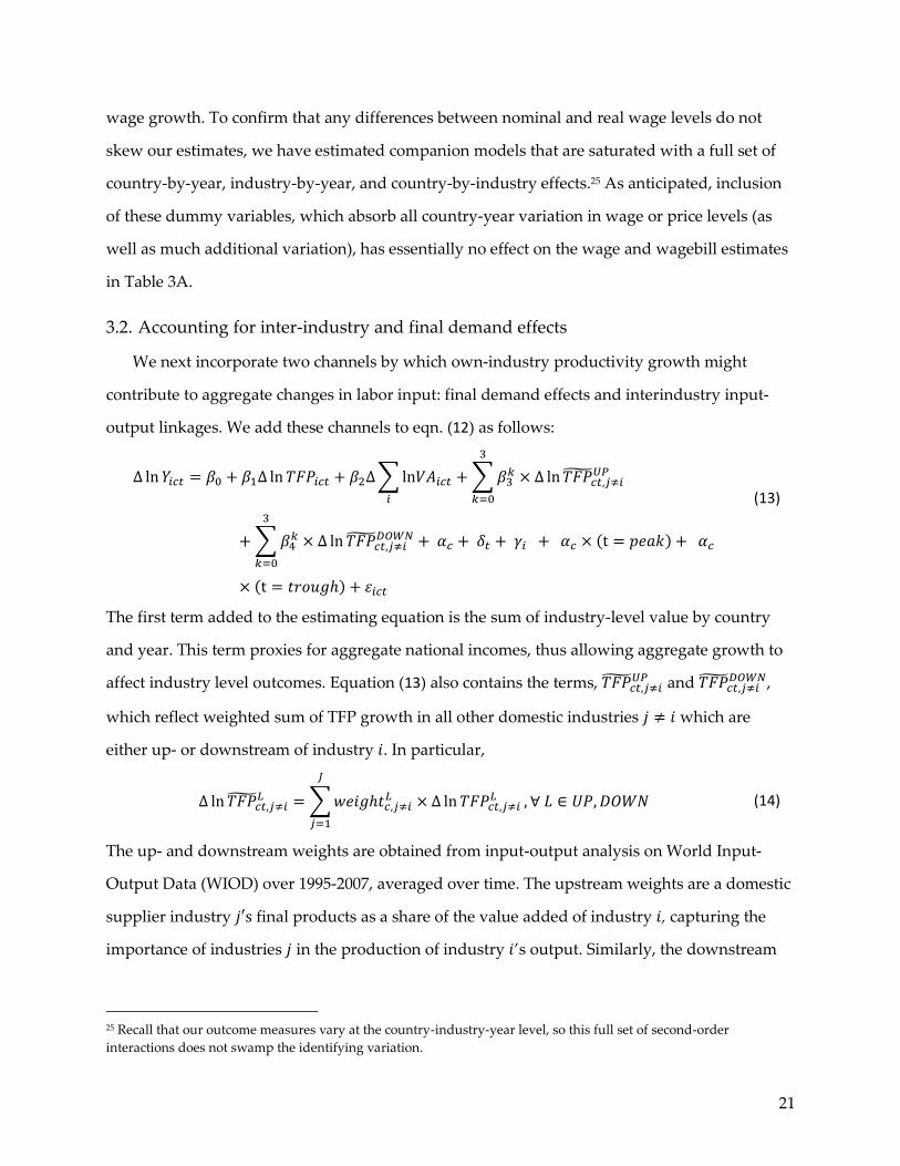
3.2. Accounting for inter-industry and final demand effects

We next incorporate two channels by which own-industry productivity growth might

contribute to aggregate changes in labor input: final demand effects and interindustry input-

output linkages. We add these channels to eqn. (12) as follows:

∆ ln𝑌𝑖𝑐𝑡 = 𝛽0 + 𝛽1∆ ln 𝑇𝐹𝑃𝑖𝑐𝑡 + 𝛽2∆∑ln𝑉𝐴𝑖𝑐𝑡𝑖

+∑𝛽3𝑘 × ∆ ln𝑇𝐹�̃�𝑐𝑡,𝑗≠𝑖

𝑈𝑃

3

𝑘=0

+∑𝛽4𝑘 × ∆ ln 𝑇𝐹�̃�𝑐𝑡,𝑗≠𝑖

𝐷𝑂𝑊𝑁

3

𝑘=0

+ 𝛼𝑐 + 𝛿𝑡 + 𝛾𝑖 + 𝛼𝑐 × (t = 𝑝𝑒𝑎𝑘) + 𝛼𝑐

× (t = 𝑡𝑟𝑜𝑢𝑔ℎ) + 휀𝑖𝑐𝑡

(13)

The first term added to the estimating equation is the sum of industry-level value by country

and year. This term proxies for aggregate national incomes, thus allowing aggregate growth to

affect industry level outcomes. Equation (13) also contains the terms, 𝑇𝐹�̃�𝑐𝑡,𝑗≠𝑖𝑈𝑃 and 𝑇𝐹�̃�𝑐𝑡,𝑗≠𝑖

𝐷𝑂𝑊𝑁,

which reflect weighted sum of TFP growth in all other domestic industries 𝑗 ≠ 𝑖 which are

either up- or downstream of industry 𝑖. In particular,

∆ ln𝑇𝐹�̃�𝑐𝑡,𝑗≠𝑖𝐿 =∑𝑤𝑒𝑖𝑔ℎ𝑡𝑐,𝑗≠𝑖

𝐿 × ∆ ln 𝑇𝐹𝑃𝑐𝑡,𝑗≠𝑖𝐿

𝐽

𝑗=1

, ∀ 𝐿 ∈ 𝑈𝑃,𝐷𝑂𝑊𝑁

(14)

The up- and downstream weights are obtained from input-output analysis on World Input-

Output Data (WIOD) over 1995-2007, averaged over time. The upstream weights are a domestic

supplier industry 𝑗′s final products as a share of the value added of industry 𝑖, capturing the

importance of industries 𝑗 in the production of industry 𝑖’s output. Similarly, the downstream

25 Recall that our outcome measures vary at the country-industry-year level, so this full set of second-order

interactions does not swamp the identifying variation.

22

weights are shares of value added of industry 𝑖 that are used in domestic industry 𝑗’s final

products, capturing the importance of industries j as end-consumers of industry i’s output.

These weights therefore account not only for shocks to an industry’s immediate domestic

suppliers or buyers but for the full set of input-output relationships among all connected

domestic industries. Formally, these weight matrices correspond to Leontief inverses of the

corresponding input-output tables. We include three annual lags in up- and downstream TFP

growth to allow for dynamics in these sectoral linkage effects.26

The third and fourth column of the four panels of Table 3A present estimates of equation

(13), which account for aggregate growth effects and inter-industry linkages. In column (3), we

estimate large effects of aggregate growth on industry-level employment (�̂�2𝐸 = 0.30), hours

(�̂�2𝐻 = 0.30), hourly wages (�̂�2

𝑊 = 0.63), and wagebills (�̂�2𝑊 = 0.93). Though these economically

sizable relationships are expected, they are nonetheless important because they underscore that

by raising aggregate value-added, industry-level productivity growth generally augments labor

demand economy-wide, even if it potentially reduces own-sector employment.

The interindustry terms, added in column (4) of each panel, indicate that productivity

growth in upstream (supplier) sectors predicts steep increases in employment, hours, and total

(nominal) wagebill (though not hourly wages) in customers sectors. Conversely, productivity

growth in downstream (customer) sectors has negligible effects on outcomes of interest in

supplier sectors. These patterns are consistent with the simple Cobb-Douglas input-output

framework in Acemoglu, Akcigit, and Kerr (2017), where innovations in a given sector generate

downstream impacts on its customer sectors, who benefit from price declines, but have no net

effect on its upstream supplier sectors because the price and quantity effects of any induced

demand shift are offsetting. These inter-industry relationships reinforce the point that an

26 We do not find empirical support for any lagged effect of own-industry TFP growth.

23

exclusive focus on own-industry effects of productivity growth on labor inputs would lead to

misleading conclusions for labor aggregates. 27

Based on the current set of findings, we can draw no strong conclusion for whether

automation (as proxied by TFP) is labor-augmenting or labor-displacing in the sectors where it

occurs. Since the net effect on wagebill is positive, it is tempting to interpret the net effect as

labor-augmenting. But this inference would be premature. In our model, a technological change

is labor-displacing if it reduces labor’s share of output. Our results so far do not reveal whether

this is occurring. To adjudicate among these competing interpretations, we harness information

on industry price levels, value-added, and payments to labor as a share of value-added. We

report estimates for these outcomes, fit with equation (13), in Table 3B. In the first panel, we

find a strong positive association between growth in industry TFP and growth in nominal

value-added. The estimated value-added-TFP elasticity is approximately equal to 0.45 in all

columns. Thus, a one percent rise in TFP predicts a half-percent rise in nominal value-added.

If this rise is indeed a consequence of rising industry productivity, as we expect, then it

should be accompanied by a fall in industry price. Panel B shows that this is indeed the case. A

one percent rise in industry TFP predicts a fall of approximately 0.40 percent in the industry

price level (that is, in the price deflator). If one is willing to make the strong assumption that

rising TFP affects industry output only through its effect on the output price, then these

estimates further imply an output demand elasticity of 1.2 (�̂� = −0.455

0.387= −1.2), which appears

prima facie reasonable.28

The final panel of Table 3B pulls together these empirical threads by estimating the

relationship between own-sector TFP growth and labor’s share of value-added, equal to

nominal wagebill over nominal value-added. As implied by the estimates in panel D of Table

27 Because the EU KLEMS data contain coarse skill measures, we cannot confidently assess to what degree rising

wage payments are driven by changing skill composition versus rising wages for given skill levels. However,

supplementary analyses performed by skill level for the three skill groups reported in EU KLEMS find that the wage-

TFP elasticity is almost identical across all three groups. Thus, despite the coarse measurement, we strongly suspect

that changing skill composition is unlikely to be the entire story.

28 Alternatively, a reduced form interpretation of these relationships is given in panel C, where we estimate that a one

percent rise in TFP predicts a rise in real output of 0.84 percent. Note that the estimated effect on real value-added is

algebraically equivalent to the difference between the TFP effect on nominal output and its effect on the price level,

all in log terms.

24

3A, where we find a wagebill-TFP elasticity of 0.11, and panel A of Table 3B ,where we find a

value-added-TFP elasticity of 0.45, a rise in own-sector TFP predicts a significant fall in labor’s

share of value-added within that sector. Specifically, the point estimate in column 4 of panel D

indicates that a one percent rise in TFP predicts a 0.34 percent fall in labor’s share of value-

added.

We emphasize that this own-industry effect does not correspond to the total implied impact

of rising TFP on the labor share since it abstracts from both the aggregate growth and input-

output channels. We quantify those channels below. For now, we note that the point estimate

for the elasticity of labor-share with respect to aggregate growth is small in magnitude

(coefficient of −0.08) and statistically insignificant, as is the estimated effect of TFP growth in

customer (downstream) industries on own-industry labor share (coefficient of 0.07, also

statistically insignificant). However, the coefficient on TFP on supplier (upstream) industries is

large and precisely estimated with a slope of 0.79. At face value, this pattern of point estimates

suggests that while own-sector productivity growth may predict a fall in own-industry labor-

share, interindustry linkages provide a countervailing effect.

Table 4 gathers the primary estimates from Tables 3A and 3B into compact form. The

models in Table 4 additionally include a set of country by industry by business-cycle indicator

variables to allow the procyclicality of TFP to differ by industry within each country according

to the state of the business cycle. A comparison of the Table 4 estimates with their counterparts

in Tables 3A and 3B indicates that these further cyclicality controls have essentially no effect on

the point estimates.

3.3. Using Low-Frequency Variation

Before assessing the economic magnitude of these relationships in Section 4, we address a

natural concern with our estimates, which is that they rely on high-frequency (annual) variation

for identification. Although we include a large set of fixed effects and time lags—including

country-by-industry specific business cycle effects—to purge cyclical components of TFP and

short-run adjustment dynamics, it is important to verify that our main results hold when using

low frequency variation. This is done in Table 5 by fitting long differences of equation (13) on

25

non-overlapping time intervals. Panel A of the table estimates the model with annualized 5-year

changes, while panel B employs annualized 10-year changes. Both panels include country,

industry, period, as well as country-by-industry and industry-by-period fixed effects.29

Results are robust to this modification in model specification. As before, industries

experiencing relatively rapid TFP growth see a decline in employment and hours worked, a

modest rise in wagebill, and a substantial increase in value-added. Estimated final demand

relationships are of the same sign and comparable magnitude to earlier estimates. Interindustry

linkages generally show somewhat smaller effects: upstream impacts on hours and wagebill are

less positive and downstream impacts are more negative.

Of greatest interest, we continue to estimate a negative and highly significant relationship

between TFP increase and labor-share declines at the industry level. The point estimates

obtained using lower frequency are smaller than in the high-frequency models: −0.26 using 5-

year changes and −0.16 using 10-year changes, as compared to −0.34 when using annual

changes. Note, however, that the countervailing effects of upstream spillovers on labor share

are less positive in these lower-frequency models. As a consequence, the implied net effects are

similar to those obtained using annual variation. All told, these low-frequency models imply a

predicted labor share decline of 3.4 to 6.3 log points due to TFP growth over the 1970-2007

period. These predictions bracket the corresponding predicted effect of 5.3 log points obtained

when using annual variation.30

Lastly, Appendix Table 3A estimate our main specification (Tables 4) while filtering the

main explanatory variables (TFP, aggregate value-added) using a three-year backward-looking

moving average process so as to smooth out any remaining short-run fluctuations. Our

conclusions are unaltered by this modification.

29 A small number of intervals is shorter than this 5- or 10-year length, as countries sometimes enter or exit the dataset

mid-interval (see Table 1A). In particular, for panel A, 81% of periods are exactly 5 years in length. The minimum

period length we use is 2 years, and the maximum is 7 years (to cover 2000-2007). For panel B, 60% of periods are 10

years in length, 20% are 7 years in length (to cover 2000-2007), and the minimum period length is again 2 years.

30 Details on these calculations are given in the next session.

26

4. Quantitative implications

Our primary estimating equation (eqn. 13) permits industry-level productivity growth to

affect outcomes of interest through three channels: own-industry effects, cross-industry input-

output linkages, and final demand effects. This three-level structure means that the net effect of

an increment to TFP occurring in any given sector on the aggregate outcome of interest is not

directly readable from the table.

To quantify the operation of all three channels simultaneously, we differentiate equation

(13) with respect to 𝑇𝐹𝑃 in some industry 𝑖 to obtain:

𝜕 ln𝑌𝑐𝑡𝜕 ln𝑇𝐹𝑃𝑖𝑐𝑡

= 𝛾𝑖𝑐�̂�1 + �̂�2�̂�𝑉𝐴∑𝛾𝑖𝑐

𝑖

+∑(𝛾𝑗𝑐∑�̂�3𝑘 ×𝑤𝑒𝑖𝑔ℎ𝑡𝑐,𝑗≠𝑖

𝑈𝑃

3

𝑘=0

)

𝑗≠𝑖

+∑(𝛾𝑗𝑐∑�̂�4𝑘 × 𝑤𝑒𝑖𝑔ℎ𝑡𝑐,𝑗≠𝑖

𝐷𝑂𝑊𝑁

3

𝑘=0

)

𝑗≠𝑖

,

(15)

where 𝑌𝑐𝑡 is an outcome of interest such as country-level employment in year 𝑡, and the scalar

𝛾𝑖𝑐 equals industry 𝑖′𝑠 share in country 𝑐′𝑠 value-added. The first term in this expression is the

direct (own-industry) effect of TFP growth in industry 𝑖 on own-industry employment,

weighted by industry 𝑖′𝑠 share in country 𝑐′𝑠 value added (𝛾𝑖𝑐). The second term is the final

demand effect, equal to the elasticity of employment with respect to aggregate value-added (�̂�)

multiplied by the derivative of aggregate value added with respect to industry 𝑖′𝑠 value-added

(also equal 𝛾𝑖𝑐) further scaled by the estimated elasticity of industry-value added with respect to

𝑇𝐹𝑃 from column 6 of Table 4, which we write as �̂�𝑉𝐴 in this expression. The third and fourth

terms are the contributions of upstream and downstream linkages. These are equal to the

relevant Leontief inverse weight of industry 𝑖′𝑠 TFP on upstream or downstream industries,

multiplied by the estimated input-output effects in column 1 of Table 4, finally multiplied by

each upstream or downstream industry’s share in aggregate value-added.

Figures 1A, 1B, and 1C report the results of this calculation for overall employment, for

hours of labor input, and for labor share respectively.31 The first bar in Figures 1A corresponds

to the direct-effect of TFP growth on own-industry employment. Its height of −0.068 implies

31 Bootstrap confidence intervals are based on 100 replications.

27

that on average, productivity growth reduced own-industry employment by approximately 2.5

percent over the full 37-year period (0.068/100 × 37 = 2.5). The second bar (“final demand”)

with height 0.073 indicates that the countervailing indirect effect of rising aggregate value-

added on employment more than offset this direct effect. The third bar (“upstream effect”)

indicates an additional, large positive effect of rising productivity in upstream (supplier)

industries on employment in customer industries. The fourth bar (“downstream effect”)

indicates a negligible employment reduction in downstream (supplier) industries. The final bar

(“net effect”) sums over these four components to estimate a net positive effect of productivity

gains on aggregate employment, totally approximately six log points (0.16/100 × 37 = 5.92)

over the outcome period.

When we perform the same exercise for hours rather than workers in Figures 1B, we reach a

comparable conclusion: the negative effects of rising productivity on own-industry employment

and hours are more than offset by induced effects on aggregate demand and by employment

growth in customer sectors.

The analogous exercise for labor share in Figure 1C, however, yields a different result. The

direct effect of rising TFP on own-industry labor shares of −0.23/100 log points annually are

partly offset by induced labor share gains in customer industries, equaling 0.12/100 log points

annually. Meanwhile, there is no offset through either final demand or impacts in supplier

industries. This yields a net effect of −5.3 log points over the entire 1970-2007 period

(−0.143/100 × 37 = −0.053), which is similar to the observed change of −0.169/100 log points

annually (see Table 2), or 6.3 log points cumulatively over the 37-year period.

To provide a reality check on our estimates, Figure 1D plots the net labor share predictions from

our model (on the horizontal axis) against actual observed changes by industry (on the vertical

axis). Each data point in this figure represents an industry, and the 45-degree line is added to

gauge fit. Overall, this figure shows that the estimated relationship between rising productivity

and falling labor share can explain a significant portion of the variation in actual labor share

evolution by industry. The R-squared of a value-added weighted regression is 0.25, with a

highly statistically coefficient of 0.431.

28

4.1. Exploring heterogeneity: Detailed estimates by sector

Our estimates so far restrict the impacts of productivity growth to be constant across

industries, no matter in which industry this productivity growth originates. This may be too

restrictive. Different sectors may use technologies which are differently labor-augmenting or

replacing—say, robotic assembly in manufacturing versus proliferating treatment regimens in

health services—resulting in different impacts of TFP growth on industry employment and

wages. Additionally, some sectors may face more elastic demand for their outputs—for

example because of lower demand saturation (cf. Bessen 2017)—or face higher product market

competition, resulting in stronger responses of prices and output to TFP growth.

We explore sectoral heterogeneity in the effects of TFP growth in Table 6A by relaxing the

symmetry restrictions imposed by our estimates in Table 4. Specifically, we augment equation

(13) to allow outcome-productivity elasticities and final demand effects to differ across five

broad sectors: (1) mining, utilities and construction; (2) manufacturing; (3) education and health

services; (4) capital-intensive (‘high tech’) services; and (5) labor-intensive (‘low tech’) services

(as was done earlier in Table 1B).32 The specifications in Table 6A are otherwise identical to

those in Table 4 save for these sectoral interactions.

A key take-away from this analysis is that all sectoral coefficients have the same sign across

each sectors for each outcome and most are statistically significant. This means that our earlier

findings are not driven by disparate patterns in a subset of industries. Rather, TFP growth

predicts a fall in hours, a rise in wagebill, and a fall in labor share in all sectors in which it

occurs. The estimated labor share elasticity to TFP growth is most negative (−0.37) in

manufacturing and low-tech services and is least (−0.13) in education and health sectors. The

second set of rows in the table report the final demand effects on outcomes, which are again

allowed to vary by sector. Though most sectoral coefficients are comparable, we find that rising

32 Specifically: Mining, utilities, and construction corresponds to industries C, E and F; Manufacturing is industries 15

through 37; Education and health services are industries M and N; High-tech services are industries 64, J, and 71 to

74; and Low-tech services are industries 50 to 52, H, 60 to 63, 70, and O. This particular high- and low-tech services

division is obtained from the OECD.

29

aggregate income predicts a fall in labor share in the mining and utilities sector, though not in

other sectors.33

4.2. Exploring heterogeneity: Detailed estimates by decade

Table 6B explores how these relationships evolve over time. To the extent that technologies

have become more labor-displacing—as popular accounts suggest—we would expect the

employment and labor share effects of TFP growth to turn more negative over time. The

estimates in this table indeed support such a story: the labor share elasticity to TFP growth

becomes successively more negative across the four decades in our sample, from −0.14 in the

1970s to −0.32 in the 1980s to −0.34 in the 1990s to −0.47 in 2000s.34 Turning to the various

components of the labor share, it can be seen that this is mostly coming from a monotonically

declining wagebill-TFP elasticity (from 0.17 in the 1970s to 0.04 in the 2000s) coupled with a

nearly constant real output response. As a result, TFP growth predicts an increasingly large

drop in own-industry labor-share in successive decades.35

These own-industry effects ignore the influence of final demand and inter-industry linkages,

however. To assess their contributions, Figures 2A and 2B report the predicted effect of TFP on

labor hours and labor share, respectively, operating through each channel—own-industry, final

demand, and inter-industry linkages—during each of the four decades of the sample. Figure 2A

indicates that the estimated impact of rising TFP on total labor hours was positive in each

decade, with the largest predicted effect in the 1980s and the smallest effects in the 1970s and

2000s. Most of this cross-decade variation in magnitudes stems from differences in the growth

rate of TFP, which was slowest in the 1970s and 2000s and most rapid in the 1980s and, to a

lesser extent, the 1990s.

33 Appendix Table 3B presents corresponding estimates using filtered TFP and aggregate income measures to purge

high frequency variation in TFP. These estimates are largely comparable to the estimates using higher frequency

variation in Table 6A.

34 This result also holds when considering a (more) balanced panel of countries where each country contributes at

least one observation of in each of the four decades.

35 Appendix Table 3C presents corresponding estimates using filtered TFP and aggregate income measures to purge

high frequency variation in TFP. These estimates are largely comparable to the estimates using higher frequency

variation in Table 6B.

30

Figure 2B reports a far starker pattern for the contribution of rising productivity to the

evolution of labor shares. This effect is essentially zero in the 1970s and then is consistently

negative in each of three following decades, with an estimated net impact of −4.51 log points

between 1980 and 2007. It is natural to ask how much of this decadal variation stems from

differences in the growth rate of TFP across periods versus decadal differences in the predictive

relationship between TFP and the various components of labor share adjustment. Figure 2C

answers this question by calculating a counterfactual in which TFP growth is counterfactually

equalized across all time periods at the mean overall growth rate of TFP for 1970 – 2007.

Strikingly, this figure shows that the predicted effect of a given increment to TFP is successively

more negative for aggregate labor-share in each decade of the sample; thus, the change in

coefficients across periods plays a first order role. This time pattern stems in turn from a

decade-over-decade steepening of the relationship between TFP growth and own-industry

labor share decline. The final demand effect of rising TFP on labor share is essentially zero in

the 1970s and 1980s, becomes slightly negative in the 1990s, and turns strongly negative in the

2000s.36 The fact that both own-industry and final demand effects become increasingly (and

monotonically) more negative across each decade is potentially consistent with a scenario

where technological progress has become secularly more labor-displacing.

To provide a sense of how successfully these models capture the relevant variation in the

data, Figure 2D presents a scatter plot of predicted versus observed changes in industry-level

labor shares in each decade, where each decade’s data points are plotted with a distinct marker

to highlight cross-decade differences. The 1970s stand out as the decade where there is little

change observed in industry-level labor shares. Our model predicts comparatively little change

in this decade as well. The subsequent three decades reveal far larger falls in industry labor

shares and far more variation across industries in magnitudes. The correspondence between the

model fits and observed changes in considerably closer in these three decades.

36 We do not allow the inter-industry slopes to vary by decade because these estimates become highly imprecise when

we add parameters. The data do not reject the null hypothesis that this upstream and downstream effects are

constant across decades.

31

These by-decade estimates only cover outcomes through 2007, when the coverage of our

primary EUKLEMS database ceases. Fortunately, a 2017 EUKLEMS database release (Jäger and

Van Ark 2017) can be used to cover the intervening years up to 2015, albeit for a smaller subset

of countries (13 in total, see Appendix Table 1A for coverage). Although these data are not

directly comparable to the earlier release because of changes in both the industry classification

(see Appendix Table 1B) and in data construction, we use them to check the qualitative

robustness of our direct and final demand effects for the post-2007 period.

Table 7 reports estimates of equation (12) for 2007 - 2015, including the same full set of fixed

effects used in Table 4.37 Result are very similar for the most recent decade in the long

EUKELMS panel. Industry-level TFP growth is associated with a substantial rise in nominal

value-added, a (small) decline in hours worked, and no increase in the wagebill, all of which are

consistent with the pattern prevailing in 2000-2007 (see Table 6B). Also, as in earlier decades,

there is a strongly positive elasticity of hours, wagebill, and value-added with final demand, as

well as a zero elasticity of labor-share with respect to final demand. A rise in TFP predicts an

even larger decline in own-industry labor share in the post-2007 period than earlier in the

decade (−0.64 versus −0.47). Although not reported in Table 7, these patterns are unaffected by

including a less stringent set of fixed effects or by excluding the Great Recession years.

Although we hesitate to draw strong inferences given the many differences—including country

coverage, industry classification, and measurement constructs—between the pre- and post-2007

EUKLEMS databases, the Table 7 estimates do not suggest that the increasingly negative

relationship between productivity growth and own-industry labor-share seen in Table 6B,

particularly in the final decade of the sample, reverses course after 2007.

5. Is automation labor-displacing? Applying direct measures of

innovation and automation

We have so far used TFP growth as an omnibus measure of automation. This has the

advantage of not restricting the analysis to a specific type of technology and its associated

37 We do not estimate the interindustry linkage terms for this short time interval since this would require inclusion of

three lag terms, truncating our event window by three of eight years.

32

measurement issues. But TFP is ultimately a residual, so it is difficult to know what it

corresponds to. Moreover, one may be concerned that TFP growth is endogenous to, or

simultaneously determined with, some of the outcomes we consider, even net of the fixed

effects included in the specifications.

To address these concerns, we consider two direct industry-level measures of automation

and technological change: patenting flows (as in Acemoglu, Akcigit, and Kerr 2017), and

adoption of industrial robotics (as in Graetz and Michaels 2015, and Acemoglu and Restrepo

2017, among others). We use these automation measures as instrumental variables for industry-

level TFP growth to isolate variation in productivity growth that is both directly related to

technological advances and plausibly exogenous. As shown below, both measures of

technological change are significant predictors of industry-level productivity growth. One may

of course question the plausibility of the implicit exclusion restriction implied by these 2SLS

estimates, i.e., that patent flows and robot penetration exert a causal effect on outcomes of

interest exclusively through their impact on TFP. Whether one accepts this restriction or simply

views these measures as proxies for industry-level technological progress, the rescaling of each

measures in terms of units of TFP—as is implicitly done by the first stage of the 2SLS

estimates—facilitates interpretation.

We construct patent citations by year for patents granted to both US and non-US inventors

using US Patent and Trademark Office (USPTO) data by US SIC industry, cross-walked to the

EUKLEMS industry level. These data are sourced from Autor et al. (2017a), who match patent

grants to their respective corporate owners and then to industry codes based on corporate

owners’ industry affiliations. Appendix Table 4 reports the mean log number of patent citations

by industry and by inventor nationality (U.S. versus non-U.S.). This table highlights the

substantial heterogeneity in patent flows across sectors, with the highest levels of patenting

occurring in chemicals as well as electrical equipment. We consider this patenting activity as an

input in the innovation and automation process at the industry level.

Table 8 reports estimates of our baseline results using log patent citations as an

instrumental variable for TFP growth. To reduce the possibility of simultaneity, we use patent

citations for non-US inventors to instrument TFP growth in the US and use patent citations for

33

US inventors to instrument TFP growth outside the US. (In point of fact, our results are quite

similar when using total patent citations for both.) All specifications control for growth in

nominal value added by country-year and include country and year fixed effects, as well as

country-specific business cycle effects.

The first stage, reported in the lower panel of the table, is highly significant: citations to

patents originating in an industry are strong predictors of TFP growth within that industry.

Notably, the second stage results are qualitatively similar to our OLS estimates: instrumented

TFP growth has a statistically significant negative effect on hours worked and on labor share,

consistent with our baseline findings. The point estimate for the impact of productivity

growth—here instrumented by foreign country patent citation flows—equal to −0.35 is highly

comparable to the corresponding OLS estimate in Table 4 (column 8), though of course the

standard error of the 2SLS estimate is much larger.38

As a second instrumental variables strategy, we use the introduction of robotics as a

concrete example of a recent innovation engendering a wave of automation. We rely on

International Federation of Robotics (IFR) data on robot purchases by country-industry-year,

and we follow Acemoglu and Restrepo’s (2017) industry classification scheme to match these

data to KLEMS, though we slightly modify their scheme to account for the higher aggregation

of our TFP data across industries. These data cover 16 more aggregate industries over 1993 to

2007 for all but four countries in our sample.39 Appendix Table 5 provides an overview of this

classification as well as summary statistics on the number of robots per 1,000 workers and the

average annual change therein, reflecting automation at the industry level. These summary

statistics show that transport equipment is by far the most robot-intensive industry, followed by

plastics and chemicals, metals, and electronics. These are also the sectors where robot

penetration is rising most rapidly—logically, since robots were quite scarce until recently—

though it rises in most industries.

38 We do not consider input-output linkages in our instrumental variables estimates since we lack statistical power to

identify these second-order terms in 2SLS models.

39 Not included in IFR data are Canada, Ireland, and Luxembourg. Japan is excluded because of unreliable data, see

Acemoglu and Restrepo (2017).

34

Table 9 reports estimation results from instrumenting TFP growth by the annual change in

the number of robots per 1,000 workers, controlling for a country and year fixed effects as well

as country-specific business cycle effects. As with patenting, robot penetration is a significant

predictor of industry TFP. The first stage estimate suggests that the addition of one robot per

1,000 workers increases TFP by a statistically significant 0.175 log points. Second stage results

are less precisely estimated, likely due to the relatively small number of observations, but are

qualitatively similar to our OLS results. We estimate negative direct effects of automation—that

is, TFP growth instrumented by robot adoption—on both hours worked and on the labor share.

In the case of hours worked, we estimate that final demand effects serve to counterbalance the

negative direct effect of automation on hours. But, as in our previous results, no such

compensating effect is found for the labor share. The point estimate for the impact of

automation on own-industry labor share is −0.195. While too imprecise to draw any confident

statistical statement, this point estimate is certainly in the ballpark of our main estimates.

Overall, these results using direct measures of automation appear supportive of our prior

findings on TFP growth more broadly.

6. Concluding remarks

Although our motivating model of labor displacement envisages a setting where tasks are

reallocated from labor to capital in an aggregate production function, this high-level

representation is consistent with a variety of within- and between- firm adjustments. At one

extreme, every firm in an industry undergoing technological progress might substitute capital

for labor in a subset of tasks. Alternatively, absent any within-firm change in task allocation, a

technological advance might spur an increase in industry market share among relatively

capital-intensive firms and a concomitant decline among relatively labor-intensive firms.40

Under either scenario, labor’s share in industry value-added would fall. Our analysis cannot

speak to these within- versus between-firm dynamics. Nevertheless, we believe that the scope

40 The relevance of this latter mechanism is supported by the industry-by-establishment analysis of changes in

industry labor shares reported in Autor et al. (2017b).

35

of the evidence presented here complements more granular, but narrower firm and

establishment-level studies.

7. References

Abramovitz, Moses. 1956. “Resource and Output Trends in the U.S. since 1870.”American

Economic Review Papers and Proceedings, 46(2), 5-23.

Acemoglu, Daron, David Autor, David Dorn, Gordon Hanson, and Brendan Price. 2016.

“Import Competition and the Great U.S. Employment Sag of the 2000s.” Journal of Labor

Economics, 34, S1 (Part 2), S141–S198

Acemoglu, Daron, Ufuk Akcigit, and William Kerr. 2017. “Networks and the Macroeconomy:

An Empirical Exploration.” In Martin Eichenbaum and Jonathan A. Parker (eds.), NBER

Macroeconomics Annual, 31, Chicago: University of Chicago Press.

Acemoglu, Daron, and David Autor. 2011. “Skills, Tasks and Technologies: Implications for

Employment and Earnings.” in O. Ashenfelter and D. Card, eds., The Handbook of Labor

Economics Volume IV, Amsterdam: Elsevier.

Acemoglu, Daron, and Veronica Guerrieri. 2008. “Capital Deepening and Nonbalanced

Economic Growth.” Journal of Political Economy 116 (3): 467–98.

Acemoglu, Daron and Pascual Restrepo. 2017. “Robots and Jobs: Evidence from U.S. Labor

Markets.” NBER Working Paper No. 23285, March.

Acemoglu, Daron and Pascual Restrepo. 2018a. “Artificial Intelligence, Automation and Work.”

NBER Working Paper No. 24196, January.

Acemoglu, Daron and Pascual Restrepo. 2018b. “The Race Between Machine and Man:

Implications of Technology for Growth, Factor Shares and Employment.” American Economic

Review, forthcoming.

Akerman, Anders, Ingvil Gaarder, and Magne Mogstad. 2015. “The Skill Complementarity of

Broadband Internet.” Quarterly Journal of Economics 130(4): 1781–1824.

Alexopoulos, Michelle, and Jon Cohen. 2016. “The Medium Is the Measure: Technical Change

and Employment, 1909–1949.” Review of Economics and Statistics 98(4): 792–810.

Autor, David. 2015. “Why Are There Still So Many Jobs? The History and Future of Workplace

Automation.” Journal of Economic Perspectives 29(3), 3 – 30.

Autor, David, David Dorn, Gordon H. Hanson, Gary Pisano, and Pian Shu. 2017a. “Foreign

Competition and Domestic Innovation: Evidence from U.S. Patents.” MIT Working Paper,

December.

36

Autor, David, David Dorn, Lawrence F. Katz, Christina Patterson, and John Van Reenen. 2017b.

“The Fall of the Labor Share and the Rise of Superstar Firms.” NBER Working Paper No.

23396, May.

Autor, David H., Lawrence F. Katz, and Melissa S. Kearney. 2008. “Trends in US Wage

Inequality: Revising the Revisionists.” Review of Economics and Statistics 90(2): 300-323.

Autor, David H., Frank Levy, and Richard J. Murnane. 2003. “The Skill Content of Recent

Technological Change: An Empirical Exploration.” Quarterly Journal of Economics 118(4):

1279–1333.

Autor, David H. and Anna M. Salomons. 2017. “Robocalypse Now—Does Productivity Growth

Threaten Employment?” European Central Bank Sintra Forum conference paper, June 2017.

Autor, David, and Melanie Wasserman. 2013. Wayward Sons: The Emerging Gender Gap in

Education and Labor Markets. Washington, DC.

Barkai, Simcha. 2016. “Declining Labor and Capital Shares.” Working Paper, University of

Chicago.

Basu, Susanto, and John Fernald. 2001. “Why is Productivity Procyclical? Why Do We Care?” In

Charles R. Hulten, Edwin R. Dean and Michael J. Harper, eds., New Developments in

Productivity Analysis, Chicago: Univ of Chicago Press, 225–302.

Baumol, William J. 1967. “Macroeconomics of Unbalanced Growth: The Anatomy of Urban

Crisis.” American Economic Review 57(3): 415–26.

Berg, Andrew, Edward F. Buffie, and Luis-Felipe Zanna. 2017. “Robots, Growth, and Inequality:

Should We Fear the Robot Revolution? (The Correct Answer is Yes).” IMF Working Paper

WP/17/XX, February.

Bessen, James. 2017. “Automation and Jobs: When Technology Boosts Employment.” Boston

University School of Law: Law & Economics Paper No. 17-09, April.

Blundell, Richard. 2016. “Labour Markets and Inclusive Growth” Presentation to the U.K.

Growth Commission, Nov. 17.

Brynjolfsson, Erik, and Andrew McAfee. 2014. The Second Machine Age: Work, Progress, and

Prosperity in a Time of Brilliant Technologies. New York and London: W.W. Norton &

Company.

Dao, Mai, Mitali Das, Zsoka Koczan, and Weicheng Lian. 2017. “Why is Labor Receiving a

Smaller Share of Global Income? Theory and Empirical Evidence,” IMF Working Paper.

Elsby, Mike, Bart Hobijn, and Aysegul Sahin. 2013. “The Decline of the U.S. Labor Share.”

Brookings Papers on Economic Activity, 1-42.

37

Dustmann, Christian, Bernd Fitzenberger, Uta Schönberg, and Alexandra Spitz-Oener. 2014.

“From Sick Man of Europe to Economic Superstar: Germany’s Resurgent Economy.” Journal

of Economic Perspectives 28(1): 167–188.

Ford, Martin. 2015. Rise of the Robots: Technology and the Threat of a Jobless Future. New York: Basic

Books.

Frey, Carl Benedikt, and Michael A. Osborne. 2015. “The Future of Employment: How

Susceptible are Jobs to Computerisation?” Technological Forecasting and Social Change 114:

254–280.

Goos, Maarten, Alan Manning, and Anna Salomons. 2009. “Job Polarization in Europe.”

American Economic Review Papers and Proceedings 99(2): 58-63.

Goos, Maarten, Alan Manning, and Anna Salomons. 2014. “Explaining Job Polarization:

Routine-Biased Technological Change and Offshoring.” American Economic Review 104(8):

2509–26.

Goos, Maarten, Emile Rademakers, Anna Salomons, and Marieke Vandeweyer. 2015.

“Routinization, Between-Sector Job Polarization, Deindustrialization and Baumol’s Cost

Disease.” Utrecht School of Economics Working Paper 15-15, December.

Graetz, Georg, and Guy Michaels. 2015. “Robots at work.” CEP Discussion No. 1335.

Gregory, Terry, Anna Salomons, and Ulrich Zierahn. 2016. “Racing With or Against the

Machine? Evidence from Europe.” Utrecht School of Economics, Tjalling C. Koopmans

Research Institute, Discussion Paper Series 16-05, July.

Herald Press, The. 1966. “Skirting the Automation Question.” February 7, p. 2. (The Herald Press

of St. Joseph, Michigan.)

Hogan, Andrew and Brian Roberts. 2015. “Occupational Employment Projections to 2024.”

Monthly Labor Review, U.S. Bureau of Labor Statistics, 2015.

Johnston, Louis. 2001. “The Growth of the Service Sector in Historical Perspective: Explaining

Trends in U.S. Sectoral Output and Employment, 1840-1990.” St. John’s University Working

Paper.

Jones, Charles I, and Paul Romer. 2010. “The New Kaldor Facts: Ideas, Institutions, Population,

and Human Capital.” American Economic Journal: Macroeconomics 2: 224–45.

Kaldor, Nicholas. 1961. “Capital Accumulation and Economic Growth.” in The Theory of Capital,

ed. F. A. Lutz and D. C. Hague, 177–222. New York: St. Martins Press.

Karabarbounis, Loukas and Brent Neiman. 2014. “The Global Decline of the Labor Share.”

Quarterly Journal of Economics, 129(1), 61-103.

38

Katz, Lawrence, and David Autor. 1999. “Changes in the Wage Structure and Earnings

Inequality.” in O. Ashenfelter and D. Card, eds., The Handbook of Labor Economics Volume III,

Amsterdam: Elsevier.

Keynes, John Maynard, 1939. “Relative Movements of Real Wages and Output.” Economic

Journal 49, 34-51

Leontief, Wassily. 1983. “National Perspective: The Definition of Problem and Opportunity,” in

National Academies, The Long-term Impact of Technology on Employment and Unemployment: A

National Academy of Engineering Symposium, June 30, p3.

Matsuyama, Kiminori. 2002. “The Rise of Mass Consumption Societies.” Journal of Political

Economy 110(5): 1035–1070.

Michaels, Guy, Ashwini Natraj, and John Van Reenen. 2013. “Has ICT Polarized Skill Demand?

Evidence from Eleven Countries over Twenty-Five Years.” Review of Economics and Statistics

96 (1): 60–77.

Moulton, Brent R. 1986. “Random Group Effects and the Precision of Regression Estimates.”

Journal of Econometrics 32(3): 385-397.

Montiel Olea, José Luis, and Carolin Pflueger. 2013. “A Robust Test for Weak Instruments.”

Journal of Business & Economic Statistics 31 (3): 358-369.

New York Times, The. 1927. “Davis Says Labor Needs New Outlet.” September 5.

Ngai, L. Rachel, and Christopher A. Pissarides. 2007. “Structural Change in a Multisector Model

of Growth.” American Economic Review 97(1): 429-443.

Ngai, L, and C Pissarides. 2008. “Trends in Hours and Economic Growth.” Review of Economic

Dynamics 11 (2): 239–256.

Nordhaus, William D. 2015. “Are We Approaching an Economic Singularity? Information

Technology and the Future of Economic Growth.” NBER Working Paper No. 21547,

September.

O’Mahony, Mary and Marcel Timmer. 2009. “Output, Input and Productivity Measures at the

Industry Level: the EU KLEMS Database,” Economic Journal 119(538), F374-503.

Pierce, Justin R., and Peter K. Schott. 2016. “The Surprisingly Swift Decline of US

Manufacturing Employment.” American Economic Review 106(7), 1632–1662.

Piketty, Thomas. 2014. Capital in the Twenty-First Century. Harvard University Press.

Rognlie, Matthew. 2015. “Deciphering the Fall and Rise in the Net Capital Share: Accumulation

or Scarcity?” Brookings Papers on Economic Activity, 1-69.

39

Sachs, Jeffrey D., and Laurence J. Kotlikoff. 2012. “Smart Machines and Long-Term Misery.”

NBER Working Paper 18629, December.

Sanderson, Eleanor, and Frank Windmeijer. 2016. “A Weak Instrument F-test in Linear IV

Models with Multiple Endogenous Variables.” Journal of Econometrics 190(2): 212–221.

Solow, Robert M. 1956. “A Contribution to the Theory of Economic Growth.” Quarterly Journal

of Economics 70 (1): 65–94.

Stansbury, Anna and Lawrence H. Summers. 2017. “Productivity and Pay: Is the Link Broken?”

NBER Working Paper No. 24165, December.

Susskind, Daniel. 2017. “A Model of Technological Unemployment.” Oxford University

Working Paper, April.

Timmer, Marcel P., Erik Dietzenbacher, Bart Los, Robert Stehrer, and Gaaitzen J. de Vries. 2015.

“An Illustrated User Guide to the World Input–Output Database: The Case of Global

Automotive Production,” Review of International Economics 23: 575–605.

Van Ark, Bart, and Kirsten Jäger (2017). “Recent Trends in Europe's Output and Productivity

Growth Performance at the Sector Level, 2002-2015“, International Productivity Monitor 33,

Fall 2017.

Zeira, Joseph. 1998. “Workers, Machines, and Economic Growth,” Quarterly Journal of Economics,

113(4): 1091–1117.

40

8. Model Appendix

The derivations in this Appendix are directly reproduced from Acemoglu and Restrepo (2018b)

with minor changes to accommodate the modifications made to the model for our exposition.41

Factor demands are derived as follows. Suppose that Assumption A1 holds. Denote by 𝑝(𝑥)

the price of task 𝑥. Using Assumption A1, this price is

𝑝(𝑥) =

{

𝑅

𝛼𝑀𝛾𝑀(𝑥) if 𝑥 ∈ [𝑁 − 1, 𝐼]

𝑊

𝛼𝐿(𝑥)𝛾𝐿if 𝑥 ∈ [𝐼, 𝑁] .

(16)

Due to the Cobb-Douglas structure of (1), the expenditure on task 𝑥 is equal to 𝑦(𝑥)𝑝(𝑥) for

all 𝑥 and hence the output of task 𝑥 is

𝑦(𝑥) =𝑌

𝑝(𝑥). (17)

Demands for machinery and labor, respectively, in task 𝑥 are

𝓂(𝑥) = {

𝑌

𝑅 if 𝑥 ∈ [𝑁 − 1, 𝐼]

0 if 𝑥 ∈ [𝐼, 𝑁]

(18)

and

ℓ(𝑥) = {0 if 𝑥 ∈ [𝑁 − 1, 𝐼]𝑌

𝑊if 𝑥 ∈ [𝐼, 𝑁]

(19)

Since labor and machinery are both inelastically supplied, we can sum the demands for each

factor and set it equal to supply to obtain market clearing conditions:

𝑀 =𝑌

𝑅(𝐼 − 𝑁 + 1) (20)

and

𝐿 =𝑌

𝑊(𝑁 − 𝐼). (21)

Equations (20) and (21) can be inverted to obtain expressions for the equilibrium rental and

wage rates 𝑅 and 𝑊: 𝑅 = (𝑌 𝑀⁄ )(𝐼 − 𝑁 + 1) and 𝑊 = (𝑌 𝐿⁄ )(𝑁 − 𝐼).

To derive the expression for aggregate output, we use the price of the final good 𝑌 as the

numeraire. With the final good price constant at unity, we have

41 These modifications are limited to adding the two factor-augmenting terms 𝛼𝐾 and 𝛼𝐿 to the model.

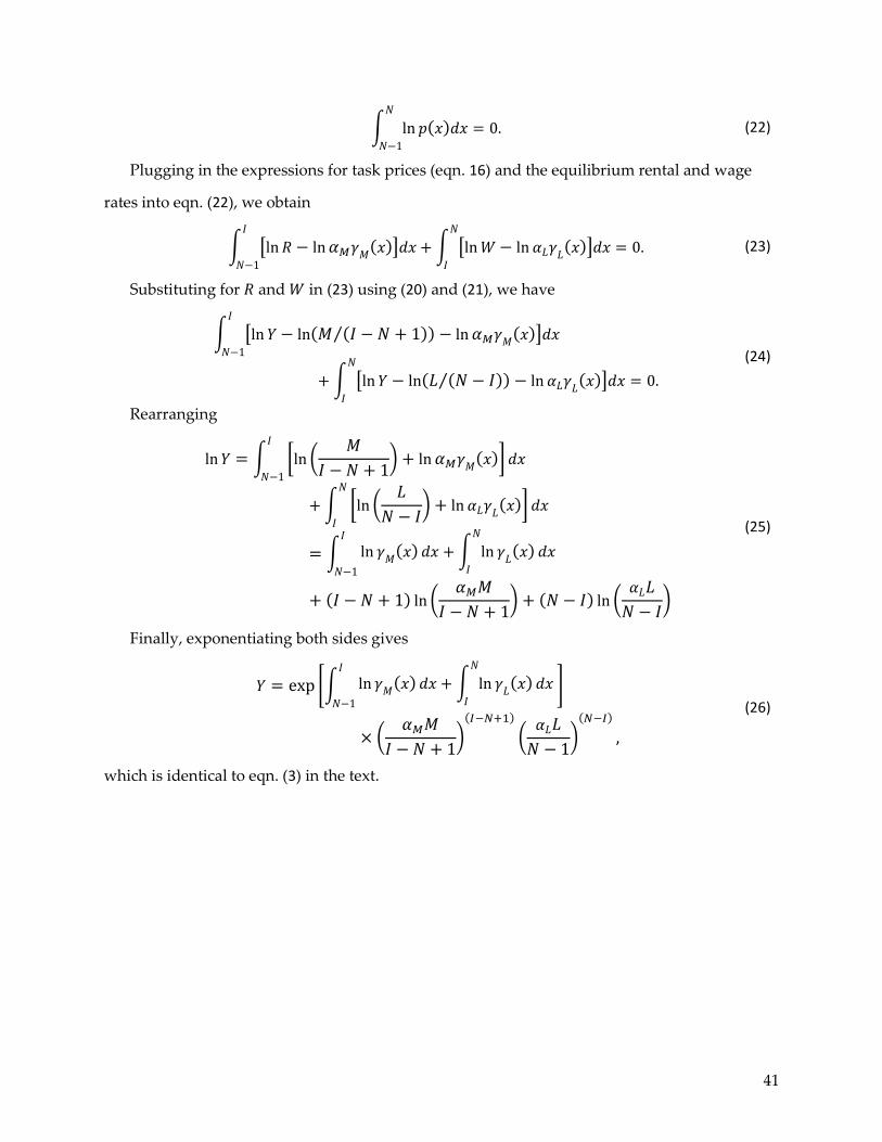
41

∫ ln 𝑝(𝑥)𝑑𝑥 = 0. 𝑁

𝑁−1

(22)

Plugging in the expressions for task prices (eqn. 16) and the equilibrium rental and wage

rates into eqn. (22), we obtain

∫ [ln 𝑅 − ln𝛼𝑀𝛾𝑀(𝑥)]𝑑𝑥 +∫ [ln𝑊− ln 𝛼𝐿𝛾𝐿(𝑥)]𝑑𝑥 = 0.𝑁

𝐼

𝐼

𝑁−1

(23)

Substituting for 𝑅 and 𝑊 in (23) using (20) and (21), we have

∫ [ln 𝑌− ln(𝑀 (𝐼 − 𝑁 + 1)⁄ ) − ln𝛼𝑀𝛾𝑀(𝑥)]𝑑𝑥𝐼

𝑁−1

+∫ [ln 𝑌 − ln(𝐿 (𝑁 − 𝐼)⁄ ) − ln 𝛼𝐿𝛾𝐿(𝑥)]𝑑𝑥 = 0.𝑁

𝐼

(24)

Rearranging

ln 𝑌 = ∫ [ln (𝑀

𝐼 − 𝑁 + 1) + ln𝛼𝑀𝛾𝑀(𝑥)]𝑑𝑥

𝐼

𝑁−1

+∫ [ln (𝐿

𝑁 − 𝐼) + ln 𝛼𝐿𝛾𝐿(𝑥)]𝑑𝑥

𝑁

𝐼

= ∫ ln 𝛾𝑀(𝑥)𝑑𝑥 +∫ ln 𝛾

𝐿(𝑥) 𝑑𝑥

𝑁

𝐼

𝐼

𝑁−1

+ (𝐼 − 𝑁 + 1) ln (𝛼𝑀𝑀

𝐼 − 𝑁 + 1) + (𝑁 − 𝐼) ln (

𝛼𝐿𝐿

𝑁 − 𝐼)

(25)

Finally, exponentiating both sides gives

𝑌 = exp [∫ ln 𝛾𝑀(𝑥)𝑑𝑥 +∫ ln 𝛾

𝐿(𝑥)𝑑𝑥

𝑁

𝐼

𝐼

𝑁−1

]

× (𝛼𝑀𝑀

𝐼 − 𝑁 + 1)(𝐼−𝑁+1)

(𝛼𝐿𝐿

𝑁 − 1)(𝑁−𝐼)

,

(26)

which is identical to eqn. (3) in the text.

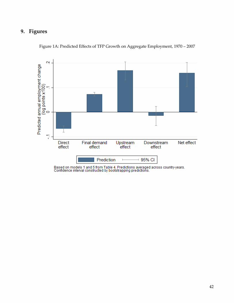
42

9. Figures

Figure 1A: Predicted Effects of TFP Growth on Aggregate Employment, 1970 – 2007

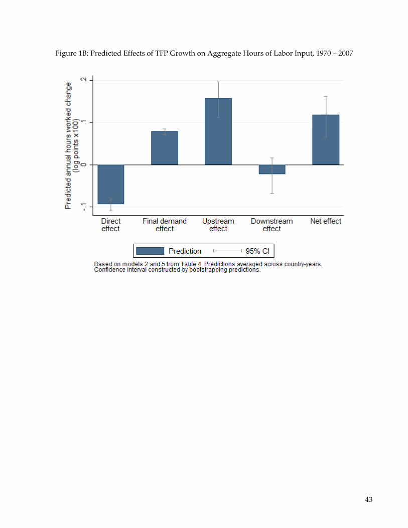
43

Figure 1B: Predicted Effects of TFP Growth on Aggregate Hours of Labor Input, 1970 – 2007

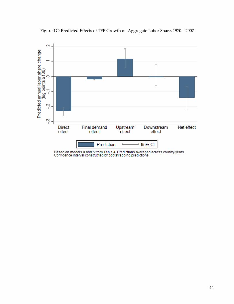
44

Figure 1C: Predicted Effects of TFP Growth on Aggregate Labor Share, 1970 – 2007

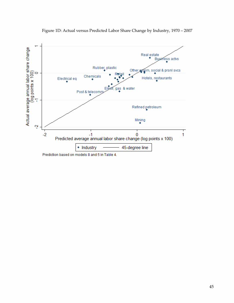
45

Figure 1D: Actual versus Predicted Labor Share Change by Industry, 1970 – 2007

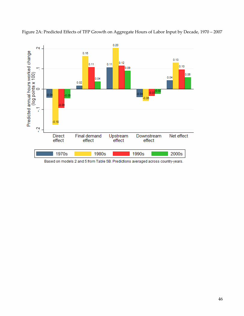
46

Figure 2A: Predicted Effects of TFP Growth on Aggregate Hours of Labor Input by Decade, 1970 – 2007

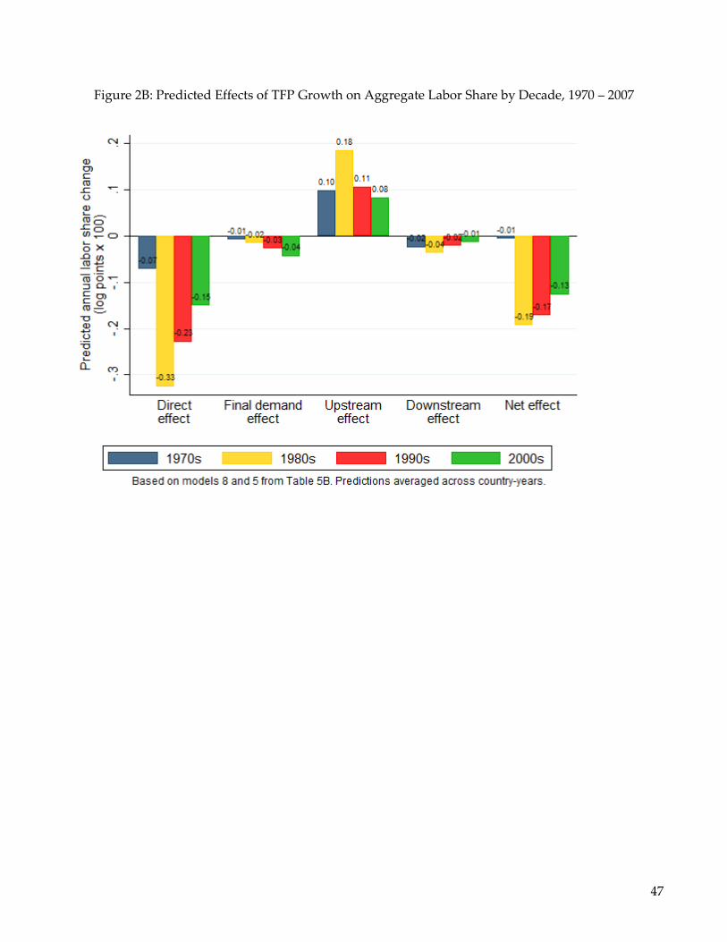
47

Figure 2B: Predicted Effects of TFP Growth on Aggregate Labor Share by Decade, 1970 – 2007

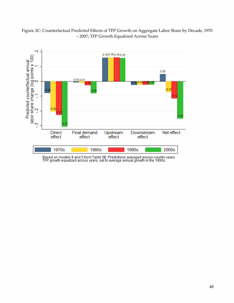
48

Figure 2C: Counterfactual Predicted Effects of TFP Growth on Aggregate Labor Share by Decade, 1970

– 2007; TFP Growth Equalized Across Years

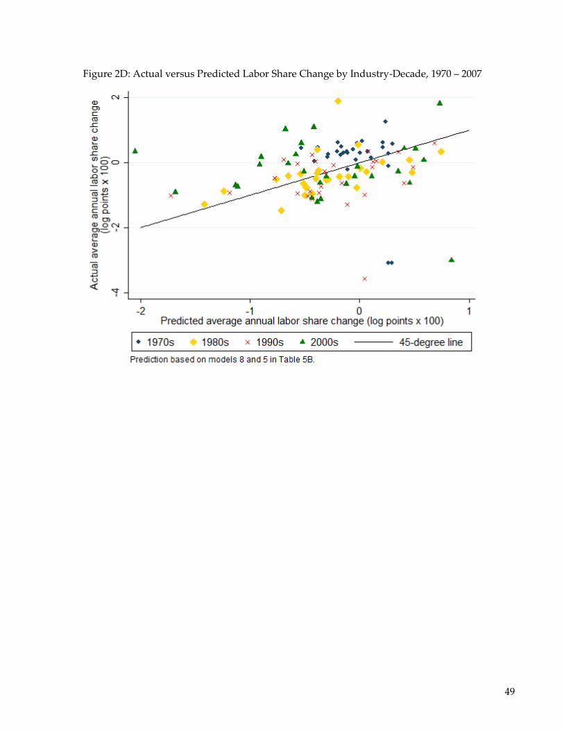
49

Figure 2D: Actual versus Predicted Labor Share Change by Industry-Decade, 1970 – 2007

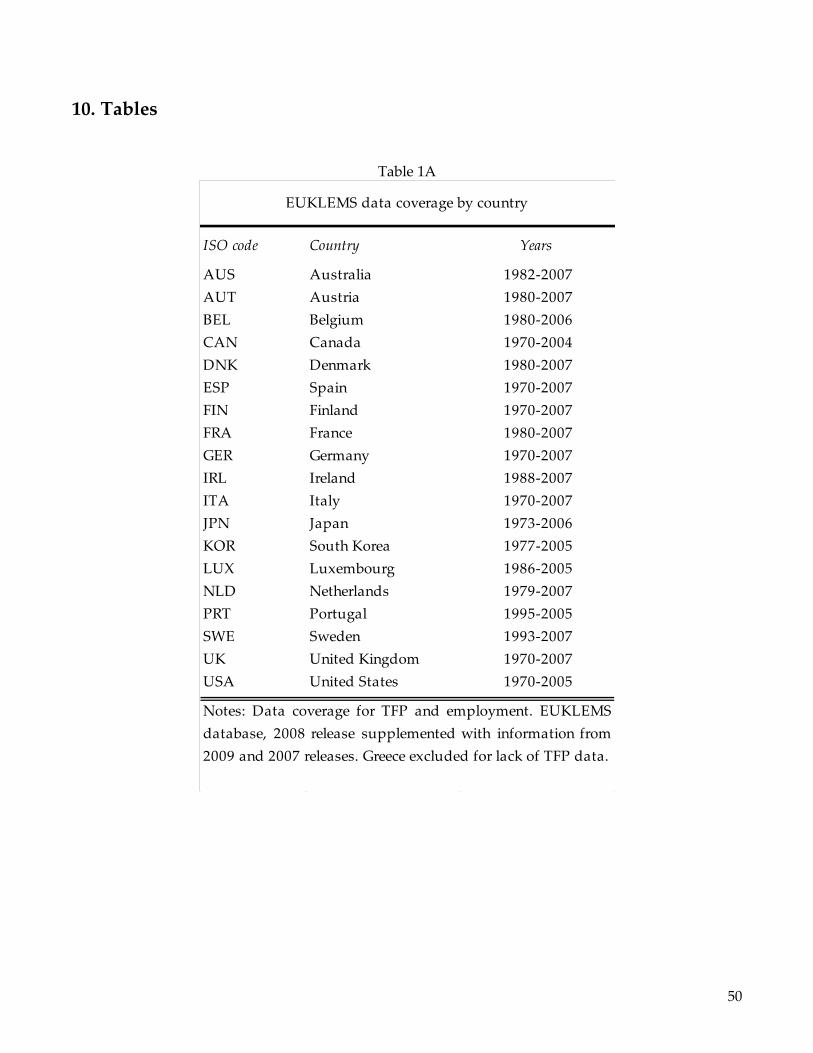
50

10. Tables

Table 1A

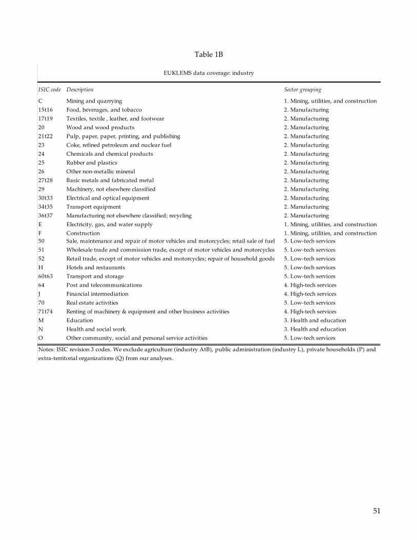
51

Table 1B

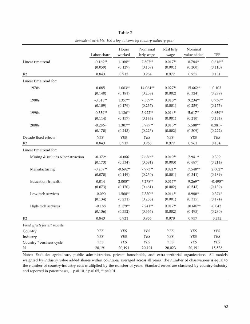
52

Table 2

Linear timetrend -0.169** 1.108** 7.507** 0.017** 8.784** 0.616**

(0.059) (0.129) (0.159) (0.001) (0.200) (0.110)

R2 0.843 0.913 0.954 0.977 0.955 0.131

Linear timetrend for:

1970s 0.085 1.683** 14.064** 0.027** 15.662** -0.103

(0.140) (0.181) (0.258) (0.002) (0.324) (0.289)

1980s -0.318** 1.357** 7.559** 0.018** 9.234** 0.936**

(0.109) (0.179) (0.237) (0.001) (0.259) (0.175)

1990s -0.559** 1.136** 3.922** 0.014** 5.617** 0.659**

(0.114) (0.157) (0.144) (0.001) (0.210) (0.134)

2000s -0.286~ 1.307** 3.987** 0.015** 5.580** 0.381~

(0.170) (0.243) (0.225) (0.002) (0.309) (0.222)

YES YES YES YES YES YES

R2 0.843 0.913 0.965 0.977 0.961 0.134

Linear timetrend for:

Mining & utilities & construction -0.372* -0.066 7.636** 0.019** 7.941** 0.309

(0.173) (0.334) (0.581) (0.003) (0.687) (0.214)

Manufacturing -0.259** -0.692** 7.973** 0.021** 7.540** 2.002**

(0.070) (0.149) (0.230) (0.001) (0.341) (0.189)

Education & health 0.014 2.005** 7.278** 0.017** 9.269** -0.495**

(0.073) (0.170) (0.461) (0.002) (0.543) (0.139)

Low-tech services -0.090 1.560** 7.330** 0.014** 8.980** 0.374*

(0.134) (0.221) (0.258) (0.001) (0.315) (0.174)

High-tech services -0.188 3.179** 7.241** 0.017** 10.607** -0.042

(0.136) (0.352) (0.366) (0.002) (0.495) (0.280)

R2 0.843 0.921 0.955 0.978 0.957 0.242

Country YES YES YES YES YES YES

Industry YES YES YES YES YES YES

Country * business cycle YES YES YES YES YES YES

N 20,191 20,191 20,191 20,023 20,191 15,538

dependent variable: 100 x log outcome by country-industry-year

Notes: Excludes agriculture, public administration, private households, and extra-territorial organizations. All models

weighted by industry value added shares within countries, averaged across all years. The number of observations is equal to

the number of country-industry cells multiplied by the number of years. Standard errors are clustered by country-industry

and reported in parentheses, ~ p<0.10, * p<0.05, ** p<0.01.

Decade fixed effects

Fixed effects for all models:

TFP

Nominal

value added

Real hrly

wage

Nomimal

hrly wage

Hours

workedLabor share

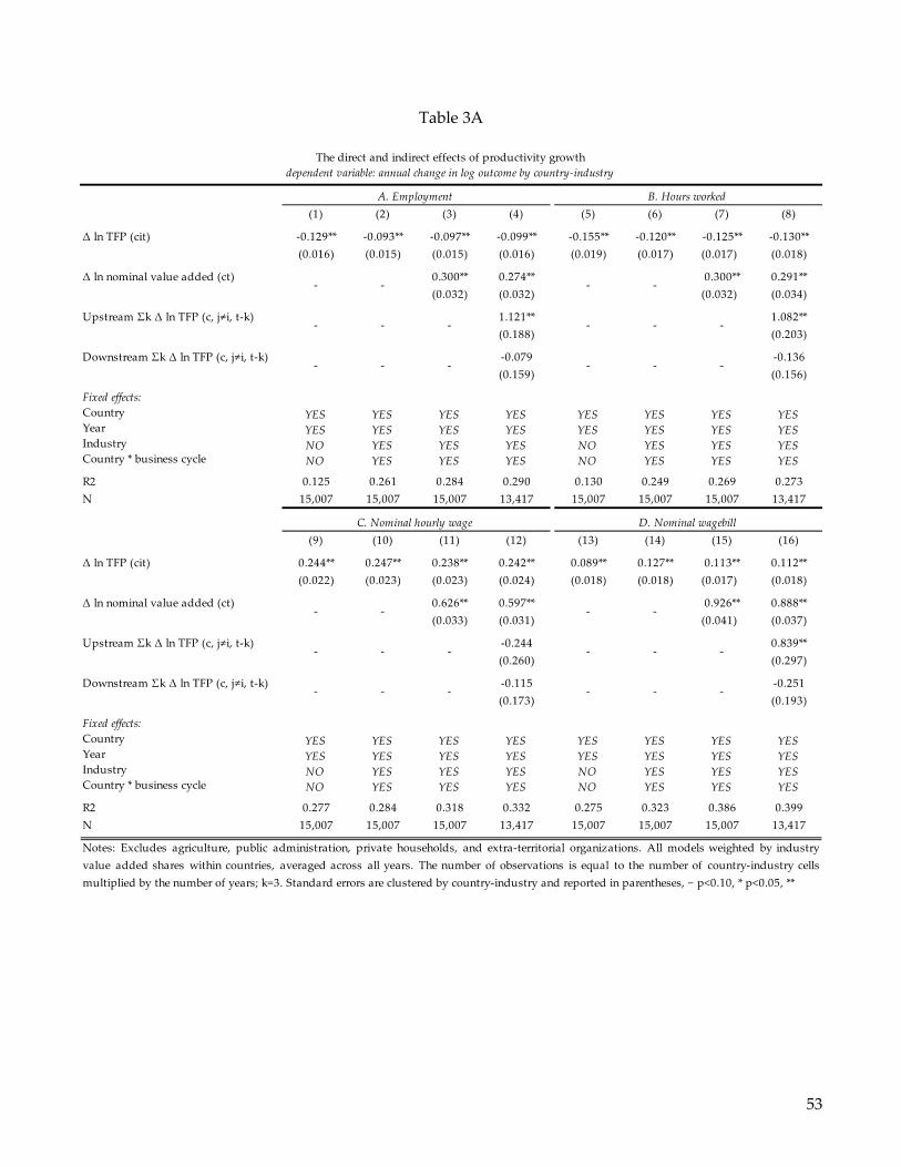
53

Table 3A

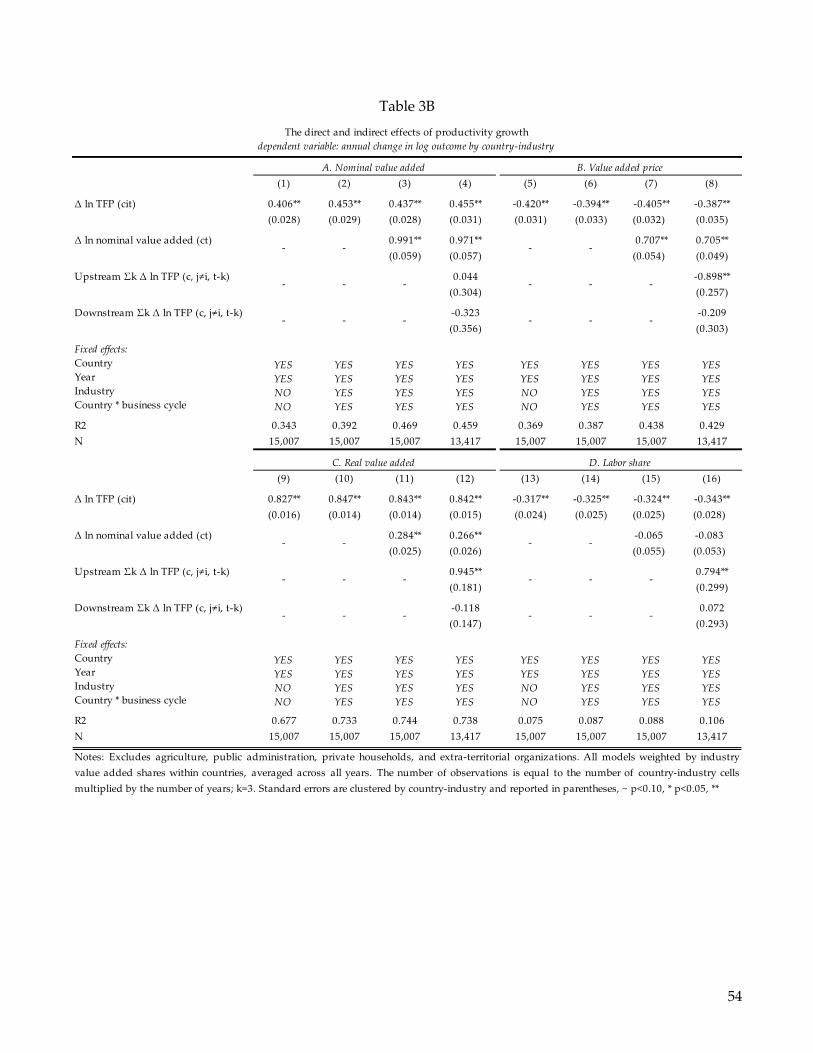
54

Table 3B

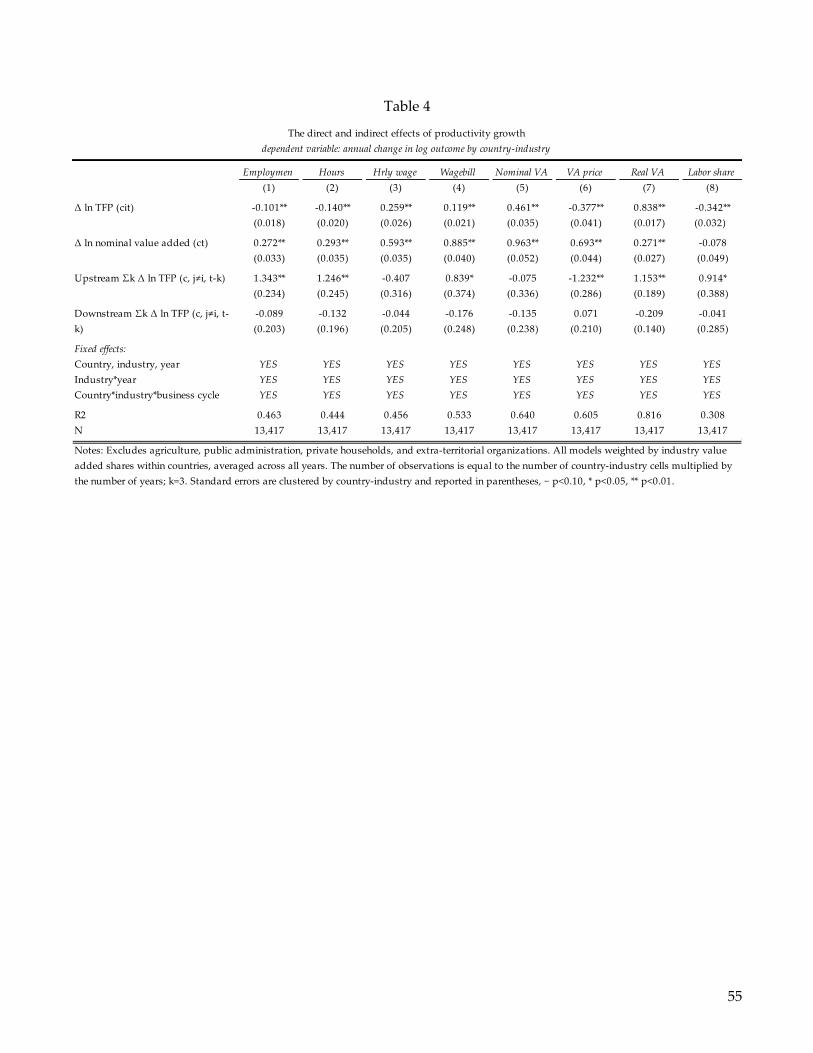
55

Table 4

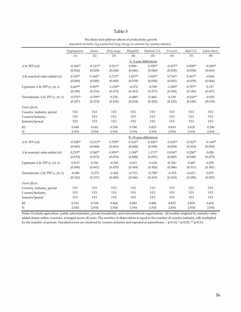
56

Table 5

Employment Hours Hrly wage Wagebill Nominal VA VA price Real VA Labor share

(1) (2) (3) (4) (5) (6) (7) (8)

Δ ln TFP (cit) -0.106** -0.121** 0.211** 0.090~ 0.350** -0.477** 0.828** -0.260**

(0.024) (0.028) (0.048) (0.046) (0.040) (0.050) (0.030) (0.043)

Δ ln nominal value added (ct) 0.335** 0.342** 0.715** 1.057** 1.083** 0.716** 0.367** -0.026

(0.049) (0.049) (0.069) (0.078) (0.058) (0.043) (0.039) (0.064)

Upstream Δ ln TFP (c, j≠i, t) 0.607** 0.957** -1.230** -0.272 -0.399 -1.200** 0.797** 0.127

(0.189) (0.216) (0.475) (0.443) (0.317) (0.294) (0.186) (0.407)

Downstream Δ ln TFP (c, j≠i, t) -0.576** -0.709** 0.230 -0.480* -0.460~ 0.158 -0.616** -0.020

(0.207) (0.219) (0.236) (0.234) (0.243) (0.232) (0.180) (0.210)

Fixed effects:

Country, industry, period YES YES YES YES YES YES YES YES

Country*industry YES YES YES YES YES YES YES YES

Industry*period YES YES YES YES YES YES YES YES

R2 0.648 0.641 0.706 0.760 0.823 0.819 0.830 0.296

N 2,934 2,934 2,934 2,934 2,934 2,934 2,934 2,934

Δ ln TFP (cit) -0.208** -0.213** 0.378** 0.165** 0.326** -0.435** 0.762** -0.160**

(0.045) (0.044) (0.063) (0.048) (0.048) (0.054) (0.034) (0.050)

Δ ln nominal value added (ct) 0.233** 0.240** 0.959** 1.199** 1.171** 0.914** 0.258** 0.028

(0.074) (0.072) (0.076) (0.088) (0.091) (0.083) (0.049) (0.075)

Upstream Δ ln TFP (c, j≠i, t) 0.913* 0.726 -0.705 0.021 -0.238 -0.736~ 0.487 0.259

(0.458) (0.447) (0.475) (0.569) (0.450) (0.386) (0.311) (0.381)

Downstream Δ ln TFP (c, j≠i, t) -0.496 -0.273 -0.442 -0.715~ -0.790* -0.355 -0.431~ 0.075

(0.342) (0.337) (0.408) (0.366) (0.365) (0.365) (0.250) (0.307)

Fixed effects:

Country, industry, period YES YES YES YES YES YES YES YES

Country*industry YES YES YES YES YES YES YES YES

Industry*period YES YES YES YES YES YES YES YES

R2 0.741 0.749 0.864 0.892 0.886 0.873 0.876 0.418

N 2,934 2,934 2,934 2,934 2,934 2,934 2,934 2,934

Notes: Excludes agriculture, public administration, private households, and extra-territorial organizations. All models weighted by industry value

added shares within countries, averaged across all years. The number of observations is equal to the number of country-industry cells multiplied

by the number of periods. Standard errors are clustered by country-industry and reported in parentheses, ~ p<0.10, * p<0.05, ** p<0.01.

A. 5-year differences

B. 10-year differences

The direct and spillover effects of productivity growth

dependent variable: log annualized long change in outcome by country-industry

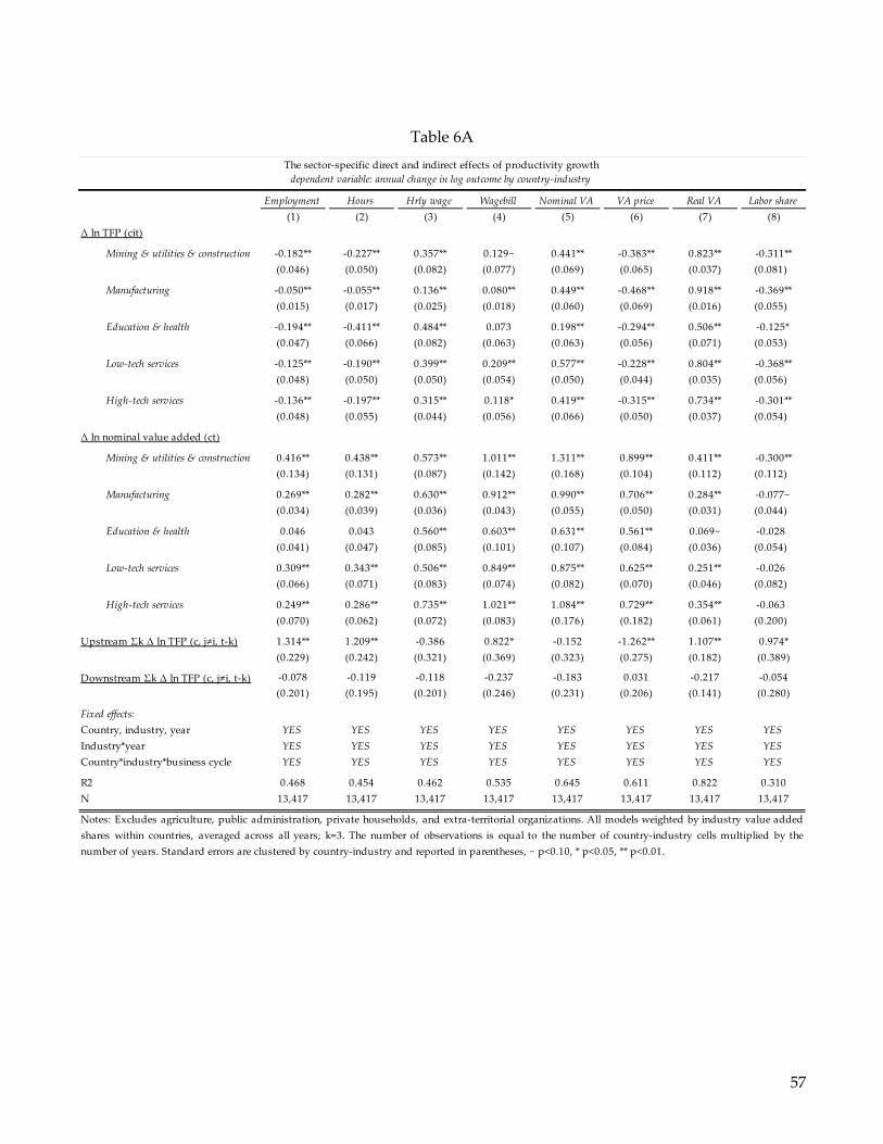
57

Table 6A

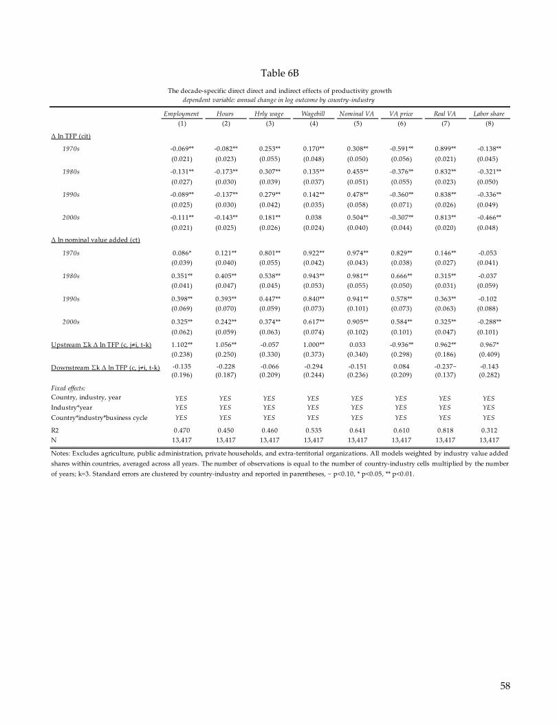
58

Table 6B

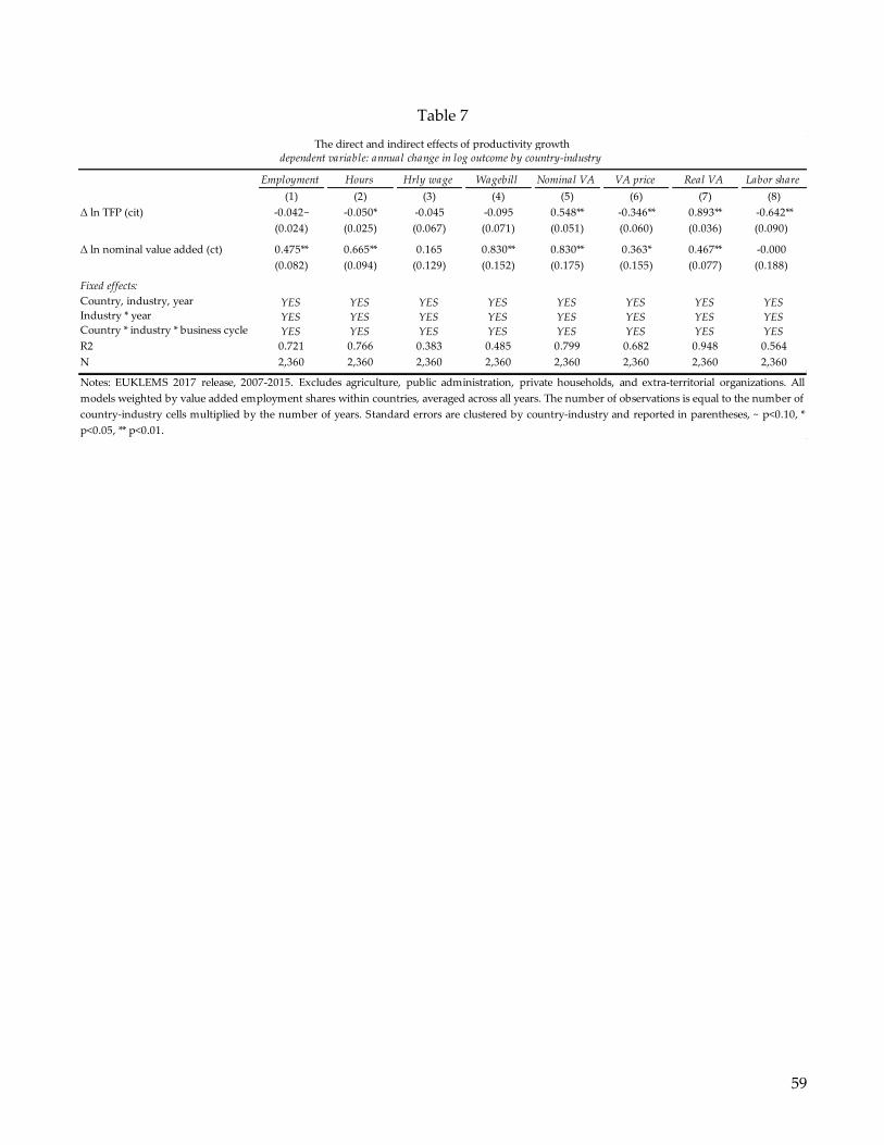
59

Table 7

Employment Hours Hrly wage Wagebill Nominal VA VA price Real VA Labor share

(1) (2) (3) (4) (5) (6) (7) (8)

Δ ln TFP (cit) -0.042~ -0.050* -0.045 -0.095 0.548** -0.346** 0.893** -0.642**

(0.024) (0.025) (0.067) (0.071) (0.051) (0.060) (0.036) (0.090)

Δ ln nominal value added (ct) 0.475** 0.665** 0.165 0.830** 0.830** 0.363* 0.467** -0.000

(0.082) (0.094) (0.129) (0.152) (0.175) (0.155) (0.077) (0.188)

Fixed effects:

Country, industry, year YES YES YES YES YES YES YES YESIndustry * year YES YES YES YES YES YES YES YESCountry * industry * business cycle YES YES YES YES YES YES YES YES

R2 0.721 0.766 0.383 0.485 0.799 0.682 0.948 0.564

N 2,360 2,360 2,360 2,360 2,360 2,360 2,360 2,360

Notes: EUKLEMS 2017 release, 2007-2015. Excludes agriculture, public administration, private households, and extra-territorial organizations. All

models weighted by value added employment shares within countries, averaged across all years. The number of observations is equal to the number of

country-industry cells multiplied by the number of years. Standard errors are clustered by country-industry and reported in parentheses, ~ p<0.10, *

p<0.05, ** p<0.01.

The direct and indirect effects of productivity growthdependent variable: annual change in log outcome by country-industry

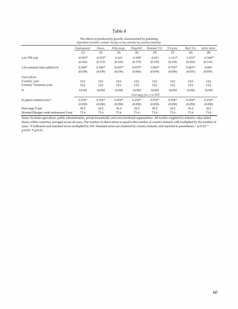
60

Table 8

Employment Hours Hrly wage Wagebill Nominal VA VA price Real VA Labor share

(1) (2) (3) (4) (5) (7) (6) (8)

Δ ln TFP (cit) -0.542** -0.523** 0.165 -0.358* -0.011 -1.111** 1.101** -0.348**

(0.166) (0.172) (0.102) (0.179) (0.155) (0.124) (0.202) (0.116)

Δ ln nominal value added (ct) 0.344** 0.340** 0.633** 0.973** 1.036** 0.776** 0.261** -0.063

(0.038) (0.039) (0.036) (0.046) (0.059) (0.056) (0.031) (0.055)

Fixed effects:

Country, year YES YES YES YES YES YES YES YESCountry * business cycle YES YES YES YES YES YES YES YES

N 14,942 14,942 14,942 14,942 14,942 14,942 14,942 14,942

ln patent citations (cit) ^ 0.254** 0.254** 0.254** 0.254** 0.254** 0.254** 0.254** 0.254**

(0.050) (0.050) (0.050) (0.050) (0.050) (0.050) (0.050) (0.050)

First-stage F-stat 26.2 26.2 26.2 26.2 26.2 26.2 26.2 26.2

Montiel-Pflueger weak instrument F-stat 71.6 71.6 71.6 71.6 71.6 71.6 71.6 71.6

First stage for Δ ln TFP

Notes: Excludes agriculture, public administration, private households, and extra-territorial organizations. All models weighted by industry value added

shares within countries, averaged across all years. The number of observations is equal to the number of country-industry cells multiplied by the number of

years. ^Coefficients and standard errors multiplied by 100. Standard errors are clustered by country-industry and reported in parentheses, ~ p<0.10, *

p<0.05, ** p<0.01.

The effects of productivity growth, instrumented by patentingdependent variable: annual change in log outcome by country-industry

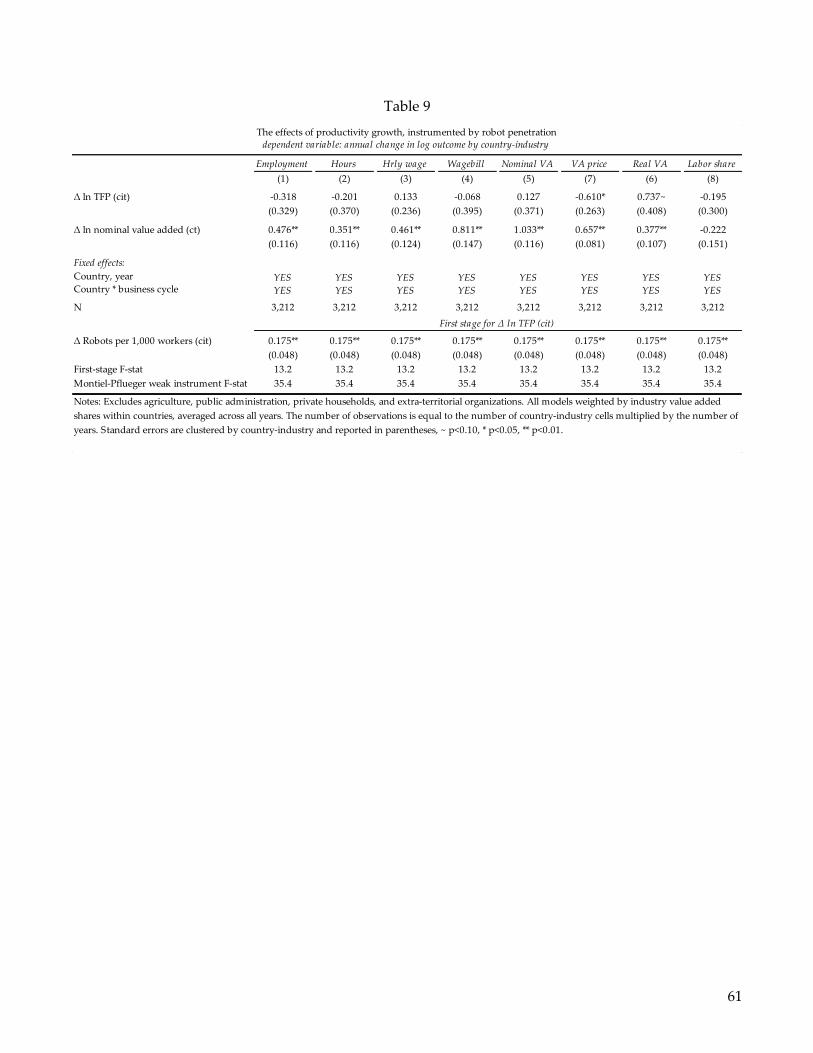
61

Table 9

Employment Hours Hrly wage Wagebill Nominal VA VA price Real VA Labor share

(1) (2) (3) (4) (5) (7) (6) (8)

Δ ln TFP (cit) -0.318 -0.201 0.133 -0.068 0.127 -0.610* 0.737~ -0.195

(0.329) (0.370) (0.236) (0.395) (0.371) (0.263) (0.408) (0.300)

Δ ln nominal value added (ct) 0.476** 0.351** 0.461** 0.811** 1.033** 0.657** 0.377** -0.222

(0.116) (0.116) (0.124) (0.147) (0.116) (0.081) (0.107) (0.151)

Fixed effects:

Country, year YES YES YES YES YES YES YES YESCountry * business cycle YES YES YES YES YES YES YES YES

N 3,212 3,212 3,212 3,212 3,212 3,212 3,212 3,212

Δ Robots per 1,000 workers (cit) 0.175** 0.175** 0.175** 0.175** 0.175** 0.175** 0.175** 0.175**

(0.048) (0.048) (0.048) (0.048) (0.048) (0.048) (0.048) (0.048)

First-stage F-stat 13.2 13.2 13.2 13.2 13.2 13.2 13.2 13.2

Montiel-Pflueger weak instrument F-stat 35.4 35.4 35.4 35.4 35.4 35.4 35.4 35.4

The effects of productivity growth, instrumented by robot penetrationdependent variable: annual change in log outcome by country-industry

First stage for Δ ln TFP (cit)

Notes: Excludes agriculture, public administration, private households, and extra-territorial organizations. All models weighted by industry value added

shares within countries, averaged across all years. The number of observations is equal to the number of country-industry cells multiplied by the number of

years. Standard errors are clustered by country-industry and reported in parentheses, ~ p<0.10, * p<0.05, ** p<0.01.

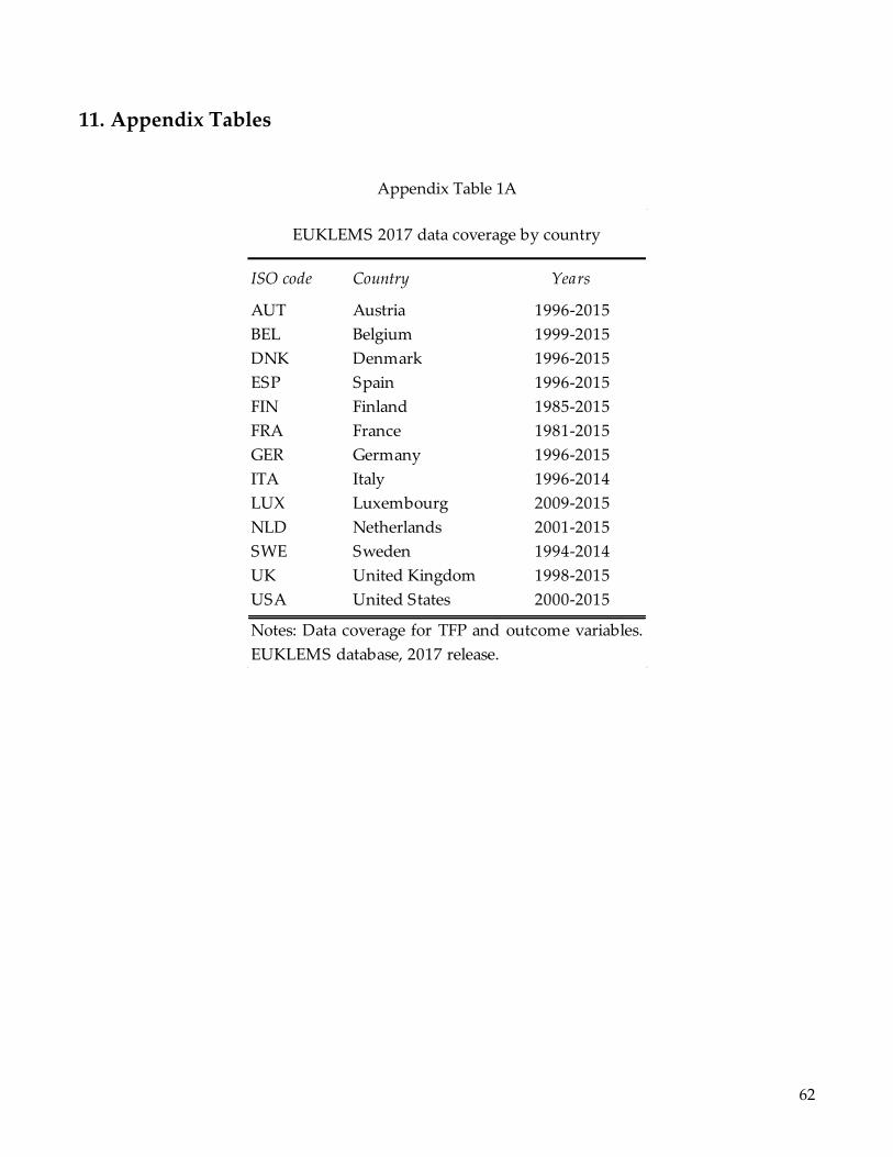
62

11. Appendix Tables

Appendix Table 1A

Country

AUT Austria 1996-2015

BEL Belgium 1999-2015

DNK Denmark 1996-2015

ESP Spain 1996-2015

FIN Finland 1985-2015

FRA France 1981-2015

GER Germany 1996-2015

ITA Italy 1996-2014

LUX Luxembourg 2009-2015

NLD Netherlands 2001-2015

SWE Sweden 1994-2014

UK United Kingdom 1998-2015

USA United States 2000-2015

EUKLEMS 2017 data coverage by country

ISO code Years

Notes: Data coverage for TFP and outcome variables.

EUKLEMS database, 2017 release.

63

Appendix Table 1B

ISIC code Description

B Mining and quarrying

10-12 Food products, beverages and tobacco

13-15 Textiles, wearing apparel, leather and related prodcuts

16-18 Wood and paper products; printing and reproduction of recorded media

19 Coke and refined petroleum products

20-21 Chemicals and chemical products

22-23 Rubber and plastics products, and other non-metallic mineral products

24-25 Basic metals and fabricated metal products, except machinery and equipment

26-27 Electrical and optical equipment

28 Machinery and equipment n.e.c.

29-30 Transport equipment

31-33 Other manufacturing; repair and installation of machinery and equipment

D-E Electricity, gas and water supply

F Construction

G Wholesale and retail trade; repair of motor vehicles and motorcycles

H Transportation and storage

I Accommodation and food service activities

J Information and communication

K Financial and insurance activities

L Real estate activities

M-N Professional, scientific, technical, administrative and support service activities

P Education

Q Health and social work

R-S Arts, entertainment, recreation and other service activities

EUKLEMS 2017 data coverage: industry

Notes: ISIC revision 4 codes. We exclude Agriculture, forestry and fishing (industry A), public

administration (industry O), and private households (T) and extra-territorial organizations (U)

from our analyses. Industries 10-12 through 31-33 are manufacturing industries.

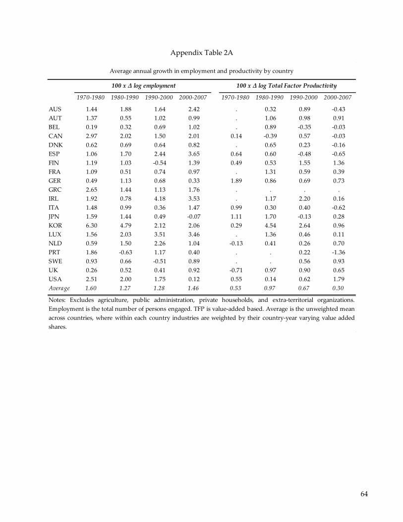
64

Appendix Table 2A

1970-1980 1980-1990 1990-2000 2000-2007 1970-1980 1980-1990 1990-2000 2000-2007

AUS 1.44 1.88 1.64 2.42 . 0.32 0.89 -0.43

AUT 1.37 0.55 1.02 0.99 . 1.06 0.98 0.91

BEL 0.19 0.32 0.69 1.02 . 0.89 -0.35 -0.03

CAN 2.97 2.02 1.50 2.01 0.14 -0.39 0.57 -0.03

DNK 0.62 0.69 0.64 0.82 . 0.65 0.23 -0.16

ESP 1.06 1.70 2.44 3.65 0.64 0.60 -0.48 -0.65

FIN 1.19 1.03 -0.54 1.39 0.49 0.53 1.55 1.36

FRA 1.09 0.51 0.74 0.97 . 1.31 0.59 0.39

GER 0.49 1.13 0.68 0.33 1.89 0.86 0.69 0.73

GRC 2.65 1.44 1.13 1.76 . . . .

IRL 1.92 0.78 4.18 3.53 . 1.17 2.20 0.16

ITA 1.48 0.99 0.36 1.47 0.99 0.30 0.40 -0.62

JPN 1.59 1.44 0.49 -0.07 1.11 1.70 -0.13 0.28

KOR 6.30 4.79 2.12 2.06 0.29 4.54 2.64 0.96

LUX 1.56 2.03 3.51 3.46 . 1.36 0.46 0.11

NLD 0.59 1.50 2.26 1.04 -0.13 0.41 0.26 0.70

PRT 1.86 -0.63 1.17 0.40 . . 0.22 -1.36

SWE 0.93 0.66 -0.51 0.89 . . 0.56 0.93

UK 0.26 0.52 0.41 0.92 -0.71 0.97 0.90 0.65

USA 2.51 2.00 1.75 0.12 0.55 0.14 0.62 1.79

Average 1.60 1.27 1.28 1.46 0.53 0.97 0.67 0.30

Notes: Excludes agriculture, public administration, private households, and extra-territorial organizations.

Employment is the total number of persons engaged. TFP is value-added based. Average is the unweighted mean

across countries, where within each country industries are weighted by their country-year varying value added

shares.

Average annual growth in employment and productivity by country

100 x Δ log employment 100 x Δ log Total Factor Productivity

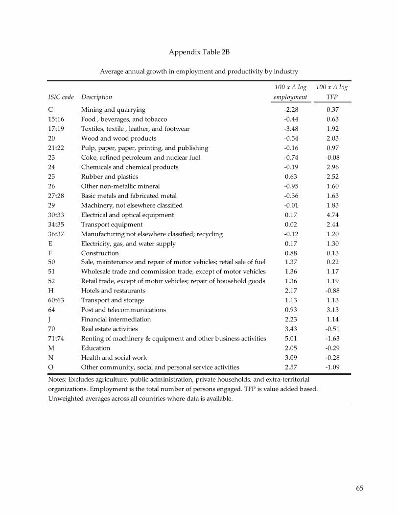
65

Appendix Table 2B

ISIC code Description

C Mining and quarrying -2.28 0.37

15t16 Food , beverages, and tobacco -0.44 0.63

17t19 Textiles, textile , leather, and footwear -3.48 1.92

20 Wood and wood products -0.54 2.03

21t22 Pulp, paper, paper, printing, and publishing -0.16 0.97

23 Coke, refined petroleum and nuclear fuel -0.74 -0.08

24 Chemicals and chemical products -0.19 2.96

25 Rubber and plastics 0.63 2.52

26 Other non-metallic mineral -0.95 1.60

27t28 Basic metals and fabricated metal -0.36 1.63

29 Machinery, not elsewhere classified -0.01 1.83

30t33 Electrical and optical equipment 0.17 4.74

34t35 Transport equipment 0.02 2.44

36t37 Manufacturing not elsewhere classified; recycling -0.12 1.20

E Electricity, gas, and water supply 0.17 1.30

F Construction 0.88 0.13

50 Sale, maintenance and repair of motor vehicles; retail sale of fuel 1.37 0.22

51 Wholesale trade and commission trade, except of motor vehicles 1.36 1.17

52 Retail trade, except of motor vehicles; repair of household goods 1.36 1.19

H Hotels and restaurants 2.17 -0.88

60t63 Transport and storage 1.13 1.13

64 Post and telecommunications 0.93 3.13

J Financial intermediation 2.23 1.14

70 Real estate activities 3.43 -0.51

71t74 Renting of machinery & equipment and other business activities 5.01 -1.63

M Education 2.05 -0.29

N Health and social work 3.09 -0.28

O Other community, social and personal service activities 2.57 -1.09

Average annual growth in employment and productivity by industry

Notes: Excludes agriculture, public administration, private households, and extra-territorial

organizations. Employment is the total number of persons engaged. TFP is value added based.

Unweighted averages across all countries where data is available.

100 x Δ log

employment

100 x Δ log

TFP

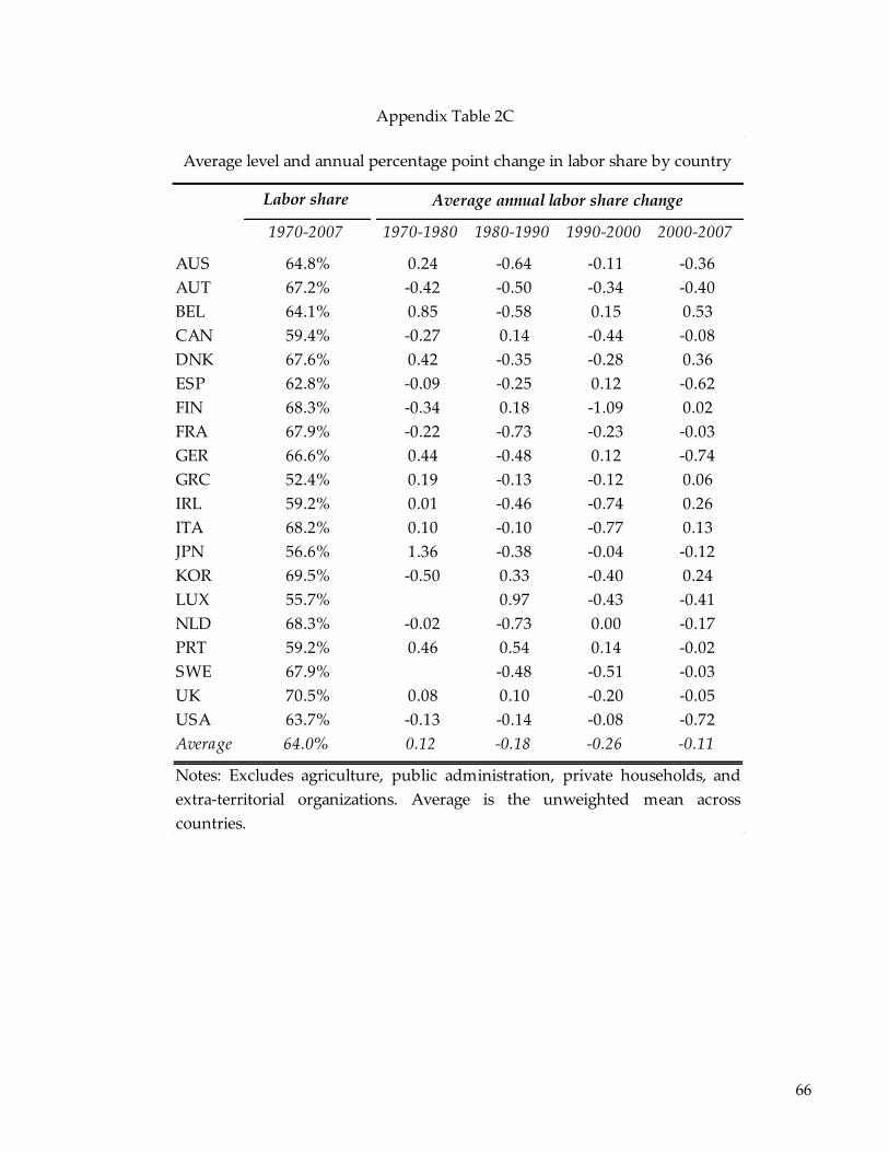
66

Appendix Table 2C

Labor share

1970-2007 1970-1980 1980-1990 1990-2000 2000-2007

AUS 64.8% 0.24 -0.64 -0.11 -0.36

AUT 67.2% -0.42 -0.50 -0.34 -0.40

BEL 64.1% 0.85 -0.58 0.15 0.53

CAN 59.4% -0.27 0.14 -0.44 -0.08

DNK 67.6% 0.42 -0.35 -0.28 0.36

ESP 62.8% -0.09 -0.25 0.12 -0.62

FIN 68.3% -0.34 0.18 -1.09 0.02

FRA 67.9% -0.22 -0.73 -0.23 -0.03

GER 66.6% 0.44 -0.48 0.12 -0.74

GRC 52.4% 0.19 -0.13 -0.12 0.06

IRL 59.2% 0.01 -0.46 -0.74 0.26

ITA 68.2% 0.10 -0.10 -0.77 0.13

JPN 56.6% 1.36 -0.38 -0.04 -0.12

KOR 69.5% -0.50 0.33 -0.40 0.24

LUX 55.7% 0.97 -0.43 -0.41

NLD 68.3% -0.02 -0.73 0.00 -0.17

PRT 59.2% 0.46 0.54 0.14 -0.02

SWE 67.9% -0.48 -0.51 -0.03

UK 70.5% 0.08 0.10 -0.20 -0.05

USA 63.7% -0.13 -0.14 -0.08 -0.72

Average 64.0% 0.12 -0.18 -0.26 -0.11

Average annual labor share change

Average level and annual percentage point change in labor share by country

Notes: Excludes agriculture, public administration, private households, and

extra-territorial organizations. Average is the unweighted mean across

countries.

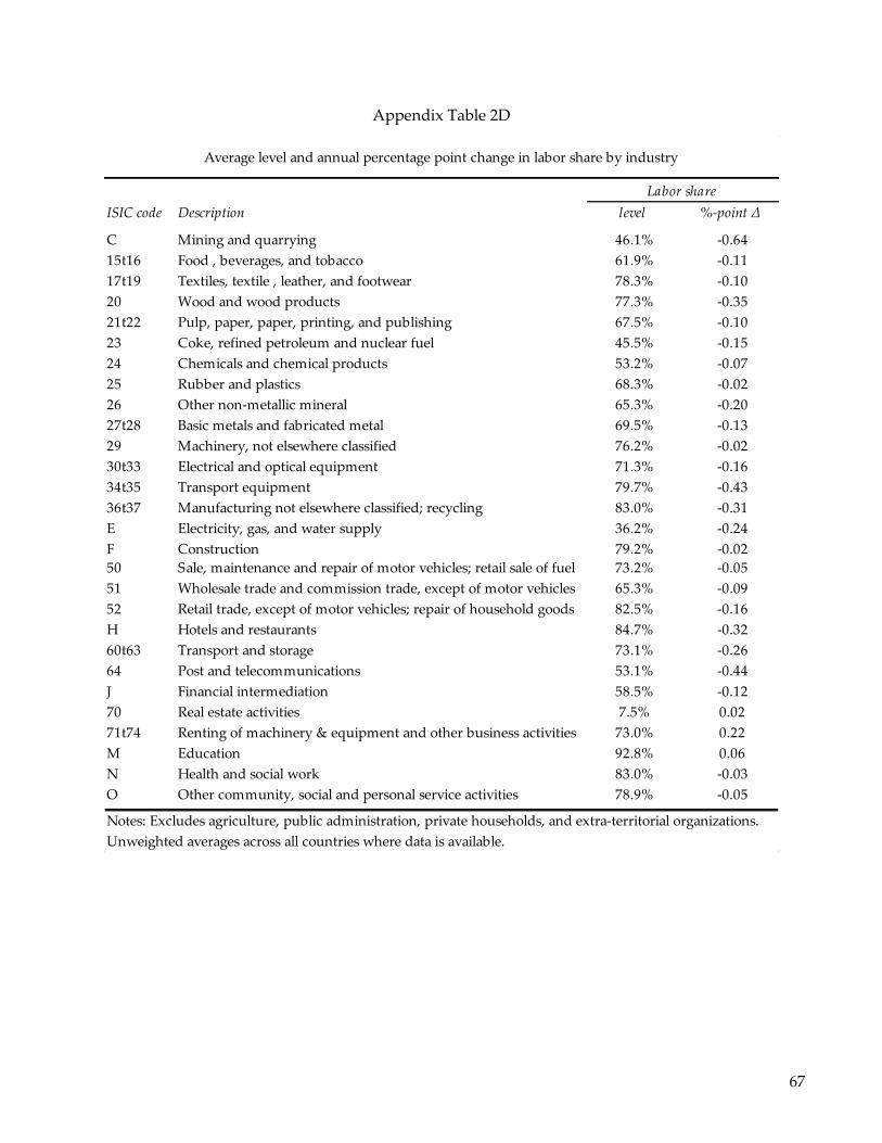
67

Appendix Table 2D

ISIC code Description level %-point Δ

C Mining and quarrying 46.1% -0.64

15t16 Food , beverages, and tobacco 61.9% -0.11

17t19 Textiles, textile , leather, and footwear 78.3% -0.10

20 Wood and wood products 77.3% -0.35

21t22 Pulp, paper, paper, printing, and publishing 67.5% -0.10

23 Coke, refined petroleum and nuclear fuel 45.5% -0.15

24 Chemicals and chemical products 53.2% -0.07

25 Rubber and plastics 68.3% -0.02

26 Other non-metallic mineral 65.3% -0.20

27t28 Basic metals and fabricated metal 69.5% -0.13

29 Machinery, not elsewhere classified 76.2% -0.02

30t33 Electrical and optical equipment 71.3% -0.16

34t35 Transport equipment 79.7% -0.43

36t37 Manufacturing not elsewhere classified; recycling 83.0% -0.31

E Electricity, gas, and water supply 36.2% -0.24

F Construction 79.2% -0.02

50 Sale, maintenance and repair of motor vehicles; retail sale of fuel 73.2% -0.05

51 Wholesale trade and commission trade, except of motor vehicles 65.3% -0.09

52 Retail trade, except of motor vehicles; repair of household goods 82.5% -0.16

H Hotels and restaurants 84.7% -0.32

60t63 Transport and storage 73.1% -0.26

64 Post and telecommunications 53.1% -0.44

J Financial intermediation 58.5% -0.12

70 Real estate activities 7.5% 0.02

71t74 Renting of machinery & equipment and other business activities 73.0% 0.22

M Education 92.8% 0.06

N Health and social work 83.0% -0.03

O Other community, social and personal service activities 78.9% -0.05

Notes: Excludes agriculture, public administration, private households, and extra-territorial organizations.

Unweighted averages across all countries where data is available.

Average level and annual percentage point change in labor share by industry

Labor share

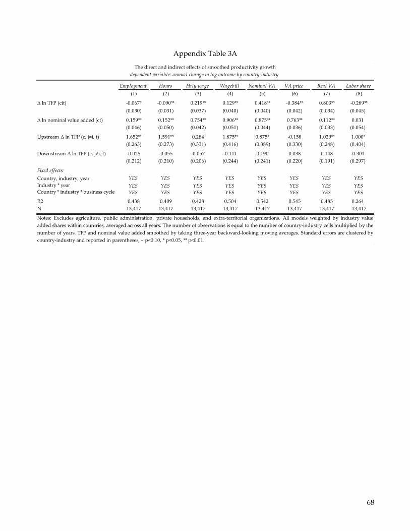
68

Appendix Table 3A

Employment Hours Hrly wage Wagebill Nominal VA VA price Real VA Labor share

(1) (2) (3) (4) (5) (6) (7) (8)

-0.067* -0.090** 0.219** 0.129** 0.418** -0.384** 0.803** -0.289**

(0.030) (0.031) (0.037) (0.040) (0.040) (0.042) (0.034) (0.045)

0.159** 0.152** 0.754** 0.906** 0.875** 0.763** 0.112** 0.031

(0.046) (0.050) (0.042) (0.051) (0.044) (0.036) (0.033) (0.054)

1.652** 1.591** 0.284 1.875** 0.875* -0.158 1.029** 1.000*

(0.263) (0.273) (0.331) (0.416) (0.389) (0.330) (0.248) (0.404)

-0.025 -0.055 -0.057 -0.111 0.190 0.038 0.148 -0.301

(0.212) (0.210) (0.206) (0.244) (0.241) (0.220) (0.191) (0.297)

Fixed effects:

Country, industry, year YES YES YES YES YES YES YES YES

Industry * year YES YES YES YES YES YES YES YESCountry * industry * business cycle YES YES YES YES YES YES YES YES

R2 0.438 0.409 0.428 0.504 0.542 0.545 0.485 0.264

N 13,417 13,417 13,417 13,417 13,417 13,417 13,417 13,417

Notes: Excludes agriculture, public administration, private households, and extra-territorial organizations. All models weighted by industry value

added shares within countries, averaged across all years. The number of observations is equal to the number of country-industry cells multiplied by the

number of years. TFP and nominal value added smoothed by taking three-year backward-looking moving averages. Standard errors are clustered by

country-industry and reported in parentheses, ~ p<0.10, * p<0.05, ** p<0.01.

Upstream Δ ln TFP (c, j≠i, t)

Downstream Δ ln TFP (c, j≠i, t)

Δ ln nominal value added (ct)

The direct and indirect effects of smoothed productivity growth

dependent variable: annual change in log outcome by country-industry

Δ ln TFP (cit)

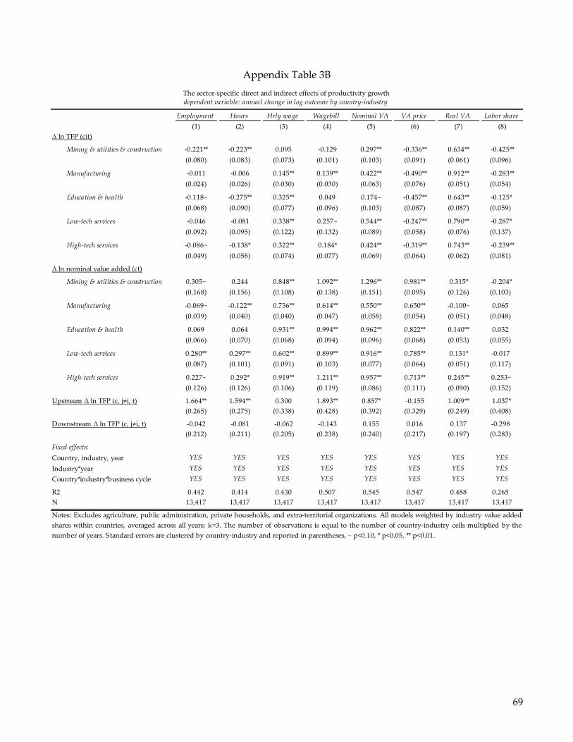
69

Appendix Table 3B

Employment Hours Hrly wage Wagebill Nominal VA VA price Real VA Labor share

(1) (2) (3) (4) (5) (6) (7) (8)

Mining & utilities & construction -0.221** -0.223** 0.095 -0.129 0.297** -0.336** 0.634** -0.425**

(0.080) (0.083) (0.073) (0.101) (0.103) (0.091) (0.061) (0.096)

Manufacturing -0.011 -0.006 0.145** 0.139** 0.422** -0.490** 0.912** -0.283**

(0.024) (0.026) (0.030) (0.030) (0.063) (0.076) (0.051) (0.054)

Education & health -0.118~ -0.275** 0.325** 0.049 0.174~ -0.457** 0.643** -0.125*

(0.068) (0.090) (0.077) (0.096) (0.103) (0.087) (0.087) (0.059)

Low-tech services -0.046 -0.081 0.338** 0.257~ 0.544** -0.247** 0.790** -0.287*

(0.092) (0.095) (0.122) (0.132) (0.089) (0.058) (0.076) (0.137)

High-tech services -0.086~ -0.138* 0.322** 0.184* 0.424** -0.319** 0.743** -0.239**

(0.049) (0.058) (0.074) (0.077) (0.069) (0.064) (0.062) (0.081)

Δ ln nominal value added (ct)

Mining & utilities & construction 0.305~ 0.244 0.848** 1.092** 1.296** 0.981** 0.315* -0.204*

(0.168) (0.156) (0.108) (0.138) (0.151) (0.095) (0.126) (0.103)

Manufacturing -0.069~ -0.122** 0.736** 0.614** 0.550** 0.650** -0.100~ 0.065

(0.039) (0.040) (0.040) (0.047) (0.058) (0.054) (0.051) (0.048)

Education & health 0.069 0.064 0.931** 0.994** 0.962** 0.822** 0.140** 0.032

(0.066) (0.070) (0.068) (0.094) (0.096) (0.068) (0.053) (0.055)

Low-tech services 0.280** 0.297** 0.602** 0.899** 0.916** 0.785** 0.131* -0.017

(0.087) (0.101) (0.091) (0.103) (0.077) (0.064) (0.051) (0.117)

High-tech services 0.227~ 0.292* 0.919** 1.211** 0.957** 0.713** 0.245** 0.253~

(0.126) (0.126) (0.106) (0.119) (0.086) (0.111) (0.090) (0.152)

1.664** 1.594** 0.300 1.893** 0.857* -0.155 1.009** 1.037*

(0.265) (0.275) (0.338) (0.428) (0.392) (0.329) (0.249) (0.408)

-0.042 -0.081 -0.062 -0.143 0.155 0.016 0.137 -0.298

(0.212) (0.211) (0.205) (0.238) (0.240) (0.217) (0.197) (0.283)

Country, industry, year YES YES YES YES YES YES YES YES

Industry*year YES YES YES YES YES YES YES YES

Country*industry*business cycle YES YES YES YES YES YES YES YES

R2 0.442 0.414 0.430 0.507 0.545 0.547 0.488 0.265

N 13,417 13,417 13,417 13,417 13,417 13,417 13,417 13,417

Downstream Δ ln TFP (c, j≠i, t)

Fixed effects:

Notes: Excludes agriculture, public administration, private households, and extra-territorial organizations. All models weighted by industry value added

shares within countries, averaged across all years; k=3. The number of observations is equal to the number of country-industry cells multiplied by the

number of years. Standard errors are clustered by country-industry and reported in parentheses, ~ p<0.10, * p<0.05, ** p<0.01.

The sector-specific direct and indirect effects of productivity growthdependent variable: annual change in log outcome by country-industry

Δ ln TFP (cit)

Upstream Δ ln TFP (c, j≠i, t)

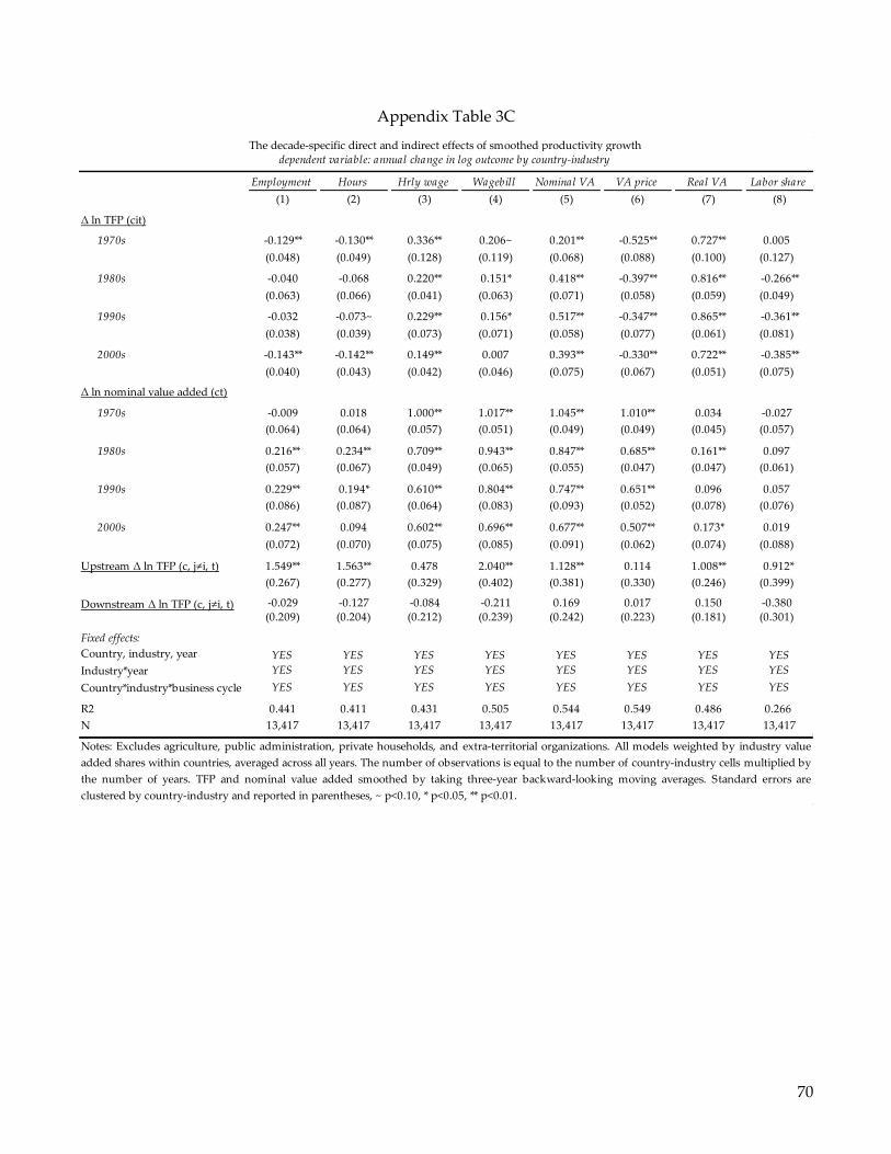
70

Appendix Table 3C

Employment Hours Hrly wage Wagebill Nominal VA VA price Real VA Labor share

(1) (2) (3) (4) (5) (6) (7) (8)

1970s -0.129** -0.130** 0.336** 0.206~ 0.201** -0.525** 0.727** 0.005

(0.048) (0.049) (0.128) (0.119) (0.068) (0.088) (0.100) (0.127)

1980s -0.040 -0.068 0.220** 0.151* 0.418** -0.397** 0.816** -0.266**

(0.063) (0.066) (0.041) (0.063) (0.071) (0.058) (0.059) (0.049)

1990s -0.032 -0.073~ 0.229** 0.156* 0.517** -0.347** 0.865** -0.361**

(0.038) (0.039) (0.073) (0.071) (0.058) (0.077) (0.061) (0.081)

2000s -0.143** -0.142** 0.149** 0.007 0.393** -0.330** 0.722** -0.385**

(0.040) (0.043) (0.042) (0.046) (0.075) (0.067) (0.051) (0.075)

Δ ln nominal value added (ct)

1970s -0.009 0.018 1.000** 1.017** 1.045** 1.010** 0.034 -0.027

(0.064) (0.064) (0.057) (0.051) (0.049) (0.049) (0.045) (0.057)

1980s 0.216** 0.234** 0.709** 0.943** 0.847** 0.685** 0.161** 0.097

(0.057) (0.067) (0.049) (0.065) (0.055) (0.047) (0.047) (0.061)

1990s 0.229** 0.194* 0.610** 0.804** 0.747** 0.651** 0.096 0.057

(0.086) (0.087) (0.064) (0.083) (0.093) (0.052) (0.078) (0.076)

2000s 0.247** 0.094 0.602** 0.696** 0.677** 0.507** 0.173* 0.019

(0.072) (0.070) (0.075) (0.085) (0.091) (0.062) (0.074) (0.088)

1.549** 1.563** 0.478 2.040** 1.128** 0.114 1.008** 0.912*

(0.267) (0.277) (0.329) (0.402) (0.381) (0.330) (0.246) (0.399)

-0.029 -0.127 -0.084 -0.211 0.169 0.017 0.150 -0.380 (0.209) (0.204) (0.212) (0.239) (0.242) (0.223) (0.181) (0.301)

Country, industry, year YES YES YES YES YES YES YES YES

Industry*year YES YES YES YES YES YES YES YES

Country*industry*business cycle YES YES YES YES YES YES YES YES

R2 0.441 0.411 0.431 0.505 0.544 0.549 0.486 0.266

N 13,417 13,417 13,417 13,417 13,417 13,417 13,417 13,417

Downstream Δ ln TFP (c, j≠i, t)

Fixed effects:

Notes: Excludes agriculture, public administration, private households, and extra-territorial organizations. All models weighted by industry value

added shares within countries, averaged across all years. The number of observations is equal to the number of country-industry cells multiplied by

the number of years. TFP and nominal value added smoothed by taking three-year backward-looking moving averages. Standard errors are

clustered by country-industry and reported in parentheses, ~ p<0.10, * p<0.05, ** p<0.01.

The decade-specific direct and indirect effects of smoothed productivity growthdependent variable: annual change in log outcome by country-industry

Δ ln TFP (cit)

Upstream Δ ln TFP (c, j≠i, t)

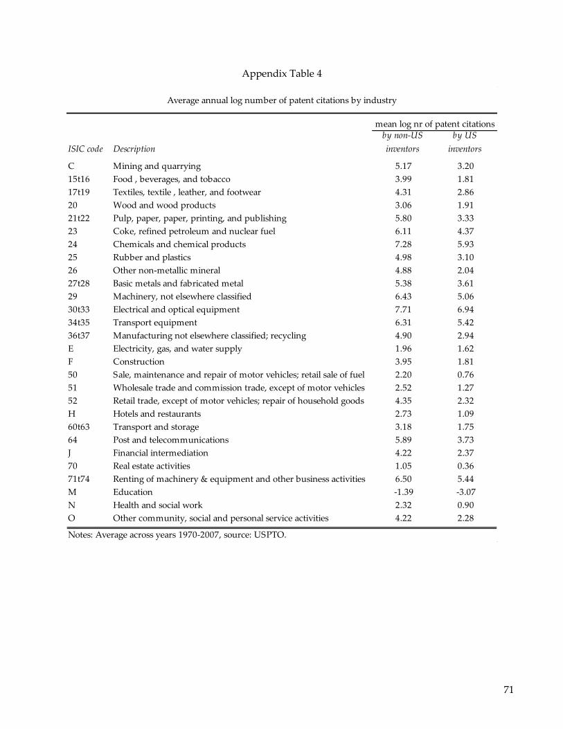
71

Appendix Table 4

ISIC code Description

C Mining and quarrying 5.17 3.20

15t16 Food , beverages, and tobacco 3.99 1.81

17t19 Textiles, textile , leather, and footwear 4.31 2.86

20 Wood and wood products 3.06 1.91

21t22 Pulp, paper, paper, printing, and publishing 5.80 3.33

23 Coke, refined petroleum and nuclear fuel 6.11 4.37

24 Chemicals and chemical products 7.28 5.93

25 Rubber and plastics 4.98 3.10

26 Other non-metallic mineral 4.88 2.04

27t28 Basic metals and fabricated metal 5.38 3.61

29 Machinery, not elsewhere classified 6.43 5.06

30t33 Electrical and optical equipment 7.71 6.94

34t35 Transport equipment 6.31 5.42

36t37 Manufacturing not elsewhere classified; recycling 4.90 2.94

E Electricity, gas, and water supply 1.96 1.62

F Construction 3.95 1.81

50 Sale, maintenance and repair of motor vehicles; retail sale of fuel 2.20 0.76

51 Wholesale trade and commission trade, except of motor vehicles 2.52 1.27

52 Retail trade, except of motor vehicles; repair of household goods 4.35 2.32

H Hotels and restaurants 2.73 1.09

60t63 Transport and storage 3.18 1.75

64 Post and telecommunications 5.89 3.73

J Financial intermediation 4.22 2.37

70 Real estate activities 1.05 0.36

71t74 Renting of machinery & equipment and other business activities 6.50 5.44

M Education -1.39 -3.07

N Health and social work 2.32 0.90

O Other community, social and personal service activities 4.22 2.28

Notes: Average across years 1970-2007, source: USPTO.

Average annual log number of patent citations by industry

mean log nr of patent citationsby non-US

inventors

by US

inventors

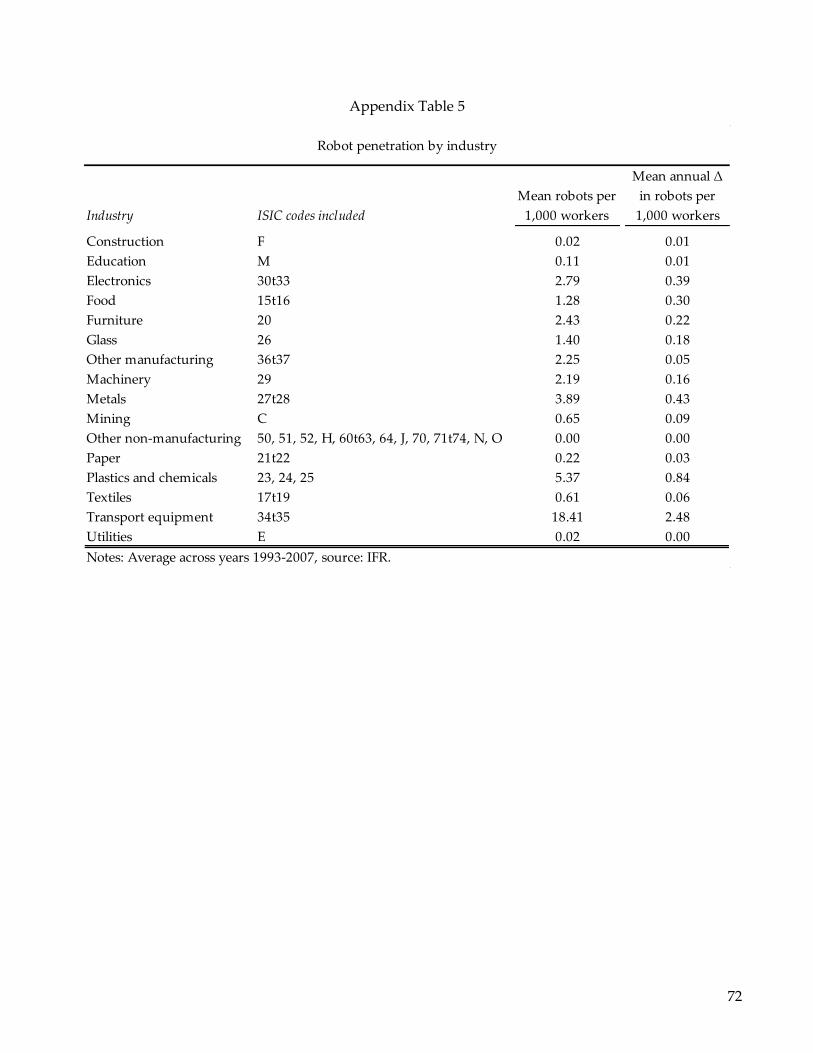
72

Appendix Table 5

Industry ISIC codes included

Construction F 0.02 0.01

Education M 0.11 0.01

Electronics 30t33 2.79 0.39

Food 15t16 1.28 0.30

Furniture 20 2.43 0.22

Glass 26 1.40 0.18

Other manufacturing 36t37 2.25 0.05

Machinery 29 2.19 0.16

Metals 27t28 3.89 0.43

Mining C 0.65 0.09

Other non-manufacturing 50, 51, 52, H, 60t63, 64, J, 70, 71t74, N, O 0.00 0.00

Paper 21t22 0.22 0.03

Plastics and chemicals 23, 24, 25 5.37 0.84

Textiles 17t19 0.61 0.06

Transport equipment 34t35 18.41 2.48

Utilities E 0.02 0.00

Mean robots per

1,000 workers

Mean annual Δ

in robots per

1,000 workers

Notes: Average across years 1993-2007, source: IFR.

Robot penetration by industry