Indian

CODE OF PRACTICE

IS : 8009 (Part I ‘) - 1976 ( Reallimed 1993 )

Standard

FOR CALCULATION OF SETTLEMENTS OF FOUNDATIONS

PART I SWALLOW FOUNDATIONS SUBJECTED

SYMMETRICAL STATIC VERTICAL LOADS

( Fifth Reprint MARCH 1999 )

TO

UDC 624’151’5’042’13

0 Copyrigh; 1976

BUREAU OF INDIAN STANDARDS MANAK BHAVAN. 9 BAHADUR SHAH ZAFAR MARG

NEW DELHI 110002

. . Gr 9 August 1976

-/

IS : 8009 (Part I) - 1976

Indian Standard CODE OF PRACTICE FOR CALCULATION OF

SETTLEMENTS OF FOUNDATIONS PART I SHALLOW FOUNDATIONS SUBJECTED TO

SYMMETRICAL STATIC VERTICAL LOADS

Foundation Engineering Sectional Committee, BDC 43

Chaiman Representing PROP DINNESH MOHAN Centrr,rBlding Research Institute (CSIR),

ADDITIONAL DIRECTOR, R~UURCH Ministry of Railways (FE), RDSO ADDITIONAL DIRECTOR, STANDARDJ

S_ I$B;S’;lA~~SO (AZmfc) . . Public Works Department, Government of West

Bengal, Calcutta S_ K. S. RAKsrirr (Alkmau)

SIiRI I. c. &ACKO Commissioners for the Port of Calcutta Srinx S. GUIU (Altcmak)

S_ S. K. CI-L~TTERJEB The Cementation Co Ltd, Bombay Sum K. N. DA~NA In personal capacity (P-820, Block P, h%w Alipm,

calcutta) SHRI R. K. D.u GUPTA Simplex Concrete Piles (India) Private Limited,

calcutta SHIU H. G~HA Brsw~ (Alternate)

SHRI V. C. DESHPANDE DIRECTOR (CSMRS)

~$ea9w.9mill $0 .(India) Pvt Ltd, Bombay mmmion, New Delhr

DEPUTY DIKECTOR (CSMRS) (Altmutc) SHRI A. H. DIVANJI Rodio Foundation Engineering Ltd; aad Haxarat

& Company, Bombay S_ A. N. JANGLE (Altmate)

SHRI A. GH~~I-IAL The Braithwaite Burn & Jessop Construction Company Limited, Calcutta

SHRI N. E. V. RAOHAVAN (Alternate) DR SW K. GULIUTI Indian Institute ~of Technology, New Delhi SHRI V. G. HaoDE National Buildings Organization, New Delhi

S_ S. H. BALCHANDANI (Abernatc) DR R. K. KARL s_ 0. P. MALuoTnA

Indian Institute of Technology, Bombay Pnblic Works Department, Government of Punjab,

Chandiparh Sum V. B. MATWR Mckensies Limited, Bombay

(Ceatintlcd 41) page 2)

Q Copyright 1976

BUREAU OF INDIAN STANDARDS This publication is protected under the Indian Copyright Act @IV of 1957) and reproduction in whole or in part by any means except with written permission of the publisher shall be deemed to be an infringement of copyright under the said Act.

F

_. .- _

F

IS : 8009 (Part I) - 1976

(Continued from page 1)

Members SHRI Y. K. MEHTA

SHRI T. M. MENON PROP V. N. S. MURTHV SHRI C. N. NACRAJ SHRI K. K. NAMBIAR LT-COL OMBIR SINGH

MAJ LALIT CHAWLA SHRI B. K, PANTHAKY

(Alternate)

(Alternate)

Representing The Concrete Association of India, Bombay

In personal capacity (C-40, Green Park, Jvew Delhi) Bokaro Steel Limited, Calcutta Cement Service Bureau, Madras Engineer-in-Chief’s Branch, Army Headquarters

The Hindustan Construction Company Limited, Bombay

SHRI D. M. SAWR (AZ&mate) &RI C. B. PATEL M. N. Dastur and Company Pvt Ltd, Calcutta

SHRI D. ;KAR (Alternate) PRESIDENT Indian Geotechnical Society, New Delhi

SECRETARY (Alternate) PROFESSOR OF CIVIL ENGINEERING College of Engineering, Guindy, Madras

DR S. MUTHUKUMARAN (Alternate) SHRI A. A. &JU Hindustan Steel Limited (Steel Authority of India),

New Delhi DR V. V. S. RAO In personal capacity (F-24, Green Park, New Delhi) SHR~ V. SANKARAN Central Warehousing Corporation, New Delhi DR SHAMSHER PRAKASH University of Roorkee, Roorkee Sam SHITLA SHARAN Public Works Department, Government of Uttar

Pradesh, Lucknow SHRI N. SEN Ministry of Shipping and Transport, New Delhi

SHRI S. SEETHARAMAN (Alternate) SHRI T. N. SUBBA RAO Gammon India Limited, Bombay

SHRI S. A. REDDI (Alternate) DR S. P. SHRNA~TAVA United Technical Consultants Pvt Ltd, New Delhi

DR R. KAPUR (Alternate) SIIRI K. N. SNHA Engineers India Limited, New Delhi

SHRI R. VENKATESAN (Alternate) SUPERINTENDED ENGINEER Public Works Department, Government of Tamil

Nadu, Madras EXECUTIVE BNGINEGR (Alternate)

SHRI M. D. TA~~BEKAR Bombay Port Trust Poor P. C. VARGHE~E Indian Institute of Technology, Madras

DR V. S. RAJU (Alternate) SUPERINTENDING SURVEYOR OF Central Public Works Department, New Delhi

WORKS II SHRI D. AJITHA SIMHA,

Director (Civ Engg) Director General, IS1 (Ex-@C&J Member)

Secretq SHRI G. RAMAN

Deputy Director (Civ Engg), ISI

panel for the Preparation of Code for Calculation of Settlement of Shallow Foundations

Convener 1)~ S. MTJTHWKUMARAN College of Engineering, Guindy, Madras

Members

SHRI S. BOOMINATHAN DR V. S. RAJU

College of Engineering, Guindy, Madras Indian Institute of Technology, Madras

2 c - A-._ ..I.I.._

IS : 8009 (Part I) - 1976

hdian Standard CODE OF PRACTICE FOR CALCULATION OF

SETTLEMENTS OF FOUNDATIONS

PART I SHALLOW FOUNDATIONS SUBJECTED SYMMETRICAL STATIC VERTlCAL LOADS

0. FOREWORD

TO

0.1 This Indian Standard (Part I) was adopted by the Indian Standards Institution on 21 February 1976, after the draft finalized by the Foundation Engineering Sectional Committee had been approved by the Civil Engineering Division Council.

0.2 Settlement may be the result of one or combinations of the following causes :

a) bl cl 4

Static loading; Deterioration of foundation; Mining subsidence; and ShGnlcage of soil, vibration, subsidence due to underground erosion and other causes.

0.2.1 Catastrophic settlement may occur, if the static load is excessive. When the load is not excessive, the resulting settlement may consist of the following components :

a) Elastic deformation or immediate settlement of foundation soil, b) Primary consolidation of foundation soil resulting from the expulsion

of pore water, c) Secondary compression of foundation soil, and d) Creep of the foundation soil.

0.3 If a structure settles uniformly, it will not theoretically suffer damage, irrespective of the amount of settlement. But, the underground utility lines may be damaged due to excessive settlement of the structure. In practice, settlement is generally non-uniform. Such non-uniform settlements induce secondary stresses in the structures. Depending upon the permissible extent of these secondary stresses, the settlements have to be limited. Alternatively, if the estimated settlements exceed the allowable limits, the foundation dimensions or the design may have to be suitably modified. Therefore, this code is prepared to provide a common basis, to the extent possible, for the estimation of the settlement of shallow foundations subjected to symmetrical static vertical loading.

3

.

/

0.4 A settlement calculation involves many simplifying assumptions as detailed in 4.1. In the present state of knowledge, the settlement computa- tions at best estimate the most probable magnitude of settlement.

0.5 In the formulation of this standard due weightage has been given to international co-ordination among the standards and practices prevailing in different countriesin addition to relating it to the practices in the field in this country.

1. SCOPE

1.1 This standard (Part I) provides simple methods for the estimation of immediate and primary consolidation settlements of. shallow foundations under symmetrical static vertical loads. Procedures for computing time rate of settlement are also given.

1.2 This standard does not deal with catastrophic settlement as the founda- tions are expected to be loaded only up to the safe bearing capacity. Ana- iytical methods for the estimation of settlements due to deterioration of foundations, mining and other causes are not available and, therefore, are not dealt with. Satisfactory theoretical methods are not available for the estimation of secondary compression. However, it is known that in organic clays and plastic silts, the secondary compression may be important and, therefore, should be taken into account. In such situations, any method considered suitable for the type of soil met with may be adopted by the designer.

2. TERM$NOLOGY

2.0 For the purpose of this standard, tne following definitions shall apply.

2.1 Coefficient of Compressibility-The secant slope, for a given pressure increment, of the effective pressure-void ratio curve.

2.2 Coefficient of Consolidation (c,)- A coefficient utilized in the theory of consolidation, containing the physical constants of a soil affecting its rate of volume change:

_k(lfe) 6 ‘yn

where

k = coefficient of permeability,

e = void ratio,

% = coefficient of compressibility, and yW = unit weight of water.

2.3 soils Pi= by (

2.4 void

2.5

2.6 exp* wit) give

2.7 force S&S

2.8 thes the1

2.9 :

2.10

2.11 weig of C(

2.12 subj

2.13 subjl

2.14

2.1: cau toga by i

4

f s :

en

,ry bte

IS : 8009 (Part I)-1976

2.3 Coe%icient of Volume Compressibility-The compression of a soil layer per unit of original thickness due to a given unit increase in pressure. It is numerically equal to the coefficient of compressibility divided by one plus the original void ratio, that is

av l+e

2.4 Compression Index - The slope of the linear portion of the pressure- void ratio curve on a semi-log plot, with pressure on the log scale.

2.5 Creep

a) Slow movement of soil and rock waste down slopes usually imper- ~ceptible except to observations of long duration.

b) The time dependent deformation behaviour of soil under constant compressive stress.

2.6 Degree of Consolidation (Percent Consolidation) - The ratio, expressed as a percentage of the amount of consolidation at a given time, within a soil mass to the total amount of consolidation obtainable under a given stress condition.

2.7 Effective Stress (Intergranular Pressure) - The average normal force per unit area transmitted from grain to grain of a soil mass. It is the stress which to a large extent controls the mechanical behaviour of a soil.

2.8 Elastic Deformation (Immediate Settlement) - It is that part of the settlement of a structure that takes place immediately on application of the load.

2.9 Immediate Settlement - See 2.8.

2.10 Intergranular Pressure - See 2.7.

2.11 LiqGd Li+it - The water content, expressed as a percentage of the weight of the oven dry soil, at the boundary between liquid and plastic states of consistency of soil.

2.12 Normally Consolidated Clay - A soil deposit that has never been subjected to an effective pressure greater than the existing effective pressure.

2.13 Overconsolidated Soil Deposit-A soil deposit that has been subjected to an effective pressure greater than the present effective pressure.

2.14 Pore Pressure - Stress transmitted through the pore water.

2.15 Primary Consolidation - The reduction in volume of a soil mass caused by the a.pplication of a sustained load to the mass and due principally to a squeezing out of water from the void spaces of the mass and accompanied by a transfer of the load from the soil water to the soil solids.

5

IS : 8009 (Part I) - 1976

2.16 Secondary Compression - The reduction in volume of a soil mass caused by the application of a sustained load to the mass and due,principally to the adjustment of the internal structure of the soil mass after most of the load has beerr transferred from- the soil water to the soil solids.

2.17 Sensitive Clay - A clay which exhibits sensitivity.

2.18 Sensitivity - Them ratio of the unconfined compressive strength of an undisturbed specimen of the soil to the unconfined compressive strength of specimen of the same soil after remoulding at unaltered water content. The effect of remoulding on the consistency of a cohesive soil.

2.19 Shallow Foundation-A foundation whose width is greater than its depth. The shearing resistance of soil above the base level of the founda- tion is neglected.

2.20 Static Cone Resistance- Force required to produce a given pene- tration into soil of a standard static cone.

2.21 Time Factor -Dimensionless factor, utilized in the theory of consolidation, containing the physical constants of a soil stratum influencing its time-rate of consolidation, expressed as follows:

1-= k (l+e) t c, t a,y,H2 =He

t = HE

elapsed time that the stratum has been consolidated; and maximum distance that water must travel in order to reach a drainage boundary; it will be equal to the thickness of layer in the case of one way drainage and half the thickness of layer in the case of two way drainage.

2.22 Void Ratio -The ratio of the volume of void space to the volume of solid particles in a given soil mass.

2.23 Water Table - Elevation at which the pressure in the ground water is zero with respect to the atmospheric pressure.

3. SYMBOLS

3.0 For the purpose of this standard and unless otherwise defined in the text, the following symbols shall have the meaning indicated against each:

av =

B =

c =

c, = Ckd =

Coefficient of compressibility, m2/kg Width of footing, m Constant of compressibility Compression index Static cone resistance, kg/cm2

6

IS : 8009 (Part I) - 1976

Coefficient of consolidation, m2/year Depth of footing, m Depth of water table below foundation, m Modulus of elasticity, kg/cm2 Young’s modulus in the horizontal direction, kg/cm2 Young’s modulus in the vertical direction, kg/cm2 Void ratio Initial void ratio at mid-height of layer Thickness of soil layer, m Thickness of compressible stratum measured from foundation level to a point where induced stress is small for drainage in one direction; haIf the thickness of compressible stratum below the-foundation for drainage in two directions, m Influence factor for immediate settlement Influence value for stress Coefficient of permeability, m/year Length of footing, m Frolich concentration factor Coefficient of volume compressibility, cm2/kg Concentrated load, kg Foundation pressure, kg/cm2 Effective pressure, kg/cm2 Maximum intergranular pressure, kg/cm2 Initial effective pressure at mid-height of layer, kg/cm2 Radial ordinate in 31) case (see Fig. 15) Settlement of a footing of 30 i: 30 cm, m Primary consolidation settlement, m Final settlement, m Settlement corrected for effect of depth of fiiundation, m Immediate settlement, m Settlement computed from one dimensional consolidation test, m Total settlement at time t, m Time factor Elapsed time, year Degree of consolidation Liquid limit Vertical ordinate Angular coordinate in 3D case (see Fig. 15)

cv D d E

Eh J%! e

e. Ht H

Z

ZB k

L

111’

mv P

P t; ._ PC PO R

Sl SC St S Id

Sl s oed

St T t 11

WL

;

7

_ . -_-._

i

IS: 8009(hrtI)-1976

AD = =

:: =

17 =

a, =

Pressure increment, kg/cm2 Poisson’s ratio A factor related to pore pressure parameter A and the dimen- sions of loaded area (see Table 1) A factor used in Westergaard theory Vertical stress, kg/cm*

4. GENERAL CONSIDERATIONS

4-l Requirements, Assumptions and Limitations

4.1.1 The following information is necessary for a satisfactory estimate of the settlement of foundations:

a) Details of soil layers including the position of water table. b) The efftctive stress-void ratio relationship of the soil in each layer. C) State of stresses in the soil medium before the construction of the

structure and the extent of overconsolidation of the foundation soil.

4.1.2 The following assumptions are made in settlement analysis : a) The total stresses induced in the soil by the construction of the

structure are not changed by the settlement. b) Induced stresses on soil layers due to imposed loads can be estimated. C) The load transmitted by the structure to the foundation is static

and vertical.

4.1.3 The thickness and location of compressible layers may be estimated with reasonable accuracy. But often the soil properties are not accurately known due to sample disturbance. Further, the properties may vary within each layer and average values may have to be worked out.

4.1.4 The settlement computation is highly sensitive to the estimation of the effective stresses and pore pressures existing before loading and the stress history of the soil layer in question.

The methods suggested in this standard for the determination of these parameters and evaluation of the extent of overconsolidation are generally expected to yield satisfactory results.

4.1.5 Unequal settlement may cause a redistribution of loads on columns. Therefore, settlement may cause changes in the loads acting on the founda- tion. To take into account the effect of settlement on redistribution of loads, a trial and error procedure may be adopted. In this procedure, the settlements are first computed assuming that the load distribution is independent of the settlements. Then, the differences in settlement between different parts of the structure are worked out and also new trial values of load distribution are computed. By trial and error, the settlements at different p;lrts of the structure are made compatible with the structural loads which caused them. However, in clays, as the settlements often

/ oc in

di P r of th P’

;:1 al it th

I 4.:

on la: PO thi

4 the is 1 wil ma due par

4 tha in 1 or s ThC of ! sub:

8

IS: 8OfM(PartI)-1976

occur -over long periods, the readjustment of column loads due to creep in structural materials are often not taken note of.

4.1.6 The soil layers experience stresses due to the Imposed loads. The distribution of pressure on the soil at the foundation level, that is, contact pressure distribution. depends upon several factors such as the rigidity of the soil, rigidity of foundation etc; but it is customary to assume that the soil reaction is planar and compute the stresses induced in the com- pressible layers from simple formulae based on theory of elasticity such as Boussinesq’s and Westergaard’s equations. The use of these equations for computation of stresses in layered and non-uniform deposits is question- able. The extent of errors introduced are also not known. However, it is generally believed that the application of the methods suggested in this standard leads to errors on the safe side.

4.2 Soil Profile

4.2.1 For calculation purposes, the soil profile may be simplified into one or more layers depending upon the extent of uniformity. For each layer, the average compressibility is estimated. The settlement at any point is computed as the sum of the settlements of all the layers below this point, which are affected by the superimposed loads.

4.2.2 The following are the possible types of soil formations:

a) A deposit of cohesionless soil resting on rock, b) A thin clay layer sandwiched between cohesionless soil layers or

between a cohesionless soil layer at top and rock at bottom, c) A thin clay layer extending to ground surface and resting on

cohesionless soil layer or rock, d) A thick clay layer resting on cohesionless layer or rock, c) A deposit of several regular soil layers, and f) An erratic soil deposit.

These soil formations are shown in Fig. 1 to 6.

4.2.3 Where there are both cohesionless and cohesive soil layers, unless the cohesive layer is thin or the cohesive soil is stiff or the cohesionless soil is very loose, the settlement contribution by the cohesionless soil layers will be small compared to that due to the cohesive soil layers; and the former may be neglected. In the exceptional cases cited above, the settlement due to all the layers have to be estimated. Rock is incompressible com- pared to soil and therefore, the settlement of the rock stratum is neglected.

4.2.4 The method of computation for cohesionless deposit differs from that for a cohesive deposit. The settlement of a thin clay layer shown in Fig. 2 is one dimensional, whereas in _a thin clay layer shown in Fig. 3 or a thick clay layer, the settlement depends upon lateral deformation. Therefore, the different types of soil formations require different methods of settlement computation. These different methods are stipulated in subsequent clauses.

9

r. -__ .-

IS : 8009 (Part. I) - 1976

No limitation for Ht FIG. 1 DEPOSIT OF COHESIONLESS

SOIL RESXING ON ROCK

B > H,

FIG. 3 THIN CLAY LAYER EXTEN- DINCJTOGROUPSURFACEANDRESTLNG ON COHESIONLE~~ SOIL LAYER OR ROCK

:.. m;iA&i;. &&‘$v&l:

: : WV.” Q ma . . ‘.:

._y*. . . -, :: . . . : :’ >.,., ‘. : :

. . ..“.T :‘.’ . ..;,.. ::i

FIG. 2 THIN CLAY LAYER SANDWI- CHED BETWEEN COHESIONLE~~ SOIL LAYERS ORBETWEENA COHE~IONLESS SOIL LAYER ATTOP AND ROCK AT BOTTOM

B < Ht

FIG. 4 THICK CLAYLAYERRESTING ON COHESIONLE~~LAYEROR ROCK

0

5. I

5.1

6. (

6.1 for ;

1, 2, 3 . . . . . . .n are independent layers

FIG. 5 DEPOSITOF SEVERAL REGULAR SOIL LAYERS

10

IS : 43009 (Part I) - 1976

1, 2, 3 . . . . . .are independent layers

FIG. 6 ERRATIC SOIL DEPOSIT

5. STEPS INVOLVED IN SETTLEMENT COMPUTATIONS

5.1 The following are the necessary steps in settlement analysis:

a) b) 4 4 e>

Collection of relevant information,

Determination of a subsoil profile,

Stress analysis,

-Estimation of settlements, and

Estimation of time rate of settlements.

6. COLLECTION OF RELEVANT INFORMATION

6.1 The following details pertaining to the proposed structure are required for a satisfactory estimation of settlements:

a)

b)

c> 4

Site plan showing the location of proposed as well as neighbouring structures,

Building plan givirrg the detailed layout of load bearing walls and columns and the dead and live loads to be transmitted to the foundation,

Other relevant details of the structure, such as rigidity of structure, and A review. of the performance of structures, if any, in the locality and collection of data from actual settlemxt observation on structures in the locality.

11 _-

.,

1 . . ;.

. .,$.

I.

-,,,

.’

. ,:, <

- y; I I .” “..

_

J ‘. L!.

.

c

J

,

,:,,\*r.r:.,, ‘XiN-s”,, _ _

I

1s : 8889 (Part I) - 1976

6.2 AS the settlement behaviour of the soil profile is affected by the drainage and possible flooding conditions adjacent to the site and presence or absence of fast growing and water seeking trees, these informations may also be collected.

7. DETERMINATION OF SUB-SOIL PROFILE

7.1 It is required that a sufficient number of borings be taken in accordance with Is : 1892-1962” to indicate the limits of various underground strata and to furnish the location of water table and water bearing strata. Gene- rally, it will be sufficient, if two exploratory holes are located diagonally on opposite corners, unless the proposed structure is small, in which case one bore hole at the centre may be sufficient. tional bore holes may be driven suitably.

Fork large structures, addi-

7.2 A plot of the borings is likely to showy some irregularities in the various strata. However, in favourable cases, all borings may be sufficiently alike to allow the choosing of an idealised profile, which differs only slightly from any individual borings and which is a close representation of average strata characteristics.

7.3 Adequate boring data and good judgement in the interpretation of the data are prime requisites in the calculation of settlements. In the case of cohesionless soils, the data should include the results of standard penetration tests (see IS : 2131-19637). In the case of cohesive soils, the data should include consolidation test results on undisturbed samples [gee IS: 2720 (Part XV)-1965S]. Accuracy of settlement calculation improves with increasing number of consolidation tests on undisturbed samples. The number of samples to be tested depends on the extent of uniformity of soil deposit and the significance of the proposed structure. In general, in the case of clay layers, for each one of the clay layers within the zone of stress influence at least one undisturbed sample should be tested for consolidation characteristics. In the case of thick clay layers, consolidation test should be done on samples collected at 2 m or lesser intervals.

8. STRESS ANALYSIS

8.1 Initial Pore Pressure and Effective Stress

8.1.1 The total vertical pressure at any depth below ground surface is dependent only on the weight of the overlying material: The values of natural unit weight obtained for the samples at different depths, should be used to compute the pressures. To obtain initial effective pressure, neutral pressure values should be subtracted from the total pressure. The

*Code of practice for site investigation for foundations. tvethod of standard penetration test for soils. ,+Methods of test for soils: Part XV Determination of consolidation properties.

12

.

8.: pr= the t cond the c and in tl allow artesi the c to th

! the e dated in th havin remoy of the t&e s proce

IS : 8889 (part I) - 1976

possible major types of preloading conditions that can exist are the following (see Fig. 7) :

a) Simple static case,

b) Residual hydrostatic case,

c) Artesian case, and

d) Overconsolidated case.

GROUND LEVEL

-me _--m-e---- WATER TABLE

BOTTOM OF

TOP OF

CLAY

CLAY

EFFECTIVE STRESS

FIG. 7 PRELOADING CONDITIONS

8.1.2 In simple static case and in the over-consolidated case, the neutral pressure at any depth is equal to the unit weight of water multiplied by the depth below the free water surface. In residual hydrostatic case, a condition of partial consolidation under the overburden exists, if part of the overburden has been recently placed as for example in made up lands and delta deposits. In this case, the neutral pressure is greater than that in the previous case, since it includes hydrostatic excess pressure. If allowed sufficient time, this case would merge with the static case. The artesian case is that in which there is upward percolation of water through the clay layer due to natural or artificial causes. In this case, in addition to the hydrostatic pressure a seepage pressure acts upwards and reduces the effective pressure in the soil. In the pre-compressed or overconsoh dated case, the clay might have been subjected to a higher effective pressure in the past than exists at present. This may be due to the water table having been lower in the past than at present or due to the erosion or removal of some depth of material at the top. The identification of one of the four cases listed above for the given site conditions is essential for the satisfactory evaluation of magnitude of settlements. ~The detailed procedure and the implications are described in Appendix A.

13

r- ----. __, ._. -

.., .._ -.-

IS : 8889 (Part I) - 19%

8.2 Pressure Increment

8.2.1 The pressure increment is defined as the difference between the initial intergranular pressure as existed in the field prior to application of load and the final intergranular pressure after app-lication of load. The following may contribute to the pressure incremment:

a) Pressure transmitted to the clay by construction of buildings or by other imposed loads,

b) Residual hydrostatic excess pressures, c) Pressure changes caused by changes in the elevation of the water

table above the compressible stratum, and d) Pressure changes caused by changes in the artesian pressure below

the compressible stratum.

8.25 The pressure increment due to imposed loads shall be determined as detailed in 8.3. The residual hydrostatic excess pressure should be estimated by the methods given in Appendix A. The pressure changes caused by changes in water table elevations or artesian pressures may be estimated by field observations of ground water elevations or by anti- cipated fluctuations in the water table or artesian pressures due to natural or man-made causes.

8.3 Selection of Stress Distribution Theories to Compute the Pressure Increment due to Imposed Loads

8.3.1 The pressure increment induced by the imposed loads are usually determined using the isotropic, homogeneous and elastic half space solu- tions due to Boussinesq.

8.3.2 Normally consolidated clays may be considered isotropic for this purpose and therefore, Boussinesq theory is applicable.

8.3.3 Overconsolidated and laminated clays can be expected to exhibit marked anisotropy. For such clays, Westergaard’s results may be used.

8.3.4 Sand deposits exhibit marked decrease in compressibility with depth. Fr6hlich’s solutions may be used for such deposits.

8.3.5 ‘For variable deposits, the Boussinesq’s solutions may be used.

8.3.6 The details of the procedure for estimating the pressure increment due to imposed loads and the relevant charts are given in Appendix B.

9. ESTIMATION OF TOTAL AND DIFFERENTIAL SETTLEMENTS

9.1 Estimation of Settlements of Foundation on Cohesionless Soils

9.1.1 Settlements of structures on cohesionless soils such as sand take place immediately as the foundation loading is imposed on them. Because of the difficulty of sampling these soils, there are no practicable laboratory

14

IS :8009 (Part I) -1976

procedures for determining their compressibility cha.t-acteristics. Conse-quently, settlement of cohesionless soil deposits may be estimated by a semi-empirical method based, on the results of static cone or dynamic penetra-tion test or plate load tests.

9.1.2 Method Based on Skatic Cone Penetration Test — Static cone pene-tration tmt should be performed in accordance with IS: 4968 (Part III)-1971*. A curve showing the relationship between depth and static conepenetration resistance (.~eeFig. 8) should be prepared. It is broken intoseveral parts, each part having approximate y same value. The averagecone resistance of each layer is taken for calculating the constant of com-pressibility. The settlement of each layer within the stressed zone due to

J the foundation loading, should be separately calculated using equation (1)and the results added together to give the total settlement.

*

CONE RESISTANCECkd

. .

1 -LAYER

. . . . (1)

. . . . (2)

1

11

III

Iv

ACTUAL CONE READING

——. . AVERAGE CONE RESISTANCEIN EACH LAYER

FIG. 8 STATIC CONE PENETRATION RESISTANCEDIAGRAM

*MetI]od for subsurfacesounding for soik, Part III Static cone penetrationtest

15

IS : S009 (Part I) -1976

9.1.3 Method Based on Plate Load Test — Plate W test should be per-formed at the proposed foundation level and the settlement of a 30 cmsquare plate under the design intensity of loading on the foundation esti-mated (see IS: 1888-1971*). Then the total settlement of the proposedfotmdati& is

Sf = S1

where

Sf =

s~ =

-—given by: ‘

(+%0)2 ‘- ““ ““. . (3)

final settlement in metrcs for a given load of j per unit +area of a footing of width B, and

settlement in metre of a fmting with a loaded area of30x 30 cm under a given load p per unit area.

9.1.4 Method Based on Dynamic PetutrationTest — Settlement of a fbotingh

of width B under unit intensity of pressure resting on dry cohesionlessdeposit with known standard penetration resistance value JV, (determinedaccording to IS: 2131- 1963t), may be read from Fig. 9. The setdementunder any other pressure may be computed by assuming that the settlementis proportional to the intensity of pressure. If the water table is at ashallow depth, the settlement read from Fig. 9 shall be multiplied by thecorrection factor W’ read from the inset in the same figure.

.NOTE— The standardpenetrationvalue obtained in the test shall he eorreetedfor

overburden and for fine sand below water table as detailed in IS :6403-1971$.

9.2 Estimation of Total Settlement of Foundation on Cohesive SoilS

9.2.1 In the case of clay layers, the total settlement should be computed&m

Sf = Si+-sc . . . . . . . . (4) *Procedures for estimation of immediate and consolidation settlements

differ for different types of soil profiles and are explained in 9.2.2and 9.2.3.

9.2.2 Clay Loyer Sandwichedbetween Cohsionless Soil Layers or between a@

CohesiotdessSoil Layer at TofJandRock at Bottom

9.2.2.1 For situations shown in Fig. 2 it may be assumed fiat:

Sf=oand &=f&d . . . . . .

The details of the computations of Soe.d depends upon theconditions. The details are given in 9.2.2.2 to 9.2.2.4.

. . (5)

pm-loading

*Method of load testson soils (jist A&m).~Method of standardpenetrationtestfor soils.$Code of practice for determinstionof allowablebearingpressureon shallow foundations.

16

Ii’

.zuzwd

IS :

d/B

8@9 (Part I) .1976

~y~?o=0000: v

1.00.9 B

I&%

GLd# O*8

w o.~ WT———.- .— -0.6 —..0.5 #

N.5

N.1O7 —

//

N.151

N*2O

NE25

{I

I

@ 1 2 3 4 s 6“,

WIDTH ‘B’ OF FOOTING IN METRE

FIG. 9

GL = Ground level. WT = Water table.

SETTLEMENTPER UNIT PRESSUREFROMSTANDARDPENETRATION RESISTANCE

17

IS :8009 (Part 1) -1976

9.2.2.2 If the clay is not precompressed, that is, in a simple staticor residual hydrostatic excess or artesian case, the settlement rmy becalculated by:

‘t cc log~of$ = &ed = ~. [@OiY’l“ ‘-“. (6)

The initial effective vertical strms and pressure increment sbdd beobtained as detailed in 8.1 and used in equation (6) to estimate the pro-bable settlements. The compression index should be determined @mthe consolidation test data (see Appendix C). In preliminary investifptio~the compression index may also be estimated fiwxn empirical formulae,provided, the clay is not extremely sensitive or highly organic. ‘l%e 1following two empirical formulae are recommended:

cc = 0“009 (~L– 10) . . . . . . (7) ICc = 030 (eo–027) . . . . . . (8)

9.22.3 In the case of precompressed clays, the compressibility @be considerably lower than that of a normally consolidated clay. Thesettlement in this case, may be computed from

&= Aprnv Fl . . . . . . . . (9j

The coefficient of volume compressibility is generally obtained flomconsolidation test result for the range of loading. Buq because of over-consolidation, this value of volume compressibility differs ibn the fieldvalue. A somewhat reliable method of estimating the iield value of nwis given in Appendix C. This value shall be used in equation (9) to obtainthe settlement. If the clay is heavily overconsolidated, then, it may notbe possible to adopt this procedure. But, in such cases, it may not benecessary to compute the settlement.

9.2.2.4 If the clay layer shows marked change in impressibilitywith depth, the clay layer shall be divided into a number of sublayers 1and the settlement in each sublayer shall be computed separately. Then,the total settlement k given by the sum of the settlements of each individualsublayer. I

9.2.3 Clay Layer Resting on CohesionlessSoil Layer or Rock

9.2.3.1 For caws illustrated in Fig. 3 and 4,

Se = Asoed . . . . . . . . (10)

where

A== A factor reIated to the pore pressure parameter A and theratio Ht/B, and read from Fig. 10. In the absence of dataregarding the pore pressure parameter A, itmay be SUf%-

cient to take the value of A from Table 1.

$Oed shall be estimated as in 9.2.2.

IS :8009 (Part I) -1976

TABLE 1 VALU= OF A

TYFE OF CLAY A

(1) (2)

Very sensitive clays (soft alluvial. 1.0to 1.2estuarineand marineclays)

Normallyeonsedidatedclays 0.7 to 1.0

Overeonsolidatedclays 0.5 to 0.7

Heavily ovcrem.wlidateddays 0.2 to 0.5

1-2

1.0

O*8

O*6t-Eiu)

O*4

0.2

f I /0,

VALUES ON CURVES ARE h/0

B

/

VERY SENSITIVE

=- OVER CONSOLIDATED

.- . .0 0.2 0.4 0-6 0.8 1.0 1.2

PORE PRESSURE COEFFICIENTS A

CIRCLE

——-——— STRIP

FIG. 10 SETTLEMENT COEFFICIENTSFORSTRIP FOOTINGS

19

CIRCULAR AriD

IS : 8009 (Part I) -1976

9.2.3.2 ‘The immediate settlement beneath the centre or corner ofa flexible loadccl mea is given by:

,S=PB (1 – p’) ~1 . . . . . . (11)

E... . ..

T\,hcrT

p = l’oisson>s ratio = 0,5 for clay, and

1 =. Influence facto; [depends on length (L) to breadth (B)ratio of the footihg].

Values of E shall be determined from the stress strain curve obtainedfrom tria,xia,l consolidated undrained test. The consolidation pressure ‘adopted in triaxial consolidation test should be equal to the effectivepressure a.t the depth from which the sample has been taken. The valuesof 1 may bc determined from Fig. 11 for clay layers with various ~t/~ratio and from T~.bIe2 for clay layers of semi-infinite extent.

TABLE 2 VALUES OF I FOR CLAY LAYERS OF SEMI—INFUWTE~

SHAPE

(1)CircleSquare

Rectangle:L/B = 1.5

p5

!0100

INFLUENCEFACTOR (Z)f ——’—————

Centre Corner Average

(2) (3) (4)

1.00 0.64 (edge) 0.85112 0.56 0.95

136 0%8 1.201.53 0.77 1.31210 1.05 1.832.52 1.26 2.25338 1.69 2.96

9.3 Several Regular Soil Layers — If the soil deposit consists of severalregular soil layers, the settlement of each layer below the foundation shouldbe computed and summed to obtain the total settlement. The settle-ment contribution by cohesionless soil layers should be estimated by themethods in 9.1; similarly the settlement contribution by cohesive soillayers should be estimated by the methods in 9.2.

9.4 Erratic Soil Deposit

9.4.1 In variable erratic soil deposits, if the variation occurs over dis-tances greater than half the width of foundation. settlement analvsis shouldbe bas;d on the worst and the best conditions. a That is, worst’ propertiesshouldperties

be assumed under the heavily loadedunder the lightly loaded regions.

20

regions and the ‘bet pro-

IS: S009(Part I)-1976

ao

2

4

6

8

10

VALUES OF 1.0 O.t 0.2 0.3 o-k 0.5 0.6 0.7 0.6

}mt=4I I I 1 I 1 4

FrQ. 11 STEINBRENNER’SINFLUENCEFAGTORS FOR SETTLEMENT OFTHE CORNER OF LOADED AREA L x B ON COMPRESSIBLE

STRATUM OF p=O”5, THICKNESSHt

9.4.2 If the variation occurs over distances lesser than half the widthof foundation, the settlement analysis should be based on worst and averageconditions. That is, the worst properties should be assumed under theheavily loaded region and the average properties under the lightly loadedregions.

9.5 Correction for Depth and Rigidity of Foundation on TotalSettlement

9.5.1 E~ect of Depth of Foundation— The relevant equation in 9.1and 9.2 are applicable for computing the settlement of foundations locatedat surface. For the computation of settlement of foundations founded atcertain depth, a correction should be applied to the calculated S~ in theform of a depth factor to be read from Fig. 12.

Corrected settlement = Sfd = S~x Depth factor . . . . (12)

9.5.2 Effect of the Rigidity of Foundation— In the case of rigid foundations,for exam~le. a heavy beam and slab raft or a massive pier, the total settle-. .ment at the centre

Rigidity factor =

should be reduced by a rigidity factor.Total settlement of rigid foundation

Total settlement at the centre of flexible foundation08 . . . . . . ... (13)

21

1s : 8009 (Part I). 1976

DEPTH FACTOR

&

I 1O*6

9

O*L

0.2 ..

-0

FIG. 12 Fox’s CORRECTION CURVES FOR SETTLEMENTS OF FLEXIBLE

RECTANGULM FoorlNGs OF L x B AT DEPTH D

22

IS :8009 (Part I) -1976

9.6 Differential Settlement — It is usually the differential settlementrather than the total settlement that is required for designing of a founda-tion. But it is more difficult to estimate the ditYerential settlement thanthe maximum settlement. This is because, the magnitude of the differ-ential settlement is affected greatly by the non-homogeneity of naturaldeposits and also the ability of the structures to bridge over soft spots inthe foundation. On a very important job, a detailed study should bemade of the sub-soil profile and the relation between foundation move-ment and forces in the structure should be investigated as indicatedin 4.1 and 9.4. Ordinarily, it is sufficient to state the design criteria interms of allowable total settlements and design accordingly.

10. ESTIIVIATION OF TIME RATE OF SETTLEMENT

10.1 The settlement at any time, may be estimated by the applicationof the principles of Terzaghi’s one dimensional consolidation theory.Based on this theory, the total settlement at time t, is given by:

St = Si+ us. . . . . . . (14)

where

U = degree of consolidation

= F(T); . . . . . . (15)

T = c~t; .. .. . . (16)

t = time at which the settlement is required, years; and

Cv = average coefficient of consolidation over the range ofpressure involved obtained from an oedometer test, m2/year.

The relationship between T and U in equation (16), depends on pres-sure distribution and nature of drainage. This relationship is shown inFig. 13. When comidering the drainage of clay layer, concrete of founda-tion may be assumed as permeable. The coefficient of consolidation shallbe evaluated from the one dimensional consolidation tests using suitablefitting methods [we IS :2720 (Part XV)- 1965*].

10.2 In the case of evaluation of time rate of settlement of structuresconstructed with certain construction time, the procedure illustrated inAppendix D may be followed.

*Methods of test for soils: Part XV Determination of consolidation properties.

23

IS:8009

(Part

i)-19’76

0

1-

-JLO*O

-1Loo”o

4Soo

●O900”0Eoo”o

d200”0

LuLuuLl100”0

I00

000

n‘N

OI1V

CII1O

SN

O3

lN33N

3d

24

Is : 8009 (P&I)-1976

APPENDIX A (Clauses 8.1.2 and 8.2.2)

DETERMINATION OF PRE-LOADING PRESSURE CONDITIONS AND IMPLICATIONS

A-l. GEOLOGICAL INFORMATION AND PORE PRESSURE

A-l.1 A geological investigation of a site may yield information on the age of various strata, the time which has elapsed since there has been deposition of soil at site, the erosion that has occurred a.t the site in the past ages, the water table and a,rtesian conditions a.nd other ma.tters which may aid in determining which of the cases outlined in 8.1 holds in any given case.

A-1.2 Such sources of informa.tion are largely qua.litative and often not sufficient for consolida.tion analysis. There are several methods for the quantitative estimation of the maximum intergra.nu1a.r pressure that the soil has ever undergone. In A-2, a method based on consolidation test data is detailed.

A-2. DETERMINATION OF MAXIMUM INTER-GRANULAR PRESSURE

A-2.1 In this method, point ‘0’ of ma.ximum curvature is located on the e-log I; curve (see Fig. 14). Through this point, three lines are drawn; first the horizontal line OC, then the tangent OB and finally the bisector OD of the angle formed by the first and second lines. The straight line portion of the e-log ji curve is produced backwards and its intersection with OD gives point E. The j value (&) corresponding to point E, is the ma.ximum intergranular pressure.

PC PRESSURE, p (LOG SCAL .E)

FIG. 14 GRAPHICAL CONSTRUCTION FOR DETERMINING FORMER MAXIMUM PRESSURE~~ FoRME-I~~P CURVE

25

.

c

IS : 8009 (Part I) - 1976

A-2.2 For each sample which has been tested in the laboratory, the maximum previous intergranular pressure may be determined by this method. These values may then be plotted-at appropriate depths on the effective pressure diagrams shown in Fig. 7.

A-2.3 The past pressure curve may then be compared with the effective pressure curve for simple static case (line db). If the curves coincide, a simple static case of a normally consolidated deposit is indicated. If there is agreement at top and at the bottom of the clay stratum (line deb), but the past pressure curve falls to the left at the centre of the stratum, residual hydrostatic exces: is indicated. If there is agreement at top but the past pressure curve falls to the left at the bottom (line df), one of the following conditions is indicated :

a) The stratum may have drainage at. the top surface only, the case being one involving residual hydrostatic excess; and

b) There may be double drainage and an artesian condition. The boring data should be clearly analysed to decide which of the twos above cases holds. If the past pressure curve (line gh) falls to the right of static intergranular curve then a case of precompression exists.

A-2.4 Limitation of the Methods - In principle, the procedure for comparison explained above is simple. In actual practice, if the sample has been disturbed to an appreciable degree during or after sampling, the pressures obtained by the method laid down in A-2, tend to be too low. If the samples are undisturbed, the results obtained are satisfactory.

A-3. DETERMINATION OF INITIAL EFFECTIVE STRESS AND PORE PRESSURE

A-3.1 General- The total vertical pressure at any depth shall be computed- from the unit weights of the overlying material. In the case of pervious layers, the pore pressures and consequently the effective stresses can be estimated from ground water level observation. In the case of clay layers the type of preloading conditions is identified by the geological investigations and by the estimation of the maximum previous intergranular pressure; and the pore pressures and effective stresses may be estimated as given in A-3.2 to A-3.6.

A-3.2 Simple Static Case-In the simple static case, the pore pressures are equal to the hydrostatic pressures. The effective stress is computed as the difference between the total and neutral pressure. The effective stress may also be determined directly using the submerged unit weights below water table.

A-3.3 Residual Hydrostatic Case - In the residual hydrostatic case, the present effective stress will be equal to the maximum previous inter- granular pressure, unless there was scope in the geologic history for the

26

soil Th Th ult inc me

A4

pre the the gra the Th due bY to due

A-: stn

A-: the SUC

in

B-l

B-l ind Bar con

E-l 029 at

IS : 8009 (Part I) - 1976

soil layer to have undergone a greater load than the present overburden. The pore pressure will be equal to the total stress minus the effective stress. The portion of the pore pressure in excess of the hydrostatic pressure, willr ultimately be transferred to the soil grains and, therefore, in the pressure increment, the excess pore pressure should be added to the pressure incre- ment due to the imposed loads.

A-3.4 Artesian Case - In the artesian case, the excess hydrostatic pressure may be assumed to vary linearly within the clay layer. Then, the effective stress will be equal to the total pressure minus the sum of the hydrostatic and excess hydrostatic pressure. The maximum inter- granular pressure estimated in A-2 will be equal to this pressure unless there was scope for precompression in the geological history of the site. The pressure increment in this case will be equal to the pressure increment due to building load alone unless, the artesian pressure is reduced either by man made or natural causes, in which case, the change in stress due to change in artesian pressure should be added to the pressure increment due to building loads.

A-3.5 Precompressed Case - In the precompressed case, the effective stress and pore pressure will be the same as in the simple static case.

A-3.6 Complex Cases - There are situations where the cases can be the combinations of the four simple cases indicated in A-3.2 to A-3.5. Such complex cases require individual treatment and are not dealt with in this standard.

APPENDIX B (Clause 8.3.6)

SELECTION OF STRESS DISTRIBUTION THEORIES TO COMPUTE THE PRESSURE INCREMENT

B-l. GENERAL

B-1.1 The methods generally used for determination of the pressures induced by building loads are based on the mathematical model due to Boussinesq who assumed isotropy, homogeneity and elastic half space conditions.

B-1.2 With the assumptions, given inRl.1 equation for the vertical stress uz, at a point Jv (see Fig. 15) due to the application of concentrated load P, at the surface of the soil is:

3P c‘z = - cos”j3

2 7rZ2 . . . . . . (B 1)

where = vertical co-ordinate, and

; = angular co-ordinate.

27 c--

Is : iNJfB(PartI)-1976

B-13 With the assumptions given in B-1.1, de computation of vertical normal stress ul due to a uniformly distributed load p on a circular area with radius R at a depth e below the centre (see Fig. 16) of the loaded area, may be obtained fro&:

1

* k- ~+(R/z)~

312 0, = 1 . . . . . . (B 2)

a

FIG. I5 STRESSES AT POINT.N FIG. 16 VERTICAL STRESSU~BELOWTHE CENTRE OF CIRCULAR FOOTING

This equation has been represented in a chart form by Newmark and is shown in Fig. 17. This chart may be used to estimate the vertical normal stress at a depth z below a point JV, due to a uniformly distributed load Q on any area of known geometry. The procedure is to draw the given loaded area on the chart with the point below which the stress is required coinciding with the centre 0 of the chart. The scale should be chosen so that the depth z at which the stress is required is equal to unit distance AB marked in the chart. In the chart, one influence area-is defined as the area included between two consecutive radial lines and circular area. The number of influence areas enclosed in the chart by the given loaded area are counted and the stress ue is then estimated as:

*z . . where

= p x IB x number of influence areas . . (B 3)

P = intensity of given loading, and za = influence value marked at the bottom of the chart

(Boussinesq, Newmark).

28

IS : SO09 (Part I) - 1976

I I \

Influence value = O-005

FIG. 17 INFLUENCE CHART FOR VERTICAL PRESSURE (Boussnmq CASE)

29

I

.I ,

IS : 8009 (Part I) - 1976

B-1.3.1 Alternatively, the vertical normal stress up at a point .N at depth z below the corner of a rectangular baded area with a uniformly distributed load, may also be estimated using the chart shown in Fig. 18. From the chart uz is estimated from the expression:

us= $x&I . . . . . . . . (B 4) where

IB = a function of L/z and B/r,

L = length of the loaded area, and

B = width of the loaded area.

E-2. NORMALLY CONSOLIDATED CLAYS

B-2.1 From the point of view of compressibility, normally consolidated clays may be considered as effectively isotropic and, therefore, the Boussinesq solution given in El is applicable.

SCALE DISTANCE TX

A-8

INFLUENCE VALUE - 0.001

FIG. 19 INFLUENCE CHART FOR UNIFORM VERTICAL NORMAL STRESS ( WESTERGAARD SCALE)

30

I8 : 8009 (Part I) - 1976

0.26

o-24 AREA COVERED UNIFORM NORMAL

mlN _-

FIG. 18 CHART FOR RECTANGULAR AREA UNIFORMLY LOADED

(~~OUSSINESQ CASE)

31

4

1

. .

F

‘_ ._. .- -_ IS : 8009 (Part I) - 1976

B-3. PRECOMPRESSED CLAYS B-3.1 Many overconsolidated and laminated clays can be expected to exhibit marked anisotropy, particularly if the laminations are varved, and this condition satisfies Eh

the assumption of Westergaard that

E,= infinity, where Eh.and E, are the Young’s moduli in the horizontal

and vertical directions.

B-3.2 The influence chart, to calculate the normal stresses a, at a point, with a depth L below the ground surface using Westergaard’s solution is shown in Fig. 19. The vertical stresses a, is calculated using a procedure similar to that illustrated for Fig. 17. The unit distance AB marked in the chart corresponds to a depth vet.

where J- 1--2/L

?)Z= - 2--2/A

and ~1 is the Poisson’s ratio for the soil.

B-4. SAND DEPOSITS

B-4.1 In the case of sands, experimental evidence indicates that -$ is

considerably less than 1. Hence, sands present the case of a model, whVich is perfectly elastic and isotropic in every horizontal direction. Published experimental evidence suggests that the distribution of uZ in sand can be reasonably computed from the semi-empirical equation of Friihlich with a concentration factor or index m’ = 4.

B-4.2 For estimating the normal stress CT, at a depth t below the surface of the soil with decreasing compressibility with depth, due to a uniformly distributed load on a given area, the chart shown in Fig. 20 may be used. The procedure for using the chart is the same as illustrated for Fig. 17.

B-5. VALUABLE DEPOSITS , B-5.1 In the present state of knowledge, variable deposits are to be treated

as a simple, homogeneous, isotropic and elastic case for purposes of computation of vertical stresses.

B-6. LIMITATIONS

B-6.1 In many instances, it is difficult to make defmite statements regarding the accuracies obtainable when formulae based on the theory of elasticity are used for stress determinations in soil masses. The solutions from elastic theory which have been mentioned earlier are rigorously correct only for ma.terials in which stresses and strains are proportional. More- over each of the above solutions is valid only for the specific conditions upon which it is based. When the above solutions are used for estimating stresses in soils, the inaccuracies that occur because the soils are not elastic, are of unknown magnitude and are not well understood. Till such time a clear picture of a satisfactory generalised stress-strain relationship in soils

32

IS : 8009 (Part I)-- -1976

is evolved, the following broad guidelines may be followed in estimating the induced stresses in soil masses due to applied surface loads-:

a) Normally and lightly overconsolidated clays : l&/E, approximately one

Boussinesq solution

Influence value = 0005

FIG. 20 INFLUENCE CHART FORVERTICAL STRESS (FR~HLICH CONCENTRATION FACTOR m'=4)

33

,

. ...”

IS : 8009 (Part I) - 1976

b) Heavily overconsolidated clays 1.5 c Eh/E, < 3 c) Sands Eh/Ev<l

d) Variable deposits

Westergaard Frijhlich with

m’=4 Boussinesq . .

solution

APPENDIX C (Clauses 9.2.2.2~ and 9.2.2.3)

PROCEDURE FOR OBTAINING THE FIELD COMPRESSION CURVE

C-l. PROCEDURE FOR NORMALLY CONSOLIDATED CASE

C-l.1 In the normally consoiidated case, if the soil is extra sensitive, the projection of the bottom portion of the laboratory compression curve will meet the e, line at the point a (eO,~$,,) or very close to it, as shown in (a) in Fig. 21. Therefore, it may be taken that the line aef represents the field compression curve. If the clay is of ordinary sensitivity, the field curve is given by af where (I is the point (eo, FO) and f is the point where the laboratory compression curve meets the e=0.4e0 line as shown in Fig. 21 (b).

C-2. PROCEDURE FOR OVERCONSOLIDATED CASE

C-2.1 The procedure for obtaining the field compression curve from the laboratory oedometer curve is as follows.

C-2.1.1 The construction requires unloading the sample in increments after the maximum pressure has been reached, in order to obtain a labotatory rebound curve. The laboratory curve is represented by KU in Fig. 21(c). Point b represents the void ratio e,, and effective over- burden pressure &, of the clay a.s it existed in the ground before sampling. The field e-log p curve should pass through this point. The vertical line pc corresponds to the maximum consolidation pressure as determined by the graphical construction given in A-2. The portion of the field e-log p curve between &, and$e is a recompression curve. Since in the labora- tory there is little difference in slope_ between rebound and recompression curves, it is assumed that the field curve between B,, and PC is parallel to the laboratory rebound curve. Accordingly, a line is drawn from 6 parallel to cd; its intersection with the vertical at Bc is denoted by a’. The field curve for pressures above & is approximated by the straight line a’f, where f is the intersection of the downward extension of the steep straight portion of KU and the horizontal line e=0.4 eo. Between b and a’ a smooth curve is sketched in as indicated in Fig. 21(c).

34

o-4

IS : 8009 (Part I) - 1976

PRESSURE (LOG SCALE) 2lA Normally consolidated case

a

PRESSURE- (LOG SCAL 2lB Clay of ordinary sensitivity

FIG.

APPROX O-L e,

PO sic

PRESSURE (LO6 SCALE )

2lC Overconsolidated case

21 GRAPHICAL CONSTRUCTION FOR APPROXIMATING RELATION BETWEEN e AND p

35

FIELD

Is : 8009 (Part I) - 1976

APPENDIX D

(Clause 10.2)

TIME RATE OF SETTLEMENT DUB r0 CONSTRUCTION TYPE ‘OF LOADING

D-l. GENERAL

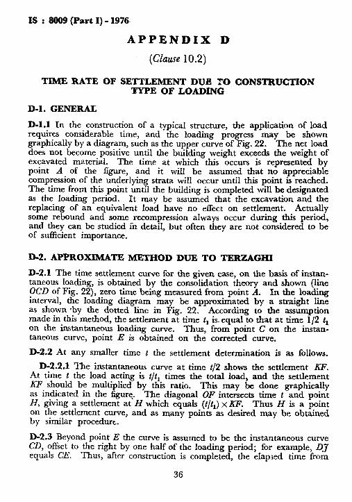
D-l.1 In the construction of a typical structure, the application of load requires considerable time, and the loading progress may be shown graphically by a diagram, such as the upper curve of Fig. 22. The net load does not become positive until the building weight exceeds the weight of excavated material. The time at which this occurs is represented by point A of the figure, and it will be assumed that no appreciable compression of the underlying strata will occur until this point is reached. The time from this point until the building is completed will be designated as the loading period. It may be assumed that the excavation and the replacing of an equivalent load have no effect on settlement. Actually some rebound and some recompression aiways occur during this period, and they can be studied in detail, but often they are not considered to be of sufficient importance.

D-2. APPROmTE MEJX-IOD DUE TO TERZAGHI

D-2.1 The time settlement curve for the given case, on the basis of instan- taneous loading, is obtained by the consolidation theory and shown (line OCD of Fig. 22), zero time being measured from point A. In the loading interval, the loading diagram may be approximated by a straight line as shown ‘by the dotted line in Fig. 22. According to the assumption made in this method, the settlement at time t, is equal to that at time l/2 t, on the instantaneous loading curve. Thus, from point C on the instan- taneous curve, point E is obtained on the corrected curve.

D-2.2 At any smaller time t the settlement determination is as follows.

D-2.2.1 The instantaneous curve at time t/2 shows the settlement KF. At time t the load acting is t/t1 times the total load, and the settlement KF should be multiplied by this ratio. This may be done graphically as indicated in the figure, The diagonal OF intersects time t and point H, giving a settlement at H which equals (t/Q x KF. Thus H is a point on the settlement curve, and as many points as desired may be obtained by similar procedure.

D-2.3 Beyond point E the curve is assumed to be the instantaneous curve CD, offset to the right by one half of the loading period; for example, 03 equals CE. Thus, after construction is completed, the elapsed time from

36

thl it

D”

D. do va in ch; ch; cot CO1

IN

Y load hown t load r;ht of :d by &able iched. mated td the tually eriod, to be

nstan- (line

‘ading t line tp tion l/2 t1 zstan-

llows.

t KF. :ment ucally point point :ained

curve :> DJ from

I 1

ASSUMED EFFECltVE LOADING PERIOD

L----CONSTRUCTION PERIOD ---d

$Al.4,N4A N EO U S

1

FIG. 22 TERZAGHI’S APPRCXIMATE METHOD

the start of loading until any given settlement is reached is greater than it would be under instantaneous loading by one half of the loading period.

D-3. GRAPHIGAL SOLUTION

D-3.1 An alternative graphical solution for construction type of loading, does not involve an approximation of the loading diagram with linear variation as in the previous method. In this method, the charts shown in Fig. 23A and 23B are used for this purpose. The small squares in the chart represent a given fraction of consolidation as noted in the particular chart. The value of each small square in Fig. 23B is only half of the corresponding value of Fig. 23A and hence the former may be used if the consolidation is less than 50 percent so that the accuracy of the final result

-

Y

_._ __-

IS : 8009 (Part I) - 1976

can be increased. The horizontal axis represents the time factor. The vertical axis is the load axis. Let the time load curve be as shown in Fig. 24. The time axis is first replaced by the time factor axis. Then, the consolidation at time 1, is determined as follows.

D-3.2 The load time factor curve is drawn on the chart as a mirror reflec- tion starting from the time factor l-, corresponding to time t,. It is to be noted that the mirror reflection is to be obtained by warping the time factor axis of the time load curve to suit the corresponding scale in the reflected part of the chart, as shown in Fig. 24. The number of squares under this curve multiplied by the value of each square is equal to the consolidation at time t,.

38

IS : 8009 (Part I) - 19’76

0 1 2 4 68 1

lo” rl;

2 5 67891

TIME FACTOR T

1*2 I*4 1.6 la8 2*i

238 Chart with value of each small square ;=@025%

FIG. 23 CHART FOR FINDING CONSOLIDATION DUE To CoNsTRucTIoN TYPE LOADING

39

0 l*O 2.0 2*5 3=0 TIME FACTOR 0 1-O 2*0 3.0 400 5*0 6.0 TIME IN YEARS

TIME LOAD CURVE

0 0.1 0.2 O-25 O-3 1-o

f IME FAC TOR

FIG. 24 USE OF C:o%oLATIoN CHART

40

AMENDMENT NO. 1 MAY 1981 TO

IS : 8009 ( Part I J-1976 CODE OF PRACTICE FOR CALCULATION OF SETTLEMENTS

OF FOUNDATIONS

PART I SHALLOW FOUNDATIONS SUBJECTED TO SYMMETRICAL STATIC VERTICAL LOADS

Corrigeatda

(Page 6, clause 3.0, line 5 ) - Substitute r C ’ for c c ‘.

( Page 15, clause 9.1.2, equation 2 ) - Substitute ‘ C’ for c c ‘.

( Page 22, Fig. 12, legend) - Substitute ‘ “52 ‘for _$z ’

( Page 32, clause B-3.2, last line ) - Substitute ’ r~ ’ for ‘ qz ‘.

Alterations

‘ IS :

(Page 7, c&se 3.0, symbol S1 ) - Delete along with its explanation.

( Page 12, clause 7.1, lint 2) - Substitute ~‘ IS: 1892-1979* ’ JGr 1892-1962* ‘.

( Page 12, foot-note with ‘ * ’ mark j - Substitute the following for . . ^ the existmg foot-note:

‘ *Code of practice for sub-surface investigations for foundation (jirst reoision). ’

15 clause 9.1.2 lines 2 and 3 ) - Substitute ‘ IS : 4968 ( Par>IT?Fl97f* ‘for ‘ IS : 4668 ( Part III )-1971* ‘.

(Page 15, foot-note with c * ’ mark ) - Substitute the following for the existing foot-note:

‘ *Method for subsurface sounding for soils : Part III Static cones penetration test (jirsf revision ) .’

( Page 16, clause 9.1.3 ) clause:

- Substitute the following for the existing

( 9.1.3 Method Based on Plate Load Test - Plate load test should be per- formed at the proposed foundation level and the settlemrnt of a square

c

plate under the design intensity of loading on the foundation estimated (see IS: 1888-1971” ). Then the total settlement of the proposed founda- tion is given by:

2 & = s C B(B +3Oj ____!L._-

’ B,(B+30) 1 NOTE - If the water tnbIe is at shallow depths or if it is expected that the water

tab!? for the foundations will be different from what is obtained at the time of the field !oad test, then, the efft-ct of water tablr on the bearing capacity of the founda- tions may be different from that for the load test. Therefore, the water table correction given in Rg. 9 may be suitably adopted for the load test and the founda- tions ‘.

( Page 16, clause 9.1.4, last sentence ) - Substitute the following for the existing sentence:

‘ If the water table is at a shallow depth, the settlement read from Fig. 9 shall be divided, by the correction factor w’ read from the inset in the same figure. ’

( Page 16, clause 9.2.2.1 )‘- Substitute the following for the existing clause:

‘ 9.2.2.1 For situations shown in Fig. 2 it may be assumed that:

Sr = 0, and

SC = Soecl

NOTE -To be exact, the settlement of the sand layers may also have to he added to the computed value of Sf . The designer has to use his discretion whether to add the settlement due to the sand layers or not.

The details of the computations of Soee depends upon the preIoading conditions. The details are given in 9.2.2.2 to 9.2.2.4.’

Addendum

( Pqe 7, clause 3.0 ) -Add the following symbols at appropriate places:

’ S,, = Settlement of test plate under a given load intensity per unit area, cm

B1, = Size of test plate, cm ’

AMENDMENT NO. 2 JULY 1990 TO

XS 8009 ( Part 1 ) : 1976 CODE OF PRACTICE FOR CALCULATION OF SETTLEMENTS OF

FOUNDATIONS

PART 1 SHALLOW FOUNDATIONS SUBJECTED TO SYMMETRICAL STATIC VERTICAL LOADS

[ Pa,ce 2X, clause B-1.3, expression ( R 2 ) 1 - Substitute the following tta- the existing matter:

!

/

I (BDC4:,)

Printed at Simco Printin Press, Delhi, India