IPOs, trade sales and liquidations: modelling venture

capital exits using survival analysis

Pierre Giot

Armin Schwienbacher∗

April 18, 2005

∗Pierre Giot is from Department of Business Administration & CEREFIM at University of Namur, Rempartde la Vierge, 8, 5000 Namur, Belgium, Phone: +32 (0) 81 724887, Email: pierre.giot@fundp.ac.be and isa research fellow at CORE, Universite Catholique de Louvain, Belgium. Armin Schwienbacher is from theUniversity of Amsterdam, Finance Group, Roetersstraat 11, 1018 WB Amsterdam, The Netherlands, Phone:+31 (0) 20 5257179, Email: a.schwienbacher@uva.nl.

IPOs, trade sales and liquidations: modelling venture capital exits using survival analysis

ABSTRACT

This paper examines the dynamics of exit options for US venture capital funds. Using

a detailed sample of more than 20,000 investment rounds, we analyze the time to ‘IPO’,

‘trade sale’ and ‘liquidation’ for 6,000 venture-backed firms. We model these exit times

using competing risks models, which allow for a joint analysis of exit type and exit timing

as well as their dynamic interplay. Biotech and internet firms have the fastest IPO exits.

Internet firms are also the fastest to liquidate, while biotech firms are however the slowest.

The hazard rate for IPOs are clearly non-monotonous with respect to time. As time flows,

venture capital-backed firms first exhibit an increased likelihood of exiting to an IPO.

However, after having reached a plateau, investments that have not yet exited have fewer

and fewer possibilities of IPO exits as time increases. This sharply contrasts with exit

options through a trade sale, where the hazard rate is less time-varying.

2

1. Introduction

The assessment of possible exit options is of paramount importance for venture capitalists

prior to their investments in new ventures. Indeed, not only are they concerned abouthow

they can cash out but alsohow longthey need to be involved in their portfolio companies

before cashing out. Besides the offer price, the exit decision therefore features two important

dimensions. First, the type of exit route (the most important ones being IPO, trade sale and

liquidation)1 and secondly the actual timing of the exit. The existing academic literature on

venture capital exits has shown that venture capitalists time their exits using stage financing

split into several rounds (e.g. Gompers, 1995, Bergemann and Hege, 1998). Besides the dis-

ciplinary action that this procedure exerts on venture capital-backed firms, this stage financing

also provides exit options to venture capitalists at all financing rounds. This allows the VCs

to time their exit. In addition to stage finance, several studies document the widespread use of

contractual arrangements that guarantee the venture capitalist explicit intervention rights, also

regarding exit issues (Gompers, 1997, Cumming, 2002, and Kaplan and Stromberg, 2003).

More generally, these rights allow the venture capitalist to force an exit. Thus, they can avoid

being locked into holding the shares for an extended period of time should a disagreement

with the entrepreneur occur. Moreover, the recent stock market developments witnessed over

the last few years highlight the dependence of venture capital investments on prevailing exit

conditions.

While IPO exits by VC funds have been researched quite extensively,2 a stock market list-

ing is however only one out of several ways to exit private equity investments. Interestingly,

the academic literature has not focused much on other types of exits such as trade sales and

liquidations. Nor do we know how these various exit routes interact as time flows. Moreover,

little is known about the effect of the recent internet bubble on the relative importance of com-

peting exit possibilities (especially trade sales compared to IPOs). In this paper, we consider

both dimensions (i.e. type and timing) of exit within a single framework of analysis. Thus, we

explore the full range of exit routes, i.e. not only IPOs, but also trades sales and liquidations.

This is particularly important when tackling the issue of ‘exit risk’ for venture capital invest-

1Note that we also use the word ‘trade sales’ for so-called acquisitions.2See, among others, Lerner (1994), Gompers (1995, 1996), Black and Gilson (1998), Cumming and Mac-

Intosh (2003), Cochrane (2005), Cumming (2002), Schwienbacher (2005), and Das, Jagannathan, and Sarin(2003).

2

ments as it requires jointly taking into account all potential exit routes. We also assess how

exit conditions evolve when firms move up the ladder of financing rounds and compare these

results with the prevailing conditions at the initial (first round) investment. This provides a

better picture of the dynamics of exit options for venture capital funds.

In the last part the paper, we also tackle the issue as to whether the geographical location

of the entrepreneurial firm affects the two dimensions of exit. For instance, does an investment

in the Silicon Valley facilitate VC funds exits more than a similar investment in Texas or on

Route 128?3 If it does, the firm’s cost of capital would be directly affected as VC funds would

require a lower cost from firms in more favorable regions. Hence, this would lead to important

implications for the clustering of entrepreneurial firms. Last, we examine how the internet

bubble affected the exit conditions of venture-backed companies. More specifically, we look

at whether investments made during the bubble period affected the times to exit and exit types

as compared to similar deals made outside this period. The internet bubble period was said

to be characterized by easy exits. Market conditions then changed dramatically in 2001 and

2002 as the NASDAQ and most stock indices crashed. Recent studies show that exit conditions

are highly cyclical and strongly depend on the current or foreseen state of stock markets as

well as other macro-economic factors (Lerner, 1994, Gompers and Lerner, 1998, Jeng and

Wells, 2000, Bottazzi and Da Rin, 2001, and Cumming, Fleming, and Schwienbacher, 2003).

Correspondingly, the exit from successful firms should have been easy. For unsuccessful

ventures this may be attributed to the desire by venture capitalists to pull the plug more quickly

and redirect their effort in new projects since they face a tradeoff between the number of

portfolio companies and the time spent with each companies (Kanniainen and Keuschnigg,

2003). Some industries may also have been more affected than others during the bubble

periods (Das, Jagannathan, and Sarin, 2003).4

Using a detailed sample of more than 20,000 investment rounds, we analyze the time to

exit through IPO, trade sale and liquidation for about 6,000 venture-backed firms. In the

framework of survival analysis, we characterize and model the times to exit using competing

risks models, which allow for a joint analysis of exit type and exit timing as well as their

dynamic interplay. To our knowledge, this is the first application of such statistical models

3On the difference between Silicon Valley and Route 128, see Aoki (1999), Saxenian (1994), and Hellmannand Perotti (2004).

4See Cassidy (2002) for a lively account of the internet bubble.

3

to venture capital investments.5 The strength of our approach lies in the rigorous statistical

modelling of exit times, and the possibility to fully parameterize the exit times with known

covariates (i.e. explicative variables known at the time the investment round took place). In

this framework, each type of exit exhibits its own dynamics and has its own dependence with

respect to variables such as the industry type of the firm, the size of the syndicate or the amount

of venture capital received. Quite importantly, the use of the generalized Gamma density dis-

tribution as the underlying statistical distribution in the competing risks models allows for

non-monotonous increasing/decreasing conditional probabilities of exits (also called hazard

functions). For example, this allows for increasing (as time goes by) IPO hazard rates dur-

ing the firstn years, and thereafter decreasing conditional probabilities of exit. Because the

dynamics of the times to exit depend on the selected explicative variables that pertain to the

status of the firm or the characteristics of the investment round, we can highlight the pattern

shown by firms that belong to a specified industry (e.g. internet firms vs biotech firms) or that

were funded during the internet bubble time period.

The empirical analysis delivers key results which can be summarized as follows. First,

biotech and internet firms have the fastest IPO exits. Internet firms are also the fastest to liq-

uidate, while biotech firms are however the slowest. Internet start-ups are quickly terminated

if they don’t achieve technological advancement fast enough. This effect is much less pro-

nounced for biotech firms. Second, regarding the shape of the conditional probability (hazard)

of IPO exit, a first sharply increasing hazard and then a slowly decreasing hazard are ob-

served. Thus, as time flows, venture capital-backed firms first exhibit an increased likelihood

of exiting to an IPO. However, after having reached a plateau, investments that have not yet

exited have fewer and fewer possibilities of IPO exits as time increases. This pattern is the

strongest for biotech and internet firms which tend to reach their plateau sooner than computer

or semiconductor firms. We interpret this as evidence that IPO candidates tend to be selected

relatively quickly. In contrast, if they do not achieve a public listing fast enough, their chances

of doing so quickly decrease.

For trade sales, hazard functions reach their maximum much later and tend to decrease

slowly thereafter. This is very much in line with the widespread notion that, in contrast to an

5Note that Gompers (1995) and Cumming and MacIntosh (2001) also use duration models, but these are notcompeting risks models.

4

IPO, a trade sale is a more universal exit channel, i.e. a type of exit available to many firms

and not only to the most successful startups (Lerner, 1994, Bascha and Walz, 2001, Cumming

and MacIntosh, 2001, Schwienbacher, 2004). Venture capitalists do a trade sale for highly

successful as well as less successful portfolio companies. Sometimes, venture capitalists even

choose a trade sale for unprofitable ventures but for which a larger corporation is keen on

acquiring the technology. The latter firm is thus ready to pay more than the liquidation value

of the venture. This leads to a greater heterogeneity in the type of venture capital-backed firms

doing a trade sale as compared to venture capital-backed firms going public.

Third, the geographical location of the entrepreneurial firm does not seem to impact the

dynamics of the IPO process. In contrast, trade sales are significantly more likely (i.e. the

hazard rate increases significantly) for firms based in California (Silicon Valley) and northeast

states (Route 128). Similarly, liquidations are less likely in these regions. Since these are also

the regions that feature the largest clustering of entrepreneurial firms and venture capitalists

(and all other important players involved in venture capital finance), this may suggest that such

a concentration facilitates the success of these firms as compared to firms in other US regions.

Fourth, the bubble period was an ‘easy money’ period where venture capitalists gave much

more money to firms, many of which did not offer outstanding growth potential as they tended

to liquidate much faster than in normal times. Moreover, the bubble period sped up the exit

of investments already in the pipeline, i.e. investments who had been initiated some time ago

and for which venture capitalists were eager to have a now accelerated exit. Fifth, the bubble

affected some industries more than others: the internet, computer and communication/media

industries were strongly affected as firms in those industries exhibited significantly smaller

exit times during the bubble.

Finally and as expected, later (expansion) stage investments exit to IPO more quickly than

expansion (early) stage investments. Since an early-stage project is typically less developed

than a project in the expansion stage and especially later stage, the time-to-exit for successful

projects decreases with the development of the project. In particular, it is the largest for

early stage and the shortest for later stage projects. Survival should therefore be greatest

for ventures with more developed projects. The size of the syndicate of VC funds affects both

dimensions of exit. Most interestingly, it accelerates exits through all routes. In early rounds,

investments with larger syndicates tend to be divested more quickly (i.e., faster IPOs, trade

5

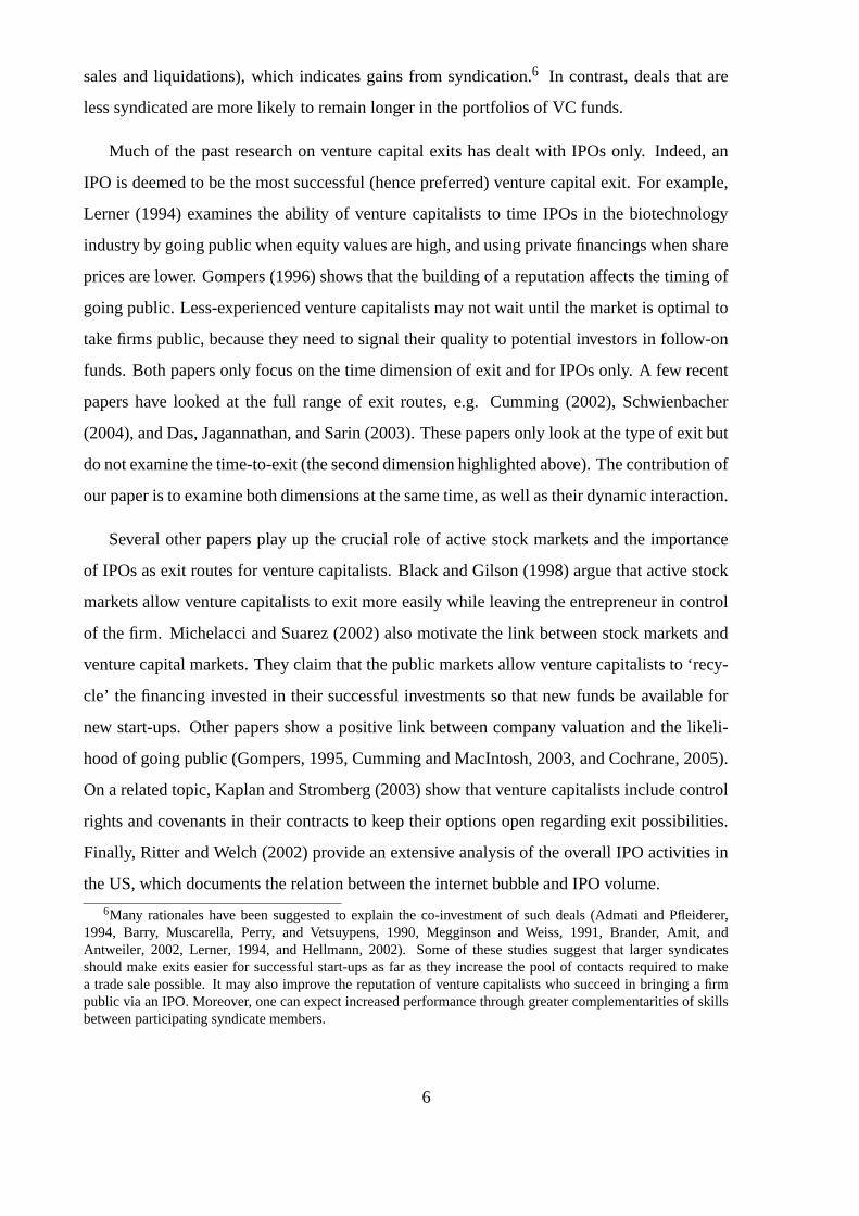
sales and liquidations), which indicates gains from syndication.6 In contrast, deals that are

less syndicated are more likely to remain longer in the portfolios of VC funds.

Much of the past research on venture capital exits has dealt with IPOs only. Indeed, an

IPO is deemed to be the most successful (hence preferred) venture capital exit. For example,

Lerner (1994) examines the ability of venture capitalists to time IPOs in the biotechnology

industry by going public when equity values are high, and using private financings when share

prices are lower. Gompers (1996) shows that the building of a reputation affects the timing of

going public. Less-experienced venture capitalists may not wait until the market is optimal to

take firms public, because they need to signal their quality to potential investors in follow-on

funds. Both papers only focus on the time dimension of exit and for IPOs only. A few recent

papers have looked at the full range of exit routes, e.g. Cumming (2002), Schwienbacher

(2004), and Das, Jagannathan, and Sarin (2003). These papers only look at the type of exit but

do not examine the time-to-exit (the second dimension highlighted above). The contribution of

our paper is to examine both dimensions at the same time, as well as their dynamic interaction.

Several other papers play up the crucial role of active stock markets and the importance

of IPOs as exit routes for venture capitalists. Black and Gilson (1998) argue that active stock

markets allow venture capitalists to exit more easily while leaving the entrepreneur in control

of the firm. Michelacci and Suarez (2002) also motivate the link between stock markets and

venture capital markets. They claim that the public markets allow venture capitalists to ‘recy-

cle’ the financing invested in their successful investments so that new funds be available for

new start-ups. Other papers show a positive link between company valuation and the likeli-

hood of going public (Gompers, 1995, Cumming and MacIntosh, 2003, and Cochrane, 2005).

On a related topic, Kaplan and Stromberg (2003) show that venture capitalists include control

rights and covenants in their contracts to keep their options open regarding exit possibilities.

Finally, Ritter and Welch (2002) provide an extensive analysis of the overall IPO activities in

the US, which documents the relation between the internet bubble and IPO volume.

6Many rationales have been suggested to explain the co-investment of such deals (Admati and Pfleiderer,1994, Barry, Muscarella, Perry, and Vetsuypens, 1990, Megginson and Weiss, 1991, Brander, Amit, andAntweiler, 2002, Lerner, 1994, and Hellmann, 2002). Some of these studies suggest that larger syndicatesshould make exits easier for successful start-ups as far as they increase the pool of contacts required to makea trade sale possible. It may also improve the reputation of venture capitalists who succeed in bringing a firmpublic via an IPO. Moreover, one can expect increased performance through greater complementarities of skillsbetween participating syndicate members.

6

The rest of the paper is structured as follows. After this introduction, we detail the data and

variables used in the analysis. We next present the competing risks model in Section 3. The

empirical application is split into 2 sections: Section 4 gives a detailed descriptive analysis,

while we present all the estimation results in Section 5. Finally, Section 6 concludes.

2. Data

The data used in this paper has been extracted from the VentureXpert database. Our database

is made up of successive records, each record pertaining to 1 investment round in a given

venture-backed firm. Note that whenever the firm was involved in more than one financing

round, we therefore have as many observations (per firm) as investment rounds, see below for

an example. Observations cover the period from 1/1/1980 to 6/23/2003 (date at which the data

has been collected). The data was pre-filtered to remove all records where the times-to-exit

(DURATION variable thereafter) are smaller than 14 days or larger than 20 years and we also

removed all records for which the amount of money received (AMOUNT variable) by the

firm is smaller than $10,000 or larger than $100,000,000. These observations are deemed to

be meaningless outliers for which the recorded values do not belong to a plausible range. This

pre-filtering leads us to discard very few records and gives us a sample made up of 22,042

investment rounds for 5,817 distinct venture-backed companies.7 More than 97% (90%) of

these screened firms were founded after 1970 (1980) and about 93% of the firms are estab-

lished in the USA (firms incorporated in California and Massachusetts add up to a substantial

proportion of the total US firms). Hence, our analysis mainly focuses on relatively recently

established US firms. The complete descriptive analysis is provided in Section 4. To charac-

terize the firms in our dataset and the stage financing they received from venture capitalists,

we use the following variables:

- On the industry type (dummy variable): INTERNET (internet industry), BIOTECH (biotech

industry), COMPUTER (computer industry), SEMIC (semiconductor industry), MEDI-

CAL (medical industry), COMMEDIA (communication and media industry) and OTH-

7Note that we get the same qualitative results and conclude similarly when using non-filtered data. It is how-ever well known that meaningless outliers can substantially affect the precision of the econometric estimations.We therefore focus on the filtered data.

7

ERIND (other industries than those listed above). These variables are equal to 1 (0) if

the given firm belongs (does not belong) to the specified industry.

- On the stage of development (dummy variable): EARLY (early stage financing), EXPAN-

SION (expansion stage), LATER (later stage), BUYACQ (buy/acquisition stage), OTH-

ERSTAGES (other stages than those listed above). Set to 1 (0) if the financing stage

matches (does not match) the description of the variable.

- On the type of exit (dummy variable): IPO (IPO exit), TRADESALE (trade sale exit), LIQ-

UID (liquidation exit). Set to 1 (0) if the firm exited (did not exit) according to the exit

specified by the variable. Note that many firms are characterized by IPO = 0, TRADE-

SALE = 0 and LIQUID = 0 as they are still ‘active’, i.e. venture capitalist have not yet

exited, or have exited via a fourth exit route. This latter route could include secondary

sales or management buyouts (MBO).8 This will yield right-censored durations in the

statistical analysis (see below for the DURATION variable and Section 3).9

- On the geographical location of the entrepreneurial firm (dummy variable): WEST (Cali-

fornia), NORTHEAST (Massachusetts, New York and Pennsylvania), SOUTH (Texas),

and MIDWEST (Illinois and Ohio). Set to 1 (0) if the location matches (does not match)

the description of the variable. For the classification of regions, we use the same defini-

tions of Lerner, Schoar, and Wong (2005).

- ROUND: ordinal round number of the investment. This indicates which financing round we

are dealing with.

- SYNDSIZE: syndicate size, i.e. number of venture capital firms that participated in that

financing round.

- AMOUNT: total amount of money received by the firm at the given round (in millions of

USD).

- BUBBLE: dummy variable equal to 1 if the investment was made during the bubble time

period from ranges from September 1, 1998 to April 30, 2000 (inclusive), and 0 other-

wise.8Because of the structure of the competing risks model used in the statistical analysis, the fact that we do not

model explicitly these other types of exit routes does not lead to any bias in our estimations for the IPO, tradesale and liquidation exits.

9Note that if a company had more than one financing round, we consider the exit type at the very end of thefinancing cycle (i.e. the exit route chosen at the end of the last round). In other words, for a given firm, thisvariable takes the same value for all financing rounds. See the examples given below.

8

- DURATION: number of days elapsed between the date at which the round began and the

exit date if there was an exit. If the firm has not yet exited, this variable gives the number

of days elapsed between the date at which the round began and the date of the analysis

(June 23rd, 2003).10 This variable is the main focus of our analysis as it characterizes

the ‘life’ of the investment since a given round.

We thus have a total of 18 explicative variables, although many of these variable are pure

dummy variables.11 The full statistical model is detailed in Section 3. As an illustration, Table

1 presents the data structure and definition of variables for two venture-backed firms that made

an IPO exit (Ask Jeeves and Brocade) and a third firm (InGenuity) that had not yet exited at

the date of the analysis (June 23rd, 2003). Although the analysis will be detailed in Sections 4

and 5, we can already see that Ask Jeeves, an internet firm, is characterized by a fast IPO exit

(DURATION = 303 days since round 1, which was an early stage round). Besides these 18

variables, we also define a secondary variable, AMOUNTIND, for the total amount of money

received by the firm (in millions of USD) in excess of the average amount of money received

by firms in that industry (at the given round). This variable is used later in the analysis.

3. Survival analysis and competing risks models

As briefly discussed in the introduction, our statistical analysis relies on survival analysis and

competing risks models. Competing risks models are powerful statistical models tailored to

model durations (also called time to failure) that end with multiple exits (also called multiple

type of failure). They originate from the engineering sciences and have been extensively

used in the medical sciences and in empirical studies of labor markets. In the first case, the

duration (or time to exit in the venture capital terminology used above) is typically the number

of days elapsed between the patient taking the given medicine and the possible failure (full

recovery or death by several distinct causes of the patient for example). In the second case,

the duration could be the length of time until an unemployed individual gets a job or quits

searching. Recently competing risks models have also been used in the modelling of high-

10This is characterized as a right-censored duration in the terminology of survival analysis. See Section 3.11Note that to avoid multicollinearity problems in the statistical analysis of Section 5, we do not include a

constant and we have to drop one of the dummy variables (as the industry type and stage of development typevariables sum to 1 separately): we do not include the OTHESTAGES dummy variable.

9

frequency stock market transaction data, where the duration is the time between a given price

change and the exits are an increase or decrease in the stock price (Bauwens and Giot, 2003).

In this section, we first detail a simple two-state competing risks model and then show how

we plan to use a multi-state competing risks model in the venture capital exits framework.

Additional information on survival analysis and/or competing risks models can be found in

Crowder (2001), Kalbfleisch and Prentice (2002) and Lee and Wang (2003).

3.1. A simple competing risks model

The next sub-section presents the competing risks model used in the empirical analysis of

Section 5. We however first present a simple competing risks model with 2 exits to illustrate

the general methodology. Let us consider a set of investments characterized by their durations

(i.e. times until exit) and their exit types. In this introductory example, we assume that there

are two exit possibilities (success and failure) and that the durations are not right censored.12

We thus have a set of pairs(xi ,yi), wherexi is the duration of the investment andyi is a

variable indicating the exit type. In this simplified example, there are only two possible exits

characterized by mutually exclusive end states:yi = 1 (success) oryi = −1 (failure). For

simplicity, let us assume that the hazard function is constant, which is equivalent to assume

an exponential distribution forxi .13 The idea of the competing risks model is to let the hazard

vary with the end state, in this case to have two hazards sinceyi is binary. Thus we defineλs

(respectivelyλ f ) as the hazard of durationxi when the end state isyi = 1 (respectively -1). In

most competing risks model, the hazards are made dependent on a set of covariates, which can

thus be viewed as explicative variables which speed up/slow down the exits. For example, the

exponential formλs = eβs,0+βs,1X1+...+βs,kXk (and correspondinglyλ f = eβ f ,0+β f ,1X1+...+β f ,kXk),

whereX1,. . . ,Xk are the covariates, is widely used to ensure the positivity of the hazards. As

in classical survival analysis, coefficientsβs,1,. . . ,βs,k,β f ,1,. . . ,β f ,k then allow an immediate

assessment of the influence of the explicative variables on the exits. At the end of duration

xi , either stateyi = 1 (success) or stateyi = −1 (failure) is realized. In the framework of a

12In competing risks models, durations are said to be right-censored if the corresponding individual or firm atrisk has not yet exited at the time of the analysis. Right-censoring is discussed below.

13In survival analysis, the hazard function gives at all times the conditional instantaneous probability of exitgiven that the subject at risk has not yet exited at that time. For example, in a medical science context, the hazardof death by heart attack at timet for a patient is the instantaneous probability of dying of a heart attack at timetgiven that the patient is still alive ‘just’ before timet.

10

competing risks model, the duration corresponding to the state that is not realized is truncated,

since the observed duration is the minimum of two possible durations: the one which would

realize ifyi = 1, and the one which would realize ifyi = −1.14 This implies that the realized

state will contribute to the likelihood function via its density function, while the truncated state

contributes to the likelihood function via its survivor function.15

3.2. A competing risks model for venture capital exits

The competing risks model detailed in the previous sub-section can be used to model the exit

times and types of exit of venture capital-backed investments provided that:

- we allow for multiple exits (IPO, trade sale and liquidation);

- we allow for right-censoring as many investments had not yet exited at the time of the

analysis (i.e. they were still categorized as ‘active’ investments by the venture capitalist);

- we allow for competing hazards that depend on a set of covariates (type of industry for the

firm, amount of capital given to the firm, size of syndicate,. . . ) that are known at the

time of the investment;

- we estimate the competing risks models for a given round. This stems from the fact that a

duration is defined herein as the time elapsed between the actual round date when the

firm received the funding from the venture capitalist and the time of the analysis (June

23rd, 2003);

14As indicated in Lee and Wang (2003): “This is perhaps the most important concept in competing risksanalysis. It is because the basic assumption for a competing risks model is that the occurrence of one type ofevent removes the person from risk of all other types of events and the person will no longer contribute to thesuccessive risk set.

15Assuming independence (conditionally on the past state) between the durations ending at statesyi = 1 andyi =−1, the joint ‘density’ of durationxi and stateyi in our simplified examples is then equal to

f (xi ,yi) =(λs

)I+i e−λsxi(λ f

)I−i e−λ f xi . (1)

where

I+i =

{1 if yi = 10 if yi =−1,

(2)

I−i = 1− I+i . (3)

For example, if stateyi = 1 is observed (I+i = 1 andI−i = 0), xi contributes to the likelihood function via the

density functionλse−λsxi and via the survivor functione−λ f xi . Details regarding the construction of likelihoodfunctions of competing risks models are available in Kalbfleisch and Prentice (2002).

11

- we allow for possible non-monotonously increasing or decreasing hazards, i.e. use den-

sity distributions such as the generalized Gamma density distribution for example. The

choice of the ‘right’ density distribution can be tricky. Monotonously increasing or

decreasing hazard functions are the simplest to use but imply that, as time flows, the

likelihood of exiting gets either larger and larger or smaller and smaller. In our context,

we could have a likelihood of instantaneous IPO exit that first gets larger and larger as

the firm gets the funding, but then decreases once the firm does not deliver good results.

After many trials and with the benefit of hindsight, we settle for the generalized Gamma

distribution, which is one of the most flexible density distributions available for survival

analysis studies.

In the empirical analysis of Section 5, we use the generalized Gamma density distribution

as pre-programmed in Stata. More specifically, the density distribution is specified as:

f (t,κ,σ,µ) =γγ

σ t√γΓ(γ)

e(z√γ−u) (4)

if κ 6= 0, and

f (t,κ,σ,µ) =1

σ t√

2πe(−z2/2) (5)

if κ = 0, whereγ = |κ|−2, z= sign(κ)(ln(t)−µ)/σ, u= γe(|κ|z). The dependence with respect

to the covariates is introduced throughµj = Xj β, where j is the observations’ index. In the

venture capital framework of this study (IPO, trade sale and liquidation exits) and if all 18

explicative variables detailed in Section 2 are included in the model, this translates into 3

specifications forµj as we have 3 mutually exclusive exit possibilities:16

µj,IPO = β1,IPOINTERNETj +β2,IPOBIOTECHj + . . .+β18,IPOBUYACQ, (6)

µj,TS= β1,TSINTERNETj +β2,TSBIOTECHj + . . .+β18,TSBUYACQ (7)

16Note that in practice more than 3 exit types are observed. This is also the case in our sample. We focushowever on the IPO, trade sale and liquidation exits as these are the most important exists and are the real focusof our analysis. Because of the multiplicative nature of the likelihood function for competing risks models (seeEquation (1)), not modelling explicitly the other (few) types of exits does not lead to any bias.

12

and

µj,LIQ = β1,LIQINTERNETj +β2,LIQBIOTECHj + . . .+β18,LIQBUYACQ. (8)

In these specifications, theκ andσ parameters determine the general shape of the hazard

function (monotonously increasing or decreasing, or more generally non-monotonous, as time

increases) while theβ parameters determine the ‘time acceleration’. Thej index refers to the

available observations per round. A significantly negative value for anyβ parameter implies

that an increase in the corresponding variable leads to a significantly faster exit. For example,

a significantly negativeβ8,IPO (the coefficient of the SYNDSIZE variable in the specification

of the IPO exit) would mean that, as the size of the syndicate grows, the time-to-exit for an

IPO gets shorter. Note that, for dummy variables, exponentiated coefficients (i.e.eβ1,IPO for

example) have an easy interpretation as time ratios. These time ratios can then be directly

compared with each other, yielding relative time ratios. The latter are very easy to interpret as

a relative time ratio indicates how fast/slowly the change of category impacts the (conditional)

exit probability. For example, the relative time ratio (for the IPO exit) of the internet industry

with respect to the biotech industry is equal toeβ1,IPO/eβ2,IPO.

4. Descriptive analysis

In this section, we provide a descriptive analysis of our dataset. Estimation results for the

competing risks model are given in the next section. While Table 2 provides the frequency of

exit routes for different types of investment stages, Table 3 gives a breakdown of key statistics

by investment rounds, industries and stages of development. Finally, Table 4 gives information

on the industry type and stages of development during the bubble period and outside that

period.

Table 2 shows that the proportion of exit types is quite similar across financing stages,

except from the fact that there is a slight increase in trade sales with the increasing stage of

development (and the decreasing likelihood of IPOs). In both panels, the ratio of trade sales

13

over IPOs therefore tends to increase. Furthermore, this ratio is always greater than 1. For

instance, there are about 50% more trade sales than IPOs for early-stage investments.

A breakdown of AMOUNT and SYNDSIZE by round number (Panel A of Table 3, shown

for up to round 5) shows that the AMOUNT variable increases steadily when going from

round 1 to round 4. From round 3 onwards, it however stabilizes around $9 million. The fact

that firms receive a much lower amount of money in their first round of financing is consistent

with the literature: venture capitalists do not want to commit too many funds at the start of the

venture capital process. Note although that there is a great standard deviation in all rounds.

The SYNDSIZE variable also seems to be lower for the first rounds. For all types of exits,

the duration decreases as the number of rounds increases, which is to be expected and is in

line with the literature that conjectures a reduction in duration as the project is developed. For

example (IPO exit), the mean duration goes from 1,620 days to 925 days as the representative

firm goes from round 1 to round 5 (for trade sales, it decreases from 2,059 days to 1,506 days;

for liquidations, it decreases to 981 days from 1,554 days). Again, there is a variability in the

means for all the exit routes.

The breakdown of firms across industries (Panel B of Table 3) shows that internet and com-

puter companies attract the substantial part of the venture capital invested, while biotech com-

panies are much less represented (in absolute number). Similarly, a breakdown of AMOUNT

and SYNDSIZE by type of industry (Panel B of Table 3) shows that the average internet firm

was given much more money (around $12.9 million) that the other types of firms. Commu-

nication/media firms rank second (mean of $9.5 million), while the other firms received on

average around $6-9 millions. The mean of SYNDSIZE does not really change across indus-

try types. Focusing on IPO exits only, it becomes obvious that internet firms had the fastest

exit, with a mean of 670 days. Firms in the other industries needed much more time, the

slowest being the semiconductor firms (mean duration of 1,725 days). When focusing on liq-

uidations, it is also true that internet firms had the fastest exits (the representative internet firm

exhibits a mean duration to liquidation of around 721 days).

Looking at the pattern of AMOUNT and SYNDSIZE for the different financing stages

(Panel C of Table 3), we see that buyouts/acquisitions provide the largest mean amount (around

$14 million) and involve on average 3 venture capital firms. In contrast, early stage invest-

ments are characterized by an average amount of $5.1 million and an average of 3.5 venture

14

capital firms. For IPO exits, a breakdown of DURATION per financing stage yields a mean

of 1,581 days (early stage), and decreases as we go to the expansion and later stages. Further-

more, we observe similar patterns for trade sale and liquidation.

The BUBBLE variable characterizes investments that took place during the so-called bub-

ble time period for the NASDAQ. Table 4 provides summary statistics for investments during

the internet bubble (BUBBLE = 1) as well as in ‘normal times’ (BUBBLE = 0). During the

bubble period, internet type investments made up 39.2% of all investments, the computer in-

dustry being number 2 with 23.1%. Note that biotech investments made up only 4.1% of

all investments during the bubble time period (against 7.2% in ‘normal times’). There are

however no sharp differences between the stages of financing (early/expansion/later stages)

regarding the bubble and normal time periods. Early and expansion (later) stage investments

are somewhat less (more) frequent during bubble times. In contrast, there is a sharp difference

in the amount of money given to firms when in normal or bubble times. Indeed the mean

amount increases from $6.6 million to $13.4 million!17 Finally, the mean duration to exit

(irrespective of the type) is only equal to 344 days in bubble times, while it is equal to 1,328

days in normal times. In this case the difference is also highly significant.

As for the geographical location (bottom of Table 4), about half of the entrepreneurial firms

in our sample are located in California (WEST). The next largest region is NORTHEAST.

About one third of the investments in our sample are from other regions, which also include

all those outside the USA. This contrasts with the location of VC funds that are much more

concentrated in the West and Northeast regions. Indeed, these latter two regions account for

almost 80% of the VC funds located in the USA (Lerner, Schoar, and Wong, 2005).

5. Estimation results

The descriptive analysis of the previous section provided information on the dataset and on

the exit characteristics. In this section we estimate the competing risks model to fully describe

and analyze the exit process. We characterize extensively the estimation results for rounds 1

17Statistical tests clearly reject the null hypothesis that the two means are equal.

15

and 2, but then lump together the comments for rounds larger than 2 as these estimations do

not bring a lot of additional interesting results.

For all types of exits, we first estimate the model with all explanatory variables save for

the geographical location variables included as covariates. We use the generalized Gamma

density function as the distribution for the underlying error term.18 In a later step, we will

assess the impact of the geographical location by estimating an enhanced model that features

18 variables as covariates. We also allow for heterogeneity in our model.19 Allowing for het-

erogeneity leads to somewhat less efficient estimators when dealing with small datasets. We

however have a very large dataset and the minor loss of efficiency is irrelevant here. Note that

we conclude similarly (from a qualitative point of view) with and without the frailty estimation

option. When dealing with venture capital data, there is a strong case for suspecting that there

is heterogeneity in the data. Indeed the quantitative information provided in the database is

only part of the picture as the important ‘qualitative’ information (e.g. quality of the product

developed by the firm, its degree of innovation, the current technological trends,. . . ) about the

venture-backed firm is not included. We present the estimation results for the first and second

rounds in Table 6 and for the third and fourth rounds in Table 7. Note that we analyze the

residuals of the models after each estimation. As suggested by the literature on survival anal-

ysis (Engle and Russell, 1998, Kalbfleisch and Prentice, 2002), we focus on the generalized

Cox-Snell residuals (Cox and Snell, 1968): if the model fits the data well, then these residuals

should be exponentially distributed. This can be checked by plotting their cumulative hazard

function, along with the benchmark line with slope equal to 1. Anticipating on the estimation

results given below, we can already claim that the fit of the models is very good. As examples,

we provide such plots in Figures 5 and 6 (IPO, trade sale and liquidation exits, rounds 1 and

2).20

18We avoid multicollinearity problems by not including the constant and the OTHERSTAGES dummy vari-able.

19We do this by estimating the model with the ‘frailty’ option provided in Stata. Details are available inKalbfleisch and Prentice (2002) and in the “Survival analysis and epidemiological tables” Stata reference guide.

20Note that the somewhat ‘erratic’ line segments at the top right corner of some of the graphs refer to a coupleof extreme residuals (outliers), while the hundreds of residuals cluster around the straight line with slope equalto 1.

16

5.1. Round 1 (5,817 observations)

5.1.1. Exit to IPO

All coefficients (except for the BUYACQ and SYNDSIZE variables) are significant at the

5% level and have the expected sign. In particular, later stage investments exit more quickly

than expansion stage investments. This is also the case for expansion and later stage in-

vestments with respect to early stage investments, which is in accordance with the literature

review provided in the Introduction. This is confirmed by Wald statistical tests, according to

which the null hypotheses coef(EARLY)> coef(EXPANSION) and coef(EXPANSION)>

coef(LATER) are not rejected individually. From a statistical point of view, larger syndicate

sizes somewhat increase the hazard for IPOs, and thus decrease exit times, as the SYNDSIZE

coefficient is significant at the 6% level. This coefficient is however very small (-0.026) and

therefore an increase in the syndicate size does not really impact the timing of the exit in a

meaningful way. For example, an increase of the syndicate size from 4 to 8 implies a rel-

ative time ratio of onlye−0.026·8/e−0.026·4 = 0.9. In line with the literature review on faster

project realization, larger committed amounts also decrease exit times (significantly negative

AMOUNT coefficient). This is also the case for the secondary variable AMOUNTIND, i.e.

the amount of funds received in excess of the average firm in the same industry (note that

because of collinearity problems, we estimate the models separately with the AMOUNT and

AMOUNTIND variables).

The time ratio representation allows an easy comparison across industry classifications.

Biotech firms have the fastest exits and are followed by internet firms. With respect to these

firms, computer firms exhibit a relative time ratio of almost 1.5 (computed ase8.886/e8.476)

while the other industries are in-between (not taking into account the ‘other industries’ cate-

gory). Wald statistical tests indicate that the null hypothesis coef(INTERNET)= coef(BIOTECH)

cannot be rejected, while the coefficients of the other industries are individually significantly

different from the coefficients of the INTERNET and BIOTECH industries (for example the

null hypothesis coef(INTERNET)= coef(COMPUTER) is rejected).

The model rejects the null hypothesis of monotonously increasing or decreasing hazard.

Hence, the generalized Gamma cannot be simplified into the Weibull density distribution for

17

example. This is shown in Figure 1, where we plot the estimated hazard function for the first

4 industry classifications for a typical venture capital-backed firm that would receive (at the

early stage and outside the bubble time frame) a $10 million funding provided by a syndicate

of 4 venture capitalists, i.e. the covariates are fixed such as SYNDSIZE = 4, AMOUNT = 10,

BUBBLE = 0 and EARLY = 1.21 Regarding the shape of the hazard functions, one has first a

sharply increasing hazard (to about 1,000 - 1,500 days) and then a slowly decreasing hazard.

Thus, as time flows, venture capital-backed firms first exhibit an increased likelihood of exiting

to an IPO. However, after having reached a plateau (around 1,000 - 1,500 days of existence,

i.e. 2.75 - 4.0 years), investments that have not yet exited have fewer and fewer possibilities

of exits as time increases. This suggests that venture capitalists should not hesitate to ‘pull the

plug’ after a given number of years, rather than stick with potentially non-performing firms.22

This pattern is stronger for biotech and internet firms which tend to reach their plateau sooner

than computer or semiconductor firms (around 5 years (1,800 days) for these latter firms,

around 3.3 years (1,200 days) for the former). In the top panel of Figure 4 we plot the hazard

functions for an internet firm and the three financing stages, with SYNDSIZE = 4, AMOUNT

= 10, BUBBLE = 0. As expected, the maximum of the hazard functions shifts left as we

go from early to expansion and finally later stage financing. We then repeat the exercise for a

biotech and computer firm, and the results are given in the middle and bottom panels of Figure

4. Quite surprisingly, the BUBBLE coefficient is significantly positive, which leads to a time

ratio greater than 1: investments made during the bubble period did not lead to faster IPO exits

(we delve more deeply on this issue below, as this coefficient gets significantly negative for

rounds larger than 2).

5.1.2. Exit to trade sale

Estimation results are somewhat similar to those presented above for the exit to IPO, although

there are some differences. The coefficients for the AMOUNT and BUBBLE variables are no

longer significant while the coefficient for the SYNDSIZE variable is now highly significant.

The latter is in line with the idea that a larger syndicate increases the pool of corporate contacts

21To ensure a good readability of the graphs, we do not plot all 7 types of industries on the same graph. Fullpage color graphs for all industries are available on request.

22Note that this is similar to what is observed in the labor market regarding individuals seeking jobs. Indi-viduals who have been searching jobs for extended periods of time often have less and less chances of actuallygetting a job as time goes by.

18

required to find a buyer and thus do a trade sale. The relative time ratios between the different

industries are not as dispersed and belong to a tighter range. The classification is also different

as the internet, computer and communication/media firms have the fastest exit to a trade sale.

The plots of hazard functions in the middle panel of Figure 1 tell the same story (same covari-

ates as for the first figure of preceding sub-section). Note that in this case all hazard functions

reach their maximum much later (around 2,500 - 4,000 days, i.e. 6.8 - 11 years) and decrease

much more slowly thereafter. A comparison of hazard functions for exits to IPO and trade

sale suggests that venture capital-backed firms first aim for an IPO exit and then consider (or

are forced to consider) trade sale exits as their second choice. It also provides support for the

notion that candidates for a trade sale are less homogeneous than those for an IPO.

5.1.3. Exit to liquidation

There are some marked differences with respect to the successful exits (IPO and trade sale).

First the coefficients for the EARLY, EXPANSION, LATER and BUYACQ variables are quite

close and it is no longer true that coef(LATER)< coef(EXPANSION) and coef(EXPANSION)

< coef(EARLY): the timing of the stage does not seem to hint at a faster/slower liquidation

of the firm. In this case, the BUBBLE coefficient is strongly negative (with a time ratio of

e−0.704 = 0.49), which suggests that firms that received venture capital money during bubble

times have a much larger probability of quick liquidation. In Section 4 we showed that the

amount of money raised (per funded firm) during bubble times was much larger than during

normal times. This suggests that the bubble period was an ‘easy money’ period where venture

capitalists gave much more money to firms, many of which did not offer outstanding growth

potential as they tended to liquidate much faster than in normal times. The relative time ratio

of internet firms with respect to the other firms is also striking as it is between 1/3 and 1/4!

This is clearly shown in the bottom panel of Figure 1 (same covariates as before) as there

is a clear gap between the hazard functions of internet related firms and the other types of

firms. Note also that the hazard function for internet firms quickly reaches its plateau (around

1,200 days) and strongly decreases thereafter. In contrast, biotech firms are the slowest to

liquidate (largest relative time ratio, slowly increasing hazard function and delayed plateau).

Lerner (1994) notes that “biotechnology firms [. . . ] mature slowly and do not incur large

up-front costs in building manufacturing facilities”, which could explain why (in conjunction

19

with the often lengthy Food and Drug Administration (FDA) approval process) these firms do

not tend to liquidate quickly. In contrast, internet firms have been known to be gobbling up

cash, which justifies their quick demise if they did not succeed in meeting their financial goals

within a limited time frame.

These estimation results also concur with the descriptive analysis given in Table 5. In this

table, we present the number and type of exit for first round investments made during and

outside the bubble period. A look at the left (bubble period) and right (outside the bubble

period) parts of that table reveals that liquidations occurred much more frequently during

the bubble period. While all industry sectors exhibit approximately the same pattern, results

for the internet sector are particularly impressive as both periods (i.e. inside and outside the

bubble period) are characterized by a large number of funded firms (164 vs 220). For some

of the other industry sectors (biotech and medical for example), results are more difficult to

interpret as few firms received first round financing during the internet bubble.

5.2. Round 2 (4,691 observations)

Because of the many similarities with the results of the first round, we highlight more partic-

ularly the results specific to round 2. Regarding the IPO exit, the results are similar to those

presented for the first round, although many coefficients are no longer significant (they still

have the expected sign though). Biotech and internet firms still have the lowest relative time

ratios, but the internet firms are much closer to the other firms than in round 1. Biotech firms

still exhibit an impressive halved time ratio with respect to most of the other firms. This is also

shown in Figure 2, where we plot the estimated hazard function for the first 4 industry clas-

sifications with SYNDSIZE = 4, AMOUNT = 10, BUBBLE = 0 and EARLY = 1. Note that

the hazard functions reach their maxima much earlier than for round 1 (around 700 days for

biotech firms, around 900 - 1,200 days for the other firms). This is of course consistent with

the fact that we now deal with the second financing round, which should thus be much closer to

the IPO than the first round. Again the general shape is decisively first sharply increasing and

then slowly decreasing as time goes by. This type of pattern is particulary striking for biotech

firms. For exits to trade sales, results are very close to those given above for the first round:

the relative time ratios are much less dispersed and the hazard functions reach their maxima

20

much later than for an IPO exit (around 2,000 days). Finally, for liquidation exits, results are

also similar to those for the first round. In this case, the BUBBLE coefficient is again sharply

negative, with a time ratio of 0.47 (i.e.e−0.755). As for the first round, internet (biotech) firms

have the lowest (largest) time ratio. See also the hazard functions plotted in the bottom panel

of Figure 2. Note however that coef(LATER)< coef(EXPANSION)< coef(EARLY), but the

coefficients are not significant.

5.3. Round 3 and above

Focusing on the results specific to these rounds we see that, for all rounds and all exits, the

BUBBLE coefficient is now negative. The hazard functions (plotted in Figure 3) reach their

maxima within a couple of months, and then sharply decrease. Round 3 biotech investments

are particularly impressive.

5.4. All rounds: summary of main results

The empirical results given above can be summarized as follows. Later stage investments exit

to IPO more quickly than expansion stage investments. This is also the case for expansion

and later stage investments with respect to early stage investments. The industry type clearly

matters as biotech and internet firms have the fastest IPO exits. Internet firms are the fastest to

liquidate, while biotech firms are the slowest. Regarding trade sale exits, internet, computer

and communication/media firms have the fastest exits. The model generally rejects the null

hypothesis of monotonously increasing or decreasing hazards for all specifications. Regarding

the shape of the hazard functions (exit to IPO), one has first a sharply increasing hazard and

then a slowly decreasing hazard. Thus, as time flows, venture capital-backed firms first exhibit

an increased likelihood of exiting to an IPO. However, after having reached a plateau (around

1,000 - 1,500 days of existence), investments that have not yet exited have fewer and fewer

possibilities of IPO exits as time increases. This pattern is stronger for biotech and internet

firms which tend to reach their plateau sooner than computer or semiconductor firms (around

1,800 days for these latter firms, around 1,200 days for the former). This motivates the ‘limited

partnership’ structure of VC firms where VC investment funds automatically dissolve after a

21

given number of years (rather than sticking with ongoing investments). The bubble period

was an ‘easy money’ period as venture capital-backed firms were awash with funds but many

of these firms tended to liquidate much faster than in normal times. Furthermore the bubble

period led to significantly decreased exit times for investments made at round 3 or above.

This suggests that the bubble period sped up the exit of investments already in the pipeline,

i.e. investments who had been initiated some time ago and for which venture capitalists were

eager to have a now accelerated exit. Broadly speaking, we conclude similarly for all rounds.

Of course, as the round number increases, hazard functions tend to shift leftwards, as one get

closer and closer to the exit (particulary true for the IPO exit).

5.5. The internet bubble and the industry type

These estimation results suggest that exits were sped up during the internet bubble. Indeed the

evidence is conclusive for the IPO and trade sale exits (starting at round 3) and strongly con-

clusive for the liquidation exit (all rounds). It can however be argued that the internet bubble

has affected some firms more than others. We conjecture that the bubble has sped up the exits

for specific industries, while it has hardly affected others.23 This hypothesis can be tested with

our dataset and within the framework of the competing risks model. To do this, we remove the

INTERNET dummy variable from the model and include 7 additional industry type dummy

variables. These new industry type variables (INTERNETB, BIOTECH B, COMPUTERB,

SEMIC B, MEDICAL B, COMMEDIA B and OTHERINDB) are dummy variables that are

equal to 1 when the firm is in the given industry AND the given financing round took place

during the bubble. We then estimate the competing risks model with the 13+7 variables hence

defined. Estimation results are given in Table 8. Note that we only report results for the 7 new

internet bubble related variables as the estimated coefficients of the 13 previous variables do

not really change. A bird’s eye view of that table ascertains that 3 of the 7 industries were

strongly affected by the bubble: the internet, computer and communication/media industries.

For these industries, the bubble sped up the liquidations (all rounds) and the IPOs (round 3

and above). In contrast, the bubble did not really impact the other industries as the corre-

23Of course the name ‘internet bubble’ by itself indicates that the worst excesses of the stock market bubblewitnessed at the end of the 1990s were to be found in the internet industry.

22

sponding dummy coefficients in Table 8 are not significant. These results strongly support the

hypothesis that the bubble did not have an evenly impact on all venture capital financings.

5.6. The impact of the geographical location

Does the geographical location of the entrepreneurial firm affect the exit dynamics? To tackle

this issue, we estimate an enhanced model that features all 18 explicative variables, i.e. the 14

original variables and the 4 geographical location dummy variables (WEST, NORTHEAST,

SOUTH and MIDWEST). Estimation results for the first and second rounds are reported in

Table 9. Regarding the IPO exit, there are few significative differences between the US re-

gions, although firms in the Midwest area seem to exit much less frequently. In contrast, trade

sale and liquidation exits are sharply different for, on the one hand, West and Northeast firms

and, on the other hand, South and Midwest firms. Indeed, firms face much easier trade sale

exits in the West and Northeast regions than for the other two regions. As far as liquidations

are concerned, firms in the South and Midwest regions tend to liquidate much faster than firms

in the West and Northeast. The difference is sharply significant, as shown by the time ratios

which are almost halved when switching from a West firm to a Midwest firm (e.g. at round

2, the time ratio would bee−0.707/e−0.057 = 0.522). To illustrate, Figure 7 presents the IPO,

trade sale and liquidation hazard rates for an average firm hypothetically situated in the four

US regions.

5.7. A brief discussion of related results

The analysis based on competing hazard models has provided a number of interesting results

regarding the dynamics of the exit pattern for venture capital-backed firms. Some of these

results are strongly related to previously reported findings in the literature on venture capital

and exit strategies by venture capital-backed firms. We briefly discuss these here and stress

the contribution of our analysis to this recent strand of the literature.

Exits occurred much more frequently during hot issue markets (here, the internet bubble

is in line with observations provided by Lerner (1994)), which indicates that venture capital

funds are able to time their IPO exits earlier when stock market valuations are highest (see

23

also the survey in Jenkinson and Ljungqvist, 2001). While the study of Lerner (1994) only

dealt with biotech firms, our analysis indicates that this also holds during the internet bubble

period for firms in the internet, computers, communications and media sectors. Interestingly,

these same industry sectors also had significantly quicker liquidations during the time of the

internet bubble period. This highlights the fact that venture capitalists incurred a large risk

when investing in companies that potentially had a great upside potential but also exhibited a

high risk of failure. Gompers (1995) provides evidence that the degree of asymmetric infor-

mation has a significant impact on the time-to-exit. This implies that early-stage investments

require a longer lasting involvement of venture capital funds than later-stage investments, since

asymmetric information decreases along with the reduction of technological risk. Our paper

provides further evidence in line with this rationale.

Cumming and MacIntosh (2001) find that exits occur more quickly for early stages of de-

velopment, which they interpret as the result of a selection process to sort out the bad from the

good projects. Our study provides a somewhat different picture. While exits from later-stage

investment are quicker than for early-stage investments (irrespective of the type of exit route)

at the time of deal initiation, the results are mixed for later-round investments. Finally, Das,

Jagannathan, and Sarin (2003) look at cumulative probabilities of exits. Among other things,

they find that the likelihood of a trade sale increases with the stage of development (“this may

be because many early-staged firms that were unable to make it to the IPO stage settled instead

for a buyout”). They further show that successful companies in biotech and medical sectors

exit more frequently. Our study goes a step further and looks at the time dimension of the

exit process, how the exit probabilities evolve over time and how the dynamics of the exit pro-

cess if affected by the actual outcome (IPO, trade sale or liquidation). In particular, the most

striking feature is the difference between trade sales and IPOs (the main exit routes). While

probabilities do not change that much in the first case, the probability of doing an IPO exhibits

a strong, inverse U-shaped pattern; it increases very quickly and again decreases sharply right

after it peaked. Successful companies that could not go public sufficiently quickly have to rely

on other exit routes like trade sales.

24

6. Conclusion and outlook

For venture capitalists, the decision to exit has two main dimensions, the type and the timing

of the exit. This paper has examined both dimensions of exit simultaneously in the framework

of competing risks models and survival analysis. Besides the rigorous statistical modelling of

exits times, this approach allows the computation of the instantaneous probabilities (hazards)

of the different exit routes, conditional on the time already elapsed and on covariates (type of

industry, stage of development, syndicate size,. . . ) included in the model.

Our empirical analysis delivers a series of interesting results. First, the type of industry

matters as the biotech and internet firms have the fastest IPO exits. Regarding the least fa-

vorable exit (the liquidation of the firm), internet firms are also the fastest to liquidate, while

biotech firms are however the slowest. Second, the hazards for IPO exits are clearly non-

monotonous. As time flows, venture capital-backed firms first exhibit an increased likelihood

of exiting to an IPO. However, these upward sloping hazards then reach a plateau and start

to decrease: investments that have not yet exited have fewer and fewer possibilities of IPO

exits as time increases. While hazards for trade sale exits are also hump-shaped, our analysis

suggests an exit order (IPO, and then possibly a trade sale) that is consistent with the fact

that venture capitalists first target the IPO as the preferred way of cashing out on investments.

Because the window of opportunity for trade sales extends for a considerable amount of time,

trade sale exits are second-best choices available for an extended amount of time. This exit

order reinforces the idea that the exit decision exhibits a considerable dynamics and that the

monitoring of the investment durations and conditional probabilities of exits is of paramount

importance for venture capitalists wishing to cash out on their initial investments.

Third, there seems to be little differences in terms of exit routes and timing between firms

located in the Silicon Valley and on Route 128. On the other hand, there are significant dif-

ferences between firm located in these two regions and the ones located in other regions of

the US. Entrepreneurial firms in Silicon Valley and on Route 128 seem to provide a more

favorable exit environment to VC funds. Last we also looked at the impact of the bubble pe-

riod (1998-2000) on the exit dynamics and found that the exit of investments initiated earlier

tended to be sped up as venture capitalists were probably eager to capitalize on better exit

chances. As conjectured, the bubble affected some industries more than others since the in-

25

ternet, computer and communication/media industries were strongly affected as firms in those

industries exhibited significantly decreased exit times during the bubble. More generally, our

results thus shed light on the competing exit possibilities for venture capitalists and on the

dynamics of the time-to-exit for the IPO, trade sale and liquidation exits.

26

References

Admati, A., and P. Pfleiderer, 1994, Robust financial contracting and the role of venture capi-

talists,Journal of Finance49, 371–402.

Aoki, M., 1999, Information and governance in the Silicon Valley model, Working paper,

Stanford University.

Barry, C., C. Muscarella, J. Perry, and M. Vetsuypens, 1990, The role of venture capital in the

creation of public companies: evidence from the going public process,Journal of Financial

Economics27, 447–471.

Bascha, A., and U. Walz, 2001, Convertible securities and optimal exit decisions in venture

capital finance,Journal of Corporate Finance7, 285–306.

Bauwens, L., and P. Giot, 2003, Asymmetric ACD model: introducing price information in

the ACD model,Empirical Economics28, 1–23.

Bergemann, D., and U. Hege, 1998, Venture capital financing, moral hazard, and learning,

Journal of Banking and Finance22, 703–735.

Black, B., and R. Gilson, 1998, Venture capital and the structure of capital markets: banks

versus stock markets,Journal of Financial Economics47, 243–277.

Bottazzi, L., and M. Da Rin, 2001, Financing entrepreneurial firms in Europe: facts, issues

and research agenda, Mimeo.

Brander, J., R. Amit, and W. Antweiler, 2002, Venture-capital syndication: improved venture

selection vs the value-added hypothesis,Journal of Economics and Management Strategy

11, 423–452.

Cassidy, J., 2002,dot.con. (Allen Lane).

Cochrane, J., 2005, The risk and return of venture capital,Journal of Financial Economics75,

3–52.

Cox, D.R., and E.J. Snell, 1968, A general definition of residuals (with discussion),Journal

of the Royal Statistical Society B30, 248–275.

Crowder, M., 2001,Classical competing risks. (Chapman and Hall London).

Cumming, D., 2002, Contracts and exits in venture capital finance, Mimeo, University of New

South Wales.

27

Cumming, D., G. Fleming, and A. Schwienbacher, 2003, Liquidity risk and venture finance,

Mimeo, University of New South Wales, Australian National University and University of

Amsterdam.

Cumming, D., and J. MacIntosh, 2001, Venture capital investment duration in Canada and the

United States,Journal of Multinational Financial Management11, 445–463.

Cumming, D., and J. MacIntosh, 2003, Venture capital exits in Canada and the United States,

University of Toronto Law Journal53, 101–200.

Das, S., M. Jagannathan, and A. Sarin, 2003, Private equity returns: an empirical examination

of the exit of venture-backed companies,Journal of Investment Management1, 1–26.

Engle, R.F., and J. Russell, 1998, Autoregressive conditional duration; a new model for irreg-

ularly spaced transaction data,Econometrica66, 1127–1162.

Gompers, P.A., 1995, Optimal investment, monitoring, and the staging of venture capital,

Journal of Finance50, 1461–1490.

Gompers, P.A., 1996, Grandstanding in the venture capital industry,Journal of Financial

Economics42, 133–156.

Gompers, P.A., 1997, Ownership and control in entrepreneurial firms: an examination of

convertible securities in venture capital investments, Mimeo, Harvard Business School.

Gompers, P., and J. Lerner, 1998, What drives venture capital fundraising?,Brookings Papers

on Economic Activity–Microeconomics.

Hellmann, T., 2002, A theory of strategic venture investing,Journal of Financial Economics

64, 285–314.

Hellmann, T., and E. Perotti, 2004, The circulation of ideas: firms versus markets, Working

paper, University of British Columbia and Universit of Amsterdam.

Jeng, L., and P. Wells, 2000, The determinants of venture capital funding: evidence across

countries,Journal of Corporate Finance6, 241–289.

Jenkinson, T., and A. Ljungqvist, 2001,Going public. (Oxford University Press).

Kalbfleisch, J.D., and R.L. Prentice, 2002,The statistical analysis of failure time data. (Wiley).

Kanniainen, V., and C. Keuschnigg, 2003, The optimal portfolio of start-up firms in venture

capital finance,Journal of Corporate Finance9, 521–534.

28

Kaplan, S., and P. Stromberg, 2003, Financial contracting theory meets the real world: an

empirical analysis of venture capital contracts,Review of Economic Studies70, 281–315.

Lee, E.T., and J.W. Wang, 2003,Statistical methods for survival data analysis. (Wiley).

Lerner, J., 1994, Venture capitalists and the decision to go public,Journal of Financial Eco-

nomics35, 293–316.

Lerner, J., A. Schoar, and W. Wong, 2005, Smart institutions, foolish choices? The limited

partner performance puzzle, Mimeo, Harvard Business School, MIT, Harvard University.

Megginson, W., and K. Weiss, 1991, Venture capital certification in initial public offerings,

Journal of Finance46, 879–893.

Michelacci, C., and J. Suarez, 2002, Business creation and the stock market,Review of Eco-

nomic Studies71, 459–481.

Ritter, J., and I. Welch, 2002, A review of IPO activity, pricing, and allocation,Journal of

Finance57, 1795–1828.

Saxenian, A., 1994,Regional advantage: culture and competition in Silicon Valley and Route

128. (Harvard University Press).

Schwienbacher, A., 2004, Innovation and venture capital exits, Mimeo, University of Amster-

dam.

Schwienbacher, A., 2005, An empirical analysis of venture capital exits in Europe and in the

United States, Mimeo, University of Amsterdam.

29

Table 1Data structure and explicative variables.

NA

ME

Ask

Jeev

esA

skJe

eves

Ask

Jeev

esB

roca

deB

roca

deB

roca

deB

roca

deB

roca

deIn

Gen

uity

InG

enui

tyIn

Gen

uity

INT

ER

NE

T1

11

00

00

00

00

BIO

TE

CH

00

00

00

00

11

1

CO

MP

UT

ER

00

00

00

00

00

0

SE

MIC

00

00

00

00

00

0

ME

DIC

AL

00

00

00

00

00

0

CO

MM

ED

IA0

00

11

11

10

00

OT

HE

RIN

D0

00

00

00

00

00

RO

UN

D1

23

12

34

51

23

SY

ND

SIZ

E7

109

24

612

24

310

AM

OU

NT

1,35

07,

653

25,0

001,

425

3,30

010

,000

21,1

6070

01,

025

5,00

050

,000

EA

RLY

10

01

00

00

10

0

EX

PA

NS

ION

01

10

10

00

01

0

LAT

ER

00

00

01

11

00

1

BU

YAC

Q0

00

00

00

00

00

OT

HE

RS

TAG

ES

00

00

00

00

00

0

IPO

11

11

11

11

00

0

TR

AD

ES

ALE

00

00

00

00

00

0

LIQ

UID

00

00

00

00

00

0

BU

BB

LE0

11

00

00

01

10

WE

ST

11

11

11

11

11

1

NO

RT

HE

AS

T0

00

00

00

00

00

SO

UT

H0

00

00

00

00

00

MID

WE

ST

00

00

00

00

00

0

DU

RAT

ION

303

242

101

1,42

31,

148

899

537

143

1,75

51,

412

1,11

7

Thi

sta

ble

deta

ilsth

e18

expl

icat

ive

varia

bles

and

show

sho

wth

eyar

ede

fined

for

two

vent

ure

capi

tal-b

acke

dfir

ms

that

wen

tpub

lic(A

skJe

eves

and

Bro

cade

)an

da

firm

that

has

noty

etex

ited

(InG

enui

ty).

AM

OU

NT

isex

pres

sed

in$1

,000

san

dD

UR

ATIO

Nis

inda

ys.

30

Table 2Frequency of exit route for different types of investment stage.

Stage of investment Nbr. obs. Exit route Ratio TS-IPO

IPO Trade sale Liquidation Other routes

Panel A: first investment round (ROUND = 1)

Early stage 1,839 33.8% 53.0% 9.8% 3.4% 1.57

Expansion stage 472 38.4% 50.4% 8.7% 2.5% 1.31

Later stage 141 34.8% 55.3% 5.0% 5.0% 1.59

Buyout/Acquisition 218 28.4% 56.0% 8.3% 7.3% 1.97

Other stages 54 31.5% 64.8% 1.9% 1.9% 2.06

Panel B: all investment rounds

Early stage 3,957 35.1% 52.4% 8.4% 4.0% 1.49

Expansion stage 4,397 33.6% 52.8% 9.1% 4.5% 1.57

Later stage 2,692 30.0% 56.2% 8.3% 5.5% 1.87

Buyout/Acquisition 407 26.3% 57.7% 10.1% 5.9% 2.20

Other stages 249 30.1% 62.7% 5.2% 2.0% 2.08

Panel A gives the exit routes frequencies by stage of investment for the first investment round (by

focusing on the first round only, we make sure that each exited company is represented once). Panel

B provides similar summary statistics for all investment rounds of exited companies. Column 2

gives the number of observations per stage of investment for which an exit already occurred. The

last column gives the ratio of trade sales over IPOs. Since we exclude yet-to-exit investments, the

total number of observations is 2,724 for Panel A and 11,702 for Panel B.

31

Table 3Summary statistics for the investment rounds, industries and stages of development.

Variable Nbr. Obs. AMOUNT SYNDSIZE DURATION (in days)

IPO TS IPO and TS Liquidation

Panel A: Breakdown by investment rounds

All rounds 22,0427.7

(12.0)3.9

(3.3)1,219

(1,066)1,666

(1,335)1,496

(1,259)1,203

(1,035)

1st round 5,8176.5

(10.7)2.9

(2.1)1,620

(1,148)2,059

(1,447)1,887

(1,355)1,554

(1,168)

2nd round 4,6918.1

(11.7)3.8

(3.0)1,350

(1,093)1,739

(1,355)1,586

(1,273)1,286

(1,049)

3rd round 3,5629.4

(13.0)4.5

(3.6)1,125

(995)1,603

(1,331)1,414

(1,232)1,087

(960)

4th round 2,5489.7

(14.1)4.7

(4.0)956

(977)1,514

(1,277)1,290

(1,197)996

(852)

5th round 1,7658.6

(13.2)4.6

(4.0)925

(954)1,506

(1,294)1,286

(1,210)981

(845)Panel B: Breakdown by industries

INTERNET 350212.9

(15.5)3.9

(3.1)670

(566)991

(826)852

(742)721

(519)

BIOTECH 14686.9

(10.0)4.1

(3.5)1,097

(860)2,062

(1,370)1,523

(1,212)1,354

(868)

COMPUTER 63525.9

(9.0)4.0

(3.4)1,251

(1,071)1,599

(1,325)1,486

(1,259)1,254

(997)

SEMIC 17937.2

(11.4)4.3

(4.0)1,725

(1,376)1,835

(1,387)1,787

(1,383)1,562

(977)

MEDICAL 26735.5

(7.9)3.9

(3.2)1,162

(890)1,792

(1,249)1,542

(1,162)1,684

(1,407)

COMMEDIA 31699.5

(14.5)4.3

(3.6)1,206

(1,029)1,683

(1,438)1,526

(1,337)1,291

(901)

OTHERIND 30856.3

(12.0)2.9

(2.7)1,504

(1,274)1,943

(1,351)1,794

(1,341)1,624

(1,525)Panel C: Breakdown by stage of development

Early stage 7,4275.1

(7.7)3.5

(2.8)1,581

(1,073)1,907

(1,377)1,776

(1,274)1,470

(1,000)

Expansion stage 8,8279.3

(12.9)4.2

(3.5)1,106

(1,038)1,530

(1,294)1,366

(1,219)1,000

(932)

Later stage 4,2738.1

(13.3)4.3

(3.8)776

(840)1,400

(1,161)1,183

(1,101)985

(835)

Buyout/Acquisition 93613.7

(18.0)3.0

(2.3)1,237

(1,134)1,790

(1,268)1,617

(1,253)2,127

(1,763)

Other stages 5793.8

(10.9)2.5

(2.6)1,464

(1,281)2,870

(1,796)2,414

(1,771)1,453

(1,761)Key statistics for different investment rounds, industries and stages of development. AMOUNT is expressed in

$1,000,000s and gives the amount of money received by the firm. SYNDSIZE is the size of the syndicate. Standard

deviations are reported below each value in brackets.

32

Table 4Summary statistics for investments during and outside the bubble period.

Variables Full sample Period of observation Test of diff.

BUBBLE= 1 BUBBLE= 0 P-value

Industry sector:

- INTERNET 15.9% 39.2% 11.3%

- BIOTECH 6.7% 4.1% 7.2%

- COMPUTER 8.1% 5.0% 8.8%

- MEDICAL 28.8% 23.1% 30.0%

- SEMIC 12.1% 8.4% 12.9%

-COMMEDIA 14.4% 13.1% 14.6%

- OTHERIND 14.0% 7.2% 15.4%

Stages of development:

- Early stage 33.7% 33.3% 35.7%

- Expansion stage 40.1% 38.9% 45.8%

- Later stage 19.4% 20.3% 14.8%

- Buyout/Acquisition 4.3% 4.6% 2.7%

- Other stages 2.6% 2.9% 1%

Geographical location of entrepreneurial firm:

- West 43.6% 43.7% 43.5%

- Northeast 17.3% 17.3% 17.3%

- South 4.3% 3.8% 4.5%

- Midwest 2.4% 2.2% 2.4%

Mean amount (in $1,000,000s) 7.7 13.4 6.6 0.00

Mean syndicate size 3.9 3.96 3.88 0.15

Mean duration to IPO (in days) 1,219 344 1,328 0.00

The variable BUBBLE equals 1 (0) if the investment took place during (outside) the internet bubble

period that ranges from September 1998 to April 2000. The number of observations for BUBBLE =

1 (BUBBLE = 0) is 3,643 (18,399), which makes a total of 22,042.

33

Table 5Type of exit during and outside the bubble period.

BU

BB

LE

=1

BU

BB

LE

=0

NIP

OT

rade

sale

Liqu

idat

ion

Oth

erro

utes

NIP

OT

rade

sale

Liqu

idat

ion

Oth

erro

utes

All

indu

strie

s28

716

%49

.8%

32.8

%1.

4%2,

437

36.3

%53

.5%

6.3%

3.9%

INT

ER

NE

Tse

ctor

164

15.9

%45

.7%

36.6

%1.

8%22

044

.6%

40.0

%14

.5%

0.9%

BIO

TE

CH

sect

or5

40.0

%40

.0%

20%

0%18

356

.8%

37.7

%2.

2%3.

3%

CO

MP

UT

ER

sect

or33

12.1

%57

.6%

30.3

%0%

767

31.2

%60

.6%

3.9%

4.3%

SE

MIC

sect

or17

17.6

%70

.6%

11.8

%0%

216

44.4

%48

.6%

5.1%

1.9%

ME

DIC

AL

sect

or6

83.3

%0%

16.7

%0%

282

38.6

%50

.7%

5.0%

5.7%

CO

MM

ED

IAse

ctor

466.

5%56

.5%

37.0

%0%

366

32.2

%56

.8%

9.3%

1.7%

OT

HE

RIN

Dse

ctor

1618

.7%

56.2

%18

.8%

6.3%

403

29.8

%56

.3%

6.9%

7.0%

Tota

lnum

ber

ofex

its(N)

and

type

ofex

it(I

PO

,tra

desa

le,l

iqui

datio

nor

othe

rex

itro

utes

)fo

rfir

stro

und

inve

stm

ents

mad

edu

ring

and

outs

ide

the

bubb

lepe

riod

that

rang

esfr

omS

epte

mbe

r19

98to

Apr

il20

00.

The

top

row

give

sth

ein

form

atio

nfo

ral

lind

ustr

ies

lum

ped

toge

ther

,whi

le

the

othe

rro

ws

brea

kup

the

data

acco

rdin

gto

the

indu

stry

the

firm

belo

ngs

to.

34

Table 6Estimation results for the competing risks model (rounds 1 and 2).

Rou

nd1

Rou

nd2

Coe

ffici

ent

IPO

Tra

desa

leLi

quid

atio

nIP

OT

rade

sale

Liqu

idat

ion

INT

ER

NE

T8.

532

(0)

8.78

5(0

)9.

463

(0)

8.03

8(0

)8.

127

(0)

8.92

7(0

)

BIO

TE

CH

8.47

6(0

)9.

137

(0)

10.7

69(0

)7.

710

(0)

8.42

6(0

)9.

993

(0)

CO

MP

UT

ER

8.88

6(0

)8.

769

(0)

10.3

54(0

)8.

350

(0)

8.08

0(0

)9.

758

(0)

SE

MIC

8.83

0(0

)8.

959

(0)

10.3

98(0

)8.

206

(0)

8.22

4(0

)9.

676

(0)

ME

DIC

AL

8.84

1(0

)9.

123

(0)

10.4

81(0

)8.

236

(0)

8.45

7(0

)9.

876

(0)

CO

MM

ED

IA8.

885

(0)

8.72

2(0

)9.

909

(0)

8.13

3(0

)7.

974

(0)

9.20

2(0

)

OT

HE

RIN

D9.

484

(0)

9.31

3(0

)10

.545

(0)

8.80

7(0

)8.

716

(0)

9.76

7(0

)

SY

ND

SIZ

E-0

.026

(0.0

52)

-0.0

37(0

)-0

.055

(0.0

08)

-0.0

12(0

.288

)-0

.012

(0.1

10)

0.01

0(0

.618

)

AM

OU

NT

-0.0

16(0

)-0

.003

(0.1

98)

-0.0

11(0

.036

)0.

004

(0.3

24)

-0.0

02(0

.486

)-0

.022

(0)

BU

BB

LE0.

770

(0)

-0.0

04(0

.953

)-0

.704

(0)

0.29

1(0

.009

)-0

.030

(0.6

69)

-0.7

55(0

)

EA

RLY

-0.4

55(0

.016

)-0

.427

(0)

-0.9

75(0

.040

)0.

082

(0.7

85)

0.08

7(0

.584

)-0

.143

(0.7

16)

EX

PA

NS

ION

-0.7

02(0

)-0

.377

(0.0

03)

-0.9

01(0

.061

)-0

.122

(0.6

79)

-0.0

58(0

.716

)-0

.295

(0.4

54)

LAT

ER

-1.3

77(0

)-0

.732

(0)

-1.0

39(0

.046

)-0

.556

(0.0

72)

-0.1

74(0

.310

)-0

.601

(0.1

57)

BU

YAC

Q-0

.284

(0.1

80)

-0.3

00(0

.027

)-0

.609

(0.2

18)

0.10

9(0

.765

)-0

.084

(0.6

81)

0.11

8(0

.805

)

Est

imat

edco

effic

ient

sfo

rth

eco

mpe

ting

risks

mod

elw

ith3

exits

(IP

O,

trad

esa

le,

liqui

datio

n).

Dur

atio

nsto

exit

star

tat

roun

d1

(left

pane

l)an

d2

(rig

htpa

nel),

and

end

whe

nth

ere

isan

exit

orar

erig

ht-c

enso

red

atth

eda

teof

the

anal

ysis

.T

heun

derly

ing

dens

itydi

strib

utio

nis

the

gene

raliz

edG

amm

ade

nsity

dist

ribut

ion

and

we

allo

wfo

r

hete

roge

neity

(fra

ilty)

.P

-val

ues

for

the

null

hypo

thes

isth

atth

eco

effic

ient

isno

tdiff

eren

tfro

mze

roar

ere

port

ed

inpa

rent

hesi

s.

35

Table 7Estimation results for the competing risks model (rounds 3 and 4).

Rou

nd3

Rou

nd4

Coe

ffici

ent

IPO

Tra

desa

leLi

quid

atio

nIP

OT

rade

sale

Liqu

idat

ion

INT

ER

NE

T8.

097

(0)

8.28

1(0

)10

.539

(0)

7.47

8(0

)8.

470

(0)

9.69

3(0

)

BIO

TE

CH

7.45

0(0

)8.

578

(0)

12.2

38(0

)6.

993

(0)

8.82

2(0

)11

.517

(0)

CO

MP

UT

ER

8.39

7(0

)8.

176

(0)

11.5

76(0

)7.

909

(0)

8.39

2(0

)10

.917

(0)

SE

MIC

8.24

9(0

)8.

441

(0)

11.2

62(0

)7.

778

(0)

8.64

0(0

)10

.658

(0)

ME

DIC

AL

8.32

4(0

)8.

689

(0)

11.5

03(0

)7.

520

(0)

8.84

9(0

)10

.923

(0)

CO

MM

ED

IA8.

293

(0)

8.12

8(0

)10

.932

(0)

7.62

7(0

)8.

406

(0)

10.0

11(0

)

OT

HE

RIN

D9.

006

(0)

8.87

3(0

)11

.653

(0)

8.53

6(0

)9.

141

(0)

10.9

40(0

)

SY

ND

SIZ

E-0

.016

(0.1

47)

0.01

1(0

.190

)0.

048

(0.0

35)

-0.0

07(0

.663

)0.

005

(0.5

87)

0.06

1(0

.018

)

AM

OU

NT

-0.0

05(0

.257

)-0

.003

(0.2

66)

-0.0

29(0

)-0

.006

(0.2

07)

0.00

5(0

.121

)-0

.032

(0)

BU

BB

LE-0

.362

(0.0

07)

-0.1

84(0

.021

)-0

.788

(0)

-0.7

19(0

)-0

.234

(0.0

20)

-0.4

59(0

.034

)

EA

RLY

-0.1

30(0

.696

)-0

.274

(0.1

45)

-1.0

61(0

.173

)0.

694

(0.1

14)

-0.3

17(0

.242

)-0

.065

(0.9

25)

EX

PA

NS

ION

-0.3

00(0

.364

)-0

.286

(0.1

23)

-1.1

50(0

.137

)0.

238

(0.5

74)

-0.5

23(0

.046

)0.

171

(0.8

00)

LAT

ER

-0.6

16(0

.068

)-0

.415

(0.0

29)

-1.4

67(0

.061

)-0

.051

(0.9

06)

-0.6

77(0

.010

)-0

.304

(0.6

53)

BU

YAC

Q0.

025

(0.9

57)

-0.4

17(0

.103

)-1

.484

(0.0

81)

0.26

7(0

.641

)-0

.364

(0.2

89)

0.08

1(0

.921

)

Est

imat

edco

effic

ient

sfo

rth

eco

mpe

ting

risks

mod

elw

ith3

exits

(IP

O,

trad

esa

le,

liqui

datio

n).

Dur

atio

nsto

exit

star

tat

roun

d3

(left

pane

l)an

d4

(rig

htpa

nel),

and

end

whe

nth

ere

isan

exit

orar

erig

ht-c

enso

red

atth

eda

teof

the

anal

ysis

.T

heun

derly

ing

dens

itydi

strib

utio

nis

the

gene

raliz

edG

amm

ade

nsity

dist

ribut

ion

and

we

allo

wfo

r

hete

roge

neity

(fra

ilty)

.P

-val

ues

for

the

null

hypo

thes

isth

atth

eco

effic

ient

isno

tdiff

eren

tfro

mze

roar

ere

port

ed

inpa

rent

hesi

s.

36

Table 8Impact of the internet bubble on IPOs and liquidations.

IPO

Coe

ffici

ent

Rou

nd1

Rou

nd2

Rou

nd3

Rou

nd4

Rou

nd5

INT

ER

NE

TB

0.80

8(0

)0.

443

(0.0

15)

-0.7

32(0

.001

)-0

.954

(0.0

02)

-1.4

07(0

)

BIO

TE

CH

B0.

458

(0.3

47)

0.37

7(0

.405

)-0

.652

(0.2

25)

-0.0

17(0

.975

)-0

.282

(0.5

67)

CO

MP

UT

ER

B1.

166

(0)

0.31

7(0

.152

)-0

.247

(0.3

13)

-1.2

74(0

)-1

.530

(0)

SE

MIC

B0.

198

(0.6

05)

0.10

6(0

.821

)0.

140

(0.7

73)

-0.5

57(0

.371

)-0

.179

(0.7

81)

ME

DIC

AL

B0.

272

(0.3

84)

0.36

7(0

.304

)0.

543

(0.1

94)

0.94

5(0

.039

)0.

188

(0.7

83)

CO

MM

ED

IAB

1.09

1(0

.001

)-0

.044

(0.8

65)

-0.9

83(0

.001

)-1

.293

(0.0

01)

-1.6

96(0

)

OT

HE

RIN

DB

0.30

1(0

.402

)0.

139

(0.7

36)

--

-

Liqu

idat

ion

Coe

ffici

ent

Rou

nd1

Rou

nd2

Rou

nd3

Rou

nd4

Rou

nd5

INT

ER

NE

TB

-0.5

92(0

)-0

.823

(0)

-0.6

68(0

.006

)-0

.166

(0.5

98)

0.13

2(0

.815

)

BIO

TE

CH

B-0

.764

(0.2

24)

-1.0

43(0

.090

)-2

.179

(0.0

30)

--

CO

MP

UT

ER

B-0

.853

(0)

-0.7

65(0

.006

)-0

.675

(0.0

59)

-1.1

69(0

.006

)-0

.502

(0.4

59)

SE

MIC

B-0

.693

(0.1

23)

-1.0

72(0

.055

)-0

.827

(0.1

49)

-1.0

64(0

.158

)-

ME

DIC

AL

B-0

.366

(0.4

59)

8.92

6(0

.997

)0.

085

(0.9

16)

--

CO

MM

ED

IAB

-0.7

18(0

.001

)-0

.739

(0.0

14)

-0.9

45(0

.011

)-0

.587

(0.1

83)

-1.3

51(0

.059

)

OT

HE

RIN

DB

-0.9

92(0

.004

)-0

.697

(0.1

12)

-1.5

91(0

.003

)-1

.194

(0.1

06)

-

Est

imat

edco

effic

ient

s(f

orth

ein

tern

etbu

bble

indu

stry

dum

my

varia

bles

only

)fo

rth

eco

mpe

ting

risks

mod

elw

ith3

exits

(IP

O,t

rade

sale

,liq

uida

tion)

.D

urat

ions

toex

itst

arta

trou

nd1,

2,3,

4an

d

5,an

den

dw

hen

ther

eis

anex

itor

are

right

-cen

sore

dat

the

date

ofth

ean

alys

is.

The

unde

rlyin

g

dens

itydi

strib

utio

nis

the

gene

raliz

edG

amm

ade

nsity

dist

ribut

ion

and

we

allo

wfo

rhe

tero

gene

ity

(fra

ilty)

.B

esid

esth

ese

ven

inte

rnet

bubb

lein

dust

rydu

mm

yva

riabl

eslis

ted

abov

e,w

ein

clud

eth

e

SY

ND

SIZ

E,A

MO

UN

T,E

AR

LY,E

XP

AN

SIO

N,L

ATE

Ran

dB

UYA

CQ

varia

bles

asin

Tabl

es6

and

7.P

-val

ues

fort

henu

llhy

poth

esis

that

the

coef

ficie

ntis

notd

iffer

entf

rom

zero

are

repo

rted

inpa

ren-

thes

is.

A−

indi

cate

sth

atth

eco

effic

ient

coul

dno

tbe

estim

ated

beca

use

ofa

lack

ofob

serv

atio

ns

for

that

indu

stry

inth

ein

tern

etbu

bble

perio

d(in

that

case

,th

em

odel

was

estim

ated

with

out

that

dum

my

varia

ble)

.

37

Table 9Impact of the geographical location of the entrepreneurial firms.

IPO

Tra

desa

leLi

quid

atio

n

Reg

ion

Rou

nd1

Rou

nd2

Rou

nd1

Rou

nd2

Rou

nd1

Rou

nd2

WE

ST

0.07

5(0

.250

)0.

065

(0.4

24)

-0.1

16(0

.011

)-0

.089

(0.1

10)

-0.0

09(0

.934

)-0

.057

(0.6

67)

NO

RT

HE

AS

T0.

099

(0.2

33)

0.17

8(0

.084

)-0

.149

(0.0

07)

-0.1

62(0

.018

)-0

.095

(0.4

72)

-0.1

30(0

.469

)

SO

UT

H0.

052

(0.7

07)

-0.0

26(0

.879

)0.

096

(0.3

35)

0.21

9(0

.085

)-0

.290

(0.2

22)

-0.1

86(0

.496

)

MID

WE

ST

0.27

9(0

.142

)0.

538

(0.0

30)

-0.0

15(0

.895

)0.

037

(0.8

08)

-0.4

01(0

.335

)-0

.707

(0.0

80)

Est

imat

edco

effic

ient

s(f

orth

ege

ogra

phic

allo

catio

ndu

mm

yva

riabl

eson

ly)f

orth

eco

mpe

ting

risks

mod

elw

ith3

exits

(IP

O,t

rade

sale

,liq

uida

tion)

.D

urat

ions

toex

itst

arta

trou

nd1

and

2,an

den

dw

hen

ther

eis

anex

itor

are

right

-cen

sore

d

atth

eda

teof

the

anal

ysis

.T

heun

derly

ing

dens

itydi

strib

utio

nis

the

gene

raliz

edG

amm

ade

nsity

dist

ribut

ion

and

we

allo

wfo

rhe

tero

gene

ity(f

railt

y).

Bes

ides

the

four

geog

raph

ical

loca

tion

dum

my

varia

bles

liste

dab

ove,

we

incl

ude

the

INT

ER

NE

T,B

IOT

EC

H,

CO

MP

UT

ER

,S

EM

IC,

ME

DIC

AL,

CO

MM

ED

IA,

OT

HE

RIN

D,

SY

ND

SIZ

E,

AM

OU

NT,

EA

RLY

,E

XP

AN

SIO

N,

LAT

ER

and

BU

YAC

Qva

riabl

es.

P-v

alue

sfo

rth

enu

llhy

poth

esis

that

the

coef

ficie

ntis

not

diffe

rent

from

zero

are

repo

rted

inpa

rent

hesi

s.

38

0.0

0005

.0001

.00015

.0002

Hazard

(IP

O e

xit)

0 2000 4000 6000 8000Duration (days)

Internet Biotech

Computer Semiconductor

0.0

0005

.0001

.00015

.0002

.00025

Hazard

(T

radesale

exit)

0 2000 4000 6000 8000Duration (days)

Internet Biotech

Computer Semiconductor

0.0

00

02

.00

00

4.0

00

06

.00

00

8H

aza

rd (

Liq

uid

atio

n e

xit)

0 2000 4000 6000 8000Duration (days)

Internet Biotech

Computer Semiconductor

Figure 1. Hazard functions for the IPO, trade sale and liquidation exits as a function ofindustry type; durations start at round 1. Besides the industry type, the covariates areAMOUNT=10, SYNDSIZE=4, EARLY=1 and BUBBLE=0.

39

0.0

0005

.0001

.00015

.0002

Hazard

(IP

O e

xit)

0 2000 4000 6000 8000Duration (days)

Internet Biotech

Computer Semiconductor

0.0

0005

.0001

.00015

.0002

Hazard

(T

radesale

exit)

0 2000 4000 6000 8000Duration (days)

Internet Biotech

Computer Semiconductor

0.0

00

02

.00

00

4.0

00

06

Ha

za

rd (

Liq

uid

atio

n e

xit)

0 2000 4000 6000 8000Duration (days)

Internet Biotech

Computer Semiconductor

Figure 2. Hazard functions for the IPO, trade sale and liquidation exits as a function ofindustry type; durations start at round 2. Besides the industry type, the covariates areAMOUNT=10, SYNDSIZE=4, EARLY=1 and BUBBLE=0.

40

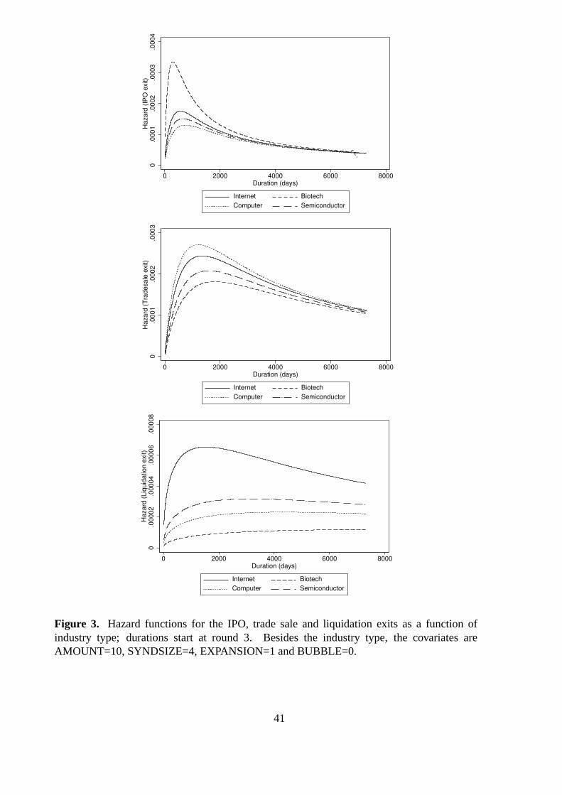
0.0

001

.0002

.0003

.0004

Hazard

(IP

O e

xit)

0 2000 4000 6000 8000Duration (days)

Internet Biotech

Computer Semiconductor

0.0

001

.0002

.0003

Hazard

(T

radesale

exit)

0 2000 4000 6000 8000Duration (days)

Internet Biotech

Computer Semiconductor

0.0

00

02

.00

00

4.0

00

06

.00

00

8H

aza

rd (

Liq

uid

atio

n e

xit)

0 2000 4000 6000 8000Duration (days)

Internet Biotech

Computer Semiconductor

Figure 3. Hazard functions for the IPO, trade sale and liquidation exits as a function ofindustry type; durations start at round 3. Besides the industry type, the covariates areAMOUNT=10, SYNDSIZE=4, EXPANSION=1 and BUBBLE=0.

41

0.0

001

.0002

.0003

.0004

Hazard

(IP

O e

xit)

0 2000 4000 6000 8000Duration (days)

Early Expansion

Later

0.0

001

.0002

.0003

.0004

.0005

Hazard

(IP

O e

xit)

0 2000 4000 6000 8000Duration (days)

Early Expansion

Later

0.0

00

1.0

00

2.0

00

3H

aza

rd (

IPO

exit)

0 2000 4000 6000 8000Duration (days)

Early Expansion

Later

Figure 4. Hazard functions (IPO exit) for the internet (top), biotech (middle) and computer(bottom) industries as a function of the type of stage; durations start at round 1. Besides theindustry and stage types, the covariates are AMOUNT=10, SYNDSIZE=4 and BUBBLE=0.

42

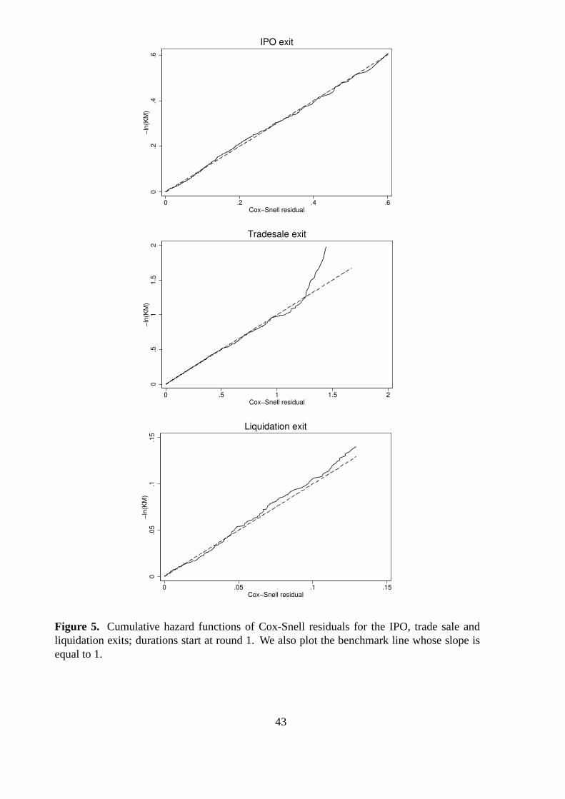
0.2

.4.6

−ln

(KM

)

0 .2 .4 .6Cox−Snell residual

IPO exit

0.5

11.5

2−

ln(K

M)

0 .5 1 1.5 2Cox−Snell residual

Tradesale exit

0.0

5.1

.15

−ln

(KM

)

0 .05 .1 .15Cox−Snell residual

Liquidation exit

Figure 5. Cumulative hazard functions of Cox-Snell residuals for the IPO, trade sale andliquidation exits; durations start at round 1. We also plot the benchmark line whose slope isequal to 1.

43

0.2

.4.6

−ln

(KM

)

0 .2 .4 .6Cox−Snell residual

IPO exit

0.5

11.5

2−

ln(K

M)

0 .5 1 1.5Cox−Snell residual

Tradesale exit

0.1

.2.3

.4−

ln(K

M)

0 .1 .2 .3Cox−Snell residual

Liquidation exit

Figure 6. Cumulative hazard functions of Cox-Snell residuals for the IPO, trade sale andliquidation exits; durations start at round 2. We also plot the benchmark line whose slope isequal to 1.

44

0.0

0005

.0001

.00015

Hazard

(IP

O e

xit)

0 2000 4000 6000 8000Duration (days)

West Northeast

South Midwest

0.0

0005

.0001

.00015

.0002

.00025

Hazard

(T

radesale

exit)

0 2000 4000 6000 8000Duration (days)

West Northeast

South Midwest

0.0

00

01

.00

00

2.0

00

03

.00

00

4.0

00

05

Ha

za

rd (

Liq

uid

atio

n e

xit)

0 2000 4000 6000 8000Duration (days)

West Northeast

South Midwest

Figure 7. Hazard functions for the IPO, trade sale and liquidation exits as a function of thegeographical location of the firm; durations start at round 1. Besides the geographical location,the covariates are COMPUTER=1, AMOUNT=10, SYNDSIZE=4 and EARLY=1.

45