A&A 593, A94 (2016)DOI: 10.1051/0004-6361/201628285c© ESO 2016

Astronomy&Astrophysics

Ionization fraction and the enhanced sulfur chemistry in Barnard 1A. Fuente1, J. Cernicharo2, E. Roueff3, 4, M. Gerin3, 4, J. Pety5, N. Marcelino6, R. Bachiller1, B. Lefloch7,

O. Roncero8, and A. Aguado9

1 Observatorio Astronómico Nacional (OAN,IGN), Apdo 112, 28803 Alcalá de Henares, Spaine-mail: a.fuente@oan.es

2 Instituto de Ciencia de Materiales de Madrid, ICMM-CSIC, C/ Sor Juana Inés de la Cruz 3, 28049 Cantoblanco, Spain3 CNRS UMR 8112, LERMA, Observatoire de Paris and École Normale Supérieure. 24 rue Lhomond, 75231 Paris Cedex 05, France4 Sorbonne Universités, UPMC Univ. Paris 06, UMR8112, LERMA, 75005 Paris, France5 Institut de Radioastronomie Millimétrique, 300 rue de la Piscine, 38406 Saint Martin d’Hères, France6 INAF, Osservatorio di Radioastronomia, via P. Gobetti 101, 40129 Bologna, Italy7 Institut de Planétologie et d’Astrophysique de Grenoble (IPAG) UMR 5274, Université UJF-Grenoble 1/CNRS-INSU,

38041 Grenoble, France8 Instituto de Física Fundamental (IFF-CSIC), C.S.I.C., Serrano 123, 28006 Madrid, Spain9 Facultad de Ciencias, Unidad Asociada de Química-Física Aplicada CSIC-UAM, Universidad Autónoma de Madrid,

28049 Madrid, Spain

Received 10 February 2016 / Accepted 7 May 2016

ABSTRACT

Context. Barnard B1b has been revealed as one of the most interesting globules from the chemical and dynamical point of view.It presents a rich molecular chemistry characterized by large abundances of deuterated and complex molecules. Furthermore, thisglobule hosts an extremely young Class 0 object and one candidate for the first hydrostatic core (FHSC) proving the youth of thisstar-forming region.Aims. Our aim is to determine the cosmic ray ionization rate, ζH2 , and the depletion factors in this extremely young star-formingregion. These parameters determine the dynamical evolution of the core.Methods. We carried out a spectral survey toward Barnard 1b as part of the IRAM large program “IRAM Chemical survey of sun-likestar-forming regions” (ASAI) using the IRAM 30-m telescope at Pico Veleta (Spain). This provided a very complete inventory ofneutral and ionic C-, N-, and S- bearing species with, from our knowledge, the first secure detections of the deuterated ions DCS+ andDOCO+. We use a state-of-the-art pseudo-time-dependent gas-phase chemical model that includes the ortho and para forms of H2,H+

2 , D+2 , H+

3 , H2D+, D2H+, D2, and D+3 to determine the local value of the cosmic ray ionization rate and the depletion factors.

Results. Our model assumes n(H2) = 105 cm−3 and Tk = 12 K, as derived from our previous works. The observational data arewell fitted with ζH2 between 3 × 10−17 s−1 and 10−16 s−1 and the elemental abundances O/H = 3 × 10−5, N/H = 6.4−8 × 10−5, C/H =1.7 × 10−5, and S/H between 6.0 × 10−7 and 1.0 × 10−6. The large number of neutral/protonated species detected allows us to derivethe elemental abundances and cosmic ray ionization rate simultaneously. Elemental depletions are estimated to be ∼10 for C and O,∼1 for N, and ∼25 for S.Conclusions. Barnard B1b presents similar depletions of C and O as those measured in prestellar cores. The depletion of sulfur ishigher than that of C and O, but not as extreme as in cold cores. In fact, it is similar to the values found in some bipolar outflows,hot cores, and photon-dominated regions. Several scenarios are discussed to account for these peculiar abundances. We proposethat it is the consequence of the initial conditions (important outflows and enhanced UV fields in the surroundings) and a rapidcollapse (∼0.1 Myr) that allows most S- and N-bearing species to remain in the gas phase to great optical depths. The interaction ofthe compact outflow associated with B1b-S with the surrounding material could enhance the abundances of S-bearing molecules, aswell.

Key words. astrochemistry – stars: formation – ISM: molecules – ISM: individual objects: Barnard 1 – ISM: abundances

1. Introduction

Cosmic rays (hereafter CRs) play a leading role in the chem-istry, heating, and dynamics of the interstellar medium (ISM).By ionizing their main component, molecular hydrogen, CRsinteract with dense molecular clouds, and this process initiatesa series of ion-molecule reactions that form compounds of in-creasing complexity to eventually build up the rich chemistryobserved in dark clouds (see, e.g., Wakelam et al. 2010). Also,CRs represent an important heating source for molecular clouds.Collisions with interstellar molecules and atoms convert abouthalf of the energy of primary and secondary electrons yielded

by the ionization process into heat (Glassgold & Langer 1973;Glassgold et al. 2012). Finally, the ionization fraction controlsthe coupling of magnetic fields with the gas, driving the dissipa-tion of turbulence and angular momentum transfer, thus playinga crucial role in protostellar collapse and the dynamics of accre-tion disks (see Padovani et al. 2013, and references therein).

The cosmic ray ionization rate ζH2 is the number of hydro-gen molecule ionization per second produced by CRs. In ab-sence of other ionization agents (X-rays, UV photons, J-typeshocks), the ionization fraction is proportional to

√ζH2 , which

becomes the key parameter in the molecular cloud evolution(McKee 1989; Caselli et al. 2002). During the last 50 yr, values

Article published by EDP Sciences A94, page 1 of 30

A&A 593, A94 (2016)

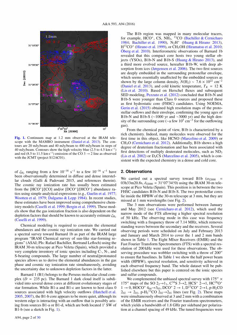
Fig. 1. Continuum map at 1.2 mm observed at the IRAM tele-scope with the MAMBO instrument (Daniel et al. 2013). The con-tours are 20 mJy/beam and 40 mJy/beam to 400 mJy/beam in steps of40 mJy/beam. Contours show the high velocity blue (2.5 to 4.5 km s−1)and red (8.5 to 11.5 km s−1) emission of the CO 3→ 2 line as observedwith the JCMT (project S12AC01).

of ζH2 ranging from a few 10−18 s−1 to a few 10−16 s−1 havebeen observationally determined in diffuse and dense interstel-lar clouds (Galli & Padovani 2015, and references therein).The cosmic ray ionization rate has usually been estimatedfrom the [HCO+]/[CO] and/or [DCO+]/[HCO+] abundance ra-tios using simple analytical expressions (e.g., Guelin et al. 1977;Wootten et al. 1979; Dalgarno & Lepp 1984). In recent studies,these estimates have been improved using comprehensive chem-istry models (Caselli et al. 1999; Bergin et al. 1999). These mod-els show that the gas ionization fraction is also dependent on thedepletion factors that should be known to accurately estimate ζH2

(Caselli et al. 1999).Chemical modeling is required to constrain the elemental

abundances and the cosmic ray ionization rate. We carried outa spectral survey toward Barnard 1b as part of the IRAM largeprogram “IRAM Chemical survey of sun-like star-forming re-gions” (ASAI; PIs: Rafael Bachiller, Bertrand Lefloch) using theIRAM 30-m telescope at Pico Veleta (Spain), which provided avery complete inventory of ionic species including C-, N-, andS-bearing compounds. The large number of neutral/protonatedspecies allows us to derive the elemental abundances in the gasphase and cosmic ray ionization rate simultaneously, avoidingthe uncertainty due to unknown depletion factors in the latter.

Barnard 1 (B1) belongs to the Perseus molecular cloud com-plex (D = 235 pc). The Barnard 1 dark cloud itself is subdi-vided into several dense cores at different evolutionary stages ofstar formation. While B1-a and B1-c are known to host class 0sources associated with high velocity outflows (Hatchell et al.2005, 2007), the B1-b core appears to be more quiet, although itswestern edge is interacting with an outflow that is possibly aris-ing from sources B1-a or B1-d, which are both located 1′ SW ofB1-b (see a sketch in Fig. 1).

The B1b region was mapped in many molecular tracers,for example, HCO+, CS, NH3, 13CO (Bachiller & Cernicharo1984; Bachiller et al. 1990), N2H+ (Huang & Hirano 2013),H13CO+ (Hirano et al. 1999), or CH3OH (Hiramatsu et al. 2010;Öberg et al. 2010). Interferometric observations of Barnard 1brevealed that this compact core hosts two young stellar ob-jects (YSOs), B1b-N and B1b-S (Huang & Hirano 2013), anda third more evolved source, hereafter B1b-W, with deep ab-sorption from ices (Jørgensen et al. 2006). The two first sourcesare deeply embedded in the surrounding protostellar envelope,which seems essentially unaffected by the embedded sources asshown by the large column density, N(H2) ∼ 7.6 × 1022 cm−2

(Daniel et al. 2013), and cold kinetic temperature, TK = 12 K(Lis et al. 2010). Based on Herschel fluxes and subsequentSED modeling, Pezzuto et al. (2012) concluded that B1b-N andB1b-S were younger than Class 0 sources and proposed theseas first hydrostatic core (FHSC) candidates. Using NOEMA,Gerin et al. (2015) obtained high resolution maps of the proto-stellar ouflows and their envelope, confirming the young ages ofB1b-N and B1b-S (∼1000 yr and ∼3000 yr) and the high den-sity of the surrounding core (∼a few 105 cm−3 for the outflowinggas).

From the chemical point of view, B1b is characterized by arich chemistry. Indeed, many molecules were observed for thefirst time in this object, like HCNO (Marcelino et al. 2009) orCH3O (Cernicharo et al. 2012). Additionally, B1b shows a highdegree of deuterium fractionation and has been associated withfirst detections of multiply deuterated molecules, such as ND3(Lis et al. 2002) or D2CS (Marcelino et al. 2005), which is con-sistent with the expected chemistry in a dense and cold core.

2. Observations

We carried out a spectral survey toward B1b (αJ2000 =03h33m20.8s, δJ2000 = 31◦07′34′′.0) using the IRAM 30-m tele-scope at Pico Veleta (Spain). This position is in between the twoFHSC candidates B1b-N and B1b-S. The two protostellar coreslie inside the HPBW of the 30-m telescope at 3 mm, but they aremissed at 1 mm wavelengths (see Fig. 2).

The 3 mm observations were performed between Januaryand May 2012 (see Cernicharo et al. 2012), which used thenarrow mode of the FTS allowing a higher spectral resolutionof 50 kHz. The observing mode in this case was frequencyswitching with a frequency throw of 7.14 MHz, which removesstanding waves between the secondary and the receivers. Severalobserving periods were scheduled on July and February 2013and January and March 2014 to cover the 1 and 2 mm bandsshown in Table 1. The Eight MIxer Receivers (EMIR) and theFast Fourier Transform Spectrometers (FTS) with a spectral res-olution of 200 kHz were used for these observations. The ob-serving procedure was wobbler switching with a throw of 200′′to ensure flat baselines. In Table 1 we show the half power beamwidth (HPBW), spectral resolution, and sensitivity achieved ineach observed frequency band. The whole dataset will be pub-lished elsewhere but this paper is centered on the ionic speciesand sulfur compounds.

We complemented the unbiased spectral survey with 175′′ ×175′′ maps of the SO 22→11, C34S 3→2, HCS+ 2→1, HC18O+

1→ 0, HOCO+ 404→303, DCO+ 2→ 1, D13CO+ 2→1, p-H2CO202 → 201, p-H2

13CO 202→201 lines (see Fig. 2). These mapswere simultaneously observed at 3 and 2 mm with a combinationof the EMIR receivers and the Fourier transform spectrometers,which yields a bandwidth of 1.8 GHz per sideband per polariza-tion at a channel spacing of 49 kHz. The tuned frequencies were

A94, page 2 of 30

A. Fuente et al.: Ionization fraction and the enhanced sulfur chemistry in Barnard 1

Fig. 2. Integrated intensity maps of the SO 22 → 11, C34S 3→2, HCS+ 2→1, HC18O+ 1→0, HOCO+ 404 → 303, DCO+ 2 → 1, D13CO+ 2 → 1,p-H2CO 202 → 201, and p-H13

2 CO 202 → 201 lines. The HPBW of the 30-m telescope at each line frequency is drawn in the bottom-left cornerof the panel. The stars indicate the positions of B1b-N, B1b-S and B1b-W. The black square shows the position targeted in the unbiased spectralsurvey.

Table 1. Observing and telescope parameters.

Freq (GHz) ∆v (km s−1) HPBWa Beff rms(Ta) (mK)82.5−117.6 0.1255 29′′−21′′ 0.81−0.78 3−5b

130.0−172.7 0.3424 19′′−14′′ 0.74 6−10c

200.6−275.9 0.2839 12′′−9′′ 0.63−0.49 5−10

Notes. (a) HPBW(arcsec) ≈ 2460/Freq(GHz); (b) rms ∼240 mK for ν >114 GHz; (c) rms∼500 mK for ν > 169 GHz.

85.55 and 144.90 GHz. We used the on-the-fly scanning strategywith a dump time of 0.5 s and a scanning speed of 10.9′′/s toensure a sampling of at least three dumps per beam at the 17.8′′resolution of the 2 mm lines. The 175′′ × 175′′ region was cov-ered using successive orthogonal scans along the RA and Decaxes. The separation between two successive rasters was 6.5′′(∼λ/2D) to ensure Nyquist sampling at the highest observed fre-quency, i.e., 145 GHz. A common reference position located atoffsets (200′′, 150′′) was observed for 10 seconds every 77.5 s.The typical IRAM 30 m position accuracy is 3′′.

The data reduction and line identification were carried outwith the package GILDAS1/CLASS software.

3. Methodology

Our goal is to use the database provided by the IRAM largeprogram ASAI together with previous millimeter data from ourgroup (Marcelino et al. 2005, 2009, 2010; Cernicharo et al.2012, 2013; Daniel et al. 2013; Cernicharo et al. 2014;Gerin et al. 2015) and complementary mapping to accuratelydetermine the fundamental chemical parameters.

Within our spectral survey we detected the following ions:HCO+, H13CO+, HC18O+, HC17O+, DCO+, D13CO+, HOCO+,DOCO+, HCS+, SO+, HC34S+, DCS+, HCNH+, H2COH+,HC3NH+, NNH+, NND+, N15NH+, and 15NNH+. This is prob-ably the first secure detection of the deuterated ions DCS+

and DOCO+. A tentative detection of DOCO+ was reported byFechtenbaum & Bontemps (2013) toward the massive protostarCIGX-N63. Daniel et al. (2013) modeled the emission of NNH+,NND+, N15NH+, and 15NNH+ ions in this core. We use their

1 See http://www.iram.fr/IRAMFR/GILDAS for more informationabout the GILDAS softwares (Pety 2005).

A94, page 3 of 30

A&A 593, A94 (2016)

results to compare with our chemical models without repeatingthe analysis. Our final list of detections is the most complete in-ventory of molecular ions observed in this source and, therefore,an unprecedented opportunity to improve our knowledge of theionization fraction. The main destruction mechanism of the ob-served protonated ions is the rapid recombination with e− to giveback the neutral parent species. For this reason, the [XH+]/[X]ratios are very sensitive to the gas ionization fraction and arecommonly used to estimate it. We also include the lines of theparent molecules in our analysis to compare with chemical mod-els (see Table A.1). It is interesting to note that we have not de-tected CO+ and HOC+. These ions react with molecular hydro-gen and only reach significant abundances in the external layersof photon-dominated regions that are not fully molecular (see,e.g., Fuente et al. 2003; Rizzo et al. 2003). The non-detection ofthese ions mainly supports the interpretation that we are probinga dense molecular core in which the ionization is dominated bycosmic rays.

The second key ingredient in gas-phase chemical mod-els is the depletion factors. The sensitivity of the chemistryto the elemental abundances in the gas phase was discussedby Graedel et al. (1982), who introduced the concept of “low-metal” elemental abundances, in which the abundances of met-als, silicon, and sulfur are depleted by a factor of 100 with re-spect to the values typically used until then (those observed inthe diffuse cloud ζ Oph). This choice of elemental abundancesprovides a reasonable agreement with the observed molecularabundances in dark clouds (see review by Agúndez & Wakelam2013). In recent decades, there has been increasing evidence thatthese abundances are decreasing with density because moleculesare frozen onto the grain surfaces and reach the lowest values indense prestellar cores. This phenomenon is quantified by the so-called depletion factor, that is, the ratio between the total (iceplus gas) abundance and that observed in the gas phase. The de-pletion is defined for a specific molecule or for the total amountof atoms of a given element. The depletion factor of each speciesdepends on the local physical conditions, time evolution, andbinding energy. For a given molecule, the depletion factor isevaluated by measuring the gas-phase abundance as a function ofthe gas density within the core. Tafalla et al. (2006) have shownthat CO presents a strong variation while the effect is moderatefor HCN and almost null for N2H+.

Determining the depletion factor of a given element is morecomplex, since it depends on the gas chemical composition and,eventually, on the binding energy of the compound(s) that arethe most abundant. To derive the elemental gas abundances ofC, O, N, and S, we need to include the main reservoirs of theseelements in our analysis. The CO abundance is four orders ofmagnitude larger than that of any other molecule except H2.Therefore, we can assume that in a dense core, such as B1b,all the carbon is locked in CO. The main reservoirs of nitrogenare atomic nitrogen (N) and molecular nitrogen (N2), which arenot observable. The nitrogen abundance can be derived by ap-plying a chemical model and fitting the observed abundances ofnitriles (HCN, HNC, and CN) and N2H+. The most abundantoxygenated molecules, O2, H2O, and OH, cannot be observedin the millimeter domain and the oxygen depletion factor hasto be derived indirectly. In the case of sulfur, the abundancesof S-bearing species are very sensitive to the C/O gas-phase ra-tio, and hence the oxygen depletion factor. A complete chemicalmodeling is needed to have a reasonable estimate of the O and Sdepletion factors.

4. Results

Figure B.1 shows the spectra of the neutral and protonatedspecies considered in this work. In all cases, the protonated andneutral species present similar line profiles suggesting that bothcome from the same region. All the lines show two narrow ve-locity components, at ∼6.5 km s−1 and ∼7.0 km s−1, respectively.We use the 30 m maps to explore the origin of the differentspecies and the two velocity components. The integrated inten-sity maps of the SO 22 → 11, C34S 3→ 2, HCS+ 2→1, HC18O+

1→0, HOCO+ 404→303, DCO+ 2→1, D13CO+ 2→1, p-H2CO202→201, and p-H2

13CO 202→201 lines are shown in Fig. 2. Theemission of the HC18O+, HOCO+, C34S, DCO+, D13CO+, andSO lines is concentrated in the elongated filament that containsB1b-N and B1b-S (see Fig. 2). The emission of the N2H+ 1→0line, as reported by Daniel et al. (2013), is also concentrated inthis dense filament. In the case of HOCO+, the elongated emis-sion seems to be slightly shifted to the west although the mapis too noisy to conclude. In all these cases, the line intensitiesare similar toward the N and S protostars. On the contrary, theemission of the o-NH2D 111s → 001a line peaks toward B1b-N(Daniel et al. 2013). Another exception is H2CO whose emis-sion presents an intense peak toward B1b-S. The emission of theHCS+ 2 → 1 line presents a flat spatial distribution suggestingthat this emission is coming from the cloud envelope.

Linewidths can also provide information about the originof the molecular emission. On basis of low angular resolutionobservations, Bachiller et al. (1990) proposed a correlation be-tween the linewidths and the depth into the B1 cloud with thenarrowest lines (∼1 km s−1) coming from the highest extinctionregions. Similar results were obtained by Daniel et al. (2013) onbasis of the observation of HCN, HNC, N2H+, NH3, and theirisotopologues. The line profiles were well reproduced by a col-lapsing dense core (infall velocity = 0.1 km s−1) with a turbu-lent velocity of 0.4 km s−1 surrounded by a static lower den-sity envelope with a turbulent velocity of 1.5 km s−1. In Fig. 3,we show the spatial distribution of the linewidths for the set ofmaps shown in Fig. 2. In agreement with previous works, wefind a clear decrease of the linewidth with the distance from thecore center in the SO 22 → 11 line. Linewidths are ∼2 km s−1

in the most external layer and decrease to ∼0.7 km s−1 towardthe core center. However, the linewidths of the HCS+ 2→1 linesare ∼2 km s−1 all over the region without a clear pattern. Thissupports the interpretation of the HCS+ emission coming froman external layer of the cloud. The only position where thelinewidths of the HCS+ line becomes <1 km s−1 is toward theIR star B1b-W. For HC18O+, DCO+, and D13CO+, we do seea trend, with the linewidths decreasing with the decreasing ra-dius from the core center. However, their linewidths are always>1 km s−1 suggesting that the emission is not dominated by theinnermost layers of the envelope. The linewidth of the p-H2COline is very constant over the whole core. This line is more likelyto be optically thick and its emission is only tracing the outerlayers of the core.

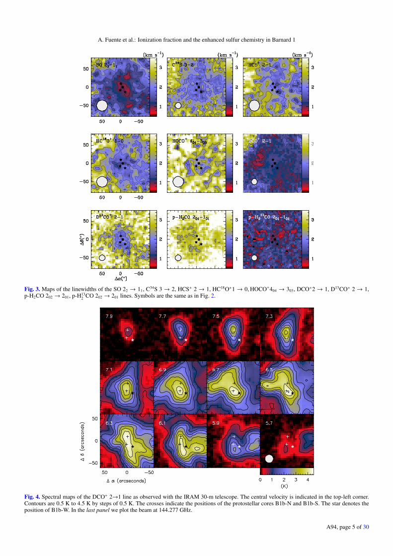
Figures 4 and 5 show the spectral maps of the DCO+ 2→1and SO 22→11 lines, respectively. The emission of DCO+ ex-tends from ∼5.5 km s−1 to ∼8.0 km s−1, while the SO emissionis detected in a narrower velocity range between ∼5.9 km s−1

to ∼7.5 km s−1, i.e., SO is mainly coming from the 6.5 km s−1

component. The intensity peak at 6.5 km s−1 is shifted ∼5′′west from the peak at 7.0 km s−1. It is interesting to note thatDCO+ presents an emission peak toward B1b-N at a veloc-ity of ∼7.5 km s−1 in agreement with the N2H+ and NH2Dobservations by Daniel et al. (2013). Recent interferometric

A94, page 4 of 30

A. Fuente et al.: Ionization fraction and the enhanced sulfur chemistry in Barnard 1

Fig. 3. Maps of the linewidths of the SO 22 → 11, C34S 3 → 2, HCS+ 2 → 1, HC18O+1 → 0,HOCO+404 → 303, DCO+2 → 1, D13CO+ 2 → 1,p-H2CO 202 → 201, p-H13

2 CO 202 → 201 lines. Symbols are the same as in Fig. 2.

Fig. 4. Spectral maps of the DCO+ 2→1 line as observed with the IRAM 30-m telescope. The central velocity is indicated in the top-left corner.Contours are 0.5 K to 4.5 K by steps of 0.5 K. The crosses indicate the positions of the protostellar cores B1b-N and B1b-S. The star denotes theposition of B1b-W. In the last panel we plot the beam at 144.277 GHz.

A94, page 5 of 30

A&A 593, A94 (2016)

Fig. 5. Spectral maps of the SO 22 → 11 line as observed with the IRAM 30-m telescope. The central velocity is indicated in the top-left corner.Contours are 0.5 K to 4.5 K by steps of 0.25 K. The crosses indicate the positions of the protostellar cores B1b-N and B1b-S. The star denotes theposition of B1b-W. In the last panel we plot the beam at 86.094 GHz.

observations revealed the kinematical structure of this regionat scales of ∼500–1000 AU (Huang & Hirano 2013; Gerin et al.2015). Huang & Hirano (2013) detected intense emission of theN2H+ and N2D+ 3 → 2 lines toward the two protostellar coresB1b-N and B1b-S using the SMA. The N2D+ emission is cen-tered at ∼7.0±0.2 km s−1 toward B1b-N and at ∼6.5±0.2 km s−1

toward B1b-S, confirming the existence of the two velocitycomponents.

In the cases of H213CO, H2S, HOCO+, and in one transition

of CCS, OCS, and SO2 (see Table B.1), we detect wings at red-shifted velocities. Compact outflows are detected toward eachprotostellar core with wings in the 0 to 15 km s−1 velocity range(Gerin et al. 2015). In Fig. 6 we overlay the 30 m beam at 3 mmand 1 mm on the interferometric H2CO map. The B1b-N out-flow and the red wing of the B1b-S outflow lie within our beamat 3 mm, but the whole B1b-N outflow and a fraction of the redlobe of the B1b-S outflow are missed in the 2 mm and 1 mmobservations. The emission at the outflow velocities is not takeninto account in our calculations because we are only interested inthe two velocity components associated with the core emission(see Sect. 5 for details).

5. Column density calculationsIn order to investigate abundance variations between the two ve-locity components, we carried out a separate analysis for each.The spectral resolution of our observations is different for the3 mm, 2 mm and 1 mm bands. To carry out a uniform analy-sis, we degraded the velocity resolution to a common value of0.25 km s−1 and then fitted Gaussians to each one. In the fitting,we fixed the central velocities to 6.5 km s−1 and ∼7.0 km s−1, andthe linewidths to ∆v = 0.7 km s−1 and 1.0 km s−1, respectively.The fitting returns the integrated intensity for each component.This procedure gives an excellent fit for most lines and neglects

Fig. 6. Interferometric integrated intensity map of the outflows asso-ciated with B1b-N and B1b-S in the H2CO 20,2–10,1 line (Gerin et al.2015). The crosses indicate the positions of the protostellar cores,B1b-N and B1b-S, and the star, of B1b-W. The position targeted byour spectral survey is drawn with a white square and the beams of the30-m telescope at 3 mm and 1 mm are indicated by white circles.

possible line wings with velocities >7.5 km s−1. The final inte-grated intensities are shown in Table B.1. We are aware that thissimple method is not able to cleanly separate the contributionfrom each component. There is some unavoidable velocity over-lap between the two components along the line of sight and ourspatial resolution is limited (see Figs. 4 and 5). In spite of that,our simple method help to detect possible chemical gradients.

Several isotopologues of each molecule were detected asexpected taking the large extinction in this core into account

A94, page 6 of 30

A. Fuente et al.: Ionization fraction and the enhanced sulfur chemistry in Barnard 1

Table 2. Column density calculations.

Molecule LTE LVG1

6.5 km s−1 7.0 km s−1 Total 6.5 km s−1 7.0 km s−1 TotalTrot(K) NX(cm−2) Trot(K) NX(cm−2) NX(cm−2) NX(cm−2) NX(cm−2) NX(cm−2)

Ions IonsHC18O+ 4.4+0.2

−0.2 1.7+0.1−0.1 × 1011 4.2+0.4

−0.7 1.5+0.2−0.3 × 1011 3.2 × 1011 2.0+0.1

−0.1 × 1011 1.4+0.2−0.3 × 1011 3.4 × 1011

D13CO+ 7.8+0.5−0.5 1.2+0.2

−0.2 × 1011 4.5+0.2−0.2 3.9+0.5

−0.5 × 1011 5.1 × 1011 2.0+0.1−0.1 × 1011 4.5+0.1

−0.1 × 1011 6.5 × 1011

HOCO+ 11.9+0.3−0.3 5.2+0.3

−0.3 × 1011 10.7+1.3−1.0 2.4+1.0

−0.7 × 1011 7.6 × 1011 5.2+0.2−0.2 × 1011 3.0+0.2

−0.2 × 1011 8.2 × 1011

DOCO+ 11a 7.0+0.9−0.9 × 1010 11a 4.0+2.0

−2.0 × 1010 1.1 × 1011 9.0+1.1−1.1 × 1010 5.0+2.0

−2.0 × 1010 1.1 × 1011

SO+ 9.0+0.8−0.7 7.6+2.0

−1.6 × 1011 8.3+2.2−1.4 4.8+4.1

−2.2 × 1011 1.2 × 1012

HCS+ 10.6+6.5−3.0 2.1+3.6

−1.3 × 1011 7.5+0.5−0.6 6.2+0.2

−0.2 × 1011 8.3 × 1011 5.5+0.1−0.1 × 1011 5.5+0.1

−0.1 × 1011 1.1 × 1012

DCS+ 10b 5.0+1.0−1.0 × 1010 5.0 × 1010 4.5+1.1

−1.1 × 1010 4.5 × 1010

HCNH+ 29.0+50−12 5.1+4.1

−0.7 × 1012 8.9+5.3−2.9 3.8+1.5

−0.5 × 1012 8.9 × 1012 3.7+0.4−0.4 × 1012 4.0+0.4

−0.4 × 1012 7.7 × 1012

H2COH+ 10b 2.0+1.0−1.0 × 1011 2.0+1.0

−1.0 × 1011

CO+ 10b <6.0 × 1010 <6.0 × 1010

HOC+ 10b <2.0 × 1010 <2.0 × 1010

Neutrals Neutrals13C18O 5.5+1.3

−0.9 2.4+0.2−0.2 × 1013 10.9+0.9

−1.4 5.2+0.1−0.1 × 1013 7.6 × 1013 3.0+0.2

−0.2 × 1013 6.0+0.3−0.3 × 1013 9.0 × 1013

o-H213CO 5.5+0.8

−0.6 6.1+2.1−1.5 × 1011 5.2+0.9

−0.3 4.9+3.2−1.9 × 1011 1.1 × 1012 1.1+0.6

−0.6 × 1012 1.3+0.7−0.7 × 1012 2.4 × 1012

13CS 7.1+1.6−1.1 7.8+2.0

−5.7 × 1011 3.2+0.4−0.7 3.1+3.2

−1.6 × 1012 3.9 × 1012 1.3+0.1−0.1 × 1012 9.0+0.3

−0.3 × 1011 2.2 × 1012

S18O 6.8+0.6−0.6 1.6+0.6

−0.5 × 1012 8.2+2.0−1.4 0.6+0.4

−0.3 × 1012 2.3 × 1012 2.2+0.1−0.1 × 1012 8.0+0.3

−0.3 × 1011 3.0 × 1012

33SO 12.3+7.3−4.0 1.6+1.0

−0.6 × 1012 18.9+71−8.3 0.7+0.7

−0.4 × 1012 2.3 × 1012 3.8+0.1−0.1 × 1012 6.0+2.0

−2.0 × 1011 4.4 × 1012

34SO2 5.8+2.0−1.2 1.1+1.0

−0.5 × 1012 1.1+0.1−0.1 × 1012

SO2 10.1+1.0−1.0 7.9+3.0

−2.0 × 1012 10.2+2.0−1.2 2.9+1.3

−0.9 × 1012 1.1 × 1013 1.6+0.1−0.1 × 1013 4.5+0.1

−0.1 × 1012 2.0 × 1013

OC34S 8.7+0.6−0.5 1.2+0.2

−0.2 × 1012 1.0+0.3−0.3 × 1012

OCS 11.7+13.0−4.0 1.5+0.9

−0.6 × 1013 20.4+1.4−1.3 4.9+0.6

−0.6 × 1012 1.9 × 1013 1.7+0.1−0.1 × 1013 8.0+4.0

−4.0 × 1011 1.7 × 1013

H213CSc 7.4 1.6+0.3

−0.3 × 1011

CCS 8.3+0.7−0.6 5.9+2.4

−1.7 × 1012 8.2+0.7−0.6 3.6+1.3

−1.0 × 1012 9.5 × 1012 9.3+0.1−0.1 × 1012 5.2+0.1

−0.1 × 1012 1.4 × 1013

CC34S 3.5+0.7−0.7 × 1011 2.5+0.7

−0.7 × 1011 6.0 × 1011

CCCS 8.6+1.6−1.2 2.2×1012

o-H2S 10d 7.0+0.2−0.2 × 1012 10 3.0+0.2

−0.2 × 1012 1.0 × 1013

NS 10d 5.4+0.2−0.2 × 1012 10 9.0+0.2

−0.2 × 1012 1.4 × 1013

Notes. (1) LVG calculations assuming Tk = 12 K and n(H2) = 105 cm−3; (a) assuming the rotation temperature of HOCO+; (b) assuming therotation temperature of HCS+; (c) in this case the ortho and para species are treated together (ortho-to-para(OTP) = 3) and we assumed the rotationtemperature calculated for H2CS by Marcelino et al. (2005); (d) reasonable guess for the rotation temperature.

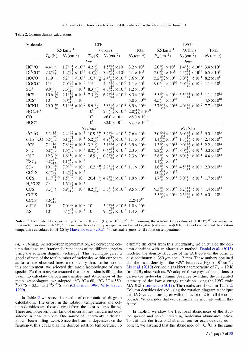
(Av ∼ 76 mag). As zero-order approximation, we derived the col-umn densities and fractional abundances of the different speciesusing the rotation diagram technique. This technique gives agood estimate of the total number of molecules within our beamas far as the observed lines are optically thin. To be sure ofthis requirement, we selected the rarest isotopologue of eachspecies. Furthermore, we assumed that the emission is filling thebeam. To calculate the column densities and abundances of themain isotopologues, we adopted 12C/13C = 60, 16O/18O = 550,32S/34S = 22.5, and 34S/33S = 6 (Chin et al. 1996; Wilson et al.1999).

In Table 2 we show the results of our rotational diagramcalculations. The errors in the rotation temperatures and col-umn densities are those derived from the least squares fitting.There are, however, other kind of uncertainties that are not con-sidered in these numbers. One source of uncertainty is the un-known beam filling factor. Since the beam is dependent on thefrequency, this could bias the derived rotation temperature. To

estimate the error from this uncertainty, we calculated the col-umn densities with an alternative method. Daniel et al. (2013)modeled the density structure of the B1b core on the basis ofdust continuum at 350 µm and 1.2 mm. These authors obtainedthat the mean density in the ∼29′′ beam is n(H2) ≈ 105 cm−3.Lis et al. (2010) derived a gas kinetic temperature of TK = 12 Kfrom NH3 observations. We adopted these physical conditions toderive the molecular column densities by fitting the integratedintensity of the lowest energy transition using the LVG codeMADEX (Cernicharo 2012). The results are shown in Table 2.Column densities derived using the rotation diagram techniqueand LVG calculations agree within a factor of 2 for all the com-pounds. We consider that our estimates are accurate within thisfactor.

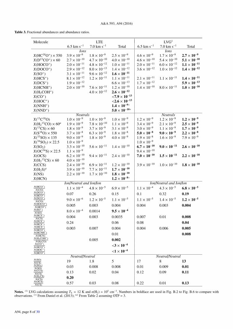
In Table 3 we show the fractional abundances of the stud-ied species and some interesting molecular abundance ratios.To estimate the fractional abundances for each velocity com-ponent, we assumed that the abundance of 13C18O is the same

A94, page 7 of 30

A&A 593, A94 (2016)

Table 3. Fractional abundances and abundance ratios.

Molecule LTE LVG1

6.5 km s−1 7.0 km s−1 Total 6.5 km s−1 7.0 km s−1 TotalIons Ions

X(HC18O+) × 550 3.9 × 10−9 1.8 × 10−9 2.5 × 10−9 4.6 × 10−9 1.7 × 10−9 2.7 × 10−9

X(D13CO+) × 60 2.7 × 10−10 4.7 × 10−10 4.0 × 10−10 4.6 × 10−10 5.4 × 10−10 5.1 × 10−10

X(HOCO+) 2.0 × 10−11 4.8 × 10−12 1.0 × 10−11 2.0 × 10−11 6.0 × 10−12 1.1 × 10−11

X(DOCO+) 2.9 × 10−12 8.0 × 10−13 1.4 × 10−12 3.6 × 10−12 1.0 × 10−12 1.4 × 10−12

X(SO+) 3.1 × 10−11 9.6 × 10−12 1.6 × 10−11

X(HCS+) 8.1 × 10−12 1.2 × 10−11 1.1 × 10−11 2.1 × 10−11 1.1 × 10−11 1.4 × 10−11

X(DCS+) 1.9 × 10−12 6.6 × 10−13 1.7 × 10−12 5.9 × 10−13

X(HCNH+) 2.0 × 10−10 7.6 × 10−11 1.2 × 10−10 1.4 × 10−10 8.0 × 10−11 1.0 × 10−10

X(H2COH+) 4.0 × 10−12 2.6 × 10−12

X(CO+) <7.9 × 10−13

X(HOC+) <2.6 × 10−13

X(NNH+) 1.4 × 10−9∗

X(NND+) 5.0 × 10−10∗

Neutrals NeutralsX(13C18O) 1.0 × 10−9 1.0 × 10−9 1.0 × 10−9 1.2 × 10−9 1.2 × 10−9 1.2 × 10−9

X(H213CO) × 60a 1.9 × 10−9 7.8 × 10−10 1.1 × 10−9 3.4 × 10−9 2.1 × 10−9 2.5 × 10−9

X(13CS) × 60 1.8 × 10−9 3.7 × 10−9 3.1 × 10−9 3.0 × 10−9 1.1 × 10−9 1.7 × 10−9

X(S18O) × 550 3.7 × 10−8 6.3 × 10−9 1.8 × 10−8 5.0 × 10−8 9.0 × 10−9 2.2 × 10−8

X(33SO) × 135 9.0 × 10−9 1.8 × 10−9 4.0 × 10−9 1.9 × 10−8 1.6 × 10−9 7.9 × 10−9

X(34SO2) × 22.5 1.0 × 10−9 1.0 × 10−9

X(SO2) 3.3 × 10−10 5.6 × 10−11 1.4 × 10−10 6.7 × 10−10 9.0 × 10−11 2.6 × 10−10

X(OC34S) × 22.5 1.1 × 10−9 9.4 × 10−10

X(OCS) 6.2 × 10−10 9.4 × 10−11 2.4 × 10−10 7.0 × 10−10 1.5 × 10−11 2.2 × 10−10

X(H213CS) × 60 4.0 × 10−10

X(CCS) 2.4 × 10−10 6.9 × 10−11 1.2 × 10−10 3.9 × 10−10 1.0 × 10−10 1.8 × 10−10

X(H2S)a 3.9 × 10−10 7.7 × 10−11 1.7 × 10−10

X(NS) 2.2 × 10−10 1.7 × 10−10 1.8 × 10−10

X(HCN) 1.2 × 10−8∗

Ion/Neutral and Ion/Ion Ion/Neutral and Ion/IonN(HCO+)

N(CO) 1.1 × 10−4 4.8 × 10−5 6.9 × 10−5 1.1 × 10−4 4.3 × 10−5 6.8 × 10−5

N(DCO+)N(HCO+) 0.07 0.26 0.15 0.1 0.32 0.19N(DCO+)

N(CO) 9.0 × 10−6 1.2 × 10−5 1.1 × 10−5 1.1 × 10−5 1.4 × 10−5 1.2 × 10−5

N(HOCO+)N(HCO+) 0.005 0.003 0.004 0.004 0.003 0.004

N(SO+)N(SO) 8.0 × 10−4 0.0014 9.5 × 10−4

N(HCS+)N(CS) 0.004 0.003 0.0035 0.007 0.01 0.008

N(DCS+)N(HCS+) 0.24 0.06 0.08 0.04N(HCS+)N(HCO+) 0.003 0.007 0.004 0.004 0.006 0.005N(HCNH+)

N(HCN) 0.01 0.008N(H2COH+)

N(H2CO) 0.005 0.002N(CO+)

N(HCO+) <3 × 10−4

N(HOC+)N(HCO+) <1 × 10−4

Neutral/Neutral Neutral/NeutralN(SO)N(CS) 19 1.8 5 17 8 13N(SO2)N(SO) 0.03 0.008 0.008 0.01 0.009 0.01N(CCS)N(CS) 0.13 0.02 0.04 0.12 0.09 0.11

N(H2CS)N(CS) 0.20

N(OCS)N(CS) 0.57 0.03 0.08 0.22 0.01 0.13

Notes. (1) LVG calculations assuming Tk = 12 K and n(H2) = 105 cm−3. Numbers in boldface are used in Fig. B.2 to Fig. B.6 to compare withobservations. (∗) From Daniel et al. (2013); (a) From Table 2 assuming OTP = 3.

A94, page 8 of 30

A. Fuente et al.: Ionization fraction and the enhanced sulfur chemistry in Barnard 1

for the two components and adopted a total molecular hydrogencolumn density of N(H2) = 7.6 × 1022 cm−2 (Daniel et al.2013). Most of the fractional abundances and abundance ra-tios agree within the uncertainties for the two velocity compo-nents. There are, however, significant chemical differences forsome species. One difference is that the HCO+ deuterium frac-tion is a factor ∼3 higher in the 7 km s−1 component than in the6.5 km s−1 one. The spectral velocity maps of the DCO+ 2→1and D13CO+ 2→1 lines show that the 7 km s−1 component isassociated with the cold protostar B1b-N. The second differenceis that the SO/CS abundance ratio is 2−10 times larger in the∼6.5 km s−1 component than in the ∼7.0 km s−1 component.High SO abundances, up to ∼10−7, are found in bipolar out-flows because of the release of sulfuretted compounds into thegas phase (Bachiller & Pérez Gutiérrez 1997). One could thinkthat the high SO abundances could then result from the interac-tion of the cold core with the B1b-S outflow, or, more likely, ofthe interaction of the dense core with the B1a and/or B1d out-flows. However, the profiles of the SO lines are very narrow,which is contrary to one would expect if the emission were com-ing from a shock or a turbulent medium. In Sect. 6, we discussin detail the sulfur chemistry and possible explanations for thehigh SO abundance in Barnard 1.

One important result is that the [XH+]/[X] ratios do notpresent variations between the two velocity components. Thissupports our interpretation that the ionization fraction is mainlydriven by CR and is consistent with the measured H2 columndensity (7.6× 1022 cm−2). The core is expected to be thoroughlypermeable to CR and the ionization does not present significantfluctuations across the envelope.

6. Chemical modeling

We perform chemical modeling to constrain the physical andchemical properties in B1b. We do not include here the ac-cretion/desorption mechanisms of gas-phase molecules on thegrains and instead vary the amount of elemental abundances ofheavy atoms available in the gas phase to mimic these effects.We explicitly consider, however, the formation on grains of themolecular hydrogen, H2, and the isotopic substituted forms HDand D2. Such an approach, although primitive, allows us to dis-entangle the main gas-phase processes at work. We use both asteady-state and time-dependent model to explore the chemistryand verified that the steady-state results are recovered by thetime-dependent code for sufficiently large evolution time (typ-ically 10 Myr).

Our chemical network contains 261 species linked throughmore than 5636 chemical reactions. Ortho and para forms of H2,H+

2 , H+3 , D2, H2D+, D2H+, and D+

3 are explicitly introduced, fol-lowing the pioneering papers of Flower et al. (2004, 2006) forheavily depleted regions, and including the chemistry of car-bon, oxygen, nitrogen, and sulfur. Discriminating between paraand ortho forms of H2 is particularly critical for deuteration incold regions via the H+

3 + HD ↔ H2D+ + H2 reaction as theendothermicity of the reverse reaction is of the same order ofmagnitude as the rotational energy of H2, as first emphasized byPagani et al. (1992). Nitrogen chemistry is also very sensitive tothe ortho and para forms of H2, as pointed out by Le Bourlot(1991), because of the small endoergicity of the N+ + H2 →

NH+ + H reaction. Whereas a definitive understanding of thisreaction is still pending (Zymak et al. 2013), we follow the pre-scription of Dislaire et al. (2012) for the reaction rate coeffi-cients of N+ + H2(p/o) reaction. Our chemical network alsocontains the recent updates coming from experimental studies

of reactions involving neutral nitrogen atoms as reviewed inWakelam et al. (2013). We also introduced species containingtwo nitrogen atoms, such as C2N2 and C2N2H+, following therecent detection of C2N2H+ by Agúndez et al. (2015) for whichthe reaction rate coefficients have essentially been taken fromthe UMIST astrochemical database (McElroy et al. 2013). Animportant feature that is not fully recognized is the link betweensulfur and nitrogen chemistry as shown by the detection of NS,which is found both in regions of massive star formation and incold dark clouds (McGonagle et al. 1994; McGonagle & Irvine1997). The main formation reaction is through S + NH whoserate is given as 10−10 cm3 s−1 in astrochemical databases, whichthen also induces that sulfur chemistry may depend on o/p ratioof H2.

Our methodology is the following: We run the time-dependent model for a set of standard elemental abundances andcosmic ray ionization rates to determine which molecular abun-dances and molecular abundance ratios reach the steady state ina few 0.1−1 Myr, which is the estimated age for B1b. Thesemolecular abundances and abundance ratios are expected to bein equilibrium and are used to explore the parameter space us-ing steady-state calculations. On basis of the steady-state calcu-lations, we select the most plausible values and run the time-dependent model to confirm that our fit is correct. In all ourcalculations, we assume uniform physical conditions and fixn(H2) = 105 cm−3 and Tk = 12 K, according with previousworks (Lis et al. 2010; Daniel et al. 2013). We iterate severaltimes to get the best match with the observations. The predic-tions of our best-fit model are compared with observations inFigs. B.2 and B.3.

6.1. Cosmic ray ionization rate

The [HCO+]/[CO] ratio has been extensively used to estimatethe cosmic ray ionization rate. The results of our time dependentmodel confirms that it is, very likely, the most reliable diagnosticsince it reaches the equilibrium in 0.1 Myr and its chemistry iswell known. Other [XH+]/[X] ratios, such as [HCS+]/[CS] and[HCNH+]/[HCN], are also expected to be in equilibrium at thetypical ages of a molecular cloud. Figure B.4 shows the varia-tion of the [HCO+]/[CO], [HCNH+]/[HCN], and [HCS+]/[CS]as a function of the cosmic ray ionization rate in steady-statecalculations. Assuming an uncertainty of a factor of 2 in thederived abundance ratios, values of ζH2 in the interval between3 × 10−17 s−1 to 1 × 10−16 s−1 are consistent with the observed[HCO+]/[CO] and [HCNH+]/[HCN] ratios. These values are atthe upper end of the values inferred for cloud cores (Caselli et al.1998) and are higher than those of the typical dark cloud L1544,ζH2 ∼ 1× 10−18 (Galli & Padovani 2015). This could explain thehigher gas and dust temperature in this dense core of Td ∼ 12 K,compared with dust temperature in L1544 of Td < 6–8 K(Crapsi et al. 2007).

The [HCS+]/[CS] ratio is not fitted by any reasonable valueof ζH2 . This is not surprising since the HCS+ emission is mainlycoming from the low density envelope. In Fig. B.2 we showmodel predictions for a density of n(H2) = 104 cm−3. The abun-dances of most molecules decrease while the HCS+ abundanceremains constant and that of CCS increases. These calculationswere carried out assuming the same elemental abundances asin the high density case. This is not realistic since lower de-pletions are expected in the envelope and, therefore, the HCS+

abundance would be higher. Moreover, this core is illuminatedon its eastern side by the nearby Herbig Ae stars LkHα 327and LkHα 328 (Walawender et al. 2009; Young et al. 2015). The

A94, page 9 of 30

A&A 593, A94 (2016)

UV photons are expected to increase the HCS+ abundance. Infact, the HCS+2 → 1 emission is maximum toward the illumi-nated side (see Fig. 2).

Our estimate of the cosmic ray ionization rate permits us toobtain an estimate of the N2 abundance in this core. Since it isone of the main nitrogen reservoirs, N2 cannot be observed at(sub)millimeter wavelengths because of its lack of dipole mo-ment. We can only estimate its abundance indirectly through theprotonated compound, N2H+. The N2H+ abundance is very sen-sitive to the cosmic ray ionization rate. In Fig. B.4, we presentthe [N2H+]/[N2] ratio as a function of the cosmic ray ionizationrate. Assuming ζH2 = 4 × 10−17 s−1 and on the basis of our ob-servational data, we derive [N2] ∼ 8 × 10−5, which is consistentwith the typical value of the N elemental abundance in a darkcloud, N/H = 6.4 × 10−5.

The HOCO+ molecule (protonated carbon dioxide) isthought to form via a standard ion-molecule reaction, the trans-fer of a proton from H+

3 to CO2 (see, e.g., Turner et al. 1999).To date HOCO+ has been detected toward the Galactic center,a few starless translucent clouds (Turner et al. 1999), a singlelow-mass Class 0 protostar (Sakai et al. 2008), and the proto-stellar shock L1157-B1 (Podio et al. 2014). Interestingly, thismolecule is particularly abundant, ∼10−9, in the Galactic centerregion (Minh et al. 1988, 1991; Deguchi et al. 2006; Neill et al.2014). We derive an HOCO+ abundance of ∼10−11, i.e, two or-ders of magnitude lower than that derived in the Galactic cen-ter clouds (Deguchi et al. 2006; Neill et al. 2014) and L1157-B1(Podio et al. 2014), and a factor of ∼10 lower than that in translu-cent clouds (Turner et al. 1999). This is not unexpected since theHOCO+ abundance is inversely proportional to the gas density(Sakai et al. 2008) and B1b is a dense core. Our model under-predicts the HOCO+ abundance by a factor 200 (see Fig. B.2).As commented below, HOCO+ is proxy of CO2, which is notefficiently formed in the gas phase (Turner et al. 1999).

The lack of an electric dipole moment of CO2 makes gas-phase detections difficult. The abundance of CO2 in the solidphase has been investigated through its two vibrational modesat 4.3 and 15.0 µm. In the solid phase, the typical abundanceis ∼10−6 relative to total H2 (Gerakines et al. 1999; Gibb et al.2004). In the gas phase, the typical detected abundance is1–3 × 10−7 (van Dishoeck et al. 1996; Boonman et al. 2003;Sonnentrucker et al. 2006). Assuming the [HOCO+]/[CO2] ratiopredicted by our model, 2.2 × 10−4, we estimate a CO2 abun-dance of ∼5 × 10−8. This value is at the lower end of those mea-sured in star-forming regions but 200 times larger than that pre-dicted by our gas-phase model. Photodesorption and sputteringof the icy mantles are more likely to be the main CO2 productionmechanisms.

6.2. Sulfur chemistry: C, O, and S elemental abundances

The initial elemental abundances in the gas phase are an essen-tial parameter in the chemical modeling. In cloud cores (Av >10 mag), as long as the C elemental abundance is lower thanO, we can assume that the abundance of C is equal to that ofCO and conclude that C/H = 1.7 × 10−5; we note that fractionalabundances are given with respect to H2. The main source ofuncertainty in this value comes from the uncertainty in the COabundance, which is estimated to be a factor of 2.

To estimate the amount of S in the gas phase requires a de-tailed modeling of its chemistry. As shown in Fig. B.5, the cos-mic ray ionization rate is a critical paramenter to estimate theS/H. The main sulfur reservoirs in a dense core are atomic sulfur(S) and SO (see Fig. 7). Unfortunately, chemical models make a

Fig. 7. Predicted fractional abundances using the same parameters asin Fig. B.2. The abundances of SO, SO2 and SO+, and O2 dramaticallyincrease after 1 Myr.

poor work in predicting the fractional abundance of SO, becausethe predicted SO abundance depends on two uncertain factors: i)the S + O2 → SO + O and S + OH→ SO + H reaction rates andii) the O2 and OH abundances.

The S + O2 reaction rate coefficient at low temperatures isnot known. Experimental measurements have only been per-formed above 200 K. Lu et al. (2004) reviewed the varioustheoretical and experimental results and adopted a value of2 × 10−12 cm3 s−1 at 298 K. The UMIST and KIDA databasessuggest different values. In KIDA, a constant value of 2.1 ×10−12 cm3 s−1 is suggested in the 250−430 K temperature rangewhereas the latest version of the UMIST database gives 1.76 ×10−12 (T /300)0.81 exp(30.8/T ) cm3 s−1 in the 200−3460 K tem-perature interval. This small activation barrier would imply ratesas low as 10−23 cm3 s−1 at the temperature of 12 K and a de-crease in the SO, SO2, and SO+ abundances. Quasiclassical tra-jectory calculations were carried out for the reaction S + O2 andits reverse by Rodrigues & Varandas (2003). With 6000 trajec-tories they obtain that the reaction rate remains constant or de-creases very slowly for temperatures between 50 K and 1000 K.Using the same potential, we performed new quasiclassical tra-jectory calculations with 100 000 trajectories for temperaturesbetween 10 K and 50 K (see Appendix A). Our results confirmthat the reaction rate remains very constant (within 30%) in the10 K to 50 K range. Therefore, we adopted the KIDA value,2.1 × 10−12 cm3 s−1, in our calculations.

The second more important reaction for the formation ofSO is S + OH. DeMore et al. (1997) measured a value of6.6 × 10−11 cm3 s−1 at 398 K, which is the value adopted in ourcalculations. Recent theoretical calculations by Goswami et al.(2014) predicted a value a factor of ∼2 lower. These calculationswere performed for a range of temperatures between 10−500 Kand the reaction rate remains very constant over this range withan increase of a factor of ∼1.6 for temperatures close to 10 K.

A94, page 10 of 30

A. Fuente et al.: Ionization fraction and the enhanced sulfur chemistry in Barnard 1

Our adopted experimental value is very likely good by a factorof 2 for the physical conditions of B1.

The oxygen and sulfur chemistries are tightly linked. SinceS is rapidly converted to SO by reacting with O2 and OH, itsabundance is very dependent on the amount of molecular oxy-gen in the gas phase, that itself depends on the C/O ratio (seeFig. B.6). Conversely, a large abundance of S in the gas phase(>10−6) leads to a rapid destruction of O2 and decreases the[O2]/[O] ratio (see Fig. B.5). We find a good agreement withthe observations, assuming C/O = 0.6 and S/H in the intervalbetween 6 × 10−7 and 10−6. With these parameters we have anexcellent fit of the SO abundance and the [SO]/[CS], [SO2/[SO],and [H2CS]/[CS] ratios, although the agreement is worse forOCS (Figs. B.5 and B.6). We do not have a good explanationfor the low observed abundance of OCS. It may be frozen ontothe grain mantles in this cold core. Taking into account the lim-itations of our model, of one single n(H2) and T , we consider,however, that the overall agreement with observational data isquite good. Assuming these values, our chemical model predictsa steady-state O2 abundance of ∼4 × 10−7. There is no measure-ment of the O2 abundance in B1b, but this predicted abundanceis higher than the upper limits derived for other dark clouds(Pagani et al. 2003) and that reported in ρ Oph A (∼5 × 10−8)(Liseau et al. 2012). The low O2 abundance measured in darkclouds is usually explained in terms of time evolution. O2 is alate-type molecule that presents low abundance (∼10−8) at typ-ical ages of dark clouds (a few 0.1 Myr). Another possibility isthat O2 becomes frozen on grain mantles. Regarding the sulfurchemistry, a lower O2 abundance would decrease the SO pro-duction via the S + O2 reaction. In this case, we would needto increase S/H to reproduce the observations and our estimatewould be a lower limit.

Finally, our chemical model does not include surface chem-istry. The main effect of dust grains is to decrease the abundanceof sulfur bearing molecules, especially SO2, because of adsorp-tion on grain mantles. The most abundant species in Barnard 1b,SO, is thought to form in the gas phase. As long as this remainstrue, we consider that our measurement of the sulfur depletion isreliable.

7. Barnard 1b chemistry

We have used a state-of-the-art, gas-phase model to derive thecosmic ionization rate and elemental abundances toward thedense core Barnard 1b. Our model fit predicts the observed abun-dances and abundance ratios reasonably well (within a factor oftwo), but it fails, by several orders of magnitude to predict theabundances of HCS+ and HOCO+. As commented above, HCS+

is very likely coming from the lower density envelope instead ofthe dense core and cannot be accounted by our single point (n,T )model. In the case of HOCO+, the model failure is not surprisingsince CO2 is mainly formed by surface reactions.

In Table 4 we compare the initial abundances derived to-ward B1b with typical values in dark clouds and diffuse clouds(Agúndez & Wakelam 2013). The depletion of C and O is tentimes larger than those measured in prototypical dark cloudssuch as TMC 1 and L134N. These values are similar to thosefound in prestellar cores and young stellar objects where highvalues of CO depletion (∼5−10) and high deuterium fractions(∼0.01) are measured (Caselli et al. 1999; Jørgensen et al. 2002;Crapsi et al. 2005; Emprechtinger et al. 2009; Alonso-Albi et al.2010). High values of the deuterium fractions are observedin Barnard 1b (Lis et al. 2002; Marcelino et al. 2005), whichfurther confirm this similarity. However, the relatively low

Table 4. Elemental abundances relative to H.

Solar Dark cloud: TMC1a Barnard 1bb

X/Hc fDd X/H fD X/H fD

C 1.4 × 10−4 ∼1 1.4 × 10−4 ∼1 1.7 × 10−5 ∼8O 3.1 × 10−4 ∼1 1.3 × 10−4 ∼2 3.0 × 10−5 ∼10N 7.7 × 10−5 ∼1 6.2 × 10−5 ∼1 6.4 × 10−5 ∼1S 1.5 × 10−5 ∼1 8.0 × 10−8 ∼200 6.0 × 10−7 ∼25

Notes. (a) From the compilation by Agúndez & Wakelam (2013); (b) thiswork; (c) elemental abundance in the gas phase; (d) depletion factor =(X/H)�/(X/H).

S depletion in this source is unexpected. A sulfur depletion fac-tor of ∼100 is adopted to explain the chemistry in dark cloudsand dense cores (Tafalla et al. 2006; Agúndez & Wakelam2013). A higher gas-phase sulfur abundance approaching the so-lar value of 1.5 × 10−5 has only been found in bipolar outflows(Bachiller & Pérez Gutiérrez 1997; Anderson et al. 2013), pho-todissociation regions (Goicoechea et al. 2006), and hot cores(Esplugues et al. 2013, 2014). In these cases, this abundance wasintrepreted as the consequence of the release of the S-speciesfrom the icy grain mantles because of thermal and nonthermaldesorption and sputtering. Contrary to dark clouds and prestellarcores, in B1b the S depletion is comparable to that of C and O,which explains the high abundances of S-bearing species in thiscore.

The abundance of sulfur in grains is very uncertain. Thusfar, the only S-bearing molecule unambiguously detected in icemantles is OCS, because of its large band strength in the in-frared (Geballe et al. 1985; Palumbo et al. 1995), and maybeSO2 (Boogert et al. 1997), but there are only upper limits of thesolid H2S abundance (Jiménez-Escobar & Muñoz Caro 2011),which is thought to be the main sulfur reservoir in the ice.Measurements of the sulfur depletion are derived by comparingthe predictions of gas-phase chemical models with the observedabundances of the main S-bearing species. As reported above,chemical models are limited by the uncertainty in the reactionrates and the poorly known [O]/[O2] ratio and the exact value ofthe sulfur depletion is uncertain. Our results suggest, however,that the sulfur depletion in Barnard 1b is not as extreme as indark clouds where the abundance of S-bearing species is lower.

This moderate sulfur depletion could be the consequence ofthe star formation activity in the region. B1b is irradiated on itseastern side by UV photons from the nearby Herbig Ae starsLkHα 327 and LkHα 328 (Walawender et al. 2009; Young et al.2015). On its western side, B1b is impacted by the outflowsassociated with B1a and B1d (Hatchell et al. 2007). Not unre-lated, the level of turbulence in B1 (∼0.4 km s−1) is higher thanin cold cores such as L1544, TMC-1 or L134N (∼0.1 km s−1).Sputtering induced by collisions may be efficient in this turbu-lent environment to erode the icy mantles and release the sul-furetted species to the gas phase. Sputtering could also explainthe high abundances of complex molecules observed in this core(Marcelino et al. 2009; Cernicharo et al. 2012). The main draw-back of this interpretation is that it would also imply a low de-pletion of CO that is not observed.

Another possibility is that the moderate sulfur depletion is aconsequence of the rapid collapse of B1b. Aikawa et al. (2005)investigated the impact of different collapse timescales on thegas chemistry. The initial conditions of their first model lieclose to the critical Bonnor-Ebert sphere with a central density

A94, page 11 of 30

A&A 593, A94 (2016)

of ∼104 cm−3. When the central density of the core reaches105 cm−3, the S-bearing species were totally depleted at R ∼5000 AU. In the second case, internal gravity overwhelms pres-sure and the collapse is much faster (about 0.1 Myr). When thecentral density of the core reaches 105 cm−3, molecules such asCS, SO, and C2S have abundances of ∼10−10 in the core cen-ter while CO is significantly depleted. These abundances are toolow compared with our measurements, but this is partially due tothe adopted S elemental abundance in the Aikawa model (S/H =9.14 × 10−8). We have not targeted the position of the protostarbut a nearby position at R ∼ 2500 AU, where the sulfur deple-tions is expected to be lower. Moreover, our position is spatiallycoincident with the red wing of the B1b-S outflow. Higher spa-tial resolution observations are needed to determine the possibleinfluence of the B1b-S outflow on the S chemistry.

Summarizing, we propose that the low sulfur depletion inthis region could be the result of two different factors, whichare both related to the star formation activity. The enhanced UVfields and the surrounding outflows could be the cause of pecu-liar initial conditions with low sulfur depletion and high abun-dances of complex molecules. The star formation activity couldalso have induced a rapid collapse of the B1-b core that preservesthe high abundances of the sulfuretted species. The compact out-flow associated with B1b-S could also heat the surroundings andcontribute to halting the depletion of S-molecules.

8. Summary and conclusions

On the basis of our spectral survey toward Barnard 1b, we se-lected a set of neutral and ionic species to determine the value ofthe cosmic ray ionization rate and depletion factors of the C, N,O, and S. These are the parameters that determine the gas ion-ization fraction and, hence, the dynamical evolution of this core.In our survey, we detected the following ions: HCO+, H13CO+,HC18O+, HC17O+, DCO+, D13CO+, HOCO+, DOCO+, HCS+,SO+, HC34S+, DCS+, HCNH+, H2COH+, HC3NH+, NNH+,NND+, N15NH+, and 15NNH+. This is the most complete inven-tory of molecular ions in this core and, probably, the first securedetection of the deuterated ion DOCO+ and DCS+in any source.

We use a state-of-the-art, pseudo-time-dependent, gas-phasechemical model that includes the ortho and para forms of H2,H+

2 , D+2 , H+

3 , H2D+, D2H+, D2, and D+3 . Our model assumes

n(H2) = 105 cm−3 and Tk = 12 K, which is derived from pre-vious works. The observational data are well fitted with ζH2 =(3−10) ×10−17 s−1 and the elemental abundances O/H = 3×10−5,N/H = (6.4−8) × 10−5, C/H = 1.7 × 10−5, and S/H = (6.0−10) ×10−7. On basis of the HOCO+ and N2H+ observations, we deriveabundances of ∼5 × 10−8 and (6.4−8) × 10−5 for CO2 and N2,respectively.

Barnard 1b presents similar depletion of C and O as thosemeasured in prestellar cores. The depletion of S is, however,moderate more similar to that found in bipolar outflows, hotcores, and photon-dominated regions. This high C and O deple-tion, together with the moderate S depletion, produces a peculiarchemistry that is very rich in sulfuretted species. We proposethat the low S depletion is the consequence of the peculiar ini-tial conditions (important outflows and enhanced UV fields inthe surroundings) and a rapid collapse (∼0.1 Myr) that allowsmost S- and N-bearing species to remain in the gas phase. Thecompact outflow associated with B1b-S could also contribute toenhance the abundance of S-molecules.

Acknowledgements. We thank the Spanish MINECO for funding support fromgrants CSD2009-00038, FIS2012-32096, FIS2014-52172-C2 AYA2012-32032,

and ERC under ERC-2013-SyG, G. A. 610256 NANOCOSMOS. We thank Prof.J.A.C. Varandas for sending us the Fortran code of their potential energy surfacefor the S+O2 reaction. E.R. and M.G. thank the INSU/CNRS program PCMIfor funding. This research used the facilities of the Canadian Astronomy DataCentre operated by the National Research Council of Canada with the support ofthe Canadian Space Agency.

ReferencesAgúndez, M., & Wakelam, V. 2013, Chem. Rev., 113, 8710Agúndez, M., Cernicharo, J., de Vicente, P., et al. 2015, A&A, 579, L10Aikawa, Y., Herbst, E., Roberts, H., & Caselli, P. 2005, ApJ, 620, 330Alonso-Albi, T., Fuente, A., Crimier, N., et al. 2010, A&A, 518, A52Anderson, D. E., Bergin, E. A., Maret, S., & Wakelam, V. 2013, ApJ, 779, 141Bachiller, R., & Cernicharo, J. 1984, A&A, 140, 414Bachiller, R., & Pérez Gutiérrez, M. 1997, ApJ, 487, L93Bachiller, R., Menten, K. M., & del Rio Alvarez, S. 1990, A&A, 236, 461Bergin, E. A., Plume, R., Williams, J. P., & Myers, P. C. 1999, ApJ, 512, 724Boogert, A. C. A., Schutte, W. A., Helmich, F. P., Tielens, A. G. G. M., &

Wooden, D. H. 1997, A&A, 317, 929Boonman, A. M. S., Doty, S. D., van Dishoeck, E. F., et al. 2003, A&A, 406, 937Caselli, P., Walmsley, C. M., Terzieva, R., & Herbst, E. 1998, ApJ, 499, 234Caselli, P., Walmsley, C. M., Tafalla, M., Dore, L., & Myers, P. C. 1999, ApJ,

523, L165Caselli, P., Benson, P. J., Myers, P. C., & Tafalla, M. 2002, ApJ, 572, 238Cernicharo, J. 2012, in EAS Publ. Ser. 58, eds. C. Stehlé, C. Joblin, &

L. d’Hendecourt, 251Cernicharo, J., Marcelino, N., Roueff, E., et al. 2012, ApJ, 759, L43Cernicharo, J., Bailleux, S., Alekseev, E., et al. 2014, ApJ, 795, 40Cernicharo, J., Tercero, B., Fuente, A., et al. 2013, ApJ, 771, L10Chin, Y.-N., Henkel, C., Whiteoak, J. B., Langer, N., & Churchwell, E. B. 1996,

A&A, 305, 960Crapsi, A., Caselli, P., Walmsley, C. M., et al. 2005, ApJ, 619, 379Crapsi, A., Caselli, P., Walmsley, M. C., & Tafalla, M. 2007, A&A, 470, 221Dalgarno, A., & Lepp, S. 1984, ApJ, 287, L47Daniel, F., Gérin, M., Roueff, E., et al. 2013, A&A, 560, A3Deguchi, S., Miyazaki, A., & Minh, Y. C. 2006, PASJ, 58, 979DeMore, W. B., Sander, S. P., Golden, D. M., et al. 1997, JPL Publ. 97-4, 1Dislaire, V., Hily-Blant, P., Faure, A., et al. 2012, A&A, 537, A20Dorta-Urra, A., Zanchet A., Roncero, O., & Aguado, A. 2015, J. Chem. Phys.,

142, 154301Emprechtinger, M., Caselli, P., Volgenau, N. H., Stutzki, J., & Wiedner, M. C.

2009, A&A, 493, 89Esplugues, G. B., Tercero, B., Cernicharo, J., et al. 2013, A&A, 556, A143Esplugues, G. B., Viti, S., Goicoechea, J. R., & Cernicharo, J. 2014, A&A, 567,

A95Fechtenbaum, S., & Bontemps, S. 2013, in SF2A-2013: Proc. Annual meeting

of the French Society of Astronomy and Astrophysics, eds. L. Cambresy,F. Martins, E. Nuss, & A. Palacios, 219

Flower, D. R., Pineau des Forêts, G., & Walmsley, C. M. 2004, A&A, 427, 887Flower, D. R., Pineau Des Forêts, G., & Walmsley, C. M. 2006, A&A, 449, 621Fuente, A., Rodrıguez-Franco, A., Garcıa-Burillo, S., Martın-Pintado, J., &

Black, J. H. 2003, A&A, 406, 899Galli, D., & Padovani, M. 2015, ArXiv e-prints [arXiv:1502.03380]Geballe, T. R., Baas, F., Greenberg, J. M., & Schutte, W. 1985, A&A, 146, L6Gerakines, P. A., Whittet, D. C. B., Ehrenfreund, P., et al. 1999, ApJ, 522, 357Gerin, M., Pety, J., Fuente, A., et al. 2015, A&A, 577, L2Gibb, E. L., Whittet, D. C. B., Boogert, A. C. A., & Tielens, A. G. G. M. 2004,

ApJS, 151, 35Glassgold, A. E., & Langer, W. D. 1973, ApJ, 179, L147Glassgold, A. E., Galli, D., & Padovani, M. 2012, ApJ, 756, 157Goicoechea, J. R., Pety, J., Gerin, M., et al. 2006, A&A, 456, 565Goswami, S., Rajagopala Rao, T., Mahapatra, S., Bussery-Honvault, B., &

Honvault, P. 2014, J. Phys. Chem. A, 118, 5915Graedel, T. E., Langer, W. D., & Frerking, M. A. 1982, ApJS, 48, 321Guelin, M., Langer, W. D., Snell, R. L., & Wootten, H. A. 1977, ApJ, 217, L165Hatchell, J., Richer, J. S., Fuller, G. A., et al. 2005, A&A, 440, 151Hatchell, J., Fuller, G. A., & Richer, J. S. 2007, A&A, 472, 187Hiramatsu, M., Hirano, N., & Takakuwa, S. 2010, ApJ, 712, 778Hirano, N., Kamazaki, T., Mikami, H., Ohashi, N., & Umemoto, T. 1999, in Star

Formation, ed. T. Nakamoto, 181Huang, Y.-H., & Hirano, N. 2013, ApJ, 766, 131Jiménez-Escobar, A., & Muñoz Caro, G. M. 2011, A&A, 536, A91Jørgensen, J. K., Schöier, F. L., & van Dishoeck, E. F. 2002, A&A, 389, 908Jørgensen, J. K., Harvey, P. M., Evans, II, N. J., et al. 2006, ApJ, 645, 1246Karplus, M., Porter, R. N., & Sharma, R. D. 1965, J. Chem. Phys., 43, 3259Le Bourlot, J. 1991, A&A, 242, 235Lis, D. C., Roueff, E., Gerin, M., et al. 2002, ApJ, 571, L55

A94, page 12 of 30

A. Fuente et al.: Ionization fraction and the enhanced sulfur chemistry in Barnard 1

Lis, D. C., Wootten, A., Gerin, M., & Roueff, E. 2010, ApJ, 710, L49Liseau, R., Goldsmith, P. F., Larsson, B., et al. 2012, A&A, 541, A73Lu, C.-W., Wu, Y.-J., Lee, Y.-P., Zhu, R. S., & Lin, M. C. 2004, J. Chem. Phys.,

121, 8271Marcelino, N., Cernicharo, J., Roueff, E., Gerin, M., & Mauersberger, R. 2005,

ApJ, 620, 308Marcelino, N., Cernicharo, J., Tercero, B., & Roueff, E. 2009, ApJ, 690, L27Marcelino, N., Brünken, S., Cernicharo, J., et al. 2010, A&A, 516, A105McElroy, D., Walsh, C., Markwick, A. J., et al. 2013, A&A, 550, A36McGonagle, D., & Irvine, W. M. 1997, ApJ, 477, 711McGonagle, D., Irvine, W. M., & Ohishi, M. 1994, ApJ, 422, 621McKee, C. F. 1989, ApJ, 345, 782Minh, Y. C., Irvine, W. M., & Ziurys, L. M. 1988, ApJ, 334, 175Minh, Y. C., Brewer, M. K., Irvine, W. M., Friberg, P., & Johansson, L. E. B.

1991, A&A, 244, 470Neill, J. L., Bergin, E. A., Lis, D. C., et al. 2014, ApJ, 789, 8Öberg, K. I., Bottinelli, S., Jørgensen, J. K., & van Dishoeck, E. F. 2010, ApJ,

716, 825Padovani, M., Hennebelle, P., & Galli, D. 2013, A&A, 560, A114Pagani, L., Salez, M., & Wannier, P. G. 1992, A&A, 258, 479Pagani, L., Olofsson, A. O. H., Bergman, P., et al. 2003, A&A, 402, L77Palumbo, M. E., Tielens, A. G. G. M., & Tokunaga, A. T. 1995, ApJ, 449, 674Pety, J. 2005, in SF2A-2005: Semaine de l’Astrophysique Française, eds.

F. Casoli, T. Contini, J. M. Hameury, & L. Pagani, 721

Pezzuto, S., Elia, D., Schisano, E., et al. 2012, A&A, 547, A54Podio, L., Lefloch, B., Ceccarelli, C., Codella, C., & Bachiller, R. 2014, A&A,

565, A64Rizzo, J. R., Fuente, A., Rodríguez-Franco, A., & García-Burillo, S. 2003, ApJ,

597, L153Rodrigues, S. P. J., & Varandas, A. J. C. 2003, J. Phys. Chem. A, 107, 5369Rodrigues, S. P. J., Sabín, J. A., & Varandas, A. J. C. 2002, J. Phys. Chem. A,

106, 556Sakai, N., Sakai, T., Aikawa, Y., & Yamamoto, S. 2008, ApJ, 675, L89Sonnentrucker, P., González-Alfonso, E., Neufeld, D. A., et al. 2006, ApJ, 650,

L71Tafalla, M., Santiago-García, J., Myers, P. C., et al. 2006, A&A, 455, 577Turner, B. E., Terzieva, R., & Herbst, E. 1999, ApJ, 518, 699van Dishoeck, E. F., Helmich, F. P., de Graauw, T., et al. 1996, A&A, 315, L349Wakelam, V., Herbst, E., Le Bourlot, J., et al. 2010, A&A, 517, A21Wakelam, V., Smith, I. W. M., Loison, J.-C., et al. 2013, ArXiv e-prints

[arXiv:1310.4350]Walawender, J., Reipurth, B., & Bally, J. 2009, AJ, 137, 3254Wilson, T. L., Mauersberger, R., Gensheimer, P. D., Muders, D., & Bieging, J. H.

1999, ApJ, 525, 343Wootten, A., Snell, R., & Glassgold, A. E. 1979, ApJ, 234, 876Young, K. E., Young, C. H., Lai, S.-P., Dunham, M. M., & Evans, II, N. J. 2015,

AJ, 150, 40Zymak, I., Hejduk, M., Mulin, D., et al. 2013, ApJ, 768, 86

A94, page 13 of 30

A&A 593, A94 (2016)

Appendix A

The S+O2 → SO+O reaction was studied using a quasiclassicalmethod with the most up-to-date potential energy surface for theground singlet state of Rodrigues et al. (2002). This reaction isexothermic by 2345 K and presents a SO2 deep well with a depthof 10 831 K, and there is no barrier along the minimum energypath when S approaches O2. This potential, however, presentsseveral minima connected among them with saddle points.

A quasiclassical method was employed to calculate the ratesfor selected states of O2(v, j) and for temperatures in the 10–300 K temperature interval. This method is very analogous tothat employed by Rodrigues & Varandas (2003) for higher tem-peratures. The MIQCT code was used (Dorta-Urra et al. 2015)in which the initial conditions for a particular rovibrationalstate of O2 are determined according to Karpus and coworkers(Karplus et al. 1965). The Ev j energies of O2 are determined bysolving numerically the monodimensional quantum Schrödingerequation. The initial translational energy between the reagentsis sampled from a Maxwell-Boltzmann distribution. A set ofNt = 105 initial conditions are propagated for each initial rovi-brational state and temperature considered. The state-selectedrate coefficients are then obtained as

kv j(T ) = ge(T )

√8kBTπµ

Nr

Ntπb2

max, (.1)

where Nr denotes the number of reactive trajectories and bmaxis the maximum impact parameter for which reaction takesplace. Finally, ge is the electronic partition function obtainedassuming that only the ground singlet state, of the 27 spin-orbit states of the S(3P)+ O2(3Σ−g ), is reactive, taking the form(Rodrigues & Varandas 2003)

ge(T ) ={3(5 + 3e−570/T + e−825/T

)}−1. (.2)

The results obtained are shown in Fig. A.1.For the initial rotational state, j = 0, the rate increases with

temperature, while for j = 1 or 2 the rate is nearly constant. Thisbehavior is attributed to the series of wells and saddle points inthe entrance channel: when O2 is not rotationally excited andfinds one of these barriers is reflected back. On the contrary,when O2 is rotationally excited it overcomes those barriers lead-ing to reaction. This is not a simple question of excess of energy,since the rate also increases with temperature for v = 1 or 2 andj = 0.

Fig. A.1. State-selected reaction rates for O2(v, j) + S→ SO +O colli-sions as a function of the translational temperatures for selected initialrovibrational states of O2.

At 10 K, the population in j = 0 is less than 20%, and theaverage reaction rate is 4.8×10−12 cm3 s−1, which is higher thanthe value in the KIDA datebase of 2.1×10−12 cm3 s−1, and can beconsidered approximately constant since it only varies between4.8 and 5.5 for temperatures between 10 and 50 K.

A94, page 14 of 30

A. Fuente et al.: Ionization fraction and the enhanced sulfur chemistry in Barnard 1

Appendix B: Additional tables and figures

Table B.1. Line integrated intensities.

Mol. Trans. Freq. Eu 6.5 km s−1 7.0 km s−1

(MHz) (K) Area(K km s−1) Area(K km s−1)C18O 1→0 109 782.16 5.3 1.520 (0.001) 3.559 (0.001)

2→1 219 460.36 15.8 0.568 (0.008) 3.088 (0.010)13C18O 1→0 104 711.39 5.0 0.029 (0.002) 0.054 (0.003)

2→1 209 419.16 15.1 0.019 (0.006) 0.085 (0.007)C17O 1→0 112 359.29 5.4 0.091 (0.004) 0.756 (0.005)H13CO+ 1→0 86 754.29 4.2 1.545 (0.002) 1.553 (0.003)

3→2 260 255.34 25.0 0.329 (0.005) 0.323 (0.006)HC18O+ 1→0 85 162.22 4.1 0.209 (0.002) 0.148 (0.003)

3→2 255 479.39 24.5 0.042 (0.005) 0.010 (0.006)HC17O+ 1→0 87 057.53 4.2 0.012 (0.003) 0.028 (0.003)DCO+ 2→1 144 077.24 10.4 1.943 (0.248) 2.579 (0.248) Component at ∼6.0 km s−1

3→2 216 112.58 20.7 1.535 (0.004) 2.008 (0.004)D13CO+ 2→1 141 465.13 10.2 0.169 (0.006) 0.342 (0.008)

3→2 212 194.49 20.4 0.103 (0.003) 0.080 (0.006)HOCO+ 40,4→30,3 85 531.51 10.3 0.082 (0.002) 0.043 (0.002)

50,5→40,4 106 913.56 15.4 0.077 (0.002) 0.025 (0.003)100,10→90,9 213 813.385 56.4 0.010 (0.003) 0.001 (0.002)

DOCO+ 50,5→40,4 100 359.55 14.5 0.008 (0.001) 0.005 (0.002)SO 22→11 86 093.96 19.3 1.322 (0.001) 0.573 (0.001)

23→12 99 299.89 9.2 3.208 (0.001) 2.410 (0.002)54→44 100 029.55 38.6 0.048 (0.002) 0.004 (0.002)32→21 109 252.18 21.1 1.393 (0.003) 0.533 (0.004)34→23 138,178.65 15.9 2.021 (0.005) 2.129 (0.005)43→32 158 971.81 28.7 0.928 (0.002) 1.009 (0.003)54→43 206 176.01 38.6 0.717 (0.006) 0.240 (0.007)55→44 215 220.65 44.1 0.613 (0.007) 0.205 (0.008)56→45 219 949.39 35.0 1.271 (0.007) 0.573 (0.009)21→12 236 452.29 15.8 0.098 (0.009) 0.033 (0.010)32→23 246 404.59 21.1 0.040 (0.006) 0.035 (0.007)67→56 261 843.70 47.6 0.813 (0.008) 0.312 (0.010)43→34 267 197.74 28.7 0.010 (0.007) 0.025 (0.008)

34SO 22→11 84 410.68 19.2 0.071 (0.002) 0.020 (0.002)23→12 97 715.40 9.1 0.748 (0.002) 0.349 (0.002)32→21 106 743.36 20.9 0.090 (0.002) 0.018 (0.002)34→23 135 775.65 15.6 0.578 (0.003) 0.170 (0.004)43→32 155 506.80 28.4 0.071 (0.006) 0.062 (0.008)44→33 168 815.11 33.4 0.069 (0.008) 0.018 (0.009)54→43 201 846.65 38.1 0.047 (0.008) 0.001 (0.009)55→44 211 013.02 43.5 0.049 (0.005) 0.001 (0.005)56→45 215 839.92 34.4 0.142 (0.005) 0.060 (0.006)65→54 246 663.39 49.9 0.017 (0.005) 0.004 (0.006)66→55 253 207.02 55.7 0.001 (0.006) 0.020 (0.004)67→56 256 877.81 46.7 0.044 (0.005) 0.016 (0.006)

33SO 2 3 7/2→1 2 7/2 98 443.84 9.2 0.006 (0.001) 0.001 (0.002)2 3 5/2→1 2 5/2 98 455.19 9.2 0.008 (0.001) 0.001 (0.002)2 3 3/2→1 2 3/2 98 460.49 9.2 0.004 (0.002) 0.007 (0.002)2 3 3/2→1 2 1/2 98 474.60 9.2 0.024 (0.001) 0.001 (0.002)2 3 5/2→1 2 3/2 98 482.30 9.2 0.039 (0.002) 0.001 (0.002)2 3 7/2→1 2 5/2 98 489.23 9.2 0.047 (0.001) 0.011 (0.004)2 3 9/2→1 2 7/2 98 493.64 9.2 0.074 (0.001) 0.011 (0.004)3 2 7/2→2 1 5/2 107 953.80 21.0 0.006 (0.002) 0.001 (0.007)3 4 7/2→2 3 5/2 136 939.36 15.7 0.035 (0.004) 0.007 (0.005)3 4 9/2→2 3 7/2 136 943.67 15.7 0.014 (0.014) 0.039 (0.005) Component at ∼6.0 km s−1

3 4 11/2→2 3 9/2 136 946.19 15.7 0.041 (0.004) 0.025 (0.005)4 3 7/2→2 3 5/2 157 173.54 28.5 0.023 (0.004) 0.001 (0.005)4 3 5/2→2 3 3/2 157 173.54 28.5

S18O 23→12 93 267.38 8.7 0.162 (0.002) 0.052 (0.002)

A94, page 15 of 30

A&A 593, A94 (2016)

Table B.1. continued.

Mol. Trans. Freq. Eu 6.5 km s−1 7.0 km s−1

(MHz) (K) Area(K km s−1) Area(K km s−1)32→21 99 803.66 20.5 0.012 (0.001) 0.001 (0.004)43→32 145 874.49 27.5 0.015 (0.004) 0.008 (0.005)44→33 159 428.31 32.4 0.015 (0.005) 0.001 (0.005)45→34 166 285.31 22.9 0.061 (0.005) 0.058 (0.007)56→45 204 387.94 32.7 0.027 (0.008) 0.012 (0.009)

SO+ 5/2→3/2 (e) 115 804.40 8.9 0.157 (0.008) 0.111 (0.010)5/2→3/2 (f) 116 179.95 8.9 0.196 (0.007) 0.071 (0.008)7/2→5/2 (e) 162 198.60 16.7 0.075 (0.003) 0.115 (0.004)7/2→5/2 (f) 162 574.06 16.7 0.084 (0.004) 0.117 (0.004)9/2→7/2 (e) 208 590.02 26.7 0.079 (0.006) 0.008 (0.007)9/2→7/2 (f) 208 965.42 26.8 0.067 (0.005) 0.020 (0.006)11/2→9/2 (e) 254 977.93 38.9 0.025 (0.005) 0.019 (0.006)11/2→9/2 (f) 255 353.24 39.0 0.026 (0.005) 0.019 (0.006)

CS 2→1 97 980.95 7.1 2.250 (0.038) 1.064 (0.001) Self-absorbed3→2 146 969.02 14.1 1.301 (0.036) 1.483 (0.043) Self-absorbed5→4 244 935.55 35.3 0.676 (0.021) 0.455 (0.025) Bad fit

C34S 2→1 96 412.95 6.9 0.578 (0.003) 0.505 (0.004)3→2 144 617.10 13.9 0.298 (0.006) 0.213 (0.006)5→4 241 016.09 34.7 0.038 (0.006) 0.021 (0.007)

13CS 2→1 92 494.27 6.7 0.259 (0.004) 0.159 (0.005)3→2 138 739.26 13.3 0.070 (0.004) 0.162 (0.005)5→4 231 220.68 33.3 0.032 (0.006) 0.001 (0.027)

13C34S 2→1 90 925.99 6.5 0.009 (0.003) 0.007 (0.003)C33S 2→1 97 172.06 7.0 0.103 (0.006) 0.085 (0.007)

3→2 145 755.73 14.0 0.044 (0.006) 0.037 (0.007) Bad fitHCS+ 2→1 85 347.87 6.1 0.122 (0.002) 0.110 (0.002)

4→3 170 691.62 20.5 0.014 (0.025) 0.137 (0.029)5→4 213 360.65 30.7 0.037 (0.004) 0.048 (0.005)6→5 256 027.11 43.0 0.016 (0.004) 0.001 (0.005)

HC34S+ 2→1 83 965.63 6.0 0.017 (0.002) 0.001 (0.002)DCS+ 3→2 108 108.01 10.4 0.008 (0.002) 0.001 (0.002)HCNH+ 2→1 148 221.46 10.7 0.032 (0.003) 0.032 (0.004)

3→2 222 329.30 21.3 0.050 (0.007) 0.022 (0.008)o−H2

13CO 212→111 137 449.95 6.6 0.135 (0.007) 0.149 (0.008)211→110 146 635.67 7.3 0.118 (0.005) 0.064 (0.006) Red wing313→212 206 131.62 16.5 0.074 (0.006) 0.041 (0.007)312→211 219 908.48 17.8 0.040 (0.005) 0.033 (0.005)

p−H213CO 202→101 141 983.75 10.2 0.079 (0.006) 0.072 (0.007)

303→202 212 811.19 20.4 0.053 (0.007) 0.016 (0.009)H2COH+ 11,0→10,1 168 401.14 11.1 0.012 (0.006) 0.019 (0.008)

11,1→00,0 226 746.31 10.9 0.001 (0.004) 0.021 (0.008)40,4→30,3 252 870.34 30.4 0.001 (0.006) 0.018 (0.006)

OCS 7→6 85 139.10 16.3 0.174 (0.002) 0.007 (0.003)8→7 97 301.21 21.0 0.167 (0.002) 0.058 (0.003)9→8 109 463.06 26.3 0.130 (0.002) 0.055 (0.003)11→10 133 785.90 38.5 0.055 (0.004) 0.055 (0.005) Red wing12→11 145 946.81 45.5 0.034 (0.004) 0.043 (0.005)13→12 158 107.36 53.1 0.042 (0.005) 0.029 (0.006)

OC34S 7→6 83 057.97 15.9 0.011 (0.003)8→7 94 922.80 20.5 0.009 (0.002)9→8 106 787.39 25.6 0.006 (0.003)

H213CS 31,3→21,2 97 632.20 7.8 0.010 (0.002)

31,2→21,1 100 534.75 8.0 0.007 (0.001)30,3→20,2 99 077.84 9.5 0.006 (0.002)

SO2 81,7→80,8 83 688.09 36.7 0.079 (0.003) 0.028 (0.004)22,0→31,3 100 878.11 12.6 0.013 (0.002)31,3→20,2 104 029.43 7.7 0.677 (0.002) 0.216 (0.002)101,9→100,10 104 239.30 54.7 0.020 (0.002)80,8→71,7 116 980.45 32.7 0.197 (0.015)

A94, page 16 of 30

A. Fuente et al.: Ionization fraction and the enhanced sulfur chemistry in Barnard 1

Table B.1. continued.

Mol. Trans. Freq. Eu 6.5 km s−1 7.0 km s−1

(MHz) (K) Area(K km s−1) Area(K km s−1)51,5→40,4 135 696.02 15.7 0.453 (0.005) 0.133 (0.005)62,4→61,5 140 306.17 29.2 0.077 (0.004) 0.026 (0.005) Red wing42,2→41,3 146 605.52 19.0 0.168 (0.005)22,0→21,1 151 378.66 12.6 0.131 (0.005) 0.052 (0.006)32,2→31,3 158 199.78 15.3 0.222 (0.005)100,10→91,9 160 827.84 49.7 0.060 (0.007)52,4→51,5 165 144.65 23.6 0.127 (0.006)71,7→60,6 165 225.45 27.1 0.239 (0.006)32,2→21,1 208 700.34 15.3 0.237 (0.006) 0.095 (0.007)42,2→31,3 235 151.72 19.0 0.242 (0.007) 0.042 (0.008)52,4→41,3 241 615.80 23.6 0.154 (0.006) 0.042 (0.007)63,3→62,4 254 280.54 41.4 0.019 (0.005)43,1→42,2 255 553.30 31.3 0.020 (0.005)33,1→32,2 255 958.04 27.6 0.029 (0.005)53,3→52,4 256 246.95 35.9 0.021 (0.005)72,6→61,5 271 529.02 35.5 0.050 (0.006) 0.041 (0.007)

34SO2 31,3→20,2 102 031.88 7.6 0.052 (0.003)51,5→40,4 133 471.43 15.5 0.041 (0.005)42,2→41,3 141 158.94 18.7 0.010 (0.004)32,2→21,1 203 225.06 15.0 0.035 (0.010)

CCS 76→65 86 181.41 23.3 0.162 (0.003) 0.111 (0.003)77→66 90 686.38 26.1 0.133 (0.002) 0.079 (0.002)78→67 93 870.09 19.9 0.420 (0.002) 0.238 (0.002)87→76 99 866.50 28.1 0.119 (0.002) 0.070 (0.002)88→77 103 640.75 31.1 0.119 (0.002) 0.059 (0.003)89→78 106 347.73 25.0 0.286 (0.002) 0.156 (0.002)98→87 113 410.20 33.6 0.077 (0.002) 0.047 (0.002)99→88 116 594.78 36.7 0.090 (0.008) 0.056 (0.010)1011→910 131 551.96 37.0 0.084 (0.004) 0.066 (0.005)1110→109 140 180.74 46.4 0.032 (0.005) 0.016 (0.005) Red wing1111→1010 142 501.69 49.7 0.014 (0.004) 0.013 (0.005)1112→1011 144 244.82 43.9 0.067 (0.004)1213→1112 156 981.65 51.5 0.032 (0.007)

CC34S 78→67 91 913.53 19.5 0.015 (0.003) 0.011(0.003)88→77 101 371.04 30.6 0.005 (0.001)89→78 104 109.33 24.5 0.006 (0.002) 0.006 (0.002)

CCCS 15→14 86 708.38 33.3 0.052 (0.003) 0.205 (0.003) overlapped with HCO16→15 92 488.49 37.7 0.034 (0.003) 0.022 (0.003)17→16 98 268.52 42.4 0.021 (0.002) 0.015 (0.002)18→17 104 048.45 47.4 0.017 (0.002)19→18 109 828.29 52.7 0.015 (0.003)

C13CCS 15→14 85 838.10 33.0 0.006 (0.002)o-H2S 11,0→10,1 168 762.75 8.1 0.892 (0.016) 0.381 (0.019) Red wingNS 2π1/2 5/21,7/2→3/2−1,5/2 115 153.93 8.8 0.236 (0.007) 0.393 (0.008)

2π1/2 5/21,5/2→3/2−1,3/2 115 156.81 8.8 0.141 (0.007) 0.273 (0.008)2π1/2 5/21,3/2→3/2−1,1/2 115 162.98 8.8 0.049 (0.011) 0.166 (0.013) Bad baseline2π1/2 5/21,3/2→3/2−1,3/2 115 185.34 8.8 0.040 (0.009)2π1/2 5/21,5/2→3/2−1,5/2 115 191.46 8.8 0.068 (0.012)2π1/2 5/2−1,5/2→3/21,5/2 115 489.41 8.9 0.067 (0.009)2π1/2 5/2−1,3/2→3/21,3/2 115 524.60 8.9 0.036 (0.009)2π1/2 5/2−1,7/2→ 3/21,5/2 115 556.25 8.9 0.471 (0.010)2π1/2 5/2−1,5/2→3/21,3/2 115 570.76 8.9 0.318 (0.009)2π1/2 5/2−1,3/2→3/21,1/2 115 571.95 8.9 0.194 (0.008)

A94, page 17 of 30

A&A 593, A94 (2016)

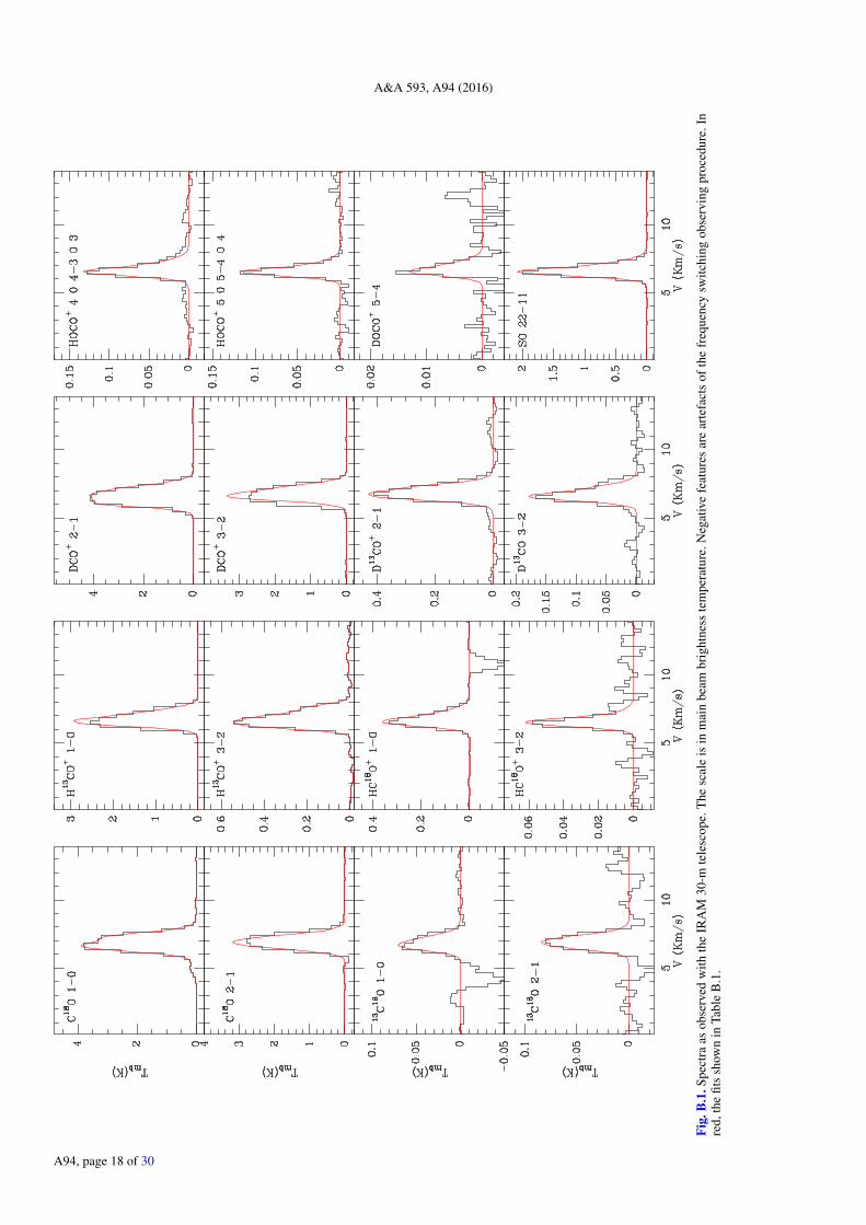
Fig.

B.1

.Spe

ctra

asob

serv

edw

ithth

eIR

AM

30-m

tele

scop

e.T

hesc

ale

isin

mai

nbe

ambr

ight

ness

tem

pera

ture

.Neg

ativ

efe

atur

esar

ear

tefa

cts

ofth

efr

eque

ncy

switc

hing

obse

rvin

gpr

oced

ure.

Inre

d,th

efit

ssh

own

inTa

ble

B.1

.

A94, page 18 of 30

A. Fuente et al.: Ionization fraction and the enhanced sulfur chemistry in Barnard 1

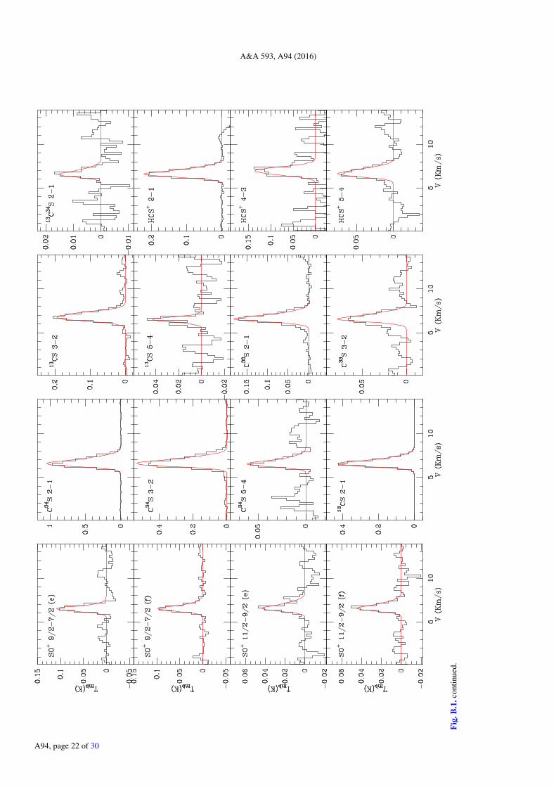
Fig.

B.1

.con

tinue

d.

A94, page 19 of 30

A&A 593, A94 (2016)

Fig.

B.1

.con

tinue

d.

A94, page 20 of 30

A. Fuente et al.: Ionization fraction and the enhanced sulfur chemistry in Barnard 1

Fig.

B.1

.con

tinue

d.

A94, page 21 of 30

A&A 593, A94 (2016)

Fig.

B.1

.con

tinue

d.

A94, page 22 of 30

A. Fuente et al.: Ionization fraction and the enhanced sulfur chemistry in Barnard 1

Fig.

B.1

.con

tinue

d.

A94, page 23 of 30

A&A 593, A94 (2016)

Fig.

B.1

.con

tinue

d.

A94, page 24 of 30

A. Fuente et al.: Ionization fraction and the enhanced sulfur chemistry in Barnard 1

Fig.

B.1

.con

tinue

d.

A94, page 25 of 30

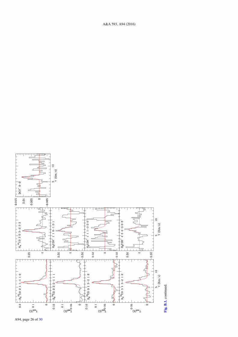
A&A 593, A94 (2016)

Fig.

B.1

.con

tinue

d.

A94, page 26 of 30

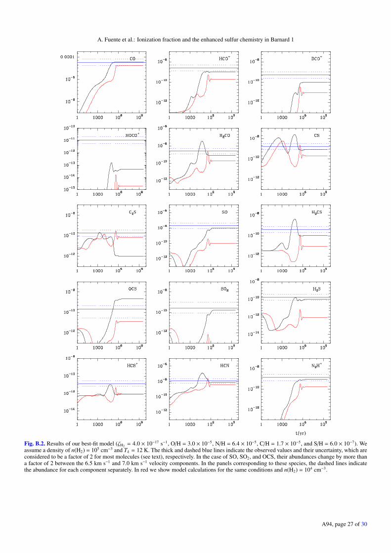
A. Fuente et al.: Ionization fraction and the enhanced sulfur chemistry in Barnard 1

Fig. B.2. Results of our best-fit model (ζH2 = 4.0 × 10−17 s−1, O/H = 3.0 × 10−5, N/H = 6.4 × 10−5, C/H = 1.7 × 10−5, and S/H = 6.0 × 10−7). Weassume a density of n(H2) = 105 cm−3 and Tk = 12 K. The thick and dashed blue lines indicate the observed values and their uncertainty, which areconsidered to be a factor of 2 for most molecules (see text), respectively. In the case of SO, SO2, and OCS, their abundances change by more thana factor of 2 between the 6.5 km s−1 and 7.0 km s−1 velocity components. In the panels corresponding to these species, the dashed lines indicatethe abundance for each component separately. In red we show model calculations for the same conditions and n(H2) = 104 cm−3.

A94, page 27 of 30

A&A 593, A94 (2016)

Fig. B.3. Results of our best-fit model (ζH2 = 4.0 × 10−17 s−1, O/H = 3.0 × 10−5, N/H = 6.4 × 10−5, C/H = 1.7 × 10−5, and S/H = 6.0 × 10−7). Weassume a density of n(H2) = 105 cm−3 and Tk = 12 K. The thick and dashed blue lines indicate the observed values and their uncertainties.

A94, page 28 of 30

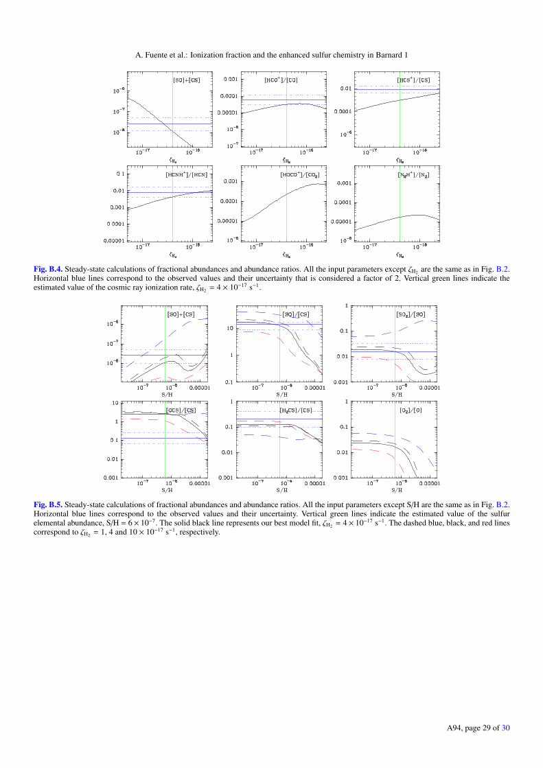
A. Fuente et al.: Ionization fraction and the enhanced sulfur chemistry in Barnard 1

Fig. B.4. Steady-state calculations of fractional abundances and abundance ratios. All the input parameters except ζH2 are the same as in Fig. B.2.Horizontal blue lines correspond to the observed values and their uncertainty that is considered a factor of 2. Vertical green lines indicate theestimated value of the cosmic ray ionization rate, ζH2 = 4 × 10−17 s−1.

Fig. B.5. Steady-state calculations of fractional abundances and abundance ratios. All the input parameters except S/H are the same as in Fig. B.2.Horizontal blue lines correspond to the observed values and their uncertainty. Vertical green lines indicate the estimated value of the sulfurelemental abundance, S/H = 6 × 10−7. The solid black line represents our best model fit, ζH2 = 4 × 10−17 s−1. The dashed blue, black, and red linescorrespond to ζH2 = 1, 4 and 10 × 10−17 s−1, respectively.

A94, page 29 of 30

A&A 593, A94 (2016)

Fig. B.6. Steady-state calculations of fractional abundances and abundance ratios. All the input parameters except O/H are the same as in Fig. B.2.Horizontal blue lines correspond to the observed values and their uncertainty. Vertical green lines indicate the estimated value of C/O elementalratio, C/O = 0.6. The dashed blue, black, and red lines correspond to ζH2 = 1, 4 and 10 × 10−17 s−1, respectively.

A94, page 30 of 30