IO in I-O: Size, Industrial Organization and the

Input-Output Network Make a Firm Structurally

Important ∗

Basile Grassi†

Bocconi University and IGIER

December 19, 2017 – Version 2.1

(First version: November 21, 2016)

[Latest Version]

Abstract

There is a growing literature suggesting that firm level productivity shocks can help under-

stand macroeconomic level outcomes. However, existing models are very restrictive regarding the

nature of competition within sector and its implication for the propagation of shocks across the

input-output (I-O) network. This paper offers a more comprehensive understanding of how firm

level shocks can shape aggregate dynamics. To this end, I build a tractable multi-sector heteroge-

neous firm general equilibrium model featuring oligopolistic competition and an I-O network. It

is shown that a positive shock to a large firm increases both the productivity and the markup at

the sector level. By reducing the sector price, the change in productivity propagates only to down-

stream sectors. Conversely, the change in markup, by increasing price and reducing demand for

intermediate inputs, propagates both to downstream and upstream sectors. The sensitivity of ag-

gregate output to firms’ shocks is determined by the sector’s (i) Herfindahl Index, which measures

the competition intensity of the sector, (ii) position in the input-output network, which measures

the direct and indirect importance of this sector for the household, and (iii) the profit share along

the supply chain, which relates to the changes in demand to upstream sectors.

Keywords: Oligopoly, Imperfect Competition, Input-Output Network, Industrial Organization,

Firm Heterogeneity, Random Growth, Granularity, Volatility, Micro-Origin of Aggregate Fluctua-

tions, Shocks Propagation, Production Network

∗I would like to acknowledge helpful comments from Axelle Arquié, James Best, Florin Bilbiie, Paul Beaudry, Ariel Burstein, Vasco M.Carvalho, Nuno Coimbra, Giancarlo Corsetti, Julian di Giovanni, Martin Ellison, Emmanuel Farhi, John Fernald, Jean Flemming, FrançoisFontaine, Xavier Gabaix, Christian Hellwig, Clément Imbert, Jean Imbs, Nir Jaimovich, Julien Labonne, Andrei A. Levchenko, FrancescoLippi, Ernest Liu, Isabelle Mejean, Ezra Oberfield, Franck Portier, Dan Quigley, Morten O. Ravn, Pontus Rendahl, Jean-Marc Robin, DavidRonayne, Vincent Sterk, Alireza Tahbaz-Salehi, and Andre Veiga. I would like to thanks seminar participants at the 2016 European WinterMeeting of the Econometric Society, Banque de France (Joint French Macro Workshop), Barcelona GSE Summer Forum (FGE), Bocconi,6th Annual Brandeis Summer Workshop, Bristol, Cambridge, Cornell, DEGIT 2017, EIEF, EUI, Essex, Harvard, INSEAD, Mannheim, Oxford,Paris School of Economics, Polytechnique, Sciences-Po, SED 2017, SUFE, Toulouse School of Economics, UCL, University of Oslo, Uni-versity of Wisconsin-Madison and the University of Zurich. I would also like to acknowledge support of the “Foscolo Top-Up Fellowship2015” from Unicredit and University.

†Bocconi University, Department of Economics, Via Rontgen 1, 20136 Milano, Italy. Email: basile.grassi@unibocconi.it

1 Introduction

Firm-level productivity shocks can explain an important part of movement in prices and output at

the sector and macroeconomic level1. The idea is that a handful of large firms represents a large

share of a sector, and thus shocks hitting these large firms cannot be balanced out by those affect-

ing smaller firms. However, typical models are very restrictive regarding the nature of competition

within a sector: firms are large enough to have a systemic importance but these firms do not inter-

nalized it when they make their decisions. This paper explores the alternative oligopolistic market

structure where firms do take into account the effect of their decisions on sector-level price and

quantity in order to study the propagation of firm-level shocks to other sectors through the Input-

Output (I-O) network. The properties of the propagation that arises under oligopolistic competition

are shown to be dramatically different from the monopolistic case both at the sector and macroeco-

nomic level.

Table 1 and Figure 1 motivate this paper: sectors are concentrated and linked through a “small

world” I-O network. Table 1 shows summary statistics of the top four firms’ share of industry rev-

enue in 2002, 2007 and 2012 for around 970 industries. Industry revenue accounted for by the top

four firms varies from almost zero to close to 100% with a median value close to 33% in 2007. The first

thing to note is that large firms represent an important share of revenue of the median sector. Sec-

ondly, as concentration is a widely used measure of a sector’s competition intensity, this table also

suggests that different sectors have different competition levels. For the bottom 25% of these sectors

the top four firms account for less than 18% of the total industry revenues, while for the top 25%

of theses sectors, only four firms account for more than 50% of the total industry revenues. While

confirming the “granular” nature of these sectors, this table emphasizes the heterogeneity across

sectors of the intensity of competition. Besides, these sectors are not independent from each other:

production in one sector relies on a complex and interlocking supply chain. Figure 1 displays the

I-O network among 389 sectors for the US in 2007. This is a “small world” network: a few nodes are

connected to many other nodes. In such production networks, as shown by Acemoglu et al. (2012),

Carvalho (2010, 2014) and Baqaee (2016), sector-level shocks translate into aggregate volatility. In

this paper, I study how firm-level shocks affect sector-level productivity and competition and how

these shocks propagate in the I-O network and thus shape the aggregate dynamics.

To this end, I build a tractable multi-sector heterogeneous firm general equilibrium model featuring

oligopolistic competition and an I-O network. Within each sector, a finite number of heterogeneous

firms are subject to oligopolistic competition and set variable markups à la Atkeson and Burstein

(2008). Up to an approximation, two sector-level sufficient statistics, the sum and Herfindahl index

of the firms’ productivity entirely characterize the equilibrium of this economy.

1An important paper in the growing literature on the micro-origin of aggregate fluctuations is the seminal work byGabaix (2011) where he shows that when the firm-size distribution is fat-tailed, firm-level shocks do not wash out at the

aggregate. Building on this seminal work, Carvalho and Grassi (2017) show that firm dynamic models contain a theory ofbusiness cycle as soon as the continuum of firms’ assumption is relaxed. Acemoglu et al. (2012), Carvalho (2010, 2014)and Baqaee (2016) build on the multi-sector business cycle framework of Long and Plosser (1983) to show how shocks onsectors linked through an I-O network can translate into aggregate fluctuations. Earlier contributions include Jovanovic

1

Figure 1: The US Input-Output Network in 2007

NOTE: Larger nodes of the network represent sectors supplying inputs to many other sectors. A darker color represents

higher top four firms’ share of total revenues in 2007 (sectors without available data are left white). There are 389 sectors.

Source: Bureau of Economic Analysis, detailed I-O table for 2007 and Census Bureau. The figure is drawn with the software

package Gephi.

2

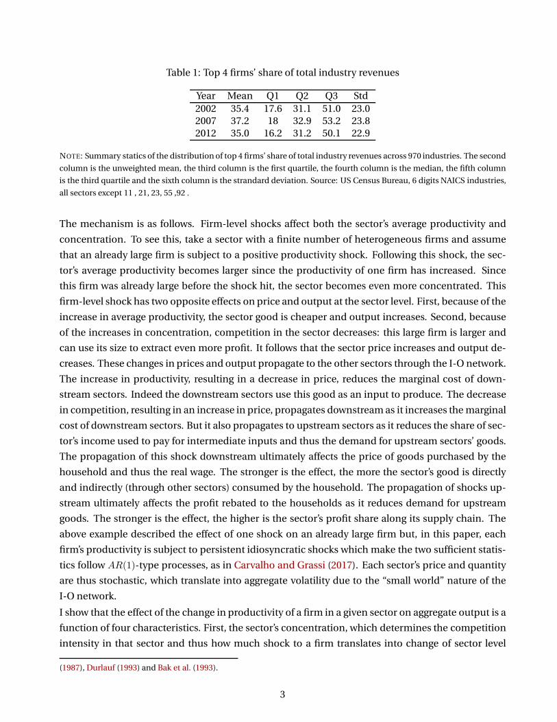
Table 1: Top 4 firms’ share of total industry revenues

Year Mean Q1 Q2 Q3 Std

2002 35.4 17.6 31.1 51.0 23.0

2007 37.2 18 32.9 53.2 23.8

2012 35.0 16.2 31.2 50.1 22.9

NOTE: Summary statics of the distribution of top 4 firms’ share of total industry revenues across 970 industries. The second

column is the unweighted mean, the third column is the first quartile, the fourth column is the median, the fifth column

is the third quartile and the sixth column is the strandard deviation. Source: US Census Bureau, 6 digits NAICS industries,

all sectors except 11 , 21, 23, 55 ,92 .

The mechanism is as follows. Firm-level shocks affect both the sector’s average productivity and

concentration. To see this, take a sector with a finite number of heterogeneous firms and assume

that an already large firm is subject to a positive productivity shock. Following this shock, the sec-

tor’s average productivity becomes larger since the productivity of one firm has increased. Since

this firm was already large before the shock hit, the sector becomes even more concentrated. This

firm-level shock has two opposite effects on price and output at the sector level. First, because of the

increase in average productivity, the sector good is cheaper and output increases. Second, because

of the increases in concentration, competition in the sector decreases: this large firm is larger and

can use its size to extract even more profit. It follows that the sector price increases and output de-

creases. These changes in prices and output propagate to the other sectors through the I-O network.

The increase in productivity, resulting in a decrease in price, reduces the marginal cost of down-

stream sectors. Indeed the downstream sectors use this good as an input to produce. The decrease

in competition, resulting in an increase in price, propagates downstream as it increases the marginal

cost of downstream sectors. But it also propagates to upstream sectors as it reduces the share of sec-

tor’s income used to pay for intermediate inputs and thus the demand for upstream sectors’ goods.

The propagation of this shock downstream ultimately affects the price of goods purchased by the

household and thus the real wage. The stronger is the effect, the more the sector’s good is directly

and indirectly (through other sectors) consumed by the household. The propagation of shocks up-

stream ultimately affects the profit rebated to the households as it reduces demand for upstream

goods. The stronger is the effect, the higher is the sector’s profit share along its supply chain. The

above example described the effect of one shock on an already large firm but, in this paper, each

firm’s productivity is subject to persistent idiosyncratic shocks which make the two sufficient statis-

tics follow AR(1)-type processes, as in Carvalho and Grassi (2017). Each sector’s price and quantity

are thus stochastic, which translate into aggregate volatility due to the “small world” nature of the

I-O network.

I show that the effect of the change in productivity of a firm in a given sector on aggregate output is a

function of four characteristics. First, the sector’s concentration, which determines the competition

intensity in that sector and thus how much shock to a firm translates into change of sector level

(1987), Durlauf (1993) and Bak et al. (1993).

3

markup and price. Second, the sector centrality, which measures that sector’s direct and indirect

importance in the household’s consumption bundle. This characteristic relates to the transmission

of firm-level shocks to downstream sectors. Third, the sector’s profit share over its whole supply

chain, which measures how much profit is captured directly and indirectly (through the I-O network)

by that sector. This characteristic relates to the propagation of firm level shocks to upstream sectors.

Finally, the firm size which interacts with these characteristic and determines the strength of the

downstream and upstream propagation.

Furthermore, I show that a change in productivity of a firm in a given sector propagates to price of

downstream sectors and to sales share of upstream sectors. Because of oligopolistic competition,

a change in productivity of one firm does not pass through fully on sector-level price while chang-

ing the profit and cost share. The change in price propagates to downstream sectors but is either

reduced or magnified, relative to the monopolistic competition case, depending on the identity of

the firm subject to the shock. The change in profit and thus cost share propagates to upstream sec-

tors and affects their sales as a share of output. The latter mechanism requires both oligopolistic

competition and an I-O network.

Thanks to the high tractability of the model and the fact that the equilibrium is characterized by

two sector-level sufficient statistics, I calibrate this economy by relying on the choice of a few deep

parameters, the Census’ concentration data that pin downs sectors’ competition intensity and the

Bureau of Economic Analysis (BEA)’s Input-Output data. For the benchmark calibration, the out-

put volatility that comes out of simulated data is 34% of what is observed in the data. Furthermore,

thanks to the high tractability of the model, I decompose the aggregate volatility in the contribution

of the “downstream” and “upstream” effect. The “downstream” effect contributes to 89%, the “up-

stream” to 1.3% and the remaining 9.64% are due to the covariance. In a version of this model with

monopolistic competition rather than oligopolistic competition all the aggregate volatility is due to

the “downstream” effect.

Related Literature: This paper contributes to the literature on the micro-origin of aggregate fluc-

tuations. This literature is based on two mains ideas: the “granular hypothesis” and the network

origin. For the former, seminal work by Gabaix (2011) shows that whenever the firm-size distribu-

tion is fat-tailed, idiosyncratic shocks do not average out quickly enough and therefore translate

into sizable aggregate fluctuations. Carvalho and Grassi (2017) ground the “granular hypothesis” in

a well-specified firm dynamic setup. For the latter, Acemoglu et al. (2012) and Carvalho (2010) show

that when the distribution of sectors’ centrality in the I-O network is fat tailed then sector level per-

turbations also generate sizable aggregate fluctuations. Relative to these papers, I present the first

framework that includes both components explicitly. The “granular hypothesis” leads to sector-level

fluctuations whereas the I-O network structure translates sector-level fluctuations into aggregate

fluctuations.2 An important drawback of this literature is that firms are supposed to be large enough

to influence the aggregate but also small enough not to be strategic. In Carvalho and Grassi (2017)

2Notable contribution in this literature include but are not limited to di Giovanni et al. (2014), Magerman et al. (2016)and Baqaee and Farhi (2017a).

4

framework such assumptions were made because firms interacted in a perfectly competitive labor

market. Here, I present the first model of strategic pricing where aggregate fluctuations arise from

purely idiosyncratic shocks. When they are taking their decisions, firms do take into account the fact

that they have market power and can influence their sector’s output and price.

Recently, Baqaee and Farhi (2017a) revisit the famous and influential result by Hulten (1978) which

states that for efficient economies the first order impact of a productivity shock to a firm on aggre-

gate output is equal to that firm’s sales as a share of output. The framework presented here is not

subject to this result as the economy is not efficient. Therefore it is closer to Basu (1995), Basu and

Fernald (2002), Jones (2011, 2013), Bigio and La’O (2016) or Baqaee and Farhi (2017b) who study the

introduction of distortions in multi-sector macroeconomic model with production networks. Con-

trary to all of these papers, here, firm level productivity shocks endogenously affect markups, the

distortions in this economy.

An important and growing literature studies the transmission of shocks across sectors through the

I-O network: Acemoglu et al. (2015) look at the transmission of well identified supply and demand

shocks, Carvalho et al. (2016) and Boehm et al. (2016) study the firm level impact of supply chain

disruptions occurring in the aftermath of the Great East Japan Earthquake in 2011, while Barrot and

Sauvagnat (2016) look at the effect of natural disasters. Baqaee (2016) studies theoretically the ef-

fect of shocks on entry cost. In this paper I introduce a new propagation mechanism of firm-level

shocks in the I-O network through change in sector-level competition, which act as supply shocks

to downstream sectors and demand shocks to upstream sectors. Firm-level shocks propagate both

downstream and upstream despite the Cobb-Douglas assumption, furthermore firm size affects the

sign of the upstream propagation.

This paper also contributes to the literature on imperfect competition among heterogeneous firms.

Krugman (1979), Ottaviano et al. (2002), Melitz and Ottaviano (2008), Bilbiie et al. (2012) and Zhelo-

bodko et al. (2012) study demand-side pricing complementary whereas I look at supply-side pricing

complementaries as in Atkeson and Burstein (2008) but in an I-O context. Furthermore I show, up

to an approximation, that such a model is highly tractable and that firm heterogeneity can be sum-

marized at the sector level by just two sufficient statistics.

Finally, this paper relates to a recent and growing empirical literature that documents and analy-

ses the macroeconomic consequences of the rise in market concentration in the US. Barkai (2017),

Autor et al. (2017) and Kehrig and Vincent (2017) explain the secular declines in labor share from

the increase of sector level and firm level concentration, while Loecker and Eeckhout (2017) docu-

ment an increase in firm level markup which they relate to a number of secular trends in the last

three decades. Even if the focus of this paper is different, it contributes to this literature by providing

a simple and tractable model to analyze the aggregate consequence of market concentration. For

example, market concentration is shown here to be driving sector-level markup and therefore the

profit and labor share.

Outline: The paper is organized as follows. In Section 2, I describe and solve the household’s and

firm’s problem. In Section 3, I first aggregate firms’ behavior at the sector level and show that firm

5

heterogeneity can be summarized by two sufficient statistics. I then solve for the dynamics of these

two statistics. In Section 4, I show that a firm’s sector market structure, its role in the input-output

network and the firm’s size jointly determine its structural importance. In Section 5, I look at how

firm-level productivity shocks propagate to other sectors through the I-O network. In Section 6, I

calibrate the model and perform some quantitative exercises. Finally, Section 7 concludes.

2 Model

In this section, I describe the structure of the economy and I solve for the household and firms’

problem. There are two types of agent. First, a representative household consumes and supplies

labor. Second, there is a finite number of firms distributed across a finite number of sectors that are

linked by a production network. In each sector, firms set their price (or quantity) strategically. Each

firm is subject to independent persistent idiosyncratic shocks independent.

2.1 Household

The representative household lives a discrete and infinite number of periods. Preferences are given

by E0∑∞

t=0 ρtu(Ct, Lt) where u(Ct, Lt) is the instantaneous utility, ρ is the discounted rate, Ct is the

composite consumption good, and, Lt is the number of hours worked at time t.

The composite consumption good Ct is a Cobb-Douglas aggregation of N ∈ N sector-level goods:

Ct = θ∏N

k=1Cβk

k,t whereCk,t is the amount of good k consumed by the household at time t and where

θ is a normalization constant.3 The Cobb-Douglas weights, βk, are equal to the expenditure shares of

each goodPk,tCk,t

PCt Ct

where Pk,t is the price of good k andPCt is the aggregate price index which satisfies

PCt =

∏Nk=1 P

βk

k,t . Note that N is an integer number.

In a sector k, there is an integer number, Nk, of varieties index by i. These varieties are aggregated

with a constant elasticity of substitution εk > 1 such that Ck,t =(∑Nk

i=0 Ct(k, i)εk−1

εk

) εkεk−1

where

Ct(k, i) is the amount of sector k’s variety i consumed by the household at time t. Finally, the price of

good k satisfiesPk,t =(∑Nk

i=1 Pt(k, i)1−εk

) 1

1−εk where Pt(k, i) is the price of variety i in sector k at time

t. Each variety is produced by exactly one firm, and all the firms are owned by the representative

household.

The above household preferences and the assumption that εk > 1 capture the idea that as one is

dissagregating further, from sectors to firms, it is easier for the household to substitute between

two dissagregating units. Furthermore, the degree of substitution between two varieties of the same

good is higher that between two varieties of two different goods.

3The normalization constant θ makes the mathematics simpler and is equal to θ =∏N

k=1 β−βkk .

6

2.2 Firms

An integer number of firms are splited inN sectors. In sector k, there areNk firms and each variety is

produced by exactly one firm. Firms are heterogeneous in their (labor-augmenting) productivity. A

sector is defined as a technology and a market structure: (i) firms in the same sector have access to

the same production function (ii) these firms compete with each other in a differentiated Bertrand

or Cournot game. At the end of this section, I show that the implied firm dynamics in this model is

consistent with recent empirical evidences.

Technology: The firm i in sector k combines labor, Lt(k, i), and other sectors’ goods, xt(k, i, l), to

produces yt(k, i) units of its variety using the constant return to scale Cobb-Douglas technology

yt(k, i) = αk

(Zt(k, i)Lt(k, i)

)γk ∏Nl=1 xt(k, i, l)

ωk,l where γk is the labor share in the production, αk

is a normalization constant,4 Zt(k, i) is the labor-augmenting productivity specific to the firm i in

sector k, ωk,l is the input share of sector l’s goods needed in sector k’s production. The (N ×N) ma-

trix Ω = ωk,lk,l represents the input-output network.5 Thanks to constant return to scale the kth

rows of Ω sum to 1−γk:∑N

l=1 ωk,l = 1−γk. Furthermore, xt(k, i, l) is a composite of sector l’s varieties

such that xt(k, i, l) =(∑Nl

j=1 xt(k, i, l, j)εl−1

εl

) εlεl−1

where xt(k, i, l, j) is the quantity of the variety j of

sector l’s good that is used for the production of variety i of sector k’s good. Note that the elasticity

of substitution among varieties in a sector is the same for firms and for the household.

The input-output network Ω is assumed to be fixed across time and state because it is a sector-level

network. Here the input-output linkages are interpreted as technology: the input bundle needed

to produce the variety of a good. At the business cycle frequency, this technology is not affected by

labor-augmenting firm-level productivity shocks that are considered here. However, if one firm in a

sector increases massively the price of its variety, its customers are able to substitute away from this

variety thanks to the double-nested constant elasticity of substitution demand system. Therefore

even if the sector-level input-output linkages are fixed, the transaction network between firms is not

and varies across time and state.6

The productivity of firm i in sector k, Zt(k, i), is identically and independently distributed across

firms but not across time. It follows a sector specific Markov chain over the discrete state spaceΦk =

1, ϕk , ϕ2k, · · · , ϕn

k , · · · , ϕMk

k = ϕnkn∈0,1,...,Mk for ϕk > 1 which is evenly distributed in logs.7 This

Markov chain is described by the matrix of transition probabilities P(k) = P(k)n,n′n,n′ where P(k)

n,n′ =

P(Zt+1(k, i) = ϕn′

k |Zt(k, i) = ϕnk

)is the probability that a firm i in sector k jumps from productivity

level ϕnk to ϕn′

k between time t and time t + 1. In some cases, I assume a specific Markovian chain

which is a discretization of a random growth process and is taken from Córdoba (2008). Figure 2 and

4The normalization constant αk makes the mathematics simpler and is equal to αk = γ−γkk

∏Nl=1 ω

−ωk,l

k,l .5The notation U = uk,lk,l means that U is the matrix where the element k, l is equal to uk,l, while I denote v = vkk

the vector where the element k equal to vk .6This differs from Magerman et al. (2016) who study the micro-origin of firm-level shocks in a fixed firm-to-firm trans-

action network.7This means that ϕn+1

k /ϕnk = ϕk.

7

Figure 2: Productivity Process

nt,k,int,k,i − 1 nt,k,i + 1

ak

bk = 1− ak − ck

ck

NOTE: A representation of the transition probabilities in assumption 1 of a firm i in sector k for Mk > nt,k,i > 0.

Assumption 1 describe its transition probabilities.

Assumption 1 (Random Growth) For ak + bk + ck = 1, firm level productivity in sector k follows a

Markov chain over Φk = ϕnkn∈0,1,...,Mk with transition probabilities such that:

P(k) =

ak + bk ck 0 · · · · · · 0 0

ak bk ck · · · · · · 0 0

· · · · · · · · · · · · · · · · · · · · ·

0 0 0 · · · ak bk ck

0 0 0 · · · 0 ak bk + ck

Pricing: A sector is also defined as a market where firms are engaged in imperfect competition.

Sector’s goods are imperfect substitute and varieties within a sector are more substitutable: εk > 1.

Each firm produce exactly one variety of its sector’s good and customers cannot perfectly substitute

between two varieties: εk < ∞. Following Atkeson and Burstein (2008), I assume that firms play a

static game where firm i in sector k chooses its price Pt(k, i) taking as given the prices chosen by

other firms in the economy, the other sectors’ price and quantities, the wage, and, aggregate prices

and quantities. Importantly note that this firm does recognized that sector k’s price and quantity is

affected when it changes its price.

To understand this assumption, let us imagine that General Motors (GM) has a way to produce a car

that cost $10000 less than its competitors. The above assumption implies that, when GM is taking

its pricing decision, it is internalizing the impact of its decision on the quantity and price of the

“Automobile Manufacturing” sector but not on the “Amusement Parks and Arcades” sector. Note

that with these assumptions in place, GM is not internalizing the impact of its pricing decision on

the real wage and on the prices and quantities of its upstream or downstream sectors. Relaxing

these assumptions might create effects that will go beyond the scope of this paper and I leave these

questions for future research.8

8Another interpretation of the assumptions made here is that firms have limited ability to compute the effect of theirdecision on any variable outside their sector’s price and quantity. This is fundamentally different from the Atkeson andBurstein (2008) framework because, in their paper, they assume a continuum of sectors: even if firms are not atomisticwithin a sector, a firm’s sector is atomistic with respect to the aggregate economy.

8

Note that here I assume a competition in price (labeled as Bertrand). In most of the results below, I

compare the baseline case of Bertrand competition with (i) the case of Cournot competition where

firms compete in quantity and (ii) with the benchmark case of monopolistic Dixit and Stiglitz (1977)

competition. When it does not create confusions, I abstract from the time t subscript.

As a result of cost-minimization, firm i in sector k face a marginal cost λ(k, i) =

Z(k, i)−γkwγk∏N

l=1 Pωk,l

l where w is the wage rate in this economy. Note that due to the presence of

input-output linkages, this marginal cost is a function of other sectors’ prices. The sector level gross

output is defined as Yk =(∑Nk

i y(k, i)εk−1

εk

) εkεk−1

. Proposition 1 characterizes the pricing decision of

a firm i in sector k.

Proposition 1 (Firm’s Pricing) The firm i in sector k sets a price P (k, i), a markup µ(k, i) and has a

sale share s(k, i) that satisfy the following system of equations:

P (k, i) = µ(k, i)λ(k, i)

s(k, i) =P (k, i)y(k, i)

PkYk=

(P (k, i)

Pk

)1−εk

µ(k, i) =

εkεk−1 Under Monopolistic Competitionεk−(εk−1)s(k,i)

εk−1−(εk−1)s(k,i) Under Bertrand Competitionεk

εk−1−(εk−1)s(k,i) Under Cournot Competition

Proof See Atkeson and Burstein (2008).

The first thing to note in the above proposition is that firms charge a markup over their marginal

cost. Under monopolistic Dixit and Stiglitz (1977) competition the markup is constant and equal to

εk/(εk − 1). Under oligopolistic competition (Bertrand or Cournot), the markup charged is increas-

ing in the sales share of the firm: larger firms charge a higher markup.

Note that in both the Bertrand and Cournot competition case, the markup charged by a firm is con-

verging to a constant as the size of this firm goes to zero. Indeed, for firm i in sector k, we have

µ(k, i) → εk/(εk − 1) as s(k, i) → 0. As a firm gets atomistic, its markup is getting closer to the one

under monopolistic competition. Because the system of equation in Proposition 1 does not admit

an analytical solution, aggregating firms’ behavior at the sector level in a tractable way turns out

to be impossible. To circumvent this issue, Proposition 2 is approximating the sales share of a firm

under oligopolistic competition by the sales share of this firm under monopolistic competition. In

Section 3, this result is used to collapse firms’ heterogeneity to two sector-level statistics.

Proposition 2 (Firm’s Approximation) The sales share of firm i in sector k under monopolistic com-

petition is a function of its marginal cost λ(k, i) and the sector k price index: s(k, i) =(

εkεk−1

λ(k,i)Pk

)1−εk.

When s(k, i) → 0, the sales share of this firm under oligopolistic competition, s(k, i), satisfies

s(k, i) =

s(k, i)−(1− ε−1

k

)s(k, i)2 + o

(s(k, i)2

)Under Bertrand Competition

s(k, i)− (εk − 1) s(k, i)2 + o(s(k, i)2

)Under Cournot Competition

where the notation f(x) = o(g(x)

)means f(x)/g(x) → 0 when x→ 0.

9

Proof See Appendix A.1.

In this proposition, the sales share of firm i in sector k is approximated by the sales share under

monopolistic competition s(k, i). Since there is a one to one mapping between the marginal cost

and s(k, i) for a fixed sector price index Pk, one can think of this result as a approximation of the

sales share of firms by a function of their marginal cost. Similarly, the above results holds when

s(k, i) is small or, since εk > 1, when the marginal cost λ(k, i) is large.

Figure 3: Approximation of Firms’ Sales Share

0 0.05 0.1 0.15 0.2

Sales Share

0

0.02

0.04

0.06

0.08

0.1

0.12

0.14

0.16

0.18

SalesShare

Bertrand

Approx 2nd

Approx 3rd

0 0.05 0.1 0.15 0.2

Sales Share

0

0.5

1

1.5

2

2.5

Deviation

NOTE: For εk = 5. The left panel shows the Bertrand sales share using a numerical solver, the second and the third

order approximation as a function of the monopolistic sales share. The right panel shows percentage deviation of both

approximations with respect to the numerical solution.

The framework derived in this paper is designed to capture the aggregate effect of shocks on “large”

firms while the results in Proposition 2 holds for “small” firms in their market. Therefore, it is impor-

tant to know if “small” in the sense of the approximation in Proposition 2 is “small” economically.

Figure 3 displays on the left panel the sales share under Bertrand competition as a function of the

sales share under monopolistic competition along with the second and third order approximation.

The right panel of this figure displays percentage deviations of the approximations with respect to

the exact solution. For sales share up to 20%, the error made by the second order approximation

is less than 1.5%: “small” for the approximation in Proposition 2 is thus not small economically. In

order to aggregate the firms behavior at the sector level, in some cases, I assume this approximation

to hold. 9, 10

9For conciseness, the third order approximation is not reported in the formula in Proposition 2 but can be found in theproof of this proposition in Appendix A.1.

10A concern could be that this approximation holds well only in levels and not in term of slopes. Figure 10 in OnlineAppendix E shows that for sales share up to 20%, the error made on the slope is less than 5%. An other concern might bethe quality of this approximation depends on the value of the elasticity across varieties in a sector εk. Figures 11 and 12 inOnline Appendix E shows that the quality of the approximation is of the same order for different values of εk.

10

Assumption 2 (Approximation) In Proposition 2’s approximation, higher order terms are negligible

Firm Dynamics: To conclude the description of the model, let us look at its implication in term

of firm dynamics. Under Assumption 1, the productivity of a given firm satisfies Gibrat’s law: the

growth rate is independent of the level. Especially, the level of productivity does not affect the mean

and the volatility of its growth rate. However, here Gibrat’s law is violated for a firm’s sales: larger

is a firm, larger is its market power and less sensitive are its sales to a change in its marginal cost.

Indeed, the firm’s level markup adjusts and thus the pass-through of shock to price is incomplete.

Proposition 3 shows this in a formal way.11

Proposition 3 (Size-Volatility) Under Assumption 1 and 2, the (conditional) variance of the growth

rate of firm i in sector k’s productivity and sales share satisfies:

Vart

[Zt+1(k, i) − Zt(k, i)

Zt(k, i)

]= σ2k and Vart

[st+1(k, i) − st(k, i)

st(k, i)

]= gk(st(k, i))σ

2k

where σ2k = a(ϕ−1k − 1

)2+ c (ϕk − 1)2 − (aϕ−1

k + b + cϕk − 1)2 and gk : x 7→ gk(x) is a decreasing

function. Furthermore, the slope of gk is increasing in εk.

Proof See Online Appendix F.1.

It is a well established fact that larger firms tends to be less volatile. Recently, Yeh (2017) explores

empirically the possible mechanisms that could give rise to such negative relationship between size

and volatility at the firm level. After ruling out diversification among establishments or products, he

concludes that large firms face smaller price elasticities and therefore respond less to a given-sized

productivity shock than small firms do. In the current framework, the reason behind the negative

size-volatility relationship of Proposition 3 is exactly the one identified by Yeh (2017).12

The simple demand system and the market structure assumed here together with the random

growth process for productivity implies a rich and empirically relevant firm dynamics. As it is shown

in the rest of this paper, non-negligible sector-level and aggregate fluctuations arise from firm-level

productivity shocks despite the fact that larger firm are less volatility.

3 Sectors Aggregation

The model derived above describes an economy where a finite number of firms, subject to produc-

tivity shocks, evolve and compete in their sector. The behavior and the dynamics of these firms

shape the sector-level variables. This section characterizes the mapping between firm-level and

sector-level variables. It shows that the latter are related to a few moments of the distribution of

firms whose dynamics is solve for.

11Gibrat’s law was first introduce by Gibrat (1931). See also Sutton (1997) for a review.12Empirical studies that identified a negative size-volatility relationship at the firm level are Comin and Philippon (2006)

and Comin and Mulani (2006) for publicly listed US firms, Fort et al. (2013) and Foster et al. (2008) for US manufacturingfirms, and di Giovanni et al. (2014) using a census of French firms.

11

This section is organized as follow. First, I introduce two key sector-level statistics. Second, I derive

the relationship between sector level markup and concentration before described the equilibrium

under Assumption 2. Finally, I describe the sector dynamics under Assumptions 1 and 2.

3.1 Two Statistics

In the model described in Section 2, given the distribution of productivity Zt(k, i) at each time t, one

can solve for the equilibrium allocation. The distributions of productivity in each sector are the state

variables of this economy. Let me introduce two moments of these distributions that turn out to be

key to describe the equilibrium allocation under Assumption 2.

For a given sector k, the first statistic is the sum of the productivity of sector k’s firms raise at a power

that take into account the downward slopping demand and the decreasing return in labor:

Zt,k =

Nk∑

i=1

Zt(k, i)(εk−1)γk

This statistic is proportional to the unweighted average of firm-level productivity (raised at a power)

in sector k and is therefore related to the first moment of the firm’s productivity distribution in that

sector. Note that in sector k, there is an integer number of firms Nk therefore when the productivity

of one firm changes this finite sum of productivity changes. More precisely, the elasticity of Zt,k with

respect to the productivity of firm i in sector k is ∂ logZk

∂ logZ(k,i) = (εk − 1)γkZ(k,i)(εk−1)γk

Zk> 0. If there was a

continuum of firms rather than an integer number then this elasticity would always be zero.

The second statistic is related to the second moment of the firms’ productivity distribution in sector

k. It is the sum of the square of firms’ productivity shares in Zt,k: the Herfindahl index of productivi-

ties in sector k:

∆t,k =

Nk∑

i=1

(Zt(k, i)

(εk−1)γk

Zt,k

)2

This statistic captures the dispersion of productivity across firms in a sector. The Herfindahl index

is a widely used measure of concentration. Note that this Herfindahl index is among firm level pro-

ductivity and therefore not directly observable. Because of the finite number of firms in sector k,

when the productivity of firm i in sector k changes then the concentration measure ∆t,k changes

too: ∂ log∆k

∂ logZ(k,i) = 2∆k

(Z(k,i)(εk−1)γk

Zk−∆k

)∂ logZk

∂ logZ(k,i) . Note that the elasticity of ∆t,k with respect to

Z(k, i) can be positive or negative depending on the productivity level of firm i in sector k relative

to the concentration measure ∆t,k. This is very intuitive, because when the productivity of a “large”

firm increases, i.e forZ(k,i)(εk−1)γk

Zk> ∆k, the concentration of productivity increases. Conversely,

when the productivity of a “small” firm increases, i.e forZ(k,i)(εk−1)γk

Zk< ∆k, the concentration of

productivity decreases.

Before describing the dynamics of these statistics under Assumption 1, I show that these two statis-

tics are sufficient to characterize the equilibrium allocation under Assumption 2.

12

3.2 Sector’s Allocation

In this subsection, I solve for the sector-level allocation. I start by defining the sector-level markup

and productivity before characterizing the sector-level allocation under Assumption 2. Since firms’

decisions are static, I abstract from the time t subscript in this section.

Markup: An important variable is the sector-level markup. This markup is defined as the sector-

level price divided by the sector-level marginal cost. For a given sector k, the marginal cost is defined

as λk = dTCk

dYkwhere TCk is the total cost in sector k: TCk =

∑Nk

i=1 λ(k, i)y(k, i). Note that in the context

of constant return to scale the marginal cost is also equal to the average cost therefore λk = TCk

Yk=

∑Nk

i=1 λ(k, i)y(k,i)Yk

. After using the fact that firm-level price is a markup over the marginal cost, it is

easy to see that the sector-level markup µk is

µk =Pk

λk=

(Nk∑

i=1

µ(k, i)−1s(k, i)

)−1

(1)

The sector’s markup is a sales share weighted harmonic average of firm level markups. This expres-

sion is valid as long as firms charge a markup over the marginal cost. It therefore applies to any of

the market structure assumed here: monopolistic, Bertrand and Cournot.

Proposition 4 shows that the sector-level markup is a function of sector-level concentration index.

Especially, the directly observable Herfindahl-Hirchman-Index (HHI), the sum of the sales share

squared, plays an important role.

Proposition 4 (Sector Level Markup) The sector k’s markup is equal to

µk =

εkεk−1 Under Monopolistic competition

εkεk−1

(1− 1

εk−1

∑∞m=2

(εk−1εk

)m−1(HKk(m))m

)−1

Under Bertrand competition

εkεk−1 (1−HHIk)

−1 Under Cournot competition

where HHIk =(∑Nk

i=1 s(k, i)2)

is the sector k’s Herfindahl-Hirchman-Index (HHI), and HKk(m) =(∑Nk

i=1 s(k, i)m)1/m

is the Hannah and Kay (1977) concentration index. NB: HKk(2)2 = HHIk the

HHI is the square of the second Hannah and Kay (1977) concentration index.

Proof See Appendix A.2.

The above proposition shows that under monopolistic competition the sector-level markup is con-

stant and equal to the firm-level markup. This is obvious since the sector’s markup is an average

of firms’ markups and under monopolistic competition all the firms in a given sector charge the

same markup. As soon as pricing becomes strategic, under Bertrand or Cournot competition, the

sales share distribution in the sector plays a crucial role. Under Cournot competition for example,

the Herfindahl-Hirchman-Index entirely determines the sector’s markup. The intuition is as follows,

13

when the sector’s concentration is high, i.e the Herfindahl-Hirchman-Index is high, large firms have

a higher market share and thus they can use this higher market power to charge higher markups

which in turn aggregate to a higher sector’s markup. An important implication of Proposition 4 is

that it links empirically observable variables, such as the Herfindahl-Hirchman-Index, to the sector

level markup.

Using the result in the above proposition, it is easy to derive some comparative statics of the markup

with respect to the Herfindahl-Hirchman-Index while keeping everything else constant.

∂µk∂HHIk

=

0 Under Monopolistic competitionεk−1ε2k

µ2k > 0 Under Bertrand competitionεk−1εk

µ2k > 0 Under Cournot competition

Under Bertrand and Cournot competition, a higher sector’s Herfindahl-Hirchman-Index always im-

plies a higher sector’s markup. This relationship is stronger for low competitive, high markup sectors.

The sensitivity of the sector’s markup to the sector’s Herfindahl-Hirchman Index is stronger under

Cournot than under Bertrand competition. In this framework, given the demand system and the

assumed market structure, sector concentration is a measure of sector competition.

Productivity: The other important variable to define is the sector-level productivity. This is de-

fined as the sector-level labor-augmenting productivity. As it was shown above, the sector-level

marginal cost is λk =∑Nk

i=1 λ(k, i)y(k,i)Yk

. After substituting for the firm-level marginal cost λ(k, i) =

Z(k, i)−γkwγk∏N

l=1 Pωk,l

l , the sector-level marginal cost is equal to λk = Z−γk

k wγk∏N

l=1 Pωk,l

l where

Z−γk

k =

Nk∑

i=1

Z(k, i)−γky(k, i)

Yk

is the sector k’s (labor-augmenting) productivity, an output weighted sum of firm-level productivity

in sector k. It is entirely determined by the joint distribution of output and productivities across

firms in a sector, while the sector-level markup was entirely determined by the distribution of sales

share.

Allocation: The previous results were relating endogenous variables with each other and were not

linking equilibrium allocation to the state variable in this economy. Proposition 5 first solves for the

sector allocation given the sectors’ markup and productivity, before explicitly describing how the

14

two statistics Zk and ∆k entirely characterize the sector-level variables under Assumption 2.

Proposition 5 (Sector Allocation) Sectors’ prices are equal to:

log Pkk = (I −Ω)−1

log µl

(w

Zl

)γl

l

(2)

where the (N × N)-matrix Ω is such that Ω = ωk,l1≤k,l≤N and I is the (N × N)- identity matrix.

Sectors’ sales share are equal to: PkYkPCC

′

k

= β′(I − Ω)−1 (3)

where the (N ×N)-matrix Ω is such that Ω = µ−1k ωk,l1≤k,l≤N and the (N × 1)- vector β is such that

β = βkk. Under Assumption 2, sector k’s markup and productivity are equal to:

µk =εk

εk − fk (∆k)and Zk =

(Zk

) 1

γk(εk−1)

(fk (∆k)

) −1

γk(εk−1)

(εk − fk (∆k)

εk − 1

)−1

γk

where

fk(x) =

1 Under Monopolistic Competition

1−√

1−4(1−ε−1k )x

2(1−ε−1k )x

for x ∈[0, 1

4(1−ε−1k )

]Under Bertrand Competition

1−√

1−4(εk−1)x

2(εk−1)x for x ∈[0, 1

4(εk−1)

]under Cournot Competition

Proof See Appendix A.3.

The above proposition characterizes the sectors’ allocation for a given wage w. The System 2 of N

equations relates the sectors’ prices with sectors’ productivities Zl, sectors’ markups µl, wage w and

the input-output matrix Ω. To understand these equations, let us assume that there is no input-

output linkages, i.e Ω = 0 and γk = 1. In this case the price in sector k is just the sector’s markup µk

over the marginal cost in this sector (w/Zk)γk , which is standard under imperfect competition. Now

let us assume that the input-output structure is the one described in Figure 4, i.e sector k is using

labor and sector l’ good to produce, while sector l is using only labor as input. Under imperfect

competition, the price in sector k is equal to the sector’s markup µk over the marginal cost. However,

the sector k’s marginal cost is(

wZk

)γk

(Pl)ωk,l , a combination of the marginal cost of labor and the

price of the upstream sector l’s good. The sector l’s price is itself equal to the markup in sector l over

the marginal cost of labor in sector l: Pl = µl

(wZl

). To solve for the prices of sector k and l, one just

need to solve a system of two unknowns and two equations. The System 2 is a generalization of this

reasoning for any input-output network Ω.13

The System 3 ofN equations solves for the sectors’ sales share as a function of the household expen-

diture share β, the markups and the input-output network through Ω. To understand the intuition

13For the case of perfect competition, i.e for µk = 1, an implication of the system of Equations 2 is that the sector’s priceis equal to the marginal cost of labor used directly and indirectly, through the input-output network.

15

Figure 4: A Simple Input-Output Structure

lk

ωk,l

NOTE: In this simple input-output structure, firms in sector k are using labor and sector l’s good to produce their variety,

while firms in sector l are using only labor.

behind this matrix, let us assume that the input-output structure is the one described in Figure 4 and

let us compute the income share that sector l captures from a dollar spend on sector k’s good. Some

of that dollar, a share 1−µ−1k , is rebated directly as profit to the household by sector k, the remaining

is used to pay for inputs among which sector l’s good. Therefore, sector l receives a share µ−1k ωk,l of

this dollar. For any input-output network, the element (k, l) of the matrix Ω is the share of income

that flows directly from sector k to sector l and is equal to µ−1k ωk,l. Equations 3 shows that the sales

share of a sector is given by the vector β′(I− Ω)−1 = β′+β′Ω+β′Ω2+ . . .which captures the fact that

the total sales of a sector is the sum of the direct and indirect sales to the household. A given sector

receives income directly from the sales to the household. This is captured by the term β′ in Equa-

tions 3. In addition, this sector’s good is also sold to its downstream sectors that used it as inputs

and serve the household. This first-degree indirect income is equal to the term β′Ω in Equations 3.

Furthermore, these downstream sectors’ good are also used as inputs by their own downstream sec-

tors that sell to the household. This second-degree indirect income share is equal to the term β′Ω2

in Equations 3. Higher degree indirect income share are captured in the same way by the remaining

terms. The sales share of a given sector is therefore the infinite sum of these terms which is then

equal to the product of the household expenditure share β′ and the Leontieff inverse of the matrix of

income flow Ω.

While the first part of Proposition 5 (Equations 2 and 3) does not need any specific assumption, the

rest of this proposition shows that under Assumption 2 the sectors’ markups and productivities are

entirely determined by the two statistics Zk and ∆k. Under this assumption, all the firm hetero-

geneity is summarized by these two statistics. Furthermore, under oligopolistic competition, the

sector’s markup is increasing in the concentration measure ∆k. This is very intuitive. In a given sec-

tor when firms’ productivities concentration is higher, the most productive firms have even more

market power. It follows that the markup charged by these firms is even higher, which is reflected

in a higher sector-level markup. An interesting results is that when the concentration measure ∆k is

converging to zero, i.e. when firms become homogeneous, the markup µk is converging to εk/(εk−1)

i.e. the markup under monopolistic competition. The same is true for the sector-level productivity

Zk which converges, when ∆k goes to zero, to(Zk

) 1

γk(εk−1) i.e. the sector-level productivity under mo-

nopolistic competition. Therefore the concentration measure ∆k is capturing the intensity of com-

petition in a sector and how much this sector market structure deviates from the Dixit and Stiglitz

16

(1977) monopolistic competition.

Proposition 5 is important in three ways. First, this proposition solves for sector-level allocation

given an equilibrium wage, nominal output, and sector-level productivities and markups. Second, it

reduces firm’s heterogeneity at the sector level by showing that under Assumption 2 the two statistics

Zk and ∆k are sufficient to describe the sector level allocation. Third, it gives a natural and simple

interpretation to the concentration measure of productivity ∆k which can be think of as a measure

of the competition intensity in sector k.14

3.3 Dynamics

In the section 3.2, the two statistics Zt,k and ∆t,k have been shown to entirely described the sector-

level allocation under Assumption 2. In this section, I show that the dynamics of these two sufficient

statistics can be summarized by a simple stochastic process under random growth at the firm-level

(Assumption 1). Below, I solve for the law of motion of the firm productivity distribution before

turning to the dynamics of the two statistics Zt,k and ∆t,k.

The first step is to solve for the dynamics of the distribution of productivity in each sector, the state

variables of this model. Let us define the vector g(k)t = g(k)t,n 0≤n≤Mk

where g(k)t,n is the number of

firms at productivity level ϕn at time t in sector k. The vector g(k)t is thus the firm’s productivity

distribution at time t in sector k.15 Recall that in sector k there is an integer number of firms Nk,

following Carvalho and Grassi (2017), this assumption implies that the productivity distribution is a

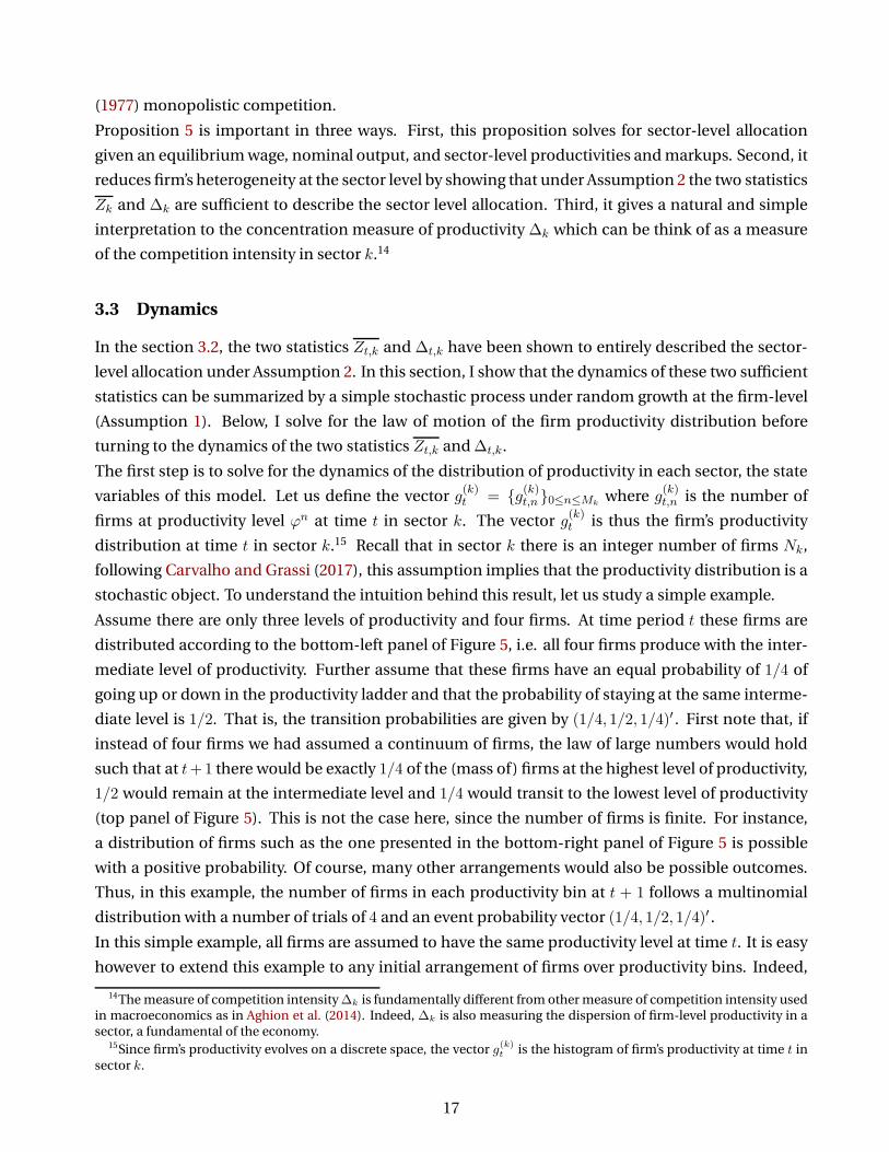
stochastic object. To understand the intuition behind this result, let us study a simple example.

Assume there are only three levels of productivity and four firms. At time period t these firms are

distributed according to the bottom-left panel of Figure 5, i.e. all four firms produce with the inter-

mediate level of productivity. Further assume that these firms have an equal probability of 1/4 of

going up or down in the productivity ladder and that the probability of staying at the same interme-

diate level is 1/2. That is, the transition probabilities are given by (1/4, 1/2, 1/4)′ . First note that, if

instead of four firms we had assumed a continuum of firms, the law of large numbers would hold

such that at t+1 there would be exactly 1/4 of the (mass of) firms at the highest level of productivity,

1/2 would remain at the intermediate level and 1/4 would transit to the lowest level of productivity

(top panel of Figure 5). This is not the case here, since the number of firms is finite. For instance,

a distribution of firms such as the one presented in the bottom-right panel of Figure 5 is possible

with a positive probability. Of course, many other arrangements would also be possible outcomes.

Thus, in this example, the number of firms in each productivity bin at t + 1 follows a multinomial

distribution with a number of trials of 4 and an event probability vector (1/4, 1/2, 1/4)′ .

In this simple example, all firms are assumed to have the same productivity level at time t. It is easy

however to extend this example to any initial arrangement of firms over productivity bins. Indeed,

14The measure of competition intensity ∆k is fundamentally different from other measure of competition intensity usedin macroeconomics as in Aghion et al. (2014). Indeed, ∆k is also measuring the dispersion of firm-level productivity in asector, a fundamental of the economy.

15Since firm’s productivity evolves on a discrete space, the vector g(k)t is the histogram of firm’s productivity at time t in

sector k.

17

Figure 5: An illustrative example of the productivity distribution dynamics

NOTE: Top panel, with a continuum of firms the transition is deterministic. Bottom Panel, with a finite number of firms

the transition is stochastic.

for any initial number of firms at a given productivity level, the distribution of these firms across

productivity levels next period follows a multinomial. Therefore, the total number of firms in each

productivity level next period, is simply a sum of multinomials, i.e. the result of transitions from

all initial productivity bins. The following proposition generalizes this example to determine the

dynamics of the distribution of firms’ productivity for any firm-level productivity process.

Proposition 6 (Sector k’s Productivity Distribution Dynamics) The Sector k’s Productivity Distribu-

tion satisfies the following law of motion

g(k)t+1 = (P(k))′g

(k)t + ǫ

(k)t (4)

where P(k) is the matrix of transition probabilities of the firm-level productivity process in sector k and

where ǫ(k)t =

ǫ(k)t,n

0≤n≤Mk

is a mean zero random vector.

Furthermore, under Assumption 1, the stationary distribution (when ∀t, ǫ(k)t = 0) is Pareto and equal

to g(k)n = NkKk(ϕ

nk )

−δk where Kk is a normalization constant and δk = log ak

ck/logϕk is the tail index.

Proof See Online Appendix F.2.

The above proposition described the law of motion of a sector’s productivity distribution and cap-

ture exactly the intuition of the example in Figure 5. The first term of the right hand side of the law

of motion 4 is the average behavior of the sector’s productivity distribution. If there were an infinite

number of firms, this average behavior would be exactly the next period sector’s productivity distri-

bution. Note that this term is solely a function of the current period productivity distribution g(k)t

18

and the transition probabilities of the firm level productivity process P(k). Because there are a finite

and integer number of firms in each sector, there is a extra term, ǫ(k)t . This second term is the devia-

tion of the actual realization of g(k)t+1 and its average behavior. As described in the example above, for

a given period t, this random vector is a sum of demeaned multinomial random vectors.

A direct implication of this proposition is that sectors’ productivity distribution, the state variables of

this framework, are stochastic vectors. It follows that every sectors’ variables are themselves stochas-

tic and fluctuate. Finally, these sectors’ productivity distribution hover around their stationary value

which are, under Assumption 1, Pareto distributed with a tail index determined by the probabilities

ak and ck.16

Note that no aggregate or sector-level shocks are assumed, instead this sector (and aggregate) level

fluctuations arise from independent firm-level shocks. The quantitative importance of such fluc-

tuations is not formally discussed here and is addressed numerically below where the above model

is calibrated to the US economy. However, the diversification among these firm-level independent

shocks is weak as soon as the stationary Pareto distributions is fat-tail. As it is shown by Gabaix

(2011), when it exists a small number of very productive firms, it is very unlikely that shocks to these

firms cancel out and therefore they translate into quantitatively important fluctuations.17

After the characterization of the dynamics of the sector’s productivity distribution (Proposition 6),

the second step is to describe the law of motion of the two statistics Zt,k and ∆t,k that are sufficient

under Assumption 2. Proposition 7 below shows that under random growth (Assumption 1) the law

of motion of these two statistics can be described by a simple process.

Proposition 7 (Dynamics of Zt,k and ∆t,k) Under Assumption 1, the two statistics Zt,k and ∆t,k of the

sector k’s productivity distribution satisfy the following dynamics:

Zt+1,k = ρ(Z)k Zt,k + o

(Z)t,k +

√(Z)k ∆t,k +O

(Z)t,k Zt,k ε

(Z)t+1,k

(Zt+1,k

Zt,k

)2

∆t+1,k = ρ(∆)k ∆t,k + o

(∆)t,k +

√(∆)k χt,k +O

(∆)t,k ∆t,k ε

(∆)t+1,k

where ε(Z)t+1,k and ε

(∆)t+1,k are random variables following a N (0, 1) with a non-zero covariance and

where χt,k, o(Z)t,k , o

(∆)t,k , O

(Z)t,k and O

(∆)t,k are predetermined at time t, while, ρ

(Z)k , ρ

(∆)k ,

(Z)k and

(∆)k are

constant.

Proof See Online Appendix F.3.

Proposition 7 is similar to Theorem 2 of Carvalho and Grassi (2017). It shows that the dynamics of

the two moments of the sector k’s productivity distribution are persistent. The intuition is that since

the firm-level productivity is itself persistent, this persistence is aggregated at the sector level. The

higher is the firm-level persistence, higher is the sector-level persistence as shown in Carvalho and

16The concept of a stationary distribution is the same as in Hopenhayn (1992) and Hopenhayn and Prescott (1992).17In a one sector model with perfect competition and entry/exit à la Hopenhayn (1992), Carvalho and Grassi (2017) study

the behavior for an increasingly large number of firms of the volatility arising from idiosyncratic independent shocks onfirms.

19

Grassi (2017).18

Moreover, the (conditional) variance of the sum of the productivity of sector k’s firms, Zt,k, is time

varying and is determined by the Hearfindahl index of firms’ productivity ∆t,k. Here as in Gabaix

(2011) and Carvalho and Grassi (2017), any volatility at the sector level is due to idiosyncratic shocks

at the firm level. When a sector is concentrated, shocks to firms with a large productivity do not

wash out at the aggregate level. A higher concentration implies a higher importance of these firms

and thus more volatility due to idiosyncratic shocks.

4 Structural Firms

In this section, I show that the structural importance of a firm is determined by the firm’s size, the

firm’s sector industrial organization and its role in the input-output network. The structural impor-

tance of a firm is defined here as the elasticity of aggregate output with respect to the productivity of

one firm in one sector.

In order to compute this elasticity, the first step is to solve for the aggregate output and the equilib-

rium wage. I assume that the household supplies inelastically one unit of labor and I normalized the

price of the composite consumption good to one. The following proposition describes the equilib-

rium allocation given sector-level markups and productivities.

Proposition 8 (Equilibrium Allocation) For given sector-level markups µk and productivities Zk, the

wage is

logw = −β′(I − Ω)−1log µkZ

−γk

k

k= −

N∑

k=1

βk log µkZ−γk

k (5)

where β is the (N × 1)-vector of the household expenditure share βkk andβk′k= β′(I − Ω)−1 are

the sectors’ centrality. The share of aggregate profit in nominal output is

Pro

PCC= β′(I − Ω)−1

1− µ−1

k

k=

N∑

k=1

βk

(1− µk

−1)

(6)

where Ω = diag(µ−1k

k

)Ω with diag (xkk) is the diagonal matrix whose non-zero elements are

the xk and where µk is such that1− µk

−1k= (I − Ω)−1

1− µ−1

l

l. Finally, aggregate output is

log Y = logw − log

(1− Pro

PCC

)(7)

Proof See Appendix A.4.

The equilibrium wage of Equation 5 comes from sectors’ price (Equations 2) and the normalization

PC = 1. Note that the log of wage can be rewritten as a weighted sum of sector level markups and

18For n ∈ N∗, the sequences vk,n = akϕ

−n(εk−1)γkk + bk + ckϕ

n(εk−1)γkk and wk,n = akϕ

−2n(εk−1)γkk + bk + ckϕ

2n(εk−1)γkk −

(ρ(n)k )2 are respectively the mean and variance of the growth rate of firm i in sector k productivity measure Z(k, i)n(εk−1)γk .

We have that, ρ(Z)k = vk,1, ρ

(∆)k = vk,2,

(Z)k = wk,1 and

(∆)k = wk,2.

20

productivities where the weights areβk′k= β′(I−Ω)−1 = β′(I+Ω+Ω2+ . . .) the sectors’ centrality.

The centrality measures the direct and indirect importance of a sector in the household consump-

tion bundle. A sector’s good contributes to the consumption bundle by the direct consumption of

this good by the household. This is governed by the shares β. This good is also used as input by other

sectors that are themselves consumed by the household. This first-degree indirect contribution to

the household consumption bundle is captured by the therm β′Ω. Furthermore, this good is also

used as inputs for other goods that are themselves inputs of other goods that are consumed by the

household. This second-degree indirect importance is captured by the term β′Ω2. Higher degree

linkages are captured in the same way. The centrality is then the infinite sum of these terms which

is then equal to the product of the share β and the Leontieff inverse (I − Ω)−1. The centralities βk

take into account the direct and indirect consumption of a sector’s good through the input-output

network.

The aggregate profit share is a function of sectoral markups and the input-output network. To under-

stand the intuition behind Equation 6, let us compute the profit share of one dollar spend on sector k

in the simple input-output network of Figure 4. The sector-level markup determines the profit share:

a share 1−µ−1k of this dollar is directly rebated to the household as profit. The remaining, µ−1

k , is used

to pay for inputs among which the sector l’s good. Therefore, sector l receives µ−1k ωkl of income of

the dollar spend on sector k, from which a share 1−µ−1l is rebated to the household. The total profit

rebated to the household of this dollar spend on sector k is then equal to 1− µ−1k + µ−1

k ωkl

(1− µ−1

l

).

Equation 6 is a generalization of this intuition to any input-output structure. The element µ−1k ωk,l of

the matrix Ω is the income share that goes from sector k to sector l. The Leontieff inverse of this ma-

trix, (I − Ω)−1, gives the direct and indirect income share that goes from one sector to another while

the vector1− µk

−1k

gives the income share of each sector that is directly rebated to the house-

hold. The aggregate profit share can also be rewritten as a weighted sum of the expenditure share βk

where the weights 1−µk−1 are the direct and indirect profit share of each sector k. Note also that µk−1

is the direct and indirect labor share of each sector and it is such that µkk = (I − Ω)−1γkµ−1k k.19

The aggregate output equation comes from the household budget constraint and the inelastic labor

supply. Note that this equation will be different for different utility function. Appendix D derives

the case of elastic labor supply for both separable and Greenwood–Hercowitz–Huffman (GHH) pref-

erences. Under Assumption 2, the results in Propositions 8 and 5 describe entirely the equilibrium

allocation as a function of the two sufficient statistics Zk and ∆k. The first part of Proposition 5

and Proposition 8 solve for the equilibrium allocation as a function of sector-level markups and pro-

ductivities, while the second part of Proposition 5 gives the sectors’ markup and productivity as a

function of these two sufficient statistics.

Let us decompose the effect of an increase in productivity of one firm in one sector on aggregate

output into the “downstream” and “upstream” part of aggregate output. The “downstream” part of

aggregate output is defined as the first term of the right hand side of Equation 7: log Y d = log wP L =

logw. This is minus the (log) real labor income, since total labor and the composite good price are

19This can be shown using the definition of µk−1 and the fact that Ω1k = diag(µ−1

k k)Ω1k = µ−1k (1− γk)k.

21

normalized to one. The “upstream” part is defined as log Y u = − log(1− Pro

PCC

)= − log

(wLPCC

)this is

the (log of) the labor share. Therefore, this decomposition of aggregate output is just a decomposi-

tion in term of real labor income and the labor share. The terminology “downstream” comes from

the fact that any change in a sector’s price impacts the downstream sectors and is reflected in the

wage. The “upstream” terms comes from the fact any change in markups and thus cost share im-

pact the income share received by the upstream sectors and is ultimately reflected in the aggregate

profit/labor share.20 The elasticity of aggregate output to the productivity Z(k, i) of firm i in sector k

is then the sum of the effect on the “downstream” and “upstream” part of aggregate output:

∂ log Y

∂ logZ(k, i)︸ ︷︷ ︸change in GDP

=∂ log Y d

∂ logZ(k, i)︸ ︷︷ ︸change in labor income

+∂ log Y u

∂ logZ(k, i)︸ ︷︷ ︸-change in labor share

First, let us look at the effect of a change in productivity of one firm in one sector on the labor in-

come. The change of the “downstream” part of aggregate output captures any change on the real

wage. These changes are themselves due to changes on sectoral prices. Changes in sectoral prices

propagate to downstream sector. To understand this, let us once again look at the simple input-

output of Figure 4. Recall that in this simple case the sector k’s price is

log Pk = log µk + log

(w

Zk

)γk

+ ωk,l logPl with log Pl = log µl + log

(w

Zl

)

Following a change of the productivity of one firm in sector l, the two statisticsZl and ∆l are affected

as described in Section 3.1. These changes affect the markup µl and the productivity Zl in sector l

(Proposition 5) which in turn affect the price in sector l. Any change in sector l’s price impacts the

marginal cost of the downstream sector k and therefore the price of sector k. Any shocks on firms

in a sector propagate to downstream sectors through the price. This is ultimately affecting price

of all downstream sectors and thus the real wage i.e the “downstream” part of aggregate output.

The strength of this effect depends on (i) the pass-through in sector l, i.e on how much the sector

l’s price changes after the increase in productivity of one of its firms, and, on (ii) the input-output

linkage between sector l and sector k. The market structure of the sector and the identity of the firms

whose productivity increases determine the strength of the pass-through. Proposition 9 computes

the elasticity of the “downstream” part of aggregate output with respect to the productivity of one

firm in one sector for any input-output network.

Proposition 9 (Elasticity “downstream”) Assume 2, the elasticity of the “downstream” part of aggre-

gate output with respect to the productivity of firm i in sector k is

∂ log Y d

∂ logZ(k, i)=

βkεk − 1

(1 +

2ek∆k

(∆k −

Z(k, i)(εk−1)γk

Zk

))∂ logZk

∂ logZ(k, i)

where ek = d log fkd log∆k

andβk′k= β′(I − Ω)−1 is the vector of sectors’ centrality.

20See Section 5 for a study of propagation of firm-level shocks across sectors.

22

Proof See Appendix A.5.

The elasticity of the “downstream” part of aggregate output with respect to the productivity of firm

i in sector k is the product of three terms. The first term is the sector’s centrality βk. As discussed

earlier, the centrality measures the direct and indirect importance of a sector in the household con-

sumption bundle. The second term captures the effect of oligopolistic competition, under monopo-

listic competition this term would be equal to one. Whenever the firm i in sector k is “large”, i.e whenZ(k,i)(εk−1)γk

Zk> ∆k, this second term is smaller than one. Because, when the productivity of a large

firm increases some of the productivity gains translates in an increase of markup rather than a fall

in price. Indeed, this firm already have a lot of market power and does not need to cut its price and

increase its production by as much as under monopolistic competition: the pass-through is incom-

plete. At the sector level the price falls by less than under monopolistic competition and the effect on

the “downstream” part of aggregate output is smaller. Conversely, if the productivity of a “small” firm

increases, i.e whenZ(k,i)(εk−1)γk

Zk< ∆k, the second term is larger than one. When the productivity of

this firm increases, it decreases its price and increases its markup but also cuts the markups of larger

firms. At the sector level, the price fall by more than under monopolistic competition and the effect

on the equilibrium wage and the “downstream” part of aggregate output is stronger. The last term

is the effect of the firm’s increase in productivity on the first moment of the sector k productivity

distribution. The more productive is the firm affected, the larger is this term.

The elasticity of the “downstream” part of aggregate output reflects the effect of the change in price

on the real wage following an increase in Z(k, i). It is easy to see this by rewriting the change in the

“downstream” part of aggregate output as:21

∂ log Y d

∂ logZ(k, i)= βk

(1

εk − 1

∂ logZk

∂ logZ(k, i)−

εkεk−1 − 1

µk − 1

∂ log µk∂ logZ(k, i)

)(8)

The centrality βk is the importance of the firm’s sector good in the determination of the wage. The

first term in the bracket is equal to the change in the monopolistic competition (complete pass-

through) sector k’s price following the increase in the productivity of firm i. The second term in

the bracket is the change in sector’s markup due to the change in firm i’s productivity. This last

term would be equal to zero under perfect competition. As described earlier, this term can be either

negative or positive depending on the identity of the firm subject to the shock.

The structural importance of a firm for the “downstream” part of aggregate output is a function of

the input-output network through the sector’s centrality, the sector’s market structure index by the

∆k, and, the firm size through the term ∂ logZk

∂ logZ(k,i) . The market structure and the firm size govern

the change in sector’s price following a change in the firm’s productivity, while the input-output

linkages determine the intensity of the effect of this change in sector’s price on other sectors and on

the equilibrium wage.

Let us now study the effect of a change in productivity of one firm in one sector on the labor share.

21Note that using the expression of the markup under Assumption 2 (Proposition 5) and the elasticity of ∆k to Z(k, i) in

Section 3.1, it is easy to show that the elasticity of the markup is ∂ log µk∂ logZ(k,i)

= −(µk − 1) 2ek∆k

(∆k − Z(k,i)(εk−1)γk

Zk

).

23

The change of the “upstream” part of aggregate output captures any change on the aggregate labor

and profit income share. These changes are themselves due to changes on sectoral profit share.

Changes in sectoral profit share affect the income received by the upstream sectors. To understand

this, let us look at the profit share of a dollar spend on sector k’s good in the simple input-output

structure of Figure 4. In this simple example, the share of profit of one dollar spend on sector k’s

good is 1− µk−1 + µk

−1ωkl

(1− µl

−1). Following a shock on the productivity of firm i in sector k, the

statistic ∆k changes, let assume it increases. This increase in ∆k increases µk, the markup in sector

k (Proposition 5). As a consequence less income is used to pay for inputs among which sector l’s

good. The total share of profit/labor is affected because (i) the sector k rebates more profit to the

household and (ii) the upstream sector l receives less income and therefore rebates less profit to the

household. Proposition 10 generalizes the above intuition to any input-output structure.

Proposition 10 (Elasticity “upstream”) Assume 2, the elasticity of the “upstream” part of aggregate

output with respect to the productivity of firm i in sector k is

∂ log Y u

∂ logZ(k, i)= −P

CC

wL

PkYkPCC

(µk − 1)

µk

2ek∆k

(∆k −

Z(k, i)(εk−1)γk

Zk

)∂ logZk

∂ logZ(k, i)

where ek = d log fkd log∆k

is the elasticity of fk, and where µk is such that1− µk

−1k= (I − Ω)−1

1− µ−1

l

l

with

Ω = diag(µ−1k

k

)Ω.

Proof See Appendix A.5.

The elasticity of the “upstream” part of aggregate output is the product of several terms. The first im-

portant term, µk−1, is the cost share of sector k’s income that is rebated as labor income to the house-

hold directly and indirectly through other sectors. The second important term is proportional to the

change in sector’s cost/profit share, 2ek∆k

(∆k − Z(k,i)(εk−1)γk

Zk

)∂ logZk

∂ logZ(k,i) . Under monopolistic competi-

tion, i.e when ∆k → 0, this term is zero. Under oligopolistic competition, this term can be either

positive or negative. Whenever the firm i in sector k is “large”, i.e when Z(k,i)(εk−1)γk

Zk> ∆k, this term is

negative and ∂ log Y u

∂ logZ(k,i) becomes positive. This is very intuitive, when the productivity of a large firm

increases this firms reduces its price but also uses its market power to raise its markup. At the sector

level the profit share is higher which translates to a higher (resp. lower) aggregate profit share (resp.

labor share) and a higher “upstream” part of aggregate output. Conversely, when the productivity of

a “small” firm increases, i.e whenZ(k,i)(εk−1)γk

Zk< ∆k, this term is positive and the elasticity of the “up-

stream” part of aggregate output is negative. This is because when the productivity of a “small” firm

increases, this firm decreases its price and increases its markup but also cuts the markup of larger

firms. At the sector level, the markup is reduced which translates in smaller (resp. larger) profit

share (resp. labor share). The aggregate profit share (resp. labor share) is therefore reduce and so is

the “upstream” part of aggregate output. The elasticity of the “upstream” part of aggregate output

reflects the effect of the change in cost share on the aggregate labor share following an increase in

24

Z(k, i). To see this, one can rewrite this elasticity as follow:

∂ log Y u

∂ logZ(k, i)= − PkYkµk

−1

wL

∂ log(µ−1k )

∂ logZ(k, i)

This expression shows that the effect on the aggregate labor income, the upstream part of aggregate

output, is determined by sector k’s direct and indirect labor share and the elasticity of sector k’s cost

share. Sector k’s direct and indirect labor share is measured as a share of the total labor income by

the sales of sector k, PkYk, of which a share µk−1 is rebated directly and indirectly as labor income.

Sector k’s cost share is µ−1k , because of oligopolistic competition this share is affected by changes in

productivity of firms in sector k.

Both the market structure and the input-output network impact the propagation of firm level shocks

on the “upstream” part of aggregate output. The markup centrality µk is jointly determines by the

input-output network and the competition intensity through the matrix Ω whose elements gives the

income share that flows between two sectors.

As a conclusion, the structural importance of a firm is determined by the firm size, the market struc-

ture and the input-output network. The size determines the influence of a firm on sector’s price

and profit share. The input-output network determines the importance of a sector in the consump-

tion bundle and the aggregate profit/labor share. The sector’s market structure interacts with both

the firm size and the input-output network in shaping the structural importance of a firm. Indeed,

with the firm size it governs the strength of the change in sector’s price and profit share following a

shock on one firm, and, with the input-output network it governs the importance of a sector for the

aggregate profit/labor share.

The decomposition between the “downstream” and “upstream” part of aggregate output is valid be-

cause I assume an inelastic labor supply. In this case, any change in profit/labor share does not

feed back to the wage by affecting the labor supply, while the effect of a wage increase on aggregate

output is not magnified by an endogenous increase in labor supply. Relaxing the inelastic labor sup-

ply assumption won’t affect the results but it affects the interpretation of the terms “downstream”

and “upstream”. As shown in Appendix D, with separable or GHH preferences, the output is still

a function of the wage and the profit/labor share. They are themselves only a function of sectoral

productivities and markups (Proposition 8) and therefore, under Assumption 2, a function of the

statistics Zk and ∆k (Proposition 5).

5 Propagation

In this section, I show how a shock on one firm in one sector propagates to other sectors through

the input-output network. The propagation to downstream sectors is due to change in price whose

magnitude is governed by the competition intensity. The new propagation mechanism to upstream

sectors is entirely due to the endogenous change in cost/profit share. To study the propagation of

firm-level productivity shocks in the economy, I derive the elasticity of sector-level price (Proposi-

25

tion 11) and sales share (Proposition 12) with respect to the productivity of one firm in one sector.

These results together with the elasticity of aggregate output derived in the previous section (Propo-

sitions 9 and 10) allow to derive the effect of an increase in productivity of one firm in a sector on

sector-level output.

The effect of a change in productivity of one firm on other sectors’ price is summarized in Proposi-

tion 11 by the elasticity of sector k’s price with respect to the productivity of firm j in sector l.

Proposition 11 (“Downstream” Propagation) Assume 2, the elasticity of the sector k’s price with re-

spect to the productivity of firm j in sector l is

∂ log Pk

∂ logZ(l, j)=

∂ logw

∂ logZ(l, j)−

ψdk,l

εl − 1

(1 +

2el∆l

(∆l −

Z(l, j)(εl−1)γl

Zl

))∂ logZl

∂ logZ(l, j)

where ek = d log fkd log∆k

is the elasticity of fk, and ψdk,l is the element (k, l) of the matrix ψd = (I − Ω)−1.

Proof See Appendix A.6.

The change in sector k’s price reflects the change in cost. It is the sum of the change in labor and

intermediate goods cost. Following a change in productivity of firm j in sector l, the wage changes

as it is described in the previous section and in Proposition 9. This is the structural importance of

the firm j in sector l on the wage. This change in wage affects the cost of labor and thus sector k’s

price.22

The change in intermediate goods price is captured by the second term which is the product of (i)

the direct and indirect exposure of sector k’s production to sector l’s good, (ii) the effect of oligopolis-

tic competition in sector l, and, (iii) the effect of the change in productivity of firm j on sector l’s.

The degree of direct and indirect exposure of sector k’s production to sector l’s good is measured by

ψdk,l the element k, l of the matrix (I −Ω)−1. In the simple input-output structure of Figure 4 this pa-

rameter is exactly equal to ωk,l. For a more general input-output structure, the number ψdk,l captures

the dependence of sector k’s production on sector l’s good directly and through other sectors. For

example, let us assume that the input-output network is as in Figure 6 i.e. sector k’s is using sector l

and sectorm’s goods to produce, and, sectorm is also using sector l’s good to produce. In this simple

case, the direct and indirect exposure of sector k’s production to sector l’s good, ψdk,l, is taking into

account the direct consumption of sector l’s good by sector k plus the indirect consumption of sector

l’s good through sectors m, as the latter is also using l to produce its good: ψdk,l = ωk,l + ωk,mωm,l.

The effect of oligopolistic competition is similar as the one described in the previous section, it mea-

sures the pass-through of the increase in productivity of firm j on sector l’s price. Under monop-

olistic competition the term 1 + 2el∆l

(∆l − Z(l,j)(εl−1)γl

Zl

)would be equal to one. Here, depending on

the identity of the firm j, the response of sector l is larger or smaller than under monopolistic com-

petition. If the productivity of a large firm increases, i.e Z(l,j)(εl−1)γl

Zl> ∆l, some of the increase in

productivity translates in an increase in markup at the sector level and therefore the sector l’s price

22Note that this change in wage affects all the sector in the economy and therefore it also indirectly affects sector kthrough its intermediate input consumption. This is the reason why there is no parameter γk, the labor share, in front ofthe term ∂ logw

∂ logZ(l,j).

26

Figure 6: An Example of Input-Output Structure

mk l

ωk,m ωm,l

ωk,l

NOTE: In this simple input-output structure, firms in sector k are using labor, sector l and sector m’s goods to produce their

variety, firm in sector m are using labor and sector l’s good, while firms in sector l are using only labor.

fall by less than under monopolistic competition. Conversely, if the increase in productivity affects

a small firm, i.eZ(l,j)(εl−1)γl

Zl< ∆l, this firms is cutting the markup of its larger competitors and thus

reduces the markup at the sector level. In this case, sector l’s price falls by more than under mo-

nopolistic competition. One can see this more clearly by rewriting the elasticity of sector k’s price

as:∂ log Pk

∂ logZ(l, j)=

∂ logw

∂ logZ(l, j)− ψd

k,l

(1

εl − 1

∂ logZl

∂ logZ(l, j)−

εlεl−1 − 1

µl − 1

∂ log µl∂ logZ(l, j)

)

The effect on sector k’s price is stronger or smaller depending on the sign of the elasticity of sector l’s

markup with respect to Z(l, j). As it is described above the sign of this elasticity is a function of the

identity of firm j.

Without an input-output network, the term ψdk,l would be replace by one for k = l and by zero other-

wise i.e. a shock to one firm in a sector affects others sectors only through the effect on wage. With

an input-output network but without oligopolistic competition, the sector l’s markup would be con-

stant i.e. ∂ log µl

∂ logZ(l,j) = 0. In that case, only the size of the firm would matter through ∂ logZl

∂ logZ(l,j) and the

market structure in the sector would be irrelevant.

Let us now look at the effect of a change in productivity of one firm on other sectors’ sales share,

this is summarized in Proposition 12 by the elasticity of sector k’s sales share with respect to the

productivity of firm j in sector l.

Proposition 12 (“Upstream” Propagation) Assume 2, the elasticity of the sector k’s sales share with

respect to the productivity of firm i in sector l is

∂ log(PkYk

PCC

)

∂ logZ(l, j)= (ψs

l,k − Il,k)PlYlPkYk

(µl − 1)2el∆l

(∆l −

Z(l, j)(εl−1)γl

Zl

)∂ logZl

∂ logZ(l, j)

where ek = d log fkd log∆k

is the elasticity of fk, Il,k is equal to one if k = l and zero otherwise ,and, ψsl,k is the

element (l, k) of the matrix ψs = (I − Ω)−1.

Proof See Appendix A.7.

The change in sector k’s sales share reflects the change in demand from sector l. The demand from

sector l is determined by the total cost share of sector l and the exposure of the sector k to sector

27

l demand. Any change in the cost share is a change of the opposite sign of the profit share. For

example, after an increase of the profit share, more income is rebated to the household as profit

and less income is used to pay for inputs. Following an increase in productivity of firm j in sector

l the profit share changes, and depending on the identity of firm j, it can increase or decrease. If j

is large, i.e ∆l <Z(l,j)(εl−1)γl

Zl, the gain in productivity translates in an increase in markup and thus

of the profit share. Conversely, if j is small, i.e ∆l >Z(l,j)(εl−1)γl

Zl, the increase in firm j’s productivity

cuts the markup of its larger competitors in sector l and the profit share at the sector level increases.

The sector l’s cost share is µ−1l and it is easy to rewrite the elasticity of the sector k’s sales share as a

function of the change in cost share:

∂ log(PkYk

PCC

)

∂ logZ(l, j)= (ψs

l,k − Il,k)PlYlPkYk

∂ log µ−1l

∂ logZ(l, j)(9)

This elasticity is the product of three terms. The last two terms represent the change in total cost in

sector l as a share of sector k’s sales share. It is the product of sector l’s income and the change in

sector l’s cost share following an increase in productivity of firm j in sector l. The first term repre-

sents the exposure of sector k to the direct and indirect demand of sector l. The number ψsl,k, i.e the

element (l, k) of the matrix (I − Ω)−1, is the share of sector l’s income that goes to sector k directly or

indirectly through other sectors. To understand this, let us assume that the input-output network is

the simple one of Figure 6. In this case, the number ψsk,l takes into account the direct income share

used by sector k to pay for the input of sector l’s good. It also takes into account the indirect income

share of sector k that goes to sector l through sector m since the latter is also using sector l’s good to

produce. In the simple case of Figure 6 we have ψsk,l = µ−1

k ωk,l + µ−1k ωk,mµ

−1m ωm,l.

Note that the sector k’s sales share would be kept constant if there were no input-output network. In

that case, ψs = I and the first term of Equation 9 would be zero. Without an input-output network

all the demand comes from the household who are spending a constant share of their income on

each goods thanks to the Cobb-Douglas preferences. Even if the increase in productivity of firm j

in sector l is affecting aggregate income (see Section 4) it is not affecting one sector more than the

others. Note also that the sector k’s sales share would be constant if monopolistic competition were

assumed. In that case, the sector l’s cost share would be fixed and the last term of Equation 9 would

be zero. Without oligopolistic competition the change in productivity of firm j in sector l is not

affecting the sector-level markup and the repartition of income between inputs and profit is fixed

by the value of the parameter εk. The propagation mechanism of Proposition 12 requires both an

input-output network and an endogenous market structure to operate.

Proposition 11 relates to the “downstream” propagation since sector l’s shock is affecting sector k

strongly for higher value of ψdk,l. This is the element (k, l) of the matrix (I − Ω)−1 which measure

the direct and indirect cost share of sector l’s good in sector k production: the good is going from

sector l to sector k i.e. sector k is downstream to sector l. Proposition 12 relates to the “upstream”

propagation since shock to sector l is affecting sector k strongly for higher value of ψsl,k. This is the

element (l, k) of the matrix (I − Ω)−1 which measure the direct and indirect income share of sector

28

k’s good in sector l production: the good is going from sector k to sector l i.e sector k is upstream to

sector l. Note that here this notion of “downstream” and “upstream” are a generalization of the usual

definition to take into account the indirect linkages between sectors.

6 Quantitative Results

In this economy all the aggregate uncertainty comes from the firm-level productivity stochastic pro-

cess Zt(k, i). Since there is a finite number of firms in a sector, firm-level fluctuations translate into

sector-level fluctuations. However, these firms play an oligopolistic competition game and take into

account the impact of their decision on their sector. This results in incomplete pass-through of

shocks to price and fluctuations in profit share. When the firm-level productivity process is assumed

to follow random growth (Assumption 1) the two statistics Zt,k and ∆t,k are stochastic and follow

AR(1)-type processes (Proposition 7). While under Assumption 2 and under oligopolistic compe-

tition, fluctuations in these statistics create fluctuations in sector-level markups and productivities

according to Proposition 5. The origin of these sector-level fluctuations is “granular” (Gabaix, 2011)

and they are due to the presence of large firms in a given sector. Sectors are linked through a “small

world” input-output network (Figure 1) where there are a handful of hub-like sectors. Similar to

Acemoglu et al. (2012) and Carvalho (2010), sector-level fluctuations do not average out and create

sizable fluctuations in output as computed in Proposition 8.

In this section, I evaluate the quantitative importance of firm-level productivity shocks and

oligopolistic competition in shaping the business cycle. To this end, I first calibrate the above frame-

work to the US economy. I then simulate a path of firm-level productivity for each firms and I solve

for the equilibrium allocation at each period. I then compute business cycle statics and I decom-

pose aggregate volatility of output into fluctuations in labor income and labor share i.e. into the

“downstream” and “upstream” part of aggregate output.

6.1 Calibration and Numerical Strategy

To calibrate this economy the first step is to choose preferences and deep parameters of the model.

Consistently with the analysis in Section 4, I assume that labor supply is inelastic. Such assump-

tion allows to perform the decomposition of aggregate output between its “downstream” and “up-

stream” part.23 Appendix D shows how the results are affected by relaxing the inelastic labor supply

assumption. The second important assumption is the choice of the parameter εk, here I choose this

parameter to be equal to 5 in every sectors: ∀k, εk = 5. Even if this is a strong assumption, this value

seems reasonable as this number has been estimated in the international trade literature to be be-

tween 3 and 9 (see Imbs and Mejean (2015) for example). Note that the estimates in the international

trade literature are not necessary consistent with the above model as they are usually not assuming

23This assumption is also standard in the literature on the micro-origin of aggregate fluctuations and allow for compar-ison with Acemoglu et al. (2012), Baqaee (2016) or Baqaee and Farhi (2017a). Carvalho and Grassi (2017) assume elasticlabor supply and their results should be compare with result in Appendix D.

29

Table 2: Baseline Calibration

Parameters Value Description Target/Source

εk 5 substitution across firms Monop Markup 1.25

N 389 # of sectors BEA

Nk 578 median # firms in a sector Census data∑kNk 5 576 852 total # of firms Census data

∆k 0.037 median Pdty Herfindahl sales HHI of the Census

βk 0.027 median HH consumption share (%) BEA

γk 55.90 median labor share (%) BEA

Ω 2.19 I-O network density (when links> 1%, %) BEA

ak, ck 0.34,0.30 median Firm-level pdty process σk = 0.1 and ∆k

NOTE: The first column gives the notation of the parameter in the model. The third column gives the description of the

value in the second column. The fourth column is the data source or the calibration target associated.

oligopolistic competition. An elasticity of 5 across varieties within a sector implied a sectoral markup

for monopolistic competition of 1.25. Finally, the sector competition is assumed to be differentiated

Bertrand.

The second step consists to use concentration and input-output data to discipline the sector-level

parameters. For this calibration, a sector is an industry as defined by the Bureau of Economic Analy-

sis (BEA) in their detailed input-output classification. There are 389 sectors and the level of disagre-

gation is comparable for most sectors to the 5 digits NAICS classification. This is the most disaggre-

gated level available with sectoral input-output linkages information. The U.S. Census Bureau gives

information on sector-level concentration. I use the 2007 vintage of these data and especially the

Herfindahl-Hirchman-Index (HHI) of sales share among the top 50 firms, namely HHIk.24 Under

Assumption 2, it is easy to show that ∆k = f−1k

((1− ε−1

k

)HHIk + 1

). I am using this relationship

and the value of εk to back out the concentration measure of productivity at the sector level ∆k. With

these values in hand, I calibrate the Markov chain of the productivity process P(k) to match a firm

level volatility of σk = 0.1 and the value of ∆k. The firm-level volatility is at the lower hand of esti-

mate in the firm dynamics literature (see Foster et al. (2008) or Castro et al. (2015) for example). Note,

however, that the literature’s estimates are not necessarily consistent with the oligopolistic competi-

tion assumption in the framework presented in this paper. The matrix Ω is calibrated using the latest

vintage of the detailed input-output data of the BEA for 2007. For a description of the data see the

data Appendix B. The model counterpart of the input-output table provided by the BEA is Ω whose

elements are the share of income that goes from one sector to the other. Using the concentration,

I compute the sector-level markup and I use the relation between Ω and Ω = diag(µ−1k k)Ω to re-

cover the actual Ω whose elements are the share of total cost that goes from one sector to the other.

As one can see in Figure 1 and as it has been shown in Acemoglu et al. (2012) or Carvalho (2014) this

input-output network is a “small world” network where a handful of sector are heavily connected to

the other sectors.

24These data are described in Appendix B.

30

Table 2 summarizes the parameters of the baseline calibration. In this calibration there are N = 389

sectors, the median number of firms in each sector is 578 while the total number of firms is equal

to almost 5.6 millions firms. The median value of ∆k across sector is 0.037 which implies a value of

the HHI of 0.063. Note that merger law starts to apply in the US for a value of the HHI over 0.18. The

value of the median markup is about 1.27. Under monopolistic competition this markup would be

1.25 for a value of εk = 5. In this calibration the median sector is relatively close to a sector under

monopolistic competition, it reflects the conservatism of the baseline calibration. Finally, the input-

output network has a density of 2.19% and is very sparse i.e. 2.19% of all the possible N2 = 151321

links have a value higher than 1%.

6.2 Aggregate Volatility and Variance Decomposition

For each of the 5.6 millions firms, I simulate a path of productivity of 4000 periods.25 To do so I use

the Proposition 6 and simulate the law of motion of the productivity distribution for each sector.

As in Carvalho and Grassi (2017), I follow the number of firms in each productivity bins rather than

following the path of each firms. It reduces considerably the computation cost of simulations. Note

that even if Assumption 2 is key for this calibration strategy by allowing the mapping between the

HHI and the productivity concentration measure ∆k, this assumption is not necessary to solve for

the equilibrium allocation given the firm productivity distribution at each period. Therefore, for

each period t, I solve for the full problem at the firm level from which I recover sector-level markups

and productivities that I aggregate in Yt using the Proposition 8.26 For this 4000 periods time series,

I compute aggregate volatility measured by the standard deviation of the percentage deviation of

aggregate output Yt. In Table 3, I decompose the variance of aggregate output between the contribu-

tion of the labor income and the labor share i.e the “downstream” and “upstream” part of aggregate

output as in Section 4:

Var[log Yt

]= Var

[log Y d

t

]

︸ ︷︷ ︸variance of labor income

+ Var[log Y u

t

]

︸ ︷︷ ︸variance of labor share

+ COV︸ ︷︷ ︸

covariance term

(10)

The first result is that the standard deviation of aggregate output Yt is 0.62%. The same number in the

Fernald (2014) data is 1.83%.27 So the aggregate volatility in this model is 0.62/1.83 = 33.88% of the

aggregate volatility observed in the data. Note that in this model this aggregate volatility is arising

purely from 5.6 millions independent firm-level shocks. The reason why this number is quantita-

tively non-negligible is that the central limit theorem and the “diversification argument” introduced

by Lucas (1977) fail to apply. The first reason why the central limit argument fails to apply is that the

diversification across firms within a sector is weak. Indeed within a sector, large firms represent a

25I simulate 5000 periods and drop the first 1000 periods.26Rather than solving the firm-level problem for each firms, I solve this problem for each productivity bins since all the

firms in a bins are perfectly homogeneous. More detailed can be found in the numerical Appendix C.27This number is the standard deviation of the percentage deviation of aggregate output from an HP trend as it is com-

puted in Carvalho and Grassi (2017).

31

Table 3: Aggregate Volatility

Total Downstream Upstream COV

sd [log Yt] 0.62 0.581 0.07

Var [log Yt] 100 89.03 1.33 9.64

NOTE: First row is the standard deviation of the percentage deviation of aggregate output Yt, of the “downstream” and

the “upstream” part of aggregate output as defined in Section 4. The second row is the variance decomposition of the

percentage deviation of aggregate output Yt in Equation 10 between the contribution of labor income and labor share,

i.e. the “downstream” and the “upstream” part of aggregate output. Numbers are reported in percentage points. These

statistics comes from a 4000 periods simulations.

disproportionate market share as it is observed in the Census Bureau concentration data. The “gran-

ular hypothesis” introduced by Gabaix (2011) is at play: shocks to these large firms do not average

out. Following a shock to one of these large firms it is unlikely that another shock of the opposite sign

hits another large firm and mitigate the first one. The second reason why the central limit argument

is not applying, is that the diversification across the 389 sectors is governed by the “small world”

input-output network where it exists a handful of highly connected hub-like sectors. As shown by

Acemoglu et al. (2012) and Carvalho (2010) diversification across sectors is weaker than without such

input-output network and translates into aggregate volatility.

The second results is that 89.03% of the aggregate variance is due to the labor income i.e. the “down-

stream” part of aggregate output while the labor share, the “upstream” part of aggregate output,

represents 1.33%, and, the covariance is about 9.64% of the aggregate variance. In an economy, with-

out oligopolistic competition all the aggregate volatility would be due to the downstream part of

aggregate output as the labor share, the “upstream” part would be constant. This illustrates the im-

portance of the role played by the propagation of changes in profit share and competition intensity

following firm-level shocks. Consistently with the Section 4’s results of Propositions 9 and 10, the

fact that the contribution of the “downstream” part of aggregate volatility is reduced compare to the

monopolistic competition case indicates that aggregate fluctuations are led by shocks on large firms

in their sectors. Following a shock on one of these large firms, the reduction in sector level price

that propagates to downstream sectors is smaller as some of the gain in productivity are captured by

an increase in markup. If instead the downstream propagation would have been higher than under

monopolistic competition, that would have meant that fluctuations would have been led by shocks

on medium size firms. Indeed, a positive shock on one of these firms translates into a higher fall

in sector’s price since some of this productivity gain is also reducing the sector’s markup and thus

strengthening the downstream propagation.

Let us further decompose the labor income i.e. the “downstream” part of aggregate output into the

contribution of the wage under monopolistic competition and the contribution of the change in

32

Table 4: Aggregate Variance Decomposition

“downstream” “upstream” COV

wage under monop. competition intensity COVwVar [log Yt] 89.03 1.33 9.64

Var [log Yt] 102.99 2.46 -16.42 1.33 9.64

Var[log YMonop

t

]100 0 0 0 0

NOTE: First row is the variance decomposition of the percentage deviation of aggregate output Yt between the its “down-

stream” and the “upstream” part. The second row include the decomposition of the “downstream” part of aggregate output

between Yd:Zkt and Y

d:∆kt . The third row is the decomposition under monopolistic competition.

competition intensity:

Var[log Y d

t

]= Var

[logwtL

]= Var

[logwmonop

t︸ ︷︷ ︸wage under monopolistic

]+ Var

[logwt − logwmonop

t︸ ︷︷ ︸competition intensity

]+ COVw

︸ ︷︷ ︸covariance term

Under Assumption 2, Equation 5 and Proposition 5 show that under monopolistic competition the

wage and the labor income,wmonopt , at time t is entirely determined byZt,k. Whereas the term logwt−

logwmonopt = −β′(I − Ω)−1log fk(∆t,k)

1

εk−1 k is entirely determined by the competition intensity

measured by the statistic ∆t,k. From the expression of the elasticity of the “downstream” part of

aggregate output in Equation 8 the interpretation of this decomposition is even clearer: the first

term is as if the sector-level markup were assumed to be fixed, while the second term is the change

in the profit share. Table 4 shows the decomposition the “downstream” part of aggregate output.

The first row of Table 4 reproduces the decomposition between “downstream” and “upstream” of

Table 3. In the second row the variance of aggregate output is further decomposed into the contri-

bution of the labor income under monopolistic competition and the contribution of the change in

competition intensity. The third row is the same decomposition for the case of monopolistic compe-

tition. Under monopolistic competition all the volatility of aggregate output is due to change in the

sum of productivity, while change in productivity concentration would have no effect. The volatil-

ity of aggregate output under monopolistic competition is 0.63 or 34.43% of the observed aggregate

volatility in the data. From an aggregate perspective, the aggregate volatility under monopolistic

and oligopolistic competition look similar. However, as shown in Table 4 the propagation patterns

are entirely different. As soon as oligopolistic competition is taken into account, the propagation of

changes in productivity of one firm to downstream sector is dampen by the response of the compe-

tition intensity. Furthermore the latter also propagate to upstream sectors.

7 Conclusion

In this paper, I characterize the structural importance of a firm by its size, the role played by its

sector in the input-output network and by its sector’s market structure. I highlight the role played by

33

the interaction between the input-output linkages and the industrial organization both theoretically

and numerically. The propagation of changes in profit share turns out to be important.

This paper also relates to the important literature on the micro-origin of aggregate fluctuations by

addressing its internal inconsistency and providing a new quantification. Indeed, in this paper large

firms takes into account the effect of their decisions on their sector price and output. Previous pa-

pers were maintaining the atomistic behavior assumption while studying the role played by a finite

number of production units. Furthermore, the quantification provides here combined the “gran-

ular” and the “network” origin of aggregate fluctuations while allowing for a flexible market struc-

ture. The aggregate volatility arising from purely idiosyncratic shocks is not much affected by the

oligopolistic competition compare to the monopolistic competition benchmark, but the propaga-

tion patterns are entirely different. A new propagation channel of productivity shocks arises through

the endogenous response of markups and profit shares. The downstream propagation of firm-level

productivity shocks is dampen while also propagating to upstream sectors. The interaction of the

oligopolistic competition and the input-output network is key for the latter.

This paper is also a starting point to study the aggregate consequence of a rise in concentration.

The framework presented here allows for the aggregation of the change in concentration and trace

it back to a change in concentration of firm-level productivity. Furthermore, if the concentration of

firm-level productivity could be affected by policy, as merger law for example, the model would be

helpful to understand the impact of such policy on the whole economy by taking into account the

input-output network. I leave these subjects for future research.

References

Acemoglu, Daron, Ufuk Akcigit, and William Kerr, “Networks and the Macroeconomy: An Empirical Ex-

ploration,” in “NBER Macroeconomics Annual 2015, Volume 30,” University of Chicago Press, June 2015,

pp. 276–335.

, Vasco M. Carvalho, Asuman Ozdaglar, and Alireza Tahbaz-Salehi, “The Network Origins of Aggregate Fluc-

tuations,” Econometrica, 09 2012, 80 (5), 1977–2016.

Aghion, Philippe, Ufuk Akcigit, and Peter Howitt, “What Do We Learn From Schumpeterian Growth Theory?,”

in “Handbook of Economic Growth,” Vol. 2 of Handbook of Economic Growth, Elsevier, 2014, chapter 0,

pp. 515–563.

Atkeson, Andrew and Ariel Burstein, “Pricing-to-Market, Trade Costs, and International Relative Prices,” Amer-

ican Economic Review, December 2008, 98 (5), 1998–2031.

Autor, David, David Dorn, Lawrence F. Katz, Christina Patterson, and John Van Reenen, “The Fall of the Labor

Share and the Rise of Superstar Firms,” Working Paper 23396, National Bureau of Economic Research May

2017.

B, Jr Long John and Charles I Plosser, “Real Business Cycles,” Journal of Political Economy, February 1983, 91

(1), 39–69.

34

Bak, Per, Kan Chen, Jose Scheinkman, and Michael Woodford, “Aggregate fluctuations from independent sec-

toral shocks: self-organized criticality in a model of production and inventory dynamics,” Ricerche Eco-

nomiche, March 1993, 47 (1), 3–30.

Baqaee, David Rezza, “Cascading Failures in Production Networks,” 2016.

and Emmanuel Farhi, “The Macroeconomic Impact of Microeconomic Shocks: Beyond Hulten’s Theorem,”

Working Paper 23145, National Bureau of Economic Research February 2017.

and , “Productivity and Misallocation in General Equilibrium.,” Working Paper 24007, National Bureau of

Economic Research November 2017.

Barkai, Simcha, “Declining labor and capital shares,” Technical Report, London Business School 2017.

Barrot, Jean-Noel and Julien Sauvagnat, “Input Specificity and the Propagation of Idiosyncratic Shocks in Pro-

duction Networks,” The Quarterly Journal of Economics, 2016, 131 (3), 1543–1592.

Basu, Susanto, “Intermediate Goods and Business Cycles: Implications for Productivity and Welfare,” The

American Economic Review, 1995, 85 (3), 512–531.

and John G. Fernald, “Aggregate productivity and aggregate technology,” European Economic Review, 2002,

46 (6), 963 – 991. ISOM.

Bigio, Saki and Jennifer La’O, “Financial Frictions in Production Networks,” Working Paper 22212, National

Bureau of Economic Research April 2016.

Bilbiie, Florin O., Fabio Ghironi, and Marc J. Melitz, “Endogenous Entry, Product Variety, and Business Cycles,”

Journal of Political Economy, 2012, 120 (2), 304 – 345.

Boehm, Christoph E., Aaron Flaaen, and Nitya Pandalai-Nayar, “Input Linkages and the Transmission of

Shocks: Firm-Level Evidence from the 2011 Tohoku Earthquake,” 2016.

Carvalho, Vasco M, “Aggregate Fluctuations and the Network Structure of Intersectoral Trade,” mimeo 2010.

Carvalho, Vasco M., “From Micro to Macro via Production Networks,” Journal of Economic Perspectives, Fall

2014, 28 (4), 23–48.

and Basile Grassi, “Large Firm Dynamics and the Business Cycle,” May 2017.

, Makoto Nirei, Yukiko Saito, and Alireza Tahbaz-Salehi, “Supply Chain Disruptions: Evidence from the Great

East Japan Earthquake,” 2016.

Castro, Rui, Gian Luca Clementi, and Yoonsoo Lee, “Cross Sectoral Variation in the Volatility of Plant Level

Idiosyncratic Shocks,” The Journal of Industrial Economics, 2015, 63 (1), 1–29.

Comin, Diego A. and Thomas Philippon, “The Rise in Firm-Level Volatility: Causes and Consequences,” in

“NBER Macroeconomics Annual 2005, Volume 20” NBER Chapters, National Bureau of Economic Research,

Inc, October 2006, pp. 167–228.

35

Comin, Diego and Sunil Mulani, “Diverging Trends in Aggregate and Firm Volatility,” The Review of Economics

and Statistics, May 2006, 88 (2), 374–383.

Córdoba, Juan Carlos, “A Generalized Gibrat’s Law,” International Economic Review, November 2008, 49 (4),

1463–1468.

di Giovanni, Julian, Andrei A. Levchenko, and Isabelle Mejean, “Firms, Destinations, and Aggregate Fluctua-

tions,” Econometrica, 07 2014, 82 (4), 1303–1340.

Dixit, Avinash K and Joseph E Stiglitz, “Monopolistic Competition and Optimum Product Diversity,” American

Economic Review, June 1977, 67 (3), 297–308.

Durlauf, Steven N., “Nonergodic Economic Growth,” The Review of Economic Studies, 1993, 60 (2), 349–366.

Fernald, John, “A quarterly, utilization-adjusted series on total factor productivity,” Working Paper Series 2012-

19, Federal Reserve Bank of San Francisco 2014.

Fort, Teresa C, John Haltiwanger, Ron S Jarmin, and Javier Miranda, “How Firms Respond to Business Cycles:

The Role of Firm Age and Firm Size,” IMF Economic Review, August 2013, 61 (3), 520–559.

Foster, Lucia, John Haltiwanger, and Chad Syverson, “Reallocation, Firm Turnover, and Efficiency: Selection

on Productivity or Profitability?,” American Economic Review, March 2008, 98 (1), 394–425.

Gabaix, Xavier, “The Granular Origins of Aggregate Fluctuations,” Econometrica, 05 2011, 79 (3), 733–772.

Gibrat, Robert, Les Inégalités économiques, Paris, France: Librairie du Recueil Sirey, 1931.

Hannah, L. and J.A. Kay, Concentration in modern industry: theory, measurement, and the U.K. experience,

Macmillan, 1977.

Hopenhayn, Hugo A, “Entry, Exit, and Firm Dynamics in Long Run Equilibrium,” Econometrica, September

1992, 60 (5), 1127–50.

Hopenhayn, Hugo A. and Edward C. Prescott, “Stochastic Monotonicity and Stationary Distributions for Dy-

namic Economies,” Econometrica, 1992, 60 (6), 1387–1406.

Hulten, Charles R., “Growth accounting with intermediate inputs,” The Review of Economic Studies, 1978,

pp. 511–518.

Imbs, Jean and Isabelle Mejean, “Elasticity Optimism,” American Economic Journal: Macroeconomics, July

2015, 7 (3), 43–83.

Jones, Charles I., “Intermediate Goods and Weak Links in the Theory of Economic Development,” American

Economic Journal: Macroeconomics, April 2011, 3 (2), 1–28.

, “Misallocation, Economic Growth, and Input–Output Economics,” in Daron Acemoglu, Manuel Arellano,

and EddieEditors Dekel, eds., Advances in Economics and Econometrics: Tenth World Congress, Vol. 2 of

Econometric Society Monographs, Cambridge University Press, 2013, p. 419–456.

36

Jovanovic, Boyan, “Micro Shocks and Aggregate Risk,” The Quarterly Journal of Economics, May 1987, 102 (2),

395–409.

Kehrig, Matthias and Nicolas Vincent, “Growing Productivity Without Growing Wages: The Micro-Level

Anatomy of the Aggregate Labor Share Decline,” Technical Report Working Paper No. 244, Economic Re-

search Initiatives at Duke (ERID) April 2017.

Krugman, Paul R., “Increasing returns, monopolistic competition, and international trade,” Journal of Inter-

national Economics, November 1979, 9 (4), 469–479.

Loecker, Jan De and Jan Eeckhout, “The Rise of Market Power and the Macroeconomic Implications,” Working

Paper 23687, National Bureau of Economic Research August 2017.

Lucas, Robert E, “Understanding business cycles,” Carnegie-Rochester Conference Series on Public Policy, 1977,

5 (Supplement C), 7 – 29.

Magerman, Glenn, Karolien De Bruyne, Emmanuel Dhyne, and Jan Van Hove, “Heterogeneous Firms and the

Micro Origins of Aggregate Fluctuations,” 2016.

Melitz, Marc J. and Gianmarco I. P. Ottaviano, “Market Size, Trade, and Productivity,” Review of Economic

Studies, 2008, 75 (1), 295–316.

Ottaviano, Gianmarco, Takatoshi Tabuchi, and Jacques-François Thisse, “Agglomeration and Trade Revisited,”

International Economic Review, May 2002, 43 (2), 409–436.

Severini, Thomas A., Elements of Distribution Theory, Cambridge University Press, 2005.

Sutton, John, “Gibrat’s Legacy,” Journal of Economic Literature, 1997, 35 (1), 40–59.

Yeh, Chen, “Are firm-level idiosyncratic shocks important for U.S. aggregate volatility?,” 2017.

Zhelobodko, Evgeny, Sergey Kokovin, Mathieu Parenti, and Jacques-François Thisse, “Monopolistic Competi-

tion: Beyond the Constant Elasticity of Substitution,” Econometrica, November 2012, 80 (6), 2765–2784.

37

Appendix to “IO in I-O: Size, Industrial Organization and the Input-OutputNetwork Make a Firm Structurally Important”

Basile Grassi

A Proof Appendix

A.1 Proof of Proposition 2 (Firm’s Approximation)

The first step is to rewrite the system of equation of Proposition 1 in term of the following perceived elasticity

of demand: ε(k, i) = µ(k,i)µ(k,i)−1 . Then, let us defined the following system of equation for a given parameter χ:

P (k, i) =ε(k, i)

ε(k, i)− 1λ(k, i)

s(k, i) =P (k, i)y(k, i)

PkYk=

(P (k, i)

Pk

)1−εk

ε(k, i) =

εk Under Monopolistic Competitionεk − χ(εk − 1)s(k, i) Under Bertrand Competition(

1εk

+ χ(1− 1εk)s(k, i)

)−1

Under Cournot Competition

When χ = 1, the above system is exactly the one described in Proposition 1 in term of ε(k, i). When χ = 0, thenboth the Bertrand and Cournot case reduce to the monopolistic case. I am now focusing on these two cases.

Let us reduce the above system of equation in one equation determining the sales share s(k, i) of the firm i insector k by subsituting the expression of ε(i, k) and P (k, i):

s(k, i) =

(1− 1

εk−χ(εk−1)s(k,i)

)εk−1 (λ(k,i)Pk

)1−εkUnder Bertrand

(1− 1

εk− χ(1− 1

εk)s(k, i)

)εk−1 (λ(k,i)Pk

)1−εkUnder Cournot

Let us rewrite the above equation in a more abstract way the unknown X(ω, χ) = s(k, i) with ω =(

λ(k,i)Pk

)1−εk

and by the function H(X,ω, χ) such that:

F(ω, χ) = H(X(ω, χ), ω, χ) = 0 (11)

with

H(X,ω, χ) =

X −(1− 1

εk−χ(εk−1)X

)(εk−1)

ω Under Bertrand

X −(1− 1

εk− χ(1− 1

εk)X)(εk−1)

ω Under Cournot

As explain earlier,X(ω, 0) = s(k, i) is the solution under monopolistic competition. The solution of this systemX(ω, χ) satisfies at the second order:

X(ω, χ) = X(ω, 0) + χX ′(ω, 0) + χ2X ′′(ω, 0) + o(χ2)

where X ′(ω, χ) := ∂X∂χ

(ω, χ) and X ′′(ω, χ) := ∂X′

∂χ(ω, χ).

For χ = 1 it yields an approximation of the solution for the Oligopolistic case:

X(ω, 1) ≈ X(ω, 0) +X ′(ω, 0) +X ′′(ω, 0)

Let us compute these derivatives by differentiating Equation 11:

F ′χ(ω, χ) = 0 = X ′(ω, χ)H′

X(X(ω, χ), ω, χ) +H′χ(X(ω, χ), ω, χ)

F ′′χ (ω, χ) = 0 = X ′′(ω, χ)H′

X(X(ω,χ), ω, χ) + (X ′(ω,χ))2H′′XX(X(ω, χ), ω, χ) + 2X ′(ω,χ)H′′

χX(X(ω, χ), ω, χ)

38

From which it follows:

X ′(ω, χ) = −H′

χ(X(ω,χ), ω, χ)

H′X(X(ω,χ), ω, χ)

X ′′(ω, χ) = −(X ′(ω, χ))2H′′

XX(X(ω,χ), ω, χ) + 2X ′(ω, χ)H′′χX(X(ω,χ), ω, χ)

H′X(X(ω, χ), ω, χ)

and evaluating this at (ω, 0):

X ′(ω, 0) = −H′

χ(X(ω, 0), ω, 0)

H′X(X(ω, 0), ω, 0)

X ′′(ω, 0) = −(X ′(ω, 0))2H′′

XX(X(ω, 0), ω, 0) + 2X ′(ω, 0)H′′χX(X(ω, 0), ω, 0)

H′X(X(ω, 0), ω, 0)

We are left to compute the derivative of H(X,ω, χ) and substitute, which yields:

X ′(ω, 0) =

−(1− 1

εk)X(ω, 0)2 Under Bertrand

−(εk − 1)X(ω, 0)2 Under Cournot

X ′′(ω, 0) =

(1− 1

εk)2(1− 1

εk−1)X(ω, 0)3 Under Bertrand

(εk − 1)2(3− 1εk−1

)X(ω, 0)3 Under Cournot

which yields:

X(ω, 1) ≈

X(ω, 0)(1− (1− 1

εk)X(ω, 0) + (1− 1

εk)2(1− 1

εk−1)X(ω, 0)2

)Under Bertrand

X(ω, 0)(1− (εk − 1)X(ω, 0) + (εk − 1)2(3− 1

εk−1)X(ω, 0)2

)Under Cournot

By substituting X(ω, 1) = s(k, i) and X(ω, 0) = s(k, i), we get the result.

A.2 Proof of Proposition 4 (Sector Level Markup)

To prove this proposition, I substitute the result of Proposition 1 in Equation 1 reproduced here for conve-nience.

µk =

(Nk∑

i=1

µ(k, i)−1s(k, i)

)−1

(1)

Let us first focus on the monopolistic competition case, and then turn to the Cournot and Bertrand cases.

Monopolistic case: Let us first look at the monopolistic competition case where markups charged by firms in

sector k are identical and equal to εkεk−1 . Substitutingµ(k, i) in Equation 1 leads to µk = εk

εk−1

(∑Nk

i=1 s(k, i))−1

=εk

εk−1 since the sum of the sales share of firms in sector k is equal to one.

Cournot case: In this case the markup charged by firm i in sector k is equal to µ(k, i) = εkεk−1−(εk−1)s(k,i) , let us

substitute it in Equation 1. After some simplification we have:

µ−1k =

εk − 1

εk

Nk∑

i=1

s(k, i)− εk − 1

εk

Nk∑

i=1

s(k, i)2 =εk − 1

εk

(1−

Nk∑

i=1

s(k, i)2

)

where the last equality comes from the fact that∑Nk

i=1 s(k, i) = 1.

Bertrand case: In this case the markup charged by firm i in sector k is equal to µ(k, i) = εk−(εk−1)s(k,i)εk−1−(εk−1)s(k,i) , let us

substitute it in Equation 1. After some simplification we have:

µ−1k =1− 1

εk

Nk∑

i=1

s(k, i)1

1− εk−1εk

s(k, i)

Note that because εk > 1 and s(k, i) < 1 we have 0 < εk−1εk

s(k, i) < 1. We can expand the series and therefore

39

1

1−εk−1

εks(k,i)

=∑∞

m=0

(εk−1εk

)ms(k, i)m. After substituting in the previous equation, we get

µ−1k =1− 1

εk

Nk∑

i=1

∞∑

m=0

(εk − 1

εk

)m

s(k, i)m+1

=1− 1

εk

∞∑

m=0

(εk − 1

εk

)m Nk∑

i=1

s(k, i)m+1

=1− 1

εk− 1

εk

∞∑

m=1

(εk − 1

εk

)m Nk∑

i=1

s(k, i)m+1

=εk − 1

εk

(1− 1

εk − 1

∞∑

m=2

(εk − 1

εk

)m−1 Nk∑

i=1

s(k, i)m

)

where from the first to the second line, I use the fact that the sum over the firms in sector k index by i is finite,where from the second to the third line I take out the first term of the sum over the indexm, and where the lastline comes from rearranging terms and reindexing of the sum overm.

A.3 Proof of Proposition 5 (Sector Allocation)

The structure of the proof is as follow. First, I found the relationship (Equation 2) between sector prices andsector level productivity and markup. Second, I show Lemmas 1 and 2 that relates the sector level produc-tivity and markup to other sector price and the wage. Finally, I combine these results to solve for the sectorallocation.

A.3.1 Proof of Equation 2:

As show earlier in Section 3.2 the sector level marginal cost and markup are such that λk = µ−1k Pk. Using the

fact that λk = Z−γk

k wγk∏N

l=1 Pωk,l

l , we have

Pk = µk

(w

Zk

)γk N∏

l=1

Pωk,l

l and logPk = logµk

(w

Zk

)γk

+N∑

l=1

ωk,l logPl (12)

Rewriting the last equation in matrix form yields

logPkk =

log µk

(w

Zk

)γk

k

+Ω logPkk

where theN×N matrixΩ is such that Ω = ωk,l1≤k,l≤N . Finally, Equation 2 comes from the pre-multiplicationof the following expression by the matrix (I − Ω)−1

(I − Ω) logPkk =

logµk

(w

Zk

)γk

k

A.3.2 Proof of Equation 3:

The market clearing condition for the variety i of sector k’s good is such that the supply is equal to the demandfrom the household and from other firms in the economy:

P (k, i)y(k, i) = P (k, i)c(k, i) +N∑

l=1

Nl∑

j=1

P (k, i)x(l, j, k, i)

Where c(k, i) is the demand of variety i of sector k’s good by the household and x(l, j, k, i) is the demandof variety i of sector k’s good from firm j in sector l. The household’s problem gives P (k, i)c(k, i) =

40

βk

(P (k,i)Pk

)1−εkPCC while the cost minimization problem of firm j in sector l gives P (k, i)x(l, j, k, i) =

ωl,k

(P (k,i)Pk

)1−εkλ(l, j)y(l, j). Summing over the firms in sector k and using the fact that Pk =

∑Nk

i=1 P (k, i)1−εk ,

we have

PkYk =

Nk∑

i=1

p(k, i)y(k, i) = βkPCC +

N∑

l=1

ωl,k

Nl∑

j=1

λ(l, j)y(l, j) = βkPCC +

N∑

l=1

ωl,kµ−1l PlYl

where in the last equality I use the definition of the sector marginal cost λl and the fact that λl = µ−1l Pl. Let us

define the N ×N matrix Ω = µ−1k ωk,lk,l. The above equation in vector form yields:

PkYkPCC

′

k

= β′ +

PlYlPCC

′

l

Ω ⇒PkYkPCC

′

k

= β′(I − Ω)−1

A.3.3 Two Lemmas:

Let us first prove two lemmas that simplified the expression of sectors’ productivity and markup.

Lemma 1 (Productivity) Under Assumption 2, the sector level productivity Zk satisfies

Z−γk

k =

Xεk

εk−1

k Zk Under Monopolistic Competition

Xεk

εk−1

k

(Zk −XkZk

2∆k

)Under Bertrand Competition

Xεk

εk−1

k

(Zk − εkXkZk

2∆k

)Under Cournot Competition

where Xk =(P−1k

εkεk−1w

γk∏N

l=1 Pωk,l

l

)(1−εk)

and where Zk and ∆k are defined in Section 3.1.

Proof of Lemma 1: Let us first look at the monopolistic case before turning to the Bertrand and Cournot case.

Monopolistic case: Under monopolistic competition, firm i in sector k charges a (constant) markup εkεk−1 over

its marginal cost λ(k, i). Note that the firm level marginal cost is equal to

λ(k, i) = Z(k, i)−γkwγk

N∏

l=1

Pωk,l

l

It follows that

y(k, i)

Yk=

(P (k, i)

Pk

)−εk

=

(εk

εk − 1P−1k λ(k, i)

)−εk

= Z(k, i)γkεk

(εk

εk − 1P−1k wγk

N∏

l=1

Pωk,l

l

)−εk

Substituting the above expression in the expression of Zk yields

Z−γk

k =

Nk∑

i=1

Z(k, i)−γky(k, i)

Yk=

(εk

εk − 1P−1k wγk

N∏

l=1

Pωk,l

l

)−εk Nk∑

i=1

Z(k, i)γk(εk−1)

which implies the result

Z−γk

k = Xεk

εk−1

k

Nk∑

i=1

Z(k, i)γk(εk−1) = Xεk

εk−1

k Zk

Cournot case: Let us first note that y(k,i)Yk

= Pkp(k, i)−1s(k, i) = Pkλ(k, i)

−1µ(k, i)−1s(k, i). The

sales share under monopolistic competition are s(k, i) = P εk−1k

(εk

εk−1

)1−εkλ(k, i)1−εk while λ(k, i) =

41

Z(k, i)−γkX1

1−εk

k Pkεk−1εk

. It follows that s(k, i) = Z(k, i)−γk(1−εk)Xk. Note also that λ(k, i)−1Pkεk−1εk

=

Z(k, i)γkX−1

1−εk

k .

Under Cournot competition according to Proposition 1, we have

y(k, i)

Yk= λ(k, i)−1Pk

εk − 1

εk(s(k, i)− s(k, i)2) = Z(k, i)γkX

−11−εk

k (s(k, i)− s(k, i)2)

Under Assumption 2,the sales share of firm i in sector k satisfies s(k, i)−s(k, i)2 = s(k, i)−εks(k, i)2. Equippedwith all these expressions, let us look at

Z−γk

k =

Nk∑

i=1

Z(k, i)−γky(k, i)

Yk=

Nk∑

i=1

Z(k, i)−γkZ(k, i)γkX−1

1−εk

k (s(k, i)− s(k, i)2)

= X−1

1−εk

k

Nk∑

i=1

(s(k, i)− εks(k, i)

2)

= X−1

1−εk

k

Nk∑

i=1

(Z(k, i)−γk(1−εk)Xk − εkZ(k, i)

−2γk(1−εk)X2k

)

= X−1

1−εk

k

(Xk

Nk∑

i=1

Z(k, i)−γk(1−εk) − εkX2k

Nk∑

i=1

Z(k, i)−2γk(1−εk)

)

= Xεk

εk−1

k

(Zk − εkXkZk

2∆k

)

Bertrand case:

Under Bertrand competition according to Proposition 1 µ(k, i) = εk−(εk−1)s(k,i)εk−1−(εk−1)s(k,i) and therefore

µ(k, i)−1s(k, i) =εk − 1

εk

1− s(k, i)

1− εk−1εk

s(k, i)s(k, i) =

εk − 1

εks(k, i)(1− s(k, i))

(1 +

εk − 1

εks(k, i) + (

εk − 1

εks(k, i))2

)

where the last equality holds for a second order approximation for s(k, i) −→ 0. At the second order we thus

have µ(k, i)−1s(k, i) = εk−1εk

(s(k, i)− ε−1

k s(k, i)2)

. Using the fact thaty(k,i)Yk

= Pkλ(k, i)−1µ(k, i)−1s(k, i) and

λ(k, i)−1Pkεk−1εk

= Z(k, i)γkX−1

1−εk

k , the output share of firm i in sector k is

y(k, i)

Yk= λ(k, i)−1Pk

εk − 1

εk

(s(k, i)− ε−1

k s(k, i)2)= Z(k, i)γkX

−11−εk

k

(s(k, i)− ε−1

k s(k, i)2)

Under Assumption 2,the sales share of firm i in sector k satisfies s(k, i)−ε−1k s(k, i)2 = s(k, i)−s(k, i)2. Equipped

with all these expressions, let us look at

Z−γk

k =

Nk∑

i=1

Z(k, i)−γky(k, i)

Yk=

Nk∑

i=1

Z(k, i)−γkZ(k, i)γkX−1

1−εk

k (s(k, i)− ε−1k s(k, i)2)

= X−1

1−εk

k

Nk∑

i=1

(s(k, i)− s(k, i)2

)

= X−1

1−εk

k

Nk∑

i=1

(Z(k, i)−γk(1−εk)Xk − Z(k, i)−2γk(1−εk)X2

k

)

= X−1

1−εk

k

(Xk

Nk∑

i=1

Z(k, i)−γk(1−εk) −X2k

Nk∑

i=1

Z(k, i)−2γk(1−εk)

)

= Xεk

εk−1

k

(Zk −XkZk

2∆k

)

42

Lemma 2 (Markup) Under assumption 2, the sector k’s markup satisfies

µ−1k =

εk−1εk

Under Monopolistic Competition

εk−1εk

(1− 1

εkX2

kZk2∆k

)Under Bertrand Competition

εk−1εk

(1−X2

kZk2∆k

)Under Cournot Competition

where Xk =(P−1k

εkεk−1w

γk∏N

l=1 Pωk,l

l

)(1−εk)

and where Zk and ∆k are defined in Section 3.1.

Proof of Lemma 2: Let us first look at the Cournot case before turning to the Bertrand case.

Cournot case: Proposition 4 shows that under Cournot competition we have µ−1k = εk−1

εk

(1−∑Nk

i=1 s(k, i)2)

while under Assumption 2, we have s(k, i)2 = s(k, i)2. Using the fact that s(k, i) = Z(k, i)−γk(1−εk)Xk

µ−1k =

εk − 1

εk

(1−X2

k

Nk∑

i=1

Z(k, i)2γk(εk−1)

)

Bertrand case: As shown in the proof of Lemma 1 under Bertrand competition, the markup and the sales shareof firm i in sector k satisfy up to a second order approximation:

µ(k, i)−1s(k, i) =εk − 1

εk

(s(k, i)− ε−1

k s(k, i)2)

It follows that the sector level markup

µ−1k =

Nk∑

i=1

εk − 1

εk

(s(k, i)− ε−1

k s(k, i)2)=εk − 1

εk

(1− ε−1

k

Nk∑

i=1

s(k, i)2

)

since∑Nk

i=1 s(k, i) = 1. Under Assumption 2, we have that s(k, i)2 = s(k, i)2. Using the fact that s(k, i) =

Z(k, i)−γk(1−εk)Xk, the result follow.

A.3.4 Proof of the Proposition 5:

In the last step of this proof, let rewrite Equation 12 as

µkZ−γk

k =εk

εk − 1

[εk − 1

εkPkw

−γk

N∏

l=1

P−ωk,l

l

]

The term in the right hand side in the square bracket of the above equation is equal to X1

εk−1

k , we can thenrewrite this equation as

Z−γk

k = µ−1k

εkεk − 1

X1

εk−1

k (13)

Bertrand case: Let us substitute in Equation 13, the expression of the productivity and the markup in Lemmas1 and 2.

Xεk

εk−1

k

(Zk −XkZk

2∆k

)=εk − 1

εk

(1− 1

εkX2

kZk2∆k

)εk

εk − 1X

1εk−1

k

Rearranging terms yields the following quadratic equation in unknown Xk

(1− ε−1k )Zk

2∆kX

2k − ZkXk + 1 = 0 (14)

First note that the monopolistic case is nested in the above equation (see Lemmas 1 and 2). Indeed, by taking∆k = 0 we recover the solution of the above equation under monopolistic competition: Xk = 1/Zk. Second

Equation 14 admits solution only if Zk2− 4(1− ε−1

k )Zk2∆k ≥ 0 or equivalently when ∆k ≤ 1

4(1−ε−1k )

. In the case

43

of strict inequality, this equation admits the following two solutions:

X+k =

1 +√1− 4(1− ε−1

k )∆k

2(1− ε−1k )∆kZk

and X−k =

1−√1− 4(1− ε−1

k )∆k

2(1− ε−1k )∆kZk

For ∆k −→ 0, it is easy to see that X+k −→ ∞ and X−

k −→ 1Zk

. To ensure continuity of the solutions with the

monopolistic case, X−k is the only admissible solution and therefore, using the notation fk of the Proposition

5,

Xk ==1−

√1− 4(1− ε−1

k )∆k

2(1− ε−1k )∆kZk

=fk(∆k)

Zk

Let us now solve for the productivity, using Lemma 1 we have X1

εk−1

k

(ZkXk −X2

kZk2∆k

). Using Equation 14,

to see that X2kZk

2∆k = ZkXk−1

1−ε−1k

, the productivity in sector k satisfies

Z−γk

k = X1

εk−1

k

εk − ZkXk

εk − 1

The markup expression is also found using the same reasoning. Combining Lemma 2 and Equation 14 yields

that µ−1k = εk−ZkXk

εk.

Cournot case: For the Cournot case, I follow the same logic. By combining Equation 13 and Lemmas 1 and 2,Xk is the solution of the following quadratic equation:

(εk − 1)Zk2∆kX

2k − ZkXk + 1 = 0 (15)

This equation, for ∆k <1

4(εk−1) , has one admissible solution:28

Xk =1−

√1− 4(εk − 1)∆k

2∆k(εk − 1)Zk

=fk(∆k)

Zk

Using Equation 15 and Lemmas 1 and 2, it is easy to show that under Cournot competition

Z−γk

k = X1

εk−1

k

εk − ZkXk

εk − 1and µ−1

k =εk − ZkXk

εk

A.4 Proof of Proposition 8 (Equilibrium Allocation)

Wage (Equation 5): Without loss of generality, let us normalized the composite consumption good to PC = 1.

It implies that 0 = log 1 = logPC =∑N

k=1 βk logPk = β′ logPkk where the last expression is an inner productof the two vectors β and logPkk. In this last expression, let us subsitute the expression of sector-level price(Equation 2):

0 = β′(I − Ω)−1

logµl

(w

Zl

)γl

l

= β′(I − Ω)−1 γll logw + β′(I − Ω)−1logµlZl

−γll

Let us note that ΩI =∑N

l=1 ωk,l

k= 1− γkk = I − γkk where I = 1k is the vector of ones. It implies

that (I −Ω)−1 γll = I. Furthermore, since∑N

k=1 βk = 1, it follows that β′(I −Ω)−1 γll = β′I =

∑Nk=1 βk = 1.

Using this last expression, we have the expression of the wage:

logw = −β′(I − Ω)−1logµlZl

−γll

28An admissible solution such that Xk −→∆k→0

1

Zk.

44

Aggregate profit share (Equation 6): From the firm’s problem it is clear that the profit π(k, i) of firm i in sectork is such that π(k, i) = P (k, i)y(k, i)− λ(k, i)y(k, i). Summing over the firms in sector k yields:

πk =

Nk∑

i=1

P (k, i)y(k, i)−Nk∑

i=1

λ(k, i)y(k, i) = PkYk − λkYk = (1− µ−1k )PkYk

where I use the definition of the marginal cost in sector k and the fact that λk = µ−1k Pk. Finally aggregate profit

is equal to the sum of the profit in each sector:

Pro

PCC=

N∑

k=1

πkπkPCC

=

N∑

k=1

(1− µ−1k )

PkYkPCC

=

PkYkPCC

′

k

1− µ−1

k

k

Substituting Equation 3 yields the result. Aggregate output (Equation 7): The household budget constraint is such that total expenditure is equal to thelabor and profit income:

PCC = wL+ Pro ⇔ C = w +Pro

PCCC

where I use the normalization of the price PC = 1 and of the labor L = 1. Note that in this framework Y = C.Rearranging terms and taking logs give the results.

A.5 Proof of Propositions 9 and 10 (Elasticity of Aggregate Output)

Proposition 9: Combining the expression of the wage w in Proposition 8 and the expression of the sectoralmarkups and productivities under Assumption 2 given by Proposition 5, we have

logw = −β′log

εkεk − 1

(Zk

) −1εk−1 fk(∆k)

1εk−1

k

= −N∑

k=1

βk

( −1

εk − 1logZk +

1

εk − 1log fk(∆k) + log

εkεk − 1

)

Taking derivative of the above expression with respect to logZk and log∆k yields

∂ logw

∂ logZk

=βk

εk − 1and

∂ logw

∂ log∆k

= − βk

εk − 1ek

where ek is the elasticity of fk with respect to to ∆k : ek = d log fk(∆k)d log ∆k

. Using the fact that ∂ log ∆k

∂ logZ(k,i) =

2∆k

(Z(k,i)(εk−1)γk

Zk−∆k

)∂ logZk

∂ logZ(k,i) and using the chain rule, we can compute the elasticity of the wage with

respect to the productivity of firm i in sector k:

∂ logw

∂ logZ(k, i)=∂ logw

∂ logZk

∂ logZk

∂ logZ(k, i)+

∂ logw

∂ log∆k

∂ log∆k

∂ logZ(k, i)

=βk

εk − 1

(1 +

2ek∆k

(∆k −

Z(k, i)(εk−1)γk

Zk

))∂ logZk

∂ logZ(k, i)

Proposition 10: Let us first prove a technical lemma that turn out to be useful. It compute the derivative ofthe sector-level sales share with respect to the inverse of the sector level markups.

Lemma 3 (Sector-level sales share derivative) Under Assumption 2, the derivative of the vector of sector-level

sales share β =PkYk

PCC

k

with respect to µ−1k is

∂β′

∂(µ−1k )

= µkβkv′k

[(I − Ω)−1 − I

]

where vk is the (N × 1) vector where all elements are zero except the kth.

Proof of the lemma: Equation 3 in Proposition 5 tells us that β′ ≡PkYk

PCC

′k= β′(I − Ω)−1 = β′(I − SΩ)−1

45

where S is the diagonal matrix with the element of the vector µ−1k k i.e S = diag(µ−1

k ). Thanks to the fact that

for a matrix A, the derivative of its inverse is ∂A−1

∂x= −A−1 ∂A

∂xA−1, we have

∂β′

∂µ−1k

= −β′(I − Ω)−1 ∂(I − SΩ)

∂µ−1k

(I − Ω)−1 = +β′(I − Ω)−1 ∂S

∂µ−1k

Ω(I − Ω)−1 = β′(I − Ω)−1 ∂S

∂µ−1k

S−1Ω(I − Ω)−1

Note that ∂S

∂µ−1k

S−1 = µkvkv′k with vkv

′k is the (N ×N) matrix such that all elements are zeros except the kth of

the diagonal. Note also that Ω(I − Ω)−1 = (I − Ω)−1 − I = Ω+ Ω2 + . . .Using this in the above equation yields:

∂β′

∂(µ−1k )

= µkβ′(I − Ω)−1vkv

′k

[(I − Ω)−1 − I

]= µkβkv

′k

[(I − Ω)−1 − I

]

Back to the proof of Proposition 10, let us recall that log Y u = − log(1 − ProPCC

). By using the chain rule we have

∂ log Y u

∂ logZ(k, i)=∂ log Y u

∂ logZk

∂ logZk

∂ logZ(k, i)+∂ log Y u

∂ log∆k

∂ log∆k

∂ logZ(k, i)=∂ log Y u

∂ log∆k

∂ log∆k

∂ logZ(k, i)

where the last equality comes from the fact that ∂ log Y u

∂ logZk= 0. Indeed, Pro

PCC= β′(I − Ω)−11 − µ−1

k k is entirely

determined by the parameters β and Ω and the markups µk and the latter are themselves entirely determined

by the ∆k. Using the expression of ∂ log ∆k

∂ logZ(k,i) , we have:

∂ log Y u

∂ logZ(k, i)=

2

∆k

(Z(k, i)(εk−1)γk

Zk

−∆k

)∂ logZk

∂ logZ(k, i)

∂ log Y u

∂ log∆k

(16)

Let us compute ∂ log Y u

∂ log ∆k:

∂ log Y u

∂ log∆k

=∆k

1− ProPCC

∂ ProPCC

∂∆k

=∆k

wLPCC

∂(µ−1k )

∂∆k

∂ ProPCC

∂(µ−1k )

= −fk(∆k)

εk

∆kf′k(∆k)

fk(∆k)

PCC

wL

∂ ProPCC

∂(µ−1k )

where I use the chain rule in the second equality and the expression of the sector k’s markup µ−1k = 1− fk(∆k)

εk

in the last equality. Note that I can use the chain rule in the second equality because the markup in sector k isentirely determined by the index ∆k. Using the definition of the markup and the elasticity ek of the functionfk, we have

∂ log Y u

∂ log∆k

= −(1− µ−1k )ek

PCC

wL

∂ ProPCC

∂(µ−1k )

(17)

Let us compute∂ Pro

PCC

∂(µ−1k )

, first thanks to Proposition 8 we have ProPCC

= β′(I − Ω)−11 − µ−1k k = β′1 − µ−1

k kwith the notation of Lemma 3: β =

PkYk

PCC

k= β′(I − Ω)−1. Using the fact that for two vectors y and x that are

function of z then ∂(y′x)∂z

= x′ ∂y∂z

+ y′ ∂x∂z

, we have

∂ ProPCC

∂(µ−1k )

= β′ ∂(1− µ−1k k)

∂(µ−1k )

+ 1− µ−1k ′k

∂β

∂(µ−1k )

= −β′vk + µkβk1− µ−1k ′k

[((I − Ω)−1

)′− I

]vk

= −βk + µkβk

[(1− µk

−1k)′vk − 1− µ−1

k ′kvk]

= −βk + µkβk

[1− µk

−1 − 1 + µ−1k

]= −βk

µk

µk

= −PkYkPCC

µk

µk

(18)

where in the fifth line I use the definition of µk−1

in Proposition 8. Substituting Equations 18 and 17 in Equation

46

16 yields the result:

∂ log Y u

∂ logZ(k, i)= −Prok

wL

µk

µk

2ek∆k

(∆k −

Z(k, i)(εk−1)γk

Zk

)∂ logZk

∂ logZ(k, i)

where I use the fact that Prok = PkYk(1 − µ−1k ).

A.6 Proof of Proposition 11 (Elasticity of Sector-Level Price)

Using Equation 2 and the results of Proposition 5, we have

logPkk = (I − Ω)−1

logZl

−1εl−1 fl(∆l)

1εl−1

εlεl − 1

l

+ logwI

where I used the fact that (I − Ω)−1 γll = I where I = 1l. Taking the derivative with respect to Z(l, i) yields

∂ logPk

∂ logZ(l, i)

k

=(I − Ω)−1vlεl − 1

(− ∂ logZl

∂ logZ(l, i)+

∂ log∆l

∂ logZ(l, i)el

)+ logwI

where el is the elasticity of fl and vl is the N × 1 vector where the element l is one and the others are zero. Note

that ψdvl = (I − Ω)−1vl = ψdk,lk. Let us substitute the expression of ∂ log ∆l

∂ logZ(l,i) to find that

∂ logPk

∂ logZ(l, i)

k

= −ψd

k,lkεl − 1

(1 +

2el∆l

(∆l −

Z(l, i)(εl−1)γl

Zl

))∂ logZl

∂ logZ(l, i)+ logwI

A.7 Proof of Proposition 12 (Elasticity of Sector-Level Sales Share)

From Equation 3 of Proposition 5, the sales share of sectors are such that

PkYkPCC

′

k

= β′(I − Ω)−1

Using the chain rule,

∂ log

(PkYk

PCC

)

∂ logZ(l, i)

′

k

=

µ−1l

PkYk

PCC

∂ log(µ−1l )

∂ logZ(l, i)

∂(PkYk

PCC

)

∂(µ−1l )

′

k

Lemma 3 gives that

∂(

PkYkPCC

)

∂(µ−1l )

′

k

= µlβlv′l

[(I − Ω)−1 − I

]. Since v′lψ

s = ψsl,kk we have

∂(

PkYkPCC

)

∂(µ−1l )

= µlβl(ψsl,k −

Il,k) where Il,k = 1 is l = k and = 0 otherwise. Using the expression of∂ log(µ−1

l )

∂ logZ(l,i) , the fact that βl =PlYl

PCC, we

have∂ log

(PkYk

PCC

)

∂ logZ(l, i)

′

k

=

PlYlPkYk

2el∆l

(∆l −

Z(l, i)(εl−1)γl

Zl

)(ψs

l,k − Il,k)

′

k

B Data Appendix

In this paper, I use two types of data at the sector level. The first one is the I-O data of the Bureau of EconomicAnalysis. The second one is the concentration data of the Census Bureau.The Bureau of Economic Analysis provide Input-Output information at different level of aggregation. I usehere the detailed I-O table from 2007 which gives information on 389 sectors. They do not provide direct re-quirement Industry-by-Industry table but instead total Industry-by-Industry requirement table. I then use the

formula Ω = (TOT − I)TOT−1 to find the direct requirement of an industry input to produce one dollar of its

47

output at the steady-state. To find the value of household consumption share, I use the USE table of the Bu-reau of Economic Analysis, which gives for each commodity how much the household buy of this commodity.I then recover the share of income spend by the household on each industry by premultiplying these commod-ity spending share by the MAKE table. The MAKE table gives for each industry how much of each commodityis needed to produce one dollar of output.The Census Bureau provides concentration measure for different level of aggregation for all sectors exceptfor Agriculture, Forestry, Fishing and Hunting (11); Mining, Quarrying, and Oil and Gas Extraction (21); Con-struction (23); Management of Companies and Enterprises (55); Public Administration (92). The measure ofconcentration are the top 4,8,20 and 50 firms’ share of total industry revenues in 2002, 2007 and 2012. Formanufacturing (31-33), the census bureau also gives the Herfindahl-Hirschman Index among the 50 largestfirms. I use this data for the Figures 9 and 8 in Online Appendix E. The former plots measure of sector-levelconcentration measure in 2002 versus 2007, the latter displays the empirical distribution of the sector-levelconcentration measures.Using the correspondence table given by the Bureau of Economic Analysis between the I-O sectors classifica-tion and the NAICS 2007 classification, I matched these two data source to plot Figure 1 and to calibrate themodel in section 6.

C Numerical Appendix

In this appendix, I first describe how to simulate a path of productivity for each of the 5.6 millions firms in anefficient way. Secondly, I described how to numerically solve for the equilibrium allocation without relying onAssumption 2.

Simulation of a path of Productivity Distributions

To simulate a path of productivity for a large number of firms, I follow the number of firms in each productivitybins rather than the productivity of each firms. The idea is exactly the one described in Proposition 6 andis illustrated in the discussion of the simple example of Figure 5. The key assumption is that productivityevolves on a discrete grid: the number of firms in each bins characterizes the whole distribution of productivityacross firms. Since firms in a same productivity bin are exactly similar, following the number of firms in eachproductivity bins is equivalent to follow the productivity of each firms.The simulation procedure follows closely the proof of Proposition 6 in Appendix F.2. For a given period t, for

a given sector k, and for a given distribution of firms g(k)t in this sector i.e. a vector whose elements are the

number of firms in each productivity bins, we know that the number of firms in each productivity bins at timet + 1 that were in productivity bin n at t follow a multinomial random vector with the number of trials being

g(k)t,n and the event probability given by the nth row vector of the matrix P(k). The next productivity distribution

g(k)t+1 is just the sum of all these conditional distributions. This procedure makes the simulation of a path of

productivity for each of the 5.6 millions firms extremely efficient. I use this procedure in all the simulationexercises in the main text of this paper.

Solving the Equilibrium Allocation

Given the distributions of productivity across firms in each sectors, I can solve for the equilibrium allocation.The first step is to solve for the Bertrand firm-level problem described in Proposition 1. Note that after substi-

tuting for the firm’s marginal cost, and defining Xk =(

εkεk−1

P−1k wγk

∏Nl=1 P

ωk,l

l

)1−εkthis problem is equivalent

to

∀i ∈ [|1, Nk|],

s(k, i) =(µ(k, i)Z(k, i)−γk εk−1

εk

)1−εkXk

µ(k, i) = εk−(εk−1)s(k,i)εk−1−(εk−1)s(k,i)

and Xk =

(Nk∑

i=1

µ(k, i)1−εkZ(k, i)γk(εk−1)

(εk

εk − 1

)εk−1)−1

Given firm-level productivities Z(k, i), the above system of equation can be solve numerically and gives, foreach sector, the firm-level sales share s(k, i), the markups µ(k, i) and Xk. Note that there is one equation perfirm, so when the number of firms is very large as it is in the baseline calibration the size of this system becomestoo large. To save computation time, I rewrite the above system for each possible productivity level and use

the number of firms in each productivity bins given by the vector g(k)t : the sum in the right hand side equation

satisfy byXk is now over the productivity bins rather than the firms.

48

∀n ∈ [|0,Mk|],

s(k, n) =(µ(k, n)(ϕn

k )−γk εk−1

εk

)1−εkXk

µ(k, n) = εk−(εk−1)s(k,n)εk−1−(εk−1)s(k,n)

and Xk =

(Mk∑

n=0

µ(k, n)1−εk (ϕnk )

γk(εk−1)

(εk

εk − 1

)εk−1

g(k)t,n

)−1

where µ(k, n) and s(k, n) stands for the markup and the sales share of firms with productivity level ϕnk . The

number of equation of this system is the number of productivity binsMk in sector k and is independent of thenumber of firmsNk in the sector k.With the distribution of sales share and markups across firms in each sectors, I can compute sector-level pro-ductivities and markups as they are defined in Section 3.2. Given these sector level markups and productivities,the equilibrium allocation is entirely characterized by Proposition 8.

D Elastic Labor Supply

In this appendix, I show how the main results are affected by relaxing the inelastic labor supply assumption.I consider the case of separable and GHH preferences. In both cases aggregate output Yt is a function ofthe equilibrium wage and the profit share as in the inelastic cases (Equation 7). With separable preferences

U(C,L) = C1−η

1−η− θL1+1/f

1+1/fwhere f is the Frisch elasticity of the labor supply and η is the coefficient of rela-

tive risk aversion, aggregate output is log Yt =(1 + 1−η

1/f+η

)logwt −

(1− η

1/f+η

)log(1− Prot/(P

Ct Ct)

). With GHH

preferences U(C,L) = 11−η

(C − θL1+1/f

1+1/f

)1−η

, aggregate output is log Yt = (1 + f) logwt − log(1− Prot/(P

Ct Ct)

).

Let us define the “downstream” and “upstream” part of aggregate output as in Section 4 i.e. the (log) laborincome and the (log) inverse of the labor income share respectively. With GHH preferences the elasticity inProposition 9 is just multiply by (1+f), while the result in Proposition 10 is unaffected. With these preferencesthe income effect does not affect the labor supply and labor income is only a function of the equilibrium

wage: wtLt = w1+ft θ−f . With separable preferences, labor income is a function of aggregate output wtLt =

w1+ft θ−fC−ηf and the elasticity of the “downstream” part is a weighted sum of the elasticities in Propositions

9 and 10. The elasticity of the “upstream” part is unaffected.The decomposition between the “downstream” and “upstream” part of the variance of aggregate output fordifferent preferences can be found in Table 5. Each row is the decomposition of the variance of log deviationof aggregate output for different preferences. In every row the calibration is as in the baseline case of Table 2with η = 1 and a Frisch elasticity of f = 2. Figure 7 plots these decompositions for a Frisch elasticity varyingfrom 0 to 2.

Table 5: Aggregate Volatility and Elastic Labor Supply

Total Downstream Upstream COV

Inelastic 100 89.03 1.33 9.64

Separable 100 90.051 1.4452 8.5038

GHH 100 96.3625 0.16058 3.4769

NOTE: Each row is the variance decomposition of the percentage deviation of aggregate output Yt between the contri-

bution of labor income and labor share, i.e. the “downstream” and the “upstream” part of aggregate output. The first

row is the baseline case of inelastic labor supply (as in Table 3). The second row is the case of separable preference:

U(C,L) = C1−η

1−η− θL1+1/f

1+1/f. The third row is the case of GHH preferences: U(C,L) = 1

1−η

(C − θL1+1/f

1+1/f

)1−η

. The cali-

bration is as in Table 2 with η = 1 and f = 2. Numbers are reported in percentage points. These statistics comes from a

4000 periods simulations.

49

Figure 7: Aggregate Volatility and Firsch

0 0.5 1 1.5 2

Frisch

0

10

20

30

40

50

60

70

80

90

100

Separable

wLwL

PC

COV

0 0.5 1 1.5 2

Frisch

0

10

20

30

40

50

60

70

80

90

100

GHH

NOTE: Aggregate output variance decomposition between labor income and labor share as a function of the Firsch elas-

ticity of labor supply. Left panel: for separable preferences U(C,L) = C1−η

1−η− θL1+1/f

1+1/f. Right panel: for GHH preferences

U(C, L) = 11−η

(C − θL1+1/f

1+1/f

)1−η

. The calibration is as in Table 2 with η = 1 and f = 2. Numbers are reported in percent-

age points. These statistics comes from a 4000 periods simulations.

50

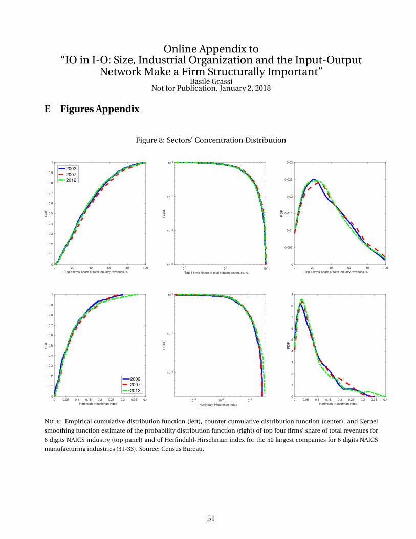
Online Appendix to“IO in I-O: Size, Industrial Organization and the Input-Output

Network Make a Firm Structurally Important”Basile Grassi

Not for Publication. January 2, 2018

E Figures Appendix

Figure 8: Sectors’ Concentration Distribution

0 20 40 60 80 100

Top 4 firms' share of total industry revenues, %

0

0.1

0.2

0.3

0.4

0.5

0.6

0.7

0.8

0.9

1

CD

F

2002

2007

2012

10 0 10 1 10 2

Top 4 firms' share of total industry revenues, %

10 -3

10 -2

10 -1

10 0C

CD

F

0 20 40 60 80 100

Top 4 firms' share of total industry revenues, %

0

0.005

0.01

0.015

0.02

0.025

0.03

PD

F

0 0.05 0.1 0.15 0.2 0.25 0.3 0.35 0.4

Herfindahl-Hirschman index

0

0.1

0.2

0.3

0.4

0.5

0.6

0.7

0.8

0.9

1

CD

F

2002

2007

2012

10 -3 10 -2 10 -1

Herfindahl-Hirschman index

10 -2

10 -1

10 0

CC

DF

0 0.05 0.1 0.15 0.2 0.25 0.3 0.35 0.4

Herfindahl-Hirschman index

0

1

2

3

4

5

6

7

8

9

PD

F

NOTE: Empirical cumulative distribution function (left), counter cumulative distribution function (center), and Kernel

smoothing function estimate of the probability distribution function (right) of top four firms’ share of total revenues for

6 digits NAICS industry (top panel) and of Herfindahl-Hirschman index for the 50 largest companies for 6 digits NAICS

manufacturing industries (31-33). Source: Census Bureau.

51

Figure 9: Sector Concentration

0 10 20 30 40 50 60 70 80 90 100

Top 4 firms' share of total industry revenues 2002, %

0

10

20

30

40

50

60

70

80

90

100

To

p 4

firm

s' s

ha

re o

f to

tal in

du

str

y r

eve

nu

es 2

00

7,

%

22 Utilities

42 Wholesale Trade

44-45 Retail Trade

48-49 Transportation and Warehousing

51 Information

52 Finance and Insurance

53 Real Estate and Rental and Leasing

54 Professional, Scientific

56 Administrative and Support

61 Educational Services

62 Health Care

71 Arts, Entertainment, and Recreation

72 Accommodation and Food Services

81 Other Services

31-33 Manufacturing

0 0.05 0.1 0.15 0.2 0.25 0.3

Herfindahl-Hirschman index (50 largest firms) in 2002, %

0

0.05

0.1

0.15

0.2

0.25

0.3

He

rfin

da

hl-H

irsch

ma

n in

de

x (

50

la

rge

st

firm

s)

in 2

00

7,

%

NOTE: Top Panel: Top four firms’ share of total revenues in 2002 and in 2007 for 6-digit NAICS industry. The mean value is

35.37% in 2002 and 37.21% in 2007. 970 industries. Bottom Panel: Herfindahl-Hirschman-Index for the 50 largest compa-

nies in 2002 and in 2007 for 6 digits NAICS manufacturing industry (31-33). 448 industries. Source: Census Bureau.

52

Figure 10: Approximation of Firms’ Sales Share (Slope)

0 0.05 0.1 0.15 0.2

Sales Share

0.65

0.7

0.75

0.8

0.85

0.9

0.95

1Slope

Bertrand

Approx 2nd

Approx 3rd

0 0.05 0.1 0.15 0.2

Sales Share

0

1

2

3

4

5

6

7

8

9

Deviation

NOTE: For εk = 5. The left panel shows the slope of Bertrand sales share, the slopes of the second and the third order

approximation in Proposition 2 as a function of the monopolistic sales share. The right panel shows percentage deviation

of the slope of both approximations with respect to the numerical solution.

Figure 11: Approximation of Firms’ Sales Share (Different εk)

0 0.05 0.1 0.15 0.2

Sales Share

0

0.02

0.04

0.06

0.08

0.1

0.12

0.14

0.16

0.18

SalesShare

Bertrand

Approx 2nd

0 0.05 0.1 0.15 0.2

Sales Share

0

0.2

0.4

0.6

0.8

1

1.2

1.4

1.6

1.8

Deviation

εk =7

εk =6

εk =5

εk =4

εk =3

NOTE: For different values of εk. The left panel shows the Bertrand sales share using a numerical solver (solid) and the

second order approximation (dashed) as a function of the monopolistic sales share. The right panel shows percentage

deviation of the second order approximation with respect to the numerical solution.

53

Figure 12: Approximation of Firms’ Sales Share (Slope for Different εk)

0 0.05 0.1 0.15 0.2

Sales Share

0.65

0.7

0.75

0.8

0.85

0.9

0.95

1

Slope

Bertrand

Approx 2nd

0 0.05 0.1 0.15 0.2

Sales Share

0

1

2

3

4

5

6

7

Deviation

εk =7

εk =6

εk =5

εk =4

εk =3

NOTE: For different values of εk. The left panel shows the slope of Bertrand sales share (solid) and the slopes of the sec-

ond order approximation (solid) in Proposition 2 as a function of the monopolistic sales share. The right panel shows

percentage deviation of the slope of both approximations with respect to the numerical solution.

54

F Proof Appendix

F.1 Proof of Proposition 3 (Size-Volatility)

Let us first compute the variance of the growth rate of productivity. Let us call nt,k,i the integer such thatproductivity level of firm i in sector k is such that Zt(k, i) = ϕ

nt,k,i

k . Note that Zt(k, i) follows the Markovianprocess described in Assumption 1, therefore its growth rate satisfies:

Zt+1(k, i)− Zt(k, i)

Zt(k, i)=ϕnt+1,k,i

k − ϕnt,k,i

k

ϕnt,k,i

k

= ϕnt+1,k,i−nt,k,i

k − 1 =

ϕ−1k − 1 a

0 with proba b

ϕk − 1 c

Let us compute conditional expected growth rate of the productivity of firm i in sector k:

Et

[Zt+1(k, i)− Zt(k, i)

Zt(k, i)

]= a

(ϕ−1k − 1

)+ c (ϕk − 1) = aϕ−1

k + b+ cϕk − 1

while the conditional variance of the growth rate of Zt(k, i) is

Vart

[Zt+1(k, i)− Zt(k, i)

Zt(k, i)

]= a

(ϕ−1k − 1

)2+ c (ϕk − 1)2 − (aϕ−1

k + b+ cϕk − 1)2 = σ2k

These conditional moments are independent of the level Zt(k, i) at time t and they are equal to their uncondi-tional counterpart. This complete the first part of the proof.

Let us now turn to the growth rate of the sales share st(k, i) of firm i in sector k. To this end, I am using theapproximation in Assumption 2. The first step is to find the growth rate of sales share under monopolistic

competition st(k, i). Note that st(k, i) ∝ Zt(k, i)−γk(1−εk). Keeping sectors’ price and the wage constant, at the

first order we have gs(k,i)t+1 = −γk(1 − εk)g

Z(k,i)t+1 where gxt+1 = xt+1−xt

xt.29 Let us focus on the case of Bertrand

competition. All the following calculation are very similar under Cournot. Thanks to Assumption 2, the salesshare of firm i in sector k is such that st(k, i) = st(k, i)− (1 − ε−1

k )st(k, i)2 which becomes

gs(k,i)t+1 =

st(k, i)

st(k, i)gs(k,i)t+1 − 2

(1− ε−1k )st(k, i)

2

st(k, i)gs(k,i)t+1

Using the fact that gs(k,i)t+1 = −γk(1 − εk)g

Z(k,i)t+1 and after some simplification, we have

gs(k,i)t+1 =γk(εk − 1)

1− 2(1− ε−1k )st(k, i)

1− (1− ε−1k )st(k, i)

gZ(k,i)t+1

The conditional variance of the growth rate of firm i in sector k is

Vart

[st+1(k, i)− st(k, i)

st(k, i)

]=γ2k(εk − 1)2

(1− 2(1− ε−1

k )st(k, i)

1− (1− ε−1k )st(k, i)

)2

σ2k

The above equation shows that the variance of the growth rate of the sales share of a firm is a strictly decreasing

function of its level. Indeed the function gk : x 7→ γ2k(εk − 1)21−2(1−ε−1

k )x

1−(1−ε−1k )x

is strictly decreasing and the absolute

value of its slope |g′k(x)| = γ2k(εk − 1)2(1−ε−1

k )

(1−(1−ε−1k )x)2

is strictly increasing in εk.

F.2 Proof of Proposition 6 (Sector k’s Productivity Distribution Dynamics)

In this section, I first derive equation 4 before solving for the stationary distribution in sector k.

29Equivalently, one can compute this growth rate under the stationary equilibrium, the steady-state of this economywhere aggregate and sectoral quantities and prices are constant (as if they were a continuum of sectors).

55

Proof of Equation 4: For n such that 0 < n < Mk, Assumption 1 implies that

g(k)t+1,n = fn,n−1

k,t+1 + fn,nk,t+1 + fn,n+1

k,t+1

where fn′,nk,t+1 is the number of firms in productivity bin n′ at t + 1 that were in bin n at time t. Thanks to

Assumption 1 the 3× 1 vector f .,nk,t+1 = (fn−1,n

k,t+1 , fn,nk,t+1, f

n+1,nk,t+1 )′ follow a multinomial distribution with number

of trial g(k)t,n and event probabilities (ak, bk, ck)

′. It follows that the 3 × 1 vector f .,nk,t+1 has a mean Et

[f .,nk,t+1

]=

g(k)t,n (ak, bk, ck)

′ and a variance-covariance matrix equal to g(k)t,nΣk where

Σk =

(ak(1− ak) −akbk −akck−akbk bk(1 − bk) −bkck−akck −bkck ck(1 − ck)

)

Note that f .,nk,t+1 are independent across n and thus

Et

[g(k)t+1,n

]= Et

[fn,n−1k,t+1

]+ Et

[fn,nk,t+1

]+ Et

[fn,n+1k,t+1

]= akg

(k)t,n+1 + bkg

(k)t,n + ckg

(k)t,n−1

Vart[g(k)t+1,n

]= Vart

[fn,n−1k,t+1

]+ Vart

[fn,nk,t+1

]+ Vart

[fn,n+1k,t+1

]= ak(1− ak)g

(k)t,n+1 + bk(1− bk)g

(k)t,n + ck(1− ck)g

(k)t,n−1

For completeness, let us look at the covariance structure of the g(k)t+1,n:

Covt[g(k)t+1,n; g

(k)t+1,n′

]= Covt

[fn,n−1k,t+1 + fn,n

k,t+1 + fn,n+1k,t+1 ; fn′,n′−1

k,t+1 + fn′,n′

k,t+1 + fn′,n′+1k,t+1

]= 0 if |n− n′| > 2

since the f .,nk,t+1 are independent across n. For n′ = n+ 1, we have:

Covt

[g(k)t+1,n; g

(k)t+1,n+1

]= Covt

[fn,n−1k,t+1 + fn,n

k,t+1 + fn,n+1k,t+1 ; fn+1,n

k,t+1 + fn+1,n+1k,t+1 + fn+1,n+2

k,t+1

]

= Covt

[fn,nk,t+1; f

n+1,nk,t+1

]+ Covt

[fn,n+1k,t+1 ; fn+1,n+1

k,t+1

]

= −bkckg(k)t,n − akbkg(k)t,n+1

using the fact the variance-covariance matrix of f .,nk,t+1 is equal to µ

(k)t,nΣk for all n > 0. The same reasoning

apply for n′ = n+ 2.For n = 0, Assumption 1 implies

g(k)t+1,0 = f0,0

k,t+1 + f0,1k,t+1

and that the 2 × 1 vector f .,0k,t+1 = (f0,0

k,t+1, f1,0k,t+1)

′ follow a multinomial distribution with number of trial g(k)t,0

and event probabilities (ak + bk, ck)′. The same reasoning than for n > 0 applies.

For n =Mk, Assumption 1 implies

g(k)t+1,M = fM,M−1

k,t+1 + fM,Mk,t+1

and that the 2× 1 vector f .,Mk,t+1 = (fM−1,M

k,t+1 , fM,Mk,t+1)

′ follow a multinomial distribution with number of trial g(k)t,M

and event probabilities (ak, ck + bk)′. The same reasoning than for n > 0 applies.

Gathering the above results we have in matrix form:

g(k)t+1 = (P(k))′g

(k)t + ǫ

(k)t

where ǫ(k)t is the M × 1 vector of ǫ

(k)t,n. This complete the derivation of Equation 4.

Stationary Distribution in Sector k: Let us drop the (k) superscript and subscript to simplify notation.The stationary distribution is a sequence that solve the following system:

(BC1) g0 = (a+ b)g0 + ag1

(BC2) gM = cgM−1 + (b+ c)gM

(EH) gn = agn+1 + bgn + cgn−1

Let us solve for the general solution of (EH). This equation is a second order linear difference equation equiv-alent to 0 = agn+1+(b− 1)gn+ cgn−1 = agn+1− (a+ c)gn+ cgn−1, with an associated second order polynomial

56

aX2 − (a + c)X + c = 0 which have roots 1 and ca

. The general solution of (EH) is thus gn = K1 + K2

(ca

)nwhere K1 and K2 are constant to solve for.Let us substitute this general solution in the equation (BC1), it yields

K1 +K2 = (a+ b)(K1 +K2) + aK1 + aK2c

a= (2a+ b)K1 + (a+ b+ c)K2

since a+b+c = 1, (BC1) impliesK1 = (2a+b)K1. Since a < c and a+b+c = 1, then 2a+b 6= 1 and thusK1 = 0.

The general solution of this system is then gn = K2

(ca

)n. It is trivial to see that (BC2) is satisfied by this general

solution. Since n = logϕn

logϕ, thus

(ca

)n= exp

(−s log a

c

)= exp

(− logϕn

logϕlog a

c

)= (ϕn)

−δwith δ =

log ac

logϕ. It follows

that gn = K2 (ϕn)

−δ

To solve for K2, let us use the fact that gn has to sum to Nk, the number of firms in sector k.

Nk =

M∑

n=0

gn = K2

M∑

n=0

(ϕ−δ

)n= K2

1−(ϕ−δ

)M+1

1− ϕ−δ

since ϕ−δ < 1. It follows that K2 = Nk(1−ϕ−δ)

1−(ϕ−δ)M+1 and g(k)n = Nk

(1−ϕ−δ)

1−(ϕ−δ)M+1 (ϕn)−δ .

F.3 Proof of Proposition 7 (Dynamics of Zt,k and ∆t,k)

Let us defineMZt,k(ξ) =∑Nk

i=1 Zt(k, i)ξ the ξth moment of the productivity distribution within sector k at time

t. Note that since productivity evolves on the discrete state spaceΦk = 1, ϕk, · · · , ϕnk , · · · , ϕMk

k , we can rewrite

MZt,k(ξ) =∑Nk

i=1 Zt(k, i)ξ =

∑Nk

i=1 ϕξnt,k,i

k where nt,k,i is such that the firm i in sector k has a productivity level

ϕnt,k,i at time t. It follows that MZt,k(ξ) =∑Mk

n=0(ϕnk )

ξg(k)t,n by instead of summing over firms i, summing over

productivity level ϕnk . Below, I am showing two lemmas that totally described the dynamics of the moments

MZt,k(ξ) for any ξ. With these results in hand I am then characterizing the dynamics of the two moments of

interest: Zt,k and ∆t,k.

Lemma 4 (Dynamics of Moments of the Productivity Distribution) Under Assumption 1, the ξth moment of

the productivity distribution within sector k,MZt,k(ξ) =∑Nk

i=1 Z(k, i)ξ, satisfies

MZt+1,k(ξ) = ρk(ξ)MZt,k(ξ) +OMt,k(ξ) + σt,k(ξ)εt

σt,k(ξ)2 = k(ξ)MZt,k(2ξ) +Oσ

t,k(ξ)

where εt is an iid (across t and k) random variable following a N (0, 1), where ρk(ξ) = akϕ−ξk + bk + ckϕ

ξk, and

where k(ξ) = akϕ−2ξk + bk + ckϕ

2ξk − ρk(ξ)

2.

Proof of Lemma 4: Note first that

MZt+1,k(ξ) =

Nk∑

i=1

Zt+1(k, i)ξ =

Nk∑

i=1

ϕξnt+1,k,i

k =

Mk∑

n=0

(ϕnk )

ξg(k)t+1,n

where g(k)t+1,n is a stochastic as shown in Proposition 6. In the proof of this proposition we have shown that for

n such that 0 < n < Mk

g(k)t+1,n = fn,n−1

k,t+1 + fn,nk,t+1 + fn,n+1

k,t+1

where fn′,nk,t+1 is the number of firms in productivity bin n′ at t+1 that were in bin n at time t. Given assumption

1 the 3 × 1 vector f .,nk,t+1 = (fn−1,n

k,t+1 , fn,nk,t+1, f

n+1,nk,t+1 )′ follow a multinomial distribution with number of trial g

(k)t,n

and event probabilities (ak, bk, ck)′. In other words,

f .,nk,t+1 =

(fn−1,nk,t+1

fn,nk,t+1

fn+1,nk,t+1

) Multi

(µ(k)t,n ,( ak

bkck

))

57

Severini (2005) (p377 example 12.7) shows that a multinomial distribution can be approximate (i.e convergein distribution) by a multivariate normal distribution:

1√g(k)t,n

(f .,nk,t+1 − g

(k)t,n

( ak

bkck

))D−→

g(k)t,n→∞

Z N (0,Σk)

where Σk =

(ak(1− ak) −akbk −akck−akbk bk(1− bk) −bkck−akck −bkck ck(1− ck)

).

For n = 0, thanks to Assumption 1 g(k)t+1,0 = f0,0

k,t+1 + f0,1k,t+1 and the 2 × 1 vector f .,0

k,t+1 = (f0,0k,t+1, f

1,0k,t+1)

′

follow a multinomial distribution with number of trial g(k)t,0 and event probabilities (ak + bk, ck)

′. Using

the same result in Severini (2005), 1√

g(k)t,0

(f .,0k,t+1 − g

(k)t,0

(ak+bk

ck

)) D−→g(k)t,0 →∞

Z N (0,Σ(0)k ) where Σ

(0)k =

(ck(1− ck) −ck(1− ck)−ck(1− ck) ck(1 − ck)

).

For n = Mk, thanks to Assumption 1 g(k)t+1,0 = fM,M

k,t+1 + fM,M−1k,t+1 and the 2 × 1 vector f .,M

k,t+1 = (fM−1,Mk,t+1 , fM,M

k,t+1)′

follow a multinomial distribution with number of trial g(k)t,M and event probabilities (ak, bk + ck)

′. Using

the same result in Severini (2005), 1√

g(k)t,0

(f .,Mk,t+1 − g

(k)t,M

( ak

bk+ck

)) D−→g(k)t,M→∞

Z N (0,Σ(M)k ) where Σ

(M)k =

(ak(1− ak) −ak(1 − ak)−ak(1− ak) ak(1− ak)

).

Let us keep these results in mind and let us go back to (I drop the subscript k to keep the notation parsimo-nious)

MZt+1,k(ξ) =

M∑

n=0

(ϕn)ξG(k)t+1,n = g

(k)t+1,0 +

M−1∑

n=1

(ϕn)ξg(k)t+1,n + (ϕM )ξg

(k)t+1,M

= f0,0k,t+1 + f0,1

k,t+1 +

M−1∑

n=1

(ϕn)ξ(fn,n−1k,t+1 + fn,n

k,t+1 + fn,n+1k,t+1

)+ (ϕM )ξ

(fM,M−1k,t+1 + fM,M

k,t+1

)

= f0,0k,t+1 + f0,1

k,t+1 +M−1∑

n=1

(ϕξ)nfn,n−1k,t+1 +

M−1∑

n=1

(ϕξ)nfn,nk,t+1 +

M−1∑

n=1

(ϕξ)nfn,n+1k,t+1 + (ϕM )ξ

(fM,M−1k,t+1 + fM,M

k,t+1

)

= f0,0k,t+1 + f0,1

k,t+1 +M−2∑

n=0

(ϕξ)n+1fn+1,nk,t+1 +

M−1∑

n=1

(ϕξ)nfn,nk,t+1 +

M∑

n=2

(ϕξ)n−1fn−1,nk,t+1 + (ϕM )ξ

(fM,M−1k,t+1 + fM,M

k,t+1

)

= f0,0k,t+1 + ϕξf1,0

k,t+1 +

M−1∑

n=1

(ϕξ)n(ϕξfn+1,n

k,t+1 + fn,nk,t+1 + ϕ−ξ + fn−1,n

k,t+1

)+ (ϕξ)M

(fM,Mk,t+1 + ϕ−ξfM−1,M

k,t+1

)

=(

1ϕξ

)′ ( f0,0k,t+1

f1,0k,t+1

)+

M−1∑

n=1

(ϕξ)n(

ϕ−ξ

1ϕξ

)′

fn−1,nk,t+1

fn,nk,t+1

fn+1,nk,t+1

+ (ϕξ)M

(ϕ−ξ

1

)′( fM−1,Mk,t+1

fM,Mk,t+1

)

=

(ρk,0g

(k)t,0 +

√k,0g

(k)t,0 εt+1,0

)+

M−1∑

n=1

(ϕξ)n(ρkg

(k)t,n +

√kg

(k)t,nεt+1,n

). . .

. . .+ (ϕξ)M(ρk,Mg

(k)t,M +

√k,Mg

(k)t,nεt+1,M

)

Since

(fn−1,nk,t+1

fn,nk,t+1

fn+1,nk,t+1

)≈ Z N

(g(k)t,n

( ak

bkck

), g

(k)t,nΣk

)it follows that

(ϕ−ξ

1ϕξ

)′(

fn−1,nk,t+1

fn,nk,t+1

fn+1,nk,t+1

)≈

(ϕ−ξ

1ϕξ

)′

Z

N(g(k)t,n

(x−ξ

1xξ

)′ ( ak

bkck

), g

(k)t,n

(x−ξ

1xξ

)′

Σ

(ϕ−ξ

1ϕξ

))= N

(g(k)t,nρk, g

(k)t,nk

). where ρk = akϕ

−ξ + bk + ckϕξ and

k = akϕ−2ξ+bk+ckϕ

2ξ−ρ2k. The same reasoning apply for n =Mk with ρk,M = ρk+c(1−ϕξ) := ρk+ ρk,M and

k,M = k − c(1− c)(1− x2ξ)− 2cb(1−ϕξ)− 2ca(1−ϕξ) := k + ˜k,M . The same reasoning apply for n = 0 with

ρk,0 = ρk + a(1−ϕ−ξ) := ρk + ρk,0 and k,0 = k − a(1− a)(1− x−2ξ)− 2ab(1−ϕ−ξ)− 2ac(1−ϕ−ξ) := k + ˜k,0.

58

From this it follows that

MZt+1,k(ξ) =(ρk,0g

(k)t,0

)+ ρk

M∑

n=0

(ϕξ)ng(k)t,n + (ϕξ)M

(ρk,Mg

(k)t,M

)+ σt,k(ξ)εt+1

= ρk(ξ)MZt,k(ξ) +OMt,k(ξ) + σt,k(ξ)εt+1

Where OMt,k(ξ) = ρk,0g

(k)t,0 + (ϕξ)M ρk,Mg

(k)t,M .Since the εt+1,n are independent across n, the variance of σt,k(ξ)εt

is the sum of the variances of

√kg

(k)t,nεt+1,n i.e

σt,k(ξ)2 = k,0g

(k)t,0 +

M−1∑

n=1

(ϕ2ξ)nkg(k)t,n + (ϕ2ξ)Mk,Mg

(k)t,n

= (k + ˜k,0) g(k)t,0 +

M−1∑

n=1

(ϕ2ξ)nkg(k)t,n + (ϕ2ξ)M (k + ˜k,M ) g

(k)t,n

= ˜k,0g(k)t,0 +M∑

n=0

(ϕ2ξ)nkg(k)t,n + (ϕ2ξ)M ˜k,Mg(k)t,n

= k(ξ)MZt,k(2ξ) +Oσt,k(ξ)

where Oσt,k(ξ) = ˜k,0g(k)t,0 + (ϕ2ξ)M ˜k,Mg(k)t,n . Moreover, εt+1 follows a standard normal distribution since the

εt+1,n are also normally distributed.

Lemma 5 (Covariance of Moments of the Productivity Distribution) Under Assumption 1, the covariance be-tween the ξth moment and the ξ′th moment of the productivity distribution within sector k is given by

Covt [MZt+1,k(ξ);MZt+1,k(ξ′)] = k(ξ, ξ

′)MZt,k(ξ′ + ξ) +OC

t,k(ξ, ξ′)

where MZt,k(ξ) =∑Nk

i=1 Z(k, i)ξ and k(ξ, ξ

′) = ak(1− ak)ϕ−(ξ+ξ′)k + bk(1− bk) + ck(1− ck)ϕ

ξ+ξ′

k − akbk(ϕ−ξk +

ϕ−ξ′

k )− akck(ϕ−(ξ−ξ′)k ϕξ−ξ′

k )− bkck(ϕξk + ϕξ′

k ).

Proof of Lemma 5: In the proof of Lemma 4, we had

MZt+1,k(ξ) =(

1ϕξ

)′( f0,0k,t+1

f1,0k,t+1

)+

M−1∑

n=1

(ϕξ)n(

ϕ−ξ

1ϕξ

)′(

fn−1,nk,t+1

fn,nk,t+1

fn+1,nk,t+1

)+ (ϕξ)M

(ϕ−ξ

1

)′( fM−1,Mk,t+1

fM,Mk,t+1

)

Here I drop the subscript k to keep the notation simpler. Let us compute the covariance between two momentsof the productivity distribution in sector k:

Covt

[

MZt+1,k(ξ);MZt+1,k(ξ′)]

=Covt

(

1

ϕξ

)

′

f0,0k,t+1

f1,0k,t+1

+

M−1∑

n=1

(ϕξ)n

(

ϕ−ξ

1

ϕξ

)

′

fn−1,nk,t+1

fn,nk,t+1

fn+1,nk,t+1

+ (ϕξ)M(

ϕ−ξ

1

)

′

fM−1,Mk,t+1

fM,Mk,t+1

;

(

1

ϕξ′

)

′

f0,0k,t+1

f1,0k,t+1

+

M−1∑

n=1

(ϕξ′

)n

ϕ−ξ′

1

ϕξ′

′

fn−1,nk,t+1

fn,nk,t+1

fn+1,nk,t+1

+ (ϕξ′

)M(

ϕ−

1

=Covt

(

1

ϕξ

)

′

f0,0k,t+1

f1,0k,t+1

;

(

1

ϕξ′

)

′

f0,0k,t+1

f1,0k,t+1

+

M−1∑

n=1

M−1∑

n′=1

(ϕξ)n(ϕ

ξ′)n′

Covt

(

ϕ−ξ

1

ϕξ

)

′

fn−1,nk,t+1

fn,nk,t+1

fn+1,nk,t+1

;

ϕ−ξ′

1

ϕξ′

′

fn′

−1,n′

k,t+1

fn′,n′

k,t+1

fn′+1,n′

k,t+1

+ . . .

. . . + (ϕξ+ξ′

)M

Covt

(

ϕ−ξ

1

)

′

fM−1,Mk,t+1

fM,Mk,t+1

;

(

ϕ−ξ′

1

)

′

fM−1,Mk,t+1

fM,Mk,t+1

=Covt

(

1

ϕξ

)

′

f0,0k,t+1

f1,0k,t+1

;

(

1

ϕξ′

)

′

f0,0k,t+1

f1,0k,t+1

+

M−1∑

n=1

(ϕξ+ξ′

)nCovt

(

ϕ−ξ

1

ϕξ

)

′

fn−1,nk,t+1

fn,nk,t+1

fn+1,nk,t+1

;

ϕ−ξ′

1

ϕξ′

′

fn−1,nk,t+1

fn,nk,t+1

fn+1,nk,t+1

. . .

. . . + (ϕξ+ξ′

)M

Covt

(

ϕ−ξ

1

)

′

fM−1,Mk,t+1

fM,Mk,t+1

;

(

ϕ−ξ′

1

)

′

fM−1,Mk,t+1

fM,Mk,t+1

where at the second line, we use the fact that f .,0k,t+1 and f .,M

k,t+1 are independent of the f .,nk,t+1 for any 0 < n < M

and in the third line that f .,nk,t+1 are independent across n. Using the fact that Cov[A′X,B′Y ] = A′

Cov[X,Y ]B

59

for vectorsA and B and random vectorsX and Y of appropriate size, we have

Covt

[

MZt+1,k(ξ);MZt+1,k(ξ′)]

=

(

1

ϕξ

)

′

Covt

f0,0k,t+1

f1,0k,t+1

;

f0,0k,t+1

f1,0k,t+1

(

1

ϕξ′

)

+

M−1∑

n=1

(ϕξ+ξ′

)n

(

ϕ−ξ

1

ϕξ

)

′

Covt

fn−1,nk,t+1

fn,nk,t+1

fn+1,nk,t+1

;

fn−1,nk,t+1

fn,nk,t+1

fn+1,nk,t+1

ϕ−ξ′

1

ϕξ′

. . .

. . . + (ϕξ+ξ′

)M(

ϕ−ξ

1

)

′

Covt

fM−1,Mk,t+1

fM,Mk,t+1

;

fM−1,Mk,t+1

fM,Mk,t+1

(

ϕ−ξ′

1

)

Using the definition of Σ, Σ(0) and Σ(M) yields

Covt [MZt+1,k(ξ);MZt+1,k(ξ′)] =

g(k)t,0

(1ϕξ

)′Σ(0)

(1

ϕξ′

)+

M−1∑

n=1

(ϕξ+ξ′)ng(k)t,n

(ϕ−ξ

1ϕξ

)′

Σ

(ϕ−ξ′

1

ϕξ′

)+ (ϕξ+ξ′)Mg

(k)t,M

(ϕ−ξ

1

)′Σ(M)

(ϕ−ξ′

1

)

To complete the proof, let us just note that

(

ϕ−ξ

1ϕξ

)′

Σ

(

ϕ−ξ′

1

ϕξ′

)

= a(1 − a)ϕ−(ξ+ξ′) + b(1 − b) + c(1− c)ϕξ+ξ′ − ab(ϕ−ξ + ϕ−ξ′ )− ac(ϕ−(ξ−ξ′)ϕξ−ξ′ )− bc(ϕξ + ϕξ′ )

(

1ϕξ

)′Σ(0)

(

1

ϕξ′

)

= c(1− c)(1 − ϕξ′ − ϕξ + ϕξ+ξ′ )

(

ϕ−ξ

1

)′Σ(M)

(

ϕ−ξ′

1

)

= a(1 − a)(1 − ϕ−ξ′ − ϕ−ξ + ϕ−(ξ+ξ′))

which implies that

OCt,k(ξ, ξ

′)

= g(k)t,0

((ϕ−ξ

1ϕξ

)′

Σ

(ϕ−ξ′

1

ϕξ′

)−(

1ϕξ

)′Σ(0)

(1

ϕξ′

))+ (ϕξ+ξ′ )Mg

(k)t,M

((ϕ−ξ

1ϕξ

)′

Σ

(ϕ−ξ′

1

ϕξ′

)−(

ϕ−ξ

1

)′Σ(M)

(ϕ−ξ′

1

))

= g(k)t,0 k,0 + (ϕξ+ξ′ )Mg

(k)t,Mk,M

Proof of Proposition 7: Using Lemma 4 and the fact that Zt,k = MZt,k

((εk − 1)γk

)and that ∆t,k =

Zt,k2MZt,k

(2(εk − 1)γk

), we have

Zt+1,k = ρ(Z)k Zt,k + o

(Z)t,k +

√(Z)k ∆t,k +O

(Z)t,k Zt,k ε

(Z)t+1,k

(Zt+1,k

Zt,k

)2

∆t+1,k = ρ(∆)k ∆t,k + o

(∆)t,k +

√(∆)k κt,k +O

(∆)t,k ∆t,k ε

(∆)t+1,k

Finally, Lemma 5 shows that the covariance Covt

[ε(1)t+1; ε

(2)t+1

]6= 0.

60