Invited Review Article: IceCube: An instrument for neutrino … · Invited Review Article: IceCube:...
24
Invited Review Article: IceCube: An instrument for neutrino astronomy Francis Halzen 1 and Spencer R. Klein 2 1 Department of Physics, University of Wisconsin, 1150 University Avenue, Madison, Wisconsin 53706, USA 2 Nuclear Science Division, Lawrence Berkeley National Laboratory, Berkeley, California 94720, USA and Department of Physics, University of California, Berkeley, California 94720, USA Received 30 March 2010; accepted 5 July 2010; published online 30 August 2010 Neutrino astronomy beyond the Sun was first imagined in the late 1950s; by the 1970s, it was realized that kilometer-scale neutrino detectors were required. The first such instrument, IceCube, is near completion and taking data. The IceCube project transforms 1 km 3 of deep and ultra- transparent Antarctic ice into a particle detector. A total of 5160 optical sensors is embedded into a gigaton of Antarctic ice to detect the Cherenkov light emitted by secondary particles produced when neutrinos interact with nuclei in the ice. Each optical sensor is a complete data acquisition system including a phototube, digitization electronics, control and trigger systems, and light-emitting diodes for calibration. The light patterns reveal the type flavor of neutrino interaction and the energy and direction of the neutrino, making neutrino astronomy possible. The scientific missions of IceCube include such varied tasks as the search for sources of cosmic rays, the observation of galactic supernova explosions, the search for dark matter, and the study of the neutrinos themselves. These reach energies well beyond those produced with accelerator beams. The outline of this review is as follows: neutrino astronomy and kilometer-scale detectors, high-energy neutrino telescopes: methodologies of neutrino detection, IceCube hardware, high-energy neutrino telescopes: beyond astronomy, and future projects. © 2010 American Institute of Physics. doi:10.1063/1.3480478 I. INTRODUCTION A. The technology Soon after the 1956 observation of the neutrino, 1 the idea emerged that it represented the ideal astronomical messenger. Neutrinos travel from the edge of the Universe essentially without absorption and with no deflection by magnetic fields. Having essentially no mass and no electric charge, the neu- trino is similar to the photon, except for one important at- tribute: its interactions with matter are extremely feeble. So, high-energy neutrinos may reach us unscathed from cosmic distances, from the inner neighborhood of black holes, and, hopefully, from the nuclear furnaces where cosmic rays are born. Also, in contrast to photons, neutrinos are an unam- biguous signature of hadronic interactions. Their weak interactions make cosmic neutrinos very dif- ficult to detect. Immense particle detectors are required to collect cosmic neutrinos in statistically significant numbers. 2 By the 1970s, it was clear that a cubic-kilometer detector was needed to observe cosmic neutrinos produced by the interactions of cosmic rays with background microwave photons. 3 Newer estimates for observing potential cosmic ac- celerators such as quasars or gamma-ray bursts unfortunately point to the same exigent requirement. 4 Building a neutrino telescope has been a daunting technical challenge. Given the detector’s required size, early efforts concen- trated on transforming large volumes of natural water into Cherenkov detectors that catch the light produced when neu- trinos interact with nuclei in or near the detector. 5 Building the Deep Underwater Muon and Neutrino Detector DUMAND in the sea off the main island of Hawaii unfor- tunately failed after a two-decade-long effort. 6 However, DUMAND paved the way for later efforts by pioneering many of the detector technologies in use today and by inspir- ing the deployment of a smaller instrument in Lake Baikal, 7 as well as efforts to commission neutrino telescopes in the Mediterranean. 8–10 The first telescope on the scale envisaged by the DUMAND collaboration was realized instead by transforming a large volume of the extremely transparent, natural deep Antarctic ice into a particle detector, the Antarc- tic Muon and Neutrino Detector Array AMANDA. In op- eration from 2000 to 2009, it represented a proof of concept for the kilometer-scale neutrino observatory, IceCube, which is the main focus of this article. 11,12 Even extremely high-energy neutrinos will routinely stream through a detector without leaving a trace; the few that interact with a nucleus in the ice create muons as well as electromagnetic and hadronic secondary particle showers. The charged secondary particles radiate Cherenkov light that spreads through the transparent ice characterized by an ab- sorption length of 100 m or more, depending on depth. The light pattern reveals the direction of the neutrino, making neutrino astronomy possible. Secondary muons are of special interest because their mean free path can reach 10 km for the most energetic neutrinos. The effective detector volume thus exceeds the instrumented volume for muon neutrinos. The method is illustrated in Fig. 1a. Photomultipliers transform the Cherenkov light from neutrino interactions into electrical signals using the photo- electric effect. These signals are captured by computer chips that digitize the shape of the current pulses. The information is sent to the computers collecting the data, first by cable to the “counting house” at the surface of the ice sheet and then REVIEW OF SCIENTIFIC INSTRUMENTS 81, 081101 2010 0034-6748/2010/818/081101/24/$30.00 © 2010 American Institute of Physics 81, 081101-1
-
Upload
truongngoc -
Category
Documents
-
view
217 -
download
0
Transcript of Invited Review Article: IceCube: An instrument for neutrino … · Invited Review Article: IceCube:...
Invited Review Article: IceCube: An instrument for neutrino astronomyFrancis Halzen1 and Spencer R. Klein2
1Department of Physics, University of Wisconsin, 1150 University Avenue, Madison, Wisconsin 53706, USA2Nuclear Science Division, Lawrence Berkeley National Laboratory, Berkeley, California 94720, USAand Department of Physics, University of California, Berkeley, California 94720, USA
�Received 30 March 2010; accepted 5 July 2010; published online 30 August 2010�
Neutrino astronomy beyond the Sun was first imagined in the late 1950s; by the 1970s, it wasrealized that kilometer-scale neutrino detectors were required. The first such instrument, IceCube, isnear completion and taking data. The IceCube project transforms 1 km3 of deep and ultra-transparent Antarctic ice into a particle detector. A total of 5160 optical sensors is embedded into agigaton of Antarctic ice to detect the Cherenkov light emitted by secondary particles produced whenneutrinos interact with nuclei in the ice. Each optical sensor is a complete data acquisition systemincluding a phototube, digitization electronics, control and trigger systems, and light-emitting diodesfor calibration. The light patterns reveal the type �flavor� of neutrino interaction and the energy anddirection of the neutrino, making neutrino astronomy possible. The scientific missions of IceCubeinclude such varied tasks as the search for sources of cosmic rays, the observation of galacticsupernova explosions, the search for dark matter, and the study of the neutrinos themselves. Thesereach energies well beyond those produced with accelerator beams. The outline of this review is asfollows: neutrino astronomy and kilometer-scale detectors, high-energy neutrino telescopes:methodologies of neutrino detection, IceCube hardware, high-energy neutrino telescopes: beyondastronomy, and future projects. © 2010 American Institute of Physics. �doi:10.1063/1.3480478�
I. INTRODUCTION
A. The technology
Soon after the 1956 observation of the neutrino,1 the ideaemerged that it represented the ideal astronomical messenger.Neutrinos travel from the edge of the Universe essentiallywithout absorption and with no deflection by magnetic fields.Having essentially no mass and no electric charge, the neu-trino is similar to the photon, except for one important at-tribute: its interactions with matter are extremely feeble. So,high-energy neutrinos may reach us unscathed from cosmicdistances, from the inner neighborhood of black holes, and,hopefully, from the nuclear furnaces where cosmic rays areborn. Also, in contrast to photons, neutrinos are an unam-biguous signature of hadronic interactions.
Their weak interactions make cosmic neutrinos very dif-ficult to detect. Immense particle detectors are required tocollect cosmic neutrinos in statistically significant numbers.2
By the 1970s, it was clear that a cubic-kilometer detectorwas needed to observe cosmic neutrinos produced by theinteractions of cosmic rays with background microwavephotons.3 Newer estimates for observing potential cosmic ac-celerators such as quasars or gamma-ray bursts unfortunatelypoint to the same exigent requirement.4 Building a neutrinotelescope has been a daunting technical challenge.
Given the detector’s required size, early efforts concen-trated on transforming large volumes of natural water intoCherenkov detectors that catch the light produced when neu-trinos interact with nuclei in or near the detector.5 Buildingthe Deep Underwater Muon and Neutrino Detector�DUMAND� in the sea off the main island of Hawaii unfor-tunately failed after a two-decade-long effort.6 However,
DUMAND paved the way for later efforts by pioneeringmany of the detector technologies in use today and by inspir-ing the deployment of a smaller instrument in Lake Baikal,7
as well as efforts to commission neutrino telescopes in theMediterranean.8–10 The first telescope on the scale envisagedby the DUMAND collaboration was realized instead bytransforming a large volume of the extremely transparent,natural deep Antarctic ice into a particle detector, the Antarc-tic Muon and Neutrino Detector Array �AMANDA�. In op-eration from 2000 to 2009, it represented a proof of conceptfor the kilometer-scale neutrino observatory, IceCube, whichis the main focus of this article.11,12
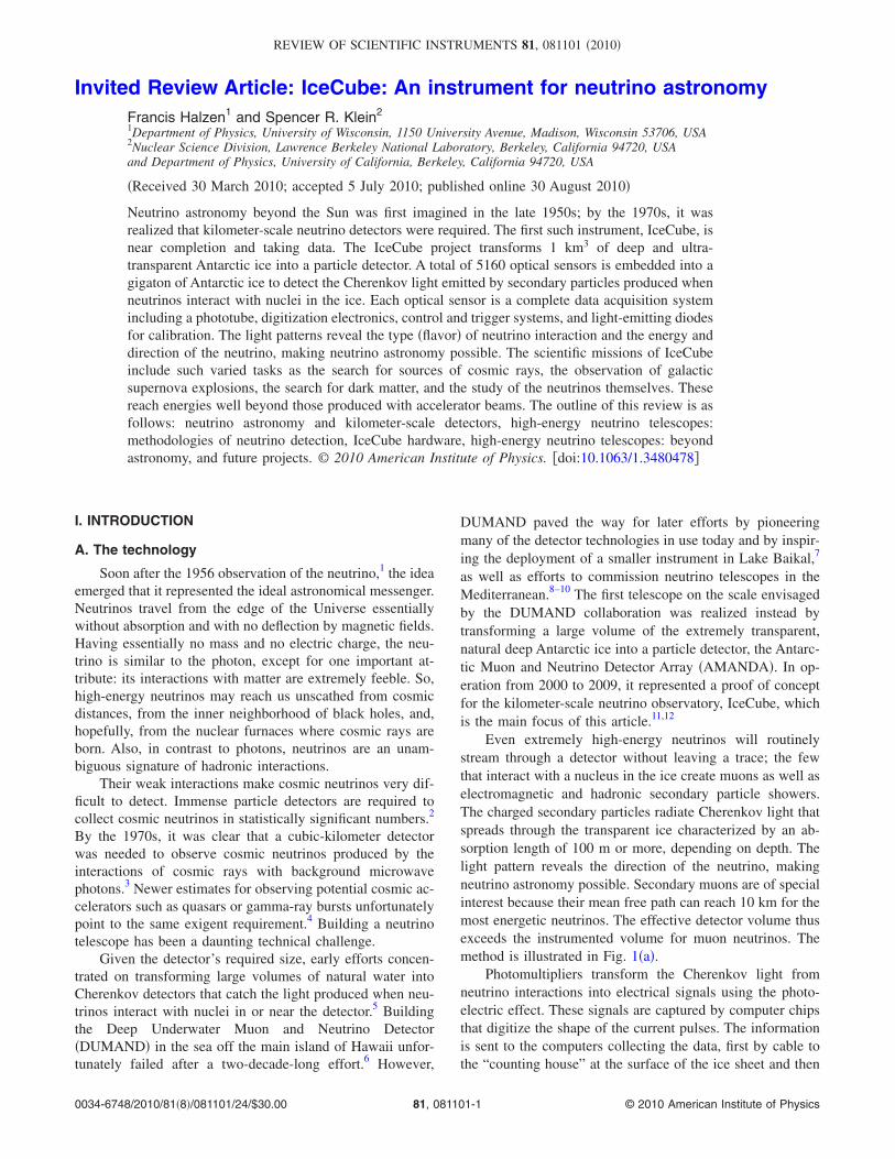
Even extremely high-energy neutrinos will routinelystream through a detector without leaving a trace; the fewthat interact with a nucleus in the ice create muons as well aselectromagnetic and hadronic secondary particle showers.The charged secondary particles radiate Cherenkov light thatspreads through the transparent ice characterized by an ab-sorption length of 100 m or more, depending on depth. Thelight pattern reveals the direction of the neutrino, makingneutrino astronomy possible. Secondary muons are of specialinterest because their mean free path can reach 10 km for themost energetic neutrinos. The effective detector volume thusexceeds the instrumented volume for muon neutrinos. Themethod is illustrated in Fig. 1�a�.
Photomultipliers transform the Cherenkov light fromneutrino interactions into electrical signals using the photo-electric effect. These signals are captured by computer chipsthat digitize the shape of the current pulses. The informationis sent to the computers collecting the data, first by cable tothe “counting house” at the surface of the ice sheet and then
REVIEW OF SCIENTIFIC INSTRUMENTS 81, 081101 �2010�
0034-6748/2010/81�8�/081101/24/$30.00 © 2010 American Institute of Physics81, 081101-1
via magnetic tape. More interesting events are sent by satel-lite to the IceCube data warehouse in Madison, WI. Essen-tially, IceCube consists of 5160 freely running sensors send-ing time-stamped, digitized waveforms of the light theydetect to the surface. The local clocks in the sensors are keptcalibrated with nanosecond precision. This information al-lows the scientists to reconstruct neutrino events and infertheir arrival directions and energies.
The complete IceCube detector will observe several hun-dred neutrinos per day,14,15 with energies above 100 GeV; theDeepCore infill array will identify a smaller sample withenergies as low as 10 GeV. These “atmospheric neutrinos”come from the decay of pions and kaons produced by thecollisions of cosmic-ray particles with nitrogen and oxygenin the atmosphere. Atmospheric neutrinos are a backgroundfor cosmic neutrinos, at least for energies below 1000 TeV,but their flux is calculable and can be used to prove that thedetector is performing as expected. At the highest energy, asmall charm component is anticipated; its magnitude is un-certain and remains to be measured. As in conventional as-tronomy, IceCube looks beyond the atmosphere for cosmicsignals.
In parallel, the development of the technology for com-
missioning a large detector deployed in sea or fresh water �ina lake� continued.16 Water can have excellent optical quality,with a long scattering length that can lead to a very goodangular resolution. The decay of radioactive potassium-40typically contributes a steady 40 kHz background rate in a10 in. photomultiplier tube �PMT�. Bioluminescence alsocontributes bursts of background light that result in detectordead time. Currents are also an issue; it is necessary to trackthe position of the optical sensors. In contrast, Antarctic icehas a shorter scattering length than water, but the attenuationlength is longer. With appropriate reconstruction algorithms,it is possible to place the optical sensors farther apart in icethan in water. Furthermore, the only background in the sterileice is that introduced by the detector itself.
As has already been mentioned, the original effort tobuild a large detector was by the DUMAND collaboration.6
They proposed to build a substantial deep-ocean detector at asite about 40 km off the coast of the island of Hawaii, in4800 m of water. Buoyant strings of PMTs were to be an-chored to the seabed and connected to the shore by an un-derwater cable. The challenges were formidable for the1980s technology: high pressures, corrosive salt water andlarge backgrounds from bioluminescence, and radioactive40K. DUMAND was canceled after a pressure vessel leakedduring the very first string deployment.
Another effort by a Russian and German collaboration inLake Baikal, in Siberia, is still taking data,7 taking advantageof the deep, pure water. The detector was built in stages,starting with 36 optical modules; the current “main” detectorconsists of 192 phototubes on eight strings. A later extensionadded three “sparse” strings 200 m from the main detector,providing an instrumented mass of 10 Mtons for extremelyhigh-energy cascades. The ice that covers Lake Baikal fortwo months every spring is a convenient platform for detec-tor construction and repair.
After extensive research and development efforts by theANTARES �Astronomy with a Neutrino Telescope andAbyss Environmental Research�, NESTOR �Neutrino Ex-tended Submarine Telescope with Oceanographic Research�,and NEMO �Neutrino Mediterranean Observatory� collabo-rations in the Mediterranean, there is optimism that the tech-nological challenges to building neutrino telescopes in deepseawater have now been met.16 Construction of theANTARES detector, located at a depth of 2400 m close tothe shore near Toulon, France, has been completed.9 Thedetector consists of 12 strings, each equipped with 75 opticalsensors mounted in 25 triplets. ANTARES’s performance hasbeen verified by the first observation of atmospheric neutri-nos. Like AMANDA, it is a proof of concept for KM3NeT�Cubic Kilometer Neutrino Telescope�, a kilometer-scale de-tector in the Mediterranean Sea, complementary to IceCubeat the South Pole.
B. The science
Neutrino astronomy predates kilometer-scale detectors.17
The first searches for extraterrestrial neutrinos were in the1960s, in two deep mines: India’s Kolar Gold Field andSouth Africa’s East Rand mine. Because of the large back-ground radiation at ground level, from cosmic rays interact-
FIG. 1. �Color� �Top� Conceptual design of a large neutrino detector. Aneutrino, selected by the fact that it traveled through the Earth, interacts witha nucleus in the ice and produces a muon that is detected by the wake ofCherenkov photons it leaves inside the detector. A high-energy neutrino hasa reduced mean free path ����, and the secondary muon an increased range����, so the probability for observing a muon ���� increases with energy; itis about 10−6 for a 1 TeV neutrino �Ref. 13�. �Bottom� Actual design of theIceCube neutrino detector with 5160 optical sensors viewing a kilometercubed of natural ice. The signals detected by each sensor are transmitted tothe surface over the 86 cables to which the sensors are attached. IceCubeencloses its smaller predecessor, AMANDA.
081101-2 F. Halzen and S. R. Klein Rev. Sci. Instrum. 81, 081101 �2010�
ing in the atmosphere, neutrino detectors must be under-ground. Both experiments used scintillation detectors a fewmeters on each side to detect a handful of upward-goingmuons from atmospheric neutrinos. By 1967, Davis’geochemical experiment was detecting a few argon atoms aday, produced when solar neutrinos interacted in an under-ground tank filled with perchloroethylene.18
By the late 1980s, scintillation detectors had evolvedinto the 78 m long by 12 m wide by 9 m high MACRO�Monopole, Astrophysics and Cosmic Ray Observatory� de-tector in the Gran Sasso underground laboratory in Italy.MACRO consisted of a passive absorber interspersed withstreamer tubes and surrounded by 12 m long tanks contain-ing liquid scintillator.18,19 MACRO observed over 1000 neu-trinos over the course of 6 yr.20 In a similar period, the Frejusexperiment measured the atmospheric �� spectrum and set a
limit on TeV extraterrestrial neutrinos.21 However, furthergrowth required a new technique, first suggested by Markovin 1960: detecting charged particles by the Cherenkov radia-tion emitted in water or ice.5
Cherenkov light is radiated by charged particles movingfaster than the speed of light in the medium; in ice, this is75% of the speed of light in a vacuum. The emission is akinto a sonic boom. PMTs detect this blue and near-UV light.With a sufficient density of PMTs, neutrinos with energies ofonly a few MeV may be reconstructed. The water Cherenkovtechnique was pioneered in kiloton-sized detectors, opti-mized for relatively low-energy �GeV� neutrinos. The twomost successful first-generation detectors were theIrvine–Michigan–Brookhaven22 and Kamiokande23 detec-tors. Both consisted of tanks containing thousands of tons ofpurified water, monitored with thousands of PMTs on the topand sides of the tank. Although optimized for GeV energies,these detectors were also sensitive to lower energy neutrinos;IMB �Ref. 22� and Kamiokande23 launched neutrino as-tronomy by detecting some 20 low-energy �10–50 MeV�neutrino events from supernova 1987A.
Their success, as well as the accumulating evidence forthe “solar neutrino puzzle,” stimulated the development oftwo second-generation detectors. Super-Kamiokande is a50 000 ton, scaled-up version of Kamiokande,24 and the Sud-bury Neutrino Observatory �SNO� is a 1000 ton, heavy-water�D2O�-based detector.25 Together, the two experimentsclearly showed that neutrinos have mass by observing flavoroscillations �between ��, �e, and ��� in the solar andatmospheric-neutrino beams, thus providing the first evi-dence for physics beyond the standard model. These experi-ments showed that at GeV energies, atmospheric neutrinoswere a major background to searches for nonthermal astro-nomical sources where particles, e.g., the observed cosmicrays, are accelerated. The spectrum of cosmic neutrinos fromthese sources extends to energies beyond those characteris-tics of atmospheric neutrinos. Future experiments would re-quire kilometer-scale volumes and would target higher ener-gies where the background is lower. Although Super-Kamiokande continues to collect data, there is considerableinterest in building much-larger megaton detectors to pursuethese physics studies with higher sensitivity.
In summary, the field has already achieved spectacular
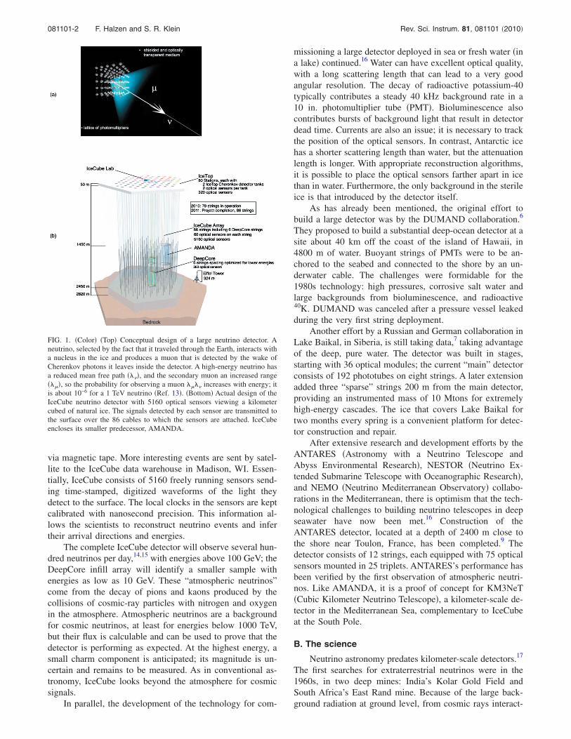
success: neutrino detectors have “seen” the Sun and detecteda supernova in the Large Magellanic Cloud in 1987. Bothobservations were of tremendous importance; the formershowed that neutrinos have a tiny mass, opening the firstcrack in the standard model of particle physics, and the latterconfirmed the theory of stellar evolution as well as the basicnuclear physics of the death of stars. Figure 2 illustrates thecosmic-neutrino energy spectrum covering an enormousrange, from microwave energies �10−12 eV� to 1020 eV.27
The figure is a mixture of observations and theoretical pre-dictions. At low energy, the neutrino sky is dominated byneutrinos produced in the Big Bang. At MeV energy, neutri-nos are produced by supernova explosions; the flux from the1987 event is shown. The figure displays the measuredatmospheric-neutrino flux up to energies of 100 TeV by theAMANDA experiment.26 Atmospheric neutrinos are a key toour story because they are the dominant background for ex-traterrestrial searches. The flux of atmospheric neutrinos fallsdramatically with increasing energy; events above 100 TeVare rare, leaving a clear field of view for extraterrestrialsources.
The highest-energy neutrinos in Fig. 2 are the decayproducts of pions produced by the interactions of cosmicrays with microwave photons.28 Above a threshold of �4�1019 eV, cosmic rays interact with the microwave back-ground, introducing an absorption feature in the cosmic-rayflux, the Greissen–Zatsepin–Kuzmin �GZK� cutoff. As a con-sequence, the mean free path of extragalactic cosmic rayspropagating in the microwave background is limited to
log(Eν /GeV)
dNν/
dEν
[GeV
-1sr
-1s-1
cm-2
]
10-27
10-22
10-17
10-12
10-7
10-2
10 3
10 8
10 13
-15 -10 -5 0 5 10
FIG. 2. �Color online� The cosmic-neutrino spectrum. Sources are the BigBang �C�B�, the Sun, supernovae �SN�, atmospheric neutrinos, active ga-lactic nuclei galaxies, and GZK neutrinos. The data points are from detec-tors at the Frejus underground laboratory �Ref. 21� to the right at the top ofthe figure, and the upper portion of the Atmospheric line at the bottom of thefigure, and from AMANDA �Ref. 26� pp and B at the top and the lower partof the Atmospheric line.
081101-3 F. Halzen and S. R. Klein Rev. Sci. Instrum. 81, 081101 �2010�
roughly 75 Mpc �240�106 light years� and, therefore, thesecondary neutrinos are the only probe of the still-enigmaticsources at longer distances. What they will reveal is a matterof speculation. The calculation of the neutrino flux associ-ated with the observed flux of extragalactic cosmic rays isstraightforward and yields one event per year in a kilometer-scale detector. It is, however, subject to ambiguities, mostnotably from the still-unknown composition of the highest-energy cosmic rays and due to the cosmological evolution ofthe sources.29 The flux, labeled GZK in Fig. 2, shares thehigh-energy neutrino sky with neutrinos from gamma-raybursts and active galactic nuclei.4
In this review, we will first illustrate the origin of theconcept to build a kilometer-scale neutrino detector. It hastaken half a century from the concept to the commissioningof IceCube. It took this long to develop the methodologiesand technologies to build a neutrino telescope; we will de-scribe them next. We complete the article by discussing otherscience covered by this novel instrument.
II. WHY KILOMETER-SCALE DETECTORS?NEUTRINO SOURCES AND COSMIC RAYS
A. Cosmic-ray accelerators and cosmic-beam dumps
Despite a discovery potential touching a wide range ofscientific issues, the construction of IceCube and a futureKM3NeT �Ref. 10� has been largely motivated by the possi-bility of opening a new window on the Universe, using neu-trinos as cosmic messengers. Specifically, we will revisitIceCube’s prospects to detect cosmic neutrinos associatedwith cosmic rays and thus finally reveal their sources.
Cosmic accelerators produce particles with energies inexcess of 108 TeV; we still do not know where or how.30
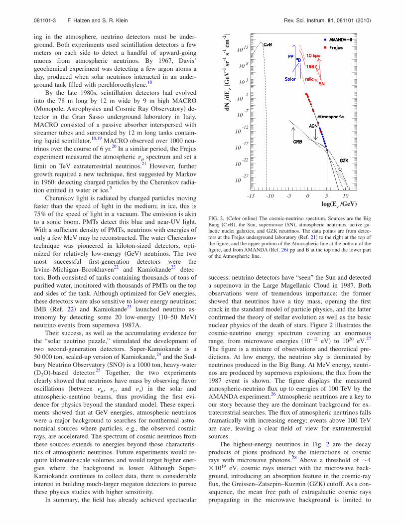
The observed flux of cosmic rays is shown in Fig. 3.27 Theenergy spectrum follows a sequence of three power laws.The first two are separated by a feature dubbed the “knee” atan energy of approximately 3000 TeV. There is evidence thatcosmic rays up to this energy are galactic in origin. Any
association with our galaxy disappears in the vicinity of asecond feature in the spectrum referred to as the “ankle” �seeFig. 3�. Above the ankle, the gyroradius of a proton in thegalactic magnetic field exceeds the size of the galaxy andpoints to the onset of an extragalactic component in the spec-trum that extends to energies beyond 108 TeV. Direct sup-port for this assumption comes from two experiments thathave observed the telltale structure in the cosmic-ray spec-trum resulting from the absorption of the particle flux by themicrowave background, the so-called GZK cutoff. The originof the flux in the intermediate region remains a mystery,although it is routinely assumed that it results from somehigh-energy extension of the reach of galactic accelerators.
Acceleration of protons �or nuclei� to TeV energy andabove likely requires massive bulk flows of relativisticcharged particles. These are likely to originate from excep-tional gravitational forces in the vicinity of black holes orneutron stars. Gravity powers large currents of charged par-ticles that produce high magnetic fields. These fields createthe opportunity for particle acceleration by shocks, similar towhat happens with solar flares. It is a fact that electrons areaccelerated to TeV energy and above near black holes; as-tronomers detect them indirectly by their synchrotron radia-tion. Some must accelerate protons because we observe themas cosmic rays.
How many gamma rays and neutrinos are produced inassociation with the cosmic-ray beam? Generically, acosmic-ray source should also be a “beam dump.” Cosmicrays accelerated in regions of high magnetic fields near blackholes inevitably interact with radiation surrounding them: forinstance, UV photons in active galaxies or MeV photons ingamma-ray-burst fireballs. Neutral and charged pion second-aries are produced by the processes
p + � → � + p and p + � → �+ + n . �1�
Although secondary protons may remain trapped in the highmagnetic fields, neutrons and the pion decay products es-cape. The energy escaping the source is distributed amongcosmic rays, gamma rays, and neutrinos produced by thedecay of neutrons, neutral pions, and charged pions, respec-tively. Kilometer-scale neutrino detectors have the sensitivityto reveal generic cosmic-ray sources with an energy densityin neutrinos comparable to their energy density in cosmicrays and pionic TeV photons.31
In the case of galactic supernova shocks, cosmic raysinteract with gas in the galactic disk, e.g., with dense mo-lecular clouds, producing equal numbers of pions of all threecharges in hadronic collisions p+ p→n ��+�++�−�+X.Here, n is the multiplicity of secondary pions.
This mechanism predicts a relation between cosmic-ray�Np�, gamma-ray �N��, and neutrino �N�� fluxes31
dN�
dE=
1
2�1
8�dN�
dE, �2�
dN�
dE�
nintx�
dNp
dEpEp
x�� . �3�
The first relation reflects the fact that pions decay intogamma rays and neutrinos that carry 1/2 and 1/4 of the en-
log10(Ep/GeV)
Ep2 ·
dNp/
dEp
[GeV
cm-2
s-1sr
-1]
10-9
10-8
10-7
10-6
10-5
10-4
10-3
10-2
10-1
1
2 3 4 5 6 7 8 9 10 11 12
FIG. 3. �Color online� At the energies of interest here, the cosmic-ray spec-trum follows a sequence of three power laws. The first two are separated bythe knee, the second and third by the ankle. Cosmic rays beyond the ankleare a new population of particles produced in extragalactic sources�Ref. 27�.
081101-4 F. Halzen and S. R. Klein Rev. Sci. Instrum. 81, 081101 �2010�
ergy of the parent. This assumes that the four leptons in thedecay �+→��+ �e+ �̄e+��� equally share the charged pion’senergy. N��=N��
=N�e=N��
� is the sum of the neutrino andantineutrino fluxes that are not distinguished by the experi-ments. Oscillations over cosmic baselines yield approxi-mately equal fluxes for the three flavors. The two factorsapply to the hadronic and photoproduction of pions in thesource, respectively. Although this relation only depends onstraightforward particle physics, the second relation of theneutrino to the actual cosmic-ray flux depends on nint, thenumber of interactions determined by the optical depth of thesource for p� interactions. The factor
x� =E�
Ep=
1
4�xp→�
1
20�4�
is the relative energy of the neutrino to the pion. The pioncarries, on average, a fraction xp→��0.2 of the parent protonenergy and shares it roughly equally between the fourleptons.
These relations form the basis for testing the assumptionthat cosmic rays are accelerated in a cosmic source. For amore detailed discussion of these relations, we refer thereader to Ref. 31.
This discussion does not apply to sources that primarilyaccelerate electrons, which do not produce neutrinos. Somecosmic electron accelerators have been identified via theiremission of polarized synchrotron radiation. However, un-ambiguously identifying a source that does not emit synchro-tron radiation is challenging, and unambiguous observationof a cosmic-ray accelerator may require the observation ofneutrinos.
B. Galactic sources
Supernova remnants were proposed as the source of ga-lactic cosmic rays as early as 1934 by Baade and Zwicky;32
their proposal is still a matter of debate. Galactic cosmic raysreach energies of at least several thousand TeV, the knee inthe spectrum. Their interactions with galactic hydrogen inthe vicinity of the accelerator should generate gamma raysfrom the decay of secondary pions that reach energies ofhundreds of TeV. Such sources should be identifiable by arelatively flat energy spectrum that extends to high energywithout attenuation; they have been dubbed PeVatrons.Straightforward energetics arguments show that present airCherenkov telescopes should have the sensitivity necessaryto detect TeV photons from PeVatrons.
They may have been revealed by an all-sky survey in�10 TeV gamma rays with the Milagro detector.33 Sourcesare identified in nearby star-forming regions in Cygnus andin the vicinity of galactic latitude l=40°; some are notreadily associated with known supernova remnants or withnonthermal sources observed at other wavelengths. In fact,some Milagro sources may actually be molecular clouds il-luminated by the cosmic-ray beam accelerated in young rem-nants located within �100 pc. One expects indeed that thehighest-energy cosmic rays are accelerated over a short timeperiod, of the order of 1–10 000 yr when the shock velocityis high. The high-energy particles can produce photons andneutrinos over much longer periods when they diffuse
through the interstellar medium to interact with nearby mo-lecular clouds.34 Star-forming regions provide all ingredientsfor the efficient production of neutrinos: supernovae to ac-celerate cosmic rays and a high density ambient medium,including molecular clouds, as an efficient target for produc-ing pions.
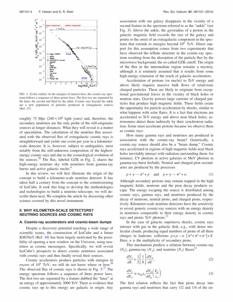
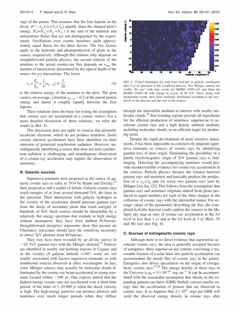
Despite the rapid development of more sensitive instru-ments, it has been impossible to conclusively pinpoint super-nova remnants as sources of cosmic rays by identifyinggamma rays of pion origin. Eliminating the possibility of apurely electromagnetic origin of TeV gamma rays is chal-lenging. Detecting the accompanying neutrinos would pro-vide incontrovertible evidence for cosmic-ray acceleration inthe sources. Particle physics dictates the relation betweengamma rays and neutrinos and basically predicts the produc-tion of a ��+ �̄� pair for every two gamma rays seen byMilagro �see Eq. �2��. This follows from the assumptions thatgamma rays and neutrinos originate indeed from pions pro-duced in equal numbers for each of the three charges in thecollisions of cosmic rays with the interstellar matter. For av-erage values of the parameters describing the flux, the com-pleted IceCube detector could confirm the sources in the Mi-lagro sky map as sites of cosmic-ray acceleration at the 3level in less than 1 yr and at the 5 level in 3 yr �Refs. 35and 36� �see also Fig. 4�.
C. Sources of extragalactic cosmic rays
Although there is no direct evidence that supernovae ac-celerate cosmic rays, the idea is generally accepted becauseof energetics: three supernovae per century converting a rea-sonable fraction of a solar mass into particle acceleration canaccommodate the steady flux of cosmic rays in the galaxy.Energetics also drives speculation on the origin of extraga-lactic cosmic rays.37,38 The energy density of these rays inthe Universe is �E�3�10−19 erg cm−3. It can be accommo-dated with the reasonable assumption that shocks in the ex-panding gamma-ray-burst �GRB� fireball convert similar en-ergy into the acceleration of protons that are observed ascosmic rays. It so happens that 2�1051 ergs per GRB willyield the observed energy density in cosmic rays after
FIG. 4. �Color� Simulated sky map from IceCube in galactic coordinatesafter 5 yr of operation of the completed detector. Two Milagro sources arevisible “by eye” with four events for MGRO J1852+01 and three forMGRO J1908+06 with energy in excess of 40 TeV. These, along withbackground events, have been randomly distributed according to the reso-lution of the detector and the size of the sources.
081101-5 F. Halzen and S. R. Klein Rev. Sci. Instrum. 81, 081101 �2010�
1010 yr, given that their rate is 300 Gpc−3 yr−1. Therefore,300 GRBs per year over Hubble time produce the observedcosmic-ray energy density in the Universe, just as three su-pernovae per century accommodate the steady flux of cosmicrays in the galaxy.31,32
Cosmic rays and synchrotron photons coexist in the ex-panding GRB fireball prior to it reaching transparency andproducing the observed GRB display. Their interactions pro-duce charged pions and neutrinos with a flux that can beestimated from the observed extragalactic cosmic-ray flux�see Eq. �3��. Fireball phenomenology predicts that, on aver-age, nint�1.
Problem solved? Not really: the energy density of ex-tragalactic cosmic rays can also be accommodated by activegalactic nuclei, provided each converts 2�1044 ergs s−1 intoparticle acceleration. As with GRBs, this is an amount thatmatches their output in electromagnetic radiation.39
Waxman and Bahcall40 argued that it is implausible thatthe neutrino flux should exceed the cosmic-ray flux
E�2 dN
dE�
= 5 � 10−11 TeV cm−2 s−1 sr−1. �5�
For the specific example of GRB, we have to scale it down-ward by a factor x��1 /20 �see Eq. �3��. After 7 years ofoperation, AMANDA’s sensitivity is approaching the inter-esting range, but it takes IceCube to explore it.
If GRBs are the sources,41 and the flux is near this limit,then IceCube’s mission is relatively straightforward becausewe expect to observe of the order of 10 �neutrinos /km2� yr−1
in coincidence with GRBs observed by the Swift and Fermisatellites, which translates to a 5 observation.42 Similar sta-tistical power can be obtained by detecting showers pro-duced by �e and ��.
In summary, while the road to identification of sourcesof the galactic cosmic ray has been mapped, the origin of theextragalactic component remains unresolved. Hopefully,neutrinos will reveal the sources.
III. NEUTRINO TELESCOPES: THE CONCEPT
Because of the small neutrino cross sections, a very largedetector is required to observe astrophysical neutrinos. At thesame time, flavor identification is also very desirable sincethe background from atmospheric neutrinos is much lowerfor �e and �� than that for ��. Of course, angular resolution isalso very important for detecting point sources, and energyresolution is important in determining neutrino energy spec-tra, which is important for identifying a diffuse flux of ex-traterrestrial neutrinos.
IceCube detects neutrinos by observing the Cherenkovradiation from the charged particles produced by neutrinointeractions. Charge-current interactions produce a lepton,which carries an average of 50% �for E��10 GeV� to 80%�at high energies� of the neutrino energy; the remainder of
the energy is transferred to the nuclear target. The latter isreleased in the form of a hadronic shower; both the producedlepton and the hadronic shower produce Cherenkov radia-tion. In neutral-current interactions, the neutrino transfers afraction of its energy to a nuclear target, producing just ahadronic shower.
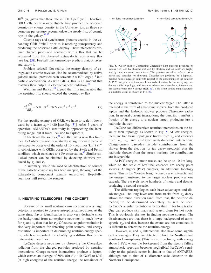
IceCube can differentiate neutrino interactions on the ba-sis of their topology, as shown in Fig. 5. At low energies,there are two basic topologies: tracks from �� and cascadesfrom �e, ��, and all-flavor neutral-current interactions.Charge-current cascades include contributions from theshower from the electron �or tau decay products� plus thehadronic shower from the struck nucleus; the contributionsare inseparable.
At PeV energies, muon tracks can be up to 10 km long,while on the scale of IceCube, cascades are nearly pointsources. At higher �PeV� energies, an additional topologyarises. This is the “double bang” whereby a �� interacts, andthe energy transferred to the target nucleus produces onecascade. The � travels some hundreds of meters and decays,producing a second cascade.
The different topologies each have advantages and dis-advantages. The long lever arm from tracks from �� decayallows the muon direction �and, from that, the neutrino di-rection� to be determined accurately; as will be seen,IceCube’s angular resolution is better than 1° for long tracks.One can produce sky maps and search them for hot spots.This is obviously the key in finding neutrino sources. Thedisadvantages are that there is a large background of atmo-spheric ��, and that, because the events are not contained, itis difficult to determine the neutrino energy.
However, �e and �� interactions also have some signifi-cant advantages. They are detected in both the Northern andSouthern Hemispheres. �This is also true for �� with energyabove 1 PeV, where the background from the steeply fallingatmospheric spectrum becomes negligible.� IceCube’s sensi-tivity to the galactic center is similar to that of ANTARES,although not to that of a kilometer-scale detector in theNorthern Hemisphere.
~ km-long muon tracks from νμ ~ 10m-long cascades from νθ , ντ
17 m}μ
νμ
νθ
с
FIG. 5. �Color online� Contrasting Cherenkov light patterns produced bymuons �left� and by showers initiated by electron and tau neutrinos �right�and by neutral-current interactions. The patterns are often referred to astracks and cascades �or showers�. Cascades are produced by a �approxi-mately� point source of light with respect to the dimensions of the detector.At PeV energies, � leptons travel hundreds of meters before decaying, pro-ducing a third topology, with two cascades—one when the �� interacts andthe second when the � decays �Ref. 43�. This is the double bang signature;a simulated event is shown in Fig. 22.
081101-6 F. Halzen and S. R. Klein Rev. Sci. Instrum. 81, 081101 �2010�
The background of atmospheric �e is significantly lowerand there are almost no atmospheric ��. At higher energies,muons from � decay, the source of atmospheric �e, no longerdecay and the relatively rare K-decays become the dominantsource of background �e.
The neutrino energy may be more precisely determined.Since the events are contained, the energy measurement islargely calorimetric because the light output scales nearlylinearly with the cascade energy. Their energy measurementis superior. One can use energy spectra to differentiate be-tween atmospheric and extraterrestrial neutrinos; the latterhas a harder spectrum.
Tau neutrinos ���� are not absorbed by the Earth.44 In-stead, �� interacting in the Earth produce secondary �� oflower energy, either directly in a neutral-current interactionor via the decay of a tau lepton produced in a charged-current interaction. High-energy �� will thus cascade down tohundreds of TeV energy where the Earth is transparent. Inother words, they are detected with a reduced energy, but arenot absorbed.
Although cascades are nearly pointlike, they are not iso-tropic; light is preferentially emitted at the Cherenkov angle,about 41° in ice. Although this light is heavily scattered be-fore reaching the optical sensors, at energies above 100 TeV,enough directional information may remain to determine theneutrino direction to about 30° �see Ref. 45�. The light pro-duced by cascades spreads over a large volume; in IceCube,a 10 TeV cascade is visible within a radius of about 130 mrising to 460 m at 10 EeV, i.e., the shower radius grows byjust over 50 m/decade in energy.
At energies above 1 PeV in ice, electrons and photonscan interact with multiple atoms, and the Landau–Pomeranchuk–Migdal effect reduces the cross sections forbremsstrahlung and pair production. At energies above100 PeV, electromagnetic showers begin to elongate, reach-ing a length of about 80 m at 100 EeV.46 At these energies,the shower direction might be better determined. At energiesabove 100 PeV, photonuclear interactions must be consid-ered, and even electromagnetic showers will have a hadroniccomponent including some muon production.
The detection of neutrinos of all flavors is important inseparating diffuse extraterrestrial neutrinos from atmosphericneutrinos. Generic cosmic accelerators produce neutrinosfrom the decay of pions with admixture �e :�� :��=1:2 :0.Over cosmic baselines, neutrino oscillations alter the ratio to1:1:1 because approximately one-half of the �� converts into��. The same production ratio is expected for lower energy�below 10 GeV� atmospheric neutrinos, where the muons candecay before interacting. However, at higher energies, themuons interact, and atmospheric neutrinos are largely ��.The flavor ratio depends on the distance the neutrinos havetraveled; extraterrestrial neutrinos should have comparablefluxes of �e, ��, and ��. For in-depth discussion of neutrinodetection, energy measurement, and flavor separation, andfor detailed references, see the IceCube preliminary designdocument11 and Ref. 13.
A. Detection probabilities
To a first approximation, neutrinos are detected whenthey interact inside the instrumented volume. The path lengthL��� traversed within the detector volume by a neutrino withzenith angle � is determined by the detector’s geometry. To afirst approximation, neutrinos are detected if they interactwithin the detector volume, i.e., within the instrumented dis-tance L���. That probability is
P�E�� = 1 − exp�−L
� �E��� L
� �E��, �6�
where
���E�� = ��iceNA�N�E���−1 �7�
is the mean free path in ice for a neutrino of energy E�. Here,�ice=0.9 g cm−3 is the density of the ice, NA=6.022�1023
is Avogadro’s number, and �N�E�� is the neutrino-nucleon cross section. A neutrino flux, dN /dE�
�neutrinos GeV−1 cm−2 s−1�, crossing a detector with energythreshold E�
th and cross-sectional area A�E��� facing the in-cident beam will produce
Nev = T�E�
thA�E��P�E��
dN
dE�
dE� �8�
events after a time T. One must additionally account for thefact that neutrinos may not reach the detector because theyare absorbed in the Earth when they travel along a chord oflength X ��� at zenith angle �. This absorption factor dependson neutrino flavor and must also be included in the probabil-ity P�E�� that the neutrino is detected. Event-rate calcula-tions are discussed in more detail in the appendix of Ref. 36.
So far, the formalism applies to contained events, i.e., weassumed that the neutrino interacted within the instrumenteddistance L���. Furthermore, the “effective” detector areaA�E��� is clearly also a function of zenith angle �. It is notstrictly equal to the geometric cross section of the instru-mented volume facing the incoming neutrino because evenneutrinos interacting outside the instrumented volume mayproduce enough light inside the detector to be detected. Inpractice, A�E��� is determined as a function of the incidentneutrino direction and zenith angle by a full-detector simu-lation including the trigger. It is of the order of 1 km2 forIceCube. Often the neutrino effective area is introduced asA�=AP. Note that the quantity P is calculated rather thanmeasured and is different for muon and tau flavors; we gen-eralize it next.
For muon neutrinos, any neutrino producing a secondarymuon that reaches the detector �and has sufficient energy totrigger it� will be detected �see Fig. 1�a��. Because the muontravels kilometers at TeV energy and tens of kilometers atPeV energy, neutrinos can be detected outside the instru-mented volume; the probability is obtained by substitution inEq. �6�,
L → ��, �9�
therefore,
081101-7 F. Halzen and S. R. Klein Rev. Sci. Instrum. 81, 081101 �2010�
P =��
��
. �10�
Here, �� is the range of the muon determined by its energyloss.
A tau neutrino can be observed provided the tau lepton itproduces reaches the instrumented volume within its life-time. In Eq. �6�, L is replaced by
L → �c� = �E/m�c� , �11�
where m, �, and E are the mass, lifetime, and energy of thetau, respectively. The tau decay length ��=�c��50 m� �E /106 GeV� grows linearly with energy and exceeds therange of the muon near 1018 eV. At even higher energies, thetau eventually ranges out by catastrophic interactions, justlike the muon, despite the reduction of the cross sections bya factor �m� /m��2. The taus trigger the detector but the tracksand �or� showers they produce are mostly indistinguishablefrom those initiated by muon and electron neutrinos �see alsoFig. 5�.
To be clearly recognizable as ��, both the initial neutrinointeraction and the subsequent tau decay must be containedwithin the detector; for a cubic-kilometer detector, this hap-pens for neutrinos with energies from a few PeV to a fewtens of PeV. It might be possible to identify �� that onlyinteract in the detector, or � that decay in the detector,47 butthis has not yet been proven.
B. Muon energy measurement
Muons from �� have ranges from kilometers at TeV en-ergy to tens of kilometers at EeV energy, generating showersalong their track by bremsstrahlung, pair production, andphotonuclear interactions. These are the sources of additionalCherenkov radiation. Because the energy of the muon de-grades along its track, the energy of secondary showers alsogradually diminishes, and the distance from the track overwhich the associated Cherenkov light can trigger a PMT isgradually reduced. The geometry of the light pool surround-ing the muon track is therefore a kilometer-long cone with agradually decreasing radius. At lower energies, of hundredsof GeV and less, the muon becomes minimum-ionizing.
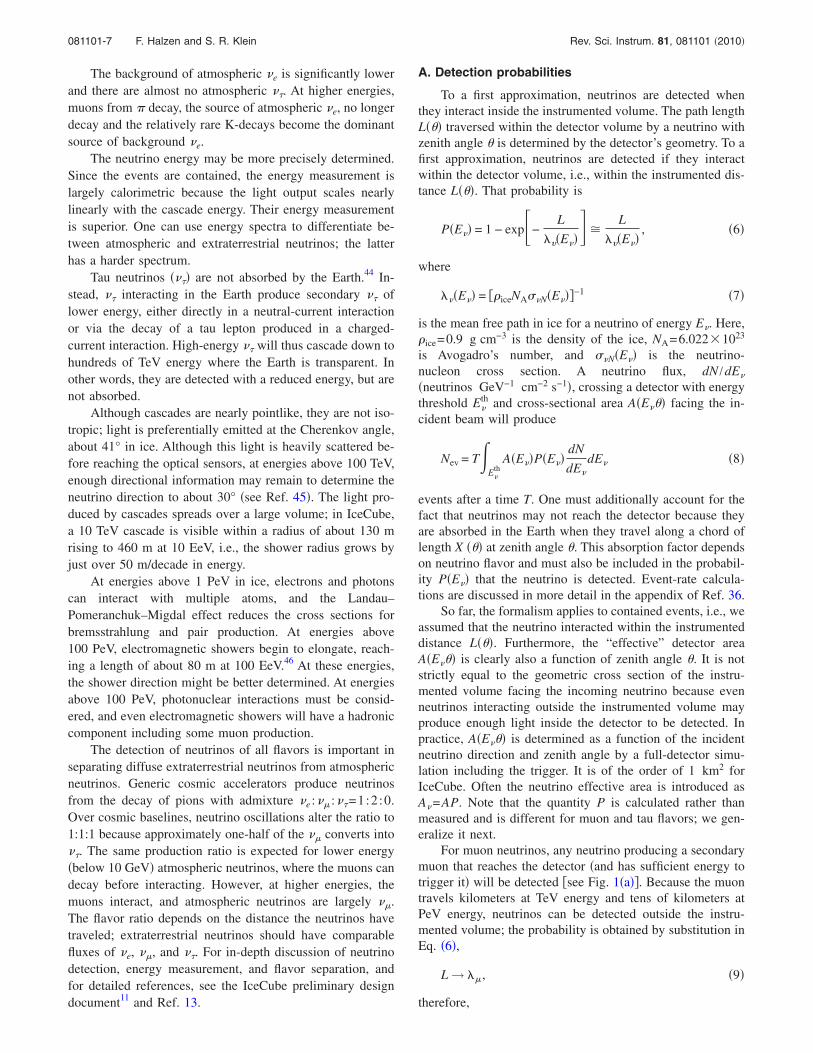
In its first kilometer, a high-energy muon typically losesenergy in a couple of showers of one-tenth of its initial en-ergy. So the initial radius of the cone is the radius of ashower with 10% of the muon energy, e.g., 130 m for a100 TeV muon. Near the end of its range, the muon becomesminimum-ionizing, visible up to about 15 m from the PMT.Figure 6 shows the detection distance as a function of thephotoelectron threshold.
Because of the stochastic nature of the muon’s energyloss, the relationship between the observed �via Cherenkovlight� energy loss and the muon energy varies from muon tomuon. The muon energy in the detector can be determined toroughly a factor of 2. Beyond that, one does not know howfar the muon traveled �and how much energy it lost� beforeentering the detector; an unfolding process is required to de-termine the neutrino energy based on the observed muonenergies.
IV. FROM AMANDA TO ICECUBE: NATURALANTARCTIC ICE AS A CHERENKOV DETECTOR
Neutrino detection in ice was pioneered by theAMANDA collaboration in the late 1990s.48 It requires athick ice sheet, so AMANDA was built in the 2800-m-thickicecap at the Amundsen–Scott South Pole Station. The col-laboration drilled holes in the ice using a hot-water drill andlowered strings of optical sensors before the water in the holerefroze. The station provided everything from a skiway forthe LC-130 turboprops that carried every piece of equipment,plus all of the fuel, to radio and internet communication, andto food and housing for the summer construction crew andthe two or three winter-over scientists who kept AMANDArunning in the winter.
Despite the logistical difficulties, the collaboration low-ered 80 photomultipliers in pressure vessels into a kilometer-deep hole during the 1993–1994 season �Austral summer�.Although most of the sensors survived the unexpectedly highpressures produced as the water in the hole froze, cosmic-raymuon tracks could not be seen. The problem was50-�m-diameter air bubbles trapped in the ice, even at 1 kmdepth. These bubbles limited the light scattering length toless than 50 cm.
Fortunately, it was predicted that near a depth of 1400 m,high pressure would cause the bubbles to collapse. Data con-firmed this, and blue light was measured to have an incred-ibly long absorption length of more than 200 m, reflectingthe purity of the ice. With this understood, four strings ofdetectors were deployed at depths between 1500 and 2000 min the 1995–1996 season.
The next challenge was to separate a single upward-going muon from the roughly 1�106 downward-goingmuons from cosmic-ray air showers. Algorithms with therequired rejection power were developed for this, and neu-trino events were identified. By 2000, the AMANDA detec-tor was complete, with 19 strings and 677 optical sensors. Alater upgrade replaced the time-to-digital conversion/amplitude-to-digital converters �TDC/ADC� electronics with
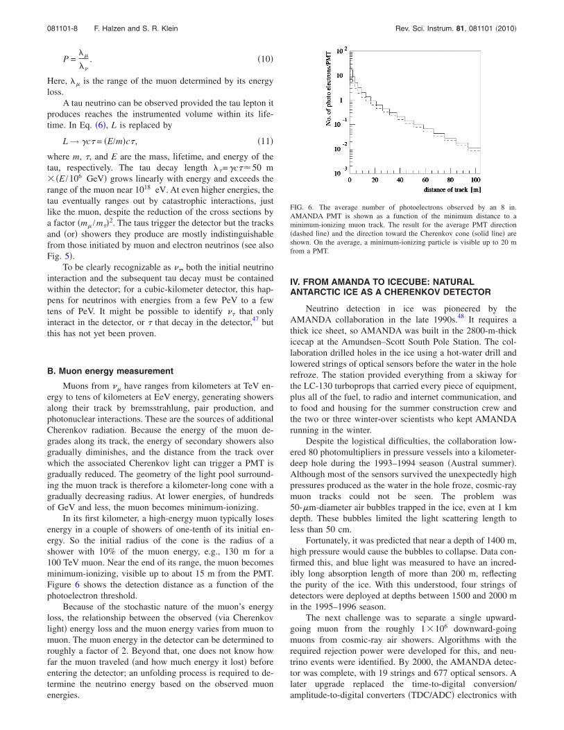
FIG. 6. The average number of photoelectrons observed by an 8 in.AMANDA PMT is shown as a function of the minimum distance to aminimum-ionizing muon track. The result for the average PMT direction�dashed line� and the direction toward the Cherenkov cone �solid line� areshown. On the average, a minimum-ionizing particle is visible up to 20 mfrom a PMT.
081101-8 F. Halzen and S. R. Klein Rev. Sci. Instrum. 81, 081101 �2010�
waveform digitizers. Since 2000, AMANDA-II has been re-cording about 1000 neutrino events per year. For the past fewyears, it operated in coincidence with IceCube.
Despite this success, AMANDA’s limitations were be-coming obvious. It was too small, and it required manpower-intensive annual calibrations. The AMANDA optical mod-ules �OMs� contained 8 in. photomultiplier tubes and littleelse; analog PMT signals were transmitted to the surface.
Although several different approaches were tried overthe years, the analog transmission of signals to the surfacedegraded the resolution. Initially, AMANDA used coaxialcables and then twisted pairs, which transmitted high voltagefor the PMT downward and PMT signals upward. The up-to-2500-m cables stretched the nanosecond PMT rise time tomicroseconds at the surface. Although careful signal process-ing could provide adequate �5–7 ns� first-hit time resolution,there was no possibility to observe multiple hits. The longunamplified transmission required the PMTs to be run at avery high gain, near 109; this had deleterious effects on thePMTs, and a few of them would occasionally “spark,” emit-ting light in the process. In later strings, the electrical trans-mission was replaced with analog optical transmission; thePMT signal controlled a light-emitting diode �LED� in theoptical module. The fibers had far better time resolution, butsuffered from a very limited dynamic range. The light loss inthe optical couplings was very sensitive to vibration and thepassage of time, so the system required manpower-intensiveannual recalibrations.
These problems precluded scaling AMANDA up in size,and the collaboration began exploring other options. Themost attractive, but technically challenging, option was toincorporate the digitizing electronics in each optical module.As a test, AMANDA string 18 included prototype in-OMdigitizers.49 These digitizers ran in parallel with fiber-opticanalog transmission, allowing for both electronics testingand compatibility with AMANDA. String 18 performed well,and the in-OM digitization was adopted by IceCube.
A. IceCube overview
IceCube shares many characteristics with its predeces-sors. As Fig. 1�b� shows, it is a large, tracking calorimeterthat measures the energy deposition in segmented volumes ofAntarctic ice. Because of its size, IceCube can differentiatebetween electron-, muon-, and tau-neutrino interactions. Ithas very good timing resolution, which is used to both accu-rately reconstruct muon trajectories and to find the verticesof contained events. IceCube is a fairly complex experiment;Table I lists and defines some of the IceCube-specific acro-nyms that are used in this review.
When it is completed in 2011, 5160 digital optical mod-ules �DOMs� will instrument 1 km3 of Antarctic ice. Eighty-six vertical strings, each containing 60 DOMs, will be de-ployed in 2500-m-deep holes that were drilled in the ice by ahot-water drill. The water in the hole will refreeze, producing
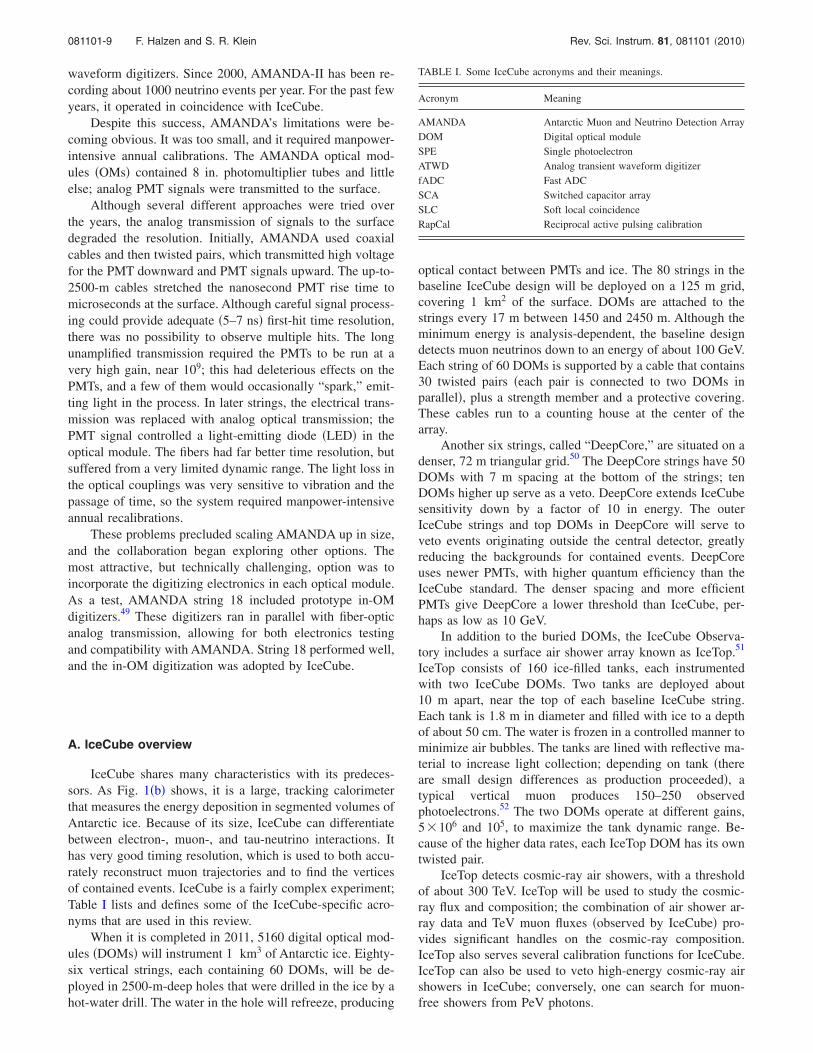
optical contact between PMTs and ice. The 80 strings in thebaseline IceCube design will be deployed on a 125 m grid,covering 1 km2 of the surface. DOMs are attached to thestrings every 17 m between 1450 and 2450 m. Although theminimum energy is analysis-dependent, the baseline designdetects muon neutrinos down to an energy of about 100 GeV.Each string of 60 DOMs is supported by a cable that contains30 twisted pairs �each pair is connected to two DOMs inparallel�, plus a strength member and a protective covering.These cables run to a counting house at the center of thearray.
Another six strings, called “DeepCore,” are situated on adenser, 72 m triangular grid.50 The DeepCore strings have 50DOMs with 7 m spacing at the bottom of the strings; tenDOMs higher up serve as a veto. DeepCore extends IceCubesensitivity down by a factor of 10 in energy. The outerIceCube strings and top DOMs in DeepCore will serve toveto events originating outside the central detector, greatlyreducing the backgrounds for contained events. DeepCoreuses newer PMTs, with higher quantum efficiency than theIceCube standard. The denser spacing and more efficientPMTs give DeepCore a lower threshold than IceCube, per-haps as low as 10 GeV.
In addition to the buried DOMs, the IceCube Observa-tory includes a surface air shower array known as IceTop.51
IceTop consists of 160 ice-filled tanks, each instrumentedwith two IceCube DOMs. Two tanks are deployed about10 m apart, near the top of each baseline IceCube string.Each tank is 1.8 m in diameter and filled with ice to a depthof about 50 cm. The water is frozen in a controlled manner tominimize air bubbles. The tanks are lined with reflective ma-terial to increase light collection; depending on tank �thereare small design differences as production proceeded�, atypical vertical muon produces 150–250 observedphotoelectrons.52 The two DOMs operate at different gains,5�106 and 105, to maximize the tank dynamic range. Be-cause of the higher data rates, each IceTop DOM has its owntwisted pair.
IceTop detects cosmic-ray air showers, with a thresholdof about 300 TeV. IceTop will be used to study the cosmic-ray flux and composition; the combination of air shower ar-ray data and TeV muon fluxes �observed by IceCube� pro-vides significant handles on the cosmic-ray composition.IceTop also serves several calibration functions for IceCube.IceTop can also be used to veto high-energy cosmic-ray airshowers in IceCube; conversely, one can search for muon-free showers from PeV photons.
TABLE I. Some IceCube acronyms and their meanings.
Acronym Meaning
AMANDA Antarctic Muon and Neutrino Detection ArrayDOM Digital optical moduleSPE Single photoelectronATWD Analog transient waveform digitizerfADC Fast ADCSCA Switched capacitor arraySLC Soft local coincidenceRapCal Reciprocal active pulsing calibration
081101-9 F. Halzen and S. R. Klein Rev. Sci. Instrum. 81, 081101 �2010�
IceCube was designed for simple deployment, calibra-tion, and operation. Photomultiplier signals are recorded us-ing fast waveform digitizers in each DOM. Every DOM actsautonomously, receiving power, control, and calibration sig-nals from the surface and returning digital data packets.
IceCube construction began in the 2004–2005 season,with the first string deployment. By January 2010, 79 of thetotal �including DeepCore� strings had been deployed, andthe array should be complete by January 2011.
B. IceCube construction and operations
The construction at the South Pole is difficult, and logis-tics are tough. The construction season is short, from mid-October through mid-February, and being able to drill holesand deploy strings quickly is critical. In order to be able tobuild IceCube in seven seasons, holes had to be drilled inless than 2 days, requiring a power plant of close to 5 MW tomelt ice. Specialized equipment was designed for this effort.
Getting the roughly 1�106 lb of drilling equipment tothe South Pole was another major challenge. The drillingequipment had to be built in modular form, with each com-ponent able to fit into a LC-130 transport plane. Because ofthe high altitude, the plane’s payload is limited, furtherstraining the logistics chain.
IceCube DOMs are deployed in water-filled holes, 61 cmin diameter. The water at the edges of these holes begins torefreeze almost immediately; their 61 cm diameter ensuresthat the holes remain open wide enough to accommodate thecable and DOMs for 30 h; this allows a full string deploy-ment.
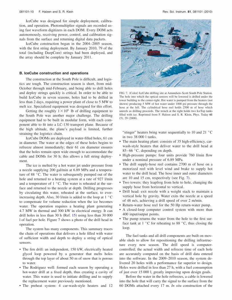
The ice is melted by a hot water jet under pressure froma nozzle supplying 200 gal/min at 6.89 MPa and a tempera-ture of 88 °C. The water is subsequently pumped out of thehole and returned to a heating system at a rate of 927 l/minand a temperature of 1 °C. The water is reheated at the sur-face and returned to the nozzle at depth. Drilling progressesby circulating this water, reheated at the surface, to ever-increasing depth. Also, 30 l/min is added to the loop at 1 °Cto compensate for volume reduction when the ice becomeswater. The operation requires a heating plant generating4.7 MW in thermal and 300 kW in electrical energy. It candrill holes in less than 30 h �Ref. 15� using less than 30 000l of fuel per hole. Figure 7 shows a photo of the drill head inoperation.
The system has many components. This summary tracesthe chain of operations that delivers a hole filled with waterof sufficient width and depth to deploy a string of opticalsensors.
• The firn drill: an independent, 150 kW, electrically heatedglycol loop powered by a generator that melts holesthrough the top layer of about 50 m of snow that is porousto water.
• The Rodriguez well: formed each season by operating ahot-water drill at a fixed depth, thus creating a cavity ofwater. This water is used to initiate drilling and to supplythe replacement water previously mentioned.
• The preheat system: 4 car-wash-style heaters and 12
“stinger” heaters bring water sequentially to 10 and 21 °Cin two 38 000 l tanks.
• The main heating plant: consists of 35 high-efficiency, car-wash-style heaters that deliver water to the drill head at85–66 °C, depending on depth.
• High-pressure pumps: four units provide 760 l/min flowunder a nominal pressure of 6.89 MPa.
• The drill supply-hose reel contains 2700 m of hose on amotorized reel with level wind and brake to supply hotwater to the drill head. The hose inner and outer diametersare 10 and 15 cm, respectively �see Fig. 7�.
• Two towers: they leapfrog from hole to hole, changing thesupply hose from horizontal to vertical.
• Drill head: exit nozzle with a weight stack to maintain avertical hole by gravity. Water exits the nozzle at a speedof 48 m/s, achieving a drill speed of over 2 m/min.
• Return-water hose reel for the 50 Hp return-water pump.• A closed-loop computer control system with more than
400 input/output points.• The pump returns the water from the hole to the first sur-
face tank at 1 °C for reheating to 88 °C, thus closing theloop.
The fuel tanks and all drill components are built on mov-able sleds to allow for repositioning the drilling infrastruc-ture every new season. The drill speed is computer-controlled; the actual width and refreeze time of each holeare accurately computed on the basis of drill data enteredinto the software. In the 2009–2010 season, the system de-livered 20 holes with a performance far superior to design.Holes were drilled in less than 27 h, with a fuel consumptionof just over 15 000 l, greatly improving upon design goals.
Before the water in the hole refreezes, a cable is loweredinto the hole that will carry the signal to the surface from the60 DOMs attached every 17 m. In situ construction of the
FIG. 7. �Color� IceCube drilling site at Amundsen–Scott South Pole Station.The hole into which the optical sensors will be lowered is drilled under thetower building to the center-right. Hot water is pumped from the heaters �notshown� producing 5 MW of hot water under 1000 psi pressure through thehose at the left. The cylindrical hose reel holds 2500 m of hose whichunreels as drilling proceeds. The trench at the right holds two IceTop tanksfilled with ice. Reprinted from F. Halzen and S. R. Klein, Phys. Today 61�5�, 29 �2008�.
081101-10 F. Halzen and S. R. Klein Rev. Sci. Instrum. 81, 081101 �2010�
string and lowering it to depth takes roughly 10 h. Eachstring takes data as soon as the hole refreezes.
C. The ice in IceCube
The ice surrounding the DOMs serves as a Cherenkovradiator. Optical absorption and scattering of the radiatedphotons are both important in determining what IceCube ob-serves. The optical transmission depends strongly on impu-rities in the ice. These impurities were introduced when theice was first laid down as snow. This happens in layers; eachyear snowfall produced a thin, nearly horizontal layer. Forthe ice in IceCube, this happened over roughly the last100 000 yr. Variations in the long term dust level in the at-mosphere during this period, as well as the occasional vol-canic eruption, lead to depth-dependent variations in the ab-sorption and scattering lengths.
Because the bulk of the scattering is in the forward re-gion, light scattering in ice is usually parametrized in termsof the effective scattering length,
�eff =�scat
1 − �cos��� , �11��
where � is the mean scattering angle per scatter. �eff is, ofcourse, frequency-dependent.
Much effort has gone into measuring the optical proper-ties of the ice using artificial light sources and in situ mea-surements. In AMANDA and IceCube, studies have beendone using LEDs and lasers that emit at a variety of wave-lengths. The AMANDA data are still valuable because theyinvolve measurements at many wavelengths. By measuringthe arrival time distributions of photons at different distancesfrom a light source, it is possible to measure both the attenu-ation length and scattering length of the light. These mea-surements, although useful, suffer from a limited resolutionin depth.53
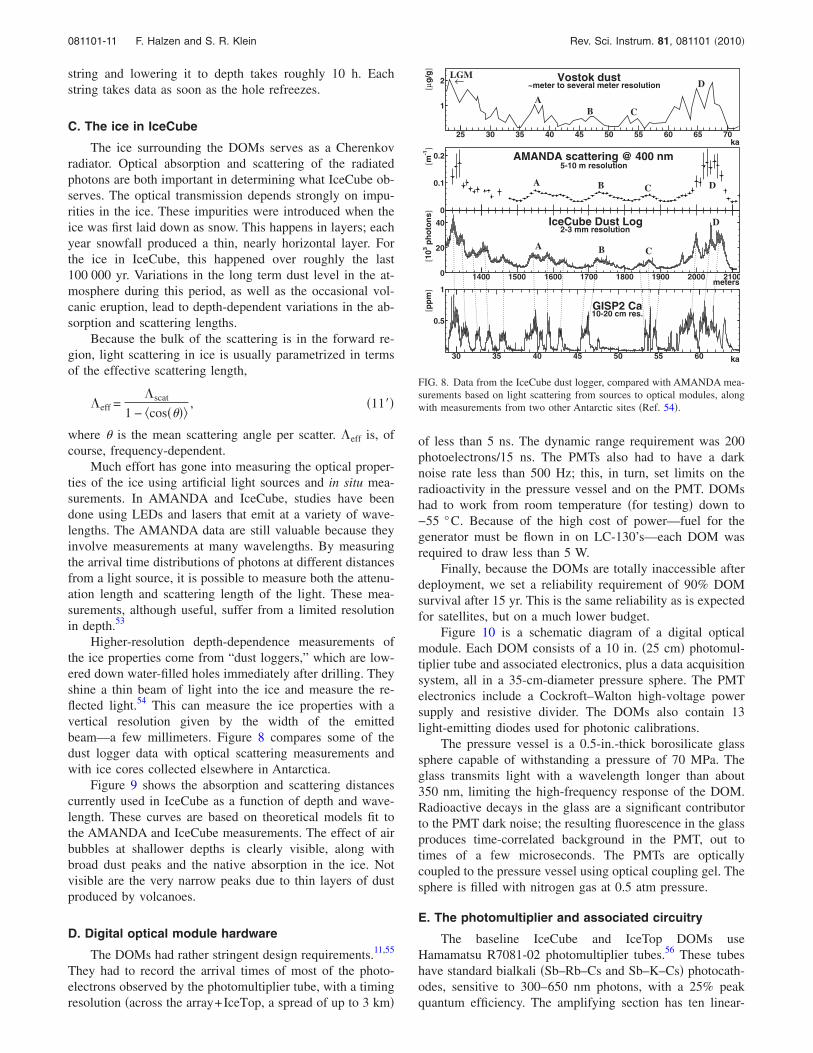
Higher-resolution depth-dependence measurements ofthe ice properties come from “dust loggers,” which are low-ered down water-filled holes immediately after drilling. Theyshine a thin beam of light into the ice and measure the re-flected light.54 This can measure the ice properties with avertical resolution given by the width of the emittedbeam—a few millimeters. Figure 8 compares some of thedust logger data with optical scattering measurements andwith ice cores collected elsewhere in Antarctica.
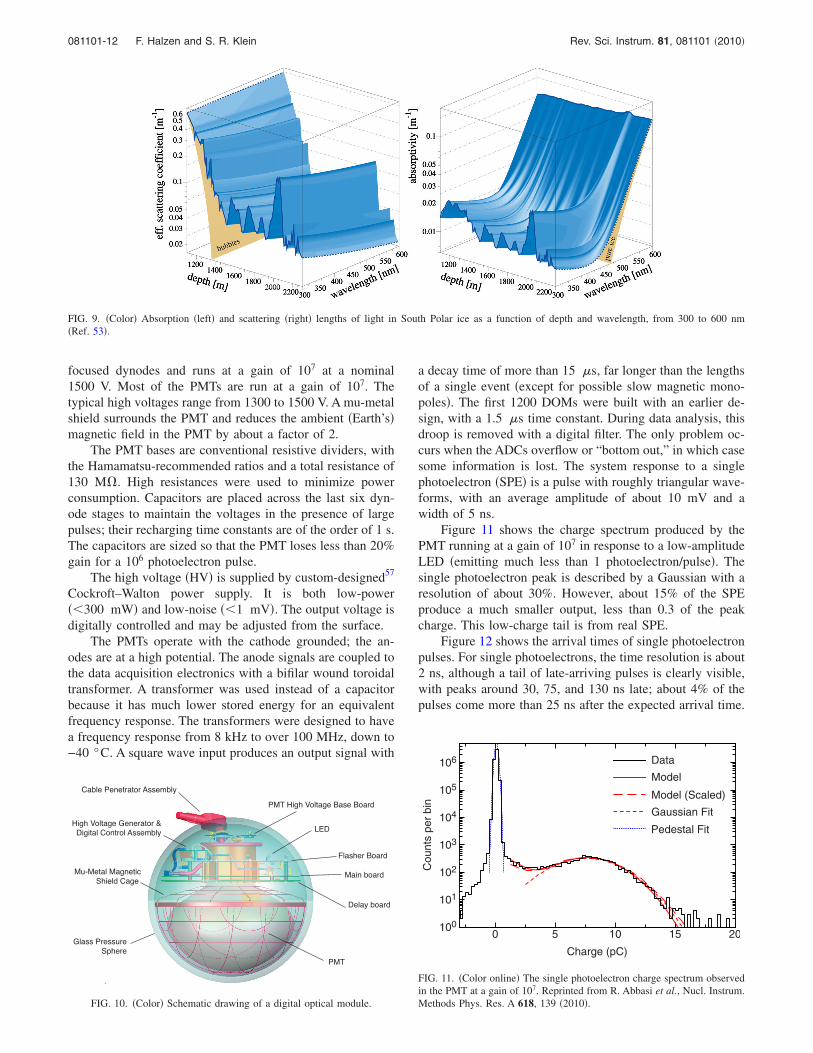
Figure 9 shows the absorption and scattering distancescurrently used in IceCube as a function of depth and wave-length. These curves are based on theoretical models fit tothe AMANDA and IceCube measurements. The effect of airbubbles at shallower depths is clearly visible, along withbroad dust peaks and the native absorption in the ice. Notvisible are the very narrow peaks due to thin layers of dustproduced by volcanoes.
D. Digital optical module hardware
The DOMs had rather stringent design requirements.11,55
They had to record the arrival times of most of the photo-electrons observed by the photomultiplier tube, with a timingresolution �across the array+IceTop, a spread of up to 3 km�
of less than 5 ns. The dynamic range requirement was 200photoelectrons/15 ns. The PMTs also had to have a darknoise rate less than 500 Hz; this, in turn, set limits on theradioactivity in the pressure vessel and on the PMT. DOMshad to work from room temperature �for testing� down to−55 °C. Because of the high cost of power—fuel for thegenerator must be flown in on LC-130’s—each DOM wasrequired to draw less than 5 W.
Finally, because the DOMs are totally inaccessible afterdeployment, we set a reliability requirement of 90% DOMsurvival after 15 yr. This is the same reliability as is expectedfor satellites, but on a much lower budget.
Figure 10 is a schematic diagram of a digital opticalmodule. Each DOM consists of a 10 in. �25 cm� photomul-tiplier tube and associated electronics, plus a data acquisitionsystem, all in a 35-cm-diameter pressure sphere. The PMTelectronics include a Cockroft–Walton high-voltage powersupply and resistive divider. The DOMs also contain 13light-emitting diodes used for photonic calibrations.
The pressure vessel is a 0.5-in.-thick borosilicate glasssphere capable of withstanding a pressure of 70 MPa. Theglass transmits light with a wavelength longer than about350 nm, limiting the high-frequency response of the DOM.Radioactive decays in the glass are a significant contributorto the PMT dark noise; the resulting fluorescence in the glassproduces time-correlated background in the PMT, out totimes of a few microseconds. The PMTs are opticallycoupled to the pressure vessel using optical coupling gel. Thesphere is filled with nitrogen gas at 0.5 atm pressure.
E. The photomultiplier and associated circuitry
The baseline IceCube and IceTop DOMs useHamamatsu R7081-02 photomultiplier tubes.56 These tubeshave standard bialkali �Sb–Rb–Cs and Sb–K–Cs� photocath-odes, sensitive to 300–650 nm photons, with a 25% peakquantum efficiency. The amplifying section has ten linear-
1
2
25 30 35 40 45 50 55 60 65 70ka
[μg
/g]
LGM←
AB C
DVostok dust
~meter to several meter resolution
0
0.1
0.2
[m-1
]
A B C D
AMANDA scattering @ 400 nm5-10 m resolution
0
20
40
1400 1500 1600 1700 1800 1900 2000 2100meters
[10
3p
ho
ton
s]
A B C
DIceCube Dust Log2-3 mm resolution
0.5
1
30 35 40 45 50 55 60 ka
[pp
m]
GISP2 Ca10-20 cm res.
FIG. 8. Data from the IceCube dust logger, compared with AMANDA mea-surements based on light scattering from sources to optical modules, alongwith measurements from two other Antarctic sites �Ref. 54�.
081101-11 F. Halzen and S. R. Klein Rev. Sci. Instrum. 81, 081101 �2010�
focused dynodes and runs at a gain of 107 at a nominal1500 V. Most of the PMTs are run at a gain of 107. Thetypical high voltages range from 1300 to 1500 V. A mu-metalshield surrounds the PMT and reduces the ambient �Earth’s�magnetic field in the PMT by about a factor of 2.
The PMT bases are conventional resistive dividers, withthe Hamamatsu-recommended ratios and a total resistance of130 M�. High resistances were used to minimize powerconsumption. Capacitors are placed across the last six dyn-ode stages to maintain the voltages in the presence of largepulses; their recharging time constants are of the order of 1 s.The capacitors are sized so that the PMT loses less than 20%gain for a 106 photoelectron pulse.
The high voltage �HV� is supplied by custom-designed57
Cockroft–Walton power supply. It is both low-power��300 mW� and low-noise ��1 mV�. The output voltage isdigitally controlled and may be adjusted from the surface.
The PMTs operate with the cathode grounded; the an-odes are at a high potential. The anode signals are coupled tothe data acquisition electronics with a bifilar wound toroidaltransformer. A transformer was used instead of a capacitorbecause it has much lower stored energy for an equivalentfrequency response. The transformers were designed to havea frequency response from 8 kHz to over 100 MHz, down to−40 °C. A square wave input produces an output signal with
a decay time of more than 15 �s, far longer than the lengthsof a single event �except for possible slow magnetic mono-poles�. The first 1200 DOMs were built with an earlier de-sign, with a 1.5 �s time constant. During data analysis, thisdroop is removed with a digital filter. The only problem oc-curs when the ADCs overflow or “bottom out,” in which casesome information is lost. The system response to a singlephotoelectron �SPE� is a pulse with roughly triangular wave-forms, with an average amplitude of about 10 mV and awidth of 5 ns.
Figure 11 shows the charge spectrum produced by thePMT running at a gain of 107 in response to a low-amplitudeLED �emitting much less than 1 photoelectron/pulse�. Thesingle photoelectron peak is described by a Gaussian with aresolution of about 30%. However, about 15% of the SPEproduce a much smaller output, less than 0.3 of the peakcharge. This low-charge tail is from real SPE.
Figure 12 shows the arrival times of single photoelectronpulses. For single photoelectrons, the time resolution is about2 ns, although a tail of late-arriving pulses is clearly visible,with peaks around 30, 75, and 130 ns late; about 4% of thepulses come more than 25 ns after the expected arrival time.
FIG. 9. �Color� Absorption �left� and scattering �right� lengths of light in South Polar ice as a function of depth and wavelength, from 300 to 600 nm�Ref. 53�.
Cable Penetrator Assembly
High Voltage Generator &Digital Control Assembly
Mu-Metal MagneticShield Cage
Glass PressureSphere
PMT High Voltage Base Board
LED
Flasher Board
Main board
Delay board
PMT
FIG. 10. �Color� Schematic drawing of a digital optical module.
0 5 10 15 20100
101
102
103
104
105
106
Charge (pC)
Co
un
tsp
er
bin
Pedestal Fit
Gaussian Fit
Model
Model (Scaled)
Data
FIG. 11. �Color online� The single photoelectron charge spectrum observedin the PMT at a gain of 107. Reprinted from R. Abbasi et al., Nucl. Instrum.Methods Phys. Res. A 618, 139 �2010�.
081101-12 F. Halzen and S. R. Klein Rev. Sci. Instrum. 81, 081101 �2010�
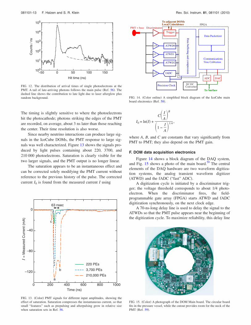
The timing is slightly sensitive to where the photoelectronshit the photocathode; photons striking the edges of the PMTare recorded, on average, about 3 ns later than those reachingthe center. Their time resolution is also worse.
Since nearby neutrino interactions can produce large sig-nals in the IceCube DOMs, the PMT response to large sig-nals was well characterized. Figure 13 shows the signals pro-duced by light pulses containing about 220, 3700, and210 000 photoelectrons. Saturation is clearly visible for thetwo larger signals, and the PMT output is no longer linear.
The saturation appears to be an instantaneous effect andcan be corrected solely modifying the PMT current withoutreference to the previous history of the pulse. The correctedcurrent I0 is found from the measured current I using
I0 = ln�I� +
C I
A�B
1 −I
A�1/4 ,
where A, B, and C are constants that vary significantly fromPMT to PMT; they also depend on the PMT gain.
F. DOM data acquisition electronics
Figure 14 shows a block diagram of the DAQ system,and Fig. 15 shows a photo of the main board.59 The centralelements of the DAQ hardware are two waveform digitiza-tion systems, the analog transient waveform digitizer�ATWD� and the fADC �“fast” ADC�.
A digitization cycle is initiated by a discriminator trig-ger; the voltage threshold corresponds to about 1/4 photo-electron. When the discriminator fires, the field-programmable gate array �FPGA� starts ATWD and fADCdigitization synchronously, on the next clock edge.
A 70-ns-long delay line is used to delay the signal to theATWDs so that the PMT pulse appears near the beginning ofthe digitization cycle. To maximize reliability, this delay line
–50 0 50 100 150100
101
102
103
104
105
Hit time (ns)
Counts
/n
s
FIG. 12. The distribution of arrival times of single photoelectrons at thePMT. A tail of late-arriving photons follows the main pulse �Ref. 56�. Thedashed line shows the contribution to late light due to laser afterglow plusrandom background.
0 200 400 600 800 1000
–120
–80
–40
0
Time (ns)
I=
Measure
dC
urr
ent(m
A)
220 PEs
3,700 PEs
210,000 PEs
63 nsec
a
b
c
FIG. 13. �Color� PMT signals for different input amplitudes, showing theeffect of saturation. Saturation compresses the instantaneous current, so thatsmall “features” such as prepulsing and afterpulsing grow in relative sizewhen saturation sets in Ref. 56.
Data
bu
ffering
and
com
pressio
n
Trigger
PMT + baseFPGA
ATWD1
fADC
ATWD2
x2
x0.25
x23
x16
CommunicationsTime Calibration
Data Packetizer
Precision Clock DC:DCConverter
ADC DAC
Local CoincidenceDiscriminator
To Surface
To adjacent DOMs
ATWD0
FIG. 14. �Color online� A simplified block diagram of the IceCube mainboard electronics �Ref. 58�.
FIG. 15. �Color� A photograph of the DOM Main board. The circular boardfits in the pressure vessel, while the cutout provides room for the neck of thePMT �Ref. 59�.
081101-13 F. Halzen and S. R. Klein Rev. Sci. Instrum. 81, 081101 �2010�
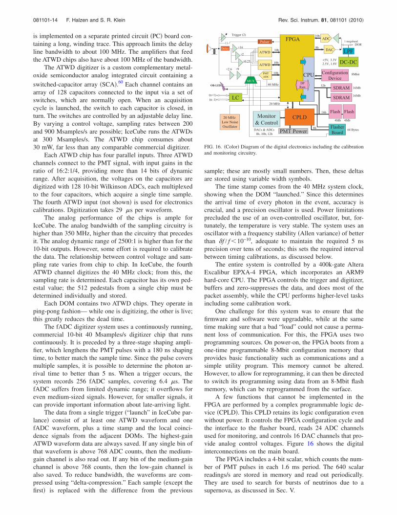
is implemented on a separate printed circuit �PC� board con-taining a long, winding trace. This approach limits the delayline bandwidth to about 100 MHz. The amplifiers that feedthe ATWD chips also have about 100 MHz of the bandwidth.
The ATWD digitizer is a custom complementary metal-oxide semiconductor analog integrated circuit containing a
switched-capacitor array �SCA�.60 Each channel contains anarray of 128 capacitors connected to the input via a set ofswitches, which are normally open. When an acquisitioncycle is launched, the switch to each capacitor is closed, inturn. The switches are controlled by an adjustable delay line.By varying a control voltage, sampling rates between 200and 900 Msamples/s are possible; IceCube runs the ATWDsat 300 Msamples/s. The ATWD chip consumes about30 mW, far less than any comparable commercial digitizer.
Each ATWD chip has four parallel inputs. Three ATWDchannels connect to the PMT signal, with input gains in theratio of 16:2:1/4, providing more than 14 bits of dynamicrange. After acquisition, the voltages on the capacitors aredigitized with 128 10-bit Wilkinson ADCs, each multiplexedto the four capacitors, which acquire a single time sample.The fourth ATWD input �not shown� is used for electronicscalibrations. Digitization takes 29 �s per waveform.
The analog performance of the chips is ample forIceCube. The analog bandwidth of the sampling circuitry ishigher than 350 MHz, higher than the circuitry that precedesit. The analog dynamic range of 2500:1 is higher than for the10-bit outputs. However, some effort is required to calibratethe data. The relationship between control voltage and sam-pling rate varies from chip to chip. In IceCube, the fourthATWD channel digitizes the 40 MHz clock; from this, thesampling rate is determined. Each capacitor has its own ped-estal value; the 512 pedestals from a single chip must bedetermined individually and stored.
Each DOM contains two ATWD chips. They operate inping-pong fashion— while one is digitizing, the other is live;this greatly reduces the dead time.
The fADC digitizer system uses a continuously running,commercial 10-bit 40 Msamples/s digitizer chip that runscontinuously. It is preceded by a three-stage shaping ampli-fier, which lengthens the PMT pulses with a 180 ns shapingtime, to better match the sample time. Since the pulse coversmultiple samples, it is possible to determine the photon ar-rival time to better than 5 ns. When a trigger occurs, thesystem records 256 fADC samples, covering 6.4 �s. ThefADC suffers from limited dynamic range; it overflows foreven medium-sized signals. However, for smaller signals, itcan provide important information about late-arriving light.
The data from a single trigger �“launch” in IceCube par-lance� consist of at least one ATWD waveform and onefADC waveform, plus a time stamp and the local coinci-dence signals from the adjacent DOMs. The highest-gainATWD waveform data are always saved. If any single bin ofthat waveform is above 768 ADC counts, then the medium-gain channel is also read out. If any bin of the medium-gainchannel is above 768 counts, then the low-gain channel isalso saved. To reduce bandwidth, the waveforms are com-pressed using “delta-compression.” Each sample �except thefirst� is replaced with the difference from the previous
sample; these are mostly small numbers. Then, these deltasare stored using variable width symbols.
The time stamp comes from the 40 MHz system clock,showing when the DOM “launched.” Since this determinesthe arrival time of every photon in the event, accuracy iscrucial, and a precision oscillator is used. Power limitationsprecluded the use of an oven-controlled oscillator, but, for-tunately, the temperature is very stable. The system uses anoscillator with a frequency stability �Allen variance� of betterthan �f / f �10−10, adequate to maintain the required 5 nsprecision over tens of seconds; this sets the required intervalbetween timing calibrations, as discussed below.
The entire system is controlled by a 400k-gate AlteraExcalibur EPXA-4 FPGA, which incorporates an ARM9hard-core CPU. The FPGA controls the trigger and digitizer,buffers and zero-suppresses the data, and does most of thepacket assembly, while the CPU performs higher-level tasksincluding some calibration work.
One challenge for this system was to ensure that thefirmware and software were upgradable, while at the sametime making sure that a bad “load” could not cause a perma-nent loss of communication. For this, the FPGA uses twoprogramming sources. On power-on, the FPGA boots from aone-time programmable 8-Mbit configuration memory thatprovides basic functionality such as communications and asimple utility program. This memory cannot be altered.However, to allow for reprogramming, it can then be directedto switch its programming using data from an 8-Mbit flashmemory, which can be reprogrammed from the surface.
A few functions that cannot be implemented in theFPGA are performed by a complex programmable logic de-vice �CPLD�. This CPLD retains its logic configuration evenwithout power. It controls the FPGA configuration cycle andthe interface to the flasher board, reads 24 ADC channelsused for monitoring, and controls 16 DAC channels that pro-vide analog control voltages. Figure 16 shows the digitalinterconnections on the main board.
The FPGA includes a 4-bit scalar, which counts the num-ber of PMT pulses in each 1.6 ms period. The 640 scalarreadings/s are stored in memory and read out periodically.They are used to search for bursts of neutrinos due to asupernova, as discussed in Sec. V.
FPGA
CPU
CPLDFlash Flash
PMT Power
SDRAM
SDRAM
ATWD
ATWD
DAC
Monitor& Control
LPF
LC
×16
×2
×0.25
FlasherBoard
Pulser
DACs & ADCs
4Mb 4Mb
16Mb
16Mb
3.3V2.5V, 1.8V
64 Bytes
Trigger (2)ADC
20 MHzLow NoiseOscillator
20 MHz
40 MHzMUX
(n+1)(n–1)
DOR
OB-LED
×2.6 ×9
10b
10b
10b
10b
8b
32b
16b
8b
8b, 10b, 12b
DPRam
1 megabaud
DC-DC
ConfigurationDevice
8Mbit
Delay
±5V,
PMTADC
FIG. 16. �Color� Diagram of the digital electronics including the calibrationand monitoring circuitry.
081101-14 F. Halzen and S. R. Klein Rev. Sci. Instrum. 81, 081101 �2010�
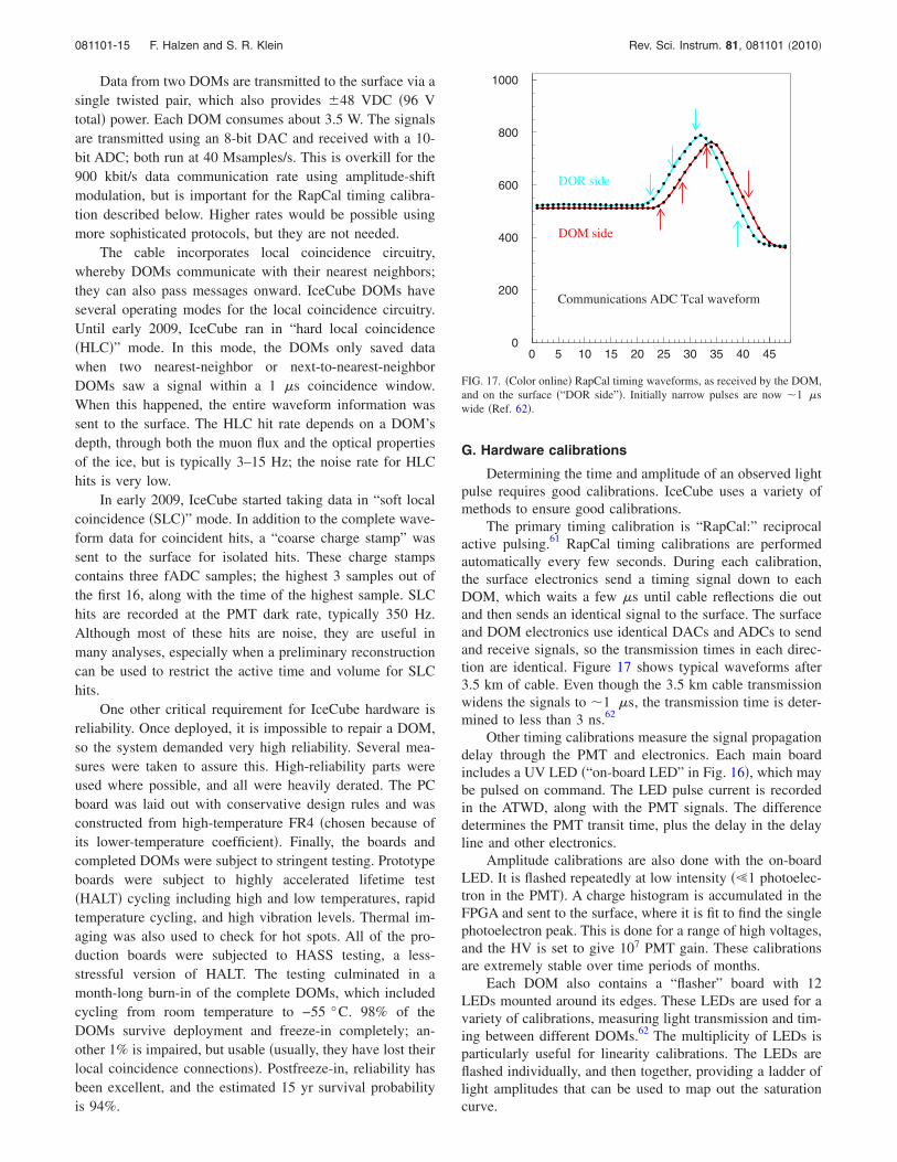
Data from two DOMs are transmitted to the surface via asingle twisted pair, which also provides �48 VDC �96 Vtotal� power. Each DOM consumes about 3.5 W. The signalsare transmitted using an 8-bit DAC and received with a 10-bit ADC; both run at 40 Msamples/s. This is overkill for the900 kbit/s data communication rate using amplitude-shiftmodulation, but is important for the RapCal timing calibra-tion described below. Higher rates would be possible usingmore sophisticated protocols, but they are not needed.
The cable incorporates local coincidence circuitry,whereby DOMs communicate with their nearest neighbors;they can also pass messages onward. IceCube DOMs haveseveral operating modes for the local coincidence circuitry.Until early 2009, IceCube ran in “hard local coincidence�HLC�” mode. In this mode, the DOMs only saved datawhen two nearest-neighbor or next-to-nearest-neighborDOMs saw a signal within a 1 �s coincidence window.When this happened, the entire waveform information wassent to the surface. The HLC hit rate depends on a DOM’sdepth, through both the muon flux and the optical propertiesof the ice, but is typically 3–15 Hz; the noise rate for HLChits is very low.
In early 2009, IceCube started taking data in “soft localcoincidence �SLC�” mode. In addition to the complete wave-form data for coincident hits, a “coarse charge stamp” wassent to the surface for isolated hits. These charge stampscontains three fADC samples; the highest 3 samples out ofthe first 16, along with the time of the highest sample. SLChits are recorded at the PMT dark rate, typically 350 Hz.Although most of these hits are noise, they are useful inmany analyses, especially when a preliminary reconstructioncan be used to restrict the active time and volume for SLChits.
One other critical requirement for IceCube hardware isreliability. Once deployed, it is impossible to repair a DOM,so the system demanded very high reliability. Several mea-sures were taken to assure this. High-reliability parts wereused where possible, and all were heavily derated. The PCboard was laid out with conservative design rules and wasconstructed from high-temperature FR4 �chosen because ofits lower-temperature coefficient�. Finally, the boards andcompleted DOMs were subject to stringent testing. Prototypeboards were subject to highly accelerated lifetime test�HALT� cycling including high and low temperatures, rapidtemperature cycling, and high vibration levels. Thermal im-aging was also used to check for hot spots. All of the pro-duction boards were subjected to HASS testing, a less-stressful version of HALT. The testing culminated in amonth-long burn-in of the complete DOMs, which includedcycling from room temperature to −55 °C. 98% of theDOMs survive deployment and freeze-in completely; an-other 1% is impaired, but usable �usually, they have lost theirlocal coincidence connections�. Postfreeze-in, reliability hasbeen excellent, and the estimated 15 yr survival probabilityis 94%.
G. Hardware calibrations
Determining the time and amplitude of an observed lightpulse requires good calibrations. IceCube uses a variety ofmethods to ensure good calibrations.
The primary timing calibration is “RapCal:” reciprocalactive pulsing.61 RapCal timing calibrations are performedautomatically every few seconds. During each calibration,the surface electronics send a timing signal down to eachDOM, which waits a few �s until cable reflections die outand then sends an identical signal to the surface. The surfaceand DOM electronics use identical DACs and ADCs to sendand receive signals, so the transmission times in each direc-tion are identical. Figure 17 shows typical waveforms after3.5 km of cable. Even though the 3.5 km cable transmissionwidens the signals to �1 �s, the transmission time is deter-mined to less than 3 ns.62
Other timing calibrations measure the signal propagationdelay through the PMT and electronics. Each main boardincludes a UV LED �“on-board LED” in Fig. 16�, which maybe pulsed on command. The LED pulse current is recordedin the ATWD, along with the PMT signals. The differencedetermines the PMT transit time, plus the delay in the delayline and other electronics.
Amplitude calibrations are also done with the on-boardLED. It is flashed repeatedly at low intensity ��1 photoelec-tron in the PMT�. A charge histogram is accumulated in theFPGA and sent to the surface, where it is fit to find the singlephotoelectron peak. This is done for a range of high voltages,and the HV is set to give 107 PMT gain. These calibrationsare extremely stable over time periods of months.
Each DOM also contains a “flasher” board with 12LEDs mounted around its edges. These LEDs are used for avariety of calibrations, measuring light transmission and tim-ing between different DOMs.62 The multiplicity of LEDs isparticularly useful for linearity calibrations. The LEDs areflashed individually, and then together, providing a ladder oflight amplitudes that can be used to map out the saturationcurve.
DOR side
DOM side
Communications ADC Tcal waveform
0
200
400
600
800
1000
0 5 10 15 20 25 30 35 40 45
FIG. 17. �Color online� RapCal timing waveforms, as received by the DOM,and on the surface �“DOR side”�. Initially narrow pulses are now �1 �swide �Ref. 62�.
081101-15 F. Halzen and S. R. Klein Rev. Sci. Instrum. 81, 081101 �2010�
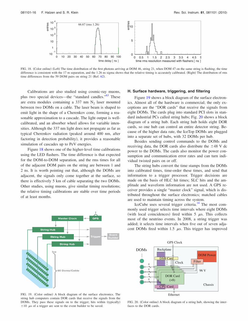
Calibrations are also studied using cosmic-ray muons,plus two special devices—the “standard candles.”63 Theseare extra modules containing a 337 nm N2 laser mountedbetween two DOMs on a cable. The laser beam is shaped toemit light in the shape of a Cherenkov cone, forming a rea-sonable approximation to a cascade. The light output is well-calibrated, and an absorber wheel allows for variable inten-sities. Although the 337 nm light does not propagate as far astypical Cherenkov radiation �peaked around 400 nm, afterfactoring in detection probability�, it provides a reasonablesimulation of cascades up to PeV energies.
Figure 18 shows one of the higher-level time calibrationsusing the LED flashers. The time difference is that expectedfor the DOM-to-DOM separation, and the rms times for allof the adjacent DOM pairs on the string are between 1 and2 ns. It is worth pointing out that, although the DOMs areadjacent, the signals only come together at the surface, sothere is effectively 5 km of cable separating the two DOMs.Other studies, using muons, give similar timing resolutions;the relative timing calibrations are stable over time periodsof at least months.
H. Surface hardware, triggering, and filtering
Figure 19 shows a block diagram of the surface electron-ics. Almost all of the hardware is commercial; the only ex-ceptions are the “DOR cards” that receive the signals fromeight DOMs. The cards plug into standard PCI slots in stan-dard industrial PCs called string hubs; Fig. 20 shows a blockdiagram of a string hub. Each string hub holds eight DORcards, so one hub can control an entire detector string. Be-cause of the higher data rate, the IceTop DOMs are pluggedinto a separate set of hubs, with 32 DOMs per hub.
Besides sending control commands to the DOMs andreceiving data, the DOR cards also distribute the �48 V dcpower to the DOMs. The cards also monitor the power con-sumption and communication error rates and can turn indi-vidual twisted pairs on or off.
The string hubs convert the time stamps from the DOMsinto calibrated times, time-order these times, and send thatinformation to a trigger processor. Trigger decisions aremade on the basis of HLC hit times; SLC hits and the am-plitude and waveform information are not used. A GPS re-ceiver provides a single “master clock” signal, which is dis-tributed throughout the surface electronics; matched cablesare used to maintain timing across the system.
IceCube uses several trigger criteria.14 The most com-monly used trigger selects time intervals where eight DOMs�with local coincidences� fired within 5 �s. This collectsmost of the neutrino events. In 2008, a string trigger wasadded; it selects time intervals when five out of seven adja-cent DOMs fired within 1.5 �s. This trigger has improved
FIG. 19. �Color online� A block diagram of the surface electronics. Thestring hub computers contain DOR cards that receive the signals from theDOMs. They pass these signals on to the trigger; hits within �typically��10 �s of a trigger are sent to the event builder to be saved.
time rms resolution measured with flashers [ ns ]
entries
0
5
10
0 0.5 1 1.5 2 2.5 3 3.5 4 4.5 5
66.67 (rms 1.26)
time delay [ ns ]
entries
10-11
10
10 2
10 3
10 4
0 10 20 30 40 50 60 70 80 90 100
FIG. 18. �Color online� �Left� The time distribution of the first photons arriving at DOM 46, string 21, when DOM 47 on the same string is flashing; the timedifference is consistent with the 17 m separation, and the 1.26 ns sigma shows that the relative timing is accurately calibrated. �Right� The distribution of rmstime differences from the 59 DOM pairs on string 21 �Ref. 62�.
FilterDSB Card
2222
DOMsDOM Power
DOR Cards
Backplane
96 VDOR Card(×8)
Clock
Chassis
GPS Clock
CPU Card
Ethernet
4444
FIG. 20. �Color online� A block diagram of a string hub, showing the inter-faces to the DOR cards.
081101-16 F. Halzen and S. R. Klein Rev. Sci. Instrum. 81, 081101 �2010�
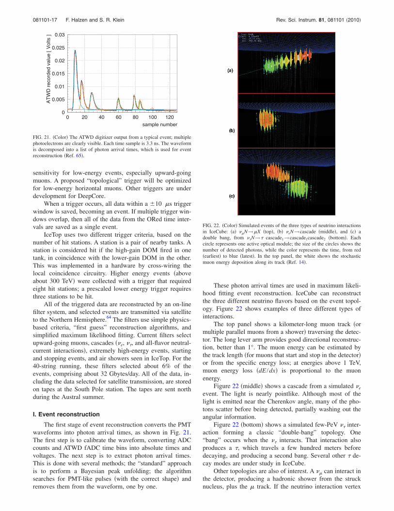
sensitivity for low-energy events, especially upward-goingmuons. A proposed “topological” trigger will be optimizedfor low-energy horizontal muons. Other triggers are underdevelopment for DeepCore.
When a trigger occurs, all data within a �10 �s triggerwindow is saved, becoming an event. If multiple trigger win-dows overlap, then all of the data from the ORed time inter-vals are saved as a single event.
IceTop uses two different trigger criteria, based on thenumber of hit stations. A station is a pair of nearby tanks. Astation is considered hit if the high-gain DOM fired in onetank, in coincidence with the lower-gain DOM in the other.This was implemented in a hardware by cross-wiring thelocal coincidence circuitry. Higher energy events �aboveabout 300 TeV� were collected with a trigger that requiredeight hit stations; a prescaled lower energy trigger requiresthree stations to be hit.
All of the triggered data are reconstructed by an on-linefilter system, and selected events are transmitted via satelliteto the Northern Hemisphere.64 The filters use simple physics-based criteria, “first guess” reconstruction algorithms, andsimplified maximum likelihood fitting. Current filters selectupward-going muons, cascades ��e, ��, and all-flavor neutral-current interactions�, extremely high-energy events, startingand stopping events, and air showers seen in IceTop. For the40-string running, these filters selected about 6% of theevents, comprising about 32 Gbytes/day. All of the data, in-cluding the data selected for satellite transmission, are storedon tapes at the South Pole station. The tapes are sent northduring the Austral summer.
I. Event reconstruction
The first stage of event reconstruction converts the PMTwaveforms into photon arrival times, as shown in Fig. 21.The first step is to calibrate the waveform, converting ADCcounts and ATWD fADC time bins into absolute times andvoltages. The next step is to extract photon arrival times.This is done with several methods; the “standard” approachis to perform a Bayesian peak unfolding; the algorithmsearches for PMT-like pulses �with the correct shape� andremoves them from the waveform, one by one.
These photon arrival times are used in maximum likeli-hood fitting event reconstruction. IceCube can reconstructthe three different neutrino flavors based on the event topol-ogy. Figure 22 shows examples of three different types ofinteractions.
The top panel shows a kilometer-long muon track �ormultiple parallel muons from a shower� traversing the detec-tor. The long lever arm provides good directional reconstruc-tion, better than 1°. The muon energy can be estimated bythe track length �for muons that start and stop in the detector�or from the specific energy loss; at energies above 1 TeV,muon energy loss �dE /dx� is proportional to the muonenergy.
Figure 22 �middle� shows a cascade from a simulated �e
event. The light is nearly pointlike. Although most of thelight is emitted near the Cherenkov angle, many of the pho-tons scatter before being detected, partially washing out theangular information.
Figure 22 �bottom� shows a simulated few-PeV �� inter-action forming a classic “double-bang” topology. One“bang” occurs when the �� interacts. That interaction alsoproduces a �, which travels a few hundred meters beforedecaying, and producing a second bang. Several other � de-cay modes are under study in IceCube.
Other topologies are also of interest. A �� can interact inthe detector, producing a hadronic shower from the strucknucleus, plus the � track. If the neutrino interaction vertex
sample number
ATWDrecordedvalue[Volts]
0
0.005
0.01
0.015
0.02
0.025
0.03
0 20 40 60 80 100 120
FIG. 21. �Color� The ATWD digitizer output from a typical event; multiplephotoelectrons are clearly visible. Each time sample is 3.3 ns. The waveformis decomposed into a list of photon arrival times, which is used for eventreconstruction �Ref. 65�.
FIG. 22. �Color� Simulated events of the three types of neutrino interactionsin IceCube: �a� ��N→�X �top�, �b� �eN→cascade �middle�, and �c� adouble bang, from ��N→� cascade1→cascade1cascade2 �bottom�. Eachcircle represents one active optical module; the size of the circles shows thenumber of detected photons, while the color represents the time, from red�earliest� to blue �latest�. In the top panel, the white shows the stochasticmuon energy deposition along its track �Ref. 14�.
081101-17 F. Halzen and S. R. Klein Rev. Sci. Instrum. 81, 081101 �2010�
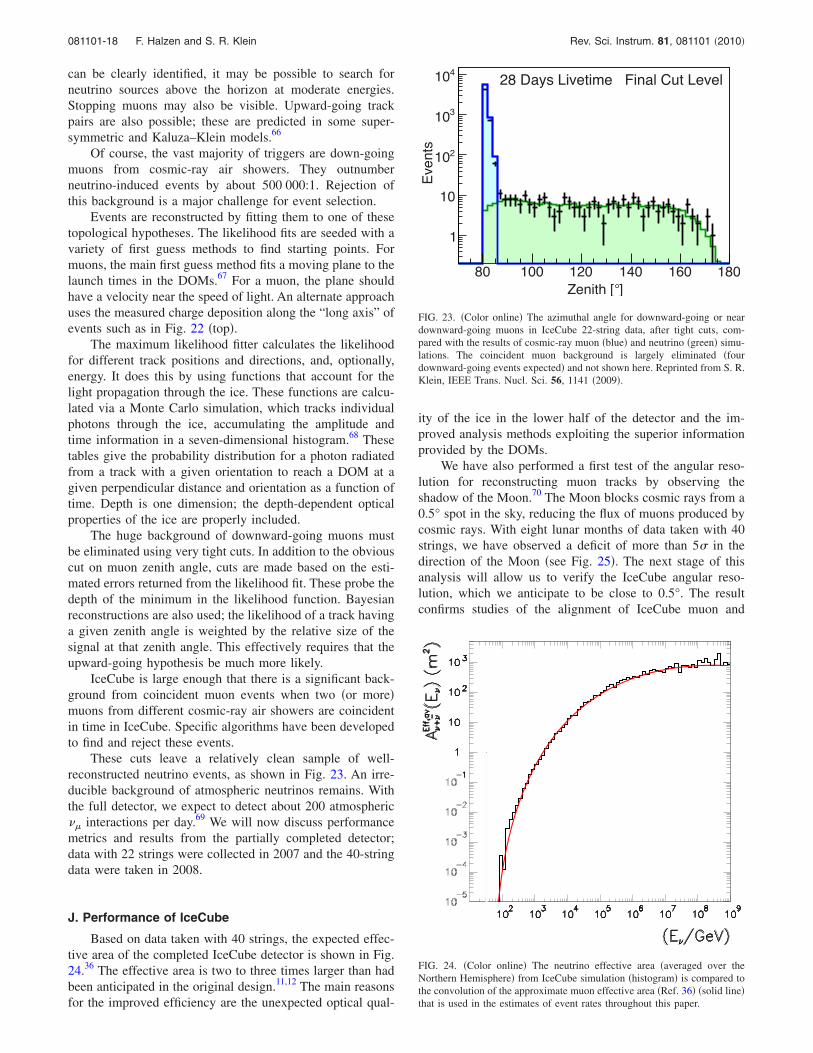
can be clearly identified, it may be possible to search forneutrino sources above the horizon at moderate energies.Stopping muons may also be visible. Upward-going trackpairs are also possible; these are predicted in some super-symmetric and Kaluza–Klein models.66
Of course, the vast majority of triggers are down-goingmuons from cosmic-ray air showers. They outnumberneutrino-induced events by about 500 000:1. Rejection ofthis background is a major challenge for event selection.
Events are reconstructed by fitting them to one of thesetopological hypotheses. The likelihood fits are seeded with avariety of first guess methods to find starting points. Formuons, the main first guess method fits a moving plane to thelaunch times in the DOMs.67 For a muon, the plane shouldhave a velocity near the speed of light. An alternate approachuses the measured charge deposition along the “long axis” ofevents such as in Fig. 22 �top�.
The maximum likelihood fitter calculates the likelihoodfor different track positions and directions, and, optionally,energy. It does this by using functions that account for thelight propagation through the ice. These functions are calcu-lated via a Monte Carlo simulation, which tracks individualphotons through the ice, accumulating the amplitude andtime information in a seven-dimensional histogram.68 Thesetables give the probability distribution for a photon radiatedfrom a track with a given orientation to reach a DOM at agiven perpendicular distance and orientation as a function oftime. Depth is one dimension; the depth-dependent opticalproperties of the ice are properly included.
The huge background of downward-going muons mustbe eliminated using very tight cuts. In addition to the obviouscut on muon zenith angle, cuts are made based on the esti-mated errors returned from the likelihood fit. These probe thedepth of the minimum in the likelihood function. Bayesianreconstructions are also used; the likelihood of a track havinga given zenith angle is weighted by the relative size of thesignal at that zenith angle. This effectively requires that theupward-going hypothesis be much more likely.
IceCube is large enough that there is a significant back-ground from coincident muon events when two �or more�muons from different cosmic-ray air showers are coincidentin time in IceCube. Specific algorithms have been developedto find and reject these events.
These cuts leave a relatively clean sample of well-reconstructed neutrino events, as shown in Fig. 23. An irre-ducible background of atmospheric neutrinos remains. Withthe full detector, we expect to detect about 200 atmospheric�� interactions per day.69 We will now discuss performancemetrics and results from the partially completed detector;data with 22 strings were collected in 2007 and the 40-stringdata were taken in 2008.
J. Performance of IceCube
Based on data taken with 40 strings, the expected effec-tive area of the completed IceCube detector is shown in Fig.24.36 The effective area is two to three times larger than hadbeen anticipated in the original design.11,12 The main reasonsfor the improved efficiency are the unexpected optical qual-
ity of the ice in the lower half of the detector and the im-proved analysis methods exploiting the superior informationprovided by the DOMs.
We have also performed a first test of the angular reso-lution for reconstructing muon tracks by observing theshadow of the Moon.70 The Moon blocks cosmic rays from a0.5° spot in the sky, reducing the flux of muons produced bycosmic rays. With eight lunar months of data taken with 40strings, we have observed a deficit of more than 5 in thedirection of the Moon �see Fig. 25�. The next stage of thisanalysis will allow us to verify the IceCube angular reso-lution, which we anticipate to be close to 0.5°. The resultconfirms studies of the alignment of IceCube muon and
]°Zenith [80 100 120 140 160 180
Events
1
10
210
310
410 28 Days Livetime Final Cut Level
FIG. 23. �Color online� The azimuthal angle for downward-going or neardownward-going muons in IceCube 22-string data, after tight cuts, com-pared with the results of cosmic-ray muon �blue� and neutrino �green� simu-lations. The coincident muon background is largely eliminated �fourdownward-going events expected� and not shown here. Reprinted from S. R.Klein, IEEE Trans. Nucl. Sci. 56, 1141 �2009�.
FIG. 24. �Color online� The neutrino effective area �averaged over theNorthern Hemisphere� from IceCube simulation �histogram� is compared tothe convolution of the approximate muon effective area �Ref. 36� �solid line�that is used in the estimates of event rates throughout this paper.
081101-18 F. Halzen and S. R. Klein Rev. Sci. Instrum. 81, 081101 �2010�
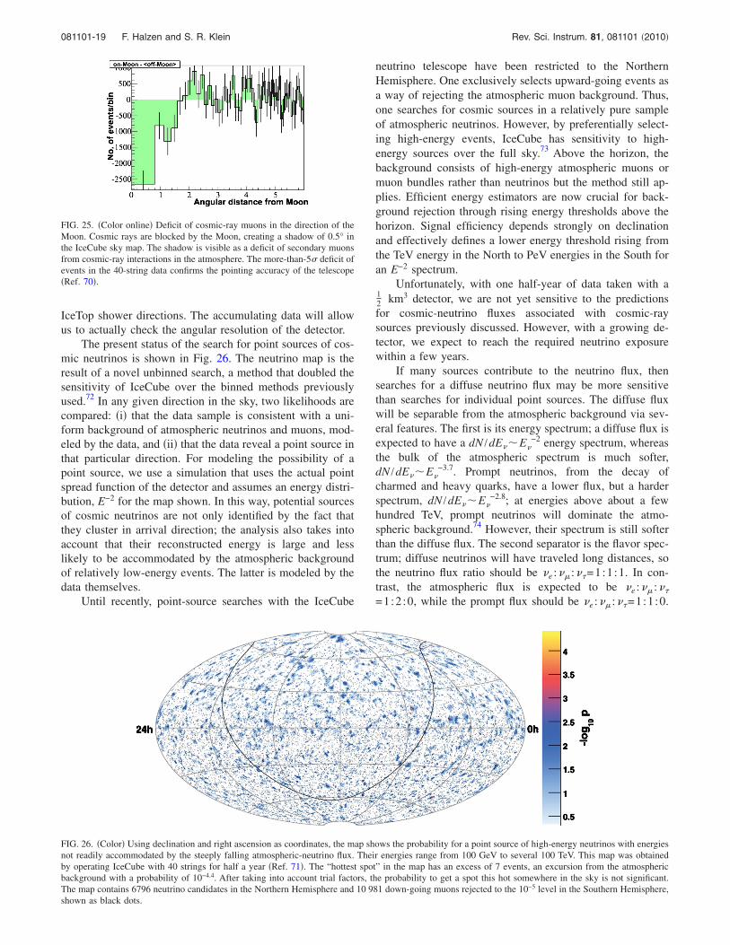
IceTop shower directions. The accumulating data will allowus to actually check the angular resolution of the detector.
The present status of the search for point sources of cos-mic neutrinos is shown in Fig. 26. The neutrino map is theresult of a novel unbinned search, a method that doubled thesensitivity of IceCube over the binned methods previouslyused.72 In any given direction in the sky, two likelihoods arecompared: �i� that the data sample is consistent with a uni-form background of atmospheric neutrinos and muons, mod-eled by the data, and �ii� that the data reveal a point source inthat particular direction. For modeling the possibility of apoint source, we use a simulation that uses the actual pointspread function of the detector and assumes an energy distri-bution, E−2 for the map shown. In this way, potential sourcesof cosmic neutrinos are not only identified by the fact thatthey cluster in arrival direction; the analysis also takes intoaccount that their reconstructed energy is large and lesslikely to be accommodated by the atmospheric backgroundof relatively low-energy events. The latter is modeled by thedata themselves.
Until recently, point-source searches with the IceCube
neutrino telescope have been restricted to the NorthernHemisphere. One exclusively selects upward-going events asa way of rejecting the atmospheric muon background. Thus,one searches for cosmic sources in a relatively pure sampleof atmospheric neutrinos. However, by preferentially select-ing high-energy events, IceCube has sensitivity to high-energy sources over the full sky.73 Above the horizon, thebackground consists of high-energy atmospheric muons ormuon bundles rather than neutrinos but the method still ap-plies. Efficient energy estimators are now crucial for back-ground rejection through rising energy thresholds above thehorizon. Signal efficiency depends strongly on declinationand effectively defines a lower energy threshold rising fromthe TeV energy in the North to PeV energies in the South foran E−2 spectrum.
Unfortunately, with one half-year of data taken with a12 km3 detector, we are not yet sensitive to the predictionsfor cosmic-neutrino fluxes associated with cosmic-raysources previously discussed. However, with a growing de-tector, we expect to reach the required neutrino exposurewithin a few years.
If many sources contribute to the neutrino flux, thensearches for a diffuse neutrino flux may be more sensitivethan searches for individual point sources. The diffuse fluxwill be separable from the atmospheric background via sev-eral features. The first is its energy spectrum; a diffuse flux isexpected to have a dN /dE��E�
−2 energy spectrum, whereasthe bulk of the atmospheric spectrum is much softer,dN /dE��E�
−3.7. Prompt neutrinos, from the decay ofcharmed and heavy quarks, have a lower flux, but a harderspectrum, dN /dE��E�
−2.8; at energies above about a fewhundred TeV, prompt neutrinos will dominate the atmo-spheric background.74 However, their spectrum is still softerthan the diffuse flux. The second separator is the flavor spec-trum; diffuse neutrinos will have traveled long distances, sothe neutrino flux ratio should be �e :�� :��=1:1 :1. In con-trast, the atmospheric flux is expected to be �e :�� :��
=1:2 :0, while the prompt flux should be �e :�� :��=1:1 :0.
FIG. 25. �Color online� Deficit of cosmic-ray muons in the direction of theMoon. Cosmic rays are blocked by the Moon, creating a shadow of 0.5° inthe IceCube sky map. The shadow is visible as a deficit of secondary muonsfrom cosmic-ray interactions in the atmosphere. The more-than-5 deficit ofevents in the 40-string data confirms the pointing accuracy of the telescope�Ref. 70�.
FIG. 26. �Color� Using declination and right ascension as coordinates, the map shows the probability for a point source of high-energy neutrinos with energiesnot readily accommodated by the steeply falling atmospheric-neutrino flux. Their energies range from 100 GeV to several 100 TeV. This map was obtainedby operating IceCube with 40 strings for half a year �Ref. 71�. The “hottest spot” in the map has an excess of 7 events, an excursion from the atmosphericbackground with a probability of 10−4.4. After taking into account trial factors, the probability to get a spot this hot somewhere in the sky is not significant.The map contains 6796 neutrino candidates in the Northern Hemisphere and 10 981 down-going muons rejected to the 10−5 level in the Southern Hemisphere,shown as black dots.
081101-19 F. Halzen and S. R. Klein Rev. Sci. Instrum. 81, 081101 �2010�
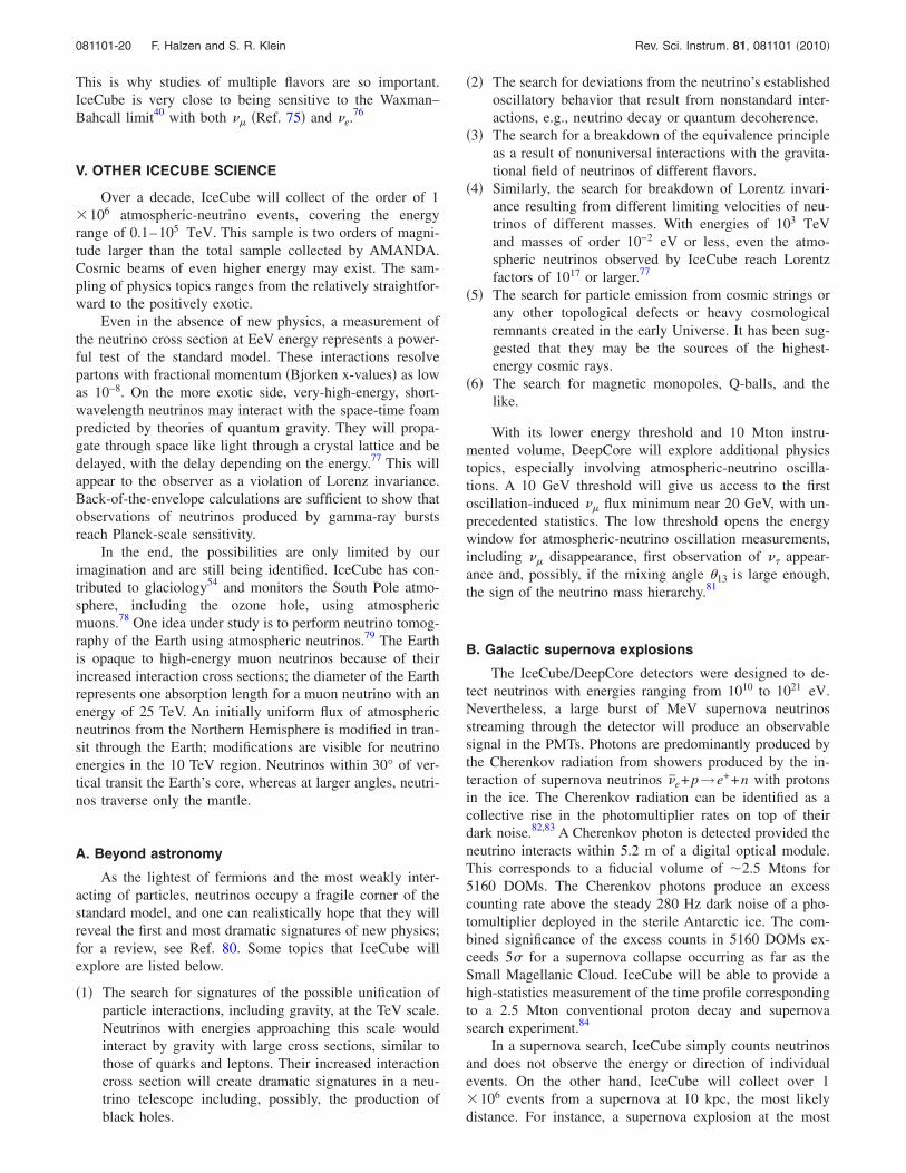
This is why studies of multiple flavors are so important.IceCube is very close to being sensitive to the Waxman–Bahcall limit40 with both �� �Ref. 75� and �e.
76
V. OTHER ICECUBE SCIENCE
Over a decade, IceCube will collect of the order of 1�106 atmospheric-neutrino events, covering the energyrange of 0.1–105 TeV. This sample is two orders of magni-tude larger than the total sample collected by AMANDA.Cosmic beams of even higher energy may exist. The sam-pling of physics topics ranges from the relatively straightfor-ward to the positively exotic.
Even in the absence of new physics, a measurement ofthe neutrino cross section at EeV energy represents a power-ful test of the standard model. These interactions resolvepartons with fractional momentum �Bjorken x-values� as lowas 10−8. On the more exotic side, very-high-energy, short-wavelength neutrinos may interact with the space-time foampredicted by theories of quantum gravity. They will propa-gate through space like light through a crystal lattice and bedelayed, with the delay depending on the energy.77 This willappear to the observer as a violation of Lorenz invariance.Back-of-the-envelope calculations are sufficient to show thatobservations of neutrinos produced by gamma-ray burstsreach Planck-scale sensitivity.
In the end, the possibilities are only limited by ourimagination and are still being identified. IceCube has con-tributed to glaciology54 and monitors the South Pole atmo-sphere, including the ozone hole, using atmosphericmuons.78 One idea under study is to perform neutrino tomog-raphy of the Earth using atmospheric neutrinos.79 The Earthis opaque to high-energy muon neutrinos because of theirincreased interaction cross sections; the diameter of the Earthrepresents one absorption length for a muon neutrino with anenergy of 25 TeV. An initially uniform flux of atmosphericneutrinos from the Northern Hemisphere is modified in tran-sit through the Earth; modifications are visible for neutrinoenergies in the 10 TeV region. Neutrinos within 30° of ver-tical transit the Earth’s core, whereas at larger angles, neutri-nos traverse only the mantle.
A. Beyond astronomy
As the lightest of fermions and the most weakly inter-acting of particles, neutrinos occupy a fragile corner of thestandard model, and one can realistically hope that they willreveal the first and most dramatic signatures of new physics;for a review, see Ref. 80. Some topics that IceCube willexplore are listed below.
�1� The search for signatures of the possible unification ofparticle interactions, including gravity, at the TeV scale.Neutrinos with energies approaching this scale wouldinteract by gravity with large cross sections, similar tothose of quarks and leptons. Their increased interactioncross section will create dramatic signatures in a neu-trino telescope including, possibly, the production ofblack holes.
�2� The search for deviations from the neutrino’s establishedoscillatory behavior that result from nonstandard inter-actions, e.g., neutrino decay or quantum decoherence.
�3� The search for a breakdown of the equivalence principleas a result of nonuniversal interactions with the gravita-tional field of neutrinos of different flavors.
�4� Similarly, the search for breakdown of Lorentz invari-ance resulting from different limiting velocities of neu-trinos of different masses. With energies of 103 TeVand masses of order 10−2 eV or less, even the atmo-spheric neutrinos observed by IceCube reach Lorentzfactors of 1017 or larger.77
�5� The search for particle emission from cosmic strings orany other topological defects or heavy cosmologicalremnants created in the early Universe. It has been sug-gested that they may be the sources of the highest-energy cosmic rays.
�6� The search for magnetic monopoles, Q-balls, and thelike.
With its lower energy threshold and 10 Mton instru-mented volume, DeepCore will explore additional physicstopics, especially involving atmospheric-neutrino oscilla-tions. A 10 GeV threshold will give us access to the firstoscillation-induced �� flux minimum near 20 GeV, with un-precedented statistics. The low threshold opens the energywindow for atmospheric-neutrino oscillation measurements,including �� disappearance, first observation of �� appear-ance and, possibly, if the mixing angle �13 is large enough,the sign of the neutrino mass hierarchy.81
B. Galactic supernova explosions
The IceCube/DeepCore detectors were designed to de-tect neutrinos with energies ranging from 1010 to 1021 eV.Nevertheless, a large burst of MeV supernova neutrinosstreaming through the detector will produce an observablesignal in the PMTs. Photons are predominantly produced bythe Cherenkov radiation from showers produced by the in-teraction of supernova neutrinos �̄e+ p→e++n with protonsin the ice. The Cherenkov radiation can be identified as acollective rise in the photomultiplier rates on top of theirdark noise.82,83 A Cherenkov photon is detected provided theneutrino interacts within 5.2 m of a digital optical module.This corresponds to a fiducial volume of �2.5 Mtons for5160 DOMs. The Cherenkov photons produce an excesscounting rate above the steady 280 Hz dark noise of a pho-tomultiplier deployed in the sterile Antarctic ice. The com-bined significance of the excess counts in 5160 DOMs ex-ceeds 5 for a supernova collapse occurring as far as theSmall Magellanic Cloud. IceCube will be able to provide ahigh-statistics measurement of the time profile correspondingto a 2.5 Mton conventional proton decay and supernovasearch experiment.84
In a supernova search, IceCube simply counts neutrinosand does not observe the energy or direction of individualevents. On the other hand, IceCube will collect over 1�106 events from a supernova at 10 kpc, the most likelydistance. For instance, a supernova explosion at the most
081101-20 F. Halzen and S. R. Klein Rev. Sci. Instrum. 81, 081101 �2010�
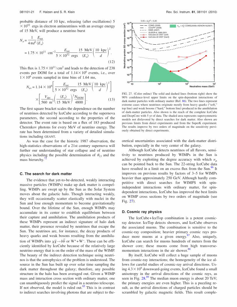
probable distance of 10 kpc, releasing �after oscillations� 5�1052 ergs in electron antineutrinos with an average energyof 15 MeV, will produce a neutrino burst
N� =1
4�d2
Etot
�E�
= 1.75 � 1011 cm−2 Etot
5 � 1052 ergs
15 MeV
�E� 10 kpc
d�2
.
�12�
This flux is 1.75�1011 /cm2 and leads to the detection of 238events per DOM for a total of 1.14�106 events, i.e., over1�106 events sampled in time bins of 1.64 ms,
Nev = 1.14 � 106� Etot
5 � 1052 ergs
15 MeV
�E� 10 kpc
d�2�
�� Vdet
560 m3 �E� 15 MeV
�3NDOM
4800� . �13�
The first square bracket scales the dependence on the numberof neutrinos detected by IceCube according to the supernovaparameters, the second according to the properties of thedetector. The event rate is based on a flux of 183 producedCherenkov photons for every MeV of neutrino energy. Therate has been determined from a variety of detailed simula-tions including GEANT.
As was the case for the historic 1987 observation, thehigh-statistics observations of a 21st century supernova willfurther our understanding of star collapse and of neutrinophysics including the possible determination of �13 and themass hierarchy.72
C. The search for dark matter
The evidence that yet-to-be-detected, weakly interactingmassive particles �WIMPs� make up dark matter is compel-ling. WIMPs are swept up by the Sun as the Solar Systemmoves about the galactic halo. Though interacting weakly,they will occasionally scatter elastically with nuclei in theSun and lose enough momentum to become gravitationallybound. Over the lifetime of the Sun, enough WIMPs mayaccumulate in its center to establish equilibrium betweentheir capture and annihilation. The annihilation products ofthese WIMPs represent an indirect signature of halo darkmatter, their presence revealed by neutrinos that escape theSun. The neutrinos are, for instance, the decay products ofheavy quarks and weak bosons resulting from the annihila-
tion of WIMPs into ��̄→bb̄ or W++W−. These can be effi-ciently identified by IceCube because of the relatively largeneutrino energy that is on the order of the mass of the WIMP.The beauty of the indirect detection technique using neutri-nos is that the astrophysics of the problem is understood. Thesource in the Sun has built up over solar time sampling thedark matter throughout the galaxy; therefore, any possiblestructure in the halo has been averaged out. Given a WIMPmass and interaction cross section with ordinary matter, onecan unambiguously predict the signal in a neutrino telescope.If not observed, the model is ruled out.85 This is in contrastto indirect searches involving photons that are subject to the-
oretical uncertainties associated with the dark-matter distri-bution, especially in the very center of the galaxy.
Although IceCube detects neutrinos of all flavors, sensi-tivity to neutrinos produced by WIMPs in the Sun isachieved by exploiting the degree accuracy with which ��
can be pointed back to the Sun. The 22-string IceCube datahave resulted in a limit on an excess flux from the Sun.86 Itimproves on previous results by factors of 3–5 for WIMPsheavier than approximately 250 GeV. Although hardly com-petitive with direct searches for WIMPS with spin-independent interactions with ordinary matter, for spin-dependent interactions, IceCube has improved the best limitson WIMP cross sections by two orders of magnitude �seeFig. 27�.
D. Cosmic ray physics
The IceCube+IceTop combination is a potent cosmic-ray detector. IceTop detects showers, and IceCube observesthe associated muons. The combination is sensitive to thecosmic-ray composition; heavier primary cosmic rays pro-duce more muons at a given energy.87 Also, uniquely,IceCube can search for muons hundreds of meters from theshower core; these muons come from high transverse-momentum interactions in the air shower.88
By itself, IceCube will collect a huge sample of muonsfrom cosmic-ray interactions; the homogeneity of the ice al-lows for careful studies of cosmic-ray arrival directions. Us-ing 4.3�109 downward-going events, IceCube found a smallanisotropy in the arrival directions of the cosmic rays, asseen in Fig. 28.89 The median muon energy is about 20 TeV;the primary energies are even higher. This is a puzzling re-sult, as the arrival directions of charged particles should bescrambled by galactic magnetic fields. This result comple-
Neutralino mass (GeV)10
210
310
410
)2
Ne
utr
alin
o-p
roto
nS
Dc
ros
s-s
ec
tio
n(c
m
-4110
-4010
-3910
-3810
-3710
-3610
-3510
-3410
-3310
CDMS(2008)+XENON10(2007)limSI
σ<SI
σ
< 0.202hχΩ0.05 <
CDMS (2008)COUPP (2008)KIMS (2007)
SUPER-K 1996-2001IceCube-22 2007 (soft)IceCube-22 2007 (hard)
102
103
104
10-4110
-4010
-3910
-3810
-3710
-3610
-3510
-3410
-3310
FIG. 27. �Color online� The solid and dashed lines �bottom right� show the90% confidence-level upper limits on the spin-dependent interactions ofdark matter particles with ordinary matter �Ref. 86�. The two lines representextreme cases where neutrinos originate mostly from heavy quarks �“soft,”top line� and weak bosons �“hard,” bottom line� produced in the annihilationof dark-matter particles. Also shown is the reach of the complete IceCubeand DeepCore with 5 yr of data. The shaded area represents supersymmetricmodels not disfavored by direct searches for dark matter. Also shown areprevious limits from direct experiments and from the SuperK experiment.The results improve by two orders of magnitude on the sensitivity previ-ously obtained by direct experiments.
081101-21 F. Halzen and S. R. Klein Rev. Sci. Instrum. 81, 081101 �2010�
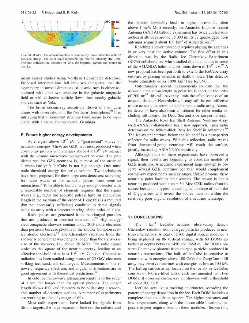
ments earlier studies using Northern Hemisphere detectors.Proposed interpretations fall into two categories: that theasymmetry in arrival directions of cosmic rays is either as-sociated with unknown structure in the galactic magneticfield or with diffusive particle flows from nearby galacticsources such as Vela.
The broad cosmic-ray anisotropy shown in the figurealigns with observations in the Northern Hemisphere.90 It isintriguing that a prominent structure there seems to be asso-ciated with a major photon source, Geminga.
E. Future higher-energy developments
At energies above 1017 eV, a “guaranteed” source ofneutrinos emerges. These are GZK neutrinos, produced whencosmic-ray protons with energies above 4�1019 eV interactwith the cosmic microwave background photons. The pre-dicted rate for GZK neutrinos is, at most, of the order of1 event /km3 yr−1; IceCube is not big enough. One musttrade threshold energy for active volume. Two techniqueshave been proposed for these large-area detectors: searchingfor radio waves or for acoustic pulses from neutrinointeractions.2 To be able to build a large enough detector witha reasonable number of elements requires that the signalwaves �e.g., radio and acoustic pulses� have an attenuationlength in the medium of the order of 1 km; this is a required�but not necessarily sufficient� condition to detect signalsusing an array with a detector spacing of the order of 1 km.
Radio pulses are generated from the charged particlesthat are produced in neutrino interactions.91 High-energyelectromagnetic showers contain about 20% more electronsthan positrons because photons in the shower Compton scat-ter atomic electrons.92 The Cherenkov radiation from theshower is coherent at wavelengths longer than the transversesize of the showers, i.e., above 20 MHz. The radio signalscales as the square of the neutrino energy, leading to aneffective threshold of at least 1017 eV. Coherent Cherenkovradiation has been studied using beams of 25 GeV electronsstriking ice, sand, and salt targets. Measurements of the rfpower, frequency spectrum, and angular distributions are ingood agreement with theoretical predictions.93
In cold ice, radio-wave attenuation length is of the orderof 1 km, far longer than for optical photons. The longerlength allows 100 km3 detectors to be built using a reason-able number of detection stations. A number of experimentsare working to take advantage of this.
Most radio experiments have looked for signals fromdistant targets; the large separation between the radiator and
the detector inevitably leads to higher thresholds, oftenabove 1 EeV. Most recently, the Antarctic Impulse TransitAntenna �ANITA� balloon experiment has twice circled Ant-arctica at altitudes around 35 000 m. Its 32 quad-ridged hornantennas scanned about 106 km3 of Antarctic ice.94
Reaching a lower threshold requires placing the antennasin or very near the active volume. The first effort in thisdirection was by the Radio Ice Cherenkov Experiment�RICE� collaboration, who installed dipole antennas in someof the AMANDA holes, and set limits down to 1017 eV.95 Anew proposal has been put forth to extend the IceCube arrayoutward by placing antennas in shallow holes. This detectorwould ultimately cover 1000 km3 �see Ref. 96�.
Unfortunately, recent measurements indicate that theacoustic attenuation length in polar ice is short, of the orderof 200 m;97 this will severely limit the effectiveness of anacoustic detector. Nevertheless, it may still be cost-effectiveto use acoustic detectors to supplement a radio array. Acous-tic detectors have also been considered for other media in-cluding salt domes, the Dead Sea and Siberian permafrost.
The Antarctic Ross Ice Shelf Antenna Neutrino Array�ARIANNA� collaboration has a new approach, using radiodetectors on the 650-m-thick Ross Ice Shelf in Antarctica.98
The ice-water interface below the ice shelf is a near-perfectreflector for radio waves. With this reflection, radio wavesfrom downward-going neutrinos will reach the surface,greatly increasing ARIANNA’s sensitivity.
Although none of these experiments have observed asignal, their results are beginning to constrain models ofGZK neutrinos. A neutrino experiment large enough to ob-serve several GZK neutrinos per year would complementcosmic-ray experiments such as Auger. Unlike protons, theseneutrinos point back to their sources. The reason is that aneutrino produced within an �50 Mpc GZK radius from itssource located at a typical cosmological distance of the orderof Gigaparsecs will reveal the source location within therelatively poor angular resolution of a neutrino telescope.
VI. CONCLUSIONS
The 1 km3 IceCube neutrino observatory detectsCherenkov radiation from charged particles produced in neu-trino interactions. A total of 5160 digital optical modules isbeing deployed on 86 vertical strings, with 60 DOMs at-tached at depths between 1450 and 2450 m. The DOMs ob-serve Cherenkov photons from charged particles produced inneutrino interactions. The bulk of IceCube is sensitive toneutrinos with energies above 100 GeV; the DeepCore infillarray may observe neutrinos with energies as low as 10 GeV.The IceTop surface array, located on the ice above IceCube,consists of 160 ice-filled tanks, each instrumented with twoDOMs. It observes cosmic-ray air showers with a thresholdof about 300 GeV.
IceCube acts like a tracking calorimeter, recording thepattern of energy deposition in the ice. Each DOM includes acomplete data acquisition system. The higher pressures andlow temperatures, along with the inaccessible locations, im-pose stringent requirements on these modules. Despite this,
FIG. 28. �Color� The arrival direction of cosmic-ray muons detected with 22IceCube strings. The color scale represents the relative intensity �Ref. 79�.The star indicates the direction of Vela, the brightest gamma-ray source inthe sky.
081101-22 F. Halzen and S. R. Klein Rev. Sci. Instrum. 81, 081101 �2010�
over 98% of the 4740 deployed modules are working per-fectly, with a global time resolution of about 2 ns.
Segmentation allows IceCube to separate ��, �e, and ��
interactions. We have developed reconstruction methods thateffectively separate upward-going muons from �� interac-tions from the much-more-intense cosmic-ray muon back-ground. These methods achieve an angular resolution of bet-ter than 1° for long tracks. The early data from IceCube areextremely promising, and the partial detector is now observ-ing over 10 000 neutrino events per year.
ACKNOWLEDGMENTS
We thank our IceCube collaborators for numerous dis-cussions on neutrino physics. We thank Evelyn Malkus andKim Krieger for helping with graphics and proofreading andJuan Carlos Diaz-Velez for the event displays in Fig. 22. Thiswork was funded in part by the National Science Foundationunder Grant Nos. 0653266, OPP-0236449, and PHY-0354776 and by the Department of Energy under ContractNo. DE-AC-76SF-00098.
1 F. Reines and C. L. Cowan, Jr., Nature �London� 178, 446 �1956�.2 F. Halzen and S. R. Klein, Phys. Today 61 �5�, 29 �2008�.3 A. Roberts, Rev. Mod. Phys. 64, 259 �1992�.4 T. K. Gaisser, F. Halzen, and T. Stanev, Phys. Rep. 258, 173 �1995�; 271,355�E� �1996�; e-print arXiv:hep-ph/9410384; J. G. Learned and K.Mannheim, Annu. Rev. Nucl. Part. Sci. 50, 679 �2000�; F. Halzen and D.Hooper, Rep. Prog. Phys. 65, 1025 �2002�.
5 M. A. Markov, in Proceedings of International Conference on High En-ergy Physics, 1960, edited by E. C. G. Sudarshan, J. H. Tinlot, and A. C.Melissinos �Rochester University Department of Physics, Interscience,New York, 1960�, p. 578.
6 J. Babson, B. Barish, R. Becker-Szendy et al., Phys. Rev. D 42, 3613�1990�.
7 BAIKAL Collaboration, V. A. Balkanov, I. Belolaptikov, N. Budnevet al., Nucl. Phys. B, Proc. Suppl. 118, 363 �2003�; BAIKAL Collabora-tion, V. Aynutdinov, A. Avrorin, V. Balkanov et al., Astropart. Phys. 25,140 �2006�.
8 NESTOR Collaboration, G. Aggouras, E. G. Anassontzis, A. E. Ball et al.,Astropart. Phys. 23, 377 �2005�.
9 ANTARES Collaboration, J. A. Aguilar, A. Albert, F. Ameli et al., Astro-part. Phys. 26, 314 �2006�.
10 E. Migneco, J. Phys.: Conf. Ser. 136, 022048 �2008�.11 IceCube Collaboration, “IceCube preliminary design document,” 2001,
available at http://www.icecube.wisc.edu/science/publications/pdd/pdd.pdf.
12 IceCube Collaboration, J. Ahrens, J. N. Bahcall, X. Bai et al., Astropart.Phys. 20, 507 �2004�; e-print arXiv:astro-ph/0305196.
13 F. Halzen, Eur. Phys. J. C 46, 669 �2006�.14 S. R. Klein for the IceCube Collaboration, IEEE Trans. Nucl. Sci. 56,
1141 �2009�.15 A. Karle for the IceCube Collaboration, Proceedings of the 31st Interna-
tional Cosmic Ray Conference, Lodz, Poland, 2009.16 J. Carr, F. Cohen, D. Dornic, F. Jouvenot, G. Maurin, and C. Naumann for
the KM3NeT Consortium, J. Phys.: Conf. Ser. 136, 042063 �2008�.17 T. Kajita and Y. Totsuka, Rev. Mod. Phys. 73, 85 �2001�.18 R. Davis, Rev. Mod. Phys. 75, 985 �2003�.19 MACRO Collaboration, M. Calicchio, G. Case, C. Demarzo et al., Nucl.
Instrum. Methods Phys. Res. A 264, 18 �1988�.20 G. Giacomelli and A. Margiotta, e-print arXiv:0707.1691.21 Fréjus Collaboration, W. Rhode, K. Daum, P. Bareyre et al., Astropart.
Phys. 4, 217 �1996�.22 IMB Collaboration, R. Bionta, G. Blewitt, C. B. Bratton et al., Phys. Rev.
Lett. 58, 1494 �1987�.23 Kamiokande Collaboration, K. Hirata, T. Kajita, M. Koshiba et al., Phys.
Rev. Lett. 58, 1490 �1987�.24 Super-Kamiokande Collaboration, Y. Fukuda, T. Hayakawa, E. Ichihara
et al., Nucl. Instrum. Methods Phys. Res. A 501, 418 �2003�.
25 SNO Collaboration, J. Boger, R. L. Hahn, J. K. Rowley et al., Nucl.Instrum. Methods Phys. Res. A 449, 172 �2000�.
26 IceCube Collaboration, R. Abassi et al., e-print arXiv:1004.2357; IceCubeCollaboration, A. Achterberg, M. Ackermann, J. Adams et al., Phys. Rev.D 76, 042008 �2007�.
27 J. K. Becker, Phys. Rep. 458, 173 �2008�; e-print arXiv:0710.1557.28 R. Engel, D. Seckel, and T. Stanev, Phys. Rev. D 64, 093010 �2001�;
e-print arXiv:astro-ph/0101216 and references therein.29 See M. Ahlers, L. A. Anchordoqui, M. C. Gonzalez-Garcia, F. Halzen, and
S. Sarkar, e-print arXiv:1005.2620 for a recent discussion and referencestherein.
30 P. Sommers and S. Westerhoff, e-print arXiv:0802.1267; A. M. Hillas,e-print arXiv:astro-ph/0607109; V. Berezinsky, e-print arXiv:0801.3028.
31 F. Halzen, e-print arXiv:0910.0436.32 W. Baade and F. Zwicky, Phys. Rev. 46, 76 �1934�.33 MILAGRO Collaboration, A. A. Abdo, B. Allen, D. Berley et al., Astro-
phys. J. Lett. 658, L33 �2007�; e-print arXiv:astro-ph/0611691.34 For a recent discussion, see S. Gabici and F. A. Aharonian, Astrophys. J.
Lett. 665, L131 �2007�; e-print arXiv:0705.3011.35 F. Halzen, A. Kappes, and A. O’Murchadha, Phys. Rev. D 78, 063004
�2008�; e-print arXiv:0803.0314.36 M. C. Gonzalez-Garcia, F. Halzen, and S. Mohapatra, Astropart. Phys. 31,
437 �2009�; e-print arXiv:0902.1176.37 E. Waxman, Phys. Rev. Lett. 75, 386 �1995�; e-print arXiv:astro-ph/
9701231.38 M. Vietri, Phys. Rev. Lett. 80, 3690 �1998�; e-print arXiv:astro-ph/
9802241.39 F. W. Stecker and M. H. Salamon, Astrophys. J. 512, 521 �1999�; e-print
arXiv:astro-ph/9808110.40 E. Waxman and J. N. Bahcall, Phys. Rev. D 59, 023002 �1999�; e-print
arXiv:hep-ph/9807282.41 E. Waxman and J. N. Bahcall, Phys. Rev. Lett. 78, 2292 �1997�; e-print
arXiv:astro-ph/9701231.42 D. Guetta, D. Hooper, J. Alvarez-Muñizm, F. Halzen, and E. Reuveni,
Astropart. Phys. 20, 429 �2004�; e-print arXiv:astro-ph/0302524.43 J. G. Learned and S. Pakvasa, Astropart. Phys. 3, 267 �1995�; e-print
arXiv:hep-ph/9405296.44 F. Halzen and D. Saltzberg, Phys. Rev. Lett. 81, 4305 �1998�; e-print
arXiv:hep-ph/9804354.45 E. Middell, J. McCartin, and M. D’Agostino for the IceCube Collabora-
tion, Proceedings of the 31st International Cosmic Ray Conference, Lodz,Poland, 2009.
46 S. R. Klein, e-print arXiv:astro-ph/0412546; Radiat. Phys. Chem. 75, 696�2006�.
47 D. Cowen for the IceCube Collaboration, J. Phys.: Conf. Ser. 60, 227�2007�; T. DeYoung, S. Razzaque, and D. F. Cowen, Astropart. Phys. 27,238 �2007�.
48 AMANDA Collaboration, E. Andrés, P. Askebjer, X. Bai et al., Nature�London� 410, 441 �2001�.
49 AMANDA Collaboration, M. Ackermann, J. Ahrens, X. Bai et al., Nucl.Instrum. Methods Phys. Res. A 556, 169 �2006�.
50 C. Wiebusch for the IceCube Collaboration, e-print arXiv:0907.2263.51 T. Stanev for the IceCube Collaboration, Nucl. Phys. B, Proc. Suppl. 196,
159 �2009�.52 L. Demirors, e-print arXiv:0711.0353.53 AMANDA Collaboration, M. Ackermann, J. Ahrens, X. Bai et al., J.
Geophys. Res. 111, D13203, doi:10.1029/2005JD006687 �2006�.54 N. E. Bramall, R. C. Bay, K. Woschnagg, R. A. Rohde, and P. B. Price,
Geophys. Res. Lett. 32, L21815, doi:10.1029/2005GL024236 �2005�.55 K. Hanson and O. Tarasova for the IceCube Collaboration, Nucl. Instrum.
Methods Phys. Res. A 567, 214 �2006�.56 R. Abbasi, Y. Abdou, T. Abu-Zayyad et al., Nucl. Instrum. Methods Phys.
Res. A 618, 139 �2010�; e-print arXiv:1002.2442.57 EMCO Corporation, see M. Doherty, M. Janto, and M. Helmreich, Pho-
tonics Spectra 1, 58 �2005�.58 S. Klein for the IceCube Collaboration, e-print arXiv:astro-ph/0601269.59 IceCube Collaboration, R. Abbasi, M. Ackermann, J. Adams et al., Nucl.
Instrum. Methods Phys. Res. A 601, 294 �2009�.60 S. Kleinfelder, IEEE Trans. Nucl. Sci. 50, 955 �2003�.61 R. G. Stokstad for the IceCube Collaboration, presented at the 11th Work-
shop on Electronics for LHC and Future Electronics, Heidelberg, Ger-many, 12–16 September 2005.
62 IceCube Collaboration, A. Achterberg, M. Ackermann, J. Adams et al.,Astropart. Phys. 26, 155 �2006�.
081101-23 F. Halzen and S. R. Klein Rev. Sci. Instrum. 81, 081101 �2010�

63 J. Kiryluk et al. for the IceCube Collaboration, e-print arXiv:0711.0353.64 A. Gross et al. for the IceCube Collaboration, e-print arXiv:0711.0353.65 J. Pretz, Ph.D. dissertation, University of Maryland, 2006.66 I. Albuquerque and S. Klein, Phys. Rev. D 80, 015015 �2009�.67 AMANDA Collaboration, J. Ahrens, X. Bai, R. Bay et al., Nucl. Instrum.
Methods Phys. Res. A 524, 169 �2004�.68 J. Lundberg, P. Miočinović, K. Woschnagg, T. Burgess, J. Adams, S. Hun-
dertmark, P. Desiati, and P. Niessen, Nucl. Instrum. Methods Phys. Res. A581, 619 �2007�.
69 S. R. Klein for the IceCube Collaboration, e-print arXiv:0810.0573.70 D. J. Boersma for the IceCube Collaboration, Proceedings of the 31st
International Cosmic Ray Conference, Lodz, Poland, 2009.71 J. Dumm for the IceCube Collaboration, Proceedings of the 31st Interna-
tional Cosmic Ray Conference, Lodz, Poland, 2009.72 J. Braun, J. Dumm, F. De Palma, C. Finley, A. Karle, and T. Montaruli,
Astropart. Phys. 29, 299 �2008�; e-print arXiv:0801.1604.73 IceCube Collaboration, R. Abbasi, Y. Abdou, T. Abu-Zayyad et al., Phys.
Rev. Lett. 103, 221102 �2009�; e-print arXiv:0911.2338.74 R. Enberg, M. H. Reno, and I. Sarcevic, Phys. Rev. D 78, 043005 �2008�.75 K. Hultqvist for the IceCube Collaboration, e-print arXiv:1003.2300.76 J. Kiryluk for the IceCube Collaboration, e-print arXiv:0909.0989.77 IceCube Collaboration, R. Abbasi, Y. Abdou, M. Ackermann et al., Phys.
Rev. D 79, 102005 �2009�.78 S. Tilav et al., Proceedings of the 31st International Cosmic Ray Confer-
ence, Lodz, Poland, 2009.79 M. C. Gonzalez-Garcia, F. Halzen, M. Maltoni, and H. K. M. Tanaka,
Phys. Rev. Lett. 100, 061802 �2008�; e-print arXiv:0711.0745.80 See M. C. Gonzalez-Garcia, F. Halzen, and M. Maltoni, Phys. Rev. D 71,
093010 �2005�; e-print arXiv:hep-ph/0502223 and references therein.81 D. Grant and J. Koskinen for the IceCube Collaboration, Proceedings of
the 31st ICRC, 2009.82 F. Halzen, J. Jacobsen, and E. Zas, Phys. Rev. D 53, 7359 �1996�; see also
A. S. Dighe, M. T. Keil, and G. G. Raffelt, J. Cosmol. Astropart. Phys.0306, 006 �2003�.
83 AMANDA Collaboration, J. Ahrens, X. Bai, G. Barouch et al., Astropart.Phys. 16, 345 �2002�.
84 IceCube Collaboration, R. Abbasi, Y. Abdou, T. Abu-Zayyad et al.,“IceCube sensitivity for low-energy neutrinos from nearby supernovae,”Astrophys. J. �unpublished�.
85 F. Halzen and D. Hooper, New J. Phys. 11, 105019 �2009�; e-printarXiv:0910.4513.
86 IceCube Collaboration, A. Abbasi, Y. Abdou, M. Ackermann et al., Phys.Rev. Lett. 102, 201302 �2009�; e-print arXiv:0902.2460; J. Braun and D.Hubert for the IceCube Collaboration, Proceedings of the 31st ICRC,2009, Paper No. HE2.3; e-print arXiv:0906.1615.
87 T. Feussels, C. Xu, and J. Eisch for the IceCube Collaboration, Proceed-ings of the 31st ICRC, 2009.
88 L. Gerhardt and S. Klein for the IceCube Collaboration, e-printarXiv:0909.0055; S. Klein, Nucl. Phys. A 830, 869c �2009�.
89 R. Abbasi and P. Desiati for the IceCube Collaboration, e-printarXiv:0907.0498.
90 Super-Kamiokande Collaboration, G. Guillian, J. Hosaka, K. Ishiharaet al., Phys. Rev. D 75, 062003 �2007�; Tibet AS Gamma Collaboration,M. Amenomori, S. Ayabe, X. J. Bi et al., Science 314, 439 �2006�; FermiLAT Collaboration, A. Abdo, B. T. Allen, T. Aune et al., Astrophys. J.698, 2121 �2009�; J. L. Zhang, Y. Zhang, S. W. Cui, and Ch. Fan, onbehalf of the ARGO-YBJ Collaboration, Proceedings of the 31st ICRC,Lodz, 2009.
91 For a review, see F. Halzen, J. Phys.: Conf. Ser. 120, 062004 �2008�;e-print arXiv:0710.4158 and references therein.
92 G. A. Askarian, Sov. Phys. JETP 14, 441 �1962�.93 ANITA Collaboration, P. W. Gorham, S. W. Barwick, J. J. Beatty et al.,
Phys. Rev. Lett. 99, 171101 �2007�.94 ANITA Collaboration, P. W. Gorham, P. Allison, B. M. Baughman et al.,
e-print arXiv:1003.2961; ANITA Collaboration, P. W. Gorham, P. Allison,S. W. Barwick et al., Phys. Rev. Lett. 103, 051103 �2009�.
95 RICE Collaboration, I. Kravchenko, C. Cooley, S. Hussain et al., Phys.Rev. D 73, 082002 �2006�.
96 P. Allison, J. Beatty, P. Chen et al., Nucl. Instrum. Methods Phys. Res. A604, S64 �2009�; e-print arXiv:0904.1309.
97 F. Descamps for the IceCube Collaboration, Proceedings of the 31stICRC, 2009.
98 L. Gerhardt, S. R. Klein, T. Stezelberger et al. e-print arXiv:1005.5193; S.Barwick, Nucl. Instrum. Methods Phys. Res. A 602, 279 �2009�.
081101-24 F. Halzen and S. R. Klein Rev. Sci. Instrum. 81, 081101 �2010�


![Neutrino source search with Four year IceCube neutrino …...Neutrino source search with Four year IceCube neutrino events. Reetanjali Moharana & Soebur Razzaque [University of Johannesburg]](https://static.fdocuments.us/doc/165x107/60bfab986073fe01ea4f136a/neutrino-source-search-with-four-year-icecube-neutrino-neutrino-source-search.jpg)