INVITED PAPER Cyber–PhysicalModelingof ...

INV ITEDP A P E R

Cyber–Physical Modeling ofDistributed Resources forDistribution SystemOperationsThe Virtual Grid Integration Laboratory (VirGIL) is a modular cosimulation

platform designed to study interactions between demand-response

strategies, building comfort, communication networks, and power system

operation. VirGIL introduces the use of the quantized state system (QSS)

methods for simulation in this cosimulation platform.

By Spyros Chatzivasileiadis, Member IEEE, Marco Bonvini, Javier Matanza,

Rongxin Yin, Thierry S. Nouidui, Emre C. Kara, Member IEEE, Rajiv Parmar,

David Lorenzetti, Michael Wetter, and Sila Kiliccote, Member IEEE

ABSTRACT | Cosimulation platforms are necessary to study

the interactions of complex systems integrated in future smart

grids. The Virtual Grid Integration Laboratory (VirGIL) is a

modular cosimulation platform designed to study interactions

between demand-response (DR) strategies, building comfort,

communication networks, and power system operation. This

paper presents the coupling of power systems, buildings,

communications, and control under a master algorithm. There

are two objectives: first, to use a modular architecture for

VirGIL, based on the functional mockup interface (FMI),

where several different modules can be added, exchanged,

and tested; and second, to use a commercial power system

simulation platform, familiar to power system operators, such

as DIgSILENT PowerFactory. This will help reduce the barriers

to the industry for adopting such platforms, investigate and

subsequently deploy DR strategies in their daily operation.

VirGIL further introduces the integration of the quantized

state system (QSS) methods for simulation in this cosimulation

platform. Results on how these systems interact using a real

network and consumption data are also presented.

KEYWORDS | Cosimulation; demand response (DR); DigSILENT

PowerFactory; functional mockup interface (FMI); load flow;

modelica; OMNeT++

I . INTRODUCTION

Moving toward “smarter” grids, power system complexity

increases through the embedding of communication net-

works, demand-side management, electric vehicles, and

the stochastic nature of several renewable energy sources(RES). Simulation platforms specialized in power sys-

tems can no longer handle in an adequate way the in-

creasing interdependencies with systems such as

communications, buildings, and electric vehicles. More

detailed simulation tools are necessary to study the sys-

tem interdependencies and determine the appropriate

control strategies for optimizing power system operation.

An option is to extend the existing power system simula-tion tools by incorporating the dynamics of such net-

works inside the same simulation platform. On the other

hand, research in the respective fields has developed

highly detailed and reliable tools, which can simulate the

behavior and control of such systems. This paper adopts

the cosimulation approach, where highly developed and

reliable simulation tools, specialized in the respective

Manuscript received February 15, 2015; revised October 9, 2015; acceptedOctober 26, 2015. Date of publication March 7, 2016; date of current versionMarch 17, 2016. This work was supported by the Laboratory Directed Research andDevelopment (LDRD) funding from Berkeley Laboratory, provided by the Director,Office of Science, of the U.S. Department of Energy DE-AC02-05CH11231.S. Chatzivasileiadis is with the Massachusetts Institute of Technology (MIT),Cambridge, MA 02139 USA (e-mail: [email protected]).M. Bonvini is with Whiskerlabs, Oakland, CA 94612 USA (e-mail:[email protected]).J. Matanza is with Comillas Pontifical University, Madrid 28015, Spain (e-mail:[email protected]).R. Yin, T. S. Nouidui, E. C. Kara, D. Lorenzetti, and M. Wetter are with theLawrence Berkeley National Laboratory, Berkeley, CA 94720 USA (e-mail: [email protected]; [email protected]; [email protected]; [email protected]; [email protected]).R. Parmar is with the University of Calgary, Calgary, AB T1Y 4Z9, Canada and alsowith the Lawrence Berkeley National Laboratory, Berkeley, CA 94720 USA (e-mail:[email protected]).S. Kiliccote is with the SLAC National Accelerator Laboratory, Menlo Park, CA 94025USA (e-mail: [email protected]).

Digital Object Identifier: 10.1109/JPROC.2016.2520738

0018-9219 Ó 2016 IEEE. Personal use is permitted, but republication/redistribution requires IEEE permission.See http://www.ieee.org/publications_standards/publications/rights/index.html for more information.

Vol. 104, No. 4, April 2016 | Proceedings of the IEEE 789

fields, are merged in a common cosimulation platform tostudy the interdependencies between systems and iden-

tify appropriate control strategies.

Although cosimulation has found a lot of applications

in, e.g., the automotive industry or building controls

(e.g., BCVTB [1]), in power systems it is a relatively re-

cent field which has seen some development during the

last eight years. The approach followed in this paper is to

couple a commercial power system simulation platform,widely used by power system operators, with advanced

modeling tools for buildings and communication net-

works. The goal is to determine the impact the demand-

response (DR) strategies have on the network and

determined optimal algorithms to utilize flexible loads

for power system operation.

Two are the main objectives. First, we aim at reduc-

ing the barriers for adoption of novel DR and other con-trol strategies in the daily power system operation.

Coupling a trusted power system simulator, with which

several power system operators are familiar, with other

advanced modeling tools will help toward a wider adop-

tion of such tools. Testing and becoming familiar with

the impact of different strategies on the power system

will allow the wider deployment and utilization of the

energy reserves “stored” in buildings, e.g., in the form ofthermal inertia. Second, we need a modular cosimulation

architecture, which will allow the easy exchange and test

of different simulation modules, as well as the easy ex-

tension with, e.g., electric vehicle simulators, optimiza-

tion tools, hardware-in-the-loop, etc. For this reason, we

use the functional mockup interface (FMI) standard,

which provides a standardized interface for the coupling

of several different tools.This paper describes the Virtual Grid Integration

Laboratory (VirGIL), which couples a commercial power

system simulator with models for buildings and commu-

nication networks. The goal is to estimate the impact of

DR strategies on the grid, and to determine optimal algo-

rithms for exploiting flexible loads (for example, the

thermal energy stored in buildings).

VirGIL’s architecture is based on the FMI, which de-fines a standard interface for exposing the capabilities of

a simulation tool [3]. FMI, which is an open industrial

standard, provides for a modular structure that allows

the simple exchange and testing of different cosimulation

tools. VirGIL is implemented using the CyPhySim distri-

bution of the Ptolemy II framework, which combines

mechanisms for continuous time, discrete time, and

discrete-event simulation, and quantized state system(QSS) integrators and FMIs [4], [5].

VirGIL is implemented in the Ptolemy II frame-

work, which combines continuous and discrete-event

simulation [4].

This paper is organized as follows. Section II reviews

existing cosimulation methods in power systems.

Section III provides the overview of the proposed

cosimulation architecture in VirGIL, while Section IVdescribes the FMI. Sections V–VIII present, respectively,

the development of the power systems, buildings, com-

munications, and control functional mockup units

(FMUs). Sections IX and X describe the simulation of

the model exchange FMUs based on the QSS algorithm

and the operation of the master algorithm, respectively.

Section XI describes simulation results based on real

data for the LBNL network. Finally, Section XII con-cludes this paper and provides an outlook for future ex-

tensions of this work.

II . COSIMULATION IN POWER SYSTEMS

Over the last years, several cosimulation approaches for

power systems have been developed and documented in

the literature. One of the first documented efforts is [6],which cosimulates power and communication systems.

The authors advocate the use of already existing simula-

tion tools that excel in their respective fields instead of

creating new simulation platforms (“federated ap-

proach”). In that work, power systems are simulated with

fixed step through PSCAD/EMTDC and PSLF while com-

munication simulations are carried out on the discrete

event simulator ns-2. The two tools are synchronized atspecific “synchronization points” without an implementa-

tion for a rollback function, which results in accumula-

tion of synchronization induced inacurracies over time.

The authors improved this approach in [7] where they

use a master algorithm with a common timeline for both

modules. There are no “synchronization points,” instead

both simulators evolve synchronously in time.

Most of the cosimulation approaches for power sys-tems combine power system with communication net-

work simulation (examples for distribution networks are

[8] and [9]). Stifter et al. [10] report a cosimulation ap-

proach for power systems and EV charging and control,

where they also use FMI for the coupling of one of the

simulation tools to the master algorithm. A survey of the

latest simulation tools that are used for cosimulation in

power systems is reported, among others, in [11].This work focuses on the interactions of building

models for energy consumption with distribution system

models for power system operation.

Among the tools used for cosimulation, Gridlab-D is

probably one of the most widespread [12]. It has a flexi-

ble environment, which incorporates advanced modeling

techniques, efficient simulation algorithms, but most im-

portantly provide a simulation environment not only forpower systems, but also incorporating detailed load

modeling, rate structure analysis, distributed generator,

and distribution automation.

In this paper, a commercial power system software,

DigSilent PowerFactory, is used for power system simula-

tion. Building a cosimulation platform incorporating

PowerFactory, a tool that several utilities trust and use in

790 Proceedings of the IEEE | Vol. 104, No. 4, April 2016

Chatzivasileiadis et al. : Cyber–Physical Modeling of Distributed Resources for Distribution System Operations

their daily operation, decreases the barriers for wideradoption of cosimulation tools from the industry. Power

system operators can incorporate their version of Power-

Factory with the cosimulation platform to investigate in

more detail the effect of DR signals, decide and subse-

quently deploy the most appropriate in real-time opera-

tion. PowerFactory has the additional advantage of being

capable to model both alternating current (ac) and direct

current (dc) systems. A cosimulation approaches incorpo-rating PowerFactory has also been documented in [13].

However, this is the first time that a modular cosimula-

tion architecture, based on FMI, is implemented for cou-

pling PowerFactory with the rest of the simulation tools.

Besides the development of the appropriate models

and controls within each simulation tool, the focus in

this paper is on the development of the wrapper func-

tions which will make the modules compatible to theFMI standard for cosimulation. FMI provides for a mod-

ular structure of the cosimulation platform which allows

the simple exchange and testing of different cosimulation

tools. VirGIL’s master algorithm will be Ptolemy II,

which can combine both continuous and discrete-event

simulation. At the same novel simulation algorithms are

implemented in Ptolemy II, such as QSS which allow for

higher efficiency and faster execution times.

III . VirGIL

VirGIL is a modular cosimulation platform that currently

couples models of power systems, buildings, communica-

tions, and has the potential to integrate other sources or

sinks on the electrical grid, including electric vehicles.The platform will facilitate developing novel control al-

gorithms, and optimizing power systems, buildings,

communications, and EV charging.

Fig. 1 shows an overview of the VirGIL cosimulation

architecture.

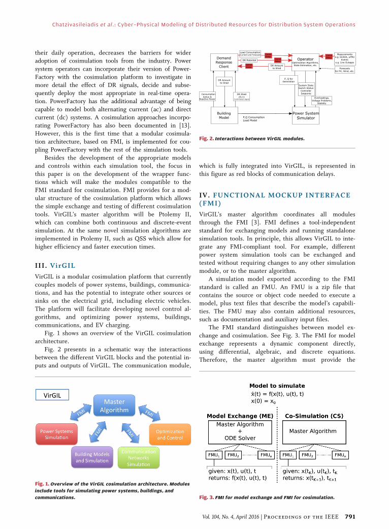
Fig. 2 presents in a schematic way the interactions

between the different VirGIL blocks and the potential in-

puts and outputs of VirGIL. The communication module,

which is fully integrated into VirGIL, is represented in

this figure as red blocks of communication delays.

IV. FUNCTIONAL MOCKUP INTERFACE(FMI)

VirGIL’s master algorithm coordinates all modules

through the FMI [3]. FMI defines a tool-independent

standard for exchanging models and running standalone

simulation tools. In principle, this allows VirGIL to inte-

grate any FMI-compliant tool. For example, differentpower system simulation tools can be exchanged and

tested without requiring changes to any other simulation

module, or to the master algorithm.

A simulation model exported according to the FMI

standard is called an FMU. An FMU is a zip file that

contains the source or object code needed to execute a

model, plus text files that describe the model’s capabili-

ties. The FMU may also contain additional resources,such as documentation and auxiliary input files.

The FMI standard distinguishes between model ex-

change and cosimulation. See Fig. 3. The FMI for model

exchange represents a dynamic component directly,

using differential, algebraic, and discrete equations.

Therefore, the master algorithm must provide the

Fig. 1. Overview of the VirGIL cosimulation architecture. Modules

include tools for simulating power systems, buildings, and

communications.

Fig. 2. Interactions between VirGIL modules.

Fig. 3. FMI for model exchange and FMI for cosimulation.



necessary solvers. By contrast, the FMI for cosimulationdefines an interface for coupling independent simulation

tools. Under cosimulation, the FMU itself provides the

associated solvers. In both cases, the master algorithm

coordinates time, and exchanges inputs and outputs,

between FMUs.

VirGIL can integrate both types of FMU. For exam-

ple, the power system model uses the FMI for cosimula-

tion, while the buildings model uses the FMI for modelexchange.

V. POWER SYSTEM FMU

After reviewing several power system software packages,

we chose DigSILENT PowerFactory as the power system

simulator. The main focus was on established commer-

cial power system software, in order to demonstratehow cosimulation enables the use of familiar specialized

simulation tools. For this project, PowerFactory’s script-

ing interfaces, for example, to C++, C#, Python, and

Matlab/Simulink, made it especially attractive. In our im-

plementation, all VirGIL modules, except for the power

system part run on Linux. DigSILENT PowerFactory runs

only on Windows. As a result, we implemented a socket

communication between Windows and Linux. In Linuxthe PowerFMU implements all functions necessary for

the FMI standard and calls their counterpart in the

Windows implementation through the socket. The

Windows FMU, in turn, calls the Python functions that

start and stop PowerFactory, parameterize the simula-

tion, set the inputs, and get the outputs.

Fig. 4 shows the structure of the FMU for power sys-

tem simulation. The FMU maps the C-language functionsdefined in the FMI standard to calls on PowerFactory’s

Python API. For example:

• fmi2Instantiate(): start PowerFactory, Activate

Project;

• fmi2SetReal(), fmi2SetInteger(), fmi2SetString():Set the values of variables and parameters;

• fmi2DoStep(): execute load flow;

• fmi2GetReal(), fmi2GetInteger(), fmi2GetString():Get the values of variables and parameters.

VirGIL’s initial focus is on the impact of DR algo-

rithms in the power system steady-state operation, e.g.,

to investigate line loadings and voltage profiles. Thus,

the power system FMU runs several sequential load

flows, and determines the state of the system after each

run. Extending the FMU to handle dynamic simulationsis an object of future work.

VI. BUILDINGS FMU

To study how DR affects the distribution grid, VirGIL

requires a building model that can capture the relevant

dynamics, without placing undue computational burden

on the overall simulation. For example, the model shouldhave sufficient detail to show the effect of DR strategies

such as changing temperature setpoints, or reducing fan

speeds.

Building energy performance depends on the interac-

tion between many heterogeneous elements, e.g., the en-

velope, windows, lighting, controls, and the heating

ventilation and air-conditioning (HVAC) systems. To rep-

resent these elements, the building model used in VirGILcomprises four main parts, as shown in Fig. 5: 1) the

thermal system that describe the envelope, windows, in-

terior slabs and partitions, and room air; 2) the HVAC

systems (e.g., air handling units, fans, etc.); 3) a set of

schedules that describe thermal/electric loads such as

lights, plug loads and internal heat gains generated by

occupants; and 4) the building control systems thatFig. 4. An FMU wrapper for PowerFactory. The arrows represent

variable names.

Fig. 5. Overview of the virgil building FMU model. The model

comprises four main parts: the building thermal model, the HVAC

system, the schedules, and the control system.



manages the HVAC and other assets in order to maintain

the comfort levels and receives DR signals.

While VirGIL could incorporate EnergyPlus models

directly, using its FMI interface for cosimulation [14], a

complete EnergyPlus model is too detailed to simulate

all the buildings in a complete distribution system. The

building resistance–capacitance modeling (BRCM) tool-

box [15] provides an alternative to overcome the compu-tational burden of a full-building simulation model such

EnergyPlus. The BRCM toolbox constitutes a part of the

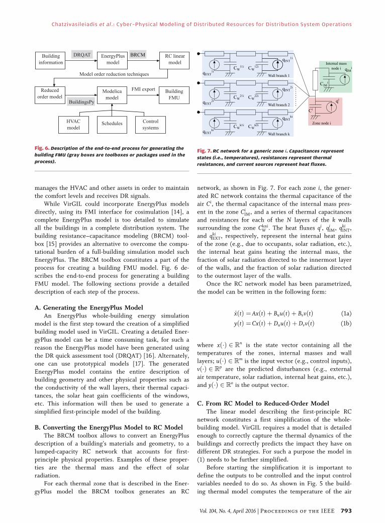
process for creating a building FMU model. Fig. 6 de-

scribes the end-to-end process for generating a building

FMU model. The following sections provide a detailed

description of each step of the process.

A. Generating the EnergyPlus ModelAn EnergyPlus whole-building energy simulation

model is the first step toward the creation of a simplified

building model used in VirGIL. Creating a detailed Ener-

gyPlus model can be a time consuming task, for such a

reason the EnergyPlus model have been generated using

the DR quick assessment tool (DRQAT) [16]. Alternately,

one can use prototypical models [17]. The generated

EnergyPlus model contains the entire description ofbuilding geometry and other physical properties such as

the conductivity of the wall layers, their thermal capaci-

tances, the solar heat gain coefficients of the windows,

etc. This information will then be used to generate a

simplified first-principle model of the building.

B. Converting the EnergyPlus Model to RC ModelThe BRCM toolbox allows to convert an EnergyPlus

description of a building’s materials and geometry, to a

lumped-capacity RC network that accounts for first-

principle physical properties. Examples of these proper-

ties are the thermal mass and the effect of solar

radiation.

For each thermal zone that is described in the Ener-

gyPlus model the BRCM toolbox generates an RC

network, as shown in Fig. 7. For each zone i, the gener-

ated RC network contains the thermal capacitance of the

air Ci, the thermal capacitance of the internal mass pres-

ent in the zone CiIM, and a series of thermal capacitances

and resistances for each of the N layers of the k walls

surrounding the zone CkniW . The heat fluxes qi, qiIM, q

kiINT,

and qkiEXT, respectively, represent the internal heat gains

of the zone (e.g., due to occupants, solar radiation, etc.),the internal heat gains heating the internal mass, the

fraction of solar radiation directed to the innermost layer

of the walls, and the fraction of solar radiation directed

to the outermost layer of the walls.

Once the RC network model has been parametrized,

the model can be written in the following form:

_xðtÞ ¼ AxðtÞ þ BuuðtÞ þ BvvðtÞ (1a)

yðtÞ ¼ CxðtÞ þ DuuðtÞ þ DvvðtÞ (1b)

where xð�Þ 2 Rn is the state vector containing all thetemperatures of the zones, internal masses and wall

layers; uð�Þ 2 Rm is the input vector (e.g., control inputs),

vð�Þ 2 Rp are the predicted disturbances (e.g., external

air temperature, solar radiation, internal heat gains, etc.),

and yð�Þ 2 Ro is the output vector.

C. From RC Model to Reduced-Order ModelThe linear model describing the first-principle RC

network constitutes a first simplification of the whole-

building model. VirGIL requires a model that is detailed

enough to correctly capture the thermal dynamics of thebuildings and correctly predicts the impact they have on

different DR strategies. For such a purpose the model in

(1) needs to be further simplified.

Before starting the simplification it is important to

define the outputs to be controlled and the input control

variables needed to do so. As shown in Fig. 5 the build-

ing thermal model computes the temperature of the air

Fig. 6. Description of the end-to-end process for generating the

building FMU (gray boxes are toolboxes or packages used in the

process).

Fig. 7. RC network for a generic zone i. Capacitances represent

states (i.e., temperatures), resistances represent thermal

resistances, and current sources represent heat fluxes.



in the zones that is then returned to the HVAC systemðTRETÞ. The local controller controls the HVAC system in

order to maintain the temperature of the air in the build-

ing as close as possible to the desired setpoint. The

HVAC system model computes the cooling power to be

delivered to maintain the zone temperatures at the de-

sired setpoint.

This description allows to introduce two simplifica-

tions. First, the HVAC and the control system are notpart of the building thermal model. They interact with a

suitable representation of the building that given the in-

ternal heat gains and the other known disturbances com-

putes the return temperature. This allows to remove the

HVAC inputs uð�Þ from the model in (1). Second, the

output vector yð�Þ is equal to the return temperature

TRET, which is the weighted average of the thermal zones

temperature. After introducing such simplifications, (1)can be rewritten as

_xðtÞ ¼ AxðtÞ þ BvvðtÞ (2a)

yðtÞ ¼ CxðtÞ (2b)

C ¼ V1VTOT

� � � VnxVTOT

0 � � � 0

� �(2c)

where C 2 R1 � Rn is the output matrix, nz is the num-

ber of thermal zones [the first nz elements of the statevector xð�Þ], Vi for i 2 ½1; nz� is the volume of the iththermal, and VTOT ¼

Pnzi¼1 Vi is the sum of all the vol-

umes. The vector of known disturbances vð�Þ and outputs

yð�Þ are thus defined as

vð�Þ ¼ ðQIHG TAMB TGND SE SW SN SSÞTyð�Þ ¼ ðTRETÞ:

Here, QIHG is the heat flux from internal heat gains,

TAMB is the ambient temperature, TGND is the ground

temperature, and SE; SW ; SN; SS is the solar radiation from

east, west, north, and south, respectively.

Despite the fact that the number of input–outputrelationships of model (2) is seven, the number of

state variables can be high enough that the simulation

speed remains an issue (e.g., a model with ten zones

can easily have more than a hundred states). For such

a reason the model can be further reduced [18], [19].

As we describe in Section XI-A, the resulting model

will have a close match of the input–output behavior

while reducing the number of states.

D. Conversion to Modelica and Generationof the FMU

Once the reduced-order model that defines the input–

output relationships between the known disturbances

and the output is defined, it is possible to express itusing Modelica, an object-oriented, equation-based lan-

guage for modeling multidomain physical systems.

Then, drawing on the Modelica Buildings Library

[20], we add the HVAC, loads, and controls logic. These

components predict the active power consumption of the

building, and implement a DR system that adjusts the

zone temperatures and airflow setpoints according to DR

signals sent by the utility.Finally, we export the Modelica building model as an

FMU for model exchange.

VII. COMMUNICATION FMU

With respect to the communication modeling, OMNeT++

[21] was chosen among a number of simulation tools. This

open-source discrete event environment is a general com-munication simulator widely used in the research and ac-

ademic community. In this framework, a basic model is

built in a hierarchical manner: first the behavior of simple

modules is described in C++; then, these modules are in-

stantiated and tied together using OMNeT++’s network

description language (NED) in order to form more com-

plex entities.

Since OMNeT++’s main classes are mainly focusedon the implementation of the discrete event machine

and the simulation scheduler, it is common to add a

number of extensions to the framework in order to up-

grade the capability of the model. This is the case of the

INET framework, which includes support for IPv4, IPv6,

TCP, Ethernet, HTTP, and many other used protocols

within the Internet. Additionally, there exist other

frameworks that implement mobility scenarios (likeVNS), wireless sensor network (like WiXiM or Castalia),

LTE technology (like SimuLTE), etc. INET counts the all

the technologies that are needed for current version of

VirGIL.

Other simulator options considered were: ns-2/ns-3

(Network Simulator 2/Network Simulator 3), JiST (Java

in Simulation Time) and OPNET Modeler R. From

them, OMNeT++ and ns-2/ns3 have extensively beenused in cosimulation application for smart grid scenarios

[22]–[24]. Several reasons led us to choose OMNeT++.

From a technical perspective, OMNeT++ has shown

good agreement with measured data for a number of

communication technologies. This is the case of WiFi

(IEEE802.11g) or LTE, as reported in [25] and [26], re-

spectively. In terms of performance, both ns-2/ns-3 and

OMNeT++ have a similar performance and offer goodscalability features, as discussed in [27]. Further benefits

of OMNeT++ which help substantially in the implemen-

tation, are its extensive and detailed documentation, and

its integrated development environment adapted to

Eclipse which simplifies debugging.

Regarding the DR application under study, the model

counts with three high-level types of actors: server



nodes, where information about DR events is stored; cli-

ent nodes, which try to retrieve this information; and a

network, which interconnects all nodes. From a logicalperspective, the DR communication infrastructure can be

built using these three actors.

Both clients and servers in the network under study

will implement Open Automated Demand Response

(OpenADR) as an application layer protocol for exchang-

ing messages. OpenADR is a standardized communica-

tion data model for sending and receiving DR signals

from a utility or independent system operator to electriccustomers [28], [29].

Fig. 8 shows a more detailed scheme of the model.

The three already mentioned actors can be seen in the

figure: an OpenADR server, an OpenADR client, and an

interconnected network (in this case the Internet). Addi-

tionally, the figure also shows the implementation of the

different communication layers on each of the nodes. In

this case, the de facto Internet’s layer stack is chosen:TCP as a transport protocol, IP as network protocol, and

Ethernet as a physical protocol. OpenADR servers and

clients use the lower layers to transmit their information.

This layered structure, in practice, produces a virtual di-

rect communication between pairs of layers.

Additionally, Fig. 8 shows the names that OpenADR’

specification gives to the different nodes in the network:

virtual end nodes (VEN) and virtual top nodes (VTN).Information flows from VTN to VEN. Additionally, a

VEN may also behave as a VTN in order to forward cer-

tain data to other nodes.

The implementation of the network is shown in

Fig. 9. It counts with a DR server (labeled with

“serv”), a DR client (labeled with “cli½0�”), a number

or routers, and a cloud network. This scheme represents

the communication of both nodes in an interconnected

wired network such as the Internet. The figure only

shows one client for clarity reasons; however, the num-

ber of clients is a parameter for the model. In case that

more than one should exist, each one of them would

have its own router to connect to the cloud.Routers pretend to simulate the gateway that each In-

ternet service provider (ISP) would provide to a customer

in order to connect to the Internet; as such, routers only

implement up to layer-3 capabilities. The cloud network

models the Internet as a network with a variable delay,

transmission speed, and error rate. Recalling the classifi-

cation made in [24] about the network model’s level of

detail: the Internet would be modeled as a black-box com-munication network, whereas the rest of the entities

would count with a high level of detail (i.e., all layers and

communication processes are taken into account).

The structure of the FMU for the communication

model is shown in Fig. 10. The FMU acts as an interface

for the OMNeT++’s API. This API talks directly to the

simulation kernel in order to set or get certain variable’s

values or messages. In addition to INET, the kernel alsouses an additional library developed for this study where

other capabilities (such as the OpenADR server and cli-

ent) have been implemented.

At the current implementation of VirGIL, three types

of messages are exchanged between the server and the

client: the “load consumption,” the “DR potential” of the

load, and the “shed load request.” “Load consumption”

Fig. 8. Communication’s layer stack diagram.

Fig. 9. OMNeT++ implementation of the network.



and “DR potential,” along with their node identifier, aretransmitted from the client nodes to the server node.

The communication FMU simulates the message trans-

mission and, after the calculated communication delay, it

produces the output to the server. While “consumption”

and “DR potential” flow in one direction only, communi-

cation for DR events flows in both ways. The server node

sends a “shed load request” message to specified clients.

Upon reception, the client replies to the server whetherhe will participate in the DR event. The communication

FMU is responsible for transmitting these messages with

the appropriate latency.

It may happen that, due to errors in the transmission,

some of these messages get lost. However, these lost

messages are identified by the automatic repeat request

(ARQ) mechanism implemented on the TCP layer of all

nodes (see Fig. 8). Without going into too much detailabout ARQ, whenever a message is lost, a retransmission

mechanism is triggered at the transmitting party. The

result is that messages are always delivered even in the

presence of errors. The only effect is that erroneous

messages are affected by a higher latency (due to the

retransmission).

VIII. OPTIMIZATION ANDCONTROL FMU

The control and optimization FMU is responsible for

monitoring the status of the interconnected systems, and

issuing control signals if certain limits are violated. In

most of the cases, the control FMU monitors the power

system FMU and sends signals to change the electricity

demand in buildings, operate energy storage, etc. VirGILcan integrate many different control algorithms, ranging

from simple rule-based control, to more sophisticated

control laws, and optimization. The control blocks can

either be directly implemented in Ptolemy or integrated

through an FMI interface. For example, advanced optimi-

zation functions, which the owner would prefer to avoid

sharing the source code, can be wrapped in an FMU and

imported in VirGIL. In future versions, advanced optimalpower flow algorithms including convex relaxations will

be integrated.

The control and optimization FMU, depending on the

functions it carries out, may include a model of the

power system or of other components within VirGIL

(e.g., buildings). Still, the existence of a separate FMU

for power system simulation (and buildings, etc.) re-

mains necessary. For example, the power system FMUcontains a detailed power system model and is based on

commercial software that the operator uses and trusts.

Depending on the implementation, the power system

FMU could also include direct SCADA signals for switch-

ing operations, etc. As a result, it can determine with

much higher confidence the current and future status of

the power system. On the other hand, although the con-

trol and optimization FMU might as well include amodel of the power system (e.g., in case of an optimal

power flow algorithm), the level of accuracy and detail

would not necessarily be as high as in the power system

FMU. In control and optimization, we are mostly inter-

ested in arriving to good solutions (e.g., through convex

relaxations) and at the same time having a tractable

problem, and low computation times. Toward these ef-

forts, we may introduce simplifications to our models.Therefore, it is necessary for the power system FMU to

confirm that the determined control actions result to a

feasible and reasonable operating point.

For the use cases presented in this paper, we have

implemented two controllers: 1) a power system loading

controller, which monitors the loading of cables and

transformers, and if this exceeds a certain threshold it is-

sues a DR signal (see Section XI-C); and 2) a volt/varcontroller, which appropriately controls the reactive

power injection of a battery storage to track a voltage ref-

erence signal (see Section XI-D). First efforts have also

been carried out for a ramp-rate controller, where a bat-

tery storage assists in the reduction of steep power in-

creases or decreases, and, thus, reduces the need for

dispatching expensive power reserves. This will be pre-

sented in future work.

IX. TIME INTEGRATION OFDIFFERENTIAL EQUATIONS USINGQSS METHODS

As described in Section IV, each building’s FMU defines

ordinary differential equations of the form

_x ¼ fðx; u; tÞ (3)

where _xðtÞ is a vector of N state variables whose values

the solver will predict; uðtÞ is a vector of input variables

which act as boundary conditions; and f is the derivative

Fig. 10. Structure for the communication FMU.



function. If Ptolemy coordinates more than one suchFMU, then the state variables predicted by one FMU

may appear as the input variables of another.

To integrate these equations, we implemented both

explicit and linearly implicit QSS methods in Ptolemy

[30], [31]. QSS differs from typical integration methods,

in that it discretizes the state variables rather than time.

Thus, (3) becomes

_x ¼ fðq; �; tÞ (4)

where qðtÞ is the quantized state, i.e., a discretized ver-sion of xðtÞ. Likewise, �ðtÞ is a quantized version of uðtÞ.

Quantization consists of representing a variable as a

series of piecewise-continuous polynomials. Component jof the ODE system has a quantized state model

bqj½‘�ðtÞ ¼ XM�1

i¼0

q½i�j½‘� t� t

qj½‘�

� �i

(5)

where q½i�j½‘� denotes the ith polynomial coefficient for the

‘th model; tqj½‘� gives the quantization-event time at which

the model was formed; and M gives the QSS method or-

der. For example, QSS1, a first-order method, quantizes

the state as a constant, bqj½‘�ðtÞ ¼ bq ½0�j½‘� . Each model holds

on to tqj½‘� � t G t

qj½‘þ1� (although t

qj½‘þ1� is not known at

time tqj½‘�).

Integrating the quantized state gives a series of state

models

bxj½k�ðtÞ ¼ XMi¼0

x½i�j½k� t� tsj½k�� i

(7)

valid on tsj½k� � t � tsj½kþ1�. Note that the state-event times

tsj½k� may differ from the quantization-event times. Fig. 11

shows a block diagram of a QSS integrator.

Component j forms a new state model when a quan-tized input to fj changes. At the kth state-event time, the

new state model is made continuous with the previous

one, and its slope found from the derivative function

x½0�j½k� ¼ xj½k�1� tsj½k�

� �(7)

x½1�j½k� ¼ fj bq½��; b�½��; tsj½k�

� �� (8)

where the models bq½�� and b�½�� are evaluated at tsj½k�. Index“�” indicates the most recent model for each component.

For QSS2 and QSS3, the higher order coefficients x2j½k� andx3j½k� are estimated by perturbing the arguments to the deriv-ative function; details are beyond the scope of this paper.

Component j forms a new quantized state model

when the current quantized state model differs from bxj½k�by an amount �Qj, called the quantum. In the absence

of other events, this happens when

bxj½k� bt qj½‘þ1��

� bqj½‘� bt qj½‘þ1�� ¼ �Qj (9)

where bt qj½‘þ1� is the predicted quantization-event time for

component j. In practice, �Qj varies with the magnitude

of bq½0�j½k�, according to user-defined tolerances.

At each time step, the simulation advances to theminimum predicted quantization-event time from among

all the components. Thus, a given global time step may

requantize only one out of all the components.

When component j does finally experience a quantiza-

tion event, it forms a new quantized state model by match-

ing the value and derivatives from the current state model

q½0�j½‘� ¼bxj½k� t

qj½‘�

� �(10)

q½1�j½‘� ¼

dbxj½k�dt

tqj½‘�

� �(11)

and so on, for derivatives up to M� 1 (however, the line-

arly implicit QSS methods offset the initial value by up to

�Qj). The new quantized state model is then broadcast to

any other component whose derivative function depends

on xj. This, in turn, induces state events in those down-stream components.

Fig. 12 shows the QSS1 and QSS2 solutions of the ex-

ponential problem _x ¼ �x with initial condition

xð0Þ ¼ 1. Quantum was chosen as the minimum of 0.001

and 0:001 � jq½0�½‘� j. Compared to the analytical result

x ¼ e�t, both solutions end at t ¼ 3 with a global error

less than 5 � 10�4.

Fig. 11. QSS integration of a component of an ODE system. The

quantized state is a piecewise-continuous approximation to x(t).

The simulation iteratively updates the state and quantized state

models for individual components.



The QSS approach treats every differential equation

as a discrete event actor, generating events, and respond-

ing to the events produced by other equations. However,

the Ptolemy implementation currently groups the equa-

tions by FMU. Thus, if one equation experiences a state

event, it updates the state models for all equations con-

tained in the same FMU.In addition to the differential equations defined by

model exchange FMUs, Ptolemy also must handle cosimu-

lation FMUs. As suggested by Fig. 4, the power system

FMU defines a static relation, determining the power flows

as an algebraic function of its inputs. Since all feedback

paths from the power system outputs back to its inputs

pass through the building models, Ptolemy does not have

to solve any algebraic loops. To avoid having to call thepower FMU every time a building model updates one of its

outputs, we sample the building loads at discrete intervals.

X. MASTER ALGORITHM

To synchronize the data of the different FMUs, we will

use Ptolemy II [4]. Ptolemy II is a modular software en-vironment for the design and analysis of heterogeneous

systems. It provides a graphical model building environ-

ment, synchronizes the exchanged data, and visualizes

the system evolution during runtime. In Ptolemy II, com-

ponents are encapsulated as actors which communicate

with other actors through ports. A director orchestrates

the data exchange between the actors and advances time

for the individual actors.Next, we will discuss the mathematical structure of

each FMU, and then discuss how we composed them for

a cosimulation. To compose multiple actors in order to

conduct a cosimulation, we need to make the distinction

between outputs of actors that directly depend on inputs,

e.g., they have direct feedthrough, and outputs of actors

that do not directly depend on inputs. The latter are, for

example, outputs of explicit time integrators that onlychange when time is advanced, but not if an input is

changed.

The power system FMU implements an algebraic,

time-invariant system. Therefore, the outputs of this

FMU directly depend on the input values.

The building FMUs take as an input the control sig-

nal yshed and produce as outputs the active and reactive

power P and Q. Both do not directly depend on yshed.The building FMUs are exported using the FMI for

model-exchange 2.0 standard. When imported to

Ptolemy II, they are combined with QSS integrator, as

described in Section IX. For the master algorithms, these

QSS integrators can be abstracted as actors that may

schedule a time event whenever their input changes, or

whenever their state variables change by more than a

tolerance. Should the input change prior to such ascheduled event, then the actor may replace this event

with a new one that may happen at a different time.

The communication FMUs lead to time delays in the

signals. They take signal ujðtÞ as inputs, for some

j 2 f1; . . . ; ng, where n is a fixed number of channels,

and produce the signal at the output after some time de-

lay �jðtÞ. Hence, the output is yjðtþ �jðtÞÞ ¼ ujðtÞ. For

signal j, the time delay is a function of all signals thathave not yet been sent to their output, allowing to model

network congestion. In our communication FMU, once

�jðtÞ has been computed, it will not be changed. There-

fore, network congestion does not affect signals that

have already been received in the communication FMU

but have not yet been produced at its output.

The optimization and control FMU has discrete time

semantics. For a constant time step � > 0, and givenmeasurement signal uði�Þ, with i 2 f0; 1; . . .g, it outputsthe control action yððiþ 1Þ�Þ ¼ fðuði�ÞÞ.

Fig. 13 shows the Ptolemy II system model that com-

bines the power, building, communication, and control

FMU. The QSS director is a new addition to Ptolemy II

that we developed in conjunction with the Ptolemy II de-

velopment team. The QSS director extends the discrete

event director, and adds a QSS solver. Thereby, this di-rector allows combining FMUs for model exchange,

which will be integrated with the QSS algorithm, with

FMUs for cosimulation. In addition, other Ptolemy II ac-

tors that work in the discrete event domain can be used

in such system models.

Such a cyber–physical system has component subsys-

tems that operate with varying time scales. In our model,

the power system FMU is currently running as a se-quence of steady states (sequential power flows), while

the communication and control FMUs are running as

discrete-event simulations. In future work, we will also

enable dynamic simulations for the power system FMU.

The building FMU is originally a continuous dynamic

model, but through our QSS implementation we can run

it as an event-based system, decoupling the fast from the

Fig. 12. QSS solution of the exponential problem x = –x.



slow dynamics, e.g., change of HVAC electric power

(fast) versus change in building thermal mass tempera-

ture (slow). As a result, the building model is evaluated

when its DR signal changes or when the QSS algorithm

requires a new evaluation. Converting the continuous-

time semantics to discrete event semantics through the

use of QSS allows us to update the states of these subsys-tems at the rate required by their respective dynamics.

XI. SIMULATION RESULTS

A. Calibration of the Building ModelTo demonstrate VirGIL, we used a real building in-

side the Lawrence Berkeley National Laboratory (LBNL)campus. LBNL building 71 is a 54000-ft2 two story steel-

frame office and laboratory building located in Berkeley,

CA, USA. The building has a water-cooled chiller system

with three cooling towers. The building’s operation is

typical of office and laboratory, with an operational

schedule of 9:00 A.M. to 6:00 P.M. and high equipment

usage during off hours. The peak electric power demand

is over 400 kW during the period of 12:00 P.M. to 6:00P.M. and the average demand during the off hours is

about 80 kW.

The building FMU has been generated as described

in Section VI. Before using the building FMU model we

performed a calibration of the model in order to test

the ability of the simplified RC model to replicate the

results of the more detailed EnergyPlus model. Here,

we have assumed that the EnergyPlus model is already

calibrated against real measured data. As long as enough

sensor data become available, the EnergyPlus model is

calibrated based on the procedure documented in [16].

The main difference between the EnergyPlus model and

the simplified RC model are the nonlinear relationships

and complex algorithm used by EnergyPlus to computeinterior and exterior convective coefficients, solar heat

gain coefficients, and long wave radiation effects. How-

ever, the RC model has a number of coefficients that

can be tuned in order to align the simulation results as

much as possible. Sensitivity analysis was conducted to

rank the key parameters of the RC model that could be

tuned. The parameters with higher sensitivity that were

used to tune the model are: exterior wall convective co-efficient, building solar absorption factor, window heat

gain factor, and heat transmission value. We therefore

used the summer period from May to October to per-

form a comparison between the RC and the EnergyPlus

models. We decided to use such a period because it is

of interest for the DR events as well as for critical peak

pricing.

Both the RC and EnergyPlus models have been simu-lated using standard weather for San Francisco, lighting,

plug loads, occupancy, and setpoint schedules for the

zones of the building. Given the same boundary condi-

tion and operation the models predicted the cooling load

required to satisfy the required comfort conditions.

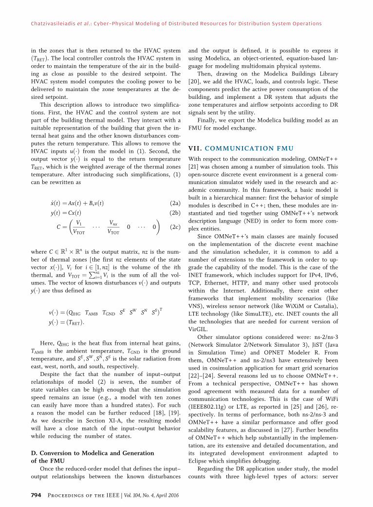
Fig. 14 shows the RC model cooling load versus the

EnergyPlus model cooling load. Every points represents a

Fig. 13. Ptolemy II model that shows the composition of the different FMUs.



simulated data point with a 5-min resolution over the

period between May and October. The green, yellow,

and red areas, respectively, represent a relative error of

�5%, �10%, and �15%. As can be seen, the highest

relative error occurs at low cooling load level while

when the load is close to its maximum the almost totality

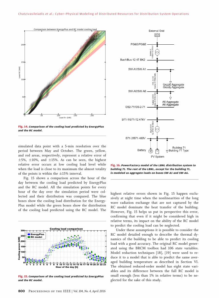
of the points is within the �15% interval.Fig. 15 shows a comparison across the hour of the

day between the cooling load predicted by EnergyPlus

and the RC model. All the simulation points for every

hour of the day over the simulation period were col-

lected and their distribution was compared. The blue

boxes show the cooling load distribution for the Energy-

Plus model while the green boxes show the distribution

of the cooling load predicted using the RC model. The

highest relative errors shown in Fig. 15 happen exclu-

sively at night time when the nonlinearities of the long

wave radiation exchange that are not captured by the

RC model dominate the heat transfer of the building.

However, Fig. 15 helps us put in perspective this error,

confirming that even if it might be considered high in

relative terms, its impact on the ability of the RC model

to predict the cooling load can be neglected.Under these assumptions it is possible to consider the

RC model detailed enough to describe the thermal dy-

namics of the building to be able to predict its cooling

load with a good accuracy. The original RC model gener-

ated using the BRCM toolbox had 106 state variables.

Model reduction techniques [18], [19] were used to re-

duce it to a model that is able to predict the same aver-

aged building temperature as described in Section VI.The obtained reduced-order model has eight state vari-

ables and its difference between the full RC model is

small enough (less than 1% in relative terms) to be ne-

glected for the sake of this study.

Fig. 14. Comparison of the cooling load predicted by EnergyPlus

and the RC model.

Fig. 15. Comparison of the cooling load predicted by EnergyPlus

and the RC model.

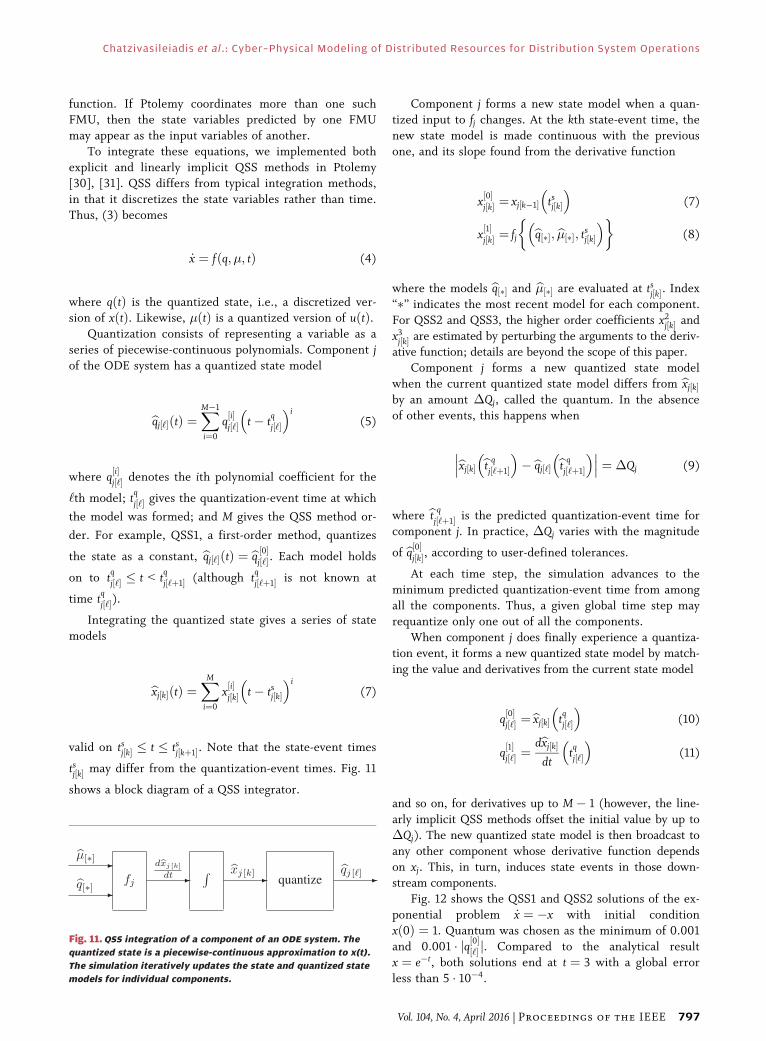
Fig. 16. PowerFactory model of the LBNL distribution system to

building 71. The rest of the LBNL, except for the building 71,

is modeled as aggregate loads on buses SW-A1 and SW-A6.



B. Overview of the Use CasesBoth cases use the LBNL distribution network and

building 71. As shown in Fig. 16, the LBNL distribution

network represents the path from the point of common

coupling with PG&E, down to building 71. The remain-

der of the distribution system loads are modeled as ag-gregated loads connected to two switching substations

along this path. Real 15-min data were used for the two

aggregate loads. For bus SW-A1, real reactive power was

used, while for SW-A6, a power factor of 0.94 induc-

tive was assumed. The active power consumptions of

the aggregate loads in SW-A1 and SW-A6 are shown in

Fig. 17.

The modeling of building 71 has been detailed inSection XI-A. To study the interaction of loads during

high penetration of DER, we have assumed a solar PV

plant of 340 kWp and a battery connected at the same

bus. The active power consumption of building 71 and

the net load (building 71 and solar PV) demanded at

bus B71 is shown in Fig. 18. As we did not have avail-

able data for the reactive power consumption of build-

ing 71, we assumed a constant power factor of 0.96

inductive.We present two use cases in the following sections to

demonstrate the capabilities of VirGIL. The first applies to

DR actions in building 71 to reduce the cable and trans-

former loading. The second applies to volt/var control so

that the voltage at bus B71 follows specified setpoints.

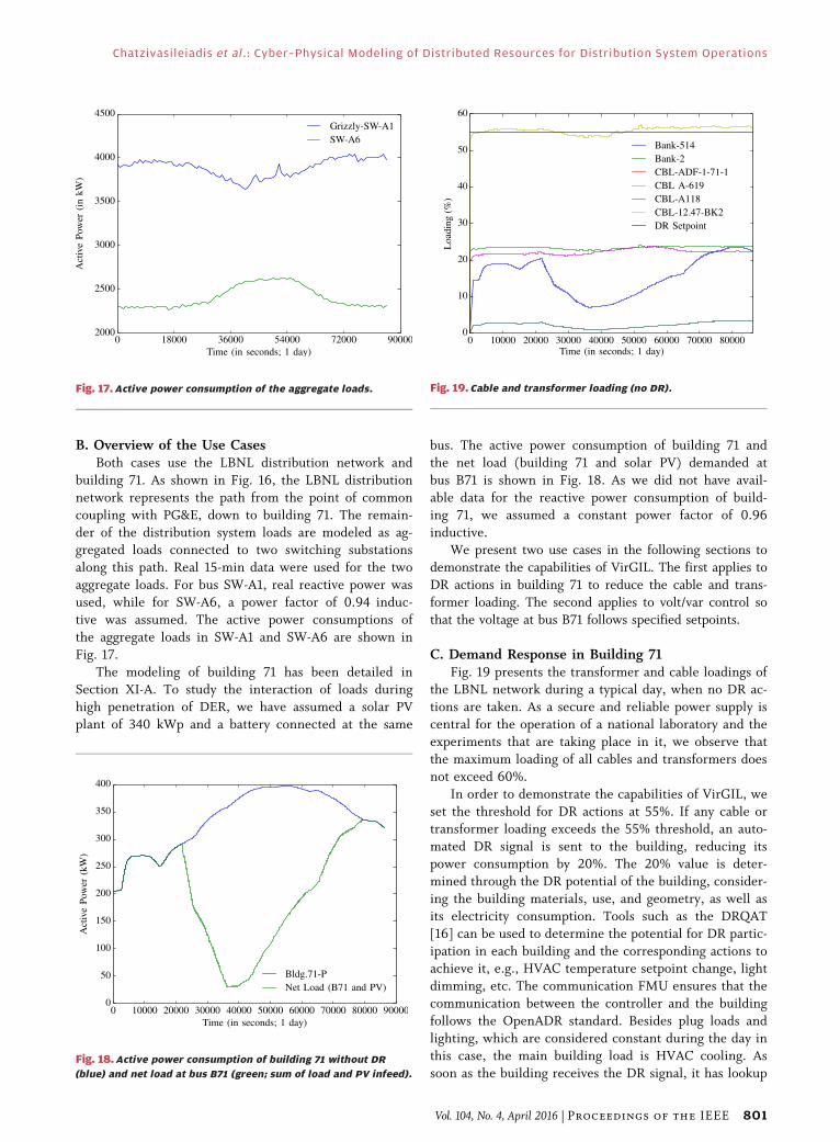
C. Demand Response in Building 71Fig. 19 presents the transformer and cable loadings of

the LBNL network during a typical day, when no DR ac-

tions are taken. As a secure and reliable power supply is

central for the operation of a national laboratory and the

experiments that are taking place in it, we observe that

the maximum loading of all cables and transformers does

not exceed 60%.

In order to demonstrate the capabilities of VirGIL, we

set the threshold for DR actions at 55%. If any cable ortransformer loading exceeds the 55% threshold, an auto-

mated DR signal is sent to the building, reducing its

power consumption by 20%. The 20% value is deter-

mined through the DR potential of the building, consider-

ing the building materials, use, and geometry, as well as

its electricity consumption. Tools such as the DRQAT

[16] can be used to determine the potential for DR partic-

ipation in each building and the corresponding actions toachieve it, e.g., HVAC temperature setpoint change, light

dimming, etc. The communication FMU ensures that the

communication between the controller and the building

follows the OpenADR standard. Besides plug loads and

lighting, which are considered constant during the day in

this case, the main building load is HVAC cooling. As

soon as the building receives the DR signal, it has lookup

Fig. 17. Active power consumption of the aggregate loads.

Fig. 18. Active power consumption of building 71 without DR

(blue) and net load at bus B71 (green; sum of load and PV infeed).

Fig. 19. Cable and transformer loading (no DR).



tables that transform the power reduction to increased

setpoints for the HVAC operation, as higher operating

temperatures reduce the necessary cooling power.

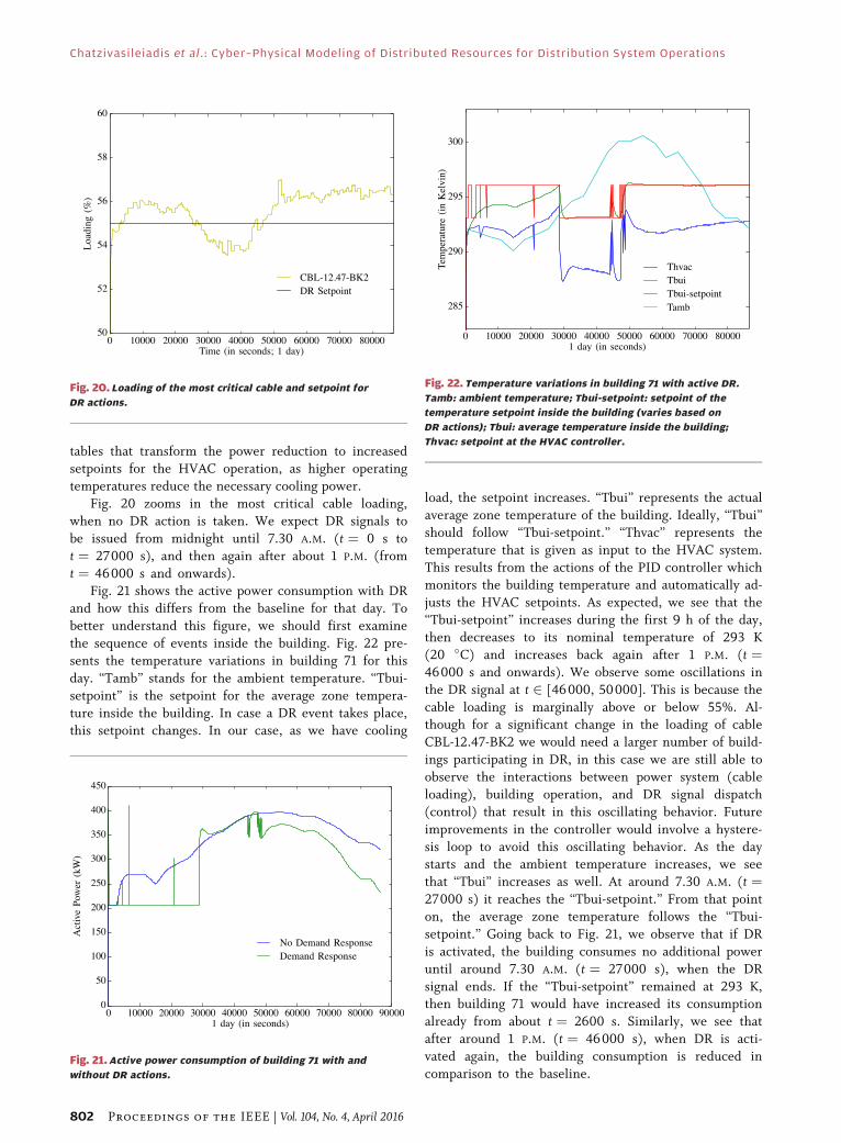
Fig. 20 zooms in the most critical cable loading,

when no DR action is taken. We expect DR signals to

be issued from midnight until 7.30 A.M. (t ¼ 0 s to

t ¼ 27000 s), and then again after about 1 P.M. (from

t ¼ 46000 s and onwards).Fig. 21 shows the active power consumption with DR

and how this differs from the baseline for that day. To

better understand this figure, we should first examine

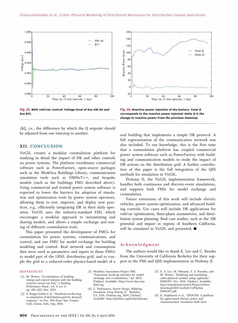
the sequence of events inside the building. Fig. 22 pre-

sents the temperature variations in building 71 for this

day. “Tamb” stands for the ambient temperature. “Tbui-

setpoint” is the setpoint for the average zone tempera-

ture inside the building. In case a DR event takes place,this setpoint changes. In our case, as we have cooling

load, the setpoint increases. “Tbui” represents the actual

average zone temperature of the building. Ideally, “Tbui”

should follow “Tbui-setpoint.” “Thvac” represents the

temperature that is given as input to the HVAC system.

This results from the actions of the PID controller whichmonitors the building temperature and automatically ad-

justs the HVAC setpoints. As expected, we see that the

“Tbui-setpoint” increases during the first 9 h of the day,

then decreases to its nominal temperature of 293 K

(20 C) and increases back again after 1 P.M. (t ¼46000 s and onwards). We observe some oscillations in

the DR signal at t 2 [46000, 50000]. This is because the

cable loading is marginally above or below 55%. Al-though for a significant change in the loading of cable

CBL-12.47-BK2 we would need a larger number of build-

ings participating in DR, in this case we are still able to

observe the interactions between power system (cable

loading), building operation, and DR signal dispatch

(control) that result in this oscillating behavior. Future

improvements in the controller would involve a hystere-

sis loop to avoid this oscillating behavior. As the daystarts and the ambient temperature increases, we see

that “Tbui” increases as well. At around 7.30 A.M. (t ¼27000 s) it reaches the “Tbui-setpoint.” From that point

on, the average zone temperature follows the “Tbui-

setpoint.” Going back to Fig. 21, we observe that if DR

is activated, the building consumes no additional power

until around 7.30 A.M. (t ¼ 27000 s), when the DR

signal ends. If the “Tbui-setpoint” remained at 293 K,then building 71 would have increased its consumption

already from about t ¼ 2600 s. Similarly, we see that

after around 1 P.M. (t ¼ 46000 s), when DR is acti-

vated again, the building consumption is reduced in

comparison to the baseline.

Fig. 20. Loading of the most critical cable and setpoint for

DR actions.

Fig. 21. Active power consumption of building 71 with and

without DR actions.

Fig. 22. Temperature variations in building 71 with active DR.

Tamb: ambient temperature; Tbui-setpoint: setpoint of the

temperature setpoint inside the building (varies based on

DR actions); Tbui: average temperature inside the building;

Thvac: setpoint at the HVAC controller.



Fig. 23 compares the active power consumption of

building 71 when there are no communication delays. In

our base case, shown in Fig. 21, the polling frequency of

the DR client in the communication FMU was set at

30 s, which means that every DR signal was sent with30 s. The actual communication delays that were also

modeled in this setup did not exceed on average 500 ms.

In Fig. 23, we do not observe major differences between

the two cases. This is probably due to the fact that the

building dynamics are slow enough to not be signifi-

cantly affected by a 30-s delay. Still, we observe that at

about t ¼ 45000 s, the oscillations of the active power

have a higher magnitude when the signal is transmittedwith no delay. This is expected due to the more direct

response to the signal.

Concluding this use case, we see how VirGIL is able

to accurately model and simulate the interactions be-

tween buildings, communication, and power systems.

We have observed how a power system event leads to a

DR signal, and how this affects the building operation.

At the same time, we were able to represent the effect ofthe communication delays, and measure the effect of the

building actions back to the power grid. In [2], we inves-

tigated further the effect of the communication infra-

structure in a hardware-in-the-loop setting.

D. Volt/Var Control at Bus B71In this use case, we demonstrate how VirGIL can be

used for volt/var control. In the LBNL network we haveinstalled three microphasor measurement units (�PMUs)

[32]. One of them is located at bus SW-A6 and one more

at bus B71. �PMUs are units that can measure with high

fidelity voltage, current, and voltage angle.

In this case, we assume that we receive as inputs the

voltage from the �PMU measurements at buses SW-A6

and B71. The goal is that the voltage at bus B71 should

follow the voltage at SW-A6, by appropriately controlling

the reactive power infeed of the battery.

The controller solves the following equation in order

to find the necessary reactive power infeed:

U12¼ U2þðR�PþX �QÞ=U2ð Þ2þðX �P�R�QÞ2=ðU2Þ2 (12)

where

U1 ¼USW�A6 (13)

U2 ¼UB71 (14)

P ¼ PB71 � PBAT � PPV (15)

Q ¼ PB71 � QBAT � QPV (16)

R ¼ RBank�514 þ RCBL�ADF�1�71�1 þ RA�619 (17)

X ¼ RBank�514 þ XCBL�ADF�1�71�1 þ XA�619: (18)

Fig. 24 presents the voltage at the two buses if no

volt/var control actions take place. We can observe how

the PV infeed, starting at about 6 A.M. until about 10 A.M.

(t ¼ 24 to t ¼ 40 quarters), increases the voltage momen-

tarily, while in general the voltage level at bus B71 is de-

creasing as the building consumption increases. Once

again, we observe that the LBNL network is sufficiently(over)dimensioned so that we do not observe significant

voltage drops at the end of the feeders. Still this use case

demonstrates VirGIL performance and characteristics.

Fig. 25 presents the same voltages, but with volt/var con-

trol, so that VB71 tracks the voltage VSW�A6 at bus SW-A6.

The required reactive power infeed from the battery is

presented in Fig. 26. In the same figure, we also present

Fig. 23. Active power consumption of building 71 with DR, with

and without signal communication delays.

Fig. 24.Without volt/var control: Voltage level of bus SW-A6 and

bus B71.



�Q, i.e., the difference by which the Q setpoint should

be adjusted from one timestep to another.

XII. CONCLUSION

VirGIL creates a modular cosimulation platform for

studying in detail the impact of DR and other controls

on power systems. The platform coordinates commercial

software such as PowerFactory, open-source packages

such as the Modelica Buildings Library, communicationsimulation tools such as OMNeT++, and bespoke

models (such as the buildings FMU described above).

Using commercial and trusted power system software is

expected to lower the barriers for adoption of simula-

tion and optimization tools by power system operators,

allowing them to test, improve, and deploy new prac-

tices, e.g., efficiently integrating DR in their daily oper-

ation. VirGIL uses the industry-standard FMI, whichencourages a modular approach to instantiating and

sharing models, and allows a simple exchange and test-

ing of different cosimulation tools.

This paper presented the development of FMUs for

cosimulation for power systems, communications, and

control, and one FMU for model exchange for building

modeling and control. Real network and consumption

data were used as parameters and inputs to these FMUsto model part of the LBNL distribution grid, and to cou-

ple the grid to a reduced-order physics-based model of a

real building that implements a simple DR protocol. A

full representation of the communication network wasalso included. To our knowledge, this is the first time

that a cosimulation platform has coupled commercial

power system software such as PowerFactory with build-

ing and communication models to study the impact of

DR actions on the distribution grid. A further contribu-

tion of this paper is the full integration of the QSS

methods for simulation in VirGIL.

Ptolemy II, the VirGIL implementation framework,handles both continuous and discrete-event simulations,

and supports both FMIs for model exchange and

cosimulation.

Future extensions of this work will include electric

vehicles, power system optimization, and advanced build-

ing controls. Use cases will include DR applications for

volt/var optimization, three-phase asymmetries, and distri-

bution system planning. Real case studies, such as the DRpotential and impact in regions of Southern California,

will be simulated in VirGIL and presented. h

Acknowledgment

The authors would like to thank E. Lee and C. Brooks

from the University of California Berkeley for their sup-

port in the FMI and QSS implementation in Ptolemy II.

REFERENCES

[1] M. Wetter, “Co-simulation of buildingenergy and control systems with the buildingcontrols virtual test bed,” J. BuildingPerformance Simul., vol. 4, no. 3,pp. 185–203, Nov. 2011.

[2] S. Rotger-Griful et al., “Hardware-in-the-loopco-simulation of distribution grid for demandresponse,” in Proc. 19th Power Syst. Comput.Conf., Genoa, Italy, Aug. 2016.

[3] Modelica Association Project FMI,“Functional mock-up interface for modelexchange and co-simulation,” Jul. 2014.[Online]. Available: https://www.fmi-stan-dard.org

[4] C. Ptolemaeus, System Design, Modeling,Simulation Using Ptolemy II. Berkeley,CA, USA: Ptolemy.org, 2014. [Online].Available: http://ptolemy.org/books/Systems

[5] E. A. Lee, M. Niknami, T. S. Nouidui, andM. Wetter, “Modeling and simulatingcyber-physical systems using cyphysim,”EMSOFT, Oct. 2015. [Online]. Available:http://simulationresearch.lbl.gov/wetter/download/2015-LeeEtAl CyPhySimEMSOFT.pdf.

[6] K. Hopkinson et al., “EPOCHS: A platformfor agent-based electric power andcommunication simulation built from

Fig. 25.With volt/var control: Voltage level of bus SW-A6 and

bus B71.

Fig. 26. Reactive power injection of the battery. Total Q

corresponds to the reactive power injected. Delta Q is the

change in reactive power from the previous timestep.



commercial off-the-shelf components,”IEEE Trans. Power Syst., vol. 21, no. 2,pp. 548–558, May 2006.

[7] H. Lin, S. Sambamoorthy, S. Shukla, J. Thorp,and L. Mili, “Power system andcommunication network co-simulation forsmart grid applications,” in Proc. IEEEPES Innovative Smart Grid Technol.,DOI: 10.1109/ISGT.2011.5759166.

[8] M. Levesque, D. Q. Xu, G. Joos, andM. Maier, “Communications and powerdistribution network co-simulation formultidisciplinary smart gridexperimentations,” in Proc. 45th Annu.Simul. Symp., San Diego, CA, USA, 2012,pp. 2:1–2:7.

[9] R. Bottura et al., “SITL and HLAco-simulation platforms: Tools for analysisof the integrated ICT and electric powersystem,” in Proc. IEEE EUROCON,pp. 918–925.

[10] M. Stifter et al., “Co-simulation of compo-nents, controls and power systems based onopen source software,” in Proc. IEEE PowerEnergy Soc. Gen. Meeting, DOI: 10.1109/PESMG.2013.6672388.

[11] P. Palensky, E. Widl, and A. Elsheikh,“Simulating cyber-physical energy systems:Challenges, tools and methods,” IEEE Trans.Syst. Man Cybern., Syst., vol. 44, no. 3,pp. 318–326, Mar. 2014.

[12] D. Chassin, K. Schneider, andC. Gerkensmeyer, “GridLAB-D: Anopen-source power systems modeling andsimulation environment,” in Proc. IEEEPES Transm. Distrib. Conf. Expo.,DOI: 10.1109/TDC.2008.4517260.

[13] S. Muller, H. Georg, C. Rehtanz, andC. Wietfeld, “Hybrid simulation of powersystems and ICT for real-time applications,”in Proc. 3rd IEEE PES Int. Conf. Exhibit.

Innovative Smart Grid Technol.,DOI: 10.1109/ISGTEurope.2012.6465734.

[14] T. Nouidui, M. Wetter, and W. Zuo,“Functional mock-up unit for co-simulationimport in energyplus,” J. BuildingPerformance Simul., vol. 7, no. 3,pp. 192–202, 2014.

[15] D. Sturzenegger, D. Gyalistras,V. Semeraro, M. Morari, and R. Smith,“BRCM matlab toolbox: Model generationfor model predictive building control,”in Proc. Amer. Control Conf.,DOI: 10.1109/ACC.2014.6858967.

[16] R. Yin, P. Xu, M. A. Piette, and S. Kiliccote,“Study on auto-DR and pre-cooling ofcommercial buildings with thermal mass inCalifornia,” Energy Buildings, vol. 42, no. 7,pp. 967–975, Jul. 2010.

[17] Commercial Prototype Building Models.[Online]. Available: http://www.energy-codes.gov/commercial-prototype-building-models

[18] K. Glover, “All optimal hankel-normapproximations of linear multi-variablesystems and their L-inf error bounds,” Int. J.Control, vol. 39, no. 6, pp. 1115–1193, 1984.

[19] K. Zhou, “Frequency-weighted modelreduction with L error bounds,” Syst. ControlLett., vol. 21, no. 2, pp. 115–125, 1993.

[20] M. Wetter, W. Zuo, T. S. Nouidui, andX. Pang, “Modelica buildings library,”J. Building Performance Simul., vol. 7, no. 4,pp. 253–270, 2014.

[21] OMNeT++. [Online]. Available: https://www.omnetpp.org/

[22] T. Godfrey et al., “Modeling smart grid ap-plications with co-simulation,” in Proc. 1stIEEE Int. Conf. Smart Grid Commun., 2010,pp. 291–296.

[23] C. Muller, H. Georg, and C. Wietfeld,“A modularized and distributed simulation

environment for scalability analysis of smartgrid ICT infrastructures,” in Proc. 5th Int.Conf. Simul. Tools Tech., 2012, pp. 327–330.

[24] K. Mets, J. A. Ojea, and C. Develder,“Combining power and communicationnetwork simulation for cost-effective smartgrid analysis,” IEEE Commun. Surv. Tut.,vol. 16, no. 3, pp. 1771–1796, 2014.

[25] M. Bredel and M. Bergner, “On the accuracyof IEEE 802. 11 g wireless LAN simulationsusing OMNeT++,” in Proc. 2nd Int. Conf.Simul. Tools Tech., 2011, Art. no. 81.

[26] A. Virdis, G. Stea, and G. Nardini,“SimuLTE—A modular system-levelsimulator for LTE//LTE—A networks basedon OMNeT þþ,” in Proc. SimulTech, 2014,pp. 28–30.

[27] E. Weing, H. Lehn, and K. Wehrle,“A performance comparison of recentnetwork simulators,” in Proc. IEEE Int.Conf. Commun., 2009, DOI: 10.1109/ICC.2009.5198657.

[28] Openadr Alliance. [Online]. Available:http://www.openadr.org/

[29] Demand Response Research Center,“Openadr.” [Online]. Available:http://drrc.lbl.gov/openadr

[30] F. E. Cellier and E. Kofman, ContinuousSystem Simulation. New York, NY, USA:Springer-Verlag, 2006.

[31] G. Migoni, M. Bortolotto, E. Kofman, andF. E. Cellier, “Linearly implicitquantization-based integration methodsfor stiff ordinary differential equations,”Simul. Model. Practice Theory, vol. 35,pp. 118–136, 2013.

[32] E. Stewart et al., “Addressing the challengesfor integrating micro-synchrophasor datawith operational system applications,” inProc. PES Gen. Meeting Conf. Expo.,DOI: 10.1109/PESGM.2014.6938994.

ABOUT THE AUTHORS

Spyros Chatzivasileiadis (Member, IEEE) re-

ceived the Diploma in electrical and computer

engineering from the National Technical Univer-

sity of Athens (NTUA), Athens, Greece, in 2007

and the Ph.D. from ETH Zurich, Switzerland, in

2013, with focus on the integration of HVDC lines

in power system planning and operation.

He is a Postdoctoral Researcher at the

Massachusetts Institute of Technology (MIT),

Cambridge, MA, USA. Until July 2015, he was with

Lawrence Berkeley National Laboratory (LBNL), Berkeley, CA, USA,

where he worked on dc microgrids and cosimulation tools to integrate

demand response in power systems. His research interests are on

power system optimization and control.

Marco Bonvini received the M.S. degree in com-

puter science and the Ph.D. degree in systems

and controls from the Politecnico di Milano,

Milan, Italy, in 2009 and 2013, respectively.

Later he worked at Lawrence Berkeley Na-

tional Laboratory (LBNL), Berkeley, CA, USA,

where he developed building simulation models

and integrated them with optimization and fault

detection algorithms to improve the operation of

buildings. Currently, he is a Data Scientist at

Whiskerlabs, Oakland, CA, USA, where he focuses on nonintrusive load

monitoring.

Javier Matanza received an electrical engineer-

ing degree from the Polytechnic University of

Valencia, Valencia, Spain, in 2008 and the Ph.D.

degree from the Comillas Pontifical University,

Madrid, Spain, in 2013.

He is a Research Professional at the Institute

for Research in Technology (IIT) and an Assistant

Professor at the Comillas Pontifical University.

His current interests are in powerline communi-

cation technologies and in communication net-

work simulations.

Rongxin Yin received the M.Sc. degree in me-

chanical engineering from Tongji University,

China, in 2009 and the M.Sc. degree in building

science from University of California at Berkeley,

CA, USA, in 2013.

He is a Senior Scientific Engineering Associate

in the Grid Integration Group, Lawrence Berkeley

National Laboratory (LBNL), Berkeley, CA, USA.

He has been at LBNL since 2007 and focuses his

career on building science, energy and buildings,

and demand to grid. His research focuses on energy efficiency and de-

mand response (EE&DR) in commercial buildings.



Thierry S. Nouidui received the M.S. degree in

electrical engineering from the University of Kiel,

Kiel, Germany, in 2004 and the Ph.D. degree in

building physics from the University of Stuttgart,

Stuttgart, Germany, in 2008.

He is a Principal Scientific Engineering Associ-

ate in the Simulation Research Group, Lawrence

Berkeley National Laboratory (LBNL), Berkeley,

CA, USA. His current research is focused on de-

veloping and deploying new generation of build-

ing performance computational tools for the design and operation of

buildings and communities.

Emre C. Kara (Member, IEEE) received the M.Sc.

degree in building engineering from Delft Uni-

versity of Technology, Delft, The Netherlands,

in 2010 and the Ph.D. degree in civil and envi-

ronmental engineering from Carnegie Mellon

University, Pittsburgh, PA, USA, in 2014.

He is currently a Postdoctoral Researcher at

Lawrence Berkeley National Laboratory (LBNL),

Berkeley, CA, USA. His research interests include

understanding the energy use of buildings,

modeling, and control of building loads to provide demand response

services to increase power system reliability.

Rajiv Parmar received the B.Sc. degree in com-

puter engineering and the M.Eng. degree in elec-

trical engineering specializing in energy and

environment from the University of Calgary,

Calgary, AB, Canada, in 2004 and 2011, respectively.

Until June 2015 he was a Software Developer at

Lawrence Berkeley National Laboratory (LBNL),

Berkeley, CA, USA. He has several years of experi-

ence in the software industry in Canada and the

United States, in areas such as energy, demand re-

sponse, SCADA systems, communications, quality, and security.

David Lorenzetti received the B.S. degree in

electrical and comuputer engineering, from the

University of Cincinnati, in 1986, and the M.S.

and Ph.D. degrees in building technology, from

Massachusetts Institute of Technology, in 1992

and 1997 respectively.

Currently he is with Lawrence Berkeley Na-

tional Laboratory (LBNL), Berkeley, CA, USA. His

research interests include whole-building airflow,

pollutant transport, and energy; and applying nu-

merical simulation to study problems of life safety and energy conser-

vation in buildings.

Michael Wetter received the B.S. degree in en-

ergy and building technologies from the Univer-

sity of Applied Sciences at Luzern, Switzerland,

in 1995, and the Ph.D. degree in mechanical en-

gineering from the University of California,

Berkeley, CA, USA, in 2004.

He is a Computational Staff Scientist and the

Deputy Leader of the Simulation Research Group

at Lawrence Berkeley National Laboratory

(LBNL), Berkeley, CA, USA. His research includes

integrating building performance simulation tools into the research

process, as well as their use for design and operation of buildings. At

LBNL, he is developing the Modelica Buildings library for building en-

ergy and control systems, a prototype implementation of a new com-

puting engine for EnergyPlus, cosimulation tools based on the

functional mockup interface standard, the building controls virtual

testbed software for cosimulation and model-based operation and

CyPhySim, a cyber–physical system simulator based on Ptolemy II. As

the cooperating agent of the IEA EBC Annex 60, he leads a research

team from 16 countries and 40 institutes in the development of new

generation computational tools for buildings and community energy

systems between 2012 and 2017.

Dr. Wetter is the youngest Fellow of the International Building Per-

formance Simulation Association (IBPSA), a recipient of the biannual

Outstanding Young Contributor Award of IBPSA, the Treasurer of IBPSA,

and a Board Member of the Modelica North America Users Group; was

President of the U.S. Affiliate of IBPSA; and is a Member of ASHRAE and

of the Modelica Association.

Sila Kiliccote (Member, IEEE) received an Elec-

trical Engineering degree from the University of

New Hampshire, Durham, NH, USA, in 1994, and

the M.S. degree in building science from Carnegie

Mellon University, Pittsburgh, PA, USA, in 1995.

She is the Smart Grid leader at SLAC National

Accelerator Laboratory, Menlo Park, CA, USA,

and holds a part-time position as a demand re-

sponse expert at Google. Prior to joining SLAC,

she spent over ten years at Lawrence Berkeley

National Laboratory (LBNL), Berkeley, CA, USA, as a Deputy of the De-

mand Response Research Center and leading the grid integration initia-

tives, where she worked with teams to develop OpenADR, Virtual Grid

Integration Laboratory (VirGIL), and explored the use of models with

data from micro-PMUs for distribution systems.



INVITED PAPER Cyber–PhysicalModelingof ...

Documents

Transcript of INVITED PAPER Cyber–PhysicalModelingof ...